~ .

Interim Analyses in Clinical Trials: Classical vs.· ad hoc vs. Bayesian Approaches

Donald A. Berry*

University of Minnesota School of Statistics

Technical Report No. 418 May 1983

*Research supported in part by NSF grant NSF/MCS 8102477

ABSTRACT

Interim analysis in clinical trials is discussed from the point of

view of both classical hypothesis testing and Bayesian inference. The

application of P-values in this setting is criticized. The ad hoc approach

is recommended over adjusting P-values for the possibility of stopping the

trial earlier or later. A Bayesian approach is presented in which stopping

occurs when the probability that one treatment is better exceeds a specified

value.

Key words and phrases: Clinical trials, interim analysis, P-values,

hypothesis testing, Bayesian inference, posterior probability,

likelihood principle.

'

1. Introduction

When a researcher peruses accumulating data from a clinical trial

with a possibility of early termination, certain kinds of inferences to

be drawn from the trial may be affected. This is well understood by

biometricians but not by researchers (McPherson 1982). Readers of

medical journals do not ask whether a trial might have been stopped

sooner· but was not; they take the data at face value. And yet classical

Neyman-Pearsonian tests require specifying all possibilities in advance.

Important deviations from protocol can make classical inferences impossi­

ble. This is one reason, perhaps the most important reason, that sequen­

tial designs of clinical trials have been so little used (Simon 1977,

Byar et al. 1974).

Biostatisticians have had a substantial impact on this aspect of the

design of clinical trials. Dissidents (Anscombe 1963, Cornfield 1966,

Weinstein 1974, Berry 1980) have had essentially no effect on statistical

practice. This controversial issue is an important one: at stake is

human suffering and financial resources of sponsoring agencies and

pharmaceutical companies. If some trials last too long and others end

prematurely because statisticians disallow looking at accumulating data

or continuing beyond the planned trial termination, then the statistical

principle on which this is based should have a solid foundation.

A purpose of this paper is to describe implications of classical

hypothesis testing for interim analysis. Strict adherence to classical

testing is criticized. A less rigid view--one that will offend some

-1-

7

purists but appeal to clinicians--is advocated. The Bayesian approach

is discussed.

At the heart of the controversy is the distinction between P-values

and probabilities of hypotheses. This issue is discussed in the next two

sections; a likelihood approach is discussed in Section 3. The classical

approach to interim analysis is discussed in Sections 4 and 5 and compared

to a Bayesian approach in Section 5. These are related in Section 6 to

an ad hoc approach taken by most researchers. This ad hoc approach uses

classical fixed size analyses imbedded in a Bayesian philosophy.

2. P-values and Neyman-Pearson Testing

Most consumers of statistical inference incorrectly regard a P-value

as related to the probability of the truth of a null hypothesis. They

act as though H0

is false when the P-value is sufficiently small--usually

less than 0.05--feeling that their action is correct with some high

probability.

Calculating the probability of H0

from available data requires the

use of Bayes's theorem. This in turn requires a probability assessment

of H0

separate from (or prior to) the data, and pushes many 11 Bayesians"

to adopt a subjective view of probability (Savage 1954). Such blatant

subjectivism repels many statisticians. They refuse to pay this price

and so reject all Bayesian thought.

P-values are understood by trained statisticians but by few others.

For example, two M.D.'s (Diamond and Forrester 1983) asked 24 of their

colleagues this multiple choice question: "What would you conclude if a

properly conducted, randomized clinical trial of a treatment was reported

-2-

7

to have resulted in a beneficial response (p < 0.05)?

1. Having obtained the observed response, the chances are less than

5% that the therapy is not effective.

2. The chances are less than 5% of not having obtained the observed

response if the therapy is effective.

3. The chances are less than 5% of having obtained the observed

response if the therapy is not effective.

4. None of the above. 11

The authors say that all responders had difficulty distinguishing the

subtle differences between the choices. Of the 24 responders, 11 chose #1

and one other gave an 11 incorrect 11 answer. The authors say #3 is correct.

However, #3 requires the insertion "or more extreme responses 11 to be correct.

As the choices stand, #4 is correct! Interestingly, 19 of the 24 said they

would prefer to know the answer to #1, the (Bayesian) posterior probability;

in second place was #2.

Diamond and Forrester (1983) cite a number of important large-scale

clinical trials in which a high degree of significance was obtained origi­

nally, but the conclusion was later contradicted. Blaming P-values, they

make what they call an 11arrogant pronouncement:" "The published conclusions

of many clinical trials are ill-founded, and may be wrong." They go on

to claim that these mistakes would not have been made using a Bayesian

approach ..

Clinical trials whose results are eventually contradicted do little

for the credibility of statistics and statisticians. Regardless of what

P-values really mean, consumers will expect that conclusions from clinical

-3-

trials (reject H0

, e.g.) are correct with some high probability. This

expectation involves posterior probabilities and not P-values. If some­

one were to find that more than half the conclusions (at P<0.05) of all

published clinical trials were wrong, this would not be inconsistent with

the inferences made from the results of the trials! Disheartening but not

inconsistent.

3. Likelihoods vs. Classical Tests

P-values are tail areas. They are calculated by integrating over

results more extreme than that obtained, but these more extreme results

have not themselves been observed. This characteristic prompted Harold

Jeffreys's (1961) criticism: II a hypothesis which may be true may be

rejected because it has not predicted observable results which have not

occurred." The size of the tail affects the inference.

As an example, consider the following problem: Ten tosses of a

coin result in 2 heads and 8 tails; test the hypothesis that the coin

is fair against the one-sided alternative that the probability of heads

is less than 1/2. The solution depends critically on the intentions of

the tosser, but when confronted with this problem, few people, statisti­

cians included, ask the key question: Why did the tosser choose to stop?

If you think this question is irrelevant then you do not take hypothesis

testing as seriously as do many statisticians--and you might be a Bayesian

at heart!

Solution 1. Suppose the tosser planned ten tosses and would have

allowed nothing to stand in the way of this objective. Then the appropriate

-4-

;

distribution is binomial:

p = [(l~)+ (ln + c~)J m 10,; 0.055.

Solution 2. Suppose the tosser planned to obtain two heads and

would have tossed as long as necessary. Then the appropriate distribution

is negative binomial:

10 11 12 p = 9(1) + 10(½) + 11(½) + .•. ~ 0.020.

Solution 3. Suppose the tosser planned to stop and reject the null

hypothesis if there were O heads in the first 4 tosses, 1 head after 7 tosses,

or 2 after 10--stopping after 10 tosses in any case. Backward induction

gives

P = 41/512 ~ 0.080

Solution 4 .. Suppose the tosser planned to continue indefinitely,

stopping to reject H0

as in Solution 3, but also if there were 3 heads in

14 tosses, 4 in 17, etc. An iterative procedure gives

P ~ 0. 145.

Solution 5. Suppose the tosser planned to stop when dinner was ready

and reject H0

i"f the proportion of heads was no greater than 0.2. No

P-value can be calculated and such data cannot be analyzed legitimately

using the Neyman-Pearson approach.

The possibility of different solutions depending on the intentions

of the experimenter are counter to the likelihood principle (Cornfield

-5-

1966, Barnett 1973). This principle says, roughly speaking, that two

sets of data which give rise to the same likelihood function should give

rise to the same inferences. In the above problem the likelihood of p,

the probability of heads, is proportional to

in all five solutions; the proportionality constant which makes this a

probability for the random variable in question varies depending on the

solution but is immaterial in the likelihood.

The likelihood principle implies that the question "Why did the

tosser stop?" is not relevant for making inferences. (This assumes, of

course, that the decision to stop is not a function of p, or of future

observations--for example, tossing stopped when the coin was lost and

it is more likely to be lost when it is about to land heads.)

The likelihood principle requires a model under which the data are

assumed to be produced. If the model is wrong (and it frequently is!)

then the inferences can be wrong for that reason. A weaker version which

does not rely on a particular likelihood is the following, which is

related to the Conditionality Principle (Berger 1980).

Data Principle: Inferences depend only on the data obtained and

the experiment performed, and not on data not obtained or on experiments

contemplated but not performed.

Objecting to using error probabilities in experimentation, Anscombe

(1963) says: "'sequential analysis' is a hoax. The correct statistical

-6-

analysis of the observations consists primarily of quoting the likelihood

function. So long as all observations made are fairly reported, the

sequential stopping rule that may or may not have been followed is irrele­

vant. The experimenter should feel entirely uninhibited about continuing

or discontinuing his trial, changing his mind about the stopping rule in

the middle, etc., because the interpretation of the observations will be

based on what was observed, and not on what might have been observed but

wasn't. 11

Since tail areas are not consistent with the likelihood principle,

"likelihooders" require another mode of inference. One such is the like­

lihood ratio test for simple n~ll and simple alternative hypotheses (but

not the generalization for compound hypotheses which uses the maximum

of the likelihood function in the ratio). Another is the Bayes test,

which applies for arbitrary hypotheses. An example is described below.

Data from an actual trial (in which the likelihood p2(1-p)8 con­

sidered above arises at one point) were considered by Cutler, et al.

(1966) and Lachin in(Tygstrup, et al. 1982, pp. 241-242). This sequential

trial (Freireich 1963) involved two treatments for acute leukemia.

Patients were treated in matched pairs and the outcome of interest was

time to remission; only the better treatment in each pair was analyzed.

The data are shown in Table 1. Using repeated significance testing analy­

sis, P < 0.05 was attained with the 18th pair, at which time the remaining

three pairs had already been randomized to treatment. (An interesting

dilemna presents itself for the classical purist: to what extent should

the last three pairs affect the P-value in this approach?--presumably not

-7-

at all. But I prefer an approach to inference that allows for different

inferences when the last three favor A and when they favor B.)

The results of various analyses are also shown in Table 1. These are

described below.

Let pB = 1-pA be the probability that treatment Bis preferred.

Assume that information regarding effectiveness of the two treatments

apart from the trial is symmetric. Consider testing H0

: PA= r vs.

H1: pB = r (that is, PA= 1 - r) for fixed r. Also require that error

probabilities a and B be equal. Wald's sequential likelihood ratio test

(SLRT) (Lindgren 1976, pp. 310-317) is to continue as long as

-1 C <A< c,

_, where c = a - land A is the likelihood ratio:

n n n -n = r A(l-r) B = (__r.__) A B.

A n n 1-r ' r B(l-r) A

nA and n8 are the numbers of preferences for A and B respectively. In

general, nA and n8 are jointly sufficient; nA - nB is sufficient here

because H0 and H1 are simple and symmetric. The appropriate P-value is

(l+A)-l.

P-values for the SLRT with r = 0.55, 0.6, 0.7, and 0.8 are shown for

the accumulating data in Table 1. Significance is reached after 21, 12,

8, and 7 pairs, respectively.

These P-values are also Bayesian probabilities in the following set-up.

Suppose the prior probabilities of pA =rand p8 =rare both 0.5. Then,

-8-

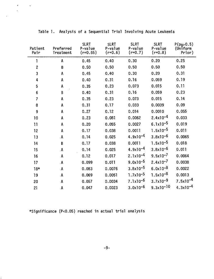
Table l. Analysis of a Sequential Trial Involving Acute Leukemia

SLRT SLRT SLRT SLRT P(Ps>O. 5) Patient Preferred P-value P-value P-value P-value (Uniform Pair Treatment (r=0.55) (r=0.6) (r=0.7) (r=0.8) Prior)

l A 0.45 0.40 0.30 0.20 0.25

2 B 0.50 0.50 0.50 0.50 0.50

3 A 0.45 0.40 0.30 0.20 0.31

4 A 0.40 0.31 0.16 0.059 0.19

5 A 0.35 0.23 0.073 0.015 0.11

6 8 0.40 0. 31 0.16 0.059 0.23

7 A 0.35 0.23 0.073 0.015 0.14

8 A 0.31 0.17 0.033 0.0039 0.09

9 A 0.27 0.12 0.014 0. 0010 0.055

10 A 0.23 0.081 0.0062 2.4x10-4 0.033

11 A 0.20 0.055 0.0027 6. l xl o-5 0.019

12 A 0. 17 0.038 0.0011 1. 5xl o-5 0.011

13 A 0.14 0.025 4.9xlo-4 3.8xlo-6 0.0065

14 8 0.17 0.038 0. 0011 l.5x10-s 0.018

15 A 0.14 0.025 4.9xlo-4 3.8x10-6 0. 011

16 A 0.12 0.017 2. 1 xl o-4 9.5x10-7 0.0064

17 A 0.099 0.011 9.0xlo-5 2.4x10-7 0.0038

18* A 0.083 0.0076 3.8xlo-5 6.0xlo-8 0.0022

19 A 0.069 0.0051 1.1x10-5 l.Sxl o-8 0. 0013

20 A 0.057 0.0034 1.1x10-6 3.7xlo-9 7.5xlo-4

21 A 0.047 0.0023 3.oxio-6 9.3xlo-10 4.3x10-4

*Significance (P<0.05) reached in actual trial analysis

-9-

by Bayes's theorem, the current probability of p8 = r is

n n (0.5)r 8(1-r) A

n n n n (0.S)r 8(1-r) A+(0.5)r A(l-r) B

which is the P-value indicated above.

= 1 l+A'

The last column in Table 1 is the probability that treatment Bis

better than treatment A (that is, p8 > 0.5) given the current data when

the prior distribution for p8 (and therefore also pA) is the uniform

density on the interval (0,1). From Bayes's theorem,

an incomplete beta function. (This probability is not a function of

nA-nB alone.) This becomes less than 0.05 with the tenth pair and

approximately 0.01 with the twelfth. The uniform prior may not be

unrealistic in view of the following claim by Lachin (Tygstrup 1982,

pp. 241-242): "When a group of physicians are shown these results line

by line and asked when they would have been ethically compelled to stop

the study, u sua 11 y few wou 1 d be wi 11 i ng to go beyond the twe 1 f th pair. 11

4. Interim Analysis; An Example

A trial is planned to compare two treatments; n = 100 paired observa­

tions are involved. One interim analysis is planned halfway through the

study. If a significant mean difference is detected after 50 pairs then

the trial will be stopped and significance proclaimed. Assume the

treatment difference is normal with, for convenience, known variance.

-10-

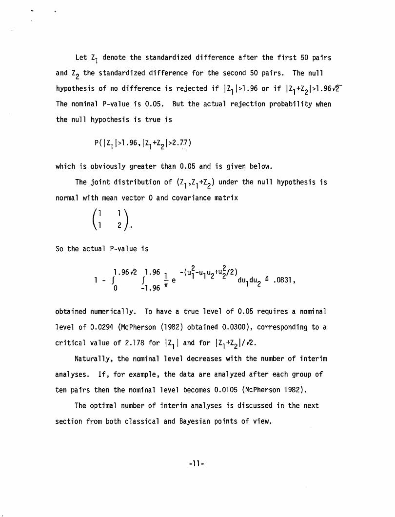
Let 21 denote the standardized difference after the first 50 pairs

and 22 the standardized difference for the second 50 pairs. The null

hypothesis of no difference is rejected if 121 l>l .96 or if l21+22l>l.96ff

The nominal P-value is 0.05. But the actual rejection probability when

the null hypothesis is true is

P ( I 2, I> 1 . 96, I Z1 +22 I >2. 7?-)

which is obviously greater than 0.05 and is given below.

The joint distribution of (Z1,z1+z2) under the null hypothesis is

normal with mean vector 0 and covariance matrix

C ~). So the actual P-value is

obtained numerically. To have a true level of 0.05 requires a nominal

level of 0.0294 (McPherson (1982) obtained 0.0300), corresponding to a

critical value of 2.178 for 121 I and for 121+22 l/t2.

Naturally, the nominal level decreases with the number of interim

analyses. If, for example, the data are analyzed after each group of

ten pairs then the nominal level becomes 0.0105 (McPherson 1982).

The optimal number of interim analyses is discussed in the next

section from both classical and Bayesian points of view.

-11-

5. The Number of Looks: Classical vs. Bayesian

The benefit of a sequential or "group sequential" approach is the

possibility that a small amount of data will be conclusive and allow for

early termination of the trial. This is an important consideration when

observations are dear. Ethical considerations when human lives are

involved have been discussed extensively (Chalmers 1982, Weinstein 1974,

Winfrey 1978). As another kind of example, consider a Phase I drug com­

parison trial in which myocardial infarctions are artificially induced in

dogs, after which extensive experimental procedures are followed and

measurements made. Such a trial can easily cost more than $1000 per dog.

Minimizing expected costs in such a trial (subject to obtaining

conclusive evidence) is equivalent to minimizing average sample size

(ASN). But adjusting P-values can make the ASN increase as the number of

looks increase, with the minimum ASN occurring in the fixed sample size

case.

For example, McPherson (1982) considers normal sampling (as in Section

4) for testing the unknown mean o = 0. The ASN depends on o as well as

the number of looks. To obtain a single measure of sample size McPherson

averages the ASN with respect to a prior distribution on o (thereby com­

bining an otherwise classical approach with a Bayesian notion). For four

different prior distributions, maximal reductions in ASN over fixed sample

sizes vary from Oto about 30% with greatest savings occurring when both

large and small deviations from o = 0 are likely a priori. In these

examples the optimal number of looks varies from 1 to 8, with ASN increasing

for numbers of looks greater than the optimum.

-12-

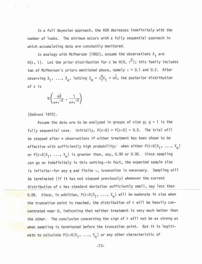
In a full Bayesian approach, the ASN decreases indefinitel y with the

number of looks . The minimum occurs with a fully sequential approach in

which accumulating data are constantly monitored.

In analogy with McPherson (1982), assume the observations Xi are

N(o, l ). Let the prior distribution for o be N(0, T2); this family includes

two of McPherson's pri ors mentioned above, namely T = 0.1 and 0.2. After

observing x1

, ... , Xn' letting Sn= r~Xi = nX, the posterior distribution

of o i s

( - ) N nX l

2 ' 2 n+T n+T

(DeGroot 1970) .

Assume the data are to be ana lyzed in groups of s ize g; g = l is the

fully sequential case. Initially, P( o>0) = P(o<0) = 0.5. The trial will

be stopped after n observations if either treatment has been shown to be

effective with sufficiently high probability: when either P( o>0jX1, ... , Xn)

or P(o<0IX1, .. . , Xn) is greater than, say, 0.90 or 0.95. Since sampling

can go on indefinitely in this setti ng- -in fact, the expected sample size

is infinite--for any g and finite T, truncation is necessary. Sampling will

be terminated (if it has not stopped previously) whenever the current

distribution of o has standard deviation sufficiently small, say less than

0.05. Since, in addition, P(&>0!X1, ... , Xn) will be moderate in size when

the truncation point i s reached, the distribution of o will be heavily con­

centrated near 0, indicating that neither treatment is very much better than

the other. The conc lusion concerning the sign of o will not be as strong as

when sampling is terminated before the truncation point. But it is legiti­

mate to calculate P( o>0jX1, ... , Xn) or any other characteristic of

-13-

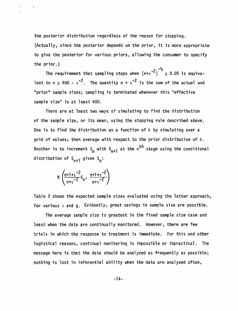
the posterior distribution regardless of the reason for stopping.

(Actually, since the posterior depends on the prior, it is more appropriate

to give the posterior for various priors, allowing the consumer to specify

the prior.) -~

The requirement that sampling stops when (n+T-2) 2

s 0.05 is equiva-

lent ton~ 400 - T-2. The quantity n + T-2 is the sum of the actual and

11 prior 11 sample sizes; sampling is terminated whenever this "effective

sample size" is at least 400.

There are at least two ways of simulating to find the distribution

of the sample size, or its mean, using the stopping rule described above.

One is to find the distribution as a function of o by simulating over a

grid of values; then average with respect to the prior distribution of o.

Another is to increment Sn with Xn+l at the nth stage using the conditional

distribution of Sn+l given Sn:

N n+l+T 5 , n+l+T ~ -2 -2) n+T-2 n n+T-2

Table 2 shows the expected sample sizes evaluated using the latter approach,

for various T and g. Evidently, great savings in sample size are possible.

The average sample size is greatest in the fixed sample size case and

least when the data are continually monitored. However, there are few

trials in which the response to treatment is immediate. For this and other

logistical reasons, continual monitoring is impossible or impractical. The

message here is that the data should be analyzed as frequently as possible;

nothing is lost in inferential ability when the data are analyzed often,

-14-

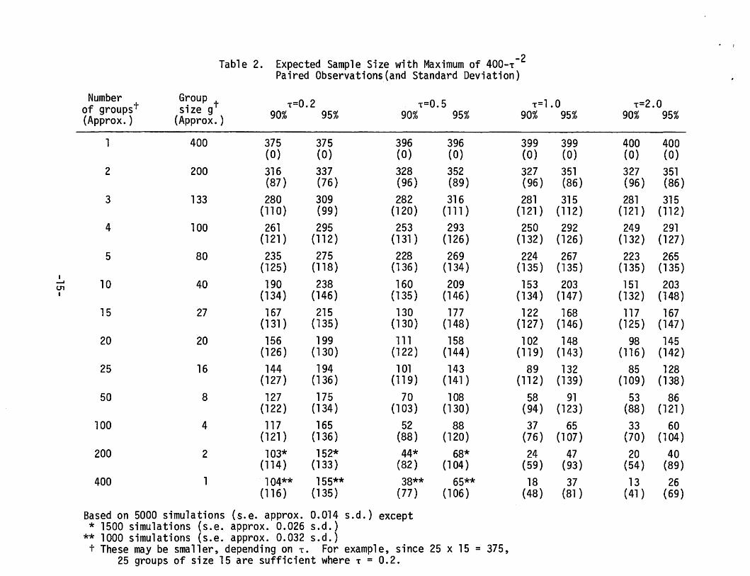
Table 2. Expected Sample Size with Maximum of 400-T -2 Paired Observations_(and Standard Deviation)

Number G~oup t T=0.2 T=0.5 T=l.O T=2.0 of groupst SlZe g 90% 95% 90% 95% 90% 95% 90% 95% {Approx.) (Approx.)

1 400 375 375 396 396 399 399 400 400 (0) (0) (0) (0) (0) (0) (0) (0)

2 200 316 337 328 352 327 351 327 351 (87) (76) {96) (89) (96) (86) (96) (86)

3 133 280 309 282 316 281 315 281 315 (110) (99) (120) (111) (121) ( 112) (121) (112)

4 100 261 295 253 293 250 292 249 291 (121) (112) (131 ) (126) (132) (126) (132) (127)

5 80 235 275 228 269 224 267 223 265 (125) (118) (136) (134) (135) ( 135) ( 135) (135)

I ..... 10 40 190 238 160 209 153 203 151 203 CJ1 I (134) (146) (135) (146) (134) (147) (132) (148)

15 27 167 215 130 177 122 168 117 167 (131) (135) (130) (148) (127) (146) (125) (147)

20 20 156 199 111 158 102 148 98 145 (126) ( 130) (122) (144) (119) (143) (116) (142)

25 16 144 194 101 143 89 132 85 128 (127) (136) (119) (141 ) (112) (139) (109) (138)

50 8 127 175 70 108 58 91 53 86 (122) (134) (103) (130) (94) (123) (88) (121)

100 4 117 165 52 88 37 65 33 60 (121) (136) {88) (120) (76} (107) (70) (104)

200 2 103* 152* 44* 68* 24 47 20 40 (114) (133) (82) (104) (59) (93) (54) (89)

400 1 104** 155** 38** 65** 18 37 13 26 ( 116) (135) (77) (106) (48) (81) ( 41) (69)

Based on 5000 simulations (s.e. approx. 0.014 s.d.) except * 1500 simulations (s.e. approx. 0.026 s.d.)

** 1000 simulations (s.e. approx. 0.032 s.d.) t These may be smaller, depending on T. For example, since 25 x 15 = 375,

25 groups of size 15 are sufficient where T = 0.2.

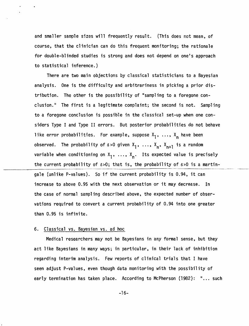
and smaller sample sizes will frequently result. (This does not mean, of

course, that the clinician can do this frequent monitoring; the rationale

for double-blinded studies is strong and does not depend on one's approach

to statistical inference.)

There are two main objections by classical statisticians to a Bayesian

analysis. One is the difficulty and arbitrariness in picking a prior dis­

tribution. The other is the possibility of "sampling to a foregone con­

clusion." The first is a legitimate complaint; the second is not. Sampling

to a foregone conclusion is possible in the classical set-up when one con­

siders Type I and Type II errors. But posterior probabilities do not behave

like error probabilities. For example, suppose x1, ... , Xn have been

observed. The probability of o>O given x1, ... , Xn, Xn+l is a random

variable when conditioning on x1, ... , Xn. Its expected value is precisely

the current probability of o>O; that is, the probability of o>O is a martin­

gale (unlike P-values). So if the current probability is 0.94, it can

increase to above 0.95 with the next observation or it may decrease. In

the case of normal sampling described above, the expected number of obser­

vations required to convert a current probability of 0.94 into one greater

than 0.95 is infinite.

6. Classical vs. Bayesian vs. ad hoc

Medical researchers may not be Bayesians in any formal sense, but they

act like Bayesians in many ways; in particular, in their lack of inhibition

regarding interim analysis. Few reports of clinical trials that I have

seen adjust P-values, even though data monitoring with the possibility of

early termination has taken place. According to McPherson (1982): 11 ••• such

-16-

arguments [for adjusting P-values] appear not to have captured the

imagination of the great majority of investigators." In fact, reports

of ongoing clinical trials are published with P-values calculated as

though the trial was fixed in size to be the current size.

Consider the following scenario. A medical researcher adopts a

sequential scheme--with normal observations, say. The researcher decides

to entertain up to 10 stages, stopping before with a two-sided significance

level of 0.05. The nominal P-value required is 0.0105. At the first

stage, Z = 2.559 (P = 0.0105) and so the trial was stopped, with the

researcher proclaiming P = 0.05.

While the results are being presented at a professional meeting, a

representative from the sponsoring agency states that the researcher was

not to receive funding beyond the first stage in any case. Does this

mean that, since the original intentions could not have been carried out,

Pis actually 0.0105?

Someone from another agency is in the audience and gets up to say

that they knew about the trial and the first agency's plan to withdraw

sponsorship. It seems they were willing to take over sponsorship for one

more stage should that have been necessary. Now, Pis neither 0.0105 nor

0.05, but 0.0185.

On the other hand, if the second agency had said they would have taken

over sponsorship only if the investigator would have agreed to up to 20

stages, then the P-value becomes >0.05 and the results are not significant!

Unless of course the researcher says he might not have agreed. What then

is the P-value?

-17-

The point of this story is to suggest that it is difficult if not

impossible to adher strictly to a classical approach. (Even more, as

Berger (1980, p. 354) says, "In a very strict sense, one wonders how the

classical statistician can do any analysis whatsoever.")

P-values (calculated assuming fixed sample sizes) may be reasonable

as measures of extremity, answering the question "How unusual are the

data?", but they should not be taken too seriously. The casual approach

employed by most researchers of reporting such P-values for the various

measurements (efficacy, safety, and side effects) is not without its

dangers. Consumers have to be educated to not necessarily act as though

H0

is false simply because Pis small. But adjusting P-values is even

less desirable, at least in part because it is so poorly understood by

the consumer. If the results of a trial are published then the reader

should be able to duplicate calculation of the given P-value without having

to know what the investigator would have done should various contingencies

have arisen.

Indeed, no investigator can specify all possible contingencies. The

statistician and the mode of inference must be flexible enough to handle

unforeseen developments. A remark of Cornfield in {Cutler, et al. 1966)

made in another context is appropriate here:

Of course a re-examination in the light of results of the assumptions on which the pre-observational partition of the sample space was based would be regarded in some circles as ~ad statistics. It would, however, be widely regarded as good science. I do not believe that anything that is good science can be bad statistics, and conclude my remarks with the hope that there are no statisticians so inflexible as

-18-

to decline to analyze an honest body of scientific data simply because it fails to conform to some favored theoretical scheme. If there are such, however, clinical trials, in my opinion, are not for them.

Acknowledgement. Chih-Kung Wu helped with the simulations reported

in Table 2.

-19-

REFERENCES

Anscombe, F. J., 1963. Sequential medical trials, J. Amer. Statist. Assoc. 58, 365-383.

Barnett, V., 1973 . Comparative Statistical Inference . John Wiley and Sons, London.

Berger, J. 0., 1980. Statistical Decision Theory , Foundat ions, Concepts, and Methods. Springer-Verlag, New York.

Berry, D. A., 1980. Statistical inference and the design of clinical tr ials. . Biomedicine R, 4-7.

Byar, D. P., Simon , R. M., Friedewald, W. T., Schlesselman, J . J., DeMets, D. L., Ellenberg, J . H., Gail, M. H., and vJare, J. H., 1976. Randomized clinical trials. New Engl. J. Med. 294, 74-80 .

C f . ld J 1966 Sequent,·a1 tr1·a1s, sequential analysis and the likelihood orn ,e , . , . principle. The Amer. Statist. 20, 18-23

Cutler, S. J., Greenhouse, S. W., Cornfield, J. and Schneiderman, M.A., 1966. The role of hypothes is testing in clinical t rials. J. Chron. Dis . ~, 857-882.

DeGroot, M. H., 1970 . Optimal Stat istical Decisions. McGraw-Hill, Inc., New York .

Diamond, G. A. and Forrester, J. S., 1983 . verdicts: Probable cause for appeal.

Clinical tri als and st~tist ical Ann. Internal Med. 98, 385-394.

Frei reich, E. J., Gehan, E., Frei, E., Schroeder, L. R., Wolman, I. J ., An bari, R., Burgert, E. 0., Mills, S. D., Pinkel, D., Selawry, 0. S., Moon, J. H., Gendel, B. R., Spurr, C. L., Storrs, R., Haura ni, F., Hoogstraten, B., and Lee, S., 1963. The effect of 6-Mercaptopurine on the duration of steroid-induced remissions in acute leukemia: A model for evaluation of other potentially useful therapy. Blood 21, 699-716. -

Jeffreys, H., 1961. Theory of Probability (3rd Ed. ) . Oxford University Press, London.

----- -

Lindgren, B. W., 1976. Statistical Theory 3rd Ed . Macmil l an Publishing Co . , Inc ., New York.

-20-

McPherson, K., 1982. On choosing the number of interim analyses in clinical trials. Statistics in Medicine l, 25-36.

Savage, L. J., 1954. The Foundations of Statistics. John Wiley and Sons, Inc., New York. (1972 edition, Dover Publications, New York.)

Simon, R., 1977. Adaptive treatment assignment methods and clinical trials. Biometrics 33, 743-749.

Tygstrup, N., Lachin, J.M., Juhl, E. {.eds.), 1982. The Randomized Clinical Trial and Therapeutic Decisions, Marcel Dekker, Inc., New York.

Weinstein, M. C., 1974. Allocations of subjects in medical experiments. New Engl. J. Med. 291, 1278-1285.

Winfrey, C., 1978 (March 5). The New York Times.

-21-