International Competition and Rent Sharing in French

Manufacturing

Lionel Nesta∗ Stefano Schiavo†

September, 2017

Preliminary and Incomplete

Abstract

The paper investigates the impact of import competition on rent sharing between firms

and employees. First, by applying recent advances in the estimation of price-costs margins

to a large panel of French manufacturing firms, we are able to classify each firm into six

different regimes based on the presence/absence of market power in both the labor and

product markets. Second, we concentrate on firms that operate in an efficient bargaining

framework to study the effect of import penetration on workers’ bargaining power. We find

that imports from OECD countries have a small negative effect, whereas Chinese competition

leads French firms to upgrade their products, and thus increases the bargaining power of

workers. Moreover, the effect is heterogeneous across firms, so that both the origin of imports

and firm-level characteristics play a role in determining the overall impact of international

competition. By providing firm-level evidence on the relationship between international trade

and rent sharing, the paper sheds new light on the effect of trade liberalization on the labor

market.

Keywords: firm heterogeneity; import competition; mark-up; wage bargaining;

JEL Classification: F14; F16; J50

∗GREDEG Universite Nice Sophia-Antipolis, OFCE SciencesPo and SKEMA Business School. E-mail: lio-nel.nesta@unice.fr

†University of Trento and OFCE SciencesPo. E-mail: stefano.schiavo@unitn.it

1 Introduction

The recent debate on the pros and cons of new (actual or potential) trade agreements and the

associated rise in protectionism sentiments (think of the recent withdrawal by the US from the

Trans-Pacific Partnership, the difficult ratification of the EU-Canada Free Trade Agreement, and

the dire state of negotiations on the Transatlantic Trade and Investment Partnership between

the EU and the US) have brought back on stage concerns about the effects of trade liberalization

on labor markets.

These concerns tend to be magnified when trade involves economies with different levels of

income per capita, social protection, and labor costs. In fact, the last two decades have witnessed

a very sharp increase in trade between OECD countries and emerging economies, due to the

rapid integration of some countries (most notably China) into world markets, falling trade costs

and the disintegration of production into several stages.

Such heated debates are likely to represent a recurrent theme in the near future, as other

emerging economies integrate into world markets and the (alleged) benefits of free trade are

further questioned. Hence, understanding how globalization affects European firms and workers

represents a crucial question both from an academic and a policy point of view.

Intuitively, we would expect increased competition from abroad to lower domestic firm’s

profit margins and, as a result, to lower the scope for rent sharing between firms and workers,

even in the context of highly regulated labor markets where direct effects on both employment

and wage levels might take time to materialize. On the other hand, some firms might respond

to price competition from emerging markets by improving product quality, moving upscale and

thus increase their price-cost margins. Hence, the impact of import competition on a firm’s

market power both in the product and in the labor markets may be heterogeneous and remains

an empirical issue.

In this paper we combine two streams of the recent empirical literature on market imperfecti-

ons to determine the product and labor market regimes in which firms operate. More specifically,

we build on the methodology developed by De Loecker & Warzynski (2012) to estimate producti-

vity and markups at firm level and combine the results with the approach used by Dobbelaere

& Mairesse (2013) and Dobbelaere et al. (2015) to classify sectors according to the (combined)

degree of product and labor market imperfections. In this way, we are able to classify firms

—not industries— into six different regimes depending on whether they enjoy market power on

the product and/or the labor market. To the best of our knowledge this is the first time that

such an exercise is performed at the firm level, and this represents the first contribution of the

paper.

Moreover, we investigate the relationship between our measure of workers’ bargaining power

and a number of firm-level characteristics, among which features the degree of import compe-

tition from both low-wage and industrial countries. In this way, we test the hypothesis that

import penetration acts as a disciplining device in wage bargaining, and we uncover signifi-

cant heterogeneity across firms. Such heterogeneity is important to analyze because in many

countries, and France is one of them, the system of collective bargaining often takes place at

2

the enterprise level, so that industry-level analysis may hide significant differences among firms

operating in the same sector.

The paper is organized as follows: the next section provides a quick overview of recent con-

tributions dealing with the effect of import competition on workers’ bargaining power. Section

3 describes the empirical methodology adopted to measure market imperfections, the data used,

and presents some descriptive results. In Section 4 we estimate the relationship between import

penetration and bargaining power using different econometric techniques. A discussion of the

results and some conclusions are then summarized in Section 5.

2 A glance at the existing literature

The impact of trade liberalization on labor market outcomes, such as wages and employment,

represents a classical research question in international economics. The literature has tackled it

from different angles, alternatively looking at developed or developing countries, wage levels or

wage inequality, skill premia vs unemployment. Early studies dating back to the 1990s tend to

find little direct effect of trade on labor market outcomes, and convey the broad message that

technical change plays a much more prominent role in explaining job losses and wage polariza-

tion in industrial countries. However, more recent studies that take into account outsourcing

and offshoring in addition to the standard import competition mechanism, tend to give more

relevance to trade-related explanations (Dumont et al. 2012). The effect of international trade

on workers’s bargaining power remains however a much less studied phenomenon. Moreover,

while a handful of studies exist on the subject, to the best of our knowledge, none of them has

ever addressed the issue at the firm level.

Dumont et al. (2006) analyze evidence for five European countries during 1994–1998. First

they estimate sector-level bargaining power from firm microdata, then they investigate its de-

terminant looking in particular at labor composition, R&D intensity, outsourcing practices,

market structure and imports from both OECD and emerging economies. For what concerns

trade variables, results suggest that only imports from OECD countries have a significant effect

on workers’ bargaining power.

A similar result emerges from a study on the UK performed by Boulhol et al. (2011). The

empirical approach is similar: the authors first estimate both markups and bargaining power

(by sector, year and size class), and then regress them on a series of covariates among which one

finds the share of imports from both industrial and developing countries in total demand. As

before, only imports from high-income countries seem to matter.1

Closer to our own approach, at least in spirit, is the work by Abraham et al. (2009) who ana-

lyze the price and wage setting behavior of Belgian manufacturing firms in the period 1996–2004,

and distinguish between import competition from four country groups, namely EU-15, new EU

members, other OECD countries, and the rest of the world. Their model assumes that increased

economic integration reduces firms’ price-cost margins and thus lowers the size of the rent to

share with workers. As a result, workers’ bargaining power is reduced. Although Abraham et al.

1Boulhol et al. (2011) assume that all firms/sectors are engaged in an efficient bargaining wage setting.

3

(2009) use firm-level data, they still assume that markups and bargaining power are the same

for all firms within the same industry. Their findings suggest that import competition puts

pressure on both markups and bargaining power, especially when there is increased competition

from low wage countries. The authors conclude that trade integration is associated with wage

moderation, which should then yield a positive effect on employment.

Moreno & Rodriguez (2011) address a similar question by looking at the hypothesis that

import reinforces market discipline both on product and labor markets. Using a small sample

of around 2,000 Spanish firms over the period 1990–2005 they look at both markups and bar-

gaining power, looking at whether import competition affects both the size of economic rents

(measured by the Lerner’s index) and their distribution between firms and workers. They find

a negative effect of import competition on the Lerner’s index, that is larger for firms producing

final goods. This is consistent with the notion that imports of final goods are more directly

in competition with domestic production and therefore put particular pressure on local firms.

From the point of view of rent sharing, Moreno & Rodriguez (2011) find that bargaining power

is smaller for producers of final and homogeneous goods. Interestingly, this paper presents a first

attempt to estimate markups at the firm level, applying the methodology developed by Roeger

(1995) (amended to allow for labor market imperfections as in Crepon et al. 2005) to each firm.

This implies running firm-level regressions that have between 9 and 15 observations each for a

subsample of 885 firms, and then focusing on the distribution of markups rather than on the

specific firm-level values.

An interesting extension to the standard theoretical setup that assumes homogeneity among

workers is offered by Dumont et al. (2012), who explicitly model bargaining between firms and

two types of unions, representing high- and low-skilled workers. The model’s implications are

then brought to the data using information on Belgian firms. The authors study the deter-

minants of bargaining power at sectoral level, and find that while the bargaining position of

high-skilled workers is not affected by either technical change or globalization, low-skilled wor-

kers are negatively affected by imports from non-OECD countries (where the wage differential

is likely to be larger), offshoring activities, and the presence of foreign affiliated in Central and

Easter European countries.

Two recent papers look at the effect of trade liberalization in India, thus taking the vintage

point of an emerging economy where market imperfection may be more relevant and where an

increase in (foreign) competition could trigger larger efficiency gains. Ahsan & Mitra (2014)

focus on the labor share of income following liberalization, but also report results on bargaining

power. They find that sectors featuring lower tariff rates before the liberalization display lower

bargaining power. Pal & Rathore (2016) exploit state-level variations in the deregulation of both

product and labor markets, and find that both types of reforms has led to significant declines in

workers’ bargaining power, while none of them has had any meaningful effect on firms’ price-cost

margins.

4

3 Empirical Strategy

3.1 Measuring Imperfect Markets

Dobbelaere & Mairesse (2013) show that in the context of a gross output production function

where factor inputs comprise labor, capital and materials, one can exploit the difference between

the markup computed on materials and labor to infer the existence of imperfect competition on

both the product and the labor market. The first important working assumption in this context

is that both labor (L) and materials (M) are variable inputs.2 The second key assumption of the

paper is to consider that materials prices PM equalize their marginal product. This assumption

allows us to consider the wedge between µMit and µLit as stemming from imperfections in the

labor market. In particular, Dobbelaere & Mairesse (2013) define a joint market imperfection

parameter:

Ψit =θMitαMit− θLitαLit

= µMit − µLit

whose sign and significance provides us with information on the presence of labor market im-

perfections. If all markets are perfects, the two terms on the right-hand side should amount

to unity. If the product market is imperfect but the two factor markets are perfect, then the

terms µMit and µLit must be strictly equal. Hence the left hand side term Ψit should be zero.

Based on our second working assumption, an inequality in µXit (Ψit 6= O) implies the presence of

imperfections in the labor market. Based on Hall (1988), Dobbelaere & Mairesse (2013) formally

show that Ψit informs us on three labor market regimes:

1. Efficient Bargaining (EB, Ψ > 0). Firms and risk-neutral workers bargain over wages and

employment level. In this case, it is possible to derive an expression for the absolute extent

of rent sharing (φit ∈ [0, 1]), i.e. the part of the rent that is appropriated by workers (with

1− φ being the share going to the firm).

2. Perfect competition - Right-to-manage (PR, Ψ = 0). In this case the labor market is coined

as operating under perfect competition, for neither the firms nor the workers can influence

wages.

3. Monopsony (MO, Ψ < 0). If firms enjoy monopsony power, we can derive measure of the

elasticity of labour supply with respect to wages βLS .

Exploiting the methodology presented above, we are able to obtain firm-level estimates of the

key parameters and therefore we can classify each firm in a different regime with the following

procedure. First, we compute the confidence intervals (CI) at 90% level for each firm-level

measure of µMit and µLit in a classical fashion (µXit < µXit ± z × σµX ,it) where X stands for either

M ort L, z = 1.64 and σµX ,it is given by:

2One could object that labour market is a quasi-variable input, especially in the case of France. However,incorporating it into the model is beyond the scope of the paper.

5

(σµX ,it)2 = (αXit )−2 ·

∑w

w2it · (σx)2 + 2 ·

∑x,z,x 6=z

xit · zit · covxz

where w = {1, l, k, lk} and x, z = {m, lm,mk, lmk} when X = M and w = {1,m, k,mk} and

x, z = {l, lm, lk, lmk} when X = L, where lower cases denote the log transformed variables of

capital K, labor L and materials M .

Second, and consistently with the above classification, the comparison of the two confidence

intervals allows us to classify the labor market in which each firm operates:

1. EB: Efficient Bargaining. If lower bound for the 90% CI µMit exceeds the upper bound of

the 90% CI for µitLM , then µMit is significantly greater than µLit: µMit > µLit ⇒ Ψit > 0, at

90% level.

2. PR: Perfect competition - Right-to-manage. If the two confidence intervals overlap, then

µMit is not significantly different from µLit: µMit = µLit ⇒ Ψit = 0, at 90% level.

3. MO: Monopsony. If lower bound for the 90% CI µLit exceeds the upper bound of the 90%

CI for µMit , then µMit is significantly lower than µLit: µMit < µLit ⇒ Ψit < 0, at 90% level.

Observe that to classify firms as operating under perfect or imperfect product market is now

straightforward. Using the confidence interval for µM , firms are coined as operating in perfect

markets if the lower bound of the 90% CI is below unity.

Based on the joint market imperfection parameter, Dobbelaere & Mairesse (2013) identify

six different regimes – each being a combination of the types of competition on both the product

and the labor market – in which they classify each industry (see Table 1). Results reported in

Section 3.3 suggest that there is substantial heterogeneity across firms operating in the same in-

dustry: therefore, the ability to account for the different behavior of firms represent an important

contribution of our work.

Table 1: Product and labor market regimes

product market

labor market perfect competition imperfect competition

perfect competition PC-PR IC-PRefficient bargaining PC-EB IC-EB

monopsony PC-MO IC-MO

3.2 Data

We use data on a large sample of French manufacturing firms based on the Enquete Annuelle

d’Entreprises (EAE), an annual survey that gathers balance sheets information for all manufac-

turing firms with at least 20 employees conducted until 2007 by the French Ministry of Industry.

The surveyed unit is the legal (not the productive) unit, which means that we are dealing with

6

firm-level data. We have data for the period 1993–2007, and after some basic cleaning from

outliers we have information for about 12,500 firms.3

Beside containing the main information from each firm’s income statement, the EAE also

reports some details on the different activities performed by firms: more specifically, it pro-

vides us a list of the 4-digit code of activities in which the firm is active, together with the

corresponding number of employees, sales and export. We use this information to derive the

relative importance of each activity within the firm and, by linking these weights to data on

imports retrieved from the BACI dataset maintained by CEPII (Guillaume Gaulier 2010) we

obtain a firm-specific measure of competition from low wage countries, from China, and from

OECD members.4 In this way we can exploit firm-specific heterogeneity in import competition,

that would otherwise be masked by the use of sector-level measures of import penetration. The

same source of data on each firm’s detailed activities is used to compute the share of employees

pertaining to high-tech activities within the firm.

Low-wage countries are defined following Bernard et al. (2006): a country is classified as

low-wage if its per capita GDP lower than 5% of the US value; our import competition measure

is the ratio of French imports (from any specific country or group of countries) over apparent

consumption in the same sector, i.e. total sales plus imports minus exports. Since trade data

are reported according to the HS classification while the EAE is based on the French industrial

classification system (NAF) we have developed a concordance between HS and NAF codes.

3.3 Descriptive Statistics

Tables 2 present information on the fraction of firm belonging to the six different market regimes

defined above by looking at the presence of product- and labor-market imperfections. Results

are based on a translog production function: Tables A2-A4 in the Appendix report analogous

results for the Cobb-Douglas specification and the OLS estimation of the trans-log production

function respectively, which are qualitatively similar.5

We see that there is substantial heterogeneity both across and within different sectors. Look-

ing at the whole economy, around 41% of firm-year observations fall within of the regimes classi-

fied as imperfect competition, meaning that the markup is significantly (from a statistical point

of view) but this fraction varies from a lower bound of less then 1% for Textiles to a higher

bound of almost 100% for Electric and electronic equipment and Printing and publishing.

For what concerns the labor market, efficient bargaining represent nearly 54% of firm-year

observations, followed by right-to-manage (37%) and monopsony, with less than 10% of obser-

vations. The single most common joint regime is the IC-EB combination, whereby firms enjoy

some degree of market power on both the product and labor market, and the rent is shared with

3We keep companies which are present at least 8 consecutive years and for which the annual growth ratesnever exceed ±100%.

4For more information on the BACI data, see http://www.cepii.fr/cepii/en/bdd_modele/presentation.

asp?id=15In the Cobb-Douglas specification the estimated output elasticities are constant within each sector, so that

all the firm-level heterogeneity in µL, µM and the associated parameters such as Ψ comes from variation in theinput shares αL and αM . In fact, Table A2 shows that firms are all classified as belonging to the EB labor marketregime.

7

Table 2: Percentage of firms in each market regime by sector: trans-log production function

Sector name ]Firm ]Obs. PC-PR PC-EB PC-MO IC-PR IC-EB IC-MO

C1 Clothing & footwear 1527 11062 57.32 19.27 2.67 1.53 17.12 2.09C2 Printing & publishing 1629 14346 0.81 0 0.09 7.58 91.02 0.50C3 Pharmaceuticals 555 4459 41.84 32.01 7.01 2.63 14.92 1.59C4 House equipm. & furnishings 1457 11622 23.03 25.30 2.035 2.65 44.52 2.46D0 Automobile 597 5085 61.56 22.44 5.30 1.10 9.15 0.45E1 Transportation machinery 332 2782 74.70 8.83 3.31 2.80 9.93 0.43E2 Machinery & mechanical equipm. 3694 31744 17.51 10.17 8.00 5.49 56.19 2.64E3 Electric & electronic equipm. 1198 9240 0.45 0 0.08 2.25 97.18 0.04F1 Mineral industries 904 7981 63.32 18.44 7.90 3.15 5.56 1.62F2 Textile 1254 10278 75.76 4.12 19.22 0.37 0.17 0.37F3 Wood & paper 1326 11581 57.91 15.58 16.33 1.33 5.72 3.13F4 Chemicals 2212 19301 19.63 19.63 3.22 4.33 51.38 1.81F5 Metallurgy, Iron & Steel 3881 34666 44.85 31.60 15.28 0.88 6.72 0.67F6 Electric & electronic comp. 960 7754 11.39 11.63 2.07 2.60 67.81 4.50

TOT All manufacturing 20622 181901 33.78 17.22 7.81 3.13 36.32 1.73

Product market regimes: PC = perfect competition; IC = imperfect competition.Labor market regimes: PR = perfect comp.; EB = efficient bargaining; MO = monopsony.

workers; this regime accounts for 36% of the sample, closely follows by the PC-PR group (close

to 34%) representing perfect competition in both labor and product markets.

It is worth noting that the relatively large standard errors associated with the fixed-effects

IV estimation of the production function results in wide confidence intervals for the the markup

µ and the joint market imperfection parameter Ψ: as a result, participation into the PC and

PR product- and labor-market regimes is somehow inflated since the confidence intervals often

include zero. In fact, OLS results (see Table A4), which are characterized by lower standard

errors (although plagued by endogeneity issues) suggest that a much smaller faction of firms

operates in perfect competition.

Table 2 suggests the presence of widespread variations also within each sector. In fact, while

in most of the sectors it is possible to identify a prominent regime, in several cases, there at

least a second, and often a third, relevant regime that covers a significant fraction of firm-year

observations. Hence, characterizing all firms within a sector as belonging to the same regime

would imply a significant loss of information and would hide substantial heterogeneity. For

instance, 57.32% of the observations within Clothing and Footwear are classified as PC-PR,

while 17.12% belong to the IC-EB regime and another 19.27% to PC-EB. In Metallurgy, Iron

and Steel the most common regime (PC-PR) covers 45% of observations, 32% are classified as

PC-EB and 15% as PC-MO.

Table 3 summarizes the mean values of the key parameters by industry and for the overall

sample of manufacturing firms. The average markup charged by French firms is around 11%,

ranging between a 10% markdown (a markup lower than 1, see for instance Caselli et al. 2017 for

an investigation of this phenomenon) in the textile sector, to a hefty 64% in electric and electronic

equipment. Within each sector there is however a substantial difference between firms that

have significant market power (i.e. they operate in imperfect competition) and those for which

the price is not significantly different from the marginal cost. Columns (2) and (3) highlight

8

this difference and show that firms classified as price takers have markups not significantly

different from 1, while the remaining group manages to charge markups that range between

16% (machinery and mechanical equipment) and 68% (electric and electronic equipment).

Turning to labor market regimes, we see that the share of economic rent that goes to labor

(φ) in the efficient bargaining setting is around 55% (with some variability across sectors, the

min/max values are 48% and 68%). On the other hand, the wage elasticity of labor supply dis-

plays substantial variation across industries and is associated with varying degrees of monopsony

power.

Table 3: Mean values of key parameters by industry: trans-log production function

(1) (2) (3) (4) (5) (6) (7) (8) (9)overall PC IC efficient bargaining monopsony

sector µ µ µ Ψ γ φ Ψ β εLs

w

C1 1.192 1.141 1.419 0.522 2.808 0.619 -0.395 0.709 2.672C2 1.454 0.995 1.469 0.667 2.514 0.602 -0.472 0.730 3.168C3 1.160 1.076 1.563 0.714 2.104 0.559 -0.664 0.579 1.412C4 1.127 1.022 1.284 0.470 2.386 0.591 -0.400 0.702 2.708D0 1.017 0.980 1.347 0.446 2.395 0.591 -0.397 0.685 2.305E1 1.118 1.067 1.469 0.648 2.079 0.587 -0.682 0.578 1.466E2 1.078 0.961 1.164 0.348 1.818 0.527 -0.235 0.807 5.349E3 1.642 1.007 1.675 0.973 3.409 0.684 -0.540 0.682 2.322F1 0.994 0.963 1.286 0.360 1.706 0.506 -0.327 0.722 2.851F2 0.899 0.894 1.434 0.366 2.093 0.523 -0.376 0.673 2.230F3 0.976 0.950 1.218 0.401 1.533 0.493 -0.383 0.690 2.457F4 1.096 0.979 1.223 0.417 1.694 0.505 -0.319 0.756 3.583F5 0.933 0.910 1.190 0.255 1.471 0.484 -0.246 0.772 4.084F6 1.205 1.030 1.302 0.584 2.475 0.600 -0.481 0.682 2.592

Total 1.110 0.974 1.323 0.477 2.085 0.553 -0.288 0.750 3.761

µ: markup, Ψ: joint market imperfection; φ: absolute rent sharing; γ = φ/(1 − φ):relative rent sharing; εL

s

w : wage elasticity of the labor supply; β = εLs

w /(1 − εLs

w ):degree of monopsony power.

3.4 Econometric specification

The spirit of the empirical specification we develop in this paper is to allow for the effect of

import penetration on rent sharing φ to be different according to the degree of market power

enjoyed by firms on the product (as captured by µ). In fact, we hypothesize that the degree of

rent sharing will depend on the size of the economic rent that the firm is able to generate. The

baseline model can be seen as an adaptation of the standard empirical specification which reads

as:

φit+1 = β0 + β1IMP sit + β2εµit + BX + νi + λt + eit, (1)

where IMP sit is import penetration from source country s. Importantly, import penetration is

firm-year specific because we make use of firm sales by industry at the four digit level:

9

IMP sit =∑k

(Sdikt0 ×

IMP sktIMPkt

)(2)

where k identifies all the different industrial sectors in which firm i is active, Sdikt0 represents

their individual share in domestic sales in 1994 (the year before our analysis starts, or in the first

year in which the firm enters the sample), and IMP skt denotes imports from country s in sector

k at time t. Hence, the import competition measure has features a firm-level heterogeneity that

comes from the portfolio of activities of each firm, while its variation over time depends on

industry-level imports. In this way we minimize endogeneity concerns.

The variable εµit captures market power in the product market, net of industry structure and

costs. More specifically, it is computes as the residual (plus the constant term) of a regression of

the mark-up µ on a polynomial of over five comprising average costs, the number of firms active

in the main sector of activity of the firm, and the Herfindahl index for sales (net of firm i). This

variable is meant to capture the degree of market power of each firm that is due to firm-specific

characteristics —such as quality or brand power– and not depending on the industry structure.

X is a vector of additional controls which includes productivity ω, firm size s, employment

growth at the local (NUTS 3) level to control for the tightness of the labor market; νi and λt

are firm i and time t effects and eit is the error term. Observe that rent sharing φ, import

penetration IMP , product market power εµ all vary across firms and years. The parameters of

interest is β1, that is, the effect of foreign competition on rent sharing.

To allow for an heterogeneous effect of import penetration IMP on φ, a natural point of

departure is to argue that the latter depends on product quality —that is, εµit – and therefore

to interact IMP with εµit, yielding the following model:

φit+1 = β0 + β1IMPit + β2εµit + β3IMPit × µit + BX + νi + λt + eit, (3)

In this setting, the marginal effect of IMP on φ depends on εµit, that is, ∂φ/∂IMP =

β1 + β3 · εµit.Following a common strategy in the recent (Autor et al. 2013, Hummels et al. 2014, Ashournia

et al. 2014, see for instance), we instrument import competition to account for a possible omitted

variable bias stemming from factors that simultaneously affect both French imports and a firm’s

bargaining power vis-a-vis its workers. In equation (2), French imports from source country s

in any given 4-digit sector k are then substituted with country s exports to all other counties

minus France.6

6Similar results are obtained using a limited number of non-EU countries, as done by Dauth et al. (2014).

10

4 Empirical Results

4.1 International Competition and Rent Sharing

[TO BE COMPLETED]

Table 4: Rent Sharing as a function of International Competition.Sequential Regressions. Dependent Variable: Rent Sharing φ.

(1) (2) (3) (4) (5) (6) (7)

Import Penetration China 0.287*** 0.309*** 0.310*** 0.204* 1.226*** 0.294*** 1.555***(0.089) (0.090) (0.090) (0.108) (0.340) (0.106) (0.392)

Import Penetration OECD -0.006 -0.016* -0.017** -0.009 -0.015* 0.023 0.096***(0.008) (0.008) (0.008) (0.009) (0.008) (0.029) (0.036)

Productivity ω -0.056*** -0.056*** -0.066*** -0.064*** -0.059*** -0.067***(0.008) (0.008) (0.009) (0.009) (0.008) (0.009)

Size (Log of employment) 0.023*** 0.023*** 0.016*** 0.017*** 0.022*** 0.015**(0.006) (0.006) (0.006) (0.006) (0.006) (0.006)

Employment Growth (NUTS 3) 0.007** 0.004 0.004 0.006* 0.003(0.003) (0.003) (0.003) (0.003) (0.003)

Markup residual εµ 0.182*** 0.201*** 0.075* 0.358***(0.059) (0.064) (0.042) (0.097)

Mill’s Ratio 0.020*** 0.024*** 0.025*** -0.043* -0.036* 0.009 -0.058**(0.004) (0.004) (0.004) (0.022) (0.019) (0.010) (0.023)

IMP China ×εµ -0.961*** -1.333***(0.350) (0.417)

IMP OECD ×εµ -0.036 -0.107***(0.027) (0.034)

Observations 49,480 49,480 49,480 49,480 49,468 49,468 49,468R-squared 0.043 0.047 0.047 0.048 0.048 0.048 0.049Number of firms 9,198 9,198 9,198 9,198 9,198 9,198 9,198Weak ID Kleibergen-Paap 472.5 473.7 473.7 456.2 116.2 248.0 53.99Number of exclusion restrictions 2 2 2 2 3 3 4RMSE 0.123 0.123 0.123 0.123 0.123 0.123 0.123

Clustered standard errors in parentheses. *** p<0.01, ** p<0.05, * p<0.1. All regressions include a full vector of unreportedyear fixed effects.

11

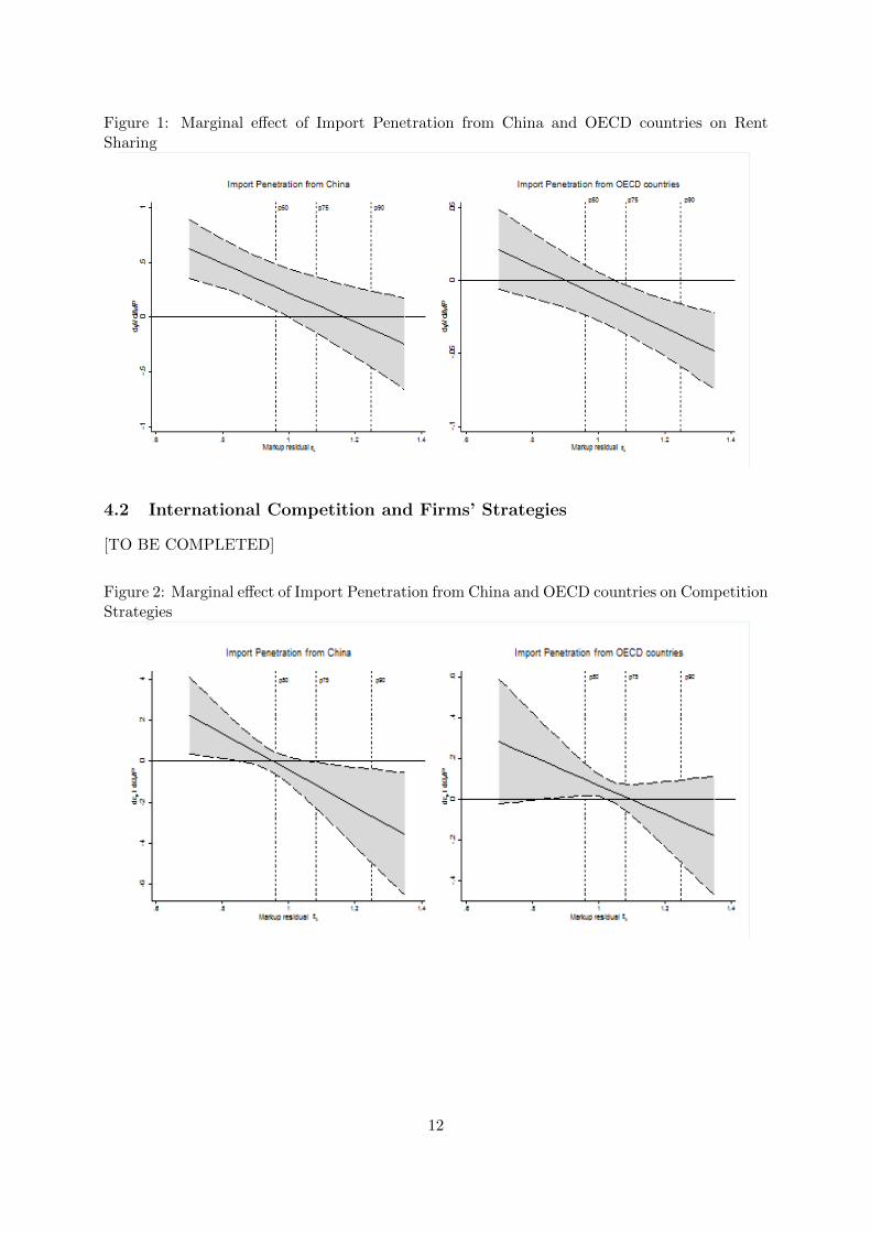
Figure 1: Marginal effect of Import Penetration from China and OECD countries on RentSharing

4.2 International Competition and Firms’ Strategies

[TO BE COMPLETED]

Figure 2: Marginal effect of Import Penetration from China and OECD countries on CompetitionStrategies

12

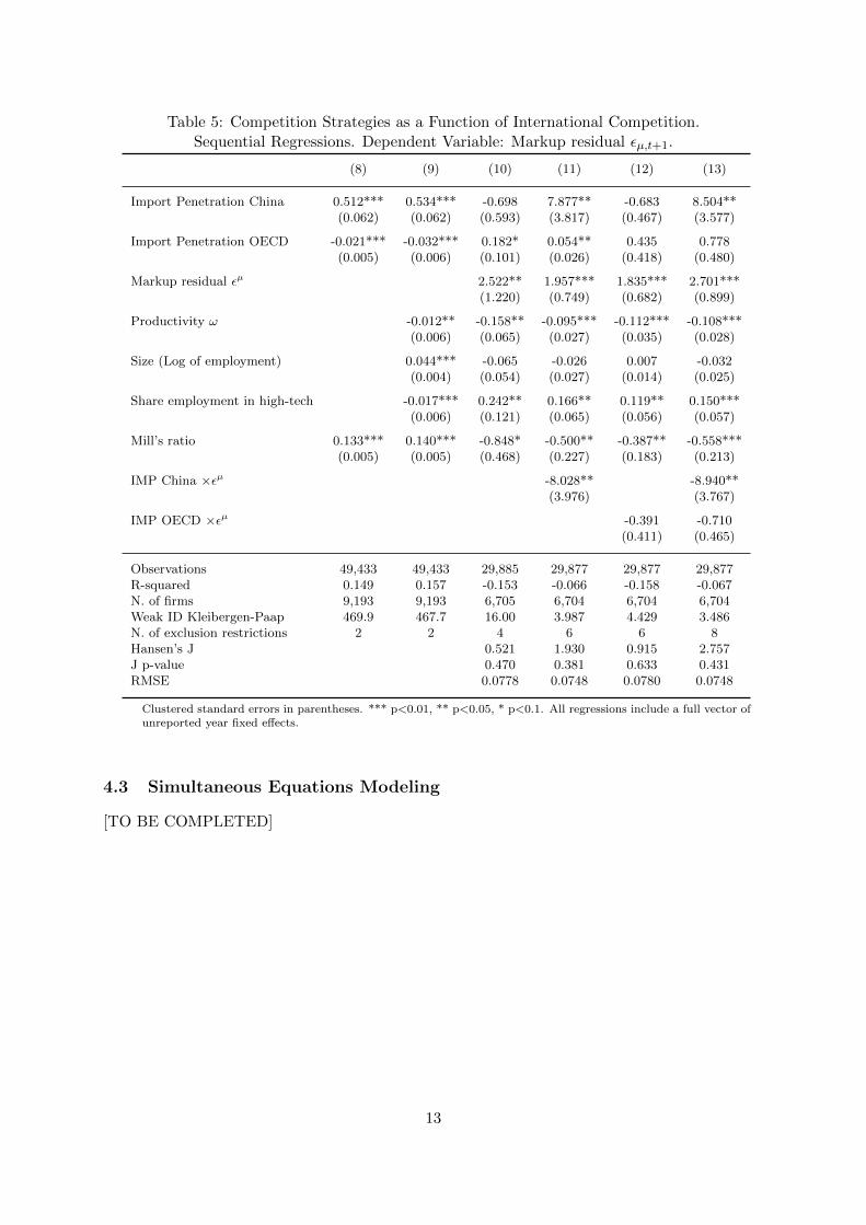
Table 5: Competition Strategies as a Function of International Competition.Sequential Regressions. Dependent Variable: Markup residual εµ,t+1.

(8) (9) (10) (11) (12) (13)

Import Penetration China 0.512*** 0.534*** -0.698 7.877** -0.683 8.504**(0.062) (0.062) (0.593) (3.817) (0.467) (3.577)

Import Penetration OECD -0.021*** -0.032*** 0.182* 0.054** 0.435 0.778(0.005) (0.006) (0.101) (0.026) (0.418) (0.480)

Markup residual εµ 2.522** 1.957*** 1.835*** 2.701***(1.220) (0.749) (0.682) (0.899)

Productivity ω -0.012** -0.158** -0.095*** -0.112*** -0.108***(0.006) (0.065) (0.027) (0.035) (0.028)

Size (Log of employment) 0.044*** -0.065 -0.026 0.007 -0.032(0.004) (0.054) (0.027) (0.014) (0.025)

Share employment in high-tech -0.017*** 0.242** 0.166** 0.119** 0.150***(0.006) (0.121) (0.065) (0.056) (0.057)

Mill’s ratio 0.133*** 0.140*** -0.848* -0.500** -0.387** -0.558***(0.005) (0.005) (0.468) (0.227) (0.183) (0.213)

IMP China ×εµ -8.028** -8.940**(3.976) (3.767)

IMP OECD ×εµ -0.391 -0.710(0.411) (0.465)

Observations 49,433 49,433 29,885 29,877 29,877 29,877R-squared 0.149 0.157 -0.153 -0.066 -0.158 -0.067N. of firms 9,193 9,193 6,705 6,704 6,704 6,704Weak ID Kleibergen-Paap 469.9 467.7 16.00 3.987 4.429 3.486N. of exclusion restrictions 2 2 4 6 6 8Hansen’s J 0.521 1.930 0.915 2.757J p-value 0.470 0.381 0.633 0.431RMSE 0.0778 0.0748 0.0780 0.0748

Clustered standard errors in parentheses. *** p<0.01, ** p<0.05, * p<0.1. All regressions include a full vector ofunreported year fixed effects.

4.3 Simultaneous Equations Modeling

[TO BE COMPLETED]

13

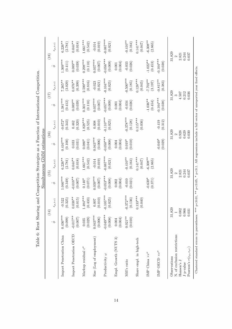
Tab

le6:

Ren

tS

har

ing

and

Com

pet

itio

nS

trat

egie

sas

aF

un

ctio

nof

Inte

rnat

ion

alC

omp

etit

ion

.S

imu

ltan

eou

sG

MM

esti

mat

ion

s

(14)

(15)

(16)

(17)

(18)

φε µ,t+1

φε µ,t+1

φε µ,t+1

φε µ,t+1

φε µ,t+1

Imp

ort

Pen

etra

tion

Chin

a0.4

36***

-0.5

22

1.0

46***

6.2

26**

0.4

16***

-0.6

72*

1.3

81***

7.2

65**

1.3

69***

6.2

26**

(0.0

99)

(0.3

25)

(0.3

49)

(2.7

81)

(0.1

00)

(0.3

43)

(0.4

12)

(3.0

29)

(0.4

11)

(2.7

81)

Imp

ort

Pen

etra

tion

OE

CD

-0.0

17**

0.0

38**

-0.0

18**

0.0

44**

0.0

33

0.4

62

0.0

89**

0.8

76**

0.0

89**

0.0

44**

(0.0

07)

(0.0

15)

(0.0

07)

(0.0

18)

(0.0

31)

(0.3

20)

(0.0

39)

(0.3

99)

(0.0

39)

(0.0

18)

Mark

up

resi

dualεµ

0.0

35

1.4

84***

0.1

40*

1.6

61***

0.0

80*

1.8

28***

0.3

01***

2.5

90***

0.2

98***

1.6

61***

(0.0

29)

(0.4

33)

(0.0

71)

(0.5

42)

(0.0

41)

(0.5

25)

(0.1

10)

(0.8

16)

(0.1

10)

(0.5

42)

Siz

e(L

og

of

emplo

ym

ent)

0.0

43***

0.0

07

0.0

39***

-0.0

14

0.0

43***

0.0

08

0.0

37***

-0.0

23

0.0

37***

-0.0

14

(0.0

06)

(0.0

10)

(0.0

07)

(0.0

19)

(0.0

06)

(0.0

10)

(0.0

07)

(0.0

21)

(0.0

07)

(0.0

19)

Pro

duct

ivit

yω

-0.0

49***

-0.1

05***

-0.0

53***

-0.0

87***

-0.0

50***

-0.1

10***

-0.0

57***

-0.1

04***

-0.0

56***

-0.0

87***

(0.0

08)

(0.0

25)

(0.0

08)

(0.0

21)

(0.0

08)

(0.0

25)

(0.0

09)

(0.0

25)

(0.0

09)

(0.0

21)

Em

pl.

Gro

wth

(NU

TS

3)

0.0

04

0.0

02

0.0

04

0.0

01

0.0

01

(0.0

04)

(0.0

04)

(0.0

04)

(0.0

04)

(0.0

04)

Mill’s

rati

o0.0

21**

-0.3

72***

-0.0

10

-0.4

10**

0.0

19*

-0.3

78***

-0.0

34

-0.5

00***

-0.0

33

-0.4

10**

(0.0

10)

(0.1

36)

(0.0

21)

(0.1

64)

(0.0

10)

(0.1

28)

(0.0

26)

(0.1

85)

(0.0

26)

(0.1

64)

Share

empl.

inhig

h-t

ech

0.1

33***

0.1

41***

0.1

15***

0.1

28***

0.1

41***

(0.0

40)

(0.0

47)

(0.0

36)

(0.0

45)

(0.0

47)

IMP

Chin

a×εµ

-0.6

39*

-6.3

08**

-1.0

36**

-7.7

02**

-1.0

22**

-6.3

08**

(0.3

71)

(2.8

65)

(0.4

54)

(3.1

97)

(0.4

53)

(2.8

65)

IMP

OE

CD

×εµ

-0.0

49*

-0.4

19

-0.1

04***

-0.8

15**

-0.1

04***

(0.0

29)

(0.3

12)

(0.0

38)

(0.3

83)

(0.0

38)

Obse

rvati

ons

31,8

29

31,8

29

31,8

29

31,8

29

31,8

29

N.

of

excl

usi

on

rest

rict

ions

12

23

2H

anse

n’s

J0.0

02

2.8

21

0.9

28

4.5

07

2.8

21

Jp-v

alu

e0.9

66

0.2

44

0.6

29

0.2

12

0.2

44

Pea

rson’sr(ε φ,εεµ

)0.0

31

0.0

37

0.0

30

0.0

36

0.0

37

Clu

ster

edst

an

dard

erro

rsin

pare

nth

eses

.***

p<

0.0

1,

**

p<

0.0

5,

*p<

0.1

.A

llre

gre

ssio

ns

incl

ud

ea

full

vec

tor

of

un

rep

ort

edyea

rfi

xed

effec

ts.

14

5 Conclusion

This paper combines recent advances in the estimation of firm-level markups to classify firms

into six different regimes based on the presence of imperfections in both the product and labor

market. Using a large sample of French manufacturing firms we show that there is substantial

heterogeneity in firm behavior both across and within industries, so that being able to properly

account for firm-level differences provides us with relevant information.

The methodology adopted in the paper allows us to estimate a measure of workers’ bargai-

ning power, that we relate to measures of import competition to investigate how globalization

affects rent sharing, while controlling for a number of firm-level characteristics such as average

costs, productivity and size. We find that import competition has an heterogeneous effect on

workers’ bargaining power depending both on the source of imports and the characteristics of

the firm. We find three main results: i) import from OECD countries is negatively correlated

with the share of economic rent going to workers; ii) competition from China, on the contrary, is

positively associated with bargaining power. We interpret this result as suggesting that French

manufacturing firms has attempted to escape this type of competition by moving upscale and

improving the quality of their products. Indeed, we find that iii) the impact of Chinese compe-

tition depends on the quality of the products sold by firms, and its effects are stronger for firms

in the lower end of the quality ladder.

The methodology presented in the paper lends itself to several different applications: in

particular, the possibility to link firm-level results with detailed information on employees (e.g.

their composition in terms of occupations, skills, educational attainments) represents an ideal

extension of the work that we would like to pursue in the future.

Acknowledgments

The authors blame each other for any remaining mistake. They thank Mauro Caselli, Michele Cascarano,

Sabien Dobbelaere, Nazanin Behzadan, and participants to the Workshop on Markups and Misallocations

(Trento), the 8th Rocky Mountain Empirical Trade Conference (Banff), the XVIII Conference in Inter-

national Economics (La Rabida, Huelva), the 2016 ISGEP meeting in Pescara, the XXXI AIEL National

Conference (Trento), for useful discussion.

15

References

Abraham, F., Konings, J. & Vanormelingen, S. (2009), ‘The effect of globalization on union

bargaining and price-cost margins of firms’, Review of World Economics (Weltwirtschaftliches

Archiv) 145(1), 13–36.

Ackerberg, D. A., Caves, K. & Frazer, G. (2015), ‘Identification properties of recent production

function estimators’, Econometrica 83(6), 2411–2451.

Ahsan, R. N. & Mitra, D. (2014), ‘Trade liberalization and labor’s slice of the pie: Evidence

from Indian firms’, Journal of Development Economics 108(C), 1–16.

Ashournia, D., Munch, J. & Nguyen, D. (2014), The Impact of Chinese Import Penetration

on Danish Firms and Workers, Economics Series Working Papers 703, University of Oxford,

Department of Economics.

Autor, D. H., Dorn, D. & Hanson, G. H. (2013), ‘The China Syndrome: Local Labor Market Ef-

fects of Import Competition in the United States’, American Economic Review 103(6), 2121–

2168.

Bernard, A. B., Jensen, J. B. & Schott, P. K. (2006), ‘Survival of the best fit: Exposure to

low-wage countries and the (uneven) growth of U.S. manufacturing plants’, Journal of Inter-

national Economics 68(1), 219–237.

URL: https://ideas.repec.org/a/eee/inecon/v68y2006i1p219-237.html

Boulhol, H., Dobbelaere, S. & Maioli, S. (2011), ‘Imports as Product and Labour Market Dis-

cipline’, British Journal of Industrial Relations 49(2), 331–361.

Caselli, M., Schiavo, S. & Nesta, L. (2017), Markups and markdowns, Working Paper 2017-11,

Sciences Po OFCE.

Crepon, B., Desplatz, R. & Mairesse, J. (2005), ‘Price-Cost Margins and Rent Sharing: Evi-

dence from a Panel of French Manufacturing Firms’, Annals of Economics and Statistics

(79-80), 583–610.

Dauth, W., Findeisen, S. & Suedekum, J. (2014), ‘The Rise Of The East And The Far East: Ger-

man Labor Markets And Trade Integration’, Journal of the European Economic Association

12(6), 1643–1675.

De Loecker, J. & Warzynski, F. (2012), ‘Markups and Firm-Level Export Status’, American

Economic Review 102(6), 2437–71.

URL: https://ideas.repec.org/a/aea/aecrev/v102y2012i6p2437-71.html

Dobbelaere, S., Kiyota, K. & Mairesse, J. (2015), ‘Product and labor market imperfections

and scale economies: Micro-evidence on France, Japan and the Netherlands’, Journal of

Comparative Economics 43(2), 290–322.

URL: https://ideas.repec.org/a/eee/jcecon/v43y2015i2p290-322.html

16

Dobbelaere, S. & Mairesse, J. (2013), ‘Panel data estimates of the production function and

product and labor market imperfections’, Journal of Applied Econometrics 28(1), 1–46.

URL: https://ideas.repec.org/a/wly/japmet/v28y2013i1p1-46.html

Dumont, M., Rayp, G. & Willeme, P. (2006), ‘Does internationalization affect union bargaining

power? An empirical study for five EU countries’, Oxford Economic Papers 58(1), 77–102.

Dumont, M., Rayp, G. & Willeme, P. (2012), ‘The bargaining position of low-skilled and high-

skilled workers in a globalising world’, Labour Economics 19(3), 312–319.

Guillaume Gaulier, S. Z. (2010), BACI: International trade database at the product-level. the

1994-2007 version, Working Paper 2010-23, CEPII.

Hall, R. (1988), ‘The relationship between price and marginal cost in US industry’, Journal of

Political Economy 95(5), 921–947.

Hall, R. E. (1986), ‘Market structures and macroeconomic fluctuations’, Brookings Papers on

Economic Activity pp. 285–322.

Hummels, D., Jørgensen, R., Munch, J. R. & Xiang, C. (2014), ‘The Wage Effects of Offs-

horing: Evidence from Danish Matched Worker-Firm Data’, American Economic Review

104(6), 1597–1629.

Levinsohn, J. & Petrin, A. (2003), ‘Estimating Production Functions Using Inputs to Control

for Unobservables’, Review of Economic Studies 70(2), 317–341.

URL: https://ideas.repec.org/a/oup/restud/v70y2003i2p317-341.html

Moreno, L. & Rodriguez, D. (2011), ‘Markups, bargaining power and offshoring: An empirical

assessment1’, The World Economy 34(9), 1593–1627.

Pal, R. & Rathore, U. (2016), ‘Estimating workers’ bargaining power and firms’ markup in India:

Implications of reforms and labour regulations’, Journal of Policy Modeling 38(6), 1118–1135.

Roeger, W. (1995), ‘Can imperfect competition explain the difference between primal and dual

productivity measures ? estimates for U.S. manufacturing’, Journal of Political Economy

103, 316–330.

Wooldridge, J. M. (2009), ‘On estimating firm-level production functions using proxy variables

to control for unobservables’, Economics Letters 104(3), 112–114.

URL: https://ideas.repec.org/a/eee/ecolet/v104y2009i3p112-114.html

17

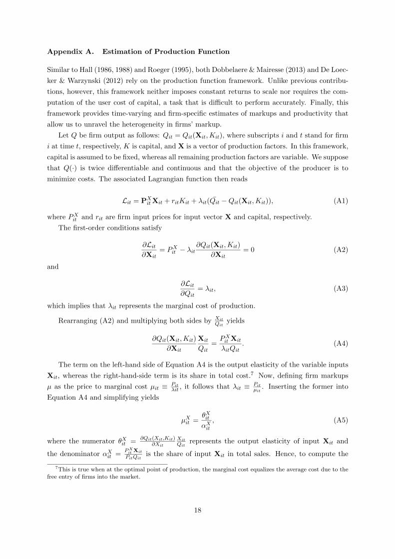
Appendix A. Estimation of Production Function

Similar to Hall (1986, 1988) and Roeger (1995), both Dobbelaere & Mairesse (2013) and De Loec-

ker & Warzynski (2012) rely on the production function framework. Unlike previous contribu-

tions, however, this framework neither imposes constant returns to scale nor requires the com-

putation of the user cost of capital, a task that is difficult to perform accurately. Finally, this

framework provides time-varying and firm-specific estimates of markups and productivity that

allow us to unravel the heterogeneity in firms’ markup.

Let Q be firm output as follows: Qit = Qit(Xit,Kit), where subscripts i and t stand for firm

i at time t, respectively, K is capital, and X is a vector of production factors. In this framework,

capital is assumed to be fixed, whereas all remaining production factors are variable. We suppose

that Q(·) is twice differentiable and continuous and that the objective of the producer is to

minimize costs. The associated Lagrangian function then reads

Lit = PXitXit + ritKit + λit(Qit −Qit(Xit,Kit)), (A1)

where PXit and rit are firm input prices for input vector X and capital, respectively.

The first-order conditions satisfy

∂Lit∂Xit

= PXit − λit∂Qit(Xit,Kit)

∂Xit= 0 (A2)

and

∂Lit∂Qit

= λit, (A3)

which implies that λit represents the marginal cost of production.

Rearranging (A2) and multiplying both sides by XitQit

yields

∂Qit(Xit,Kit)

∂Xit

Xit

Qit=PXit Xit

λitQit. (A4)

The term on the left-hand side of Equation A4 is the output elasticity of the variable inputs

Xit, whereas the right-hand-side term is its share in total cost.7 Now, defining firm markups

µ as the price to marginal cost µit ≡ Pitλit , it follows that λit ≡ Pit

µit. Inserting the former into

Equation A4 and simplifying yields

µXit =θXitαXit

, (A5)

where the numerator θXit = ∂Qit(Xit,Kit)∂Xit

XitQit

represents the output elasticity of input Xit and

the denominator αXit =PXit Xit

PitQitis the share of input Xit in total sales. Hence, to compute the

7This is true when at the optimal point of production, the marginal cost equalizes the average cost due to thefree entry of firms into the market.

18

markup µit, we need to compute both θXit and αXit per firm and per time period. Although it is

straightforward to compute αXit , the estimation of θXit is more demanding.

At the outset, two important choices need to be made explicit. First, we limit the set

of variable inputs to labor L and M . Theoretically, if all factor markets were perfect, the

markup derived from material must yield the same value as the markup derived from labor:

µMit = µLit. However, differences in factor markets’ imperfections will yield different values of

firm markups (µMit 6= µLit). Hence the wedge between µMit and µLit will be used to infer factor

market imperfections. This also implies that we define output Q as gross output.

The second important choice involves the functional form of Q(·). The most common can-

didate is the Cobb-Douglas framework. This functional form would yield an estimate of the

output elasticity of labor that would be common to the set of firms to which the estimation

pertains: θLit = θL, hence, θLit = θLjt for all firms i and j, i 6= j, included in the estimation sample.

It follows that the heterogeneity of firm markups and the ratio of the output elasticity of labor

on its revenue share would simply reflect heterogeneity in the revenue share of labor: µLit = θX

αLit.

Therefore, we prefer to use the translog production function because it generates markups whose

distribution is not solely determined by heterogeneity in the revenue share of labor, as will be

clear below.

Several different methods exists to estimate the production function. Here we follow Wool-

dridge (2009), i.e. a modification of the approach proposed by Levinsohn & Petrin (2003) and

Ackerberg et al. (2015) to control for unobserved productivity shocks using intermediate inputs.

Wooldridge (2009) proposes a joint estimation method that sidesteps some of the drawbacks

associated with the the control function (two-step) procedures and leads to more efficient esti-

mators. Table A1 reports the estimated output elasticities of the three production factors K,

L and M using the Cobb-Douglas and the preferred translog specifications. We also report the

estimated scale factor η computed as the sum of the three output elasticities η = θK + θL + θM .

19

Tab

leA

1:

Ou

tpu

tE

last

icit

iesθ

forK

,L

andM

and

the

corr

esp

ond

ing

scal

eec

onom

iesη.

Cob

b-D

ougla

san

dT

ran

slog

spec

ifica

tion

su

sin

gth

eW

ool

dri

dge

esti

mat

or.

Indust

ry]

Obs.

αL

αM

θK cd

θL cd

θM cd

ηcd

θK tl

θL tl

θM tl

ηtl

All

manufa

cturi

ng

181,9

01

0.3

31

0.6

13

0.0

68

0.2

28

0.6

32

0.9

28

0.0

71

0.2

68

0.6

30

0.9

69

Auto

mobile

5,0

85

0.2

62

0.7

03

0.0

71

0.1

65

0.6

74

0.9

10

0.0

66

0.2

01

0.6

84

0.9

51

Chem

icals

19,3

01

0.2

64

0.6

81

0.0

84

0.1

61

0.6

90

0.9

34

0.0

65

0.1

95

0.7

20

0.9

80

Clo

thin

gand

footw

ear

11,0

62

0.4

50

0.5

12

-0.0

10

0.2

72

0.7

77

1.0

39

0.0

98

0.4

05

0.5

37

1.0

41

Ele

ctri

cand

Ele

ctro

nic

com

ponen

ts7,7

54

0.3

27

0.6

17

0.0

50

0.2

16

0.6

41

0.9

07

0.0

22

0.2

29

0.7

11

0.9

62

Ele

ctri

cand

Ele

ctro

nic

equip

men

t9,2

40

0.3

72

0.5

85

-0.0

28

0.2

27

0.8

62

1.0

61

-0.0

37

0.2

43

0.8

37

1.0

43

House

equip

men

tand

furn

ishin

gs

11,6

22

0.3

37

0.6

35

0.0

86

0.2

26

0.6

10

0.9

22

0.0

76

0.2

46

0.6

82

1.0

03

Mach

iner

yand

mec

hanic

al

equip

men

t31,7

44

0.3

35

0.6

16

0.0

58

0.2

63

0.6

05

0.9

26

0.0

56

0.2

82

0.6

43

0.9

82

Met

allurg

y,Ir

on

and

Ste

el34,6

66

0.3

53

0.5

74

0.1

18

0.2

36

0.5

15

0.8

69

0.1

20

0.2

94

0.4

96

0.9

11

Min

eral

indust

ries

7,9

81

0.3

14

0.6

37

0.0

94

0.2

32

0.5

91

0.9

18

0.1

14

0.2

56

0.5

94

0.9

63

Pharm

ace

uti

cals

4,4

59

0.2

39

0.6

77

0.0

47

0.0

97

0.8

73

1.0

17

0.0

67

0.1

48

0.7

46

0.9

61

Pri

nti

ng

and

publish

ing

14,3

46

0.3

45

0.5

76

-0.0

05

0.2

53

0.7

68

1.0

17

-0.0

08

0.2

75

0.7

73

1.0

40

Tex

tile

10,2

78

0.3

32

0.6

12

0.1

46

0.2

21

0.4

25

0.7

92

0.1

37

0.2

95

0.4

86

0.9

18

Tra

nsp

ort

ati

on

mach

iner

y2,7

82

0.3

37

0.6

16

0.0

84

0.2

78

0.5

89

0.9

51

0.0

89

0.2

96

0.6

54

1.0

40

Wood

and

pap

er11,5

81

0.2

76

0.6

71

0.0

66

0.2

24

0.6

02

0.8

92

0.0

67

0.2

60

0.6

26

0.9

53

Su

per

crip

tcd

stan

ds

for

the

Cob

b-D

ou

gla

ssp

ecifi

cati

on

.S

up

ersc

rip

ttl

stan

ds

for

the

tran

slog

spec

ifica

tion

.

20

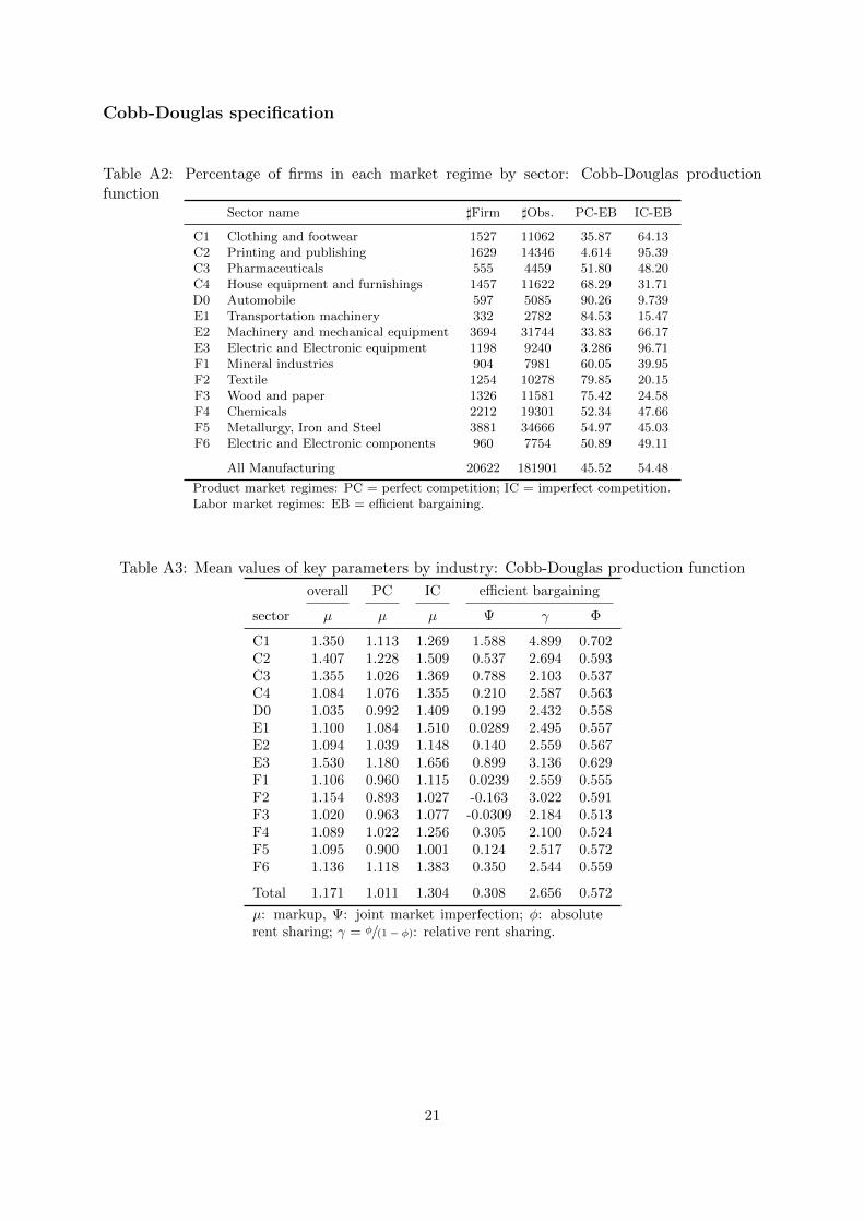
Cobb-Douglas specification

Table A2: Percentage of firms in each market regime by sector: Cobb-Douglas productionfunction

Sector name ]Firm ]Obs. PC-EB IC-EB

C1 Clothing and footwear 1527 11062 35.87 64.13C2 Printing and publishing 1629 14346 4.614 95.39C3 Pharmaceuticals 555 4459 51.80 48.20C4 House equipment and furnishings 1457 11622 68.29 31.71D0 Automobile 597 5085 90.26 9.739E1 Transportation machinery 332 2782 84.53 15.47E2 Machinery and mechanical equipment 3694 31744 33.83 66.17E3 Electric and Electronic equipment 1198 9240 3.286 96.71F1 Mineral industries 904 7981 60.05 39.95F2 Textile 1254 10278 79.85 20.15F3 Wood and paper 1326 11581 75.42 24.58F4 Chemicals 2212 19301 52.34 47.66F5 Metallurgy, Iron and Steel 3881 34666 54.97 45.03F6 Electric and Electronic components 960 7754 50.89 49.11

All Manufacturing 20622 181901 45.52 54.48

Product market regimes: PC = perfect competition; IC = imperfect competition.Labor market regimes: EB = efficient bargaining.

Table A3: Mean values of key parameters by industry: Cobb-Douglas production function

overall PC IC efficient bargaining

sector µ µ µ Ψ γ Φ

C1 1.350 1.113 1.269 1.588 4.899 0.702C2 1.407 1.228 1.509 0.537 2.694 0.593C3 1.355 1.026 1.369 0.788 2.103 0.537C4 1.084 1.076 1.355 0.210 2.587 0.563D0 1.035 0.992 1.409 0.199 2.432 0.558E1 1.100 1.084 1.510 0.0289 2.495 0.557E2 1.094 1.039 1.148 0.140 2.559 0.567E3 1.530 1.180 1.656 0.899 3.136 0.629F1 1.106 0.960 1.115 0.0239 2.559 0.555F2 1.154 0.893 1.027 -0.163 3.022 0.591F3 1.020 0.963 1.077 -0.0309 2.184 0.513F4 1.089 1.022 1.256 0.305 2.100 0.524F5 1.095 0.900 1.001 0.124 2.517 0.572F6 1.136 1.118 1.383 0.350 2.544 0.559

Total 1.171 1.011 1.304 0.308 2.656 0.572

µ: markup, Ψ: joint market imperfection; φ: absoluterent sharing; γ = φ/(1 − φ): relative rent sharing.

21

OLS estimation of trans-log specification

Table A4: Percentage of firms in each market regime by sector: OLS estimation of trans-logproduction function

Sector name ]Firm ]Obs. PC-PR PC-EB PC-MO IC-PR IC-EB IC-MO

C1 Clothing and footwear 1527 11062 4.216 1.702 1.349 1.597 90.72 0.419C2 Printing and publishing 1629 14346 3.303 1.179 1.196 9.140 84.05 1.137C3 Pharmaceuticals 555 4459 10.40 2.047 1.010 14.36 71.81 0.382C4 House equipment and furnishings 1457 11622 4.010 2.776 0.679 2.369 90.05 0.111D0 Automobile 597 5085 20.18 6.296 2.149 8.268 62.91 0.202E1 Transportation machinery 332 2782 27.67 1.155 7.271 14.88 47.65 1.369E2 Machinery and mechanical equipment 3694 31744 4.170 2.147 2.811 4.151 85.93 0.791E3 Electric and Electronic equipment 1198 9240 1.154 0.225 0.360 1.918 96.19 0.150F1 Mineral industries 904 7981 11.27 7.175 1.348 5.743 74.25 0.216F2 Textile 1254 10278 8.453 2.059 7.056 10.87 67.54 4.022F3 Wood and paper 1326 11581 18.43 4.006 8.796 11.87 55.90 1.001F4 Chemicals 2212 19301 11.93 7.567 2.643 7.224 69.79 0.848F5 Metallurgy, Iron and Steel 3881 34666 9.073 8.637 7.663 4.198 69.16 1.269F6 Electric and Electronic components 960 7754 3.574 2.984 0.759 2.006 90.49 0.185

All Manufacturing 20622 181901 8.221 4.343 3.856 5.987 76.62 0.971

Product market regimes: PC = perfect competition; IC = imperfect competition.Labor market regimes: PR = perfect comp.; EB = efficient bargaining; MO = monopsony.

Table A5: Mean values of key parameters by industry: OLS estimation of trans-log productionfunction

overall PC IC efficient bargaining monopsony

sector µ µ µ Ψ γ Φ Ψ β εLs

w

C1 1.235 0.953 1.290 0.678 2.903 0.625 -0.664 0.706 5.094C2 1.253 0.962 1.285 0.525 2.101 0.545 -0.321 0.795 5.064C3 1.212 0.955 1.281 0.757 1.753 0.503 -0.457 0.693 2.479C4 1.160 0.947 1.218 0.550 2.360 0.587 -0.295 0.771 4.323D0 1.101 0.958 1.188 0.470 2.053 0.547 -0.266 0.783 4.078E1 1.122 0.955 1.235 0.534 1.927 0.539 -0.374 0.731 3.330E2 1.150 0.947 1.193 0.444 2.062 0.556 -0.259 0.828 6.834E3 1.338 0.945 1.379 0.753 2.848 0.633 -0.332 0.759 3.909F1 1.124 0.950 1.213 0.471 1.780 0.501 -0.240 0.805 5.152F2 1.155 0.947 1.223 0.517 1.898 0.510 -0.287 0.812 5.704F3 1.087 0.955 1.168 0.485 1.580 0.487 -0.266 0.790 4.670F4 1.106 0.947 1.190 0.447 1.682 0.497 -0.289 0.787 4.670F5 1.114 0.944 1.191 0.421 1.709 0.504 -0.222 0.825 6.615F6 1.202 0.966 1.252 0.661 2.507 0.604 -0.359 0.749 4.134

Total 1.159 0.949 1.227 0.514 2.041 0.542 -0.275 0.806 5.786

µ: markup, Ψ: joint market imperfection; φ: absolute rent sharing; γ = φ/(1 − φ):relative rent sharing; εL

s

w : wage elasticity of the labor supply; β = εLs

w /(1 − εLs

w ):degree of monopsony power.

22