international energy agency building energy simulaltion ... · volume 1: cases e100–e200 j....

January 2002 Technical ReportNREL/TP-550-30152

International Energy Agency Building Energy Simulation Test andDiagnostic Method for Heating, Ventilating, and Air-Conditioning

Equipment Models (HVAC BESTEST)

Volume 1: Cases E100–E200

J. NeymarkJ. Neymark & Associates, Golden, Colorado

R. JudkoffNational Renewable Energy Laboratory, Golden, Colorado

National Renewable Energy Laboratory1617 Cole Boulevard

Golden, Colorado 80401-3393

http://www.nrel.gov/docs/fy02osti/30152CD.exe

NOTICE

This report was prepared as an account of work sponsored by an agency of the United States government.Neither the United States government nor any agency thereof, nor any of their employees, makes anywarranty, express or implied, or assumes any legal liability or responsibility for the accuracy, completeness,or usefulness of any information, apparatus, product, or process disclosed, or represents that its use wouldnot infringe privately owned rights. Reference herein to any specific commercial product, process, or serviceby trade name, trademark, manufacturer, or otherwise does not necessarily constitute or imply itsendorsement, recommendation, or favoring by the United States government or any agency thereof. Theviews and opinions of authors expressed herein do not necessarily state or reflect those of the United Statesgovernment or any agency thereof.

Available electronically at http://www.osti.gov/bridge

Available for a processing fee to U.S. Department of Energyand its contractors, in paper, from:

U.S. Department of EnergyOffice of Scientific and Technical InformationP.O. Box 62Oak Ridge, TN 37831-0062phone: 865.576.8401fax: 865.576.5728email: [email protected]

Available for sale to the public, in paper, from:U.S. Department of CommerceNational Technical Information Service5285 Port Royal RoadSpringfield, VA 22161phone: 800.553.6847fax: 703.605.6900email: [email protected] ordering: http://www.ntis.gov/ordering.htm

Printed on paper containing at least 50% wastepaper, including 20% postconsumer waste

http://www.osti.gov/bridge

http://www.ntis.gov/ordering.htm

iii

Acknowledgments

The work described in this report was a cooperative effort involving the members of the InternationalEnergy Agency (IEA) Model Evaluation and Improvement Experts Group. The group was composed ofexperts from the IEA Solar Heating and Cooling (SHC) Programme, Task 22, and was chaired byR. Judkoff of the National Renewable Energy Laboratory (NREL) on behalf of the U.S. Department ofEnergy (DOE). We gratefully acknowledge the contributions from the modelers and the authors ofsections on each of the computer programs used in this effort:

• Analytical Solution, HTAL: M. Duerig, A. Glass, and G. Zweifel; HochschuleTechnik+Architektur Luzern, Switzerland

• Analytical Solution, TUD: H.-T. Le and G. Knabe; Technische Universität Dresden, Germany

• CA-SIS V1: S. Hayez and J. Féburie; Electricité de France, France

• CLIM2000 V2.4: G. Guyon, J. Féburie, and R. Chareille of Electricité de France, France ; S.Moinard of Créteil University, France ; and J.-S. Bessonneau of Arob@s Technologies, France.

• DOE-2.1E ESTSC Version 088: J. Travesi; Centro de Investigaciones Energéticas,Medioambientales y Tecnologicas, Spain

• DOE-2.1E J.J. Hirsch Version 133: J. Neymark; J. Neymark & Associates, USA

• ENERGYPLUS Version 1.0.0.023: R. Henninger and M. Witte; GARD Analytics, USA

• PROMETHEUS: M. Behne; Klimasystemtechnik, Germany

• TRNSYS-TUD 14.2: H.-T. Le and G. Knabe; Technische Universität Dresden, Germany.

Additionally, D. Cawley and M. Houser of The Trane Company, USA, were very helpful with providingperformance data for, and answering questions about, unitary space cooling equipment.

Also, we appreciate the support and guidance of M. Holtz, operating agent for Task 22; and D. Crawley,DOE program manager for Task 22 and DOE representative to the IEA SHC Programme ExecutiveCommittee.

iv

Preface

Background and Introduction to the International Energy Agency

The International Energy Agency (IEA) was established in 1974 as an autonomous agency within theframework of the Organization for Economic Cooperation and Development (OECD) to carry out acomprehensive program of energy cooperation among its 24 member countries and the Commission ofthe European Communities.

An important part of the Agency’s program involves collaboration in the research, development, anddemonstration of new energy technologies to reduce excessive reliance on imported oil, increase long-term energy security, and reduce greenhouse gas emissions. The IEA’s R&D activities are headed by theCommittee on Energy Research and Technology (CERT) and supported by a small Secretariat staff,headquartered in Paris. In addition, three Working Parties are charged with monitoring the variouscollaborative energy agreements, identifying new areas for cooperation, and advising the CERT on policymatters.

Collaborative programs in the various energy technology areas are conducted under ImplementingAgreements, which are signed by contracting parties (government agencies or entities designated bythem). There are currently 40 Implementing Agreements covering fossil fuel technologies, renewableenergy technologies, efficient energy end-use technologies, nuclear fusion science and technology, andenergy technology information centers.

Solar Heating and Cooling Program

The Solar Heating and Cooling Program was one of the first IEA Implementing Agreements to beestablished. Since 1977, its 21 members have been collaborating to advance active solar, passive solar, andphotovoltaic technologies and their application in buildings.

The members are:

Australia France Norway

Austria Germany Portugal

Belgium Italy Spain

Canada Japan Sweden

Denmark Mexico Switzerland

European Commission Netherlands United Kingdom

Finland New Zealand United States

A total of 26 Tasks have been initiated, 17 of which have been completed. Each Task is managed by anOperating Agent from one of the participating countries. Overall control of the program rests with anExecutive Committee comprised of one representative from each contracting party to the ImplementingAgreement. In addition, a number of special ad hoc activities—working groups, conferences, andworkshops—have been organized.

v

The Tasks of the IEA Solar Heating and Cooling Programme, both completed and current, are as follows:

Completed Tasks:Task 1 Investigation of the Performance of Solar Heating and Cooling Systems

Task 2 Coordination of Solar Heating and Cooling R&D

Task 3 Performance Testing of Solar Collectors

Task 4 Development of an Insolation Handbook and Instrument Package

Task 5 Use of Existing Meteorological Information for Solar Energy Application

Task 6 Performance of Solar Systems Using Evacuated Collectors

Task 7 Central Solar Heating Plants with Seasonal Storage

Task 8 Passive and Hybrid Solar Low Energy Buildings

Task 9 Solar Radiation and Pyranometry Studies

Task 10 Solar Materials R&D

Task 11 Passive and Hybrid Solar Commercial Buildings

Task 12 Building Energy Analysis and Design Tools for Solar Applications

Task 13 Advanced Solar Low Energy Buildings

Task 14 Advanced Active Solar Energy Systems

Task 16 Photovoltaics in Buildings

Task 17 Measuring and Modeling Spectral Radiation

Task 18 Advanced Glazing and Associated Materials for Solar and Building Applications

Task 19 Solar Air Systems

Task 20 Solar Energy in Building Renovation

Task 21 Daylight in Buildings

Current Tasks and Working Groups:Task 22 Building Energy Analysis Tools

Task 23 Optimization of Solar Energy Use in Large Buildings

Task 24 Solar Procurement

Task 25 Solar Assisted Cooling Systems for Air Conditioning of Buildings

Task 26 Solar Combisystems Working Group Materials in Solar Thermal Collectors

Task 27 Performance Assessment of Solar Building Envelope Components

Task 28 Solar Sustainable Housing

Task 29 Solar Crop Drying

Task 30 Solar Cities

vi

Task 22: Building Energy Analysis Tools

Goal and Objectives of the TaskThe overall goal of Task 22 is to establish a sound technical basis for analyzing solar, low-energybuildings with available and emerging building energy analysis tools. This goal will be pursued byaccomplishing the following objectives:

• Develop methods to assess the accuracy of available building energy analysis tools in predictingthe performance of widely used solar and low-energy concepts;

• Collect and document engineering models of widely used solar and low-energy concepts for usein the next generation building energy analysis tools;

• Assess and document the impact (value) of improved building analysis tools in analyzing solar,low-energy buildings; and

• Widely disseminate research results and analysis tools to software developers, industryassociations, and government agencies.

Scope of the TaskThis Task will investigate the availability and accuracy of building energy analysis tools and engineeringmodels to evaluate the performance of solar and low-energy buildings. The scope of the Task is limitedto whole building energy analysis tools, including emerging modular type tools, and to widely used solarand low-energy design concepts. Tool evaluation activities will include analytical, comparative, andempirical methods, with emphasis given to blind empirical validation using measured data from testrooms of full-scale buildings. Documentation of engineering models will use existing standard reportingformats and procedures. The impact of improved building energy analysis will be assessed from abuilding owner perspective.

The audience for the results of the Task is building energy analysis tool developers. However, tool users,such as architects, engineers, energy consultants, product manufacturers, and building owners andmanagers, are the ultimate beneficiaries of the research, and will be informed through targeted reportsand articles.

MeansIn order to accomplish the stated goal and objectives, the Participants will carry out research in theframework of two Subtasks:

Subtask A: Tool Evaluation

Subtask B: Model Documentation

ParticipantsThe participants in the Task are: Finland, France, Germany, Spain, Sweden, Switzerland, UnitedKingdom, and United States. The United States serves as Operating Agent for this Task, with Michael J.Holtz of Architectural Energy Corporation providing Operating Agent services on behalf of the U.S.Department of Energy.

This report documents work carried out under Subtask A.2, Comparative and Analytical VerificationStudies.

vii

Table of Contents

Acknowledgements ..................................................................................................................... iii

Preface ..................................................................................................................... iv

Electronic Media Contents .......................................................................................................................x

Executive Summary ..................................................................................................................... xi

Background .....................................................................................................................xx

References for Front Matter ..................................................................................................................xxx

1.0 Part I: Heating, Ventilating, and Air-Conditioning (HVAC) BESTEST User’s Manual—Procedure and Specification ........................................................................................................... I-1

1.1 General Description of Test Cases ........................................................................................ I-1

1.2 Performing the Tests.............................................................................................................. I-4

1.2.1 Input Requirements ...................................................................................................... I-4

1.2.2 Modeling Rules ............................................................................................................ I-4

1.2.3 Output Requirements.................................................................................................... I-5

1.2.4 Comparing Your Output to the Analytical Solution and Example SimulationResults .................................................................................................................... I-6

1.3 Specific Input Information..................................................................................................... I-7

1.3.1 Weather Data................................................................................................................ I-7

1.3.2 Case E100 Base Case Building and Mechanical System............................................. I-9

1.3.2.1 Building Zone Description......................................................................... I-9

1.3.2.1.1 Building Geometry .......................................................................... I-9

1.3.2.1.2 Building Envelope Thermal Properties ........................................... I-9

1.3.2.1.3 Weather Data ................................................................................. I-12

1.3.2.1.4 Infiltration...................................................................................... I-12

1.3.2.1.5 Internal Heat Gains ........................................................................ I-12

1.3.2.1.6 Opaque Surface Radiative Properties ............................................ I-12

1.3.2.1.7 Exterior Combined Radiative and Convective SurfaceCoefficients.................................................................................... I-12

1.3.2.1.8 Interior Combined Radiative and Convective SurfaceCoefficients.................................................................................... I-12

viii

1.3.2.2 Mechanical System .................................................................................. I-13

1.3.2.2.1 General Information....................................................................... I-14

1.3.2.2.2 Thermostat Control Strategy ......................................................... I-14

1.3.2.2.3 Full Load Cooling System Performance Data ............................... I-15

1.3.2.2.4 Part Load Operation....................................................................... I-24

1.3.2.2.5 Evaporator Coil.............................................................................. I-25

1.3.2.2.6 Fans................................................................................................ I-27

1.3.3 Additional Dry Coil Test Cases ................................................................................. I-28

1.3.3.1 Case E110: Reduced Outdoor Dry-bulb Temperature ............................. I-28

1.3.3.2 Case E120: Increased Thermostat Setpoint ............................................. I-28

1.3.3.3 Case E130: Low Part Load Ratio............................................................. I-28

1.3.3.4 Case E 140: Reduced ODB at Low PLR.................................................. I-28

1.3.4 Humid Zone Test Cases.............................................................................................. I-29

1.3.4.1 Case E150: Latent Load at High Sensible Heat Ratio ............................. I-29

1.3.4.2 Case E160: Increased Thermostat Set Point at High SHR....................... I-29

1.3.4.3 Case E165: Variation of Thermostat and ODB at High SHR.................. I-29

1.3.4.4 Case E170: Reduced Sensible Load......................................................... I-30

1.3.4.5 Case E180: Increased Latent Load........................................................... I-30

1.3.4.6 Case E185: Increased ODB at Low SHR................................................. I-30

1.3.4.7 Case E190: Low Part Load Ratio at Low SHR........................................ I-30

1.3.4.8 Case E195: Increased ODB at Low SHR and Low PLR ......................... I-30

1.3.4.9 Case E200: Full Load Test at ARI Conditions ........................................ I-31

Appendix A – Weather Data Format Description ........................................................................ I-32

A.1 Typical Meteorological Year (TMY) Format ............................................................ I-32

A.2 Typical Meteorological Year 2 ((TMY2) Data and Format....................................... I-39

Appendix B – COP Degradation Factor (CDF) as a Function of Part Load Ratio (PLR)............ I-47

Appendix C – Cooling Coil Bypass Factor .................................................................................. I-48

Appendix D – Indoor Fan Data Equivalence................................................................................ I-53

Appendix E – Output Spreadsheet Instructions............................................................................ I-55

Appendix F – Diagnosing the Results Using the Flow Diagrams ................................................ I-57

Appendix G – Abbreviations and Acronyms................................................................................ I-60

Appendix H – Glossary ................................................................................................................ I-61

References for Part I .................................................................................................................. I-64

ix

2.0 Part II: Production of Analytical Solution Results ...........................................................................II-1

2.1 Introduction ...................................................................................................................II-1

2.2 Comparison of Analytical Solution Results and Resolution of Disagreements ...................II-2

2.3 Documentation of the Solutions ...........................................................................................II-6

2.3.1 Analytical Solutions by Technische Universität Dresden (TUD) ...............................II-7

2.3.2 Analytical Solutions by Hochschule Technik + Architektur Luzern (HTAL)..........II-37

2.4 Analytical Solution Results Tables ....................................................................................II-58

2.5 Referencesfor Part II ..........................................................................................................II-61

2.6 Abbreviations and Acronyms for Part II ............................................................................II-61

3.0 Part III: Production of Simulation Results .....................................................................................III-1

3.1 Introduction ..................................................................................................................III-1

3.2 Selection of Simulation Programs and Modeling Rules for Simulations............................III-1

3.3 Improvements to the Test Specification as a Result of the Field Trials..............................III-2

3.4 Examples of Error Trapping with HVAC BESTEST Diagnostics......................................III-3

3.5 Interpretation of Results ....................................................................................................III-21

3.6 Conclusions and Recommendations..................................................................................III-25

3.7 Acronyms for Part III.........................................................................................................III-30

3.8 References for Part III .......................................................................................................III-31

3.9 Appendix III: Simulation Modeler Reports.......................................................................III-32

Appendix III-A: DOE-2.1E JJHirsch version 133, NREL ................................................III-33

Appendix III-B: TRNSYS-TUD, TUD..............................................................................III-52

Appendix III-C: CLIM2000 V2.1.6 & V2.4, EDF ............................................................III-86

Appendix III-D: CA-SIS V1, EDF ..................................................................................III-105

Appendix III-E: DOE-2.1E ESTSC version 088, CIEMAT............................................III-117

Appendix III-F: PROMETHEUS, KST...........................................................................III-128

Appendix III-G: EnergyPlus version 1.00.023, GARD Analytics...................................III-130

4.0 Part IV: Simulation Field Trial Results .......................................................................................... IV-1

x

Electronic Media Contents

Files apply as they are called out in the test procedure.

README.DOC: Electronic media contents

HVBT294.TM2: TMY2 weather data with constant ODB = 29.4°C

HVBT294.TMY: TMY weather data with constant ODB = 29.4°C







HVBTOUT.XLS: Raw output data spreadsheet used by the IEA participants

PERFMAP.XLS: Performance data (Tables 1-6a through 1-6f)

RESULTS.DOC: Documentation for navigating RESULTS.XLS

RESULTS.XLS: Results spreadsheet to assist users with plotting their results versus analyticalsolution results and other simulation results

\INPDECKS subdirectory (IEA SHC Task 22 participant simulation input decks)

\DOE2-CIEMAT

\DOE2-NREL

\ENERGYPLUS

\TRNSYS-TUD

Note: Final input decks were not submitted for CASIS, CLIM2000, or PROMETHEUS.

xi

Executive Summary

Objectives

This report describes the Building Energy Simulation Test for Heating, Ventilating, and Air-Conditioning Equipment Models (HVAC BESTEST) project conducted by the Tool Evaluation andImprovement International Energy Agency (IEA) Experts Group. The group was composed of expertsfrom the Solar Heating and Cooling (SHC) Programme, Task 22, Subtask A. The current test cases,E100–E200, represent the beginning of work on mechanical equipment test cases; additional cases thatwould expand the current test suite have been proposed for future development.

The objective of the tool evaluation subtask has been to develop practical procedures and data for anoverall IEA validation methodology that the National Renewable Energy Laboratory (NREL) has beendeveloping since 1981 (Judkoff et al. 1983; Judkoff 1988), with refinements contributed byrepresentatives of the United Kingdom (Lomas 1991; Bloomfield 1989) and the American Society ofHeating, Refrigerating, and Air-Conditioning Engineers (American National Standards Institute[ANSI]/ASHRAE Standard 140-2001). The methodology combines empirical validation, analyticalverification, and comparative analysis techniques and is discussed in detail in the following Backgroundsection. This report documents an analytical verification and comparative diagnostic procedure fortesting the ability of whole-building simulation programs to model the performance of unitary spacecooling equipment that is typically modeled using manufacturer design data presented in the form ofempirically derived performance maps. The report also includes results from analytical solutions as wellas from simulation programs that were used in field trials of the test procedure. Other projects conductedby Task 22, Subtask A and reported elsewhere, included work on empirical validation (Guyon andMoinard 1999; Palomo and Guyon 1999; Travesi et al 2001) and analytical verification (Tuomaala 1999;San Isidro 2000). In addition, Task 22, Subtask B has produced a report on the application of the NeutralModel Format in building energy simulation programs (Bring et al 1999).

In this project the BESTEST method, originally developed for use with envelope models in IEA SHCTask 12 (Judkoff and Neymark 1995a), was extended for testing mechanical system simulation modelsand diagnosing sources of predictive disagreements. Cases E100–E200, described in this report, apply tounitary space cooling equipment. Testing of additional cases, which cover other aspects of HVACequipment modeling, is planned for the future. Field trials of HVAC BESTEST were conducted with anumber of detailed state-of-the-art simulation programs from the United States and Europe including: CA-SIS, CLIM2000, DOE-2, ENERGYPLUS, PROMETHEUS, and TRNSYS. The process was iterativein that executing the simulations led to the refining of HVAC BESTEST, and the results of the tests ledto improving and debugging the programs.

HVAC BESTEST consists of a series of steady-state tests using a carefully specified mechanical coolingsystem applied to a highly simplified near-adiabatic building envelope. Because the mechanicalequipment load is driven by sensible and latent internal gains, the sensitivity of the simulation programsto a number of equipment performance parameters is explored. Output values for the cases such ascompressor and fan electricity consumption, cooling coil sensible and latent loads, coefficient ofperformance (COP), zone temperature, and zone humidity ratio are compared and used in conjunctionwith a formal diagnostic method to determine the algorithms responsible for predictive differences. Inthese steady-state cases, the following parameters are varied: sensible internal gains, latent internal gains,zone thermostat set point (entering dry-bulb temperature), and outdoor dry-bulb temperature (ODB). Toobtain steady-state ODB, ambient dry-bulb temperatures were held constant in the weather data filesprovided with the test cases. Parametric variations isolate the effects of the parameters singly and in

xii

various combinations, as well as the influence of: part-loading of equipment, varying sensible heat ratio,“dry” coil (no latent load) versus “wet” coil (with dehumidification) operation, and operation at typicalAir-Conditioning and Refrigeration Institute (ARI) rating conditions. In this way the models are tested invarious domains of the performance map.

As a BESTEST user, if you have not already tested your software’s ability to model envelope loads, westrongly recommend that you run the envelope-load tests in addition to HVAC BESTEST. A set ofenvelope loads tests is included in ASHRAE Standard 140 (ANSI/ASHRAE 2001); the Standard 140 testcases are based on IEA BESTEST (Judkoff and Neymark 1995a). Another set of envelope-load testcases, which were designed to test simplified tools such as those currently used for home energy ratingsystems, is included in HERS BESTEST (Judkoff and Neymark 1995b; Judkoff and Neymark 1997).HERS BESTEST has a more realistic base building than IEA BESTEST; however, its ability to diagnosesources of differences among results is not as detailed (Neymark and Judkoff 1997).

Significance of the Analytical Solution Results

A methodological difference between this work and the envelope BESTEST work of Task 12 is that thiswork includes analytical solutions. In general, it is difficult to develop worthwhile test cases that can besolved analytically, but such solutions are extremely useful when possible. The analytical solutionsrepresent a “mathematical truth standard” for cases E100–E200. Given the underlying physicalassumptions in the case definitions, there is a mathematically provable and deterministic solution foreach case. In this context, the underlying physical assumptions about the mechanical equipment (asdefined in cases E100–E200) are representative of typical manufacturer data. These data, with whichmany whole-building simulation programs are designed to work, are normally used by building designpractitioners. It is important to understand the difference between a mathematical truth standard and an“absolute truth standard.” In the former, we accept the given underlying physical assumptions whilerecognizing that these assumptions represent a simplification of physical reality. The ultimate or absolutevalidation standard would be a comparison of simulation results with a perfectly performed empiricalexperiment, the inputs for which are perfectly specified to the simulationists. In reality an experiment isperformed and the experimental object is specified within some acceptable band of uncertainty. Suchexperiments are possible but fairly expensive. In the section on future work, we recommend developing aset of empirical validation experiments.

Two of the participating organizations independently developed analytical solutions that were submittedto a third party for review. Comparison of the results indicated some disagreements, which were thenresolved by allowing the solvers to review the comments from the third party reviewers, and to alsoreview and critique each other’s solution techniques. As a result of this process, both solvers madelogical and non-arbitrary changes to their solutions such that their final results are mostly well within a<1% range of disagreement. Remaining minor differences in the analytical solutions are due in part to thedifficulty of completely describing boundary conditions. In this case the boundary conditions are acompromise between full reality and some simplification of the real physical system that is analyticallysolvable. Therefore, the analytical solutions have some element of interpretation of the exact nature ofthe boundary conditions, which causes minor disagreement in the results. For example, in the modelingof the controller, one group derived an analytical solution for an “ideal” controller, while another groupdeveloped a numerical solution for a “realistic” controller. Each solution yields slightly different results,but both are correct in the context of this exercise. Although this may be less than perfect from amathematician’s viewpoint, it is quite acceptable from an engineering perspective.

The remaining minor disagreements among analytical solutions are small enough to allow identificationof bugs in the software that would not otherwise be apparent from comparing software only to othersoftware. Therefore, having cases that are analytically solvable when possible improves the diagnostic

xiii

capabilities of the test procedure. As test cases become more complex, it is rarely possible to solve themanalytically.

Field Trial Results

Disagreement among Simulation ProgramsAfter correcting software errors using HVAC BESTEST diagnostics, the mean results of COP and totalenergy consumption for the simulation programs are on average within <1% of the analytical solutionresults, with average variations of up to 2% for the low part load ratio (PLR) dry-coil cases (E130 andE140). Ranges of disagreement are further summarized in Table ES-1for predictions of various outputs,disaggregated for dry-coil performance (no dehumidification) and for wet-coil performance(dehumidification moisture condensing on the coil). This range of disagreement for each case is based onthe difference between each simulation result versus the mean of the analytical solution results, dividedby the mean of the analytical solution results. This summary excludes results for one of the participantswho suspected an error(s) in their software, but were not able to correct their results or complete theproject.

Table ES-1. Ranges of Disagreement among Simulation Results

CasesDry Coil(E100-E140)

Wet Coil(E150-E200)

COP and Total ElectricConsumption

0% - 6%a 0% - 3%a

Zone Humidity Ratio 0% - 11%a 0% - 7%a

Zone Temperature 0.0°C - 0.7°C (0.1°C)b

0.0°C - 0.5°C (0.0°C – 0.1°C)b

a Percentage disagreement for each case is based on the difference between each simulation result (excluding one simulation participant that could not finish the project) versus the mean of the analytical solution results, divided by the mean of the analytical solution results.b Excludes results for TRNSYS-TUD with realistic controller.

In Table ES-1, the higher level of disagreement in the dry-coil cases occurs for the case with lowest PLR;further discussion of specific disagreements is included in Part III (e.g., Sections 3.4 and 3.5). Thedisagreement in zone temperature results is primarily from one simulation that applies a realisticcontroller on a short time step (36 seconds); all other simulation results apply ideal control.

Based on results after “HVAC BESTESTing,” the programs appear reliable for performance-mapmodeling of space cooling equipment when the equipment is operating close to design conditions. In thefuture, HVAC BESTEST cases will explore modeling at “off-design” conditions and the effects of usingmore realistic control schemes.

Bugs Found in Simulation ProgramsThe results generated with the analytical solution techniques and the simulation programs are intended tobe useful for evaluating other detailed or simplified building energy prediction tools. The group’scollective experience has shown that when a program exhibits major disagreement with the analyticalsolution results given in Part II, the underlying cause is usually a bug, a faulty algorithm, or adocumentation problem. During the field trials, the HVAC BESTEST diagnostic methodology was

xiv

successful at exposing such problems in every one of the simulation programs tested. The most notableexamples are listed below; a full listing appears in the conclusions section of Part III.

• Isolation and correction of a coding error related to calculation of minimum supply airtemperature in the DOE-2.1E mechanical system model “RESYS2”; this affected base caseefficiency estimates by 36%. (Until recently, DOE-2 was the main building energy analysisprogram sponsored by the U.S. Department of Energy [DOE]; many of its algorithms are beingincorporated into DOE's next-generation simulation software, ENERGYPLUS.)

• Isolation and correction of a problem associated with using single precision variables, rather thandouble precision variables, in an algorithm associated with modeling a realistic controller inTRNSYS-TUD; this affected compressor power estimates by 14% at medium PLR, and by 45%at low PLR. (TRNSYS is the main program for active solar systems analysis in the U.S.;TRNSYS-TUD is a version with custom algorithms developed by Technische UniversitätDresden, Germany.)

• Isolation of a missing algorithm to account for degradation of COP with decreasing PLR inCLIM2000 and in PROMETHEUS, and later inclusion of this algorithm in CLIM2000; thisaffected compressor power estimates by up to 20% at low PLR. (CLIM2000, which is primarilydedicated to research and development studies, is the most detailed of the building energyanalysis programs sponsored by the French national electric utility Electricité de France;PROMETHEUS is a detailed hourly simulation program sponsored by the architecturalengineering firm Klimasystemtechnik, Germany.)

• Isolation and correction of problems in CA-SIS associated with neglecting to include the fan heatwith the coil load. Neglecting the fan heat on coil load caused up to 4% underestimation of totalenergy consumption. (CA-SIS, which is based on TRNSYS, was developed by Electricité deFrance for typical energy analysis studies.)

• Isolation and correction of a coding error in ENERGYPLUS that excluded correction for runtime during cycling operation from reported coil loads. This caused reported coil loads to beoverestimated by a factor of up to 25 for cases with lowest PLR; there was negligible effect onenergy consumption and COP from this error. (ENERGYPLUS has recently been released byDOE as the building energy simulation program that will be supported by DOE.)

• Isolation of problems in CA-SIS, DOE-2.1E and ENERGYPLUS (which were corrected in CA-SIS and ENERGYPLUS) associated with neglecting to account for the effect of degradation ofCOP (increased run time) with decreasing PLR on the indoor and outdoor fan energyconsumptions. Neglecting the PLR effect on fan run time caused a 2% underestimation of totalenergy consumption at mid-range PLRs.

Additionally, Electricité de France software developers used this project to check on modelimprovements to CLIM2000 begun before this project began, and completed during the beginning of theproject. They demonstrated up to a 50% improvement in COP predictions over results of their previousversion.

Conclusions

An advantage of BESTEST is that a program is examined over a broad range of parametric interactionsbased on a variety of output types, minimizing the possibility for concealment of problems bycompensating errors. Performance of the tests resulted in quality improvements to all of the buildingenergy simulation programs used in this study. Many of the errors found during the project stemmedfrom incorrect code implementation. Some of these bugs may well have been present for many years. The

xv

fact that they have just now been uncovered shows the power of BESTEST and also suggests theimportance of continuing to develop formalized validation methods.

Checking a building energy simulation program with HVAC BESTEST requires about one person-weekfor an experienced user. Because the simulation programs have taken many years to produce, HVACBESTEST provides a very cost-effective way of testing them. As we continue to develop new test cases,we will adhere to the principle of parsimony so that the entire suite of BESTEST cases may beimplemented by users within a reasonable time span.

Architects, engineers, program developers, and researchers can use the HVAC BESTEST method in anumber of different ways, such as:

• To compare output from building energy simulation programs to a set of analytical solutions thatconstitute a reliable set of theoretical results given the underlying physical assumptions in thecase definitions

• To compare several building energy simulation programs to determine the degree ofdisagreement among them

• To diagnose the algorithmic sources of prediction differences among several building energysimulation programs

• To compare predictions from other building energy programs to the analytical solutions andsimulation results in this report

• To check a program against a previous version of itself after internal code modifications toensure that only the intended changes actually resulted

• To check a program against itself after a single algorithmic change to understand the sensitivityamong algorithms.

In general, the current generation of programs appears reliable for performance-map modeling of spacecooling equipment when the equipment is operating close to design conditions. However, the currentcases check extrapolation only to a limited extent. Additional cases have been defined for future work tofurther explore the issue of modeling equipment performance at off-design conditions, which are nottypically included within the performance data provided in manufacturer catalogs. As buildings becomemore energy efficient, either through conservation or via the integration of solar technology, the relativeimportance of equipment operation at off-design conditions increases. The tendency among somepractitioners to oversize equipment, as well as the importance of simulation for designing equipmentretrofits and upgrades, also emphasizes the importance of accurate off-design equipment modeling. Forthe state of the art in annual simulation of mechanical equipment to improve, manufacturers need toeither readily provide expanded data sets on the performance of their equipment or improve existingequipment selection software to facilitate the generation of such data sets.

Future Work: Recommended Additional Cases

The previous IEA BESTEST envelope test cases (Judkoff and Neymark 1995a) have been code-languageadapted and formally approved by ANSI and ASHRAE as a Standard Method of Test, ANSI/ASHRAEStandard 140 (ANSI/ASHRAE Standard 140-2001). The BESTEST procedures are also being used asteaching tools for simulation courses at universities in the United States and Europe.

The addition of mechanical equipment tests to the existing envelope tests gives building energy softwaredevelopers and users an expanded ability to test a program for reasonableness of results and to determineif a program is appropriate for a particular application. Cases E100–E200 emphasize the testing of aprogram’s modeling capabilities with respect to the building’s mechanical equipment on the working-

xvi

fluid side of the coil. These cases represent just the beginning of possible work on validation ofmechanical equipment models. In the course of this work it became apparent, based on comments fromthe participants and observations of the test specification authors, that some additional test cases wouldbe useful for improved error trapping and diagnostics with HVAC BESTEST. In future work, thefollowing extensions to the test suite should be considered. (A more complete listing is included in PartIII, Section 3.5.1.)

The following cases have been defined for an extension of Task 22 (Neymark and Judkoff 2001). Thesecases will not be possible to solve analytically, but will be developed as comparative test cases. They aredynamic test cases that utilize unrevised dynamic annual site weather data. They also help to scale thesignificance of disagreements that are less obvious with steady-state test cases. The cases test the abilityto model:

• Quasi-steady-state performance using dynamic boundary conditions (dynamic internal gainsloading and dynamic weather data)

• Latent loading from infiltration

• Outside air mixing

• Periods of operation away from typical design conditions

• Thermostat setup (dynamic operating schedule)

• Undersized system performance

• Economizer with a variety of control schemes

• Variation of PLR (using dynamic weather data)

• Outdoor dry-bulb temperature and entering dry-bulb temperature performance sensitivities (usingdynamic loading and weather data)

Additional cases and improvements that are also being considered for development as part of the Task 22extension are:

• Various control schemes including minimum on/off, hysteresis, and proportional controls

• Variation of part load performance based on more detailed data

• Variable air volume fan performance and control

• Heating equipment such as furnaces and heat pumps

• Radiant heating and cooling systems

• Multizone envelope heat transfer

• Update of simulation reference results for IEA (envelope) BESTEST and HERS BESTEST caseswith floor slab and below-grade wall ground-coupled heat transfer.

Longer-term work would include developing test cases for:

• Thermal storage equipment

• Air-to-air heat exchanger

• More complex systems associated with larger buildings, such as:

o Large chillerso Chilled water loops

xvii

o Cooling towers and related circulation loopso More complex air handling systemso Other “plant” equipment

• Equivalent inputs for highly detailed unitary system primary loop component models of, forexample, compressors, condensers, evaporators, and expansion valves.

More envelope modeling test cases could be included such as:

• Improved ground coupling cases

• Expanded infiltration tests (e.g., testing algorithms that vary infiltration with wind speed)

• Vary radiant fraction of heat sources

• Moisture adsorption/desorption.

ASHRAE is also conducting related work to develop tests related to the airside of the mechanicalequipment in commercial buildings (Yuill 2001).

Closing Remarks

The previous IEA BESTEST procedure (Judkoff and Neymark 1995a), developed in conjunction withIEA SHC Task 12, has been code-language-adapted and approved by ANSI and ASHRAE as a StandardMethod of Test for evaluating building energy analysis computer programs (ANSI/ASHRAE Standard140-2001). This method primarily tests envelope-modeling capabilities. We anticipate that after codelanguage adaptation, HVAC BESTEST will be added to that Standard Method of Test. In the UnitedStates, the National Association of State Energy Officials (NASEO) Residential Energy ServicesNetwork (RESNET) has also adopted HERS BESTEST (Judkoff and Neymark 1995b) as the basis forcertifying software to be used for Home Energy Rating Systems under the association’s nationalguidelines. The BESTEST procedures are also being used as teaching tools for simulation courses atuniversities in the United States and Europe. We hope that as the procedures become better known,developers will automatically run the tests as part of their normal in-house quality control efforts. Thelarge number of requests (more than 800) that we have received for the envelope BESTEST reportsindicates that this is beginning to happen. Developers should also include the test input and output fileswith their respective software packages to be used as part of the standard benchmarking process.

Clearly, there is a need for further development of simulation models, combined with a substantialprogram of testing and validation. Such an effort should contain all the elements of an overall validationmethodology (see the following Background section), including:

• Analytical verification

• Comparative testing and diagnostics

• Empirical validation.

Future work should therefore encompass:

• Continued production of a standard set of analytical verification tests

• Development of a sequentially ordered series of high-quality data sets for empirical validation

• Development of a set of diagnostic comparative tests that emphasize the modeling issuesimportant in large commercial buildings, such as zoning and more tests for heating, ventilation,and air-conditioning systems.

xviii

Continued support of model development and validation activities is essential because occupiedbuildings are not amenable to classical controlled, repeatable experiments. The energy, comfort, andlighting performance of buildings depends on the interactions among a large number of energy transfermechanisms, components, and systems. Simulation is the only practical way to bring a systemsintegration problem of this magnitude within the grasp of designers. Greatly reducing the energy intensityof buildings through better design is possible with the use of such simulation tools. However, buildingenergy simulation programs will not come into widespread use unless the design and engineeringcommunities have confidence in these programs. Confidence can best be encouraged by a rigorousdevelopment and validation effort, combined with friendly user interfaces to minimize human error andeffort.

Finally, the authors wish to acknowledge that the expertise available through IEA and the dedication ofthe participants were essential to the success of this project. For example, when the test cases weredeveloped, they were originally intended as comparative tests, so that there would be simulation resultsbut not analytical solution results. However, after initial development of the steady-state tests, it becameapparent to us that analytical solutions would be possible. The participating countries provided theexpertise to derive two independent sets of analytical solutions and a third party to examine the results ofthe two original solvers. Also, over the 3-year field trial effort, there were several revisions to the HVACBESTEST specifications and subsequent re-executions of the computer simulations. This iterativeprocess led to the refining of HVAC BESTEST, and the results of the tests led to improving anddebugging of the programs. The process underscores the leveraging of resources for the IEA countriesparticipating in this project. Such extensive field trials, and resulting enhancements to the tests, weremuch more cost effective with the participation of the IEA SHC Task 22 experts.

Final Report Structure

This report is divided into four parts. Part I is a user's manual that furnishes instructions on how to applythe HVAC BESTEST procedure. Part II describes what two of the working group participants did todevelop analytical solutions independently, including a third-party comparison. After the third-partycomparison and comments, there was intense follow-up comparison and discussion among the initialsolvers to revise the analytical solutions so a high level of agreement was achieved. The last section ofPart II also includes a tabulation of the analytical solution results by each solver along with disagreementstatistics. Part II will be useful to those wanting to understand the physical theories and assumptionsunderlying the test cases. However, with the exception of the last section, which includes the finalanalytical results tables, it is not necessary to read Part II to implement the test procedure.

Part III describes what the working group members did to field-test HVAC BESTEST and produce a setof results using several state-of-the-art, detailed whole-building energy simulation programs with timesteps of 1 hour or less. This includes a summary compilation of significant bugs found in all thesimulation programs as a result of their testing in the field trials. Part III is helpful for understanding howother simulationists implemented the test procedure and applied the diagnostic logic. However, it is notnecessary to read Part III to implement the test procedure.

Part IV presents both the analytical solution and simulation program results in tables and graphs alongwith disagreement statistics comparing the simulation programs to each other and to the analyticalsolutions. These data can be used to compare results from other programs to Part IV results, and toobserve the range of disagreement among the simulation programs used for the field trials versus theanalytical solutions.

xix

The report includes electronic media that contains the weather data and all the analytical solution andsimulation program results in a common spreadsheet format, along with participants’ simulation inputdata.

Additionally, we have included with the front matter the following Background section that includes anoverview of validation methodology and a summary of previous NREL, IEA-related, and other validationwork related to software that analyzes energy use in buildings.

xx

Background

This section summarizes some of the work that preceded this BESTEST effort and describes the overallmethodological and historical context for BESTEST.

The increasing power and attractive pricing of personal computers has engendered a proliferation ofbuilding energy analysis software. An on-line directory sponsored by DOE (Building Energy ToolsDirectory 2001) lists more than 200 building energy software tools that have thousands of usersworldwide. Such tools utilize a number of different approaches to calculating building energy usage(Gough 1999). There is little if any objective quality control of much of this software. An earlyevaluation of a number of design tools conducted in IEA’s SHC Programme Task 8 showed largeunexplained predictive differences between these tools, even when run by experts (Rittelmann andAhmed 1985). More recent work to develop software testing and evaluation procedures indicates that thecauses of predictive differences can be isolated, and that bugs that may be causing anomalous differencescan be found and fixed, resulting in program improvements. However, even with improved capabilitiesfor testing and evaluating software, predictive differences remain (Judkoff and Neymark 1995a, 1995b).

Users of building energy simulation tools must have confidence in their utility and accuracy because theuse of such tools offers a great potential for energy savings and comfort improvements. Validation andtesting is a necessary part of any software development process, and is intended to stimulate theconfidence of the user. In recognition of the benefits of testing and validation, an effort was begun underIEA SHC Task 8, and continued in SHC Task 12 Subtask B and Buildings and Community Systems (BCS)Annex 21 Subtask C, to develop a quantitative procedure for evaluating and diagnosing building energysoftware (Judkoff et al. 1988; Bloomfield 1989). The procedure that resulted from that effort is called theBuilding Energy Simulation Test (BESTEST) and Diagnostic Method (Judkoff and Neymark 1995a). Thisinitial version of BESTEST focused on evaluating a simulation program’s ability to model buildingenvelope heat transfer, and to model basic thermostat controls and mechanical ventilation. As part of SHCTask 22, the BESTEST work was expanded to include more evaluation of heating, ventilating and air-conditioning (HVAC) equipment models. This new procedure, which is the subject of this report, is calledHVAC BESTEST.

Before the inception of IEA SHC Task 8, NREL (then the Solar Energy Research Institute) had begunworking on a comprehensive validation methodology for building energy simulation programs (Judkoffet al. 1983). This effort was precipitated by two comparative studies that showed considerable disagreementbetween four simulation programs—DOE-2, BLAST, DEROB, and SUNCAT—when given equivalentinput for a simple direct-gain solar building with a high and low heat capacitance parametric option(Judkoff, Wortman, and Christensen 1980; Judkoff, Wortman, and O’Doherty 1981). These studies clearlyindicated the need for a validation effort based on a sound methodological approach.

Validation Methodology

A typical building energy simulation program contains hundreds of variables and parameters. The numberof possible cases that can be simulated by varying each of these parameters in combination is astronomicaland cannot practically be fully tested. For this reason the NREL validation methodology required threedifferent kinds of tests (Judkoff et al. 1983):

• Empirical Validation—in which calculated results from a program, subroutine, or algorithm arecompared to monitored data from a real building, test cell, or laboratory experiment.

xxi

• Analytical Verification—in which outputs from a program, subroutine, or algorithm are comparedto results from a known analytical solution or generally accepted numerical method for isolated heattransfer mechanisms under very simple and highly defined boundary conditions

• Comparative Testing—in which a program is compared to itself, or to other programs that may beconsidered better validated or more detailed and, presumably, more physically correct.

Table 1-1 shows the advantages and disadvantages of these three techniques. Defining two terms is useful ininterpreting Table 1-1. Here a “model” is the representation of reality for a given physical behavior. Forexample, one way to model heat transfer through a wall is by using a simplifying assumption of one-dimensional conduction. An alternative (more detailed) model for wall heat transfer could employ two-dimensional conduction. The “solution process” is a term that encompasses the mathematics and computercoding to solve a given model (e.g., a finite difference approximation to solve a differential equation) andthe technique for integrating individual models and boundary conditions into an overall solutionmethodology—such as an iterative energy balance through layers of a single wall, over all the surfaces of agiven zone, or between a zone(s) and its related mechanical system(s). The solution process for a model canbe perfect, while the model remains faulty or inappropriate for a given physical situation or purpose; forexample, using a one-dimensional conduction model where two-dimensional conduction dominates.

Table 1-1. Validation Techniques

Technique Advantages Disadvantages

EmpiricalTest of model and solution process

• Approximate truth standard within experimental accuracy• Any level of complexity

• Experimental uncertainties: – Instrument calibration, spatial/ temporal discretization – Imperfect knowledge/specification of the experimental object (building) being simulated• Detailed measurements of high quality are expensive and time consuming• Only a limited number of test conditions are practical

AnalyticalTest of solution process

• No input uncertainty• Exact mathematical truth standard for the given model• Inexpensive

• No test of model validity• Limited to highly constrained cases for which analytical solutions can be derived

ComparativeRelative test of model and solution process

• No input uncertainty• Any level of complexity• Many diagnostic comparisons possible• Inexpensive and quick

• No truth standard

Empirical validation is required when establishing a truth standard for evaluating the ability of a program toanalyze real physical behavior. However, empirical validation is only possible within the range ofmeasurement uncertainty, including instrument uncertainty and spatial and temporal discretizationuncertainty. Test cells and buildings are large and relatively complex experimental objects. It is difficult toknow the exact nature of the construction details, material properties, and actual constructionimplementation in the field. The simulationist is therefore left with a degree of uncertainty about the inputsthat accurately represent the experimental object. Meticulous care is required to describe the experimental

xxii

apparatus as clearly as possible to modelers to minimize this uncertainty. This includes experimentaldetermination of as many material properties as possible, including overall building properties such assteady-state heat loss coefficient and effective thermal mass, among others.

The NREL methodology subdivided empirical validation into different levels. This was necessary becausemany of the empirical validation efforts conducted before then had produced results that could not supportdefinitive conclusions despite considerable expenditure of resources. The levels of validation depend on thedegree of control exercised over the possible sources of error in a simulation. These error sources consist ofseven types divided into two groups.

External Error Types• Differences between the actual microclimate that affects the building and the weather input used by

the program

• Differences between the actual schedules, control strategies, and effects of occupant behavior andthose assumed by the program user

• User error in deriving building input files

• Differences between the actual thermal and physical properties of the building including its HVACsystems and those input by the user.

Internal Error Types• Differences between the actual thermal transfer mechanisms taking place in the real building and its

HVAC systems and the simplified model of those physical processes in the simulation

• Errors or inaccuracies in the mathematical solution of the models

• Coding errors.

At the most simplistic level, the actual long-term energy use of a building is compared to that calculated bya computer program, with no attempt to eliminate sources of discrepancy. Because this level is similar tohow a simulation tool would actually be used in practice, it is favored by many representatives of thebuilding industry. However, it is difficult to interpret the results of this kind of validation exercise becauseall possible error sources are simultaneously operative. Even if good agreement is obtained betweenmeasured and calculated performance, the possibility of offsetting errors prevents a definitive conclusionabout the model’s accuracy. More informative levels of validation can be achieved by controlling oreliminating various combinations of error types and by increasing the number of output-to-datacomparisons; for example, comparing temperature and energy results at various time scales ranging fromsub-hourly to annual values. At the most detailed level, all known sources of error are controlled to identifyand quantify unknown error sources, and to reveal cause and effect relationships associated with the errorsources.

This same general principle applies to comparative and analytical methods of validation. The more realisticthe test case, the more difficult it is to establish cause and effect and to diagnose problems. The simpler andmore controlled the test case, the easier it is to pinpoint the source(s) of error or inaccuracy. It is useful tomethodically build up to realistic cases for testing the interaction between algorithms that model linkedmechanisms.

Each comparison between measured and calculated performance represents a small region in an immense N-dimensional parameter space. We are constrained to exploring relatively few regions within this space, yetwe would like to be assured that the results are not coincidental and do represent the validity of thesimulation elsewhere in the parameter space. The analytical and comparative techniques minimize the

xxiii

uncertainty of the extrapolations we must make around the limited number of empirical domains it ispossible to sample. Table 1-2 classifies these extrapolations.

Table 1-2. Types of Extrapolation

Obtainable Data Points Extrapolation

A few climates Many climates

Short-term total energy usage Long-term total energy usage or vice versa

Short-term (hourly) temperatures and/or fluxes Long-term total energy usage or vice versa

A few equipment performance points Many equipment performance points

A few buildings representing a few sets of variable mixes Many buildings representing many sets of variable mixes

Small-scale: simple test cells, buildings, and mechanicalsystems; and laboratory experiments

Large-scale complex buildings with complex HVACsystems or vice versa

Figure 1-1 shows one process by which we may use the analytical, empirical, and comparative techniquestogether. In actuality, these three techniques may be used together in a number of ways. For example,intermodel comparisons may be done before an empirical validation exercise to better define the experimentand to help estimate experimental uncertainty by propagating all known sources of uncertainty through oneor several whole-building energy simulation programs (Hunn et al. 1982; Martin 1991; Lomas et al. 1994).

Figure 1-1. Validation method

xxiv

For the path shown in Figure 1-1, the first step is to run the code against analytical test cases. This checksthe mathematical solution of major heat transfer models in the code. If a discrepancy occurs, the source ofthe difference must be corrected before any further validation is done.

The second step is to run the code against high-quality empirical validation data and to correct errors.However, diagnosing error sources can be quite difficult, and is an area of research in itself as describedbelow. Comparative techniques can be used to create diagnostic procedures (Judkoff, Wortman, and Burch1983; Judkoff 1985a, 1985b, 1988; Judkoff and Wortman 1984; Morck 1986; Judkoff and Neymark 1995a)and to better define the empirical experiments.

The third step involves checking the agreement of several different programs with different thermal solutionand modeling approaches (which have passed through steps 1 and 2) in a variety of representative cases.Cases for which the program predictions diverge indicate areas for further investigation. This utilizes thecomparative technique as an extrapolation tool. When programs have successfully completed these threestages, we consider them to be validated for the domains in which acceptable agreement was achieved. Thatis, the codes are considered validated for the range of building and climate types represented by the testcases.

Once several detailed simulation programs have satisfactorily passed through the procedure, other programsand simplified design tools can be tested against them. A validated code does not necessarily represent truth.It does represent a set of algorithms that have been shown, through a repeatable procedure, to performaccording to the current state of the art.

The NREL methodology for validating building energy simulation programs has been generally accepted bythe IEA (Irving 1988) and elsewhere with a number of methodological refinements suggested by subsequentresearchers (Bowman and Lomas 1985a; Lomas and Bowman 1987; Lomas 1991; Lomas and Eppel 1992;Bloomfield 1985, 1988, 1999; Bloomfield, Lomas, and Martin 1992; Allen et al. 1985; Irving 1988; Blandand Bloomfield 1986; Bland 1992; Izquierdo et al. 1995; Guyon and Palomo 1999a). Additionally, theCommission of European Communities has conducted considerable work under the PASSYS program(Jensen 1993; Jensen and van de Perre 1991; Jensen 1989).

Summary of Previous NREL, IEA-Related, and Other Validation Work

Beginning in 1980, NREL conducted several analytical, empirical, and comparative studies in support of thevalidation methodology. These studies focused on heat transfer phenomena related to the building envelope.Validation work has been continued and expanded by NREL and others as discussed below.

Analytical VerificationAt NREL, a number of analytical tests were derived and implemented including wall conduction, masscharging and decay resulting from a change in temperature, glazing heat transfer, mass charging and decayresulting from solar radiation, and infiltration heat transfer. These tests and several comparative studiesfacilitated the detection and diagnosis of a convergence problem in the DEROB-3 program, which was thencorrected in DEROB-4 (Wortman, O’Doherty, and Judkoff 1981; Burch 1980; Judkoff, Wortman, andChristensen 1980; Judkoff, Wortman, and O’Doherty 1981). These studies also showed DOE2.1, BLAST-3,SUNCAT-2.4, and DEROB-4 to be in good agreement with the analytical solutions even thoughconsiderable disagreement was observed among them in some of the comparative studies. This confirmedthe need for both analytical and comparative tests as part of the overall validation methodology.

Further development of the analytical testing approach has occurred in Europe, and has been collected in anIEA working document of analytical tests (Tuomaala 1999). This collection includes work on conductiontests (Bland and Bloomfield 1986; Bland 1993); infrared radiation tests (Pinney and Bean 1988; Stefanizzi,Wilson, and Pinney 1988); multizone air flow tests (Walton 1989); solar shading tests (Rodriguez and

xxv

Alvarez 1991); building level conduction, solar gains, and solar/mass interaction tests (Wortman,O’Doherty, and Judkoff 1981); and conduction, long-wave radiation exchange, solar shading, and whole-building zone temperature calculation tests (Comité Européen de la Normalisation [CEN] 1997). The IEAanalytical test collection also includes field trial modeler reports by some of the Task 22 participants thatcritique the utility of the tests. Further field trial details are included in other papers (Guyon and Palomo1999a; San Isidro 2000; Tuomaala et al. 1999). Other work includes a study of convection coefficients thatcompares whole-building simulation results to pure analytical and computational fluid dynamics solutionsas convective coefficients are varied, and includes comparisons with convective coefficient empirical data(Beausoleil-Morrison 2000).

ASHRAE has sponsored work under ASHRAE 1052-RP on the analytical testing approach. A set ofbuilding level tests has been completed. These tests cover convection, steady-state and dynamic conduction(including ground coupling), solar radiation, glazing transmittance, shading, interior solar distribution,infiltration, interior and exterior infrared radiative exchange, and internal heat gains. (Spitler, Rees, andDongyi 2001) That work incorporates and expands on the previous IEA work cited above, and also includesnew test cases. Testing related to airside mechanical equipment in commercial buildings is also nearingcompletion (Yuill 2001, ASHRAE 865-RP).

Empirical ValidationSeveral major empirical validation studies have been conducted including:

• NREL (formerly SERI) Direct Gain Test House near Denver, Colorado

• National Research Council of Canada (NRCan) Test House in Ottawa, Canada

• Los Alamos National Laboratory Sunspace Test Cell in Los Alamos, New Mexico

• Building Research Establishment Test Rooms in Cranfield, England

• Electricité de France ‘ETNA’ and ‘GENEC’ Test Cells in France

• Iowa Energy Resource Station (ERS) near Des Moines, Iowa.

Data were collected from the NREL Test House during the winters of 1982 and 1983, and two studies wereconducted using the DOE-2.1A, BLAST-3.0, and SERIRES computer programs (Burch et al. 1985). In thefirst study, based on the 1982 data, nine cases were run, beginning with a base case (case 1) in which only “handbook” input values were used, and ending with a final case (case 9) in which measured input valueswere used for infiltration, ground temperature, ground albedo, set point, and opaque envelope and windowconductances (Judkoff, Wortman, and Burch 1983). Simulation heating energy predictions were high by59%–66% for the handbook case. Simulation heating energy predictions were low by 10%–17% when inputinaccuracies were eliminated using measured values. However, root mean square (rms) temperatureprediction errors were actually greater for case 9, which indicated the existence of compensating errors insome of the programs.

In the second study, based on the 1983 data, a comparative diagnostic approach was used to determine thesources of disagreement among the computer programs (25%) and between the programs and the measureddata (±13%) (Judkoff and Wortman 1984). The diagnostics showed that most of the disagreement wascaused by the solar and ground-coupling algorithms. Also, the change in the range of disagreement causedby the difference between the 1982 and 1983 weather periods confirmed the existence of compensatingerrors.

The Canadian direct gain study and the Los Alamos Sunspace study were both done in the context of IEASHC Task 8 (Judkoff 1985a, 1985b, 1986; Barakat 1983; Morck 1986; McFarland 1982). In these studies acombination of empirical, comparative, and analytical techniques was used to diagnose the sources of

xxvi

difference among simulation predictions, and between simulation predictions and measurements. Thesestudies showed that disagreement increases in cases where the solar forcing function is greater, anddecreases in cases where one-dimensional conduction is the dominant heat-transfer mechanism.

The BRE study was done in the context of IEA Energy Conservation in Buildings and Community Systems(ECBCS) Program Annex 21. Twenty-five sets of results from 17 different simulation programs werecompared (Lomas et al. 1994). Most of the simulation programs underpredicted the energy consumptionwith considerable variation among the simulation programs. The modeling of internal convection and theinfluence of temperature stratification were indicated as two of the primary causes for the discrepancies.These data were used in subsequent research to check the appropriateness of various internal convectionmodels for various zone air conditions (Beausoleil-Morrison and Strachan 1999).

The French data from the ETNA and GENEC test cells were used for IEA SHC Task 22 (Guyon andMoinard 1999). In all, ten different simulation programs were compared to measured results over threeseparate experiments. In the first two experiments using the ETNA cells, an ideal purely convective heatsource was compared to a typical zonal electric convective heater. In the first experiment the simulationspredicted zone temperature based on given heater power; in the second experiment zone thermostat setpoints were given, and the simulations predicted heater energy consumption. Both experiments incorporatedpseudo-random variation of heater power and thermostat set points, respectively, and were used to test anew technique for diagnosing modeling errors in building thermal analysis (Guyon and Palomo 1999b). Inthe second experiment the simulated energy consumption predictions were about 10%–30% lower than themeasurements in both test cells, which was consistent with higher simulated than measured zonetemperatures in the first experiment. The simulations (which generally assume an ideal purely convectiveheat source) gave better agreement with the empirical results of the typical convective heater than with theideal heater. Possible reasons for this unexpected outcome include higher than specified building losscoefficients, and higher interior film coefficients caused by high mixing from the ideal heater.

In the third experiment with the GENEC test cells the objective was to validate the calculation of solar gainsthrough glazed surfaces by estimating resulting free float temperatures. In this experiment simulation resultsshowed less agreement with measured data than for the ETNA experiments, but the simulation results wereroughly equivalent with each other.

In the ERS tests the goal of the project was to assess the accuracy of predicting the performance of arealistic commercial building with realistic operating conditions and HVAC equipment. Four simulationprograms were compared to empirical results for constant air volume and variable air volume HVACsystems. Conclusions indicate that after improvements to the models and test specifications, simulationresults had generally good agreement with measured data within the uncertainty of the experiments (Travesiet al 2001).

In general, these studies demonstrated the importance of designing validation studies with a very highdegree of control over the previously mentioned external error sources. For this reason, the NRELmethodology emphasized the following points for empirical validation:

• Start with very simple test objects, before progressing to more complex buildings.

• Use a detailed mechanism level approach to monitoring that would ideally allow a measuredcomponent-by-component energy balance to be determined.

• Experimentally measure important overall building macro-parameters, such as the overall steady-state heat loss coefficient (UA) and the effective thermal mass, to crosscheck the buildingspecifications with the as-built thermal properties.

• Use a diversity of climates, building types, and modes of operation to sample a variety of domainswithin the parameter space.

xxvii

• Compare measured data to calculated outputs at a variety of time scales, and on the basis of bothintermediate and final outputs including temperature and power values.

The studies also showed the diagnostic power of using comparative techniques in conjunction withempirical validation methods. These are especially useful for identifying compensating errors in a program.

European work on empirical validation included a comprehensive review of empirical validation data sets(Lomas 1986; Lomas and Bowman 1986); a critical review of previous validation studies (Bowman andLomas 1985b); the construction and monitoring of a group of test cells and several validation studies usingthe test cell data (Martin 1991); and methodological work on data analysis techniques (Bloomfield et al1995; Eppel and Lomas 1995; Guyon and Palomo 1999b; Izquierdo et al. 1995; Lomas and Eppel 1992;Rahni et al. 1999).

For convective surface coefficient component models, a number of studies that include data and correlationshave been conducted. These have been useful for empirical testing of previous assumptions, along withdeveloping improvements to algorithms where needed (Beausoleil-Morrison 2000; Fisher and Pedersen1997; Spitler, Pedersen, and Fisher 1991; Yazdanian and Klems 1994).

Component models for unitary air-conditioning equipment have been compared to laboratory data in anASHRAE research project. (LeRoy, Groll, and Braun 1997; LeRoy, Groll, and Braun 1998)

Additional summaries of numerous whole-building simulation and individual model empirical validationstudies can be found in the proceedings of the International Building Performance Simulation Association(IBPSA) and elsewhere including building load related studies (e.g., Ahmad and Szokolay 1993;Boulkroune et al. 1993; David 1991; Guyon and Rahni 1997; Guyon, Moinard, and Ramdani 1999) andmechanical (including solar) equipment related studies (e.g., Nishitani et al.1999; Trombe, Serres, andMavroulakis 1993; Walker, Siegel, and Degenetais 2001; Zheng et al.1999). A summary of empiricalvalidation studies applied to one simulation program has also been published (Sullivan 1998).

Intermodel Comparative Testing: The BESTEST ApproachTwo major comparative testing and diagnostics procedures were developed before the work described inthis report was conducted. IEA BESTEST, the first of these procedures, was developed in conjunctionwith IEA SHC Task 12b/ECBCS Annex 21c. It is designed to test a program’s ability to model thebuilding envelope, along with some mechanical equipment features, and provides a formal diagnosticmethod to determine sources of disagreement among programs (Judkoff and Neymark 1995a). The 5-yearresearch effort to develop IEA BESTEST involved field trials by 9 countries using 10 simulationprograms. Important conclusions of the IEA BESTEST effort include:

• The BESTEST method trapped bugs and faulty algorithms in every program tested.

• The IEA Task 12b/21c experts unanimously recommended that no energy simulation program beused until it is ”BESTESTed.”

• BESTEST is an economic means of testing, in several days, software that has taken many yearsto develop.

• Even the most advanced whole-building energy models show a significant range of disagreementin the calculation of basic building physics.

• Improved modeling of building physics is as important as improved user interfaces.

Home Energy Rating Systems (HERS) BESTEST is the second of these procedures. It was designed totest simplified tools such as those currently used for home energy rating systems (Judkoff and Neymark1995b). It also tests the ability of analysis tools to model the building envelope in hot/dry and cold/dryclimates. A similar version of HERS BESTEST was also developed for a hot/humid climate. (Judkoff

xxviii

and Neymark 1997). Although HERS BESTEST has a more realistic base building than IEA BESTEST,its ability to diagnose sources of differences among results is not as detailed. Additional discussioncomparing IEA BESTEST and HERS BESTEST can be found in a previous paper (Neymark and Judkoff1997).

In addition to the original IEA BESTEST field trial modeler reports, papers from other software authorswho documented their experiences indicate specific problems in software uncovered by the IEA andHERS BESTEST procedures (Fairey et al 1998; Haddad and Beausoleil-Morrison 2001; Haltrecht andFraser 1997; Judkoff and Neymark 1998; Mathew and Mahdavi 1998; Soubdhan et al. 1999). IEABESTEST has recently been adapted for use in The Netherlands; this adaptation includes rerunning theresults for the region’s weather, redesigning some of the test cases, and translating the test specificationinto Dutch (Institut voor Studie en Stimulering van Onderzoekop Het Gebied van Gebouwinstallaties[ISSO] 2000; Plokker 2001). The list of IEA BESTEST and HERS BESTEST users continues to grow,and NREL has received requests for and sent out about 800 copies of the test procedures worldwide.

The Japanese government has developed its own tests for the evaluation of building energy analysiscomputer programs (NRCan 2000; Sakamoto 2000). The Japanese test suite (as translated into English byNRCan) is somewhat comparable to HERS BESTEST. However, the Japanese tests have fewer test cases(parametric variations), and less detail included in the test specification (e.g., less detail on optical propertiesof windows), which precludes the possibility of generating reference results using highly detailedsimulations.

Software Tests Applied to Codes and StandardsASHRAE Standard 140-2001 (Standard Method of Test for the Evaluation of Building Energy AnalysisComputer Programs) is based on IEA BESTEST described above (ANSI/ASHRAE 2001; Judkoff andNeymark 1999).

The HERS BESTEST test cases represent the Tier 1 and Tier 2 Tests for Certification of Rating Tools asdescribed in the U.S. Code of Federal Regulations (DOE 10 CFR Part 437) and the HERS CouncilGuidelines for Uniformity (HERS Council 1995). The NASEO Board of Directors, in a joint effort withRESNET, has issued procedures that require home energy rating software programs used by a givenHERS to have passed HERS BESTEST using example acceptability ranges set forth in HERS BESTESTAppendix H (NASEO/RESNET 2000). The U.S. Environmental Protection Agency’s (EPA) Energy StarHomes program requires HERS BESTESTed software to be used for developing EPA ratings (Bales andTracey 1999).

Two European standards that include procedures for validating software, PrEN 13791 and PrEN 13792have been approved (CEN 1999; CEN 2000). These standards define detailed and simplified calculationtechniques and validation procedures for building energy simulation software based on calculation ofinternal temperatures in a single room. The references for these tests include many of the analyticalverification procedures also collected by IEA SHC Task 22, and some of the tests used in PrEN 13791were run as part of IEA SHC Task22a (Tuomaala 1999). Although the CEN cases are useful, onecomment is that the CEN approach assumes its physical model is correct and therefore is too restrictivein terms of acceptance of detailed modeling approaches. Two more CEN standards are underdevelopment, including Working Items 89040.1 and 89040.2 on cooling load calculations and coolingenergy calculations, respectively (IEA SHC Task 22 2001).

IEA SHC Task 22 and HVAC BESTEST

The objective of IEA SHC Task 22 has been to further develop practical implementation procedures anddata for the overall validation methodology. The task has therefore proceeded on three tracks, with the

xxix

analytical verification approach led by Finland, the empirical validation approach led by France and Spain,and the intermodel comparative testing approach led by the United States. The United States has also servedas the chair for the IEA SHC Task 22A, the Tool Evaluation Experts Group.

The procedures presented in this report take the “analytical verification” approach. Later tests will havemore realistic dynamic boundary conditions for which analytical solutions will not be possible. They willtherefore require the comparative approach. Here, a set of carefully specified cases is described so thatequivalent input files can be easily defined for a variety of detailed and simplified whole-building energysimulation programs. The given analytical solutions represent a mathematical truth standard. That is, giventhe underlying physical assumptions in the case definitions, then there is a mathematically provable anddeterministic solution for each case. It is important to understand the difference between a "mathematicaltruth standard" and an "absolute truth standard". In the former we accept the given underlying physicalassumptions while recognizing that these assumptions represent a simplification of physical reality. Theultimate or "absolute" validation standard would be comparison of simulation results with a perfectlyperformed empirical experiment, the inputs for which are perfectly specified to the simulationists. In realityfor empirical studies, an experiment is performed and the experimental object is specified within someacceptable band of uncertainty. This set of analytical solutions is based on the assumption of aperformance map approach to the modeling of mechanical systems. For unitary systems, manufacturersdo not typically provide the detailed level of information required for “first-principles” modeling. Theygenerally supply performance maps derived from a limited set of empirical data points, developedprimarily for HVAC system designers to use when selecting equipment. Because these are the types ofdata that are easiest to acquire and use, most current detailed whole-building simulation programscommonly used by design practitioners take the performance map approach to HVAC modeling. In thefuture, it may be possible to develop a more detailed set of equivalent inputs that could be used fortesting first-principles models side-by-side with performance-map models.

Although the analytical solution results do not represent absolute truth, they do represent a mathematicallycorrect solution of the performance map modeling approach for each test case. A high degree of confidencein these solutions is merited because of the process by which the mathematical implementation of thesolutions has been derived. This involved three steps. First, two separate groups worked independently toderive their solutions. Second, a third party review was conducted of both sets of solutions. Third, bothgroups worked together to resolve any remaining differences. At the end of this process the analyticalsolutions derived by each group agreed generally well within <1% difference. Therefore, the only source oflegitimate disagreement between simulation program results and analytical solution results is the modelwithin the simulation program. A program that disagrees with the analytical solution results in this reportmay not be incorrect, but it does merit scrutiny.

The field trial modeler reports of Part III and experience from other analytical verification tests have shownthat the underlying cause of such discrepancies is usually a bug or a faulty algorithm (Judkoff et al. 1988;Bloomfield 1989; Spitler, Rees, and Dongyi 2001). Although they are not a perfect solution to the validationproblem, we hope that these cases and the accompanying set of results will be useful to software developersand to designers attempting to determine the appropriateness of a program for a particular application.

The test cases presented here expand the BESTEST work conducted in IEA SHC Task 12 by adding analytical verification tests for mechanical equipment based on performance map models. We hope that asthis test procedure becomes better known, all software developers will use it, along with the previouslydeveloped BESTEST procedures, as part of their standard quality control function. We also hope that theywill include the input and output files for the tests as sample problems with their software packages.

The next section, Part I, is a User's Manual that fully describes the test cases, as well as how to use the testcases and the diagnostic procedures.

xxx

References for Front Matter

Ahmad, Q.; Szokolay, S. (1993). “Thermal Design Tools in Australia, A Comparative Study ofTEMPER, CHEETAH, ARCHIPAK and QUICK.” Building Simulation ’93, August 16 – 18, 1993,Adelaide, Australia. International Building Performance Simulation Association.

Allen, E. ; Bloomfield, D. ; Bowman, N. ; Lomas, K. ; Allen, J ; Whittle, J ; Irving, A. (August 1985).“Analytical and Empirical Validation of Dynamic Thermal Building Models.” Proc. First BuildingEnergy Simulation Conference, Seattle, WA; pp. 274–280.

ANSI/ASHRAE Standard 140-2001. (2001). Standard Method of Test for the Evaluation of BuildingEnergy Analysis Computer Programs. Atlanta, GA: American Society of Heating, Refrigerating, and Air-Conditioning Engineers.

Bales, E.; Tracey, D. (1999). Home Energy Rating. Newark, NJ: New Jersey Institute of Technology.

Barakat, S. (May 1983). Passive Solar Heating Studies at the Division of Building Research,ISSN 0701-5232, Building Research Note #181. Ottawa, Canada: Division of Building Research.

Beausoleil-Morrison, I. (2000). The Adaptive Coupling of Heat and Air Flow Modelling Within DynamicWhole-Building Simulation. Doctoral Thesis. Glasgow, UK: Energy Systems Research Unit, Departmentof Mechanical Engineering, University of Strathclyde.

Beausoleil-Morrison, I.; Strachan, P. (1999). “On the Significance of Modelling Internal SurfaceConvection in Dynamic Whole-Building Simulation Programs.” ASHRAE Transactions 105(2). Atlanta,GA: American Society of Heating, Refrigerating, and Air-Conditioning Engineers.

Bland, B. (1992). “Conduction in Dynamic Thermal Models: Analytical Tests for Validation.” BSER&T13(4):197–208.

Bland, B. (1993). Conduction Tests for the Validation of Dynamic Thermal Models of Buildings.Garston, Watford, UK: Building Research Establishment.

Bland, B.H.; Bloomfield, D.P. (1986). “Validation of Conduction Algorithms in Dynamic ThermalModels.” Proc. CIBSE 5th Int. Symp. on the Use of Computers for Environmental Engineering Relatedto Buildings, Bath, UK.

Bloomfield, D. (1985). “Appraisal Techniques for Methods of Calculating the Thermal Performance ofBuildings.” Build. Serv. Eng. Res. Technol. 6(1):13–20.

Bloomfield, D. (1988). An Investigation into Analytical and Empirical Validation Techniques forDynamic Thermal Models of Buildings. Vol. 1, Executive Summary, 25 pp. SERC/BRE final report,Garston, Watford, UK: Building Research Establishment.

Bloomfield, D., ed. (November 1989). Design Tool Evaluation: Benchmark Cases. IEA T8B4. SolarHeating and Cooling Program, Task VIII: Passive and Hybrid Solar Low-Energy Buildings. BuildingResearch Establishment. Garston, Watford, UK: Building Research Establishment.

Bloomfield. D. (1999). “An Overview of Validation Methods for Energy and Environmental Software.”ASHRAE Transactions 105(2). Atlanta, GA: American Society of Heating, Refrigerating, and Air-Conditioning Engineers.

xxxi

Bloomfield, D.; Candau, Y.; Dalicieux, P.; DeLille, S.; Hammond, S.; Lomas, K.; Martin, C.; Parand, F.;Patronis, J.; Ramdani, N. (1995). “New Techniques for Validating Building Energy SimulationPrograms.” Proc. Building Simulation ’95. August 14–16, Madison, WI. International BuildingPerformance Simulation Association.

Bloomfield, D.; Lomas, K; Martin, C. (1992). Assessing Programs which Predict the ThermalPerformance of Buildings. BRE Information Paper, IP7/92. Garston, Watford, UK: Building ResearchEstablishment. 3 pp.

Boulkroune, K.; Candau, Y.; Piar, G.; Jeandel, A. (1993). “Modeling and Simulation of the ThermalBehavior of a Dwelling Under ALLAN.” Building Simulation ’93. August 16–18, Adelaide, Australia.International Building Performance Simulation Association.

Bowman, N.; Lomas, K. (1985a). “Empirical Validation of Dynamic Thermal Computer Models ofBuildings.” Build. Serv. Eng. Res. Technol., 6(4):153–162.

Bowman, N.; Lomas, K. (July 1985b). “Building Energy Evaluation.” Proc. CICA Conf. on Computersin Building Services Design. Nottingham, UK: Construction Industry Computer Association. 99–110.

Bring, A.; Sahlin, P.; Vuolle, M. (September 1999). Models for Building Indoor Climate and EnergySimulation. A Report of IEA SHC Task 22, Building Energy Analysis Tools, Subtask B, ModelDocumentation. Stockholm, Sweden: Kungl Tekniska Hogskolan.

Building Energy Tools Directory. (2001). Washington, DC: U.S. DOE. World Wide Web address:http://www.eren.doe.gov (follow EERE Programs & Offices to Building Technology, State andCommunity Programs).

Burch, J. (1980). Analytical Validation for Transfer Mechanisms in Passive Simulation Codes. Internalreport. Golden, CO: Solar Energy Research Institute, now National Renewable Energy Laboratory.

Burch, J.; Wortman, D.; Judkoff, R.; Hunn, B. (May 1985). Solar Energy Research Institute ValidationTest House Site Handbook. LA-10333-MS and SERI/PR-254-2028, joint SERI/LANL publication.Golden, CO, and Los Alamos, NM: SERI/Los Alamos National Laboratory (LANL).

CEN PrEN13719. (1997). Thermal Performance of Buildings—Internal Temperatures of a Room in theWarm Period Without Mechanical Cooling, General Criteria and Validation Procedures. Final draft,July 1997. Brussels, Belgium: Comité Européen de la Normalisation (European Committee forStandardization).

CEN PrEN13791. (1999). Thermal Performance of Buildings—Calculation of Internal Temperatures of aRoom in Summer Without Mechanical Cooling, General Criteria and Validation Procedures. Final draft,October 1999. Brussels, Belgium: Comité Européen de la Normalisation.

CEN PrEN13792. (2000). Thermal Performance of Buildings – Internal Temperature of a Room inSummer Without Mechanical Cooling – Simplified Calculation Methods. Final draft, March 2000.Brussels, Belgium: Comité Européen de la Normalisation.

David, G. (1991). “Sensitivity Analysis and Empirical Validation of HLITE Using Data from the NISTIndoor Test Cell.” Proc. Building Simulation ’91. August 2–22. Nice, France. International BuildingPerformance Simulation Association.

Eppel, H.; Lomas, K. (1995). “Empirical Validation of Three Thermal Simulation Programs Using DataFrom A Passive Solar Building.” Proc. Building Simulation ’95. August 14–16. Madison, WI.International Building Performance Simulation Association.

xxxii

Fairey, P.; Anello, M.; Gu, L.; Parker, D.; Swami, M.; Vieira, R. (1998). Comparison of EnGauge 2.0Heating and Cooling Load Predictions with the HERS BESTEST Criteria. FSEC-CR-983-98. Cocoa, FL:Florida Solar Energy Center.

Fisher, D.; Pedersen, C. (1997). “Convective Heat Transfer in Building Energy and Thermal LoadCalculations.” ASHRAE Transactions 103(2):137–148.

Gough, M. (1999). A Review of New Techniques in Building Energy and Environmental Modelling. FinalReport BRE Contract No. BREA-42. Garston, Watford, UK: Building Research Establishment.

Guyon, G.; Moinard, S. (1999). Empirical Validation of EDF ETNA and GENEC Test-Cell Models. FinalReport. IEA SHC Task 22 Building Energy Analysis Tools Project A.3. Moret sur Loing, France:Electricité de France.

Guyon, G.; Moinard, S.; Ramdani, N. (1999). “Empirical Validation of Building Energy Analysis Toolsby Using Tests Carried Out in Small Cells.” Proc. Building Simulation ’99. September 13–15, Kyoto,Japan. International Building Performance Simulation Association.

Guyon, G.; Palomo, E. (1999a). “Validation of Two French Building Energy Analysis Programs Part 1:Analytical Verification.” ASHRAE Transactions 105(2). Atlanta, GA: American Society of Heating,Refrigerating, and Air-Conditioning Engineers.

Guyon, G.; Palomo, E. (1999b). “Validation of Two French Building Energy Analysis Programs Part 2:Parameter Estimation Method Applied to Empirical Validation.” ASHRAE Transactions 105(2). Atlanta,GA: American Society of Heating, Refrigerating, and Air-Conditioning Engineers.

Guyon, G.; Rahni, N. (1997). “Validation of a Building Thermal Model in CLIM2000 SimulationSoftware Using Full-Scale Experimental Data, Sensitivity Analysis and Uncertainty Analysis.” Proc.Building Simulation ’97. September 8–10, Prague, Czech Republic. International Building PerformanceSimulation Association.

Haddad, K.; Beausoleil-Morrison, I. (2001). “Results of the HERS BESTEST on an Energy SimulationComputer Program.” ASHRAE Transactions 107(2), preprint. Atlanta, GA: American Society of Heating,Refrigerating, and Air-Conditioning Engineers.

Haltrecht, D.; Fraser, K. (1997). “Validation of HOT2000TM Using HERS BESTEST.” Proc. BuildingSimulation ’97. September 8–10, Prague, Czech Republic. International Building PerformanceSimulation Association.

HERS Council. (1995). Guidelines for Uniformity: Voluntary Procedures for Home Energy Ratings.Washington, DC: HERS Council.

Hunn, B. et al. (1982). Validation of Passive Solar Analysis/Design Tools Using Class A PerformanceEvaluation Data. LA-UR-82-1732, Los Alamos, NM: Los Alamos National Laboratory.

IEA SHC Program Task 22: Building Energy Analysis Tools. (2001). Eleventh Experts MeetingSummary. Luzern, Switzerland, March 8–10.

ISSO. (2000). Energie Diagnose Referentie. Rotterdam, The Netherlands: Institut voor Studie enStimulering van Onderzoekop Het Gebied van Gebouwinstallaties.

Irving, A. (January 1988). Validation of Dynamic Thermal Models, Energy, and Buildings,ISSN 0378-7788, Lausanne, Switzerland: Elsevier Sequoia, S.A.

Izquierdo, M.; LeFebvre, G.; Palomo, E.; Boudaud, F.; Jeandel, A. (1995). “A Statistical Methodologyfor Model Validation in the ALLANTM Simulation Environment.” Proc. Building Simulation ’95. August14–16, Madison,WI. International Building Performance Simulation Association.

xxxiii

Jensen, S., ed. (1989). The PASSYS Project Phase 1–Subgroup Model Validation and Development,Final Report –1986-1989. Commission of the European Communities, Directorate General XII.

Jensen, S. (1993). “Empirical Whole Model Validation Case Study: the PASSYS Reference Wall.” Proc.Building Simulation ’93. August 16–18, Adelaide, Australia. International Building PerformanceSimulation Association.

Jensen, S.; van de Perre, R. (1991). “Tools for Whole Model Validation of Building SimulationPrograms, Experience from the CEC Concerted Action PASSYS.” Proc. Building Simulation ’91.August 20–22, Nice, France. International Building Performance Simulation Association.

Judkoff, R. (January 1985a). A Comparative Validation Study of the BLAST-3.0, SERIRES-1.0, andDOE-2.1 A Computer Programs Using the Canadian Direct Gain Test Building (draft).SERI/TR-253-2652, Golden, CO: Solar Energy Research Institute, now National Renewable EnergyLaboratory.

Judkoff, R. (August 1985b). International Energy Agency Building Simulation Comparison andValidation Study. Proc. Building Energy Simulation Conference. August 21–22, Seattle, WA. PleasantHill, CA: Brown and Caldwell.

Judkoff, R. (April 1986). International Energy Agency Sunspace Intermodel Comparison (draft).SERI/TR-254-2977, Golden, CO: Solar Energy Research Institute, now National Renewable EnergyLaboratory.

Judkoff, R. (1988). Validation of Building Energy Analysis Simulation Programs at the Solar EnergyResearch Institute. Energy and Buildings, Vol. 10, No. 3, p. 235. Lausanne, Switzerland: ElsevierSequoia.

Judkoff, R.; Barakat, S.; Bloomfield, D.; Poel, B.; Stricker, R.; van Haaster, P.; Wortman, D. (1988).International Energy Agency Design Tool Evaluation Procedure. SERI/TP-254-3371, Golden, CO: Solar Energy Research Institute, now National Renewable Energy Laboratory.

Judkoff, R.; Neymark, J. (1995a). International Energy Agency Building Energy Simulation Test(BESTEST) and Diagnostic Method. NREL/TP-472-6231. Golden, CO: National Renewable EnergyLaboratory.

Judkoff, R.; Neymark, J. (1995b). Home Energy Rating System Building Energy Simulation Test (HERSBESTEST). NREL/TP-472-7332. Golden, CO: National Renewable Energy Laboratory.

Judkoff, R.; Neymark, J. (1997). Home Energy Rating System Building Energy Simulation Test forFlorida (Florida-HERS BESTEST). NREL/TP-550-23124. Golden, CO: National Renewable EnergyLaboratory.

Judkoff, R.; Neymark, J. (1998). “The BESTEST Method for Evaluating and Diagnosing BuildingEnergy Software.” Proc. ACEEE Summer Study 1998. Washington, DC: American Council for anEnergy-Efficient Economy.

Judkoff, R.; Neymark, J. (1999). “Adaptation of the BESTEST Intermodel Comparison Method forProposed ASHRAE Standard 140P: Method of Test for Building Energy Simulation Programs.” ASHRAE Transactions 105(2). Atlanta, GA: American Society of Heating, Refrigerating, and Air-Conditioning Engineers.

Judkoff, R.; Wortman, D. (April 1984). Validation of Building Energy Analysis Simulations Using 1983Data from the SERI Class A Test House (draft). SERI/TR-253-2806, Golden, CO: Solar EnergyResearch Institute, now National Renewable Energy Laboratory.

xxxiv

Judkoff, R.; Wortman, D.; Burch, J. (1983). Measured versus Predicted Performance of the SERI TestHouse: A Validation Study. SERI/TP-254-1953, Golden, CO: Solar Energy Research Institute, nowNational Renewable Energy Laboratory.

Judkoff, R.; Wortman, D.; Christensen, C. (October 1980). A Comparative Study of Four BuildingEnergy Simulations: DOE-2.1, BLAST, SUNCAT-2.4, DEROB-III. SERI/TP-721-837. UL-59c. Golden,CO: Solar Energy Research Institute, now National Renewable Energy Laboratory.

Judkoff, R.; Wortman, D.; O'Doherty, B. (1981). A Comparative Study of Four Building EnergySimulations Phase II: DOE-2.1, BLAST-3.0, SUNCAT-2.4, and DEROB-4. Golden, CO: Solar EnergyResearch Institute, now National Renewable Energy Laboratory.

Judkoff, R.; Wortman, D.; O'Doherty, B.; Burch, J. (1983). A Methodology for Validating BuildingEnergy Analysis Simulations. SERI/TR-254-1508. Golden, CO: Solar Energy Research Institute, nowNational Renewable Energy Laboratory.

LeRoy, J.; Groll, E.; Braun, J. (1997). Capacity and Power Demand of Unitary Air Conditioners andHeat Pumps Under Extreme Temperature and Humidity Conditions. Final Report for ASHRAE 859-RP.Atlanta, GA: American Society of Heating, Refrigerating, and Air-Conditioning Engineers.

LeRoy, J.; Groll, E.; Braun, J. (1998). “Computer Model Predictions of Dehumidification Performance ofUnitary Air Conditioners and Heat Pumps Under Extreme Operating Conditions.” ASHRAE Transactions104(2). 1998. Atlanta, GA: American Society of Heating, Refrigerating, and Air-Conditioning Engineers.

Lomas, K. (1986). A Compilation and Evaluation of Data Sets for Validating Dynamic Thermal Modelsof Buildings. SERC/BRE Validation Group Working Report.

Lomas, K. (1991). “Dynamic Thermal Simulation Models of Buildings: New Method of EmpiricalValidation.” BSER&T 12(1):25–37.

Lomas, K.; Bowman, N. (1986). “The Evaluation and Use of Existing Data Sets for Validating DynamicThermal Models of Buildings.” Proc. CIBSE 5th Int. Symp. on the Use of Computers for EnvironmentalEngineering Related to Buildings, Bath, UK.

Lomas, K.; Bowman, N. (1987). “Developing and Testing Tools for Empirical Validation,” Ch. 14,Vol. IV of SERC/BRE final report, An Investigation in Analytical and Empirical Validation Techniquesfor Dynamic Thermal Models of Buildings. Garston, Watford, UK: Building Research Establishment.79 pp.

Lomas, K.; Eppel, H. (1992). “Sensitivity Analysis Techniques for Building Thermal SimulationPrograms.” Energy and Building (19)1:21–44.

Lomas, K.; Eppel, H.; Martin, C.; Bloomfield, D. (1994). Empirical Validation of Thermal BuildingSimulation Programs Using Test Room Data. Vol.1, Final Report. International Energy Agency Report#IEA21RN399/94. Vol. 2, Empirical Validation Package (1993), IEA21RR5/93. Vol. 3, WorkingReports (1993), IEA21RN375/93. Leicester, UK: De Montfort University.

Martin, C. (1991). Detailed Model Comparisons: An Empirical Validation Exercise Using SERI-RES.Contractor Report from Energy Monitoring Company to U.K. Department of Energy, ETSU S 1197-p9,141 pp.

Mathew, P.; Mahdavi, A. (1998). “High-Resolution Thermal Modeling for Computational BuildingDesign Assistance.” Proc. International Computing Congress, Computing in Civil Engineering. October18–21, Boston, Massachusetts.

xxxv

McFarland, R. (May 1982). Passive Test Cell Data for the Solar Laboratory Winter 1980–81.LA-9300-MS, Los Alamos, NM: Los Alamos National Laboratory.

Morck, O. (June 1986). Simulation Model Validation Using Test Cell Data. IEA SHC Task VIII, Report#176, Thermal Insulation Laboratory, Lyngby, Denmark: Technical University of Denmark.

NASEO/RESNET. (2000). Mortgage Industry National Accreditation Procedures for Home EnergyRating Systems. Oceanside, CA: Residential Energy Services Network. http://www.natresnet.org

Neymark, J.; Judkoff, R. (1997). “A Comparative Validation Based Certification Test for Home EnergyRating System Software.” Proc. Building Simulation ’97. September 8–10, Prague, Czech Republic.International Building Performance Simulation Association.

Neymark, J.; Judkoff, R. (2001). International Energy Agency Building Energy Simulation Test andDiagnostic Method for Mechanical Equipment (HVAC BESTEST) Volume 2: E300, E400, E500 SeriesCases. Golden, CO: National Renewable Energy Laboratory; Draft.

Nishitani, Y.; Zheng, M.; Niwa, H.; Nakahara, N. (1999). “A Comparative Study of HVAC DynamicBehavior Between Actual Measurements and Simulated Results by HVACSIM+(J).” Proc. BuildingSimulation ’99. September 13–15, Kyoto, Japan. International Building Performance SimulationAssociation.

NRCan. (2000). Benchmark Test for the Evaluation of Building Energy Analysis Computer Programs.Ottawa, Canada: Natural Resources Canada. (This is a translation of the original Japanese versionapproved by the Japanese Ministry of Construction.)

Palomo, E.; Guyon, G. (1999). Using Parameters Identification Techniques to Models Error Diagnosisin Building Thermal Analysis. Theory, Application and Computer Implementation. Marne la Vallee:France, Ecole Nationale des Ponts et Chaussees. Moret sur Loing, France: Electricité de France.

Pinney, A.; Bean, M. (1988). A Set of Analytical Tests for Internal Longwave Radiation and View FactorCalculations. Final Report of the BRE/SERC Collaboration, Volume II, Appendix II.2. Garston,Watford, UK: Building Research Establishment.

Plokker, W. (April 2001). Personal communications with J. Neymark. TNO Building and ConstructionResearch. Delft, The Netherlands.

Rahni, N.; Ramdani, N.; Candau, Y.; Guyon, G. (1999). “New Experimental Validation and ModelImprovement Tools For The CLIM2000 Energy Simulation Software Program.” Proc. BuildingSimulation ’99. September 13–15, Kyoto, Japan. International Building Performance SimulationAssociation.

Rittelmann, P.; Ahmed, S. (1985). Design Tool Survey. International Energy Agency Task VIII. Butler,PA: Burt Hill Kosar Rittelmann Associates.

Rodriguez, E.; Alvarez, S. (November 1991). Solar Shading Analytical Tests (I). Seville, Spain:Universidad de Savilla.

Sakamoto, Y. (2000). Determination of Standard Values of Benchmark Test to Evaluate Annual Heatingand Cooling Load Computer Program. Ottawa, Canada: Natural Resources Canada.

San Isidro, M. (2000). Validating the Solar Shading Test of IEA. Madrid, Spain: Centro deInvestigaciones Energeticas Medioambientales y Tecnologicas.

Soubdhan, T.; Mara, T.; Boyer, H.; Younes, A. (1999). Use of BESTEST Procedure to Improve ABuilding Thermal Simulation Program. St Denis, La Reunion, France: Université de la Réunion.

xxxvi

Spitler, J.; Pedersen, C.; Fisher, D. (1991). “Interior Convective Heat Transfer in Buildings with LargeVentilative Flow Rates.” ASHRAE Transactions 97:505–515.

Spitler, J.; Rees, S.; Dongyi, X. (2001). Development of An Analytical Verification Test Suite for WholeBuilding Energy Simulation Programs – Building Fabric. Draft Final Report for ASHRAE 1052-RP.Stillwater, OK: Oklahoma State University School of Mechanical and Aerospace Engineering.

Stefanizzi, P.; Wilson, A.; Pinney, A. (1988). The Internal Longwave Radiation Exchange in ThermalModels, Vol. II, Chapter 9. Final Report of the BRE/SERC Collaboration. Garston, Watford, UK:Building Research Establishment.

Sullivan, R. (1998). Validation Studies of the DOE-2 Building Energy Simulation Program. Final Report.LBNL-42241. Berkeley, CA: Lawrence Berkeley National Laboratory.

Travesi, J., Maxwell, G., Klaassen, C., Holtz, M. with Knabe, G.; Felsmann, C.; Achermann, M.; andBehne, M. (2001). Empirical Validation of Iowa Energy Resource Station Building Energy AnalysisSimulation Models. A report of IEA SHC Task 22, Subtask A, Building Energy Analysis Tools, ProjectA.1 Empirical Validation. Madrid, Spain: Centro de Investigaciones Energeticas, Medioambientales yTechnologicas.

Trombe, A.; Serres, L.; Mavroulakis, A. (1993). “Simulation Study of Coupled Energy Saving SystemsIncluded in Real Site Building.” Building Simulation ’93. August 16–18, Adelaide, Australia.International Building Performance Simulation Association.

Tuomaala, P., ed. (1999). IEA Task 22: A Working Document of Subtask A.1 Analytical Tests. Espoo,Finland: VTT Building Technology.

Tuomaala, P.; Piira, K.; Piippo, J. ; Simonson, C. (1999). A Validation Test Set for Building EnergySimulation Tools Results Obtained by BUS++. Espoo, Finland: VTT Building Technology.

U.S. DOE 10 CFR Part 437. [Docket No. EE-RM-95-202]. Voluntary Home Energy Rating SystemGuidelines.

Walton, G. (1989). AIRNET – A Computer Program for Building Airflow Network Modeling. AppendixB: AIRNET Validation Tests. NISTIR 89-4072. Gaithersburg, MD: National Institute of Standards andTechnology.

Walker, I.; Siegel, J.; Degenetais, G. (2001). “Simulation of Residential HVAC System Performance.”Proceedings of eSim 2001. June 13–14, Ottawa, Ontario, Canada: Natural Resources Canada.

Wortman, D.; O'Doherty, B.; Judkoff, R. (January 1981). The Implementation of an AnalyticalVerification Technique on Three Building Energy Analysis Codes: SUNCAT 2.4, DOE 2.1, andDEROB III. SERI/TP-721-1008, UL-59c. Golden, CO: Solar Energy Research Institute, now NationalRenewable Energy Laboratory.

Yazdanian, M.; Klems, J. (1994). “Measurement of the Exterior Convective Film Coefficient forWindows in Low-Rise Buildings.” ASHRAE Transactions 100(1):1087–1096.

Yuill, G. (2001). Progress Report 865-TRP, Development of Accuracy Tests for Mechanical SystemSimulation. Working document. Omaha, NE: University of Nebraska.

Zheng, M.; Nishitani, Y.; Hayashi, S.; Nakahara, N. (1999). “Comparison of Reproducibility of a RealCAV System by Dynamic Simulation HVACSIM+ and TRNSYS.” Proc. Building Simulation ’99.September 13–15, Kyoto, Japan. International Building Performance Simulation Association.

PART I:

User’s Manual

I-1

1.0 Part I: Heating, Ventilating, and Air-Conditioning (HVAC)BESTEST User’s Manual—

Procedure and Specification1.1 General Description of Test Cases

An analytical verification and comparative diagnostic procedure was developed to test the ability ofwhole-building simulation programs to model the performance of unitary space-cooling equipment.Typically, this modeling is conducted using manufacturer design data presented as empirically derivedperformance maps. This section contains a uniform set of unambiguous test cases for comparingsimulation results to analytical solutions, and for diagnosing possible sources of disagreement. Becauseno two programs require exactly the same input information, we have tried to describe the test cases in afashion that allows many different building simulation programs (representing different degrees ofmodeling complexity) to be tested.

As summarized in Table 1-1a (metric units) and Table 1-1b (English units), there are 14 cases in all.Terms used in Tables 1-1a and 1-1b are defined in Appendix H. Cases E100 through E200 represent a setof fundamental mechanical equipment tests. These cases test a program’s ability to model unitary space-cooling equipment performance under controlled load and weather conditions. Given the underlyingphysical assumptions in the case definitions, there is a mathematically provable and deterministicsolution for each case; Part II of this report describes these analytical solutions.

The configuration of the base-case building (Case E100) is a near-adiabatic rectangular single zone withonly user-specified internal gains to drive cooling loads. We purposely kept the geometric and materialsspecifications as simple as possible to minimize the opportunity for input errors on the user’s part.Mechanical equipment specifications represent a simple unitary vapor-compression cooling system, ormore precisely a split-system, air-cooled condensing unit with an indoor evaporator coil. As Tables 1-1aand 1-1b show, only the following parameters are varied to develop the remaining cases:

• Internal sensible gains

• Internal latent gains

• Thermostat set point (indoor dry bulb temperature)

• Outdoor dry bulb temperature.

The electronic media included with this document contains the following:

• Typical meteorological year (TMY) format weather: HVBT294.TMY; HVBT350.TMY;HVBT406.TMY; HVBT461.TMY

• Typical meteorological year 2 (TMY2) format weather: HVBT294.TM2; HVBT350.TM2;HVBT406.TM2; HVBT461.TM2

• PERFMAP.XLS (performance data, described later in Section 1.3.2.2.3)

• RESULTS.XLS (analytical solution results and International Energy Agency [IEA] participantsimulation results)

• RESULTS.DOC (text file for help with navigating RESULTS.XLS)

• HVBTOUT.XLS (spreadsheet used by IEA participants for recording output

• IEA participants’ simulation input files.

I-2

Table 1-1a. HVAC BESTEST Case Descriptions (Metric Units).

Zone Weather Internal Gains* Setpoint

Sensible Latent EDB ODB Case # (W) (W) (°C) (°C) Commentsdry zone seriesE100 5400 0 22.2 46.1 Base case, dry coil. High PLR.

E110 5400 0 22.2 29.4 High PLR. Tests low ODB versus E100.

E120 5400 0 26.7 29.4 High PLR. Tests high EDB versus E110.Tests ODB & EDB interaction versus E100.

E130 270 0 22.2 46.1 Low PLR test versus E100.

E140 270 0 22.2 29.4 Tests ODB at low PLR vs E130.Tests PLR at low ODB vs E110.

humid zone seriesE150 5400 1100 22.2 29.4 High PLR. High SHR.

Tests latent load versus E110.E160 5400 1100 26.7 29.4 High PLR. High SHR.

Tests EDB versus E150.E165 5400 1100 23.3 40.6 High PLR. High SHR. Tests ODB & EDB

interaction with latent load versus E160.E170 2100 1100 22.2 29.4 Mid PLR. Mid SHR.

Tests low sensible load versus E150.E180 2100 4400 22.2 29.4 High PLR. Low SHR.

Tests SHR versus E150.Tests high latent load versus E170.

E185 2100 4400 22.2 46.1 High PLR. Low SHR. Tests ODB versus E180.

E190 270 550 22.2 29.4 Low PLR. Low SHRTests low PLR at constant SHR vs E180.Tests latent load at low PLR versus E140.

E195 270 550 22.2 46.1 Low PLR. Low SHRTests ODB at low PLR & SHR versus E190.Tests low PLR at constant SHR vs E185.Tests latent load at low PLR versus E130.

full load test at ARI conditionsE200 6120 1817 26.7 35.0 Tests for ARI indoor wetbulb temperature

at full sensible and latent loads.Abbreviations: PLR = Part Load Ratio; ODB = outdoor drybulb temperature; EDB = entering drybulb temperature; vs = versus; SHR = Sensible Heat Ratio; ARI = Air Condit ioning and Refrigeration Institute.

*Internal Gains are internally generated sources of heat and humidity that are not related to operation of the mechanical cooling system or its air distribution fan.

i22case4.xls, a:a1..h48; May 30, 2000

I-3

Table 1-1b. HVAC BESTEST Case Descriptions (English Units).

Zone Weather Internal Gains* SetpointSensible Latent EDB ODB

Case # (Btu/ h) (Btu/ h) (°F) (°F) Commentsdry zone seriesE100 18430 0 72.0 115.0 Base case, dry coil. High PLR.

E110 18430 0 72.0 85.0 High PLR. Tests low ODB versus E100.

E120 18430 0 80.0 85.0 High PLR. Tests high EDB versus E110.Tests ODB & EDB interaction versus E100.

E130 922 0 72.0 115.0 Low PLR test versus E100.

E140 922 0 72.0 85.0 Tests ODB at low PLR vs E130.Tests PLR at low ODB vs E110.

humid zone seriesE150 18430 3754 72.0 85.0 High PLR. High SHR.

Tests latent load versus E110.E160 18430 3754 80.0 85.0 High PLR. High SHR.

Tests EDB versus E150.E165 18430 3754 74.0 105.0 High PLR. High SHR. Tests ODB & EDB

interact ion with latent load versus E160.E170 7166 3754 72.0 85.0 Mid PLR. Mid SHR.

Tests low sensible load versus E150.E180 7166 15018 72.0 85.0 High PLR. Low SHR.

Tests SHR versus E150.Tests high latent load versus E170.

E185 7166 15018 72.0 115.0 High PLR. Low SHR. Tests ODB versus E180.

E190 922 1877 72.0 85.0 Low PLR. Low SHRTests low PLR at constant SHR vs E180.Tests latent load at low PLR versus E140.

E195 922 1877 72.0 115.0 Low PLR. Low SHRTests ODB at low PLR & SHR versus E190.Tests low PLR at constant SHR vs E185.Tests latent load at low PLR versus E130.

full load test at ARI condit ionsE200 20890 6200 80.0 95.0 Tests for ARI indoor wetbulb temperature

at full sensible and latent loads.Abbreviations: PLR = Part Load Ratio; ODB = outdoor drybulb temperature; EDB = entering drybulb temperature; vs = versus; SHR = Sensible Heat Ratio; ARI = Air Condit ioning and Refrigerat ion Institute.

*Internal Gains are internally generated sources of heat and humidity that are not related to operat ion of the mechanical cooling system or its air distribution fan.

i22case4.xls, b:a1..h48; May 10, 2001

I-4

1.2 Performing the Tests

1.2.1 Input Requirements

Building input data are organized case by case. Section 1.3.2 contains the base building and mechanicalsystem description (Case E100), with additional cases presented in Sections 1.3.3 and 1.3.4. Theadditional cases are organized as modifications to the base case and ordered in a manner designed tofacilitate test implementation. In many instances (e.g., Case E110), a case developed from modificationsto Case E100 will also serve as the base case for other cases.

Tables 1-1a and 1-1b (metric and English units, respectively) summarize the various parametric casescontained in HVAC BESTEST. These tables are furnished only as an overview; use Section 1.3 togenerate specific input decks. We recommend a quick look back at Table 1-1a or Table 1-1b now tobriefly review the base building and other cases.

We used four sets of weather data. See Section 1.3.1 for more details on weather data.

1.2.2 Modeling Rules

1.2.2.1 Consistent Modeling Methods

Where options exist within a simulation program for modeling a specific thermal behavior, consistentmodeling methods shall be used for all cases. For example, if a software gives a choice of methods formodeling indoor air distribution fans, use the same indoor fan modeling method for all cases. For thepurpose of generating the example results, the IEA Solar Heating and Cooling (SHC) Task 22participants used the most detailed level of modeling their programs allowed that was consistent with thelevel of detail provided in this test specification.

1.2.2.2 Nonapplicable Inputs

In some instances, the specification will include input values that do not apply to the input structure ofyour program. For example, your program (1) may not allow you to specify variation of cooling systemsensible capacity with entering dry bulb temperature, (2) may not require an evaporator coil geometrydescription, (3) may not use the listed combined convective/radiative film coefficients, or (4) may notapply other listed inputs. When nonapplicable input values are found, either use the approximationmethods suggested in your user manual, or simply disregard the nonapplicable inputs and continue. Suchinputs are in the specifications for those programs that may need them.

1.2.2.3 Time Convention

References to time in this specification are to local standard time. Assume that: hour 1 = the intervalfrom midnight to 1 A.M. Do not use daylight savings time or holidays for scheduling. However, the TMYdata are in hourly bins corresponding to solar time as described in Section 1.3.1. The equivalent TMY2data are in hourly bins corresponding to local standard time.

1.2.2.4 Geometry Convention

If your program includes the thickness of walls in a three-dimensional definition of the buildinggeometry, define wall, roof, and floor thicknesses so that the interior air volume of the building remains

I-5

as specified (6 m x 8 m x 2.7 m = 129.6 m3) Make the thicknesses extend exterior to the currently definedinternal volume.

1.2.2.5 Simulation Initialization

If your software allows, begin the simulation initialization process with zone air conditions that equal theoutdoor air conditions. Preliminary sensitivity tests indicate that differences in initialization startingpoints can affect the resulting zone air humidity ratio in the dry-coil cases.

1.2.2.6 Simulation Preconditioning

If your program allows for preconditioning (iterative simulation of an initial time period untiltemperatures or fluxes, or both, stabilize at initial values), use that capability.

1.2.2.7 Simulation Duration

Run the simulation for at least the first 2 months for which the weather data are provided. Give output forthe second month of the simulation (February) per Section 1.2.3. The first month of the simulation period(January) serves as an initialization period. Weather data for the third month (March) are includedbecause at least one of the simulation programs used in the field trials required some additional weatherdata to be able to run a 2-month simulation.

1.2.3 Output Requirements

Enter all your output data into the preformatted spreadsheet with the file name HVBTOUT.XLS on theenclosed diskette. Instructions for using the spreadsheet appear at the top of the spreadsheet and inAppendix E.

The outputs listed immediately below are to include loads or consumptions (as appropriate) for the entiremonth of February (the second month in the 3-month weather data sets). The terms “cooling energyconsumption,” “evaporator coil loads,” “zone cooling loads,” and “coefficient of performance” aredefined in Appendix H.

• Cooling energy consumptions (kWh)

o Total consumption (compressor and fans)o Disaggregated compressor consumptiono Disaggregated indoor air distribution fan consumptiono Disaggregated outdoor condenser fan consumption

• Evaporator coil loads (kWh)

o Total evaporator coil load (sensible + latent)o Disaggregated sensible evaporator coil loado Disaggregated latent evaporator coil load

• Zone cooling loads (kWh)

o Total cooling load (sensible + latent)o Disaggregated sensible cooling loado Disaggregated latent cooling load.

I-6

The outputs listed immediately below are to include the mean value for the month of February, and thehourly-integrated maximum and minimum values for the month of February.

• Calculated coefficient of performance (COP) (dimensionless)((Net refrigeration effect)/(total cooling energy consumption))

• Zone dry bulb temperature (°C)

• Zone humidity ratio (kg moisture/kg dry air).

1.2.4 Comparing Your Output to the Analytical Solution and Example SimulationResults

As a minimum, the user should compare output with the analytical solution results found in Part II. Theuser may also choose to compare output with the example simulation results in Part IV, or with otherresults that were generated using this test procedure. Information about how the analytical solutions andexample simulation results were produced is included in Parts II and III, respectively. For convenience tousers who wish to plot or tabulate their results along with the analytical solution or example simulationresults, or both, an electronic version of the example results has been included with the fileRESULTS.XLS on the accompanying electronic media.

1.2.4.1 Criteria for Determining Agreement between Results

No formal criteria exist for when results agree or disagree; determining the agreement or disagreement ofresults is left to the user. In making this determination, the user should consider that the analyticalsolution results represent a “mathematical truth standard” (i.e., a mathematically provable anddeterministic set of results based on acceptance of the underlying physical assumptions represented bythe case specifications). The authors recognize that although the underlying physical assumptions of thecase definitions of the mechanical equipment are consistent with those of typical manufacturer equipmentperformance data, they are by definition a simplification of reality and may not fully represent realempirical behavior.

In making a determination about the agreement of results, the user should also consider:

• The magnitude of results for individual cases

• The magnitude of difference in results between certain cases (e.g., “Case E110–Case E100”)

• The same direction of sensitivity (positive or negative) for difference in results between certaincases (e.g., “Case E110–Case E100”)

• The degree of disagreement that occurred for other simulation results in Part IV versus theanalytical solution results.

1.2.4.2 Diagnostic Logic for Determining Causes of Differences among Results

To help you identify which algorithm in the tested program is causing specific differences betweenprograms, we have included a diagnostic logic flow chart in Appendix F.

I-7

1.3 Specific Input Information

Assembling an accurate base building and mechanical system represents the bulk of the work forimplementing this test. We recommend that you double check all inputs. Weather data, building zone,and mechanical equipment details are described topically in the following subsections.

1.3.1 Weather Data

Use the TMY or TMY2 format weather data provided on the diskette. These data represent typical TMYand TMY2 weather data files, respectively, with modifications so that the initial fundamental series ofmechanical equipment tests may be very tightly controlled. For the purposes of HVAC BESTEST, whichuses a near-adiabatic building envelope, the TMY and TMY2 data sets are equivalent. (Note that thereare small differences in solar radiation, wind speed, etc., that result in a sensible loads difference of0.2%–0.3% in cases with low internal gains [i.e. E130, E140, E190, and E195]. This percentage loaddifference is less [0.01%–0.04%] for the other cases because they have higher internal gains. These TMYand TMY2 data are not equivalent for use with a non-near-adiabatic building envelope.)

Four 3-month-long weather data files are used in the test suite:

• HVBT294.TM?

• HVBT350.TM?

• HVBT406.TM?

• HVBT461.TM?

where “.TM?” corresponds to either TMY (.TMY) or TMY2 (.TM2) format, whichever is preferred.

Ambient dry bulb and dew point temperatures are constant in all the weather files; constant values ofambient dry bulb vary among the files. Site and weather characteristics are summarized in Tables 1-2aand 1-2b for the TMY and TMY2 data files, respectively. See Appendix A for details about the TMY andTMY2 weather data file formats.

The hourly time convention for TMY weather data is solar time, where

Solar time = standard time + 4 minutes/degree x (Lst - Lloc) + E,

and where:

Standard time = local standard timeLst = standard meridian longitude (degrees)Lloc = local site longitude (degrees)E = 9.87 sin 2B - 7.53 cos B - 1.5 sin B (minutes),

where

B = 360(n - 81)/364 (degrees)n ≡ day of the year, 1 ≤ n ≤ 365.

E varies roughly ± 15 min throughout the year because of cosmology. Additional information on theequation of time may be found in the references (Duffie and Beckman 1980).

The hourly time convention for TMY2 weather data is local standard time.

I-8

Table 1-2a. Site and Weather Summary—TMY Data

Weather Type Artificial ConditionsWeather Format TMYLatitude 25.8° NorthLongitude (local site) 80.3° WestAltitude 2 m (6.6 ft)Time Zone (Standard Meridian Longitude) 5 (75° West)Ground Reflectivity 0.2Site Flat, unobstructed, located exactly at

weather stationDew Point Temperature (constant) 14.0°C (57.2°F)Humidity Ratio 0.010 kg moisture/kg dry air

(0.010 lb moisture/lb dry air)Mean 3-Month Wind Speed 4.4 m/s (9.8 miles/h)Maximum 3-Month Wind Speed 12.4 m/s (27.7 miles/h)Global Horizontal Solar Radiation 3-Month Total 1354 MJ/m² (119.2 kBtu/ft²)Direct Normal Solar Radiation 3-Month Total 1350 MJ/m² (118.8 kBtu/ft²)Direct Horizontal Solar Radiation 3-Month Total 817 MJ/m² (71.9 kBtu/ft²)Diffuse Horizontal Solar Radiation 3-Month Total 536 MJ/m² (47.2 kBtu/ft²)Quantities That Vary BetweenData Sets

Ambient Dry BulbTemperature (constant)

AmbientRelative Humidity

HVBT294.TMY 29.4°C (85.0°F) 39%HVBT350.TMY 35.0°C (95.0°F) 28%HVBT406.TMY 40.6°C (105.0°F) 21%HVBT461.TMY 46.1°C (115.0°F) 16%

Table 1-2b. Site and Weather Summary—TMY2 Data

Weather Type Artificial ConditionsWeather Format TMY2Latitude 25.8° NorthLongitude (local site) 80.3° WestAltitude 2 m (6.6 ft)Time Zone (Standard Meridian Longitude) 5 (75° West)Ground Reflectivity 0.2Site Flat, unobstructed, located exactly at

weather stationDew Point Temperature (constant) 14.0°C (57.2°F)Humidity Ratio 0.010 kg moisture/kg dry air

(0.010 lb moisture/lb dry air)Mean 3-Month Wind Speed 4.9 m/s (11.0 miles/h)Maximum 3-Month Wind Speed 11.8 m/s (26.4 miles/h)Global Horizontal Solar Radiation 3-Month Total 1412 MJ/m² (124.3 kBtu/ft²)Direct Normal Solar Radiation 3-Month Total 1460 MJ/m² (124.3 kBtu/ft²)Diffuse Horizontal Solar Radiation 3-Month Total 557 MJ/m² (49.1 kBtu/ft²)Quantities That Vary BetweenData Sets

Ambient Dry BulbTemperature (constant)

AmbientRelative Humidity

HVBT294.TM2 29.4°C (85.0°F) 39%HVBT350.TM2 35.0°C (95.0°F) 28%HVBT406.TM2 40.6°C (105.0°F) 21%HVBT461.TM2 46.1°C (115.0°F) 16%

I-9

1.3.2 Case E100 Base Case Building and Mechanical System

1.3.2.1 Building Zone Description

1.3.2.1.1 Building Geometry. The base building is a 48-m² floor area, single-story, low-mass buildingwith rectangular-prism geometry as shown in Figure 1-1. Zone air volume is 129.6 m3.

Figure 1-1. HVAC BESTEST: Near-adiabatic envelope geometry

1.3.2.1.2 Building Envelope Thermal Properties. The base building zone is intended as a near-adiabatic test cell with cooling load driven by user-specified internal gains. Tables 1-3a and 1-3b listmaterial properties in Système Internationale (SI) and English units, respectively. The building insulationhas been made very thick to effectively thermally decouple the zone from ambient conditions. Materialsof the space have no thermal or moisture capacitance, and there is no moisture diffusion through them. Ifyour software requires inputs for any of thermal capacitance, moisture capacitance, or moisture diffusion,use the minimum values your software allows.

If your software does not allow this much insulation, use the thickest insulation your program will permitand reduce the floor, roof, and wall areas to achieve the thermal conductance (UA) values listed inTables 1-3a or 1-3b. The zone air volume must remain at 129.6 m3.

Air density at sea level is 1.201 kg/m3.

The floor has the same exterior film coefficient as the other walls, as if the entire zone were suspendedabove the ground.

I-10

Table 1-3a. Material Specifications Base Case (SI Units)mspec4.xls; May 10, 2001

EXTERIOR WALL (inside to outside)k Thickness U R

ELEMENT (W/ m*K) (m) (W/ m2*K) (m2*K/ W)Int Surf Coef 8.290 0.121Insulation (Note 1) 0.010 1.000 0.010 100.000Ext Surf Coef 29.300 0.034

Total air - air 0.010 100.155Total surf - surf 0.010 100.000FLOOR (inside to outside)

k Thickness U RELEMENT (W/ m*K) (m) (W/ m2*K) (m2*K/ W)Int Surf Coef (Note 2) 8.290 0.121Insulation (Note 1) 0.010 1.000 0.010 100.000Ext Surf Coef 29.300 0.034

Total air - air 0.010 100.155Total surf - surf 0.010 100.000ROOF (inside to outside)

k Thickness U RELEMENT (W/ m*K) (m) (W/ m2*K) (m2*K/ W)Int Surf Coef (Note 2) 8.290 0.121Insulation (Note 1) 0.010 1.000 0.010 100.000Ext Surf Coef 29.300 0.034

Total air - air 0.010 100.155Total surf - surf 0.010 100.000SUMMARY

AREA UACOMPONENT (m2) (W/ K)Wall 75.600 0.755Floor 48.000 0.479Roof 48.000 0.479Infiltration (Note 3) 0.000

Total UA 1.713ACH VOLUME ALTITUDE

(m3) (m)0.00 129.6 2.0

Note 1: This level of insulation defines a near-adiabatic condit ion such that conduction gains are < 1% of the total cooling load. If your software does not allow this much insulation, then reduce the floor, roof and wall areas to achieve the listed UA values.Note 2: The interior film coefficient for floors and ceilings is a compromise between upward and downward heat flow for summer and winter.Note 3: Infiltrat ion derived from: ACH*Volume*(specific heat of air)*(density of air at specified alt itude)

I-11

Table 1-3b. Material Specifications Base Case (English Units)mspec4.xls; May 10, 2001

EXTERIOR WALL (inside to outside)k Thickness U R

ELEMENT Btu/ (h*ft*F) (ft) Btu/ (h*ft2*F) h*ft2*F/ BtuInt Surf Coef 1.461 0.684Insulation (Note 1) 0.00578 3.281 0.002 567.447Ext Surf Coef 5.163 0.194

Total air - air 0.00176 568.325Total surf - surf 0.00176 567.447FLOOR (inside to outside)

k Thickness U RELEMENT Btu/ (h*ft*F) (ft) Btu/ (h*ft2*F) h*ft2*F/ BtuInt Surf Coef (Note 2) 1.461 0.684Insulation (Note 1) 0.00578 3.281 0.002 567.447Ext Surf Coef 5.163 0.194

Total air - air 0.00176 568.325Total surf - surf 0.00176 567.447ROOF (inside to outside)

k Thickness U RELEMENT Btu/ (h*ft*F) (ft) Btu/ (h*ft2*F) h*ft2*F/ BtuInt Surf Coef (Note 2) 1.461 0.684Insulation (Note 1) 0.00578 3.281 0.002 567.447Ext Surf Coef 5.163 0.194

Total air - air 0.00176 568.325Total surf - surf 0.00176 567.447SUMMARY

AREA UACOMPONENT (ft2) (Btu/ h*F)Wall 813.752 1.432Floor 516.668 0.909Roof 516.668 0.909Infiltrat ion 0.000

Total UA 3.250ACH VOLUME ALTITUDE UAinf (Note 3)

(ft3) (ft) (Btu/ h*F)0.000 4577 6.56 0.000

Note 1: This level of insulation defines a near-adiabatic condit ion such that conduction gains are < 1% of the total cooling load. If your software does not allow this much insulation, then reduce the floor, roof and wall areas to achieve the listed UA values.Note 2: The interior film coefficient for floors and ceilings is a compromise between upward and downward heat flow for summer and winter.Note 3: Infiltrat ion derived from: ACH*Volume*(specific heat of air)*(density of air at specified alt itude)

I-12

1.3.2.1.3 Weather Data.

HVBT461.TMY or HVBT461.TM2.

1.3.2.1.4 Infiltration.

Infiltration rate = 0.0 ACH (air changes per hour), for the entire simulation period.

1.3.2.1.5 Internal Heat Gains.

Sensible internal gains = 5400 W (18430 Btu/h), continuously.

Latent internal gains = 0 W (0 Btu/h), continuously.

Sensible gains are 100% convective.

Zone sensible and latent internal gains are assumed to be distributed evenly throughout the zone air.These are internally generated sources of heat that are not related to the operation of the mechanicalcooling system or its air distribution fan.

1.3.2.1.6 Opaque Surface Radiative Properties. Interior and exterior opaque surface solar (visible andultraviolet wavelengths) absorptances and infrared emittances are included in Table 1-4.

Table 1-4. Opaque Surface Radiative Properties

Interior Surface Exterior SurfaceSolar Absorptance 0.6 0.1Infrared Emittance 0.9 0.9

1.3.2.1.7 Exterior Combined Radiative and Convective Surface Coefficients. If your programcalculates exterior surface radiation and convection automatically, you may disregard this section. If yourprogram does not calculate this effect, use 29.3 W/m²K for all exterior surfaces. This value is based on amean annual wind speed of 4.02 m/s for a surface with roughness equivalent to rough plaster or brick.

1.3.2.1.8 Interior Combined Radiative and Convective Surface Coefficients. If your programcalculates interior surface radiation and convection automatically, you may disregard this section. If yourprogram does not calculate these effects, use the American Society of Heating, Refrigerating, and Air-Conditioning Engineers (ASHRAE) constant combined radiative and convective coefficients given inTable 1-5. (Note that the ASHRAE values are not exactly the same as the Chartered Institution ofBuilding Services Engineers [CIBSE] values.)

Table 1-5. Interior Combined Surface Coefficient versus Surface Orientation

Orientation of Surface and Heat Flow Interior Combined SurfaceCoefficient

Horizontal heat transfer on vertical surfaces 8.29 W/m2K (1.46 Btu/(hft²F))Upward heat transfer on horizontal surfaces 9.26 W/m2K (1.63 Btu/(hft²F))Downward heat transfer on horizontal surfaces 6.13 W/m2K (1.08 Btu/(hft²F))

I-13

The radiative portion of these combined coefficients may be taken as: 5.13 W/m2K (0.90 Btu/(hft²F)) foran interior infrared emissivity of 0.9.

If your program does not allow you to schedule these coefficients, use 8.29 W/m2K (1.46 Btu/(hft²F)) forall horizontal surfaces when interior infrared emissivity is 0.9. If you can justify using different values,go ahead and use them.

1.3.2.2 Mechanical System

The mechanical system represents a simple vapor compression cooling system, or more precisely aunitary split air-conditioning system consisting of an air-cooled condensing unit and indoor evaporatorcoil. Figure 1-2 is a schematic diagram of this system. See the Glossary (Appendix H) for definitions ofsome terminology used in this section.

Figure 1-2. Unitary split air-conditioning system consisting of an air-cooled condensing unit andindoor evaporator coil

I-14

1.3.2.2.1 General Information.

• 100% convective air system

• Zone air is perfectly mixed

• No outside air; no exhaust air

• Single-speed, draw-through air distribution fan

• Indoor and outdoor fans cycle on and off together with compressor

• Air-cooled condenser

• Single-speed reciprocating compressor, R-22 refrigerant, no cylinder unloading

• No system hot gas bypass

• The compressor, condenser, and condenser fan are located outside the conditioned zone

• All zone air moisture that condenses on the evaporator coil (latent load) leaves the systemthrough a condensate drain

• Crankcase heater and other auxiliary energy = 0.

Note that we found in NREL’s DOE-2 simulations that simultaneous use of “0” outside air and “0”infiltration caused an error in the simulations. We worked around this by specifying minimum outsideair = 0.000001 ft3/min. We recommend that you run a sensitivity test to check that using 0 for both theseinputs does not cause a problem.

1.3.2.2.2 Thermostat Control Strategy.

Heat = offCool = on if temperature > 22.2°C (72.0°F); otherwise Cool = off.

There is no zone humidity control. This means that the zone humidity level will float in accordance withzone latent loads and moisture removal by the mechanical system.

The thermostat senses only the zone air temperature; the thermostat itself does not sense any radiativeheat transfer exchange with the interior surfaces.

The controls for this system are ideal in that the equipment is assumed to maintain the set point exactly,when it is operating and not overloaded. There are no minimum on or off time duration requirements forthe unit, and no hysteresis control band (e.g., there is no ON at set point + x°C or OFF at set point - y°C).If your software requires input for these, use the minimum values your software allows.

The thermostat is nonproportional in the sense that when the conditioned zone air temperature exceedsthe thermostat cooling set point, the heat extraction rate is assumed to equal the maximum capacity of thecooling equipment corresponding to environmental conditions at the time of operation. A proportionalthermostat model can be made to approximate a nonproportional thermostat model by setting a verysmall throttling range (the minimum allowed by your program). A COP=f(PLR) curve is given in Section1.3.2.2.4 to account for equipment cycling.

I-15

1.3.2.2.3 Full-Load Cooling System Performance Data. Equipment full-load capacity and full-loadperformance data are given in six formats in Tables 1-6a through 1-6f. Before using these tables, read allof the discussion in this section (1.3.2.2.3) and its subsections (1.3.2.2.3.1 through 1.3.2.2.3.7). Use thetable that most closely matches your software’s input requirements. The tables contain similarinformation with the following differences:

• Table 1-6a lists net capacities (metric units)

• Table 1-6b lists net capacities (English units)

• Table 1-6c lists gross capacities (metric units)

• Table 1-6d lists gross capacities (English units)

• Table 1-6e lists adjusted net capacities (metric units)

• Table 1-6f lists adjusted net capacities (English units).

For your convenience, an electronic file (PERFMAP.WK3) that contains these tables is included on theaccompanying compact disc (CD).

The meaning of the various ways to represent system capacity is discussed below; specific terms are alsodefined in the Glossary (Appendix H). These tables use outdoor dry-bulb temperature (ODB), enteringdry-bulb temperature (EDB), and entering wet-bulb temperature (EWB) as independent variables forperformance data; the location of EDB and EWB are shown in Figure 1-2.

Listed capacities of Tables 1-6a and 1-6b are net values after subtracting manufacturer default fan heatbased on 365 W per 1,000 cubic feet per minute (CFM), so that the default fan heat for the 900-CFM fanis 329 W. For example, in Table 1-6a the listed net total capacity at Air-Conditioning and RefrigerationInstitute (ARI) rating conditions (EDB = 26.7°C, outdoor dry-bulb temperature [ODB] = 35.0°C, EWB =19.4°C) is 7852 W, and the assumed fan heat is 329 W. Therefore, the gross total capacity (see Table1-6c) of the system at ARI rating conditions—including both the net total capacity and the distributionsystem fan heat—is 7,852 + 329 = 8,181 W. Similarly, the gross sensible capacity—including both thenet sensible capacity and air distribution system fan heat—is 6,040 + 329 = 6,369 W.

The unit as described actually uses a 230-W fan. Therefore, the “real” net capacity is actually anadjusted net capacity, (net cap)adj, which is determined by:

(net cap)adj = (net cap)listed + (default fan heat) - (actual fan power),

so for the adjusted net total (sensible + latent) capacity at ARI conditions and 900 CFM:

(net cap)adj = 7852 W + 329 W - 230 W = 7951 W.

The technique for determining adjusted net sensible capacities (see Table 1-6e) is similar.

I-16

Table 1-6a: Equipment full-load performance1 (Metric)

Net Total Net Sensible Capacity2,3 (kW) at Compressor Apparatus

ODB EWB Capacity2,3,4 entering drybulb temperature (EDB, °C) Power4 Dew Point4

(°C) (°C) (kW) 22.2 23.3 24.4 25.6 26.7 (kW) (°C) 15.0 7.09 6.21 6.77 7.18 7.38 7.56 1.62 8.917.2 7.68 5.16 5.71 6.27 6.80 7.35 1.66 11.1

29.4 19.4 8.32 4.01 4.57 5.13 5.65 6.21 1.71 13.421.7 8.97 2.87 3.40 3.96 4.48 5.04 1.76 15.815.0 6.91 6.12 6.68 7.03 7.21 7.41 1.69 9.117.2 7.47 5.10 5.63 6.18 6.71 7.27 1.74 11.3

32.2 19.4 8.09 3.93 4.48 5.04 5.57 6.12 1.79 13.621.7 8.70 2.75 3.31 3.87 4.39 4.95 1.84 15.915.0 6.71 6.07 6.59 6.89 7.06 7.24 1.77 9.317.2 7.27 5.01 5.54 6.09 6.62 7.18 1.81 11.4

35.0 19.4 7.85 3.84 4.39 4.95 5.48 6.04 1.86 13.821.7 8.47 2.67 3.22 3.75 4.31 4.86 1.91 16.215.0 6.53 5.98 6.53 6.71 6.89 7.06 1.85 9.417.2 7.06 4.92 5.45 6.01 6.53 7.06 1.89 11.6

37.8 19.4 7.62 3.75 4.31 4.83 5.39 5.95 1.94 13.921.7 8.17 2.58 3.14 3.66 4.22 4.75 1.98 16.315.0 6.33 5.89 6.39 6.53 6.71 6.89 1.94 9.617.2 6.83 4.83 5.36 5.92 6.45 6.89 1.98 11.8

40.6 19.4 7.35 3.66 4.22 4.75 5.30 5.83 2.02 14.221.7 7.91 2.49 3.02 3.57 4.13 4.66 2.06 16.615.0 5.92 5.71 6.04 6.21 6.36 6.50 2.11 10.017.2 6.39 4.66 5.19 5.74 6.27 6.50 2.14 12.2

46.1 19.4 6.89 3.49 4.04 4.57 5.13 5.65 2.18 14.621.7 7.38 2.31 2.84 3.40 3.93 4.48 2.21 16.9

Values at ARI Rating Condit ions (EDB = 26.7°C, EWB = 19.4°C, ODB = 35.0°C)Net Total Capacity 7852 W

Airflow 0.425 m3/ sApparatus Dew Point 13.8 °CCompressor Power 1858 WIndoor Fan Power 230 WOutdoor Fan Power 108 WCOP 3.62

Seasonal Efficiency RatingCOPSEER 3.78

Abbreviat ions: ODB = outdoor drybulb temperature; EWB = entering wetbulb temperature; EDB = entering drybulb temperature; ARI = Air-Condit ioning and Refrigeration Institute; COP = coefficient of performance; COPSEER = dimensionless Seasonal Energy Efficiency Ratio.Notes:1 Full-load performance data, courtesy Trane Co., Tyler, Texas, USA. Data is for "TTP024C with TWH039P15-C" at 900 CFM, published April 1993. Performance rated with 25 feet of 3/ 4" suction and 5/ 16" liquid lines.2 Listed net total and net sensible capacit ies are gross total and gross sensible capacit ies respectively, with manufacturer default fan heat (329 W) deducted.3 Where (Sensible Capacity) > (Total Capacity) indicates dry coil condition; in such case (Total Capacity) = (Sensible Capacity).4 Compressor kW, Apparatus Dew Point, and Net Total Capacity valid only for wet coil.

perfmap.xls, b:a3..j54; Apr 06, 2001

I-17

Table 1-6b: Equipment full-load performance1 (English)

Net Total Net Sensible Capacity2,3 (kBtu/ h) at Compressor Apparatus

ODB EWB Capacity2,3,4 entering drybulb temperature (EDB, °F) Power4 Dew Point4

(°F) (°F) (kBtu/ h) 72 74 76 78 80 (kW) (°F) 59 24.2 21.2 23.1 24.5 25.2 25.8 1.62 48.163 26.2 17.6 19.5 21.4 23.2 25.1 1.66 52.0

85 67 28.4 13.7 15.6 17.5 19.3 21.2 1.71 56.171 30.6 9.8 11.6 13.5 15.3 17.2 1.76 60.459 23.6 20.9 22.8 24.0 24.6 25.3 1.69 48.463 25.5 17.4 19.2 21.1 22.9 24.8 1.74 52.3

90 67 27.6 13.4 15.3 17.2 19.0 20.9 1.79 56.571 29.7 9.4 11.3 13.2 15.0 16.9 1.84 60.759 22.9 20.7 22.5 23.5 24.1 24.7 1.77 48.763 24.8 17.1 18.9 20.8 22.6 24.5 1.81 52.6

95 67 26.8 13.1 15.0 16.9 18.7 20.6 1.86 56.871 28.9 9.1 11.0 12.8 14.7 16.6 1.91 61.159 22.3 20.4 22.3 22.9 23.5 24.1 1.85 49.063 24.1 16.8 18.6 20.5 22.3 24.1 1.89 52.9

100 67 26.0 12.8 14.7 16.5 18.4 20.3 1.94 57.171 27.9 8.8 10.7 12.5 14.4 16.2 1.98 61.459 21.6 20.1 21.8 22.3 22.9 23.5 1.94 49.363 23.3 16.5 18.3 20.2 22.0 23.5 1.98 53.2

105 67 25.1 12.5 14.4 16.2 18.1 19.9 2.02 57.571 27.0 8.5 10.3 12.2 14.1 15.9 2.06 61.859 20.2 19.5 20.6 21.2 21.7 22.2 2.11 50.063 21.8 15.9 17.7 19.6 21.4 22.2 2.14 53.9

115 67 23.5 11.9 13.8 15.6 17.5 19.3 2.18 58.271 25.2 7.9 9.7 11.6 13.4 15.3 2.21 62.5

Values at ARI Rating Condit ions (EDB = 80°F, EWB = 67°F, ODB = 95°F)Net Total Capacity 26800 Btu/ hAirflow 900 CFMApparatus Dew Pt 56.8 °FCompressor Power 1858 WIndoor Fan Power 230 WOutdoor Fan Power 108 WEER 12.36 (Btu/ h)/ W

Seasonal Efficiency RatingSEER 12.90 (Btu/ h)/ W

Abbreviations: ODB = outdoor drybulb temperature; EWB = entering wetbulb temperature; EDB = entering drybulb temperature; ARI = Air-Condit ioning and Refrigeration Institute; EER = energy efficiency ration; SEER = seasonal energy efficiency ratio.Notes:1 Full-load performance data, courtesy Trane Co., Tyler, Texas, USA. Data is for "TTP024C with TWH039P15-C" at 900 CFM, published April 1993. Performance rated with 25 feet of 3/ 4" suction and 5/ 16" liquid lines.2 Listed net total and net sensible capacit ies are gross total and gross sensible capacit ies respectively, with manufacturer default fan heat (1.12 kBtu/ h) deducted.3 Where (Sensible Capacity) > (Total Capacity) indicates dry coil condit ion; in such case (Total Capacity) = (Sensible Capacity).4 Compressor kW, Apparatus Dew Point, and Net Total Capacity valid only for wet coil.

perfmap.xls, a:a12..j62; apr 06, 2001

I-18

Table 1-6c: Equipment full-load performance with gross capacities1 (Metric)

Gross Total Gross Sensible Capacity2,3 (kW) at Compressor Apparatus


(°C) (°C) (kW) 22.2 23.3 24.4 25.6 26.7 (kW) (°C) 15.0 7.42 6.54 7.10 7.51 7.71 7.89 1.62 8.917.2 8.01 5.49 6.04 6.60 7.13 7.68 1.66 11.1

29.4 19.4 8.65 4.34 4.90 5.46 5.98 6.54 1.71 13.421.7 9.29 3.20 3.73 4.28 4.81 5.37 1.76 15.815.0 7.24 6.45 7.01 7.36 7.54 7.74 1.69 9.117.2 7.80 5.43 5.95 6.51 7.04 7.60 1.74 11.3

32.2 19.4 8.42 4.26 4.81 5.37 5.90 6.45 1.79 13.621.7 9.03 3.08 3.64 4.20 4.72 5.28 1.84 15.915.0 7.04 6.39 6.92 7.21 7.39 7.57 1.77 9.317.2 7.60 5.34 5.87 6.42 6.95 7.51 1.81 11.4

35.0 19.4 8.18 4.17 4.72 5.28 5.81 6.36 1.86 13.821.7 8.80 3.00 3.55 4.08 4.64 5.19 1.91 16.215.0 6.86 6.31 6.86 7.04 7.21 7.39 1.85 9.417.2 7.39 5.25 5.78 6.34 6.86 7.39 1.89 11.6

37.8 19.4 7.95 4.08 4.64 5.16 5.72 6.28 1.94 13.921.7 8.50 2.91 3.46 3.99 4.55 5.08 1.98 16.315.0 6.66 6.22 6.72 6.86 7.04 7.21 1.94 9.617.2 7.16 5.16 5.69 6.25 6.77 7.21 1.98 11.8

40.6 19.4 7.68 3.99 4.55 5.08 5.63 6.16 2.02 14.221.7 8.24 2.82 3.35 3.90 4.46 4.99 2.06 16.615.0 6.25 6.04 6.36 6.54 6.69 6.83 2.11 10.017.2 6.72 4.99 5.52 6.07 6.60 6.83 2.14 12.2

46.1 19.4 7.21 3.82 4.37 4.90 5.46 5.98 2.18 14.621.7 7.71 2.64 3.17 3.73 4.26 4.81 2.21 16.9

Values at ARI Rating Condit ions (EDB = 26.7°C, EWB = 19.4°C, ODB = 35.0°C)Gross Total Capacity 8181 W



Abbreviations: ODB = outdoor drybulb temperature; EWB = entering wetbulb temperature; EDB = entering drybulb temperature; ARI = Air-Condit ioning and Refrigeration Institute; COP = coefficient of performance; COPSEER = dimensionless Seasonal Energy Efficiency Ratio.Notes:1 Based on full-load performance data, courtesy Trane Co., Tyler, Texas, USA. Data is for "TTP024C with TWH039P15-C" at 900 CFM, published April 1993. Performance rated with 25 feet of 3/ 4" suction and 5/ 16" liquid lines.2 Listed gross total and gross sensible capacit ies include manufacturer default fan heat of 329 W.3 Where (Sensible Capacity) > (Total Capacity) indicates dry coil condit ion; in such case (Total Capacity) = (Sensible Capacity).4 Compressor kW, Apparatus Dew Point, and Gross Total Capacity valid only for wet coil.

perfmap.xls, d:a3..j54; Mar 30, 2001

I-19

Table 1-6d: Equipment full-load performance with gross capacities1 (English)

Gross Total Gross Sensible Capacity2,3 (kBtu/ h) at Compressor Apparatus

ODB EWB Capacity2,3,4 entering drybulb temperature (EDB, °F) Power4 Dew Point4

(°F) (°F) (kBtu/ h) 72 74 76 78 80 (kW) (°F) 59 25.3 22.3 24.2 25.6 26.3 26.9 1.62 48.163 27.3 18.7 20.6 22.5 24.3 26.2 1.66 52.0

85 67 29.5 14.8 16.7 18.6 20.4 22.3 1.71 56.171 31.7 10.9 12.7 14.6 16.4 18.3 1.76 60.459 24.7 22.0 23.9 25.1 25.7 26.4 1.69 48.463 26.6 18.5 20.3 22.2 24.0 25.9 1.74 52.3

90 67 28.7 14.5 16.4 18.3 20.1 22.0 1.79 56.571 30.8 10.5 12.4 14.3 16.1 18.0 1.84 60.759 24.0 21.8 23.6 24.6 25.2 25.8 1.77 48.763 25.9 18.2 20.0 21.9 23.7 25.6 1.81 52.6

95 67 27.9 14.2 16.1 18.0 19.8 21.7 1.86 56.871 30.0 10.2 12.1 13.9 15.8 17.7 1.91 61.159 23.4 21.5 23.4 24.0 24.6 25.2 1.85 49.063 25.2 17.9 19.7 21.6 23.4 25.2 1.89 52.9

100 67 27.1 13.9 15.8 17.6 19.5 21.4 1.94 57.171 29.0 9.9 11.8 13.6 15.5 17.3 1.98 61.459 22.7 21.2 22.9 23.4 24.0 24.6 1.94 49.363 24.4 17.6 19.4 21.3 23.1 24.6 1.98 53.2

105 67 26.2 13.6 15.5 17.3 19.2 21.0 2.02 57.571 28.1 9.6 11.4 13.3 15.2 17.0 2.06 61.859 21.3 20.6 21.7 22.3 22.8 23.3 2.11 50.063 22.9 17.0 18.8 20.7 22.5 23.3 2.14 53.9

115 67 24.6 13.0 14.9 16.7 18.6 20.4 2.18 58.271 26.3 9.0 10.8 12.7 14.5 16.4 2.21 62.5

Values at ARI Rating Conditions (EDB = 80°F, EWB = 67°F, ODB = 95°F)Gross Total Capacity 27920 Btu/ hAirflow 900 CFMApparatus Dew Pt 56.8 °FCompressor Power 1858 WIndoor Fan Power 230 WOutdoor Fan Power 108 WEER 12.36 (Btu/ h)/ W


Abbreviations: ODB = outdoor drybulb temperature; EWB = entering wetbulb temperature; EDB = entering drybulb temperature; ARI = Air-Condit ioning and Refrigeration Institute; EER = energy efficiency rat ion; SEER = seasonal energy efficiency rat io.Notes:1 Based on full-load performance data, courtesy Trane Co., Tyler, Texas, USA. Data is for "TTP024C with TWH039P15-C" at 900 CFM, published April 1993. Performance rated with 25 feet of 3/ 4" suction and 5/ 16" liquid lines.2 Listed gross total and gross sensible capacit ies include manufacturer default fan heat of 1.12 kBtu/ h.3 Where (Sensible Capacity) > (Total Capacity) indicates dry coil condit ion; in such case (Total Capacity) = (Sensible Capacity).4 Compressor kW, Apparatus Dew Point, and Gross Total Capacity valid only for wet coil.

perfmap.xls, c:a3..j53; apr 06, 2001

I-20

Table 1-6e: Equipment full-load performance with adjusted net capacities1 (Metric)

Adj Net Total Adjusted Net Sensible Capacity2,3 (kW) at Compressor Apparatus


(°C) (°C) (kW) 22.2 23.3 24.4 25.6 26.7 (kW) (°C) 15.0 7.19 6.31 6.87 7.28 7.48 7.66 1.62 8.917.2 7.78 5.26 5.81 6.37 6.90 7.45 1.66 11.1

29.4 19.4 8.42 4.11 4.67 5.23 5.75 6.31 1.71 13.421.7 9.06 2.97 3.50 4.05 4.58 5.14 1.76 15.815.0 7.01 6.22 6.78 7.13 7.31 7.51 1.69 9.117.2 7.57 5.20 5.72 6.28 6.81 7.37 1.74 11.3

32.2 19.4 8.19 4.03 4.58 5.14 5.67 6.22 1.79 13.621.7 8.80 2.85 3.41 3.97 4.49 5.05 1.84 15.915.0 6.81 6.16 6.69 6.98 7.16 7.34 1.77 9.317.2 7.37 5.11 5.64 6.19 6.72 7.28 1.81 11.4

35.0 19.4 7.95 3.94 4.49 5.05 5.58 6.13 1.86 13.821.7 8.57 2.77 3.32 3.85 4.41 4.96 1.91 16.215.0 6.63 6.08 6.63 6.81 6.98 7.16 1.85 9.417.2 7.16 5.02 5.55 6.11 6.63 7.16 1.89 11.6

37.8 19.4 7.72 3.85 4.41 4.93 5.49 6.05 1.94 13.921.7 8.27 2.68 3.23 3.76 4.32 4.85 1.98 16.315.0 6.43 5.99 6.49 6.63 6.81 6.98 1.94 9.617.2 6.93 4.93 5.46 6.02 6.54 6.98 1.98 11.8

40.6 19.4 7.45 3.76 4.32 4.85 5.40 5.93 2.02 14.221.7 8.01 2.59 3.12 3.67 4.23 4.76 2.06 16.615.0 6.02 5.81 6.13 6.31 6.46 6.60 2.11 10.017.2 6.49 4.76 5.29 5.84 6.37 6.60 2.14 12.2

46.1 19.4 6.98 3.59 4.14 4.67 5.23 5.75 2.18 14.621.7 7.48 2.41 2.94 3.50 4.03 4.58 2.21 16.9

Values at ARI Rating Condit ions (EDB = 26.7°C, EWB = 19.4°C, ODB = 35.0°C)Adj Net Total Capacity 7951 W



Abbreviat ions: ODB = outdoor drybulb temperature; EWB = entering wetbulb temperature; EDB = entering drybulb temperature; ARI = Air-Condit ioning and Refrigeration Institute; COP = coefficient of performance; COPSEER = dimensionless Seasonal Energy Efficiency Ratio.Notes:1 Based on full-load performance data, courtesy Trane Co., Tyler, Texas, USA. Data is for "TTP024C with TWH039P15-C" at 900 CFM, published April 1993. Performance rated with 25 feet of 3/ 4" suction and 5/ 16" liquid lines.2 Listed adjusted net total and adjusted net sensible capacities are gross capacit ies with actual fan heat (230 W) subtracted.3 Where (Sensible Capacity) > (Total Capacity) indicates dry coil condit ion; in such case (Total Capacity) = (Sensible Capacity).4 Compressor kW, Apparatus Dew Point, and Adjusted Net Total Capacity valid only for wet coil.

perfmap.xls, f:a3..j54; Apr 06, 2001

I-21

Table 1-6f: Equipment full-load performance with adjusted net capacities1 (English)

Adj Net Total Adjusted Net Sensible Capacity2,3 (kBtu/ h) Compressor Apparatus

ODB EWB Capacity2,3,4 at entering drybulb temperature (EDB, °F) Power4 Dew Point4

(°F) (°F) (kBtu/ h) 72 74 76 78 80 (kW) (°F) 59 24.5 21.5 23.4 24.8 25.5 26.1 1.62 48.163 26.5 17.9 19.8 21.7 23.5 25.4 1.66 52.0

85 67 28.7 14.0 15.9 17.8 19.6 21.5 1.71 56.171 30.9 10.1 11.9 13.8 15.6 17.5 1.76 60.459 23.9 21.2 23.1 24.3 24.9 25.6 1.69 48.463 25.8 17.7 19.5 21.4 23.2 25.1 1.74 52.3

90 67 27.9 13.7 15.6 17.5 19.3 21.2 1.79 56.571 30.0 9.7 11.6 13.5 15.3 17.2 1.84 60.759 23.2 21.0 22.8 23.8 24.4 25.0 1.77 48.763 25.1 17.4 19.2 21.1 22.9 24.8 1.81 52.6

95 67 27.1 13.4 15.3 17.2 19.0 20.9 1.86 56.871 29.2 9.4 11.3 13.1 15.0 16.9 1.91 61.159 22.6 20.7 22.6 23.2 23.8 24.4 1.85 49.063 24.4 17.1 18.9 20.8 22.6 24.4 1.89 52.9

100 67 26.3 13.1 15.0 16.8 18.7 20.6 1.94 57.171 28.2 9.1 11.0 12.8 14.7 16.5 1.98 61.459 21.9 20.4 22.1 22.6 23.2 23.8 1.94 49.363 23.6 16.8 18.6 20.5 22.3 23.8 1.98 53.2

105 67 25.4 12.8 14.7 16.5 18.4 20.2 2.02 57.571 27.3 8.8 10.6 12.5 14.4 16.2 2.06 61.859 20.5 19.8 20.9 21.5 22.0 22.5 2.11 50.063 22.1 16.2 18.0 19.9 21.7 22.5 2.14 53.9

115 67 23.8 12.2 14.1 15.9 17.8 19.6 2.18 58.271 25.5 8.2 10.0 11.9 13.7 15.6 2.21 62.5

Values at ARI Rating Condit ions (EDB = 80°F, EWB = 67°F, ODB = 95°F)Adj Net Total Capacity 27140 Btu/ hAirflow 900 CFMApparatus Dew Pt 56.8 °FCompressor Power 1858 WIndoor Fan Power 230 WOutdoor Fan Power 108 WEER 12.36 (Btu/ h)/ W


Abbreviations: ODB = outdoor drybulb temperature; EWB = entering wetbulb temperature; EDB = entering drybulb temperature; ARI = Air-Conditioning and Refrigeration Inst itute; EER = energy efficiency ration; SEER = seasonal energy efficiency rat io.Notes:1 Based on full-load performance data, courtesy Trane Co., Tyler, Texas, USA. Data is for "TTP024C with TWH039P15-C" at 900 CFM, published April 1993. Performance rated with 25 feet of 3/ 4" suction and 5/ 16" liquid lines.2 Listed adjusted net total and adjusted net sensible capacit ies are gross capacit ies with actual fan heat (785 Btu/ h) subtracted.3 Where (Sensible Capacity) > (Total Capacity) indicates dry coil condit ion; in such case (Total Capacity) = (Sensible Capacity).4 Compressor kW, Apparatus Dew Point, and Adjusted Net Total Capacity valid only for wet coil.

perfmap.xls, e:a3..j53; apr 06, 2001

I-22

1.3.2.2.3.1 Validity of Listed Data (VERY IMPORTANT). Compressor kW (kilowatts) and apparatusdew point, along with net total, gross total, and adjusted net total capacities given in Tables 1-6a through1-6f are valid only for “wet” coils (when dehumidification is occurring). A dry-coil condition—nodehumidification —occurs when the entering air humidity ratio is decreased to the point where theentering air dew point temperature is less than the effective coil surface temperature (apparatus dewpoint). In Tables 1-6a through 1-6f, the dry-coil condition is evident from a given table for conditionswhere the listed sensible capacity is greater than the corresponding total capacity. For such a dry-coilcondition, set total capacity equal to sensible capacity.

For a given EDB and ODB, the compressor power, total capacity, sensible capacity, and apparatusdew point for wet-coils change only with varying EWB. Once the coil becomes dry—which isapparent for a given EDB and ODB from the maximum EWB where total and sensible capacitiesare equal— for a given EDB compressor power and capacities remain constant with decreasingEWB. (Brandemuehl 1983; pp. 4-82–83)

To evaluate equipment performance for a dry-coil condition, establish the performance at the maximumEWB where total and sensible capacities are equal. Make this determination by interpolating orextrapolating with EWB for a given EDB and ODB. For example, to determine the dry-coil compressorpower for ODB/EDB = 29.4°C/26.7°C, find the “maximum EWB” dry-coil condition (net sensiblecapacity = net total capacity) using the data shown in Table 1-7 (extracted from Table 1-6e):

Table 1-7. Determination of Maximum Dry-Coil EWB Using Interpolation

EWB(°C)

Adjusted Net TotalCapacity(kW)

Adjusted NetSensible Capacity(kW)

CompressorPower(kW)

15.0 7.19 7.66 1.62Maximumdry EWB16.75*

7.66* 7.66* 1.652*

17.2 7.78 7.45 1.66 * Italicized values are not specifically listed with Table 1-6e; they are determined based on the accompanying discussion. Data in bold font are from Table 1-6e.

At the dry-coil condition:

Adjusted net total capacity = adjusted net sensible capacity = 7.66 kW.

Linear interpolation based on adjusted net total capacity gives:

Maximum EWB for the dry-coil condition = 16.75°C

Compressor power = 1.652 kW.

1.3.2.2.3.2 Extrapolation of Performance Data. For Cases E100–E200, allow your software to performthe necessary extrapolations of the performance data as may be required by these cases, if it has thatcapability. Cases E100, E110, E130, and E140 require some extrapolation of data for EWB <15.0°C(<59°F). Additionally, Case E180 may require (depending on the model) a small amount of extrapolationof data for EWB >21.7°C (>71°F). Case E200 may require (depending on the model) some extrapolationof data for EDB >26.7°C (>80°F).

I-23

In cases where the maximum-EWB dry-coil condition occurs at EWB <15.0°C, extrapolate the totalcapacity and sensible capacity to the intersection point where they are both equal. For example, use thedata shown in Table 1-8 (extracted from Table 1-6e) to find the maximum EWB dry-coil condition forODB/EDB = 29.4°C/22.2°C:

Linear extrapolation of the total and sensible capacities to the point where they are equal gives:

Adjusted net total capacity = adjusted net sensible capacity = 6.87 kWMaximum dry-coil EWB = 13.8°CResulting compressor power = 1.598 kW.

This technique is also illustrated in the analytical solutions presented in Part II.

Table 1-8. Determination of Maximum Dry-Coil EWB Using Extrapolation

EWB(°C)

Adjusted Net TotalCapacity (kW)

Adjusted NetSensible Capacity(kW)

CompressorPower (kW)

Maximum dryEWB13.8*

6.87* 6.87* 1.598*

15.0 7.19 6.31 1.6217.2 7.78 5.26 1.66

* Italicized values are not specifically listed with Table 1-6e; they are determined based on the accompanying discussion. Data in bold font are from Table 1-6e.

1.3.2.2.3.3 Apparatus Dew Point. Apparatus dew point (ADP) is defined in Appendix H. Listed valuesof ADP may vary somewhat from those calculated using the other listed performance parameters. Formore discussion of this, see Appendix C (Cooling Coil Bypass Factor).

1.3.2.2.3.4 Values at ARI Rating Conditions. In Tables 1-6a through 1-6f, nominal values at ARI ratingconditions are useful to system designers for comparing the capabilities of one system to those ofanother. Some detailed simulation programs utilize inputs for ARI rating conditions in conjunction withthe full performance maps of Tables 1-6a through 1-6f. For simplified simulation programs and otherprograms that do not allow performance maps of certain parameters, appropriate values at ARI conditionsmay be used and assumed constant.

1.3.2.2.3.5 SEER. In Tables 1-6a through 1-6f, seasonal energy efficiency ratio (SEER), which is ageneralized seasonal efficiency rating, is not generally a useful input for detailed simulation ofmechanical systems. SEER (or “COPSEER” in the metric versions) is useful to system designers forcomparing one system to another. SEER is further discussed in the Glossary (Appendix H) and inAppendix B.

1.3.2.2.3.6 Cooling Coil Bypass Factor. If your software does not require an input for bypass factor(BF), or automatically calculates it based on other inputs, ignore this information.

BF at ARI rating conditions is approximately:

0.049 ≤ BF ≤ 0.080.

I-24

Calculation techniques and uncertainty about this range of values are discussed in Appendix C. Wesupply the information in Appendix C for illustrative purposes; some models may perform the calculationwith minor differences in technique or assumptions, or both. If your software requires this input,calculate the BF in a manner consistent with the assumptions of your specific model. If the assumptionsof your model are not apparent from its documentation, use a value consistent with the above range andAppendix C.

Calculations based on the listed performance data indicate that BF varies as a function of EDB, EWB,and ODB. Incorporate this aspect of equipment performance into your model if your software allows it,using a consistent method for developing all points of the BF variation map.

1.3.2.2.3.7 Minimum Supply Air Temperature. This system is a variable temperature system, meaningthat the supply air temperature varies with the operating conditions. If your software requires an input forminimum allowable supply air temperature, use:

Minimum supply air temperature ≤ 7.7°C (45.9°F).

This value is the lowest value of ADP that occurs in the E100–E200 series cases based on the analyticalsolutions for E110 presented in Part II.

If your software does not require this input, ignore this information.

1.3.2.2.4 Part Load Operation. The system COP degradation that results from part load operation isdescribed in Figure 1-3. In this figure the COP degradation factor (CDF) is a multiplier to be applied tothe full-load system COP (as defined in Appendix H) at a given part load ratio (PLR), where:

COP(PLR) = (full load COP(ODB,EWB,EDB)) * CDF(PLR).

Figure 1-3. Cooling equipment part load performance(COP degradation factor versus PLR)

0.75

0.8

0.85

0.9

0.95

1

0 0.1 0.2 0.3 0.4 0.5 0.6 0.7 0.8 0.9 1

Part Load Ratio (PLR)*CO

P D

egra

datio

n Fa

ctor

(CD

F)

CDF = 1 - 0.229(1 - PLR); 0 <= PLR <= 1

*PLR = (Net Refrigeration Effect)/(Adjusted Net Total Capacity)

I-25

This representation is based on information provided by the equipment manufacturer (Cawley 1997). Itmight be helpful to think of the efficiency degradation as being caused by additional start-up run timerequired to bring the evaporator coil temperature down to its equilibrium temperature for the time(s)when the compressor is required to operate during an hour with part load.

Then, because the controller is nonproportional (see Section 1.3.2.2.2),

Hourly fractional run time = PLR/CDF.

In Figure 1-3, the PLR is calculated by:

capacity) net total (Adjustedeffect)ion refrigerat(Net

,

where the net refrigeration effect and the adjusted net total capacity are as defined in the Glossary(Appendix H). The adjusted net total capacity is a function of EWB, ODB, and EDB.

Simplifying assumptions in Figure 1-3 are:

• There is no minimum on/off time for the compressor and related fans; they may cycle on/off asoften as necessary to maintain the set point.

• The decrease in efficiency with increased on/off cycling at very low PLR remains linear.

Appendix B includes additional details about how Figure 1-3 was derived.

If your software utilizes cooling coil bypass factor, model the BF as independent of (not varying with)the PLR (Cawley 1997).

1.3.2.2.5 Evaporator Coil. Geometry of the evaporator coil is included in Figures 1-4 and 1-5 (Houser1997). Evaporator coil fins are actually contoured to enhance heat transfer. More details about fingeometry are proprietary, and therefore unavailable.

1.3.2.2.5.1 Frontal Dimensions (also see Figure 1-4).

• Height = 68.6 cm (27 in.)

• Width = 61.0 cm (24 in.)

• Frontal area = 0.418 m² (4.50 ft²)

• Depth = 9.53 cm (3.75 in.)

1.3.2.2.5.2 Tubes.

• 130 tubes total

o 5 tubes per rowo 26 rows

• Tube outside diameter = 9.53 mm (0.375 in.)

• Tube inside diameter = 8.81 mm (0.347 in.)

• Exposed tube surface area = 2.229 m² (23.99 ft²).

I-26

Figure 1-4. Evaporator coil overall dimensions

Figure 1-5. Evaporator coil detail, tube and fin geometry

I-27

1.3.2.2.5.3 Fins.

• 12 fins per inch

• Fin thickness = 0.13 mm (0.005 in.)

• 288 fins total

• Exposed fin surface area = 32.085 m² (345.36 ft²).

1.3.2.2.6 Fans.

1.3.2.2.6.1 Indoor Air Distribution Fan.

• Indoor fan power = 230 W

• Airflow rate = 0.425 m3/s = 1529 m3/h = 900 CFM

• Total combined fan and motor efficiency = 0.5

• Total fan pressure = 271 Pa = 1.09 in. wg (water gauge)

• Supply air temperature rise from fan heat = 0.44°C = 0.8°F

• Air distribution efficiency = 100% (adiabatic ducts).

For further discussion of these inputs, see Appendix D.

The draw-through indoor air distribution fan (LeRoy 1998) cycles on and off with the compressor. Forcalculating additional heating of the distribution air related to waste heat from the indoor distribution fan,assume that the distribution fan motor is mounted in the distribution air stream so that 100% of the heatfrom fan energy use goes to the distribution (supply) air.

1.3.2.2.6.2 Outdoor Condenser Fan.

• Outdoor fan power = 108 W.

The draw-through outdoor condenser fan cycles on and off with the compressor.

I-28

1.3.3 Additional Dry Coil Test Cases

This section describes sequential revisions to the base case required to model additional dry-coil cases.The dry-coil cases have no latent load in the zone. In many instances the base case for a given case is notCase E100; appropriate base cases for a given dry-coil case are:

Case Basis for That CaseE110 E100E120 E110E130 E100E140 E130

1.3.3.1 Case E110: Reduced Outdoor Dry Bulb Temperature

Case E110 is exactly as Case E100 except the applicable weather data file is:


1.3.3.2 Case E120: Increased Thermostat Set Point

Case E120 is exactly as Case E110 except the thermostat control strategy is:

Heat = off.Cool = on if zone air temperature >26.7°C (80.0°F); otherwise cool = off.

All other features of the thermostat remain as before.

1.3.3.3 Case E130: Low Part Load Ratio

Case E130 is exactly as Case E100 except the internal heat gains are:

Sensible internal gains = 270 W (922 Btu/h), continuouslyLatent internal gains = 0 W (0 Btu/h), continuously.

Sensible gains remain as 100% convective.

These internally generated sources of heat are not related to the operation of the mechanical coolingsystem or its air distribution fan.

1.3.3.4 Case E140: Reduced Outdoor Dry Bulb Temperature at Low Part Load Ratio

Case E140 is exactly as Case E130 except the weather applicable weather data file is:


I-29

1.3.4 Humid Zone Test Cases

In this section, we describe the sequential revisions required to model humid zone cases. The humid zonecases have latent load in the zone, and therefore have moisture removed by the evaporator coil. Allcondensed moisture is assumed to leave the system through a condensate drain. The appropriate basecases for a given case are:

Case Basis for That CaseE150 E110E160 E150E165 E160E170 E150E180 E170E185 E180E190 E180E195 E190E200 E150

1.3.4.1 Case E150: Latent Load at High Sensible Heat Ratio




Zone sensible and latent internal gains are assumed to be distributed evenly throughout the zone air.These internally generated sources of heat are not related to operation of the mechanical cooling systemor its air distribution fan.

1.3.4.2 Case E160: Increased Thermostat Set Point at High Sensible Heat Ratio

Case E160 is exactly as Case E150 except the thermostat control strategy is:

Heat = off.Cool = on if zone air temperature >26.7°C (80.0°F); otherwise cool = off.


1.3.4.3 Case E165: Variation of Thermostat Set Point and Outdoor Dry BulbTemperature at High Sensible Heat Ratio

Case E165 is exactly as Case E160 except the thermostat control strategy and weather data are changedas noted below.

• Weather data

o HVBT406.TMY or HVBT406.TM2• Thermostat control strategy

o Heat = off.o Cool = on if zone air temperature >23.3°C (74.0°F); otherwise cool = off.


I-30

1.3.4.4 Case E170: Reduced Sensible Load





1.3.4.5 Case E180: Increased Latent Load





1.3.4.6 Case E185: Increased Outdoor Dry Bulb Temperature at Low Sensible HeatRatio



1.3.4.7 Case E190: Low Part Load Ratio at Low Sensible Heat Ratio





1.3.4.8 Case E195: Increased Outdoor Dry Bulb Temperature at Low Sensible HeatRatio and Low Part Load Ratio



I-31

1.3.4.9 Case E200: Full Load Test at ARI Conditions

This case compares simulated performance of mechanical equipment to the manufacturer’s listedperformance at full load and at ARI-specified operating conditions. Case E200 is exactly as Case E150except for the changes noted below.

• Weather data

o HVBT350.TMY or HVBT350.TM2.• Internal heat gains

o Sensible internal gains = 6120 W (20890 Btu/h), continuouslyo Latent internal gains = 1817 W (6200 Btu/h), continuously.


Zone sensible and latent internal gains are assumed to be distributed evenly throughout the zoneair. These internally generated sources of heat are not related to operation of the mechanicalcooling system or its air distribution fan.

• Thermostat control strategy

o Heat = off.o Cool = on if zone air temperature > 26.7°C (80.0°F); otherwise cool = off.


I-32

Appendix AWeather Data Format Description

A.1 Typical Meteorological Year (TMY) Format

For convenience we have reprinted the following discussion from the documentation for DOE2.1AReference Manual, (p. VIII-31), and tables (see Table A-1) from Typical Meteorological Year User’sManual (National Climatic Center 1981). The reprint of tables from this manual includes some additionalnotes from our experience with TMY data. If this summary is insufficient for your weather processingneeds, the complete documentation on TMY weather data can be obtained from the National ClimaticCenter (NCC; Federal Bldg., Asheville, NC 28801-2733, telephone 704-271-4800).

Solar radiation and surface meteorological data recorded on an hourly1 basis are maintained at the NCC.These data cover recording periods from January 1953 through December 1975 for 26 data rehabilitationstations, although the recording periods for some stations may differ. The data are available in blocked(compressed) form on magnetic tape (SOLMET) for the entire recording period for the station of interest.

Contractors who wish to use a database for simulation or system studies for a particular geographic arearequire a database that is more tractable than these, and also one that is representative of the area. SandiaNational Laboratories has used statistical techniques to develop a method for producing a typicalmeteorological year for each of the 26 rehabilitation stations. This section describes the use of thesemagnetic tapes.

The TMY tapes comprise specific calendar months selected from the entire recorded span for a givenstation as the most representative, or typical, for that station and month. For example, a single January ischosen from the 23 Januarys for which data were recorded from 1953 through 1975 because it is mostnearly like the composite of all 23 Januarys. Thus, for a given station, January of 1967 might be selectedas the typical meteorological month (TMM) after a statistical comparison with all of the other22 Januarys. This process is pursued for each of the other calendar months, and the 12 months chosenthen constitute the TMY.

Although NCC has rehabilitated the data, some recording gaps do occur in the SOLMET tapes.Moreover, there are data gaps because of the change from 1-hour to 3-hour meteorological data recordingin 1965. Consequently, as TMY tapes were being constituted from the SOLMET data, the variables datafor barometric pressure, temperature, and wind velocity and direction were scanned on a month-by-month basis, and missing data were replaced by linear interpolation. Missing data in the leading andtrailing positions of each monthly segment are replaced with the earliest or latest legitimate observation.

Also, because the TMMs were selected from different calendar years, discontinuities occurred at themonth interfaces for the above continuous variables. Hence, after the monthly segments were rearrangedin calendar order, the discontinuities at the month interfaces were ameliorated by cubic spline smoothingcovering the 6-hourly points on either side of the interface.

1Hourly readings for meteorological data are available through 1964; subsequent readings are on a 3-hour basis.

I-33

TAPE DECK

9734Table A-1. Typical Meteorological Year Data Format

Tape FieldNumbera Tape Positionsa Element

TapeConfiguration

Code Definitionsand Remarks

002 001-005 WBAN Station number 01001–98999 Unique number used to identify each station003 006–015

006–007008–009010–011012–015

Solar timeYearMonthDayHour

00–9901–1201–31

0001–2400

Year of observation, 00–99 = 1900–1999Month of observation, 01–12 = Jan.–Dec.Day of monthEnd of the hour of observation in solar time (hours and minutes)

004 016–019 Local Standard Time 0000–2359 Local Standard Time in hours and minutes corresponding to end of solar hourindicated in field 003. For some weather data stations add 30 minutes to thelocal standard time on the tape.b

101 020–023 Extraterrestrial radiation 0000–4957 Amount of solar energy in kJ/m2 received at top of atmosphere during solarhour ending at time indicated in field 003, based on solarconstant = 1377 J/(m2 ⋅ s). 0000 = nighttime values for extraterrestrialradiation, and 80000 = corresponding nighttime value in field 108. 99999 = nighttime values defined as zero kJ/m2, for stations noted as“rehabilitated” in the station list.c

102Use for directnormal solar

radiation

024–028024

025–028

Direct radiationData code indicatord

Datae0–9

0000–4957

Portion of radiant energy in kJ/m2 received at the pyrheliometer directly fromthe sun during solar hour ending at time indicated in field 003. 99999 = nighttime values defined as zero kJ/m2.

103029

030–033

Diffuse radiationData code indicatord

Datae0–9

0000–4957

Amount of radiant energy in kJ/m2 received at the instrument indirectly fromreflection, scattering, etc., during the solar hour ending at the time indicated infield 003. Note: Diffuse data not available.

104 034–038034

035–038

Net radiationData code indicatord

Datae0–9

2000–8000

Difference between the incoming and outgoing radiant energy in kJ/m2 duringthe solar hour ending at the time indicated in field 003. A constant of 5000has been added to all net radiation data. Note: Net radiation data notavailable.

105 039–043

039040–043

Global radiation on a tiltedsurfaceData code indicatord

Datae0–9

0000–4957

Total of direct and diffuse radiant energy in kJ/m2 received on a tilted surface(tilt angle indicated in station - period of record list) during solar hour endingat the time indicated in field 003. Note: Data not available.

044–058 Global radiation on ahorizontal surface

Total of direct and diffuse radiant energy in kJ/m2 received on a horizontalsurface by a pyranometer during solar hour ending at the time indicated infield 003.

I-34

TAPE DECK



TapeConfiguration


106 044–048044

045–048

Observed dataData code indicatord

Datae0–9

0000–4957 Observed value. Note: These data are not corrected. Recommend use ofdata in field 108.

107 049–053

049050–053

Engineering correcteddataData code indicatord

Datae0–9

0000–4957

Note: Recommend use of data in field 108.

Observed value corrected for known scale changes, station moves, recorderand sensor calibration changes, etc.

108

Use for totalhorizontal

solar radiation

054–058

054055–058

Standard yearCorrected dataData code indicatord

Datae0–9

000–4957 Observed value adjusted to Standard Year Model. This model yields expectedsky irradiance received on a horizontal surface at the elevation of the station. The value includes the effects of clouds. Note: All nighttime values coded as80000 except stations noted as rehabilitated in the station list; for thosestations, nighttime values are coded 99999.c

109, 110 059–068

059–064060–063065–068

Additional radiationmeasurementsData code indicatorsd

Datae

Datae

0–9

Supplemental fields A and B for additional radiation measurements: type ofmeasurement specified in station-period of record list.

111 069–070 Minutes of sunshine 00–60 For Local Standard Hour most closely matching solar hour. Note: Dataavailable only for when observations were made.

201 071–072 Time of TD 1440Observations

00–23 Local Standard Hour of TD 1440 Meteorological Observation that comesclosest to midpoint of the solar hour for which solar data are recorded.

202 073–076 Ceiling height 0000–3000

77778888

Ceiling height in dekameters (dam = m × 101); ceiling is defined as opaquesky cover of 0.6 or greater.0000–3000 = 0 to 30,000 meters7777 = unlimited; clear8888 = unknown height of cirroform ceiling

I-35

TAPE DECK



TapeConfiguration


203 077–081077

078–081

Sky conditionIndicatorSky condition

00000–8888

Identifies observation after June 1, 1951.Coded by layer in ascending order; four layers are described; if fewer thanfour layers are present the remaining positions are coded 0. The code for eachlayer is:

0 = Clear or less than 0.1 cover1 = Thin scattered (0.1–0.5 cover)2 = Opaque scattered (0.1–0.5 cover)3 = Thin broken (0.6–0.9 cover)4 = Opaque broken (0.6–0.9 cover)5 = Thin overcast (1.0 cover)6 = Opaque overcast (1.0 cover)7 = Obscuration8 = Partial obscuration

204 082–085 Visibility 0000–1600

8888

Prevailing horizontal visibility in hectometers (hm = m × 102). 0000–1600 = 0to 160 kilometers8888 = unlimited

205 086–093086

WeatherOccurrence of thunderstorm,tornado, or squall

0–40 = None1 = Thunderstorm—lightning and thunder. Wind gusts less than

50 knots, and hail, if any, less than ¾ inch diameter.2 = Heavy or severe thunderstorm—frequent intense lightning and

thunder. Wind gusts 50 knots or greater and hail, if any, ¾ inch orgreater diameter.

3 = Report of tornado or waterspout.4 = Squall (sudden increase of wind speed by at least 16 knots, reaching

22 knots or more and lasting for at least one minute).

087 Occurrence of rain, rainshowers, or freezing rain

0–8 0 = None1 = Light rain2 = Moderate rain3 = Heavy rain4 = Light rain showers5 = Moderate rain showers6 = Heavy rain showers7 = Light freezing rain8 = Moderate or heavy freezing rain

I-36

TAPE DECK



TapeConfiguration


205 (cont’d) 088 Occurrence of drizzle,freezing drizzle

0–6 0 = None1 = Light drizzle2 = Moderate drizzle3 = Heavy drizzle4 = Light freezing drizzle5 = Moderate freezing drizzle6 = Heavy freezing drizzle

089 Occurrence of snow, snowpellets, or ice crystals

0–8 0 = None1 = Light snow2 = Moderate snow3 = Heavy snow4 = Light snow pellets5 = Moderate snow pellets6 = Heavy snow pellets7 = Light ice crystals8 = Moderate ice crystals

Beginning April 1963, intensities of ice crystals were discontinued. Alloccurrences since this date are recorded as an 8.

090 Occurrence of snow showersor snow grains

0–6 0 = None1 = Light snow showers2 = Moderate snow showers3 = Heavy snow showers4 = Light snow grains5 = Moderate snow grains6 = Heavy snow grains

Beginning April 1963, intensities of snow grains were discontinued. Alloccurrences since this date are recorded as a 5.

I-37

TAPE DECK



TapeConfiguration


205 (Cont’d) 091 Occurrence of sleet (icepellets), sleet showers, orhail

0–8 0 = None1 = Light sleet or sleet showers (ice pellets)2 = Moderate sleet or sleet showers (ice pellets)3 = Heavy sleet or sleet showers (ice pellets)4 = Light hail5 = Moderate hail6 = Heavy hail7 = Light small hail8 = Moderate or heavy small hail

Prior to April 1970, ice pellets were coded as sleet. Beginning April 1970,sleet and small hail were redefined as ice pellets and are coded as a 1, 2, or 3in this position. Beginning September 1956, intensities of hail were no longerreported and all occurrences were recorded as a 5.

092 Occurrence of fog, blowingdust, or blowing sand

0–5 0 = None1 = Fog2 = Ice fog3 = Ground fog4 = Blowing dust5 = Blowing sand

These values recorded only when visibility less than 7 miles.093 Occurrence of smoke, haze,

dust, blowing snow, orblowing spray

0–6 0 = None1 = Smoke2 = Haze3 = Smoke and haze4 = Dust5 = Blowing snow6 = Blowing spray

These values recorded only when visibility less than 7 miles.

I-38

TAPE DECK



TapeConfiguration


206 094–103094–098

099–103

PressureSea level pressure

Station pressure

08000–10999

08000–10999

Pressure, reduced to sea level, in kilopascals (kPa) and hundredths.

Pressure at station level in kilopascals (kPa) and hundredths. 08000–10999 = 80 to 109.99 kPa

207 104–111104–107108–111

TemperatureDry bulbDew point

-700 to 0600-700 to 0600

°C and tenths-700 to 0600 = -70.0 to +60.0°C

208 112–118112–114115–118

WindWind directionWind speed

000–3600000–1500

Degreesm/s and tenths; 0000 with 000 direction indicates calm.000–1500 = 0 to 150.0 m/s

209 119–122119–120121–122

CloudsTotal sky coverTotal opaque sky cover

00–1000–10

Amount of celestial dome in tenths covered by clouds or obscuringphenomena. Opaque means clouds or obscuration through which the sky orhigher cloud layers cannot be seen.

210 123 Snow coverIndicator

0–1 0 indicates no snow or trace of snow.1 indicates more than a trace of snow on the ground.

211 124–132 BlankaTape positions are the precise column locations of data. Tape Field Numbers are ranges representing topical groups of tape positions.bThis remark does NOT apply to the weather data provided with this test procedure.

cWeather data used in HVAC BESTEST is based on that from a “rehabilitated” station.

dNote for Fields 102-110: Data code indicators are:0=Observed data, 1=Estimated from model using sunshine and cloud data, 2=Estimated from model using cloud data,3=Estimated from model using sunshine data, 4=Estimated from model using sky condition data, 5=Estimated from linear interpolation, 6=Reserved for future use, 7=Estimatedfrom other model (see individual station notes in SOLMET: Volume 1), 8=Estimated without use of a model, 9=Missing data follows (See model description in SOLMET: Volume 2).

e”9s” may represent zeros or missing data or the quantity nine depending on the positions in which they occur. Except for tape positions 001-023 in fields 002-101, elements witha tape configuration of 9’s indicate missing or unknown data.

I-39

A.2 Typical Meteorological Year 2 (TMY2) Data and Format

The following TMY2 format description is extracted from Section 3 of the TMY2 user manual (Marionand Urban 1995).

For each station, a TMY2 file contains 1 year of hourly solar radiation, illuminance, and meteorologicaldata. The files consist of data for the typical calendar months during 1961–1990 that are concatenated toform the typical meteorological year for each station.

Each hourly record in the file contains values for solar radiation, illuminance, and meteorologicalelements. A two-character source and uncertainty flag is attached to each data value to indicate whetherthe data value was measured, modeled, or missing, and to provide an estimate of the uncertainty of thedata value.

Users should be aware that the format of the TMY2 data files is different from the format used for theNSRDB and the original TMY data files.

File Convention

File naming convention uses the Weather Bureau Army Navy (WBAN) number as the file prefix, withthe characters TM2 as the file extension. For example, 13876.TM2 is the TMY2 file name forBirmingham, Alabama. The TMY2 files contain computer readable ASCII characters and have a file sizeof 1.26 MB.

File Header

The first record of each file is the file header that describes the station. The file header contains theWBAN number, city, state, time zone, latitude, longitude, and elevation. The field positions anddefinitions of these header elements are given in Table A-2, along with sample FORTRAN and C formatsfor reading the header. A sample of a file header and data for January 1 is shown in Figure A-1.

Hourly Records

Following the file header, 8,760 hourly data records provide 1 year of solar radiation, illuminance, andmeteorological data, along with their source and uncertainty flags. Table A-3 provides field positions,element definitions, and sample FORTRAN and C formats for reading the hourly records.

Each hourly record begins with the year (field positions 2-3) from which the typical month was chosen,followed by the month, day, and hour information in field positions 4-9. The times are in local standardtime (previous TMYs based on SOLMET/ERSATZ data are in solar time).

I-40

14944 SIOUX_FALLS SD -6 N 43 34 W 96 44 435 85010101000000000000?00000?00000?00000?00000?00000?00000?010A710A7-150A7-211A7060A70975A7360A7052A70161A700945A70999099999004E7050F8000A700E7 85010102000000000000?00000?00000?00000?00000?00000?00000?010A710A7-144A7-206A7060A70975A7350A7077A70161A700914A70999099999004E7050F8000A700E7 85010103000000000000?00000?00000?00000?00000?00000?00000?010A710A7-144A7-200A7063A70975A7340A7062A70161A700732A70999099999004E7050F8000A700E7 85010104000000000000?00000?00000?00000?00000?00000?00000?010A710A7-150A7-206A7063A70976A7330A7072A70161A700640A70999099999004E7050F8000A700E7 85010105000000000000?00000?00000?00000?00000?00000?00000?010A710A7-156A7-217A7060A70976A7330A7067A70161A700640A70999099999003E7050F8000A700E7 85010106000000000000?00000?00000?00000?00000?00000?00000?010A710A7-167A7-222A7062A70976A7340A7067A70161A700640A70999099999003E7050F8000A700E7 85010107000000000000?00000?00000?00000?00000?00000?00000?004A704A7-183A7-233A7065A70977A7300A7052A70193A777777A70999999999003E7050F8000A700E7 85010108000000000000?00000?00000?00000?00000?00000?00000?002A702A7-194A7-244A7065A70978A7310A7036A70193A777777A70999999999003E7050F8000A700E7 85010109010212970037G50173G40024G50038I50071I40033I50043I604A700A7-200A7-256A7062A70978A7330A7046A70193A777777A70999999999003E7050F8000A700E7 85010110028714150157G50560G40043G50159I50444I40069I50079I600A700A7-189A7-256A7056A70979A7310A7067A70193A777777A70999999999003E7050F8000A700E7 85010111043614150276G40714G40056G50286I40642I40088I50111I500A700A7-172A7-250A7051A70979A7310A7062A70161A777777A70999999999003E7050F8000A700E7 85010112053014150357G40782G40064G50374I40735I40098I50131I500A700A7-167A7-244A7051A70978A7300A7062A70161A777777A70999999999003E7050F8000A700E7 85010113056214150387G40806G40067G50407I40767I40101I50139I500A700A7-156A7-244A7047A70978A7320A7067A70193A777777A70999999999003E7050F8000A700E7 85010114053014150359G40788G40064G50377I40742I40098I50131I500A700A7-144A7-239A7045A70978A7310A7062A70193A777777A70999999999003E7050F8000A700E7 85010115043614150277G40716G40056G50289I40645I40088I50111I500A700A7-139A7-239A7043A70978A7330A7052A70193A777777A70999999999003E7050F8000A700E7 85010116028614150157G50564G40043G50162I50450I40069I50080I600A700A7-139A7-233A7045A70978A7300A7052A70161A777777A70999999999003E7050F8000A700E7 85010117010412730038G50209G40021G50038I50104I40030I50038I600A700A7-150A7-233A7049A70978A7290A7041A70241A777777A70999999999003E7050F8000A700E7 85010118000000000000?00000?00000?00000?00000?00000?00000?000A700A7-167A7-233A7057A70978A7000A7000A70241A777777A70999999999003E7050F8000A700E7 85010119000000000000?00000?00000?00000?00000?00000?00000?000A700A7-172A7-233A7059A70978A7000A7000A70241A777777A70999999999003E7050F8000A700E7 85010120000000000000?00000?00000?00000?00000?00000?00000?000A700A7-178A7-233A7062A70978A7000A7000A70241A777777A70999999999003E7050F8000A700E7 85010121000000000000?00000?00000?00000?00000?00000?00000?000A700A7-183A7-239A7062A70978A7260A7015A70241A777777A70999999999003E7050F8000A700E7 85010122000000000000?00000?00000?00000?00000?00000?00000?000A700A7-183A7-239A7062A70977A7220A7021A70241A777777A70999999999003E7050F8000A700E7 85010123000000000000?00000?00000?00000?00000?00000?00000?000A700A7-178A7-239A7059A70977A7220A7015A70241A777777A70999999999003E7050F8000A700E7 85010124000000000000?00000?00000?00000?00000?00000?00000?000A700A7-178A7-239A7059A70977A7240A7010A70241A777777A70999999999003E7050F8000A700E7

1 1 1 1 1 1 2 3 4 5 6 7 8 9 0 1 2 3 41234567890123456789012345678901234567890123456789012345678901234567890123456789012345678901234567890123456789012345678901234567890123456789012

(for field position identification only)

Figure A-1. Sample file header and data in the TMY2 format for January 1

I-41

Table A-2. Header Elements in the TMY2 Format(For First Record of Each File)

Field PositionElement Definition

002 - 006 WBAN Number Station’s Weather Bureau Army Navy number (see Table 2-1 of Marion and Urban[1995])

008 - 029 City City where the station is located (maximum of 22 characters)031 - 032 State State where the station is located (abbreviated to two letters)034 - 036 Time Zone Time zone is the number of hours by which the local standard time is ahead of or

behind Universal Time. For example, Mountain Standard Time is designated -7because it is 7 hours behind Universal Time.

038 - 044038040 - 041043 - 044

Latitude Latitude of the stationN = North of equatorDegreesMinutes

046 - 053046048 - 050052 - 053

Longitude Longitude of the stationW = West, E = EastDegreesMinutes

056 - 059 Elevation Elevation of station in meters above sea levelFORTRAN Sample Format:( 1X,A5,1X,A22,1X,A2,1X,I3,1X,A1,1X,I2,1X,I2,1X,A1,1X,I3,1X,I2,2X,I4 )

C Sample Format:( %s %s %s %d %s %d %d %s %d %d %d )

Table A-3. Data Elements in the TMY2 Format(For All Except the First Record)

Field PositionElement Values Definition

002 - 009002 - 003004 - 005006 - 007008 - 009

Local Standard TimeYearMonthDayHour

61 - 901 - 121 - 311 - 24

Year, 1961-1990MonthDay of monthHour of day in local standard time

010 - 013 Extraterrestrial HorizontalRadiation

0 - 1415 Amount of solar radiation in Wh/m2 received on a

horizontal surface at the top of the atmosphereduring the 60 minutes preceding the hour indicated

014 - 017 Extraterrestrial Direct NormalRadiation

0 - 1415 Amount of solar radiation in Wh/m2 received on a

surface normal to the sun at the top of theatmosphere during the 60 minutes preceding thehour indicated

018 - 023018 - 021022023

Global Horizontal RadiationData ValueFlag for Data SourceFlag for Data Uncertainty

0 - 1200A - H, ?

0 - 9

Total amount of direct and diffuse solar radiationin Wh/m

2 received on a horizontal surface duringthe 60 minutes preceding the hour indicated

024 - 029024 - 027028029

Direct Normal RadiationData ValueFlag for Data SourceFlag for Data Uncertainty

0 - 1100A - H, ?

0 - 9

Amount of solar radiation in Wh/m2 received

within a 5.7° field of view centered on the sun,during the 60 minutes preceding the hour indicated

I-42

Table A-3. Data Elements in the TMY2 Format (Continued)Field

Position Element Values Definition030 - 035030 - 033034035

Diffuse Horizontal RadiationData ValueFlag for Data SourceFlag for Data Uncertainty

0 - 700A - H, ?

0 - 9

Amount of solar radiation in Wh/m2

received from the sky (excluding the solardisk) on a horizontal surface during the 60minutes preceding the hour indicated

036 - 041036 - 039040041

Global Horiz. IlluminanceData ValueFlag for Data SourceFlag for Data Uncertainty

0 - 1,300I, ?

0 - 9

Average total amount of direct and diffuseilluminance in hundreds of lux receivedon a horizontal surface during the 60minutes preceding the hour indicated.0 to 1,300 = 0 to 130,000 lux

042 - 047042 - 045046047

Direct Normal IlluminanceData ValueFlag for Data SourceFlag for Data Uncertainty

0 - 1,100I, ?

0 - 9

Average amount of direct normalilluminance in hundreds of lux receivedwithin a 5.7 degree field of view centeredon the sun during the 60 minutespreceding the hour indicated.0 to 1,100 = 0 to 110,000 lux

048 - 053048 - 051052053

Diffuse Horiz. IlluminanceData ValueFlag for Data SourceFlag for Data Uncertainty

0 - 800I, ?

0 - 9

Average amount of illuminance inhundreds of lux received from the sky(excluding the solar disk) on a horizontalsurface during the 60 minutes precedingthe hour indicated.0 to 800 = 0 to 80,000 lux

054 - 059054 - 057058059

Zenith LuminanceData ValueFlag for Data SourceFlag for Data Uncertainty

0 - 7,000I, ?

0 - 9

Average amount of luminance at the sky’szenith in tens of Cd/m

2 during the 60minutes preceding the hour indicated.0 to 7,000 = 0 to 70,000 Cd/m

2

060 - 063060 - 061062063

Total Sky CoverData ValueFlag for Data SourceFlag for Data Uncertainty

0 - 10A - F, ?

0 - 9

Amount of sky dome in tenths covered byclouds or obscuring phenomena at thehour indicated

064 - 067064 - 065066067

Opaque Sky CoverData ValueFlag for Data SourceFlag for Data Uncertainty

0 - 10A - F0 - 9

Amount of sky dome in tenths covered byclouds or obscuring phenomena thatprevent observing the sky or higher cloudlayers at the hour indicated

068 - 073068 - 071072073

Dry Bulb TemperatureData ValueFlag for Data SourceFlag for Data Uncertainty

-500 to 500A - F0 - 9

Dry bulb temperature in tenths of °C atthe hour indicated.-500 to 500 = -50.0 to 50.0 degrees C

074 - 079074 - 077078079

Dew Point TemperatureData ValueFlag for Data SourceFlag for Data Uncertainty

-600 to 300A - F0 - 9

Dew point temperature in tenths of °C atthe hour indicated.-600 to 300 = -60.0 to 30.0 °C

080 - 084080 - 082083084

Relative HumidityData ValueFlag for Data SourceFlag for Data Uncertainty

0 - 100A - F0 - 9

Relative humidity in percent at the hourindicated

I-43

Table A-3. Data Elements in the TMY2 Format (Continued)

FieldPosition Element Values Definition

085 - 090085 - 088089090

Atmospheric PressureData ValueFlag for Data SourceFlag for Data Uncertainty

700 - 1100A - F0 - 9

Atmospheric pressure at station in millibars at thehour indicated

091 - 095091 - 093094095

Wind DirectionData ValueFlag for Data SourceFlag for Data Uncertainty

0 - 360A - F0 - 9

Wind direction in degrees at the hour indicated.(N = 0 or 360, E = 90, S = 180, W = 270 ). Forcalm winds, wind direction equals zero.

096 - 100096 - 9899100

Wind SpeedData ValueFlag for Data SourceFlag for Data Uncertainty

0 - 400A - F0 - 9

Wind speed in tenths of meters per second at thehour indicated.0 to 400 = 0 to 40.0 m/s

101 - 106101 - 104105106

VisibilityData ValueFlag for Data SourceFlag for Data Uncertainty

0 - 1609A - F, ?

0 - 9

Horizontal visibility in tenths of kilometers at thehour indicated.7777 = unlimited visibility0 to 1609 = 0.0 to 160.9 km9999 = missing data

107 - 113107 - 111112113

Ceiling HeightData ValueFlag for Data SourceFlag for Data Uncertainty

0 - 30450A - F, ?

0 - 9

Ceiling height in meters at the hour indicated.77777 = unlimited ceiling height88888 = cirroform99999 = missing data

114 - 123 Present Weather SeeAppendix B of

Marion andUrban (1995)

Present weather conditions denoted by a 10-digitnumber. See Appendix B of Marion and Urban(1995) for key to present weather elements.

124 - 128124 - 126127128

Precipitable WaterData ValueFlag for Data SourceFlag for Data Uncertainty

0 - 100A - F0 - 9

Precipitable water in millimeters at the hourindicated

129 - 133129 - 131132133

Aerosol Optical DepthData ValueFlag for Data SourceFlag for Data Uncertainty

0 - 240A - F0 - 9

Broadband aerosol optical depth (broad-bandturbidity) in thousandths on the day indicated. 0 to 240 = 0.0 to 0.240

134 - 138134 - 136137138

Snow DepthData ValueFlag for Data SourceFlag for Data Uncertainty

0 - 150A - F, ?

0 - 9

Snow depth in centimeters on the day indicated.999 = missing data

139 - 142139 - 140141142

Days Since Last SnowfallData ValueFlag for Data SourceFlag for Data Uncertainty

0 - 88A - F, ?

0 - 9

Number of days since last snowfall88 = 88 or greater days99 = missing data

FORTRAN Sample Format:(1X,4I2,2I4,7(I4,A1,I1),2(I2,A1,I1),2(I4,A1,I1),1(I3,A1,I1), 1(I4,A1,I1),2(I3,A1,I1),1(I4,A1,I1),1(I5,A1,I1),10I1,3(I3,A1,I1), 1(I2,A1,I1))

C Sample Format:(%2d%2d%2d%2d%4d%4d%4d%1s%1d%4d%1s%1d%4d%1s%1d%4d%1s%1d%4d%1s%1d%4d%1s %1d%4d%1s%1d%2d%1s%1d%2d%1s%1d%4d%1s%1d%4d%1s%1d%3d%1s%1d%4d%1s%1d%3d %1s%1d%3d%1s%1d%4d%1s%1d%5ld%1s%1d%1d%1d%1d%1d%1d%1d%1d%1d%1d%1d%3d%1s %1d%3d%1s%1d%3d%1s%1d%2d%1s%1d)Note: For ceiling height data, integer variable should accept data values as large as 99999.

I-44

For solar radiation and illuminance elements, the data values represent the energy received during the 60minutes preceding the hour indicated. For meteorological elements (with a few exceptions), observationsor measurements were made at the hour indicated. A few of the meteorological elements hadobservations, measurements, or estimates made at daily, instead of hourly, intervals. Consequently, thedata values for broadband aerosol optical depth, snow depth, and days since last snowfall represent thevalues available for the day indicated.

Missing Data

Data for some stations, times, and elements are missing. The causes for missing data include such thingsas equipment problems, some stations not operating at night, and a National Oceanic and AtmosphericAdministration (NOAA) cost-saving effort from 1965 to 1981 that digitized data for only every thirdhour.

Although both the National Solar Radiation Database (NSRDB) and the TMY2 data sets used methods tofill data where possible, some elements, because of their discontinuous nature, did not lend themselves tointerpolation or other data-filling methods. Consequently, data in the TMY2 data files may be missing forhorizontal visibility, ceiling height, and present weather for up to 2 consecutive hours for Class Astations and for up to 47 hours for Class B stations. For Colorado Springs, Colorado, snow depth anddays since last snowfall may also be missing. No data are missing for more than 47 hours, except forsnow depth and days since last snowfall for Colorado Springs, Colorado. As indicated in Table A-3,missing data values are represented by 9’s and the appropriate source and uncertainty flags.

Source and Uncertainty Flags

With the exception of extraterrestrial horizontal and extraterrestrial direct radiation, the two fieldpositions immediately following the data value provide source and uncertainty flags both to indicatewhether the data were measured, modeled, or missing, and to provide an estimate of the uncertainty ofthe data. Source and uncertainty flags for extraterrestrial horizontal and extraterrestrial direct radiationare not provided because these elements were calculated using equations considered to give exact values.

For the most part, the source and uncertainty flags in the TMY2 data files are the same as the ones inNSRDB, from which the TMY2 files were derived. However, differences do exist for data that weremissing in the NSRDB, but then filled while developing the TMY2 data sets. Uncertainty values apply tothe data with respect to when the data were measured, and not as to how “typical” a particular hour is fora future month and day. More information on data filling and the assignment of source and uncertaintyflags is found in Appendix A of Marion and Urban (1995).

Tables A-4 through A-7 define the source and uncertainty flags for the solar radiation, illuminance, andmeteorological elements.

I-45

Table A-4. Solar Radiation and Illuminance Source Flags

Flag DefinitionA Post-1976 measured solar radiation data as received from NCDC or

other sourcesB Same as “A” except the global horizontal data underwent a

calibration correctionC Pre-1976 measured global horizontal data (direct and diffuse were

not measured before 1976), adjusted from solar to local time, usuallywith a calibration correction

D Data derived from the other two elements of solar radiation using therelationship, global = diffuse + direct × cosine (zenith)

E Modeled solar radiation data using inputs of observed sky cover(cloud amount) and aerosol optical depths derived from directnormal data collected at the same location

F Modeled solar radiation data using interpolated sky cover andaerosol optical depths derived from direct normal data collected atthe same location

G Modeled solar radiation data using observed sky cover and aerosoloptical depths estimated from geographical relationships

H Modeled solar radiation data using interpolated sky cover andestimated aerosol optical depths

I Modeled illuminance or luminance data derived from measured ormodeled solar radiation data

? Source does not fit any of the above categories. Used for nighttimevalues, calculated extraterrestrial values, and missing data

Table A-5. Solar Radiation and Illuminance Uncertainty Flags

Flag Uncertainty Range (%)1 Not used2 2 - 43 4 - 64 6 - 95 9 - 136 13 - 187 18 - 258 25 - 359 35 - 500 Not applicable

I-46

Table A-6. Meteorological Source Flags

Flag Definition

A Data as received from NCDC, converted to SI units

B Linearly interpolated

C Non-linearly interpolated to fill data gaps from 6 to 47 hours inlength

D Not used

E Modeled or estimated, except: precipitable water, calculated fromradiosonde data; dew point temperature calculated from dry bulbtemperature and relative humidity; and relative humidity calculatedfrom dry bulb temperature and dew point temperature

F Precipitable water, calculated from surface vapor pressure; aerosoloptical depth, estimated from geographic correlation

? Source does not fit any of the above. Used mostly for missing data

Table A-7. Meteorological Uncertainty Flags

Flag Definition1 - 6 Not used

7 Uncertainty consistent with NWS practices and the instrument orobservation used to obtain the data

8 Greater uncertainty than 7 because values were interpolated orestimated

9 Greater uncertainty than 8 or unknown0 Not definable

I-47

APPENDIX B COP Degradation Factor (CDF) as a Function of Part Load Ratio (PLR)

Per the equipment manufacturer (D Cawley),

CDF = 1 - Cd(1-PLR), 0 <= PLR <= 1 CDF = 1, PLR => 1 (1)

where Cd is assumed constant for a given unit.

Cd can be determined from listed performance data using:

SEER = EERb (1 - 0.5Cd) which solves for Cd as,

Cd = (1 - SEER/ EERb)/ 0.5 (2)

where EERb = (Adjusted Net Total Capacity)/ (Cooling Energy Consumption) at EDB = 80 F, EWB = 67 F, ODB =82 F; listed SEER = 12.90Adjusted Net Total Capacity (Qnetcap,adj) is used to account for fan heat assumed for gross capacity calculat ion being different from actual fan heat.

Note: The procedures for independently calculat ing Cd and EERb from measured data are given in ANSI/ ARI 210/ 240-89.Calculations to obtain EERb

Extrapolate performance based on manufacturer data (Qnetcap,list), for EDB = 80, EWB = 67.

Total Capacit iesODB Qnetcap,list Qnetcap,adj Qcomp Qfans EER(°F) (kBtu/ h) (kBtu/ h) (kW) (kW)90 27.6 27.9 1.79 0.34 13.1385 28.4 28.7 1.71 0.34 14.03

extrap82 14.57

Eqn (2) implies Cd = 0.229

So for some points along the CDF f(PLR) linear curve using Equation (1)

PLR CDF1.0 1.0000.9 0.9770.8 0.9540.7 0.9310.6 0.9080.5 0.8850.4 0.8620.3 0.8400.2 0.8170.1 0.7940.0 0.771

cdfvplr.xls; May 14, 2001

I-48

Appendix CCooling Coil Bypass Factor

We have provided the calculation techniques in this appendix for illustrative purposes. Some models mayhave slight variations in the calculation including the use of enthalpy ratios rather than dry bulbtemperature ratios in Equation 1 (below), or different specific heat assumptions for leaving air conditionsin Equation 3 (below), among others.

Cooling coil BF can be thought of as the fraction of the distribution air that does not come into contactwith the cooling coil; the remaining air is assumed to exit the coil at the average coil surface temperature(ADP). BF at ARI rating conditions is approximately:

0.049 ≤ BF ≤ 0.080.

The uncertainty surrounding this value is illustrated in the two examples for calculating BF from givenmanufacturer data that are included in the rest of this appendix, as well as from separate calculationresults by Technische Universität Dresden (TUD). The uncertainty can be traced to the calculated ADP(56.2°F) being different from the ADP listed by the manufacturer (56.8°F). Because we have been unableto acquire the manufacturer’s specific method for determining ADP, we have not been able to determinewhich ADP number is better. However, the manufacturer has indicated that performance data are onlygood to within 5% of real equipment performance (Houser 1994). So we can hypothesize that the listedversus calculated ADP disagreements could be a consequence of the development of separate correlationequations for each performance parameter within the range of experimental uncertainty. Based onsimulation sensitivity tests with DOE-2.1E, the above range of BF inputs causes total electricityconsumption to vary by ±1%.

Calculations based on the listed performance data indicate that BF varies as a function of EDB, EWB,and ODB. Incorporate this aspect of equipment performance into your model if your software allows it,using a consistent method for developing all points of the BF variation map. (Note that sensitivity testsfor cases E100–E200 using DOE-2.1E indicate that assuming a constant value of BF—versus allowingBF to vary as a function of EWB and ODB—adds an additional ±1% uncertainty to the total energyconsumption results for Case E185, and less for the other cases.)

The equipment manufacturer recommends modeling the BF as independent of (not varying with) the PLR(Cawley 1997). This is because the airflow rate over the cooling coil is assumed constant when thecompressor is operating (fan cycles on/off with compressor).

I-49

Calculation of Coil Bypass Factor

NomenclatureADP Apparatus dew point (°F)BF Bypass factor (dimensionless)cpa Specific heat of dry air (Btu/lb°F)cpw Specific heat of water vapor (Btu/lb°F)h1 Enthalpy of air entering cooling coil (Btu/lb dry air)h2 Enthalpy of air leaving cooling coil (Btu/lb dry air)qs Gross sensible capacity (Btu/h)qT Gross total capacity (Btu/h)Q Indoor fan airflow rate (ft3/min)Tdb1 Entering dry bulb temperature (°F)Tdb2 Leaving dry bulb temperature (°F)Twb1 Entering wet bulb temperature (°F)w Humidity ratio (lb water vapor/lb dry air)ρr Density of standard dry air at fan rating conditions (0.075 lb/ft3)

Known Information

Figure C-1. System schematic

Air-Conditioning and Refrigeration Institute Conditions:

• Tdb1 = 80°F

• Twb1 = 67°F.

From Table 1-6d at ARI conditions:

• Q = 900 ft3/min

• qs = 21700 Btu/h (gross sensible capacity)

• qT = 27900 Btu/h (gross total capacity)

• ADP = 56.8°F.

I-50

Governing Equations

BF = (Tdb2 - ADP)/(Tdb1 - ADP) (McQuiston and Parker 1994; pp. 80–81) (Eq. 1)

The following equations and related properties are commonly used approximations for working withvolumetric flow rates (Howell et al. pp. 3.4–3.5).

qT = ρr Q (60 min/h) (h1 - h2) (Eq. 2)

qs = ρr Q (60 min/h) (cpa + cpw(w)) (Tdb1 - Tdb2) (Eq. 3)

ρr = 0.075 lb/ft3

cpa = 0.24 Btu/lb°F

cpw = 0.45 Btu/lb°F

w ≈ 0.01 lb water vapor/lb dry air.

So for these English units, Equations (2) and (3) become:

qT = 4.5 Q (h1 - h2) (Eq. 2a)

qs = 1.10 Q (Tdb1 - Tdb2) (Eq. 3a)

Solution Technique Using ADP Calculated by Extending the Condition Line to theSaturation Curve.

To find ADP, extend the condition line of the system through the saturation curve on the psychrometricchart. The condition line is the line going through coil entering conditions with slope determined bysensible heat ratio for the given operating conditions (McQuiston and Parker 1994; pp. 77–81). Thisexample is illustrated on the psychrometric chart in Figure C-2. To draw the condition line, State 2 mustbe determined; State 1 is ARI conditions (Tdb1 = 80.0°F, Twb1 = 67°F.). Defining State 2 requires twoindependent properties that can be identified from Equations (2) and (3).

Solve for h2 using Equation (2) with qT = 27,900 Btu/h and Q = 900 ft3/min. From ideal gas equationscommonly used for psychrometrics (ASHRAE 1997), at ARI conditions h1 = 31.45 Btu/lb dry air. Thesevalues applied to Equation (2) give:

h2 = 24.55 Btu/lb dry air.

Solving for Tdb2 using Equation (3) with Tdb1 = 80°F, qs = 21700 Btu/h, and Q = 900 ft3/min gives:

Tdb2 = 58.1°F.

I-51

On the psychrometric chart, drawing a line through these two states and extending it to the saturationcurve gives:

ADP = 56.2°F.

Solving Equation (1) using Tdb1 = 80°F, Tdb2 = 58.1°F, and ADP = 56.2°F gives:

BF = 0.080

Solution Technique Using ADP Listed in Performance Data

Solving Equation (1) using Tdb1 = 80°F, Tdb2 = 58.1°F, and ADP = 56.8°F gives:

BF = 0.055

Solution by TUD

The TRNSYS-TUD modeler report indicates that:

BF = 0.049

This solution is based on manufacturer-listed values of ADP. See the TRNSYS-TUD Modeler Report inPart III for more discussion.

Conclusions

The BF for this system at ARI conditions is approximately in the range of:

0.049 ≤ BF ≤ 0.080

Some uncertainty is associated with the governing equations and related properties commonly used forcalculating leaving air conditions; these equations are approximations. In addition, some uncertainty isassociated with using the psychrometric chart to find the ADP (56.2°F) in the first solution. Finally, theremay be additional uncertainty related to the methodology for developing ADP. For example, the resultsof Equation 1 can be slightly different if enthalpy ratios are used in place of dry bulb temperature ratios.Also, documentation of how the manufacturer calculated its listed ADP was unavailable, and the sourcecode for manufacturer software used to develop catalog data is proprietary.

Based on sensitivity tests with DOE-2.1E:

• The above range of BF inputs causes total electricity consumption to vary by ±1%.

• Assuming a constant value of BF versus allowing BF to vary as a function of EWB and ODBadds an additional ±1% uncertainty to the total energy consumption results for Case E185, andless for the other cases.

I-52

Figure C-2. ADP calculation

I-53

Appendix DIndoor Fan Data Equivalence

Fan performance data for indoor fan power (230 W) and airflow rate (900 CFM = 0.425 m3/s) are basedon dry air at standard fan rating conditions. ASHRAE defines a standard condition as 1 atmosphere(101.325 kPa or 14.696 psi) and 68°F (20°C) with a density of 0.075 lb/ft3 (1.204 kg/m3) (Howell, Sauer,and Coad 1998; p. 3.4).

The fan efficiency of 0.5 is based on a discussion with the unitary system manufacturer (Houser 1994).

The total fan pressure is based on:

Eff = Q * ∆P / W (ANSI/AMCA 210-85, ANSI/ASHRAE 51, 1985; pp. 4, 46–48)

where:

Q ≡ Indoor fan airflow rate (m3/s)

∆P ≡ Total fan pressure (Pa)

W ≡ Fan electric power input (W)

Eff ≡ Total fan plus motor and drive efficiency (motor/drive in air stream).

Solving for ∆P:

∆P = W * Eff / Q

= 230 W * 0.5 / 0.425 m3/s = 271 Pa = ∆P.

The supply air temperature rise from fan heat is based on:

qfan = ρ * cp * Q * ∆T * C

where:

qfan ≡ Fan heat (Btu/h or W)

ρ ≡ Standard air density = 0.075 lb/ft3 (1.204 kg/m3)

cp ≡ Specific heat of air (Btu/(lb°F) or kJ/(kgK))

Q ≡ Indoor fan airflow rate (ft3/min or m3/s)

∆T ≡ Supply air temperature rise from fan heat (°F or °C)

C ≡ Units conversion constant.

I-54

Solving for ∆T:

∆T = qfan / (ρ * cp * Q *C)

where:

qfan = 230 W = 785 Btu/h; Q = 900 CFM = 0.425 m3/s

cp = 0.24 Btu/lb F for dry air, or

cp = 0.2445 Btu/lb F when humidity ratio = 0.01 (Howell, Sauer, and Coad 1998; p. 3.5).

Then, ∆T = 785 Btu/h / { 0.075 lb/ft3 * 900 ft3/min * 60 min/h * 0.2445 Btu/(lb°F) }

∆T = 0.793°F (0.441 °C), or

for cp = 0.24 Btu/(lb°F), gives ∆T = 0.808°F (0.449°C).

I-55

Appendix EOutput Spreadsheet Instructions

HVAC BESTEST Output Form, HVBTOUT.XLS

Instructions:

1. Use specified units

2. Data entry is restricted to columns B through T and rows 25 through 38. The protection optionhas been employed to help ensure that data are input in the correct cells.

3. February totals are consumptions and loads just for the month of February. Similarly, Februarymeans and maxima are those values just for the month of February.

4. Cooling energy consumption, evaporator coil load, zone load, and COP are defined in theGlossary (Appendix H).

We have included a printout of HVBTOUT.XLS on the following page.

I-57

Appendix FDiagnosing the Results Using the Flow Diagrams

F.1 General Description

The E100 series cases (E100 through E200) are steady-state cases that test basic performance mapmodeling capabilities and utilize comparisons with analytical solutions. Figure F-1 contains a flowdiagram that serves as a guide for diagnosing the cause of disagreeing results for these cases. The flowdiagram lists the feature(s) being tested, thus indicating potential sources of algorithmic differences.

F.2 Comparing Tested Software Results to Analytical Solution Results andExample Simulation Results

Analytical solution results are presented in Part II and also included in Part IV. Example simulationresults are given in Part IV.

As a minimum, the user should compare output with the analytical solution results found in Part II. Theuser may also choose to compare output with the example simulation results in Part IV, or with otherresults that were generated using this test procedure. Information about how the analytical solutions andexample simulation results were produced is included in Parts II and III, respectively. For convenience tousers who wish to plot or tabulate their results along with the analytical solution or example simulationresults, or both, an electronic version of the example results has been included with the fileRESULTS.XLS on the accompanying electronic media.

No formal criteria exist for when results agree or disagree; determination of the agreement ordisagreement of results is left to the user. In making this determination, the user should consider that theanalytical solution results represent a “mathematical truth standard” (i.e., a mathematically provable anddeterministic set of results based on acceptance of the underlying physical assumptions represented bythe case specifications). The authors recognize that although the underlying physical assumptions of thecase definitions of the mechanical equipment are consistent with those of typical manufacturer equipmentperformance data, they are by definition a simplification of reality and may not fully represent realempirical behavior.

In making a determination about the agreement of results, the user should also consider:

• The magnitude of results for individual cases

• The magnitude of difference in results between certain cases (e.g., “Case E110–Case E100”)

• The same direction of sensitivity (positive or negative) for difference in results between certaincases (e.g., “Case E110–Case E100”)

• The degree of disagreement that occurred for other simulation results in Part IV versus theanalytical solution results.

I-58

Figure F-1. E100-E200 series (steady-state analytical verification) diagnostic logic flow diagram

ABBREVIATIONSA = Agree, i.e., agree with analytical solution results for the case itself and the sensitivity case. E.g., to checkfor agreement regarding Case E130, compare example results for Case E130 and E130–E100 sensitivity.D = Disagree, i.e., show disagreement with analytical solution results.NOTES* It is better to perform/analyze results of these tests in blocks such as E100–E140 and E150–E200.

I-59

Check the program being tested for agreement with analytical solution results for both the absoluteoutputs and the sensitivity (or “delta”) outputs. For example, when comparing to the analytical solutionresults for Case “E110–E100” in Figure F-1, the program results are compared with both the Case E110results and the Case E110–E100 sensitivity results.

Compare all available output types specified for each case that can be produced by the program beingtested. This includes appropriate energy consumption, coil load, zone load, zone temperature, andhumidity ratio results if the software being tested is capable of producing that type of output. Adisagreement with any one of the output types may be cause for concern.

The E100 series tests provide detailed diagnostic capabilities about basic modeling with performancemaps. The E100 series flow diagram (Figure F-1) indicates similar diagnostics for dry-coil and wet-coil(without and with dehumidification) cases. This is really one continuous diagnostic path to beimplemented for both dry-coil and wet-coil cases. Performing/analyzing results of the E100 series tests inblocks such as E100–E140 and E150–E200, or E100–E200 all at once is recommended. For the E100series cases if a disagreement is uncovered for one of the cases, then fix it and rerun all the E100 seriescases.

F.3 If Tested Software Results Disagree with Analytical Solution Results

If the tested program shows disagreement with the analytical solution results (using the criteria describedabove), recheck the inputs against the specified values. Use the diagnostic logic flow diagrams to helpisolate the source of the difference. If no input error can be found, look for an error in the software. If anerror is found, fix it and rerun the tests. If in the engineering judgment of the user the disagreement is dueto a reasonable difference in algorithms between the tested software and the analytical solution results,continue with the next test case.

F.4 Example

A program shows agreement with Case E100, but shows large disagreement with the analytical solutionresults energy consumption predictions for Case E130. Figure F-1 suggests the potential algorithmicsource of the difference is with the algorithm for incorporating part-load operating effects into the energyconsumption for a dry coil.

Section 3.4 (Part III) gives examples of how the tests were used to trace and correct specific algorithmicand input errors in the programs used in the field trials.

I-60

Appendix GAbbreviations and Acronyms

ACH air changes per hourADP apparatus dew pointANSI American National Standards InstituteARI Air Conditioning and Refrigeration InstituteASHRAE American Society of Heating, Refrigerating, and Air-Conditioning Engineers

BF bypass factor

CIBSE Chartered Institution of Building Services EngineersCDF coefficient of performance degradation factorCFM cubic feet per minuteCOP coefficient of performance

EDB entering dry bulb temperatureEER energy efficiency ratioEWB entering wet bulb temperature

HVAC heating, ventilating, and air-conditioning

I.D. inside diameterIDB indoor dry bulb temperature

k thermal conductivity (W/mK)

NOAA National Oceanic & Atmospheric AdministrationNSRDB National Solar Radiation Database

O.D. outside diameterODB outdoor dry bulb temperature

PLR part load ratio

R unit thermal resistance (m²K/W)

SEER seasonal energy efficiency ratioSHR sensible heat ratioSI Système Internationale

U unit thermal conductance or overall heat transfer coefficient (W/(m²K))UA thermal conductance (W/K)

TUD Technische Universität DresdenTMY typical meteorological yearTMY2 typical meteorological year 2

WBAN Weather Bureau Army Navywg water gauge

I-61

Appendix HGlossary

Glossary terms used in the definitions of other terms are highlighted with italics.

References for terms listed here that are not specific to this test procedure include: ANSI/ARI 210/240-89 (1989); ASHRAE Handbook of Fundamentals (1997); ASHRAE Psychrometric Chart No. 1 (1992);ASHRAE Terminology of Heating, Ventilation, Air-Conditioning, and Refrigeration (1991);Brandemuehl (1993); Cawley (1997); Lindeburg (1990); McQuiston and Parker (1994); and Van Wylenand Sonntag (1985).

Adjusted net sensible capacity is the gross sensible capacity less the actual fan power (230 W).

Adjusted net total capacity is the gross total capacity less the actual fan power (230 W).

Apparatus dew point (ADP) is the effective coil surface temperature when there is dehumidification;this is the temperature to which all the supply air would be cooled if 100% of the supply air contacted thecoil. On the psychrometric chart, this is the intersection of the condition line and the saturation curve,where the condition line is the line going through entering air conditions with slope defined by thesensible heat ratio ((gross sensible capacity)/(gross total capacity)).

Bypass factor (BF) can be thought of as the percentage of the distribution air that does not come intocontact with the cooling coil; the remaining air is assumed to exit the coil at the average coil temperature(apparatus dew point).

Coefficient of performance (COP) for a cooling (refrigeration) system is the ratio, using same units, ofthe net refrigeration effect to the cooling energy consumption.

Cooling energy consumption is the site electric energy consumption of the mechanical coolingequipment including the compressor, air distribution fan (regardless of whether the compressor is on oroff), condenser fan, and related auxiliaries.

COPSEER is a dimensionless seasonal energy efficiency ratio.

COP degradation factor (CDF) is a multiplier (≤1) applied to the full load system COP. CDF is afunction of part load ratio.

Dew point temperature is the temperature of saturated air at a given humidity ratio and pressure. Asmoist air is cooled at constant pressure, the dew point is the temperature at which condensation begins.

Energy efficiency ratio (EER) is the ratio of net refrigeration effect (in units of Btu per hour) to coolingenergy consumption (in units of watts) so that EER is stated in units of (Btu/h)/W.

Entering dry bulb temperature (EDB) is the temperature that a thermometer would measure for airentering the evaporator coil. For a draw-through fan configuration with no heat gains or losses in theductwork, EDB equals the indoor dry bulb temperature.

I-62

Entering wet bulb temperature (EWB) is the temperature that the wet bulb portion of a psychrometerwould measure if exposed to air entering the evaporator coil. For a draw-through fan with no heat gainsor losses in the ductwork, this would also be the zone air wet bulb temperature. For mixtures of watervapor and dry air at atmospheric temperatures and pressures, the wet bulb temperature is approximatelyequal to the adiabatic saturation temperature (temperature of the air after undergoing a theoreticaladiabatic saturation process). The wet bulb temperature given in psychrometric charts is really theadiabatic saturation temperature.

Evaporator coil loads are the actual sensible heat and latent heat removed from the distribution air bythe evaporator coil. These loads include air distribution fan heat for times when the compressor isoperating, and are limited by the system capacity (where system capacity is a function of operatingconditions). If the fan operates while the compressor is off, the related fan heat is not a coil load, butrather an internal gain to the zone.

Gross sensible capacity is the rate of sensible heat removal by the cooling coil for a given set ofoperating conditions. This value varies as a function of performance parameters such as EWB, ODB,EDB, and airflow rate.

Gross total capacity is the total rate of both sensible heat and latent heat removal by the cooling coil fora given set of operating conditions. This value varies as a function of performance parameters such asEWB, ODB, EDB, and airflow rate.

Humidity ratio is the ratio of the mass of water vapor to the mass of dry air in a moist air sample.

Indoor dry bulb temperature (IDB) is the temperature that a thermometer would measure if exposed toindoor air.

Latent heat is the change in enthalpy associated with a change in humidity ratio, caused by the additionor removal of moisture.

Net refrigeration effect is the rate of heat removal (sensible + latent) by the evaporator coil, as regulatedby the thermostat (i.e., not necessarily the full load capacity), after deducting internal and external heattransfers to air passing over the evaporator coil. For this series of tests, the net refrigeration effect is theevaporator coil load less the actual air distribution fan heat for the time when the compressor isoperating; at full load this is also the adjusted net total capacity. Air distribution fan heat for times whenthe compressor is not operating (such as in forthcoming additional test cases with a continuouslyoperating indoor fan, or with the economizer operating while the compressor is off) is not deducted forcalculating this term. See also sensible heat and latent heat.

Net sensible capacity is the gross sensible capacity less the default rate of fan heat assumed by themanufacturer (329 W); this rate of fan heat is not necessarily the same as for the actual installed fan (seeadjusted net sensible capacity).

Net total capacity is the gross total capacity less the default rate of fan heat assumed by themanufacturer (329 W); this rate of fan heat is not necessarily the same as for the actual installed fan (seeadjusted net total capacity).

I-63

Outdoor dry bulb temperature (ODB) is the temperature that a thermometer would measure if exposedto outdoor air. This is the temperature of air entering the condenser coil.

Part load ratio (PLR) is the ratio of the net refrigeration effect to the adjusted net total capacity for thecooling coil.

Seasonal energy efficiency ratio (SEER) is the ratio of net refrigeration effect in Btu to the coolingenergy consumption in watt-hours for a refrigerating device over its normal annual usage period, asdetermined using ANSI/ARI Standard 210/240-89. This parameter is commonly used for simplifiedestimates of energy consumption based on a given load, and is not generally useful for detailedsimulations of mechanical systems.

Sensible heat is the change in enthalpy associated with a change in dry bulb temperature, caused by theaddition or removal of heat.

Sensible heat ratio (SHR), also known as sensible heat factor (SHF), is the ratio of sensible heat transferto total (sensible + latent) heat transfer for a process. See also sensible heat and latent heat.

Zone cooling loads are sensible heat and latent heat loads associated with heat and moisture exchangebetween the building envelope and its surroundings as well as internal heat and moisture gains within thebuilding. These loads do not include internal gains associated with operating the mechanical system (e.g.,air distribution fan heat).

I-64

References for Part I

ANSI/AMCA 210-85, ANSI/ASHRAE 51-1985. (1985). Laboratory Methods of Testing Fans for Rating.Jointly published by: Air Movement and Control Association Inc., Arlington Heights, IL; and AmericanSociety of Heating, Refrigerating, and Air-Conditioning Engineers, Atlanta, GA.

ANSI/ARI 210/240-89. (1989). Unitary Air-Conditioning and Air-Source Heat Pump Equipment.Arlington, VA: Air-Conditioning and Refrigeration Institute.

ASHRAE Handbook of Fundamentals. (1997). Atlanta, GA: American Society of Heating, Refrigerating,and Air-Conditioning Engineers.

ASHRAE Psychrometric Chart No. 1. (1992). Atlanta, GA: American Society of Heating, Refrigerating,and Air-Conditioning Engineers.

ASHRAE Terminology of Heating, Ventilation, Air Conditioning, and Refrigeration. (1991). Atlanta, GA:American Society of Heating, Refrigerating, and Air-Conditioning Engineers.

Brandemuehl, M. (1993). HVAC 2 Toolkit. Atlanta, GA: American Society of Heating, Refrigerating, andAir-Conditioning Engineers.

Cawley, D. (November 1997). Personal communications. Trane Company, Tyler, TX.

Duffie, J.A.; Beckman, W.A. (1980). Solar Engineering of Thermal Processes. New York: John Wiley &Sons.

Houser, M. (August 1994, May–June 1997). Personal communications. Trane Company, Tyler, TX.

Howell, R.H.; Sauer, H.J.; Coad, W.J. (1998). Principles of Heating, Ventilating, and Air Conditioning.Atlanta, GA: American Society of Heating, Refrigerating, and Air-Conditioning Engineers.

LeRoy, J. (September 1998). Personal communication. Trane Company, Tyler, TX.

Lindeburg, M. (1990). Mechanical Engineering Reference Manual. 8th ed. Belmont, CA: ProfessionalPublications, Inc.

Marion, W.; Urban, K. (1995). User’s Manual for TMY2s Typical Meteorological Years. Golden, CO:National Renewable Energy Laboratory.

McQuiston, F.; Parker, J. (1994). HVAC Analysis and Design. Fourth Edition. New York: John Wiley &Sons.

National Climatic Center (1981). Typical Meteorological Year User’s Manual. TD-9734. Asheville, NC:National Climatic Center.

I-65

The Trane Company (1993). Cooling Performance Data, 1-1/2 to 5 Ton. TTP-CS-1A. Tyler, TX: TraneCompany, Pub No. 22-1662-01.

Van Wylen, G.; Sonntag, R. (1985). Fundamentals of Classical Thermodynamics. New York: John Wiley& Sons.

PART II:

Production ofAnalytical Solutions

II-1

2.0 Part II: Production of Analytical Solution Results

2.1 IntroductionIn this section we describe how two of the working group participants developed independent analyticalsolutions, including a third party comparison and subsequent solution revisions. Section 2.4 tabulates thefinal analytical solution results.

At the March 1998 International Energy Agency (IEA) Solar Heating and Cooling (SHC) ProgrammeTask 22 Meeting in Golden, Colorado, task participants were able to compare their modeling results forcases E100–E200. At that meeting, R. Judkoff and J. Neymark proposed that because of the highlyconstrained boundary conditions in cases E100–E200, solving those cases analytically should be possible.A set of analytical solutions would represent a “mathematical truth standard” for cases E100–E200; thatis, given the underlying physical assumptions in the case definitions, a mathematically provable anddeterministic solution exists for each case. In this context, the underlying physical assumptions about themechanical equipment as defined in cases E100–E200 are representative of the typical manufacturer datanormally used by building design practitioners. Many “whole-building” simulation programs are designedto work with this type of data.

It is important to understand the difference between a “mathematical truth standard” and an “absolutetruth standard.” In the former, we accept the given underlying physical assumptions while recognizingthat these assumptions represent a simplification of physical reality. The ultimate or “absolute” validationstandard would be a comparison of simulation results with a perfectly performed empirical experiment,the inputs for which are perfectly specified to the simulationists. In reality, an experiment is performedand the experimental object is specified within some acceptable band of uncertainty. Such experimentsare possible but fairly expensive. We recommend the development of a set of empirical validationexperiments for future work.

At the March 1998 meeting, two of the participating countries expressed interest in developing analyticalsolutions, which they subsequently did. The two sets of analytical solution results are mostly well withina < 1% range of disagreement. This remaining disagreement is small enough to identify bugs in softwarethat would not otherwise be apparent from comparing software only to other software. For example, seethe Part IV results and compare the range of disagreement among software versus the range ofdisagreement among analytical solutions. We can see, then, that having analytically solvable casesimproves the diagnostic capabilities of the test procedure.

Two organizations developed the analytical solutions: Hochschule Technik + Architektur Luzern(HTAL), and Technische Universität Dresden (TUD). The organizations developed their initial solutionsindependently, and submitted them to a third party specializing in applied mathematics for review.Comparison of the results indicated some disagreements, which were then resolved by allowing thesolvers to review the third party reviewers’ comments, and to also review and critique each other’ssolution techniques. From this process, both solvers were able to resolve most differences in theirsolutions in a logical non-arbitrary manner. Remaining minor differences in the analytical solutions aredue in part to the difficulty of completely describing boundary conditions. In this case, the boundaryconditions are a compromise between full reality and some simplification of the real physical system thatis analytically solvable. Therefore, the analytical solutions have some element of interpretation of theexact nature of the boundary conditions that causes minor differences in the results. For example, in themodeling of the controller, one group derived an analytical solution for an “ideal” controller, whileanother group developed a numerical solution for a “realistic” controller. Each solution yields slightlydifferent results, but both are correct in the context of this exercise. This may be less than perfect from a

II-2

mathematician’s viewpoint, but quite acceptable from an engineering perspective. Section 2.2 suppliesfurther details on the comparison process and documentation of the final solution techniques and theirremaining differences. The analytical solution techniques are documented in Section 2.3. The finalanalytical solution results, including summaries of percent disagreement, are tabulated in Section 2.4. TheSection 2.4 results are also included on the accompanying electronic media.

2.2 Comparison of Analytical Solution Results and Resolution of Disagreements

2.2.1 Procedure for Developing Analytical SolutionsThe objective of developing analytical solutions is to arrive at a reliable set of theoretical results againstwhich building energy simulation software results can be compared. This discussion is intended todocument the process of development, comparison, and revision of the analytical solutions. The originallyproposed procedure was:

• To initially develop two independent solutions

• To ask a third party to compare results and summarize areas of disagreements

• To direct solvers to modify their solutions or “agree to disagree,” or both, about final details(under supervision of the third party, with hopefully only small disagreement remaining).

In this manner, after the initial independent solutions were developed, the solvers would then worktogether to reach agreement about what they both consider the most correct solution technique.

2.2.2 Development of Analytical Solutions by HTAL and TUDTUD initially submitted analytical solution results to NREL in June 1998 (Le and Knabe 1998). In April1999, NREL received documentation of the technique (Le and Knabe 1999a, 1999b). These results werebased on the steady-state ideal-control solution technique that is documented in Section 2.3.1. The resultswere not shared with any of the other participants until they were sent to KST Berlin (M. Behne) andHTAL (G. Zweifel) in October 1999.

HTAL (M. Durig) submitted its results and solution technique documentation to NREL in March 1999.HTAL’s initial solution technique is a hybrid problem-specific model analytical solution. The solutionapplies a steady-state solution technique, somewhat similar to TUD’s, to a realistic control model (using1-s time steps to model ideal control), as documented in HTAL’s modeler report (see Section 2.3.2,Subsection 9). Results were submitted for both an adiabatic and near-adiabatic envelope.

NREL’s preliminary review of the results (April 1999) indicated variation between the two sets of resultsby as much as 10%. Additionally, the HTAL results did not indicate any coefficient of performance(COP) sensitivity to variation in part load ratio, and their latent coil loads were greater than their latentzone loads. After this review, HTAL submitted revised results and more complete documentation in May1999 (Zweifel and Durig 1999).

By the October 1999 experts meeting, a detailed third party review of both solution techniques had not yetbegun. At the meeting, HTAL volunteered to provide an applied mathemetician (A. Glass) to identifydisagreements between the TUD and HTAL solution techniques. This review, completed during Februaryand March 2000, identified the following items as being handled differently (potentially causingdisagreement) in the solutions (Durig 2000a; Glass 2000):

• Non-incorporation of COP f(PLR) performance degradation (CDF) by HTAL gives a15%difference from TUD’s results

II-3

• Use of 100,000 Pa by HTAL for Patm in psychrometric equations (TUD used 101,000 Pa)

• Use of cp for liquid water instead of for water vapor in one of the HTAL equations

• Use of adiabatic envelope by HTAL; test spec gives a near-adiabatic envelope

• Unclear exactly how TUD determined entering wetbulb temperature (EWB), and resultinghumidity ratio from EWB, and whether they neglect the difference between zone enthalpyand saturation enthalpy

• TUD humidity ratios and temperatures on the saturation curve seem “very slightlyinconsistent”

• Both solvers should use Patm = 101,325 Pa.

In March 2000, HTAL submitted revised solutions including a new “100%-analytical” solution (similartechnique to TUD’s), as well as a revised version of the original solution technique incorporating changesas noted above.1 Although the solution details are different, the TUD solution was “unblinded” to theHTAL team around this time. Additionally, all HTAL solutions were revised to use the near-adiabaticenvelope except for the original solution technique version of Case E200, which uses the adiabaticenvelope. Use of the near-adiabatic envelope caused inaccuracy of the HTAL2 result relative to the100%-analytical solution (HTAL1) result for that case as explained in Section 2.3.2, Subsection 13. Otherimprovements to the HTAL1 and HTAL2 solutions included (Durig 2000b):

• Patm = 101,325

• Inclusion of COP degradation factor (CDF f(PLR))

• Calculation of saturation pressure with American Society for Heating, Refrigerating, and AirConditioning Engineers (ASHRAE) formula

• Correction of evaporation energy calculation

• Correction of enthalpy calculation to use cp vapor.

These changes by HTAL gave much improved agreement between HTAL and TUD results. In March2000, NREL distributed HTAL’s solution to TUD, thereby unblinding the TUD team and allowing theteam members to comment on HTAL’s work.

Also during March 2000, NREL distributed the analytical solution results to all of the project participants.The results indicated good agreement (generally within < 1%) except for Case E120. Case E120 had ahigh disagreement of 8.0% for humidity ratio and 0.8% for consumption. Also at this time, TUDsubmitted its preliminary comments on results differences (Knabe and Le 2000). TUD’s modeler report(see Section 2.3.1, Subsection 4) indicates further differences. A summary of the comments shows thefollowing differences between TUD’s and HTAL’s methods in March–April 2000:

• TUD’s calculation has an additional iteration to increase precision in terms of additional supplyfan heat resulting from CDF adjustment at part load. Per the TUD calculation, this has thefollowing effect on equipment run time: a 0.18% increase for E110 and a 0.54% increase forE170. For Case E170 electricity consumption, the level of disagreement between HTAL andTUD is similar to that caused by the E170 run time difference. A similar disagreement for theE170 coil load was also expected; however, considering the variation of performance parameters

1In the results of Section 2.4 and Part IV, the 100%-analytical solution results are indicated by “HTAL1,” and theoriginal solution technique (applying the realistic controller with a 1-s time step) as “HTAL2.”

II-4

indicates that compensating differences in the coil load calculations are possible (so that TUD’sand HTAL’s electricity consumptions can have greater disagreement than the coil loads). ForCase E110, the part load ratio is too high for the fan heat f(CDF) calculation difference to have anoticeable impact on the results. However, the greater total space-cooling electricity consumptionpercentage disagreement for HTAL versus TUD results as PLR decreases—indicated in Section2.4 for cases E130 and E140, which have the lowest PLRs and also the greatest percentagedisagreements—are likely caused by this difference in precision of the calculated run time.

• TUD used Patm = 101,000 Pa; HTAL uses 101,325 Pa

• For calculating humidity ratio (xzone), TUD used the equation:

xzone = (hsat - cpa*EDB) / (hig + cpv*EDB)

where:

cpa and cpv are specific heat of air and water vapor, respectively, andEDB ≡ entering drybulb temperaturehig ≡ enthalpy of vaporization for water at 0°C andhsat ≡ enthalpy of saturated air at zone EWB.

This assumes the EWB lines and enthalpy lines on the psychrometric chart are parallel; i.e., thathzone = hsat, which ignores the secondary term:

∆h = hsat - hzone = cpw*EWB*(xsat-xzone)

where hzone and xzone are the enthalpy and humidity ratio of the zone air, respectively, andcpw is the specific heat of liquid water.

HTAL makes the more exact calculation as shown in Section 2.3.2, Subsection 4.5.

• TUD develops linear interpolation/extrapolation formulae over the full extremes of given “wetcoil” (where moisture condenses on the cooling coil) data points, whereas HTAL selects morelocal intervals that can include “dry coil” (where no moisture condenses on the coil) data pointsfor such calculations. For Case E120, this results in HTAL incorrectly using dry coil totalcapacity data for linear interpolations/extrapolations.

• The HTAL1 solution documentation does not give information about dependence of steady-stateoperating point on start values.

In May 2000, NREL submitted a comment to HTAL, based on its modeler report, that initial humidityratios used in the HTAL2 model did not conform to the test specification’s requirement that indoorhumidity ratio equals outdoor humidity ratio at the start of the calculations. Later in May 2000, HTALsubmitted revised results for the HTAL2 solution using corrected initial zone humidity ratios, except forcases E100 and E200. This had only a small effect on the results.

In July 2000, HTAL submitted corrected results for its HTAL1 and HTAL2 Case E120 solutions usingextrapolation of wetcoil data rather than the previous interpolation between wetcoil and drycoil data. Thenew results showed improved agreement for Case E120 versus the TUD results. In August 2000, HTALalso submitted corrected documentation of its HTAL2 results, indicating that the initial zone humidityratio of 0.01 kg/kg was applied in Case E200. For HTAL2, the researchers also submitted comparativeresults for Case E100 using initial zone humidity ratios of 0.009 versus 0.01. For this case, using theinitial value of 0.009 was better for HTAL2 (Durig, Glass, and Zweifel 2000).

II-5

In August 2000, TUD submitted new analytical solution results incorporating Patm = 101,325 Pa into thecalculations. TUD also revised its humidity ratio calculation to match HTAL’s, so that the previouslyexcluded difference between saturation enthalpy and zone enthalpy is now included. The change in Patmhad a negligible effect on the results. The corrected humidity ratio calculation had a maximum effect onzone humidity ratio results of about 1.7%, but no effect on the other results.

After receiving HTAL’s August 2000 modeler report, NREL commented on the possibility that theinability to run Case E200 with near-adiabatic conditions could be caused by insensitivity of sensiblecapacity to variation of EDB in the HTAL2 model. In September 2000, HTAL revised the HTAL2 modelto include sensitivity of sensible capacity to EDB. The new results indicated that this improvement allowsthe HTAL2 model to run Case E200 with the near-adiabatic envelope, and allows an initial humidity ratioof 0.01 (kg/kg) to be used for Case E100 (see Section 2.3.2, Subsection 11).

Both analytical solutions reasonably neglect the effect of solar gains. Although neither solution reportgives a justification for doing this, a heat balance calculation on an exterior surface indicates that thefraction of incident gains actually conducted inward through the near-adiabatic building shell and into thezone may be expressed by the exterior solar absorptance (0.1) multiplied by the ratio of the conductanceof the exterior wall (0.01 W/m2K) to the conductance of the exterior surface coefficient (29.3 W/m2K).(Also see ASHRAE Handbook of Fundamentals [2001], pp. 30.36–30.37.) For average daily globalhorizontal solar flux of 174 W/m2 incident on a horizontal surface area equivalent to the sum of the areasof the roof, south wall, and one east- or west-side wall (86 m2), then the resulting inward-conductedportion of absorbed solar radiation is only 0.5 W on average throughout the simulation period. Relative tothe given internal gains, this represents only 0.2% of sensible load for Case E130 (in the most significantcase) and only 0.01% of sensible load for Case E200 (in the least significant case).

2.2.3 Conclusions about the Development of Analytical SolutionsThe remaining differences in the analytical solution results are generally <1%, and are much smaller thanthe remaining differences among the simulations results (see Part IV). Therefore, further work to obtainmore precise agreement between the analytical solutions was not pursued.

The remaining differences among the solution techniques are:

• More precise accounting of fan heat as a function of part load ratio by TUD than by HTAL1 andHTAL2; this is likely the most significant difference between the HTAL1 and TUD solutiontechniques, causing the consumption disagreement to approach 1% at low part-load ratios.

• More localized interpolation intervals used by HTAL1 and HTAL2 than used by TUD

• HTAL2 uses a realistic controller with a very short (1-s) timestep; TUD and HTAL1 use an idealcontroller.

The resulting process conformed to the initial goal of obtaining high-quality solutions by beginning withindependent blind solutions, then allowing a third party and eventually, the solvers themselves tocomment on the work, fix errors, and move toward agreement in a logical and non-arbitrary process. Theend result is two initially independent solutions (TUD and HTAL2) that each revealed differences(sometimes significant) in the other, so that both are improved and are now in high agreement.Additionally, a third solution (HTAL1) was developed semi-independently after the TUD solutiontechniques were received. The HTAL1 solution allows the effect on results (minimal) of a realisticcontroller with a 1-s time step versus a theoretical ideal controller to be isolated.

Based on the solution comparisons and revisions documented above, these analytical results constitute aset of reliable theoretical solutions—based on commonly accepted assumptions about mechanical

II-6

equipment performance behavior used in the case descriptions—within their range of disagreement(generally < 1%) as documented in the tables of Section 2.4.

2.3 Documentation of the Solutions

Documentation of the final solution techniques for TUD and HTAL are presented in Sections 2.3.1 and2.3.2, respectively.

NOTE: These sections are reproduced here largely as received from TUD and HTAL and have receivedminimal editing at NREL.

II-7

2.3.1 Analytical Solutions by Technische Universität Dresden (TUD)

HVAC BESTEST Modeler Report

Analytical Solution

By

H.-T. Le

G. Knabe

September 2000

Dresden University of Technology

Faculty for Mechanical Engineering

Department of Technical Building Services

II-8

Use of Termsenvelope,lat

envelope,sen

gain,lat

gai

P latent heat flow through building envelopeP sensible heat flow through building envelope

P internal latent gain

P n,sen

zone,lat

zone,sen

zone,tot

internal sensible gainP total latent load of the roomP total sensible load of the roomP total l

Adj._Net_Lat

Adj._Net_Sen

Adj._Net_Tot

ECL_Capacity

oad of the roomP Adj. Net Latent Capacity

P Adj. Net Sensible CapacityP Adj. Net Total Capacity

P

ODfan

IDfan

Compressor

zone,lat

Capacity of Evaporator Coil

P heat of condenser fanP heat of indoor fan (supply fan)P compressor powerQ

zone,sen

zone,tot

latent roomload (zone load) for a time periodQ sensible roomload (zone load) for a time periodQ total roomload (zone load) for a time p

Adj._Net_Lat

Adj._Net_Sen

Adj._Net_Tot

eriodQ Adj. latent Coil Load for a time period

Q Adj. sensible Coil Load for a time periodQ Adj. total Coil Load for a time p

ECL_Lat

ECL_Sen

ECL_Tot

eriod

Q latent Evaporator Coil Load for a time period

Q sensible Evaporator Coil Load for a time periodQ total Evaporator Coi

ODfan

IDfan

Compressor

l Load for a time period

Q power of condenser fan for a time periodQ power of indoor fan for a time periodQ power of compr

full

part

essor for a time periodCOP Coefficient of Performance at full load operationCOP Coefficient of Performance at part load operation

EWB Entering WetBulb temperatureEDB Entering DryBulb temperatureEHR Entering Humidity RatioZHR Zone Humidity RatioDPT

sat.

sat.

Dew Point TemperaturePLR Part Load RatioSHR Sensible Heat Ratiox humidity ratio of saturated air at zone EWBh

zone

sat.

tot

enthalpy of saturated air at zone EWBx Zone Humidity Ratio (ZHR)p pressure of saturated air at zone EWBp

zone

B

pressure of the zone airh enthalpy of zone airt operating time for a time period

II-9

1.0 Introduction

The goal of HVAC BESTEST is testing mechanical system simulation models and diagnosing sources ofpredictive disagreements. As known, a typical simulation program contains hundreds of variables andparameters. The number of possible cases that can be simulated by varying each of these parameterscannot be fully tested. On the other hand, HVAC BESTEST consists of a series of stationary tests using acarefully specified mechanical system applied to a highly simplified near-adiabatic building envelope. So,it is possible to develop an analytical solution with the given underlying physical assumptions in the casedefinitions. The method is mathematically provable and is a deterministic solution for each case. Resultsof the analytical solution should be useful for improvement and debugging of the building simulationprogram.

This is a report on an analytical solution done by TUD. It shows how to solve the problem HVACBESTEST without computer simulation with stationary behavior of building and the given underlyingphysical assumptions and applying an ideal controller

2.0 Development of an Algorithm for An Analytical Solution

2.1 Zone Load

Energy flux through building envelope:

The heat flow through the building envelope at stationary conditions that has to be considered with theanalytical solution computes with equation (2-1) below.

n

envelope,sen i i ii=1

i

P = * A * U (W) (2-1)

where: ∆ : temperature difference between zone and ambient air (K)

ϑ

ϑ

∆�

th 2i

thi 2

A : surface of the i wall (m ) W U : heat transfer coefficient of the i wall

m K n : number of walls bounded the zone

Note: No latent energy t

� ��

envelope,lat

hrough building envelope, therefore: P = 0 W

Total zone load:

zone,tot zone,sen zone,lat

zone,lat gain,lat envelope,lat

zone,sen gain,sen envelope,sen

P = P + P (2-2)where: P = P + P P = P + P

II-10

2.2 Split System and Building

In this section, the system behavior is analyzed as well as the behavior of the system and the building inconjunction with the two-point controller of the compressor.

2.2.1 Behavior of Split System

In the test description data points of performance map at full load operation are given. In this map, wetcoil conditions are indicated where the total capacities are greater than the sensible capacities. Otherwisedry coil conditions occur. These data points are only valid for wet coil conditions, so the data points ofperformance map for dry coil conditions cannot be used. Therefore, an analysis of system behavior fordry coil conditions is necessary. To analyze the system behavior, the adjusted net capacity given in Table1-6e of HVAC BESTEST [22] is utilized because the supply fan is a part of the mechanical system. Thefollowing figures show the behavior of this split system for the wet coil conditions.

Figure 2-1. Adjusted net total capacity depending on EWB and ODB

Figure 2-2. Adjusted net sensible capacity depending on EWB and EDB

5

6

7

8

9

10

14 16 18 20 22

Entering Wetbulb Temperature (°C)

Adj

uste

d Ne

t Tot

al C

apac

ity (k

W)

ODB = 29.4°C

ODB = 32.2°C

ODB = 35°C

ODB = 37.8°C

ODB = 40.6°C

ODB = 46.1°C

ODB = constant (29.4°C)

2

4

6

8

14 16 18 20 22


Adj

uste

d Ne

t Sen

sibl

e C

apac

ity

(kW

)

EDB = 22.2°C

EDB = 23.3°C

EDB = 24.4°C

EDB = 25.6°C

EDB = 26.7°C

II-11

EDB = constant (22.2°C)

2

4

6

8

14 16 18 20 22


Adj

uste

d Ne

t Sen

sibl

e C

apac

ity

(kW

)

ODB =29.4 °C

ODB = 37.8°C

ODB = 46.1°C

Figure 2-3. Adjusted net sensible capacity depending on EWB and ODB

1.5

1.7

1.9

2.1

2.3

14 16 18 20 22


Com

pres

sor

Pow

er (k

W)

ODB =29.4 °C

ODB = 35°C

ODB = 40.6°C

ODB = 46.1°C

Figure 2-4. Compressor power depending on EWB and ODB

Figures 2-1 to 2-4 show that: In the field of wet coil conditions where the EWB is greater than theintersection point (EWB1; see Figure 2-5) the adjusted net total capacity is proportional to the enteringwet bulb temperature, whereas the adjusted net sensible capacity is inversely proportional. The coilcapacities (sensible and total) do not change with varied EWB (EWB < EWB1) by dry coil conditions.Figure 2-5 illustrates this behavior where the “intersection point” indicates the initial dry coil condition(boundary of the wet coil condition).

II-12

These figures also show that the adjusted net total capacity and the compressor power for wet coilconditions behave linear to the EWB and the ODB, whereas the adjusted net sensible capacity is a linearfunction of EWB, EDB, and ODB. According to the manufacturer, the data points of the performancemap contain some uncertainties in the experimental measurements [9]; therefore, it is recommended toapply over full extremes valid data points for the approximation/extrapolation. That could eliminate thisuncertainty. So, a fitting of custom curve of the performance map using multi-linear approximations forthe wet coil performance can be done. The equations of approximation have the following formulas:

These equations (2-3), (2-4), and (2-5) are the characteristic curves of the evaporator coil identifiablefrom the performance map at full load operation.

The point between the dry and wet coil conditions is defined as the intersection point (EWB1) that can besolved from equations (2-3) and (2-4):

Adj._Net_Tot ODB 1 2 EWB ODB 3 4

Adj._Net_Sen ODB 1 EDB 2 3 EWB ODB 4 EDB 5 6

P = ( * A + A ) * + ( * A + A ) (2-3)

P = ( * B + * B + B ) * + ( * B + * B + B )

ϑ ϑ ϑ

ϑ ϑ ϑ ϑ ϑ

Compressor ODB 1 2 EWB ODB 3 4

(2-4)

P = ( * C + C )* + ( * C + C ) (2-5)ϑ ϑ ϑ

ODB 4 EDB 5 6 ODB 3 4EWB,intersection

ODB 1 2 ODB 1 EDB 2 3

( B B B ) - ( A A ) (2-6)( A A ) - ( B B B )ϑ ϑ ϑϑ

ϑ ϑ ϑ⋅ + ⋅ + ⋅ +=

⋅ + ⋅ + ⋅ +

EWBEWB1 (Intersection)

EWB2

Figure 2-5: System behavior

PAdj. Net Tot

PAdj._Net_Sen

Cap

acity

II-13

where:A1 = -0.00374128077A2 = 0.390148024A3 = -0.0135886344A4 = 3.3894767B1 = -0.000629934065B2 = -0.00267022306B3 = -0.424403961B4 = -0.0199848128B5 = 0.535732506B6 = 2.57416166C1 = -0.00040500166C2 = 0.0345047542C3 = 0.0357013738C4 = 0.219759426

For determination of the coil capacities and the compressor power by the points where EWB is less thanEWB1, the EWB is replaced by EWB1. That means if EWB < EWB1 then the coil capacities and thecompressor power are a function of EWB1.

Note: The replacement is only for calculation of the coil capacities and the compressor power, becausethey are constant in the field of dry coil conditions. But for computation of zone humidity ratio fromEWB and set point, EWB and EWB1 must not be replaced.

2.2.2 Behavior of Building and Split System

The split system is controlled by the two-point controller of the compressor. For the controlling systemthere are valid following important physical underlying assumptions given in the case definitions. If thezone temperature is greater than the setpoint, then the compressor immediately starts. Otherwise, itswitches off. That means there is no given hysteresis or the hysteresis is set to 0 K, respectively. Second,once the compressor starts running, the coil capacities immediately reach the values of the givenperformance map. If it turns off, the coil capacities are equal to zero. That means the dynamic coilbehavior has been neglected. With these above assumptions Figure 2-6 represents the behavior of the splitsystem and the building.

Time

Cap

acity

PAdj._Net_Tot

Pzone,tot

Figure 2-6. Behaviors of system in part load operation

ON OFF

II-14

According to the definition of the Part Load Ratio, one can derive equations (2-7) and (2-8) below:

zone_tot

Adj._Net_Tot

zone_tot Adj._Net_Tot

PON = = PLR (2-7)ON + OFF P

P = PLR * P ⇔ (2-8)

zone_tot zone_sen zone_lat

Adj._Net_Tot Adj._Net_Sen Adj._Net_Lat

zone_sen zone_lat Adj._Net_Sen Adj._Net_L

where: P = P + P P = P + P

P + P = PLR * (P + P� at ) (2-9)

At the steady-state operating point, the sensible portion of the adjusted net capacity has to match thesensible portion of zone load. And the latent part of the adjusted net capacity has to be equal the part oflatent zone load. From this consideration and equation (2-9), equations (2-10) and (2-11) are derived:

zone_sen Adj._Net_Sen

zone_lat Adj._Net_Lat

P = PLR * P (2-10)P = PLR * P (2-11)

To divide equation (2-10) by (2-8):

zone_sen Adj._Net_Sen

zone_tot Adj._Net_Total

sen

tot

P PLR * P = (2-12)

P PLR * P

Pwith: SHR = P

(2-13)

Criterion at steady-state operating point for analytical solution is derived from these equations (2-12) and(2-13):

(2-14)SHR = SHRzone Adj._Net_Capacity

2.2.2.1 Dry Coil Conditions

For this case, the latent zone load is zero. So,

zone_sen zone_tot

zone

P = P (2-15)SHR = 1 (2-16)

II-15

From equations (2-14) and (2-16) one derives:

Adj._Net_Sen Adj._Net_TotP = P (2-17)

As known from above (Subsection 2.2.1), PAdj._Net_Tot and PAdj._Net_Sen are linear function of EWB, EDB,and ODB. But ODB and EDB are given, so solved EWB from equation (2-17) is the intersection pointEWB1 of both lines sensible and total capacities (see Figure 2-5).

Equation (2-17) means for dry coil conditions the evaporator coil only takes sensible energy away at thesteady-state operating point. To determine the stationary operating point it is necessary to know the initialentering wet bulb temperature. Initialization of zone conditions at the beginning is equal to the outdoorconditions per the test specification amendment of December 16, 1999. So the initial entering wet bulbtemperature can be calculated from the outdoor conditions.

If the initial value of entering wet bulb temperature is greater than the intersection point, then the coiltakes away the sensible as well as the latent energy (operation under wetcoil conditions at the beginning).Because the latent zone load is equal to zero, the entering wet bulb temperature and the zone humidityratio continuously decrease until the coil becomes dry. That means the entering wet bulb temperature andthe intersection point are identical. In this case, the steady-state operating point is the intersection point.

If the initial entering wet bulb temperature is less than the intersection point, the coil operates underdrycoil conditions at the beginning. So, the zone humidity remains constant. On the other hand, the zonetemperature decreases to the set point because of cooling. The entering wet bulb temperature at steady-state operating point is determined from the set point temperature and the zone humidity ratio.

Note: For the E100 series cases, the initial EWB is always at or above the intersection point because zonehumidity ratio is initially the ambient humidity ratio, and ambient humidity ratio is always 0.01 kg/kg.

2.2.2.2 Wet Coil Conditions

For this case, the sensible and the latent zone load are present. So,

zone_sen zone_tot

zone

P < P 0 < SHR < 1

That means the coil takes away the sensible as well as the latent energy. The steady-state operating pointEWB2 (Figure 2-5) is solved from equation (2-14).

2.3 Determination of Supply Fan Heat

Adj._Net_Capacity ECL_Capacity IDfan ECL_Capacity IDfanP = P - P ; P = constant; but P depends on the PLR(Part Load Ratio) considering the CDF factor. This is because at part loads the system run time isextended. So, there is some additional fan heat that should be accounted for that is not included in Table1-6e of the User‘s Manual (which gives adjusted net capacities for full load operation). Therefore, inorder to determine the indoor fan heat a few iterations are required.

2.4 Results

If the steady-state operating point is known, then the operating time and all required outputs for a giventime period are calculable, e.g.:

II-16

steady-state

B

Compressor Compressor B

IDfan IDfan B

ODfan ODfan B

Adj._Net_Sen Adj._Net_Sen B

Adj._Ne

ZHR = f(EWB , EDB)t = f(PLR; time period)CDF = f(PLR)Q = f(CDF; P ; t )Q = f(CDF; P ; t )Q = f(CDF; P ; t )Q = f(P ; t )Q t_Lat Adj._Net_Lat B

Adj._Net_Tot Adj._Net_Tot B

zone,sen zone,sen

zone,lat zone,lat

zone,tot zone,tot

zone,tot Compr

= f(P ; t )Q = f(P ; t )Q = f(P ; time period)Q = f(P ; time period)Q = f(P ; time period)COP = f(Q ; Q essor IDfan ODfan; Q , Q )

Examples to illustrate the analytical solution for Wet and Drycoil Conditions are located in Subsection 3below with the application of a constant pressure of 101,325 Pa.

II-17

2.5 Summary

The subsections above show, step by step, how to solve the problem of HVAC BESTEST with ananalytical solution. Its algorithm is expressed in the flowcharts of Figures 2-7 and 2-8.

Zone Load atsteady-state conditions EDB = Setpoint

Adj._Net_Capacity

Compressor

=

=

Performance InterpolationP f(EWB, EDB, ODB)P f(EWB, ODB)

IDfan_initial IDfan_power P = P

zoneSHR = 1

steady_stateEWB steady_state

zone Adj._Net_Capacity

EWB is solved from Eqn.: SHR = SHR

Adj._Net_Capacity

IDfan_new

- P- PLR, CDF- P

ε∆ ≤IDfantP

- Zone Conditions- PLR, CDF- Operating Time of time period- Energy Consumption of time period- Evaporator Coil Load of time period- Zone Load of time period- COP

Figure 2-7. Flowchart for the analytical solution

Yes (Drycoil) No (Wetcoil)

Yes

(see Figure 2-8)

II-18

initial

intersection

Adj._Net_Tot Adj._Net_Sen

EWB = f(ODB, OHR)EWB is solved from Eqn.: P = P

initial intersectionEWB < EWB

steady_state initialEWB = EWB steady_state intersectionEWB = EWB

Figure 2-8. Calculation EWBsteady_state for drycoil condition by the analytical solution

II-19

3.0 Examples for Illustration of the Algorithm Analytical Solution of HVAC BESTEST

3.1 Dry Coil Conditions (Case E110)

3.1.1 Zone Load

Energy flux through the building envelope:

According to equation (2-1) it results:

2envelope,sen 2

2

2

WP = ∆ *A*U = 7.22 K * 171.6 m * 0.01 = 12.36 Wm K

where: = ODB - EDB = 29.4 - 22.2 = 7.2 K (EDB = Setpoint) A = 2*( 8*6 + 8*2.7 + 6*2.7 ) = 171.6 m (Total surfaces of the Building)

W U = 0.01 m K

ϑ

ϑ∆

Total zone load:

The total zone load is calculable according to equation (2-2):

zone,tot

envelope,lat envelope,sen

gain,lat gain,sen

P = 5412.36 Wwhere: P = 0 W ; P = 12.36 W P = 0 W ; P = 5400 W

3.1.2 Steady-State Operating Point

Intersection point:

Intersection point EWB1 is solved from equation (2-17) by given ODB = 29.4 and EDB = 22.2°C.

EWB1 = 13.93°C

Initial value for EWB:

Zone condition at the beginning is equal to the outdoor condition (ODB = 29.4°C and outdoor relativehumidity (OHR) = 39%). So, EWBinitial is a function of ODB and OHR.

EWBinitial = 19.43°C

Note: EWBinitial is calculated based on the following formulas:

II-20

tot

sat

8.02

sat

zone,initial

px = * 0.6222 + x p ( )

p ( ) = 288.68 * 1.098 + (for 0°C < < 100°C) (3-1)100

h = 1.006 * + x*(2500 +1.86 * )

0.6222* h = 1.006 *ODB +

ϕϑ

ϑϑ ϑ

ϑ ϑ

� ��

� ( )sat

tot sat

sat,initial initial sat,initial initial

ssat,initial

*p (ODB) * 2500 + 1.86 *ODB (3-2)p - *p (ODB)

h = 1.006*EWB + x *(2500 + 1.86*EWB ) (3-3)p x = 0.6222 *

ϕϕ

at initial

tot sat initial

initialinitial

(EWB ) (3-4)p - p (EWB )

h = 4.18 * EWB x

∂∂

(3-5)

10

15

20

25

30

35

4 6 8 10 12 14 16 18 20

Humidity Ratio [g/kg]

Tem

pera

ture

[°C

]

EDB = 29.4°C

Initial Zone AirConditions

EWB= 19.43°C

9.99 14.17

Rel. Humidity = 39%

14.02

Figure 3-1. Initial zone condition identical to outside condition

2

4

6

8

10

12 14 16 18 20 22 24

Entering Wetbulb Temperature [°C]

Adj

. Net

Cap

acity

[kW

]

Adj. NetTotal

Adj. NetSensible

19.4313.93

6.8717

Figure 3-2. Determination of EWBsteady_state for Case E110

II-21

Figure 3-1 illustrates the initialization of zone conditions on the psychrometric chart and Figure 3-2represents the intersection point EWB1 and the initial EWB with a derived custom curve from using theperformance map.

According to Subsection 2.2.2.1 above, the steady-state operating point results:

EWBsteady-state = 13.93°C

3.1.3 Iteration Loop for Determination of Supply Fan Heat

From equations (2-3) and (2-4) and Figure 3-2, at EWBsteady-state = 13.93°C, the following values aredetermined with PIDfan_initial = 230 W:

Adj._Net_Lat

Adj._Net_Sen

Adj._Net_Tot

P = 0 kWP = 6.8717 kWP = 6.8717 kW

zone,tot

Adj._Net_Tot

P 5.41236 kWPLR = = = 0.78763P 6.8717 kW

CDF = 1- 0.229*(1- PLR) = 0.95137

� ��

Now adjust for additional fan heat due to additional system runtime required for part load operation.

IDfanIDfan,new1

P 230 WP = = = 241.76 WCDF 0.95137

With the IDfan,new1P all values have to be determined again.

Adj._Net_Lat

Adj._Net_Sen

Adj._Net_Tot

P = 0 kWP = 6.860 kWP = 6.860 kW

zone,tot

Adj._Net_Tot

IDfanIDfan,new2

P 5.41236 kWPLR = = = 0.788978P 6.860 kW

CDF = 1- 0.229 *(1- PLR) = 0.951676

PP = = 241.68 WCDF

� ��

II-22

This is exact enough so that additional iterations would not be necessary.

3.1.4 Results (Required Outputs)

Zone conditions:

From EWBsteady-state and the EDB = Setpoint, the following values are determined on the principles of thepsychrometric chart as Figure 3-1:

sat. steady-state

Sat. steady-state

Zone

szone

gx (EWB ) = 9.936 (s. Eqn. 3-4)kg

kJh (EWB ) = 39.113 (s. Eqn. 3-3)kg

gx = 6.517kg

with:h

x =

�

at. steady-state sat.

steady-state

- 4.186*EWB *x -1.006* EDB) (derived from Eqn. 3-1 to 3-5)

2500 + 1.86*EDB - 4.186*EWB

and the belonging Dew Point Temperature : DPT = 7.672 °C

Operating hours for the month of February:

Bt = PLR×24×28 = 530.193 h

Energy consumption:

With the above-determined steady-state operating point, the compressor power at full load operation canbe easily calculated (equation [2-5]). Figure 3-3 illustrates the characteristic curve of compressor power.

CompressorP = 1.5939 kW

1

1.25

1.5

1.75

2

12 14 16 18


Com

pres

sor

Pow

er [k

W]

13.93

1.5939

Figure 3-3. Characteristic curve of compressor power at full load operation

II-23

Compressor BCompressor

IDfan BIDfan

ODfan BODfan

P × t 1.5939 kW × 530.193 hCompressor: Q = = = 887.98 kWhCDF 0.951676

P × t 0.23 kW × 530.193 hIndoorfan: Q = = = 128.14 kWhCDF 0.951676

P × t 0.108 kW ×Condenser Fan: Q = =CDF

530.193 h = 60.17 kWh0.951676

Net refrigeration effect:

Adj._Net_Lat Adj._Net_Lat B


Adj._Net_Tot Adj._Net_Lat Adj._Net_Sen

Latent: Q = P × t = 0× 530.193 h = 0 kWhSensible: Q = P × t = 6.860 × 530.193 h = 3637.12 kWhTotal: Q = Q + Q = 3637.12 kWh

Evaporator coil load:

ECL_Lat Adj._Net_Lat

ECL_Sen Adj._Net_Sen IDfan

ECL_Tot ECL_Lat ECL_Sen

Latent: Q = Q = 0 kWhSensible: Q = Q + Q = 3765.26 kWhTotal: Q = Q + Q = 3765.26 kWh

Zone load:

zone,lat zone,lat

zone,sen zone,sen

zone,tot zone,lat zone,sen

Latent: Q = P × 24× 28 = 0 kW ×24×28 = 0 kWhSensible: Q = P × 24 × 28 = 5.41239 kW×24×28 = 3637.13 kWhTotal: Q = Q + Q = 3637.13 kWh

COP:

Way 1:

COP at full load operation:

Adj._Net_Totfull

Compressor IDfan ODfan

PCOP =

P + P + P6.86 kWh = = 3.5509

1.5939 kWh + 0.23 kWh + 0.108 kWh

COP at part load operation:

part fullCOP = COP × CDF = 3.5509 × 0.951676 = 3.379

Way 2:

zone,totpart


QCOP =

Q + Q + Q

3637.13 kWh = = 3.379887.98 kWh + 128.14 kWh + 60.17 kWh

II-24

3.2 Wet Coil Conditions (Case E170)

3.2.1 Zone Load

Energy flux through the building envelope:

According to equation (2-1) it results:

2envelope,sen 2

2

2

WP = ∆ *A*U = 7.22 K * 171.6 m * 0.01 = 12.36 Wm K

where: = ODB - EDB = 29.4 - 22.2 = 7.2 K (EDB = Setpoint) A = 2*( 8*6 + 8*2.7 + 6*2.7 ) = 171.6 m (Total surfaces of the Building)

W U = 0.01 m K

ϑ

ϑ∆

Total zone load:

The total zone load is calculable according to equation (2-2):

zone,lat

zone,sen

zone,tot

envelope,lat envelope,sen

gain,lat gain,sen

P = 1100 WP = 2112.36 WP = 3212.36 Wwhere: P = 0 W ; P = 12.36 W P = 1100 W ; P = 2100 W

3.2.2 Steady-State Operating Point

For the case of wet-coil conditions, the evaporator coil takes away the sensible as well as the latentenergy. The steady-state operating point is solved from equation (2-14) with

zone,senzone

zone,tot

2

ODB = 29.4 °C; EDB = 22.2 °C andP 2112.36 SHR = = = 0.657576P 3212.36

EWB = 17.354 °C�

Figure 3-4 represents just solved EWB2 with a derived custom curve from using the performance map andFigure 3-5 illustrates the depending zone conditions on the EWB2 in the psychrometric chart.

II-25

2

4

6

8

10

15 17 19 21 23


Adj

. Net

Cap

acity

[kW

]

Adj. Net Total

Adj. NetSensible

17.354

5.153

7.837

Figure 3-4. Solved EWB2 from equation (2-14) for Case E170

5

10

15

20

25

30

4 6 8 10 12 14 16

Humidity Ratio [g/kg]

Tem

pera

ture

[°C

]

EDB = Setpoint=22.2°C

Zone Air Condition

DPT = 14.61°C

EWB = 17.354°C

10.386 12.414

Figure 3-5. Depending zone air condition on EWB at the stationary condition

EWBsteady-state is solved from equation (2-14), SHRzone is constant, but SHRAdj._Net_Capacity becomes aminor change considered depending supply fan heat of CDF factor at part load operation, because thesystem run time is extended. So, determination of EWBsteady-state is involved within iteration loop of thesupply fan heat.

3.2.3 Iteration Loop for Determination of Supply Fan Heat

From equations (2-3) and (2-4) and Figure 3-4, at EWB2 = 17.354°C, the following values can bedetermined with PIDfan_initial = 230 W:

Adj._Net_Lat

Adj._Net_Sen

Adj._Net_Tot

P = 2.684 kWP = 5.153 kWP = 7.837 kW

II-26

zone,tot

Adj._Net_Tot

P 3.21236 kWPLR = = = 0.4099P 7.837 kW

CDF = 1- 0.229*(1- PLR) = 0.8648672

� ��

Now adjust for additional fan heat due to additional system runtime required for part load operation.IDfan

IDfan,new1P 230 WP = = = 265.94 WCDF 0.8648672

With the IDfan,new1P all values have to be determined again.

Adj._Net_Lat

Adj._Net_Sen

Adj._Net_Tot

EWB2 = 17.336 °C

P = 2.6695 kW P = 5.1265 kW P = 7.7960 kW

�

zone,tot

Adj._Net_Tot

IDfanIDfan,new2

P 3.21236 kWPLR = = = 0.412056P 7.7960 kW

CDF = 1- 0.229 *(1- PLR) = 0.865361

PP = = 265.78 WCDF

� ��

This is exact enough so that additional iterations would not be necessary. And it results in the steady-stateoperating point:

EWBsteady-state = 17.336 °C3.2.4 Results (Required Outputs)

Zone conditions:

From EWBsteady-state and the EDB = Setpoint, the following values are determined on the principles of thepsychrometric chart in Figure 3-5.

II-27

sat. steady-state

Sat. steady-state

Zone

zone

gx (EWB ) = 12.40 (s. Eqn. 3-4)kgkJh (EWB ) = 48.84 (s. Eqn. 3-3)kg

gx = 10.366kg

with:

x =

�

sat. steady-state sat.

steady-state

h - 4.186*EWB *x -1.006* EDB) (derived from Eqn. 3-1 to 3-5)

2500 + 1.86*EDB - 4.186*EWB

and the belonging Dew Point Temperature : DPT = 14.574°C

Operating hours for the month of February:

Bt = PLR×24×28 = 276.902 h

Energy consumption:

With the above-determined steady-state operating point, the compressor power at full load operation canbe easily calculated (equation [2-5]). Figure 3-6 illustrates the characteristic curve of compressor power.

CompressorP = 1.6657 kW

1

1.25

1.5

1.75

2

15 17 19 21 23Entering Wetbulb Temperature [°C]

Com

pres

sor

Pow

er [k

W]

17.336

1.6657

Figure 3-6. Characteristic curve of compressor power at full load operation

Compressor BCompressor

IDfan BIDfan

ODfan BODfan

P × t 1.6657 kW × 276.902 hCompressor: Q = = = 532.999 kWhCDF 0.865361

P × t 0.23 kW × 276.902 hIndoorfan: Q = = = 73.596 kWhCDF 0.865361

P × t 0.108 kWCondenser Fan: Q = =CDF

× 276.902 h = 34.558 kWh0.865361

II-28

Net refrigeration effect:

Adj._Net_Lat Adj._Net_Lat B


Adj._Net_Tot Adj._Net_Lat Adj._Net_Sen

Latent: Q = P × t = 2.6695 × 276.902 h = 739.19 kWhSensible: Q = P × t = 5.1265 × 276.902 h = 1419.54 kWhTotal: Q = Q + Q = 2158.73 kWh

Evaporator coil load:

ECL_Lat Adj._Net_Lat

ECL_Sen Adj._Net_Sen IDfan

ECL_Tot ECL_Lat ECL_Sen

Latent: Q = Q = 739.19 kWhSensible: Q = Q + Q = 1493.14 kWhTotal: Q = Q + Q = 2232.33 kWh

Zone load:

zone,lat zone,lat

zone,sen zone,sen

zone,tot zone,lat zone,sen

Latent: Q = P × 24× 28 = 1.1 kW ×24×28 = 739.20 kWhSensible: Q = P × 24 × 28 = 2.11236 kW×24×28 = 1419.53 kWhTotal: Q = Q + Q = 2158.73 kWh

COP:

Way 1:

COP at full load operation:

Adj._Net_Totfull


PCOP =

P + P + P7.796 kWh = = 3.891

1.6657 kWh + 0.23 kWh + 0.108 kWh

COP at part load operation:

part fullCOP = COP × CDF = 3.891 × 0.865361 = 3.367

Way 2:

zone,totpart


QCOP =

Q + Q + Q

2158.73 kWh = = 3.367532.999 kWh + 73.596 kWh + 34.558 kWh

II-29

4.0 Comparison of Submitted Models for the Analytical Solution from HTAL and TUD

HTAL stands for Hochschule fuer Technik+Achitektur Luzern, SwitzerlandTUD stands for Technische Universität Dresden

The term "analytical solution" was previously used but without submitting the models described in [19]and [20].

4.1 Summary Comparison prior to March 2000 ([8], [15], [16] and [17])

The submitted algorithms for analytical solutions of HTAL [15] and of TUD [16, 17] build a basis for thecomparison. These papers have appeared in [8].

• The HTAL model (HTAL2) is not an analytical solution, but it is a simulation with a:- realistic controller and- 1-s time step

• The TUD algorithm is a genuine analytical solution at steady-state room conditions

• HTAL did not incorporate the coefficient of performance degradation factor (CDF) withCDF=f(PLR). This causes a deviation over 15% of energy consumption and over 15%difference of COP factor

• Use of 100,000 Pa by HTAL for Patm in psychrometric equations (TUD used 101,000 Pa)

• HTAL used Cp for liquid water instead of for water vapor in one of the HTAL equations

• TUD calculates EWB by matching SHR of zone load to SHR of the performance. This is thekey for solving the HVAC BESTEST with the analytical solution

• HTAL computes the EWB iteratively from the known room conditions

• TUD calculates more precise accounting of supply fan heat as a function of Part Load Ratiothan HTAL

• TUD did not show what data points of performance map were applied for interpolation.

• TUD assumed the EWB lines and enthalpy line on the psychrometric chart are parallel, so thesecondary term ∆h = hSat. - hZone was ignored

• Use of adiabatic envelope by HTAL; test spec gives a near-adiabatic envelope.

4.2 Summary Comparison during March–June 2000 ([3–7])

After the first round of comparison (see Subsection 4.1, immediately above), HTAL submitted revisedsolutions including a new "100%-analytical" solution (very similar technique to TUD's). HTAL alsorevised the version of their original solution technique incorporating the changes of CDF factor to matchTUD results.

II-30

After development of the new 100%-analytical solution, the new analytical solution results are indicatedby "HTAL1" and the original solution technique (applying the realistic controller with a 1-s time step) as"HTAL2."

Below is a summary comparison of model TUD and HTAL1, because the original solution technique(HTAL2) is not the genuine analytical solution.

At this time, TUD showed the data points they applied for interpolation.

Up to June 2000 TUD did not change their solution techniques, but they included the summarycomparison of two models HTAL1 and TUD to show these similarities and differences between them(see modeler reports of TUD and of HTAL in [3] and [8]).

4.2.1 Similarities in the Models of HTAL1 and TUD

In general, both algorithms are similar but with different formulations.

4.2.1.1 Approximation of the Performance Map

For approximation of the performance map of this equipment,

TUD uses linear curve Y= a*X + b .

HTAL1 applies linear curve with ( )2 11 1

2 1

Y - YY = * X - X + YX - X

� ��

.

Note: This approximation is needed for analytical solution as well as for simulation.

4.2.1.2 Steady-State Operating Point

At the steady-state operating point,

TUD formulates sensiblezone equipment

total

PSHR = SHR ; where SHR = P

.

HTAL1 formulates sensiblezone equipment

latent

Pr = r ; where r = P

.

II-31

Note:

sensible sensiblezone equipment

total sensible latent

sensible sensible

sensible latent sensible latentzone equipment

sensible laten

P PSHR = SHR ; where SHR = = P P P

P P = P P P P

P P

+

� � � �⇔ � � � �+ +� � � �

+⇔ t sensible latent

sensible sensible zone equipment

latent latent

sensible sensible zone equipment

sensible sensible

latent latent zone

P P = P P

P P 1 + = 1 + P P

P P = P P

� � � �+� � � ��

� � � �⇔ � � � �

� � � �

� �⇔ � �

� � equipment

� ��

This formulation is the key for solving the HVAC BESTEST analytical solution. The formulation givesthe results shown in Table 4-1.

Table 4-1. Results for drycoil and wetcoil conditions

TUD HTAL1Dry Coil Conditions SHR =1 r = ∞Wet Coil Conditions 0< SHR < 1 0< r < ∞

4.2.2 Differences in the Models of HTAL1 and TUD

4.2.2.1 Regarding the Approximation Method

TUD has analyzed the areas with dry coil and wet coil conditions. It makes clear the behavior of theequipment between these two areas. TUD never used the point where the Ptotal < Psensible for theapproximation of the performance map. For determination of the steady-state operating pointTUD has only applied the valid point at the performance map with Ptotal ≥ Psensible. This means that TUDdevelops linear interpolation/extrapolation formulae over the full extremes of given wetcoil data points.According to the manufacturer, the valid data points contain some uncertainty in the experimentalmeasurements (e-mail from J. Neymark to participants January 10, 2000), so the use of over full extremesvalid data points could eliminate this uncertainty.

HTAL1 selects more local intervals that can include invalid total capacities of drycoil data points for theircalculations. However, according to tables 1-6a to 1-6f in Section 1.3.2.2 (see Part I), the given totalcapacities are valid only for the wetcoil data points. For example, for Case E120 this results in that HTALused dry coil total capacity data for linear interpolations/extrapolations.

The Case E120 is an example to illustrate the difference of two models concerning the approximationmethod.

For Case E120: ODB = 29.4°C and EDB = 26.7°C;

II-32

and at this condition of ODB and EDB, the equipment operates with the capacities shown inTable 4-2.

Table 4-2. Operating capacities of the equipment

EWB

(°C)

Adj. Net TotalCapacity

(W)

Adj. Net SensibleCapacity

(W)15.0 7190 766017.2 7780 745019.4 8420 631021.7 9060 5140

Because Ptotal < Psensible at EWB = 15°C TUD only used the capacities at EWB = 17.2; 19.4 and 21.7°C forthe approximation, whereas HTAL1 applied the capacities at EWB = 15.0 and 17.2°C. Figures 4-1 and4-2 make clear the difference.

5000

6000

7000

8000

9000

14 16 18 20 22

Entering Wet-bulb Temperature (°C)

Capa

citie

s (W

)

PtotalPsensible7664

16.776

Figure 4-1. Approximation method of TUD

5000

6000

7000

8000

9000

14 16 18 20 22 Entering Wet-bulb Temperature (°C)

Cap

aciti

es (W

)

Ptotal

Psensible7536

16.293

Figure 4-2. Approximation method of HTAL

TUD: - IF EWB > 16.776°C THEN Wet Coil Conditions, where Ptotal > Psensible

- IF EWB ≤ 16.776°C THEN Dry Coil Conditions, where Ptotal = Psensible = constant

II-33

HTAL1: It is unclear with HTAL1 about the areas for Wet and Dry Coil Conditions, e.g. how much are Ptotal and Psensible if EWB ≤ 16.293°C ?

Because of using an invalid total capacity of the dry-coil data point, the zone humidity ratio forCase E120 in the HTAL1 model is deviated from TUD model over 8%.

4.2.2.2 Regarding Using Pressure

TUD has utilized a pressure of 101,000 Pa.HTAL1 has applied p = 101,325 Pa.

4.2.2.3 Regarding Zone Humidity Ratio (ZHR)

TUD used the following equation to calculate humidity ratio (xZone):

xZone = (hSat. - cpa *EDB) / (r0 + cpv*EDB)

where: cpa and cpv are specific heat of air and water vapor respectively;r0 enthalpy of vaporization for water at 0°ChSat. enthalpy of saturated air at zone EWB.

This assumes the EWB lines and enthalpy lines on the psychrometric chart are parallel, i.e., that hZone= hSat. which ignores the secondary term:

∆h = hSat. - hZone = cpw*EWB*( xSat. -xZone)where: hZone and xZone are respectively the enthalpy and humidity ratio of the zone

cpw is the specific heat of liquid water.

HTAL1 makes the more exact calculation as shown in Section 2.3.2, Subsection 4.5.

4.2.2.4 Regarding Steady-State Operating Point

TUD: From analysis of Figure 4-1, IHR is dependent on the initial conditions.

For Case E120, if the start value of EWB is less than 16.776°C (e.g. EWB = 14°C; where ODB = 29.4°Cand ambient relative humidity = 22%) then the equipment operates at the steady-state operating pointEWB = 14°C.

HTAL1: HTAL did not consider this behavior (Figure 4-2) and did not give any information about thedependence of steady-state operating point on start values.

4.2.2.5 Regarding Calculation of the Equipment Capacities

HTAL1 does not consider the power of supply fan in dependence on Part Load Ratio.

TUD has an additional iteration to increase precision regarding consideration of additional supply fanheat resulting from CDF adjustment at part load (Section 2.3.1., Subsection 2). Because of differentconsiderations, the following deviations result (e.g., for Case E170).

II-34

Table 4-3. Differences between TUD and HTAL analytical solution results

SolverValues atSteady-state operating point

TUD HTALDeviation

(HTAL-TUD)/TUD*100

EWB (°C) 17.33 17.40 0.40Adjusted Net Total Capacity (W) 7796 7839 0.55Adjusted Net Sensible Capacity (W) 5126 5155 0.57Adjusted Net Latent Capacity (W) 2670 2684 0.52Operating time = PLR*24*28 (h) 276.90 275.39 -0.55

This has the following effect on run time: 0.18% increase for E110; 0.54% increase for E170. For CaseE170, electricity consumption, the level of disagreement between HTAL and TUD is similar to thatarising from the E170 run time difference. A similar disagreement for E170 coil load was also expected,however consideration of variation of performance parameters indicates that compensating differences inthe coil load calculations are possible such that TUD's and HTAL's electricity consumptions can havegreater disagreement than the coil loads. For Case E140, the Part Load Ratio is too low for the fan heatf(CDF) calculation difference to have a noticeable impact on the results of energy consumption for supplyfan (1.4%).

4.3 Summary Comparison during June–August 2000 ([1, 2])

In July 2000 HTAL submitted corrected results for their HTAL1 and HTAL2 Case E120 solutions usingextrapolation of valid total capacity of wet-coil data rather than their previous interpolation between wet-coil and dry-coil data. The new results indicate improved agreement for Case E120 versus the TUDresults.

In August 2000 TUD submitted new analytical solution results incorporating Patm = 101,325 Pa into theircalculations. TUD also revised their humidity ratio calculation to match HTAL's, so that the previouslyexcluded difference between saturation enthalpy and zone enthalpy has now been included. The changein Patm had a negligible effect on results. The corrected humidity ratio calculation had a maximum effecton zone humidity ratio results of about 1.7%, and no effect on the other results.

TUD uses a precise calculation by applying EDB, ODB with two positions exact after the decimal point,and four positions exact for performances.

TUD includes the following to make clearer the solution method, but no effect on results:

• Basis formulas of equations for calculation saturation conditions and zone conditions (equations[3-1] to [3-5])

• Commentary on the use of terms.

4.4 Conclusion The remaining differences among the solution techniques include:

• HTAL2 uses a realistic controller with a very short (1-s) timestep; TUD and HTAL1 use an idealcontroller

• More localized interpolation intervals used by HTAL1 and HTAL2 than used by TUD, soapplying of full extremes given data points by TUD could eliminate the uncertainty in theexperimental measurements.

II-35

• More precise accounting of fan heat as a function of Part Load Ratio by TUD than by HTAL1 andHTAL2, resulting in more exact:

- EWB from matching SHR of zone load to SHR of the performance - Sensible and latent performances - Operating time - Part Load Ratio - CDF factor - Energy consumption - COP factor

- Zone humidity ratio from EWB and Setpoint.

[For the cases with low PLR—e.g., E130 and E140—the deviation is about 1%, maximumdeviation of ZHR for case E140 is about 1.8% (see page 124 of [3])].

The resulting process conformed to the initial goal of obtaining high quality solutions by beginning withindependent blind solutions and then allowing a third party, and then eventually the solvers themselves tocomment on the work, fix errors, and move toward agreement.

The end result is two initially independent solutions (TUD and HTAL2) that revealed significantdifferences in the two models. The TUD solutions have been not changed from the beginning unless theway for calculation of zone humidity ratio without/with consideration of the term "enthalpy increasing ∆h= hSat. - hZone." This change is not important and only has an effect on zone humidity ratio (a maximumfault of 1.7%). The improvement and the fixing of errors in the HTAL model has been carried out and arenow highly agreed (< 2%).

Additionally, a third solution (HTAL1) was developed semi-independently after receiving the TUDsolution techniques.

5.0 References

[1] H.-T. Le; Knabe, G. HVAC BESTEST Modeler Report. Analytical Solutions, Technische UniversitätDresden, August 2000.

[2] M. Duerig; Glass, A. S.; Zweifel, G. Analytical and Numerical Solutions, HochschuleTechnik+Architektur Luzern, Switzerland, July 2000.

[3] Neymark, J. HVAC BESTEST Preliminary Tests, Cases E100 – E200, June 2000.

[4] H.-T. Le; Knabe, G. HVAC BESTEST Modeler Report. Analytical Solutions, Technische UniversitätDresden, June 2000.

[5] M. Duerig; Glass, A. S.; Zweifel, G. Analytical and Numerical Solutions, HochschuleTechnik+Architektur Luzern, Switzerland, May 2000.

[6] Knabe, G.; Le, H-T. Analytical Solution HTA Luzern—TU Dresden. March 17, 2000. Submitted atMadrid, Spain. Note: This document erroneously indicated that TUD used an atmospheric pressure of100,000 Pa for psychrometric calculations; the actual value was 101,000 Pa.

[7] M. Duerig; Glass, A. S.; Zweifel, G. Analytical and Numerical Solutions, HochschuleTechnik+Architektur Luzern, Switzerland, March 15, 2000.

[8] Neymark, J. HVAC BESTEST Preliminary Tests, Cases E100 – E200, March 2000.

II-36

[9] Neymark, J. HVAC BESTEST: E100–E200 two minor but important points, e-mail from Neymark toparticipants, January 10, 2000.

[10] Neymark, J. E100–E200 series cases, e-mail from Neymark to participants, January 3, 2000.

[11] Neymark, J. Re: Revisions to E100 Series Cases, e-mail from Neymark to participants, January 3,2000.

[12] Neymark, J. Revisions to E100–E200 Series Cases, December 16, 1999.

[13] HVAC BESTEST Summary of 2nd (3rd) Set of Results Cases E100–E200 (November 1999).Golden, CO: National Renewable Energy Laboratory, in conjunction with IEA SHC Task 22, SubtaskA2, Comparative Studies.

[14] Neymark, J. Summary of Comments and Related Clarifications to HVAC BESTEST September1998 and February 1999 User’s Manuals, May 1999.

[15] M. Duerig; Zweifel, G. HVAC, BESTEST: Analytical Solutions for Case E100–E200. Based on testdescription September 1998 Edition. Hochschule Technik+Architektur Luzern, Switzerland, May 1999.

[16] H.-T. Le; Knabe, G. HVAC BESTEST: Solution Techniques for Dry Coil Conditions, “AnalyticalSolutions for Case E110,” Dresden University of Technology, fax from Le to Neymark, May 19, 1999(see Subsection 2.1).

[17] H.-T. Le; Knabe, G. HVAC BESTEST: Solution Techniques for Wet Coil Conditions, “AnalyticalSolutions for Case E170,” Dresden University of Technology, fax from Le to Neymark, April 30, 1999(see Subsection 2.2).

[18] HVAC BESTEST Summary of 2nd Set of Results Cases E100–E200 (March 1999). Golden, CO:National Renewable Energy Laboratory, in conjunction with IEA SHC Task 22, Subtask A2,Comparative Studies.

[19] M. Duerig; Glass, A. S.; Zweifel, G. TASK 22, BESTEST: Analytical Solutions, HochschuleTechnik+Architektur Luzern, Switzerland, presentation at meeting in Dresden/Berlin, March 1999.

[20] H.-T.Le; Knabe, G.: HVAC BESTEST: Results of analytical solutions, Dresden University ofTechnology, e-mail from Le to Judkoff June 19, 1998.

[21] HVAC BESTEST Summary of 1st Set of Results (April 1998). Golden, CO: National RenewableEnergy Laboratory, in conjunction with IEA SHC Task 22, Subtask A2, Comparative Studies.

[22] Neymark, J.; Judkoff, R. Building Energy Simulation Test and Diagnostic Method forMechanical Equipment (HVAC BESTEST). (1998). Golden, CO: NREL.

II-37

2.3.2 Analytical Solutions by Hochschule Technik + Architektur Luzern (HTAL)

HVAC - BESTESTINTERNATIONAL ENERGY AGENCY

Analytical and numerical solution for case E100–E200.Based on test description from September 1998 edition.

OCTOBER 2000

Hochschule Hochschule Hochschule Hochschule Technik+Architektur Technik+Architektur Technik+Architektur Technik+Architektur LuzernLuzernLuzernLuzernHLK- EngineeringM. Dürig, A. S. Glass, G. ZweifelTechnikumstrasse 216048 HorwSWITZERLAND

SUMMARY

This report describes the analytical solution for HVAC BESTEST, case E100 to E200. Furthermore, anumerical solution is presented in order to verify the analytical results.

The solution technique (analytical solution) is based on the consideration of an ON and an OFFtimestep of the cooling device. The length of both steps is calculated for the steady state. Using the so-calculated wet bulb temperature the humidity ratio of the room can be determined. An empiricalmodel of the saturation curve is used for this purpose. Moreover, the COP and the cooling energyconsumption are calculated.

A model with discrete timesteps is used for the numerical solution. The length of the timesteps hasbeen chosen as very small in order to guarantee a minimal deviation from the setpoint. From theknown room condition the wet bulb temperature is calculated iteratively as there is no analyticalsolution. This entering wet bulb temperature is used for the interpolation of the performance data.The sensible capacity is also interpolated with the entering dry bulb temperature. An extrapolation isrequired in certain cases. The energy consumption is calculated by summing up the performances atevery timestep. In order to reach a steady state, a preconditioning period of 4 hours is used. Therelevant energy is then summed up in a 1-hour simulation loop, representing the whole simulationperiod.

Several tests showed that it is essential to include the sensitivity of sensible capacity to EDB in caseE100 and E200. Otherwise the results are not reliable as they depend on the start value or numericaldifficulties make a calculation impossible.

II-38

1 ABBREVIATIONSVariables

ϑ Celsius temperatureh enthalpyp pressureR gas constantcp specific heat at constant pressurero thermal energy for evaporation at 0°CP performance (loads and capacities)dt timestepm massQ energyV volumet timeNBH number of hoursPLR part load ratioCDF COP degradation factorλ ON ratioε stopping criteria to determine wet bulb

temperature (small number)

Indices

R rooms saturation conditioni placeholder for points 0, 1, 2air variable relates to airw variable relates to waterv variable relates to water vaporWB wet bulbWB' wet bulb calculated with h = const.EWB entering Wet Bulb (= WB)EDB entering dry bulb (= setpoint)UB upper boundaryLB lower boundarysens sensiblelat latenttot totaltr transmission through enveloperem removed from systemadd added to systemg heat gainid indoor

od outdoorfan fancomp compressorev evaporatorinit initial value (set first time)end end of summation timeprec precalculation phaseis intersectionprev value is from previous timestepsum sum of a variabless steady stateper period (of simulation or summation)env envelope

ExamplePsens, g � sensible gain performance

Constants

ro 2.501*106 [J/kg]cpw 4187 [J/(kg*K)]cpair 1006 [J/(kg*K)]Rair 287.1 [J/(kg*K)] (dry air)Rvap 461.5 [J/(kg*K)]cpv 1861 [J/(kg*K)]

II-39

INTRODUCTIONWe present two solutions for the BESTESTcalculation, a hybrid simulation/analyticsolution which takes a realistic control strategyinto account, and an analytic solution for thesteady-state behaviour of the system. Thehybrid solution was first presented in a draft ofMay 1999 and subsequently revised in the May2000 draft.

Our analytic solution was first presented in theMay, 2000 draft and is generally compatiblewith the original analytic solution of H.T. Leand G. Knabe, first submitted to our attentionin their draft of October 1999, which containsessentially §2.1 and §2.2 of their contributionto the August, 2000 report.

ANALYTICAL SOLUTIONOur analytic technique was developed in thecontext of resolving numerical discrepanciesbetween H.T. Le’s and G. Knabe’s analyticresults of October, 1999 and the results in ourearlier draft using hybrid techniques.

In the course of this investigation we alsodeveloped a fully analytic solution, whichrelies on a new and independent criterion forestablishing steady state conditions, based onour original control model. The results andsome of the computational details are,however, apart from apparent minordifferences in the psychrometric data used,consistent with those of the analytic modeldeveloped by H.T. Le and G. Knabe.

The chronology of the developing process isdescribed in the preceding Section 2.2 of thereport (“Comparison of Analytical SolutionResults and Resolution of Disagreements”).

The calculation procedure consists essentiallyof the following steps:

1. Determine the steady state operatingpoint on the performance map

2. Calculate the humidity ratio using thepsychrometric equations

3. Determine the part-load operationfactor and the corresponding COPdegradation factor

4. Sum energy consumption, zone andcoil loads.

2 CALCULATION METHODOne ON and one OFF timestep in steady stateare considered in order to calculate the ratio λ,which represents the length of the ON timestep.

Fig. 2-1

It is assumed that the deviation of thetemperature to the setpoint is infinitesimallysmall. In steady state the energy that is takenaway must be equal to the added energy:

sensg,trg,sens P*PP λ====++++ [W]

Eq. 2-1latg,lat P*P λ==== [W]

Eq. 2-2

ON OFF

∆tcycle

∆t1 = ∆tcycle*λ ∆t2 = ∆tcycle*(1-λ)

II-40

3 LOADThe sensible and latent loads are given in thetest description ([1] Table 1-1a).

For all cases a sensible load caused bytransmission has to be added:

)(*UAP RODBg,tr ϑϑ −−−−==== [W]

Eq. 3-1

4 HUMIDITY RATIO OF ROOM AIREquation Eq. 2-1 divided by Eq. 2-2 leads tothe ratio r:

lat

sens

g,lat

g,trg,sens

PP

PPP

r ====++++

==== [-]

Eq. 4-1

4.1 Determination of Wet BulbTemperature for Wet Coil CasesϑWB has to be calculated such that the resultingunit performances Psens and Plat lead to the ratio'r' which is defined in Eq. 4-1.

Formula for interpolation from performancetable (P stands for Psens respectively Plat):

��

��

��

−−−−−−−−++++��

��

��

��

−−−−−−−−====

12

12

12

21)( *P*PP

ϑϑϑϑ

ϑϑϑϑ

ϑ [W]

Eq. 4-2

Equation Eq. 4-1 with Psens and Plat replaced byEq. 4-2 and simplified gives:

)(*P)(*P)(*P)(*P

r1ss,EWBlat,2ss,EWB2lat,1

1ss,EWBsens,2ss,EWB2sens,1

ϑϑϑϑ

ϑϑϑϑ

−−−−++++−−−−

−−−−++++−−−−====

[-]Eq. 4-3

Solved for ϑEWB at the steady state:

)PP(*rPP)*P*P(*r*P*P

lat,1lat,2sens,2sens,1

2lat,11lat,21sens,22sens,1

ss,EWB

−−−−++++−−−−

−−−−++++−−−−

====

ϑϑϑϑ

ϑ

[°C]Eq. 4-4

The correct data from the performance tablehave to be taken for this calculation. When noextrapolation is required the condition

2ss,EWB1 ϑϑϑ ≤≤≤≤≤≤≤≤ [°C]

Eq. 4-5must be fulfilled (ϑ1 and ϑ2 are given intervalboundaries from the performance table).

4.2 Determination of Wet BulbTemperature for Dry Coil CasesFor dry coil cases the steady state is reachedwhen the unit has no latent performance (seeFig. 4-1).

The total and sensible performance for a givenwet bulb temperature ϑEWB: can be attained bylinear interpolation from the tabulated data:

1,tot1,EWBEWB1,EWB2,EWB

1,tot2,tottot

1,sens1,EWBEWB1,EWB2,EWB

1,sens2,senssens

P)(*PP

P

P)(*PP

P

++++−−−−��

��

��

��

��

��

−−−−

−−−−====

++++−−−−��

��

��

��

��

��

−−−−

−−−−====

ϑϑϑϑ

ϑϑϑϑ

[W]Eq. 4-6

At the point of intersection Ptot = Psens, theequation can be solved to get ϑEWB at theintersection point:

1,EWB1,tot2,tot1,sens2,sens

1,EWB2,EWB1,sens1,totss,EWB PPPP

)(*)PP(ϑ

ϑϑϑ ++++

++++−−−−−−−−−−−−−−−−

====

[°C]Eq. 4-7

II-41

Fig. 4-1: Intersection of total and sensibleperformance curve

For all cases the intersection of total andsensible performance is determined. Theupper and lower boundary of the interval(index 1 and 2 in Table 4-1) in which theintersection occurs is used for the calculation.For all cases except E120, there is nointersection point in the performance tablebetween total and sensible capacity available.Because in case E120 at EWB = 15 °C thesensible capacity is bigger than the total thedata at EWB = 17.2 °C are used. Therefore anextrapolation is required in all dry-coil cases(see Fig. 4-1).

Below, for example Case E120:

ODB EWB

Net

tota

lC

apac

ity

Net

sens

ible

Cap

acity

(°C) (°C) (kW) 26.715.0 7.19 7.6617.2 7.78 7.45

29.4 19.4 8.42 6.3121.7 9.06 5.14

index 1index 2

Table 4-1

Table 4-2 shows the EWB temperatures, thesensible unit performance and the compressorpower at the steady state.

Case ϑϑϑϑEWB,is[°C]

Psens[W]

Pcomp[W]

E100 14.696 5955.1 2105.9E110 13.820 6873.4 1598.5E120 16.792 7661.3 1650.7E130 14.696 5955.1 2105.9E140 13.820 6873.4 1598.5

extrapolation required Table 4-2

In the following sections the humidity ratiofor given ϑEDB and ϑEWB,ss is calculated usingpsychrometric equations.

4.3 Saturation PressureThe saturation pressure corresponding toϑEWB,ss is calculated using the (empirical)ASHRAE formula [2]:

��

��

��

��

��

��

++++++++++++

−−−−++++

++++−−−−−−−−++++

−−−−

−−−−

====

)15.273*ln(5459673.6)15.273(

*10*14452093.0)15.273*(680000417647.0

*048640239.089458198.1115.273

2206.5800

ss,s

ss,EWB3

ss,EWB

72ss,EWB

ss,EWBss,EWB

ep

ϑϑ

ϑ

ϑϑ

[Pa]Eq. 4-8

4.4 Saturation Humidity

The humidity ratio on the saturation curve atϑEWB,ss is calculated with ps,ss and the totalpressure ptot:

ss,stot

ss,s

v

airss,s pp

p*

RR

x−−−−

==== [kg/kg]

Eq. 4-9

0.00

1.00

2.00

3.00

4.00

5.00

6.00

7.00

8.00

9.00

10.00

13 14 15 16 17 18 19 20 21 22

EWB [°C]

Perf

orm

ance

[kW

]Extrapolation

Dehumidification

Platent

performance map

Psensible

Ptotal

ϑEWB [°C]

II-42

Eq. 4-9 can be simplified when the gas-constants of the dry air (Rair) and of the steam(Rv) are replaced by their values (steam anddry air are treated as ideal gas):

ss,stot

ss,s

ss,stot

ss,sss,s

ppp

*622.0

ppp

*5.4611.287x

−−−−====

−−−−====

[kg/kg]

Eq. 4-10

4.5 Humidity Ratio of Room Air

Fig. 4-2: Determination of xR with wet bulbtemperature.

Room air enthalpy is calculated from:

)cp*r(*xcp*h VRoss,RairRRC ϑϑ ++++++++==== [kJ/kg*K]

Eq. 4-11

In Eq. 4-11, xR,ss is also unknown. However,recalling the adiabatic saturation process [2, p.6.13]:

ss,EWBwss,Rss,sRCRC *cp*)xx(h'h ϑ−−−−++++==== [kJ/kg*K]

Eq. 4-12hRC’ is easily calculated when ϑEWB,ss isknown. So when hRC in Eq. 4-12 is replacedby Eq. 4-11 and solved for xR,ss, the humidityat the room condition, the following equationresults:

[[[[ ]]]]

ss,EWBwRv

1Rss,EWBairss,R

wvss,EWB0ss,s1

*cp*cproterm)(*cp

x

)cpcp(*r*xterm

ϑϑϑϑ

ϑ

−−−−++++++++−−−−

====

−−−−++++====

[kg/kg]Eq. 4-13

5 PERFORMANCEThe performance data are obtained byinterpolation from the performance table ([1]Table 1-6e) using Eq. 4-2:

��

��

��

−−−−−−−−

++++��

��

��

−−−−−−−−

====

12

1ss,EWB2,sens

12

ss,EWB21,sensss,sens

*P

*PP

ϑϑϑϑ

ϑϑϑϑ

[W]

Eq. 5-1

The data which have to be taken from thetable are determined by Eq. 4-5.

The interpolation is done in the same mannerfor Ptot,ss and Pcomp,ss.

The latent performance is the differencebetween Ptot,ss and Psens,ss:

ss,sensss,totss,lat PPP −−−−==== [W]

Eq. 5-2

6 COP CALCULATION

6.1 Part Load RatioThe part-load ratio is defined as the ratio ofthe net refrigeration effect to the adjusted nettotal capacity of the coil:

ss,tot

g,trg,latg,sensss P

PPPPLR

++++++++==== [-]

Eq. 6-1The part-load ratio indicates also the ON timeof the unit and is therefore identical to theratio λ (see also Fig. 2-1).

WetbulbTemperature =constant

RC

Tem

p.

Saturationcurve

Enthalpy=constant

surfeited sectorϑEWB,ss

hRC'

xR,ss xs,ss

hRC

II-43

6.2 COP Degradation Factor (CDF)The COP degradation factor is calculated as afunction of PLR ([1] Figure 1-3).

1PLR0)PLR1(*229.01CDF

ss

ssss≤≤≤≤≤≤≤≤

−−−−−−−−====[-]

Eq. 6-2

6.3 COPThe coefficient of performance is correctedusing the CDF in order to take the part loadinto consideration.

)PPP(P

*CDFCOPod,fanid,fanss,comp

ss,totssss ++++++++

==== [-]

Eq. 6-3

7 ENERGY CACULATIONThe unit performances at the given operatingpoint (see also subsection 5) are now used tocalculate the energy consumption.

7.1 Effective ON RatioDue to part load operation the unit has to runlonger to compensate for the start-up phase.This effect is considered with CDF and resultsin a higher ON ratio.

ss

sseff CDF

PLR====λ [-]

Eq. 7-1

7.2 Cooling Energy ConsumptionCompressor and both fans cycle ON/OFFsimultaneously so that:

pereffss,compcomp t**PQ λ==== [kWh]

Eq. 7-2

pereffid,fanid,fan t**PQ λ==== [kWh]

Eq. 7-3

pereffod,fanod,fan t**PQ λ==== [kWh]

Eq. 7-4

7.3 Zone LoadDue to additional equipment start up timewhen PLR < 1, the effective unitperformances are lower than calculated insubsection 5:

CDF*PPeff ==== [W]

Eq. 7-5

therefore the runtime ratio λeff has to be usedfor the calculation of the energy removedfrom the zone (excluding fan heat):

pereffeff t**PQ λ==== [kWh]

Eq. 7-6

Peff in Eq. 7-6 can be replaced by Eq. 7-5.This leads to the following equation for thezone load:

per

per

t*PLR*PQ

t*CDFPLR*CDF*PQ

====

��====

[kWh]

Eq. 7-7

perss,tottot t*PLR*PQ ==== [kWh]

Eq. 7-8

perss,senssens t*PLR*PQ ==== [kWh]

Eq. 7-9

senstotlat QQQ −−−−==== [kWh]

Eq. 7-10

7.4 Evaporator Coil LoadThe indoor fan heat has to be considered toobtain the evaporator coil load:

id,fantotev,tot QQQ ++++==== [kWh]

Eq. 7-11

id,fansensev,sens QQQ ++++==== [kWh]

Eq. 7-12

latev,lat QQ ==== [kWh]

Eq. 7-13

II-44

8 CALCULATION EXAMPLEThe calculation for the case E170 is presented.

Psens,g [W] 2100Plat,g [W] 1100ϑsetpoint (=ϑR) [°C] 22.2ϑODB [°C] 29.4

8.1 Entering Wet Bulb Temperatureat Steady StateThe following performance data are used forthe calculation:

ODB EWB

Net

tota

lC

apac

ity

Net

sen

sibl

eC

apac

ity a

tED

BN

et la

tent

capa

city

at

EDB

com

pres

sor

pow

er

(°C) (°C) (kW) 22.2 22.217.2 7780 5260 2520 1660

29.4 19.4 8420 4110 4310 1710

index 1index 2

Table 8-1

334.12)2.224.29(*713.1P g,tr ====−−−−==== [W]

920.11100

334.122100r ====++++==== [-]

402.17)25204310(*920.141105260

)4.19*25202.17*4310(*920.12.17*41104.19*5260

ss,EWB

====−−−−++++−−−−

��

��

��

−−−−++++−−−−

====ϑ

[°C]

4.19402.172.17 <<<<<<<< � the correct interval hasbeen chosen.

8.2 Saturation Pressure andHumidity

877.1987ep

)15.273402.17*ln(5459673.6)15.273402.17(

*10*14452093.0)15.273402.17*(680000417647.0

402.17*048640239.089458198.1115.273402.17

2206.5800

ss,s

3

72

====

====��

��

��

��

��

��

++++++++++++

−−−−++++

++++−−−−−−−−++++

−−−−

−−−−

[Pa]

012447.0877.1987101325

877.1987*622.0x ss,s ====−−−−

====

[kg/kg]

8.3 Humidity Ratio of Room Air

[[[[ ]]]]

010448.0402.17*187.42.22*861.16.2501

634.30)2.22402.17(*006.1x

634.30)187.4861.1(*402.176.2501*012447.0

term

ss,R

1

====−−−−++++

++++−−−−====

====−−−−++++

====

[kg/kg]

8.4 PerformanceWith the previously determined roomcondition the unit has the followingperformances:

713.78382.174.19

2.17402.17*8420

2.174.19402.174.19*7780P ss,tot

====

��

��

��

−−−−−−−−

++++��

��

��

−−−−−−−−====

[W]

503.51542.174.19

2.17402.17*4110

2.174.19402.174.19*5260P ss,sens

====

��

��

��

−−−−−−−−

++++��

��

��

−−−−−−−−====

[W]

212.2684501.5154713.7838P ss,lat ====−−−−==== [W]

II-45

587.16642.174.19

2.17402.17*1710

2.174.19402.174.19*1660P ss,comp

====

��

��

��

−−−−−−−−

++++��

��

��

−−−−−−−−====

[W]

8.5 COP

410.0713.7838

334.1211002100PLRss ====++++++++==== [-]

865.0)410.01(*229.01CDFss ====−−−−−−−−==== [-]

385.3)108230587.1664(

713.7838*865.0COPss ====++++++++

====

[-]

8.6 Energy CalculationSimulation period: FebruaryLength: tper = 28*24 = 672 [h]

474.0865.0410.0

eff ========λ [-]

Electricity1000/672*474.0*587.1664Qcomp ==== [kWh]

= 530.046

1000/672*474.0*230Q id,fan ==== [kWh]

= 73.238

1000/672*474.0*108Q od,fan ==== [kWh]

= 34.390

Zone1000/672*410.0*713.7838Qtot ==== [kWh]

= 2158.688

1000/672*410.0*503.5154Qsens ==== [kWh]

= 1419.488

senstotlat QQQ −−−−==== [kWh]

= 739.200

Evaporator

238.73688.2158Q ev,tot ++++==== [kWh]

= 2231.926

238.73488.1419Q ev,sens ++++==== [kWh]

= 1492.726

Qlat, ev = 739.200 [kWh]

NUMERICAL SOLUTION

9 FLOWCHARTThe principle of the calculation algorithm isshown in the following flowchart. Eachrectangular box represents a calculationmodule that is explained later in a separatechapter.

II-46

Fig. 9-1

T

Sum

mat

ion

Loop

: 4

hour

s pre

cond

ition

ing

1 ho

ur su

mm

atio

n

Initialize variables

ϑSetpoint < ϑRoom

Unit OFF

Calculation of:• Room air

temperature• Humidity ratio

Unit ON

EWB

PerformanceInterpolation

T Summation ofenergy

consumptiontprec < t

Tt < tprec + 1

Show results

T Calculate thewater that leaves

the system

Dehumidification ?

PLR / CDF / COP

II-47

10 WET COIL

10.1 Entering Wet Bulb TemperatureThe entering wet bulb temperature iscalculated as a function of the current room-air condition (RC: temperature and moisturecontent). Because an explicit solution is notknown, an iterative process is used.

Fig. 10-1: definition of the wet bulb temperature. Itis defined as the point of intersection between thetemperature constant curve (which intersects theroom air condition) and the saturation curve. A firstapproximation can be made by using the room-enthalpy.

First the temperature at the saturation curvewith enthalpy hR = constant is determined(ϑWB'). Then a correction is made to accountfor the deviation of the enthalpy andtemperature curve.Determination of ϑϑϑϑWB'

Fig. 10-2

The following inputs must be made for thecalculation of the wet bulb temperature. Theinitial values are needed for the first step ofiteration.

R Room air conditionϑR room air temperaturexR humidity ratio

Initial valuesϑ0 lower boundary ϑ0 = 0°Cϑ1 upper boundary ϑ1 = ϑR

ϑ2 mean value ϑ2 = 0.5*(ϑ0 + ϑ1)

Enthalpy hR

)cp*r(*Xcp*h vRoRairRR ϑϑ ++++++++==== [kJ/kg*K]

Eq. 10-1

Enthalpy hi (i=0 ... 2)is calculated at the saturation curve with thetemperatures ϑ0, ϑ1, ϑ2. These enthalpies arecalculated first with the initial temperatures.

The saturation pressure at the temperature ϑiis calculated with the ASHRAE formula (seealso subsection 4.3).

��

��

��

��

��

��

++++++++++++

−−−−++++

++++−−−−−−−−++++

−−−−

−−−−

====

)15.273ln(*5459673.6)15.273(

*10*14452093.0)15.273(*680000417647.0

*048640239.089458198.1115.273

2206.5800

si

i3

i

72i

ii

ep

ϑϑ

ϑ

ϑϑ

[Pa]Eq. 10-2

The moisture content is then calculated with psand the total pressure p (see also subsection4.4):

sitot

sisi pp

p*622.0x

−−−−==== [kg/kg]

Eq. 10-3

Saturationcurve

RC (ϑϑϑϑR, xR)

x

Tem

p.

Saturationcurve

WetbulbTemperature=constant

Enthalpy=constant

surfeited sector

ϑWB

ϑWB'

RC

hS0

hS2

hS1

x

Tem

p.

ϑ1 ϑ1

ϑ2 ϑ0

ϑ0

ϑ1 ϑ2hS2

hR

0

1

2

ϑϑϑϑWB'

II-48

The enthalpy of point 0, 1 and 2 can now becalculated:

)cp*r(*Xcp*h viosiairisi ϑϑ ++++++++==== [kJ/kg*K]

Eq. 10-4

hs2 is compared with hR. If Eq. 10-5 is met,

ε<− 2sR hh [kJ/kg*K]

Eq. 10-5

the wet bulb temperature ϑWB' is determined:

2'WB ϑ=ϑ [°C]

Eq. 10-6

If Eq. 10-5 is false, the calculation is repeated.ϑ0, ϑ1, ϑ2 are then determined again, in theway that hR is between hs0 and hs1 (see Fig.10-2):

)(*0.5

hhhhif

hhhhif

102

11201sRR2s

21002sRR0s

ϑ+ϑ=ϑ

ϑ=ϑ∧ϑ=ϑ�<∧<

ϑ=ϑ∧ϑ=ϑ�<∧<

Eq. 10-7

The calculation is repeated (a so calledtechnique of nested intervals) until Eq. 10-5 isfulfilled. Eq. 10-6 defines then the wet bulbtemperature of the room condition RC (ϑWB =ϑWB').

Determination of ϑWBA new (imaginary) room condition RC' iscalculated. It is defined with the same airtemperature as RC but the higher enthalpy(Eq. 10-8). The wet bulb temperature is thencalculated with the same algorithm as ϑWB'.

'WBWR2SR'R *cp*)xx(hh ϑ−−−−++++==== [kJ/kg*K]

Eq. 10-8

Calculation of enthalpy hR': Instead of xS thevalue xS2 which is already known from theϑWB'-calculation is taken. The resulting erroris negligible because the difference betweenϑWB and ϑWB' is small.

Fig. 10-3: correction to account for that the wetbulb temperature is calculated with intersection oftemp = const. and not enthalpy = const.

10.2 Performance InterpolationThe performance of the cooling unit iscalculated as a function of the entering wet-bulb and dry-bulb temperatures. Theappropriate performance table for the givencase is used as input. The sensible capacity isfirst interpolated with the entering wet bulbtemperature and then with the entering drybulb temperature.

The adjusted net capacities ([1] Table 1-6e) areused.

Enthalpy = constantTemperature = constantHumidity = constant

X

Tem

p

xR xS2 xS

Saturationcurve

ϑϑϑϑWB

∆h = cpW*ϑWB '*(xS - xR)

RC'

hR hR'

RC

ϑϑϑϑWB'

II-49

OD

B

EWB

Net

Tot

alC

apac

ity

Net

Sen

sibl

eC

apac

ity a

tED

BC

ompr

esso

rPo

wer

Appa

ratu

sD

ew P

oint

[°C] [°C] [kW]22.2[kW] [kW] [°C]

15.0 7.19 6.31 1.62 8.917.2 7.78 5.26 1.66 11.1

29.4 19.4 8.42 4.11 1.71 13.421.7 9.06 2.97 1.76 15.8

Table 10-1

First the interval which contains the given wetbulb temperature is determined. This is doneautomatically by the calculation routine. Alsothe dry-bulb temperature interval is deter-mined by the routine. The unit capacities arethen calculated by using a linear interpolationalgorithm:

Fig. 10-4: Interpolation of performance data. ystands for the variable that has to be interpolated(net sensible capacity, net total capacity,compressor power)

Linear interpolation using the upper and lowerboundary of the appropriate interval:

( ) ( )( ) LB

LBUB

LBEWBLBUB y*yy

y +ϑ−ϑ

ϑ−ϑ−= [W]

Eq. 10-9:

linear interpolation in the performance table

Example for ODB = 29.4, EDB = 22.2 andEWB = 16 °C

Interpolation of the net total capacity

ϑLB = 15.0 °CϑUB = 17.2 °CyLB = 7190 WyUB = 7780 W

(((( )))) (((( ))))(((( )))) W74607190

152.171516*71907780y ====++++

−−−−−−−−−−−−====

ExtrapolationIf the given entering wet bulb temperature isbelow 15.0 or above 21.7 °C (the given rangein the performance list), the performance datawill be extrapolated:

ϑϑϑϑEWB < 15 °CFor the upper and lower bound temperaturesthe values of the first interval can be inserted inEq. 10-9. This leads to:

( ) ( )LB

EWBLBUB y2.2

15*yyy +

−ϑ−= [W]

Eq. 10-10

ϑϑϑϑEWB > 21.7 °C

( ) ( )LB

EWBLBUB y3.2

4.19*yyy +

−ϑ−= [W]

Eq. 10-11

The following variables are interpolated:

P(t), comp = f (EWB) compressor powerP(t), tot = f (EWB) total unit capacityP(t), sens = f (EWB,

EDB)sensible unit capacity2

10.3 COP Calculation

The COP is calculated at every timestep whenthe unit is turned on. This COP is thenmultiplied with the COP degradation factor totake the part load ratio into consideration.

)PPP(P

'COPod,fanid,fancomp),t(

tot),t()t( ++++++++

==== [-]

Eq. 10-12

2 For the interpolation with both, EWB and EDBtemperatures, Eq. 10-9 is used.

ϑLB ϑEWB ϑUB

y LB

yy U

B

II-50

The part load ratio of the momentary timestepis the ratio of the net refrigeration effect to theadjusted net total capacity of the coil. At asteady state of the room temperature the netrefrigeration effect is equal to the total load(see Eq. 10-34 for the calculation of Ptr,g).

tot),t(

g,trg,latg,sens)t( P

PPPPLR

++++++++==== [-]

Eq. 10-13

The COP degradation factor is calculated as afunction of PLR ([1] Figure 1-3, p. 22)

1PLR0 )PLR1(*229.01CDF

)t(

)t()t(

≤≤≤≤≤≤≤≤

−−−−−−−−====[-]

Eq. 10-14

The effective COP can then be calculated:

)t()t()t( CDF*'COPCOP ==== [-]

Eq.10-15

Runtime of the unit: this is the time duringwhich the unit is switched on in thesummation-period.

��====

========

end

prec

tt

tt)t(ONsum,ON tt [s]

Eq. 10-16

The mean COP during the runtime is:

sum,ON

t

tt)t(

mean t

dt*COP

COP

end

prec

��====

==== [-]

Eq. 10-17

10.4 Effective PerformanceAs the start-up phase of the unit causes adecrease of the average performance thiseffect has to be taken into account using theCDF factor:

CDF*PP tot),t(eff,tot),t( ==== [w]Eq. 10-18

CDF*PP sens),t(eff,sens),t( ==== [w]

Eq. 10-19

10.4.1 Dehumidification

Dehumidification occurs only when thefollowing equation is met:

eff,tot),t(eff,sens),t( PP <<<< [W]

Eq. 10-20

P(t), tot is defined as the sum of latent andsensible performance:

eff,lat),t(eff,sens),t(eff,tot),t( PPP ++++==== [W]

Eq. 10-21

The removed water from the system is thencalculated as follows:

)(

eff,sens),t(eff,tot),t(rem,w r

dt*PPm

ϑ

−−−−==== [kg]

Eq. 10-22

The evaporation energy is a function oftemperature:

)cpcp(*ror wvR)( −−−−++++==== ϑϑ [kg]

Eq. 10-23

r(ϑ) in Eq. 10-22 replaced by Eq. 10-23 leads tothe following equation:

)cpcp(*ro

dt*PPm

wvR

eff,sens),t(eff,tot),t(rem,w −−−−++++

−−−−====

ϑ[kg]

Eq. 10-24

10.4.2 Unit Is Turned OffWhen the unit is turned off, the performancedata are set to zero:

0P

0P

0P

0m0P

0P

comp

od,fan

id,fan

rem,W

eff,sens

eff,tot),t(

====

====

====

====

====

====

II-51

10.5 Summation of EnergyConsumptionThe energy is summed after thepreconditioning-period. A period of one houris calculated. The energy is then multipliedwith the number of hours for the monthFebruary (NBHFEB = 672 [h])

The start time for the summation is thereforet = tprec and the end time:

3600tt precend ++++==== [s]

Eq. 10-25

total (sensible + latent) energy removed by thesystem:

��====

====end

prec

t

tteff,tot),t(tot dt*P*NBHQ [J]

Eq. 10-26

The sensible energy removed by the systemgives the following equation. This energy isthe same as the sensible envelope load.

��====

====end

prec

t

tteff,sens),t(sens dt*P*NBHQ [J]

Eq. 10-27

The latent energy is obtained by deducting thesensible energy from the total:

senstot

t

tteff,sens),t(eff,tot),t(lat

QQ

dt*)PP(*NBHQend

prec

−−−−====

−−−−==== ��==== [J]

Eq. 10-28

Fan energy consumption

Indoor fan:

��====

====end

prec

t

ttid,fanid,fan dt*P*NBHQ [J]

Eq. 10-29

The actual indoor fan power is for all cases230P id,fan ==== [W]

outdoor fan:

��====

====end

prec

t

ttod,fanod,fan dt*P*NBHQ [J]

Eq. 10-30The outdoor fan power is for all casesPfan, od = 108 [W]

Compressor power

��====

====end

prec

t

ttcompcomp dt*P*NBHQ [J]

` Eq. 10-31

To get the energy that is removed by theevaporator the energy of the indoor fan has tobe added3:

total energy removed by the evaporator:

id,fantotev,tot QQQ ++++==== [J]

Eq. 10-32

sensible energy removed by the evaporator:id,fansensev,sens QQQ ++++==== [J]

Eq. 10-33

The apparatus dew point is not used for thecalculation.

10.6 Calculation of Room AirConditionAt the end of every timestep the room aircondition (defined with air temperature andhumidity ratio) is calculated. In the followingtimestep the air temperature is used to decideif the unit cycles on. The humidity ratio affectsthe performance of the unit.

10.6.1 Air TemperatureThe air temperature is calculated with a heatbalance at the end of every timestep. Only theroom air can store thermal energy.

3 Qtot and Qsens are calculated with adjusted netcapacities, which exclude the indoor fan energy.

Ptr, g Psens,eff

ϑR

Psens, g

II-52

Transmitted energy through the buildingenvelope is calculated using the UA value:

)(*UAP RODBg,tr ϑϑ −−−−==== [W]

Eq. 10-34

Added energy to the room from t = 0 to t:

��====

−−−−++++====t

1teff,sensg,trg,sensadd),t( dt*)PPP(Q [J]

Eq. 10-35

The resulting air temperature at the moment "t"is:

)cp*Xcp(**VQ

vRairairR

add),t(intsetpoR),t( ++++

++++====ρ

ϑϑ

[°C]Eq. 10-36

Mean air temperature at the moment "t":

prec

t

ttR)t(

mean,R)t( tt

dt*end

prec

−−−−====

��====

ϑ

ϑ [°C]

Eq. 10-37

10.6.2 Humidity RatioThe humidity ratio is set to a initial value atthe beginning of the calculation. Then atevery timestep the added and removed wateris determined. The total water in the air issummed up and the humidity ratio of thepresent timestep is calculated.

)cpcp(*rodt*P

mwvR

g,latadd,w)t( −−−−++++

====ϑ

[kg]

Eq. 10-38

The effective added moisture is receivedwhen the removed water (mw, rem from Eq. 10-22) is subtracted from m(t)w, add. The moisturecontent is summed up in variable m(t)w, tot. Themoisture that is included at the beginning ofthe calculation is determined by using theinitial humidity ratio.

��====

−−−−++++====t

1trem,wadd,wairRinit,Rtot,w)t( dt*)mm(*V*xm ρ

[kg]Eq. 10-39

According to the test specification the initialhumidity ratio (xR, init) is set equal to theoutdoor humidity ratio. The requiredpreconditioning periods are listed inTable 10-2:

Case XR, init[kg/kg]

tprecond[h]

E100 0.01 4E110 0.01 4E120 0.01 3E130 0.01 28E140 0.01 36E150 0.01 3E160 0.01 3E165 0.01 3E170 0.01 4E18 0.01 3E185 0.01 3E190 0.01 9E195 0.01 9E200 0.01 6

Table 10-2

The resulting humidity ratio is obtained bydividing the mass of the water by the mass ofthe air:

airR

tot,w)t(R)t( *V

mx

ρ==== [kg/kg]

Eq. 10-40

Mean humidity ratio at the moment "t":

prec

t

ttR)t(

mean,R)t( tt

dt*x

x

end

prec

−−−−====

��====

[kg/kg]

Eq.10-41

10.7 Envelope LoadThe envelope loads are summed up at the endof every timestep:

Sensible envelope load

��====

++++====t

ttg,trg,sensenv,sens

prec

dt*)PP(Q [J]

Eq. 10-42

II-53

Latent envelope load

��====

====t

ttg,latlat,sens

prec

dt*PQ [J]

Eq. 10-43

11 DRY COIL TESTSThe calculation for dry coil test cases is donewith the same algorithm as for wet coils. Theinitial humidity ratio of 0.01 [kg/kg] leads to aroom condition where a dehumidificationoccurs until a steady state is reached (that iswhere Ptot = Psens).

12 CALCULATION EXAMPLEIn the following a calculation example for thecase E170 is presented. Because the wholeprocess is an iterative procedure, one ON andone OFF timestep are described.

12.1 ON TimestepThe step at time t = 14,600 s is presented. t =14,600 includes the preconditioning period,that means it is t = 200 s of the summationloop. From the previous timestep thefollowing values of the variables are known:

ϑR, prev 22.204 [°C]

xR, prev 0.01045 [kg/kg]

Entering wet bulb temperature:termination criterion ε = 0.001

Calculation of ϑWB'Initial valuesϑ0 = 0.000 [°C]

ϑ1 = 22.204 [°C]

ϑ2 = 0.5*( ϑ0+ ϑ1) = 11.102 [°C]

)861.1*204.222501(*01045.0006.1*204.22 ++=Rh= 48.90 [kJ/kg]

Point 0

21.611ep

)15.2730ln(*5459673.6)15.2730(

*10*14452093.0)15.2730(*680000417647.0

0*048640239.089458198.1115.2730

2206.5800

0s

3

72

========

��

��

��

��

��

��

++++++++++++

−−−−++++

++++−−−−−−−−++++

−−−−

−−−−

[Pa]

00378.021.611101325

21.611*622.0x 0s ====−−−−

==== [kg/kg]

)861.1*02501(*00378.0006.1*0h 0s ++++++++==== [kJ/kg]

= 9.44

Point 1

26.2676ep

)15.273204.22ln(*5459673.6)15.273204.22(

*10*14452093.0)15.273204.22(*680000417647.0

204.22*048640239.089458198.1115.273204.22

2206.5800

1s

3

72

========

��

��

��

��

��

��

++++++++++++

−−−−++++

++++−−−−−−−−++++

−−−−

−−−−

[Pa]

01688.086.2677101325

86.2677*622.0x 1s ====−−−−

==== [kg/kg]

)861.1*204.222501(*01688.0006.1*204.22h 1s ++++++++====[kJ/kg]

= 65.27

Point 2

67.1321ep

)15.273102.11ln(*5459673.6)15.273102.11(

*10*14452093.0)15.273102.11(*680000417647.0

102.11*048640239.089458198.1115.273102.11

2206.5800

2s

3

72

========

��

��

��

��

��

��

++++++++++++

−−−−++++

++++−−−−−−−−++++

−−−−

−−−−

00822.067.1321101325

67.1321*622.0x 2s ====−−−−

==== [kg/kg]

)8161.1*102.112501(*00822.0006.1*102.11h 2s ++++++++====[kJ/kg]

= 31.90

II-54

001.09.3190.48 <<<<−−−− : false � thecalculation has to be repeated until thisequation is met.

Determination of new points:

653.16)204.221.1021(*0.5 204.22102.11

hhandhh

2

1

0

1sRR2s

====++++============

��<<<<<<<<

ϑϑϑ

The calculation is now repeated with thesenew points.

After 14 iteration steps: ϑWB' = 17.354 [°C]xs2 = 0.01241 [kg/kg]

Calculation of ϑWB

04.49354.17*187.4*)01045.001241.0(90.48h 'R

====−−−−++++====

[kJ/kg]

The calculation of ϑWB' with hR' is repeateduntil 001.0h04.49 2s <<<<−−−−

After 15 further iteration steps the wet bulbtemperature is determined:

ϑϑϑϑWB = 17.4008[°C]

Performance InterpolationInterpolation of performance data with theentering wet bulb temperature.

OD

B

EWB

Net

tota

lC

apac

ity

Net

sen

sibl

eca

paci

tyat

ED

B [°

C]

Com

pres

sor

pow

er

[°C] [°C] [kW]22.2[kW]

23.3[kW] [kW]

15.0 7.19 6.31 6.87 1.62

17.2 7.78 5.26 5.81 1.66

29.4 19.4 8.42 4.11 4.67 1.71

21.7 9.06 2.97 3.50 1.76

lower boundupper bound

Table 12-1

Net total capacity

(((( )))) (((( ))))(((( ))))

]W[42.7838

77802.174.19

2.1717.4008*77808420P tot)14600(

====

++++−−−−

−−−−−−−−====

Compressor power

(((( )))) (((( ))))(((( ))))

]W[56.1664

16602.174.19

2.174008.17*16601710P comp)14600(

====

++++−−−−

−−−−−−−−====

Net sensible capacity

First, the net sensible capacities for theentering dry bulb temperatures of 22.2 and23.3°C have to be determined by interpolatingwith EWB=17.4008°C. This gives thefollowing results:

OD

B

EWB

Net

sen

sibl

eca

paci

tyat

ED

B [°

C]

[°C] [°C]22.2[kW]

23.3[kW]

29.4 19.4 5.155 5.706

Interpolating with EDB=ϑR, prev =22.204 °C:

II-55

( ) ( )( )

][00.5157

51552.223.23

2.22204.22*51555706)14600(

W

P sens

=

+−

−−=

PLR, CDF, and COP

3336.12)2.224.29(*713.1P g,tr ====−−−−==== [W]

4098.042.7838

3336.1211002100PLR )14600( ====++++++++==== [-]

865.0)4098.01(*229.01CDF )14600( ====−−−−−−−−==== [-]

385.3)10823056.1664(

42.7838*865.0COP )14600( ====++++++++

====

[-]

Mean COP:

94t prev,sum,ON ==== [s]

95194t sum,ON)14601( ====++++==== [s]

21.183COP prev,sum ==== [-]

60.3213.38521.183COP sum)14601( ====++++==== [-]

========95

60.321COPmean 3.385 [-]

Effective Performance

048.6779865.0*42.7838P eff,tot)14600( ======== [W]

81.4460865.0*00.5157P eff,sens)14600( == [W]

DehumidificationWater that is removed from system thistimestep:

0009465.0)41871861(*204.2210*2501

1*81.4460048.6779m 3rem,w

=−+

−=

[kg]

Summation of energy consumptionThe momentary energy is added to the alreadyconsumed energy during the summation period:

Total energy removed by the system:

9.637248dt*PQ14599t

14400ttot),t(prev,tot ======== ��

====

====[J]

0.4402861*0.67799.372486Q tot)14600( ====++++==== [J]

Sensible energy removed by the system:

9.419042Q prev,sens ==== [J]

7.2350341*81.46049.419042Q sens)14600(

=

+=[J]

Latent energy removed by the system:

220524.3 7.4235030.440286Q lat)14600(

=

−=[J]

Supply-fan energy consumption:16202Q prev,id,fan ==== [J]

21850

1*23016202Q id,fan)14600(

====

++++====[J]

Outdoor-fan energy consumption:

10152Q prev,od,fan ==== [J]

10260

1*10810152Q od,fan)14600(

====

++++====[J]

Compressor energy consumption:

9.464701Q prev,comp ==== [J]

5.1581351*6.16649.464701Q comp)14600(

====

++++====[J]

Total energy removed by the evaporator:

665878218500.440286Q ev,tot)14600( ====++++==== [J

Sensible energy removed by the evaporator:

7.445353218507.235034Q ev,tot)14600( =+= [J]

II-56

Calculation of room air condition

Air temperature:

7.436Q prev,add ==== [J]

( )8.1704

1*8.44603.1221007.436Q add)14600(

−=

−++=[J]

1006*201.1*6.1298.17042.22R),14600(

−+=ϑ [°C]

= 22.189

Mean air temperature:4417.65prev,sum ====ϑ [°C*s]

199.221440014600

1*22.1894417.65mean,R)14600( ====

−−−−++++====ϑ [°C]

Humidity ratio:

4

3add,w)t(

10*490.4

)41871861(*189.2210*25011*1100m

−−−−====

−−−−++++====

[kg]

1.6259m prev,tot,w ==== [kg]

( )6254.1

10*465.910*490.41.6259m 44tot,w)14601(

=

−+= −−

[kg]

========201.1*6.129

6254.1x R)t( 0.0104428 [kg/kg]

Mean humidity ratio:

2.079x prev,sum,R ==== [kg/kg]

0104449.01440014600

1*0104428.0079.2x mean,R)t(

====−−−−

++++====[kg/kg]

12.2 OFF TimestepThe step at time t = 14601 s is presented. Thetemperature from the previous timestep (see12.1) ϑ(14601)R = 22.193 °C is lower than thesetpoint (22.2 °C). That means that the unit isturned off.

Set all performance variables to zero

0P

0P

0P

0m0P

0P

comp

od,fan

id,fan

rem,W

sens

tot),t(

====

====

====

========

====

Calculation of room air condition

Air temperature:

3.1702Q prev,add −−−−==== [J]

(((( ))))0.410

1*03.1221003.1702Q add)14601(

====

−−−−++++++++−−−−====[J]

1006*201.1*6.1290.4102.22R),14601( ++++====ϑ [°C]

= 22.2026

Mean air temperature:8.4394prev,sum ====ϑ [°C*s]

1992.221440014601

1*22.20268.4394mean,R)14601( ====

−−−−++++====ϑ [°C]

Humidity ratio:

4

3add,w)14601(

10*490.4

)41871861(*2026.2210*25011*1100m

−−−−====

−−−−++++====

[kg]

1.6254m prev,tot,w ==== [kg]

(((( ))))6259.1

010*490.41.6254m 4tot,w)14602(

====

−−−−++++==== −−−−[kg]

========201.1*6.129

6259.1x R)14601( 0.0104457 [kg/kg]

Mean humidity ratio:

2.0890x prev,sum,R ==== [kg/kg]

0104449.01440014601

1*0104457.00890.2x mean,R)14601(

====−−−−

++++====[kg/kg]

II-57

12.3 Total Energy ConsumptionThe total energy is got by a multiplication ofthe energy consumed in one hour with thenumber of hours in February. The units areconverted from [J] to [kWh]:

Simulation period: February � 672 hours

Cooling energy consumption

Supply-fan energy consumption:

========)10*(3.6

392380*672Q 6id,fan 73.24 [kWh]

Outdoor-fan energy consumption:

========)10*(3.6

184248*672Q 6od,fan 34.4 [kWh]

Compressor energy consumption:

========)10*(3.6

2839784.5*672Q 6comp 530.1 [kWh]

Evaporator coil load

Latent energy removed by the system:

========)10*(3.6

3960330.8*672Q 6lat 739.3 [kWh]

Sensible energy removed by the system:

========)10*(3.61.7605099*672Q 6sens 1419.62 [kWh]

Sensible energy removed by the evaporator:

====++++==== 24.7362.1419Q ev,sens 1492.9 [kWh]

Total energy removed by the evaporator:

1.22323.7392.736.1419Q ev,tot ====++++++++==== [kWh]

Envelope loads

Sensible envelope load:

========)10*(3.6

7604401*672Q 6env,sens 1419.5 [kWh]

Latent envelope load:

========)10*(3.6

3960000*672Q 6env,lat 739.2 [kWh]

13 REMARKS CONCERNING THENUMERICAL SOLUTIONThe results showed that in Cases E100 andE200, it is essential to incorporate sensitivityof sensible capacity to EDB. Without thisconsideration numerical problems wereencountered or the algorithm did not workproperly with the given initial values. Thismeans that in Case E100 the final humidityratio (at steady state) was dependent on theinitial humidity ratio and therefore the resultswere not reliable.

All other cases show minor changes (< 0.5 %)in the results compared to a model that doesnot consider sensitivity of sensible capacity toentering dry bulb temperature.

REFERENCES

[1] BESTEST Test descriptionJ. Neymark / R. JudkoffSeptember 1998 edition

[2] ASHRAE 1997 Handbook ofFundamentals

II-58

2.4 Analytical Solution Results Tables(For abbreviations and acronyms used here, see Section 2.6.)

COP: Mean, and (Max-Mean)/ MeanMean COP (Max - Min)/ Mean COP

(Max-Min) (Max-Min)TUD HTAL1 HTAL2 / Mean TUD HTAL1 HTAL2 / Mean

E100 2.39 2.39 2.39 0.05% 0.000 0.000 0.000E110 3.38 3.38 3.38 0.02% 0.000 0.000 0.000E120 3.59 3.59 3.59 0.10% 0.000 0.000 0.000E130 1.89 1.91 1.91 1.08% 0.000 0.000 0.000E140 2.75 2.77 2.77 0.72% 0.000 0.000 0.000E150 3.63 3.63 3.63 0.07% 0.000 0.000 0.001E160 3.83 3.84 3.84 0.18% 0.000 0.000 0.000E165 2.93 2.93 2.93 0.02% 0.000 0.000 0.000E170 3.37 3.39 3.39 0.67% 0.000 0.000 0.000E180 4.04 4.04 4.04 0.06% 0.000 0.000 0.000E185 2.85 2.85 2.85 0.15% 0.000 0.000 0.000E190 3.39 3.41 3.41 0.69% 0.000 0.000 0.000E195 2.29 2.31 2.31 0.68% 0.000 0.000 0.000E200 3.62 3.62 3.62 0.02% 0.000 0.000 0.000

results .xls r :a85..k141; 05/18/01

Indoor Drybulb Temperature: Mean and (Max-Min)/ MeanMean IDB (°C) (Max - Min)/ Mean IDB (°C)


E100 22.20 22.20 22.22 0.07% 0.000 0.000 0.002E110 22.20 22.20 22.21 0.06% 0.000 0.000 0.002E120 26.70 26.70 26.71 0.04% 0.000 0.000 0.002E130 22.20 22.20 22.19 0.06% 0.000 0.000 0.001E140 22.20 22.20 22.19 0.07% 0.000 0.000 0.002E150 22.20 22.20 22.22 0.07% 0.000 0.000 0.002E160 26.70 26.70 26.71 0.05% 0.000 0.000 0.002E165 23.30 23.30 23.32 0.07% 0.000 0.000 0.002E170 22.20 22.20 22.20 0.00% 0.000 0.000 0.001E180 22.20 22.20 22.21 0.02% 0.000 0.000 0.001E185 22.20 22.20 22.21 0.03% 0.000 0.000 0.001E190 22.20 22.20 22.19 0.03% 0.000 0.000 0.001E195 22.20 22.20 22.20 0.02% 0.000 0.000 0.001E200 26.70 26.70 26.71 0.05% 0.000 0.000 0.000

Humidity Ratio: Mean and (Max-Min)/ MeanMean Humidity Ratio (Max - Min)/ Mean Hum. Ratio


E100 0.0074 0.0073 0.0073 1.20% 0.000 0.000 0.000E110 0.0065 0.0064 0.0064 1.84% 0.000 0.000 0.000E120 0.0079 0.0079 0.0079 0.23% 0.000 0.000 0.000E130 0.0074 0.0073 0.0073 1.20% 0.000 0.000 0.00E140 0.0065 0.0064 0.0064 1.84% 0.000 0.000 0.00E150 0.0082 0.0082 0.0082 0.33% 0.000 0.000 0.000E160 0.0100 0.0099 0.0099 0.29% 0.000 0.000 0.000E165 0.0093 0.0092 0.0092 0.75% 0.000 0.000 0.000E170 0.0104 0.0105 0.0105 0.81% 0.000 0.000 0.001E180 0.0162 0.0162 0.0162 0.25% 0.000 0.000 0.001E185 0.0161 0.0161 0.0161 0.06% 0.000 0.000 0.001E190 0.0158 0.0159 0.0159 0.65% 0.000 0.000 0.001E195 0.0154 0.0154 0.0154 0.47% 0.000 0.000 0.001E200 0.0111 0.0111 0.0111 0.35% 0.000 0.000 0.000

II-59

Space Cooling Electricity ConsumptionTotal (kWh,e) Compressor (kWh,e) Supply Fan (kWh,e) Condenser Fan (kWh,e)

(Max-Min) (Max-Min) (Max-Min) (Max-Min)TUD HTAL1 HTAL2 / Mean TUD HTAL1 HTAL2 / Mean TUD HTAL1 HTAL2 / Mean TUD HTAL1 HTAL2 / Mean

E100 1531 1531 1531 0.02% 1319 1319 1319 0.01% 144 144 144 0.07% 68 68 68 0.06%E110 1076 1077 1077 0.11% 888 889 889 0.16% 128 128 128 0.18% 60 60 60 0.11%E120 1013 1011 1011 0.17% 841 839 839 0.21% 117 117 117 0.01% 55 55 55 0.00%E130 111 110 110 0.98% 95 94 94 1.04% 10 10 10 1.04% 5 5 5 1.81%E140 69 69 68 1.01% 57 57 56 0.93% 8 8 8 1.40% 4 4 4 1.50%E150 1206 1207 1207 0.00% 999 999 999 0.02% 141 141 141 0.09% 66 66 66 0.17%E160 1140 1139 1139 0.14% 950 949 949 0.14% 129 129 129 0.08% 61 61 61 0.03%E165 1498 1500 1500 0.12% 1279 1280 1280 0.12% 149 149 149 0.14% 70 70 70 0.13%E170 641 638 638 0.53% 533 530 530 0.56% 74 73 73 0.53% 35 34 34 0.45%E180 1083 1082 1082 0.07% 908 908 908 0.05% 119 119 119 0.23% 56 56 56 0.13%E185 1545 1543 1543 0.11% 1340 1339 1338 0.12% 139 139 139 0.07% 65 65 65 0.08%E190 165 164 164 0.65% 138 138 138 0.63% 18 18 18 0.94% 9 9 9 0.38%E195 252 250 250 0.86% 219 217 217 0.84% 23 23 23 0.97% 11 11 11 1.09%E200 1476 1477 1477 0.11% 1249 1250 1250 0.11% 154 155 155 0.09% 73 73 73 0.10%

results .xls r :am06..be81; 05/18/01Coil Loads: Total, Sensible, and Latent

Total (kWh,thermal) Sensible (kWh,thermal) Latent (kWh,thermal)(Max-Min) (Max-Min) (Max-Min)

TUD HTAL1 HTAL2 / Mean TUD HTAL1 HTAL2 / Mean TUD HTAL1 HTAL2 / Mean E100 3800 3800 3800 0.00% 3800 3800 3800 0.00% 0 0 0E110 3765 3765 3765 0.01% 3765 3765 3765 0.01% 0 0 0E120 3749 3749 3749 0.01% 3749 3749 3749 0.01% 0 0 0E130 219 219 219 0.07% 219 219 219 0.07% 0 0 0E140 198 198 197 0.34% 198 198 197 0.34% 0 0 0E150 4518 4517 4518 0.02% 3778 3778 3779 0.02% 739 739 739 0.03%E160 4501 4500 4500 0.01% 3761 3761 3761 0.01% 739 739 739 0.02%E165 4537 4537 4538 0.02% 3798 3798 3799 0.02% 739 739 739 0.01%E170 2232 2232 2233 0.03% 1493 1493 1493 0.03% 739 739 739 0.03%E180 4495 4495 4494 0.03% 1538 1538 1538 0.03% 2957 2957 2956 0.05%E185 4535 4535 4534 0.03% 1578 1578 1578 0.03% 2958 2957 2956 0.04%E190 578 577 578 0.07% 208 208 208 0.10% 370 370 370 0.05%E195 601 601 601 0.03% 232 232 232 0.02% 370 370 370 0.04%E200 5498 5498 5498 0.00% 4277 4277 4277 0.00% 1221 1221 1221 0.01%

Zone Loads: Total, Sensible, and LatentTotal (kWh,thermal) Sensible (kWh,thermal) Latent (kWh,thermal)

(Max-Min) (Max-Min) (Max-Min)TUD HTAL1 HTAL2 / Mean TUD HTAL1 HTAL2 / Mean TUD HTAL1 HTAL2 / Mean

E100 3656 3656 3656 0.00% 3656 3656 3656 0.00% 0 0 0E110 3637 3637 3637 0.00% 3637 3637 3637 0.00% 0 0 0E120 3632 3632 3632 0.00% 3632 3632 3632 0.00% 0 0 0E130 209 209 209 0.03% 209 209 209 0.03% 0 0 0E140 190 190 190 0.03% 190 190 190 0.03% 0 0 0E150 4376 4376 4376 0.00% 3637 3637 3637 0.00% 739 739 739 0.00%E160 4371 4371 4371 0.00% 3632 3632 3632 0.00% 739 739 739 0.00%E165 4388 4388 4388 0.00% 3649 3649 3649 0.00% 739 739 739 0.00%E170 2159 2159 2159 0.00% 1420 1420 1420 0.00% 739 739 739 0.00%E180 4376 4376 4376 0.00% 1420 1420 1420 0.00% 2957 2957 2957 0.00%E185 4396 4396 4396 0.00% 1439 1439 1439 0.00% 2957 2957 2957 0.00%E190 559 559 559 0.01% 190 190 190 0.03% 370 370 370 0.00%E195 579 579 579 0.01% 209 209 209 0.03% 370 370 370 0.00%E200 5343 5343 5343 0.00% 4122 4122 4122 0.00% 1221 1221 1221 0.00%

Fan Heat and Latent Loads CheckSensible Coil - Zone Load Latent Coil-Zone Load (kWh,th)(Fan Heat) (kWh,th) (Max-Min) (Should = 0) (Max-Min)

TUD HTAL1 HTAL2 / Mean TUD HTAL1 HTAL2 / Mean E100 144 144 144 0.03% 0 0 0E110 128 128 128 0.23% 0 0 0E120 117 117 117 0.27% 0 0 0E130 10 10 10 2.02% 0 0 0E140 8 8 8 7.67% 0 0 0E150 141 141 142 0.57% 0 0 0E160 129 129 129 0.32% 0 0 0E165 149 149 150 0.53% 0 0 0E170 74 73 74 0.54% 0 0 0E180 118 119 118 0.34% 1 0 -1E185 139 139 139 0.36% 1 0 -1E190 18 18 18 1.11% 0 0 0E195 23 23 23 0.44% 0 0 0E200 154 155 155 0.09% 0 0 0

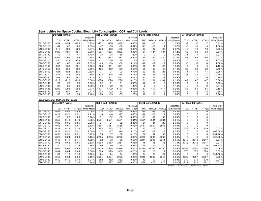
II-60

Sensitivities for Space Cooling Electricity Consumption, COP and Coil LoadsDel Qtot (kWh,e) Del Qcomp (kWh,e) Del Q IDfan (kWh,e) Del Q ODfan (kWh,e)

Abs(Max- Abs(Max- Abs(Max- Abs(Max-TUD HTAL1 HTAL2 Min)/ Mean TUD HTAL1 HTAL2 Min)/ Mean TUD HTAL1 HTAL2 Min)/ Mean TUD HTAL1 HTAL2 Min)/ Mean

E110-E100 -454 -454 -453 0.25% -431 -430 -430 0.33% -16 -16 -16 1.73% -7 -7 -7 0.31%E120-E110 -64 -66 -66 4.35% -47 -50 -50 6.37% -11 -11 -11 1.97% -5 -5 -5 1.30%E120-E100 -518 -520 -520 0.37% -478 -480 -480 0.40% -27 -27 -27 0.37% -13 -13 -13 0.35%E130-E100 -1420 -1421 -1421 0.09% -1224 -1225 -1225 0.08% -134 -134 -134 0.12% -63 -63 -63 0.07%E140-E130 -42 -41 -41 1.42% -38 -38 -38 1.22% -2 -2 -2 0.29% -1 -1 -1 2.97%E140-E110 -1007 -1009 -1009 0.18% -831 -833 -833 0.24% -120 -120 -120 0.10% -56 -56 -56 0.02%E150-E110 130 129 129 0.89% 111 110 110 1.11% 13 13 13 0.84% 6 6 6 1.63%E160-E150 -66 -67 -68 2.32% -49 -50 -50 3.14% -12 -12 -12 0.09% -6 -6 -6 1.80%E165-E160 357 360 361 0.92% 328 331 331 0.85% 20 20 20 1.56% 9 9 9 1.15%E170-E150 -565 -569 -569 0.60% -466 -469 -469 0.69% -68 -68 -68 0.40% -32 -32 -32 0.45%E180-E150 -124 -124 -125 0.62% -91 -91 -92 0.73% -22 -23 -23 0.68% -11 -11 -11 0.95%E180-E170 442 445 444 0.69% 375 378 378 0.76% 45 45 45 0.48% 21 21 21 0.40%E185-E180 462 461 461 0.21% 432 431 431 0.27% 21 21 21 0.89% 10 10 10 0.20%E190-E180 -917 -918 -918 0.08% -770 -770 -770 0.10% -101 -101 -101 0.10% -47 -47 -47 0.08%E190-E140 96 96 96 0.60% 82 81 81 0.55% 10 10 10 0.56% 5 5 5 0.53%E195-E190 87 86 86 1.38% 80 79 79 1.32% 5 5 5 1.10% 2 2 2 3.94%E195-E185 -1292 -1293 -1293 0.07% -1121 -1122 -1121 0.06% -117 -117 -117 0.20% -55 -55 -55 0.12%E195-E130 142 141 141 0.77% 123 122 123 0.76% 12 12 12 0.92% 6 6 6 0.50%E200-E100 -55 -53 -54 2.48% -70 -69 -69 1.78% 10 11 11 1.84% 5 5 5 2.28%

Sensitivities for COP and Coil LoadsDelta COP (kWh,t) Del Q coil,t (kWh,t) Del Q coil,s (kWh,t) Del Qcoil,lat (kWh,t)

Abs(Max- Abs(Max- Abs(Max- Abs(Max-TUD HTAL1 HTAL2 Min)/ Mean TUD HTAL1 HTAL2 Min)/ Mean TUD HTAL1 HTAL2 Min)/ Mean TUD HTAL1 HTAL2 Min)/ Mean

E110-E100 0.99 0.99 0.99 0.06% -35 -35 -35 0.85% -35 -35 -35 0.85% 0 0 0E120-E110 0.21 0.21 0.21 1.41% -16 -16 -17 3.65% -16 -16 -17 3.65% 0 0 0E120-E100 1.20 1.20 1.20 0.20% -51 -52 -52 0.86% -51 -52 -52 0.86% 0 0 0E130-E100 -0.50 -0.48 -0.48 3.98% -3581 -3581 -3581 0.01% -3581 -3581 -3581 0.01% 0 0 0E140-E130 0.86 0.86 0.86 0.08% -21 -21 -22 2.38% -21 -21 -22 2.38% 0 0 0E140-E110 -0.63 -0.61 -0.61 3.12% -3567 -3567 -3568 0.03% -3567 -3567 -3568 0.03% 0 0 0E150-E110 0.25 0.25 0.25 0.87% 752 752 753 0.10% 13 13 14 4.59% 739 739 739 0.03%E160-E150 0.21 0.21 0.21 2.09% -17 -17 -18 8.10% -17 -17 -18 6.73% 0 0 0 403.08%E165-E160 -0.90 -0.91 -0.91 0.72% 36 37 38 4.16% 36 37 38 3.65% 0 0 0 291.46%E170-E150 -0.26 -0.24 -0.24 8.16% -2285 -2286 -2286 0.03% -2285 -2286 -2286 0.03% 0 0 0 300.00%E180-E150 0.42 0.41 0.41 1.22% -22 -23 -25 9.69% -2241 -2240 -2241 0.05% 2218 2218 2217 0.07%E180-E170 0.68 0.65 0.65 3.82% 2263 2263 2261 0.08% 45 45 45 1.78% 2218 2218 2217 0.07%E185-E180 -1.20 -1.19 -1.19 0.55% 40 40 40 0.61% 40 40 40 0.48% 0 0 0 198.53%E190-E180 -0.66 -0.63 -0.63 4.05% -3918 -3918 -3916 0.04% -1330 -1330 -1330 0.05% -2588 -2587 -2586 0.06%E190-E140 0.64 0.64 0.64 0.58% 380 379 380 0.26% 10 10 11 7.94% 370 370 370 0.05%E195-E190 -1.09 -1.10 -1.10 0.72% 24 24 24 1.68% 24 24 24 0.84% 0 0 0 344.58%E195-E185 -0.55 -0.54 -0.54 2.10% -3934 -3934 -3933 0.03% -1346 -1347 -1346 0.04% -2588 -2587 -2587 0.05%E195-E130 0.40 0.40 0.40 1.21% 382 382 382 0.03% 12 12 12 0.89% 370 370 370 0.04%E200-E100 1.23 1.23 1.23 0.14% 1697 1697 1697 0.00% 476 476 476 0.01% 1221 1221 1221 0.01%

i220401a.xls r :s145..ak192; 05/18/01

II-61

2.5 References for Part II

These are references for Sections 2.1 and 2.2. References for Section 2.3 are included at the end of eachanalytical solution report (see end of 2.3.1 and 2.3.2).

ASHRAE Handbook of Fundamentals. (2001). Atlanta, GA: American Society of Heating, Refrigerating,and Air-Conditioning Engineers.

Dürig, M. (2000a). Hochschule Technik + Architektur Luzern. E-mail communications with J. Neymark.March 2000.

Dürig, M. (2000b). Hochschule Technik + Architektur Luzern. E-mail communication with J. Neymark.March 15, 2000.

Dürig, M., Glass, A., and Zweifel, G. (2000). Analytical and Numerical Solution for Cases E100–E200.Based on Test Description September 1998 Edition. Hochschule Technik + Architektur Luzern. Draft,August 2000.

Glass, A. (2000). Hochschule Technik + Architektur Luzern. E-mail communications with J. Neymark.February 14, 2000, and others from February–March 2000.

Knabe, G., and H-T. Le. (2000). Analytical Solution HTA Luzern - TU Dresden. Technische UniversitätDresden. 17 Mar 2000. Submitted at Madrid, Spain, March 2000. Note: This document erroneouslyindicated TUD used an atmospheric pressure of 100,000 Pa for psychrometric calculations; the actualvalue was 101,000 Pa. See Le 2000.

Le, H-T. (2000). Technische Universität Dresden. E-mail communication with J. Neymark. June 20,2000.

Le, H-T., and G. Knabe. (1998). HVAC BESTEST: Results of Analytical Solutions. Dresden University ofTechnology. E-mail from Le to Judkoff. June 19, 1998.

Le, H-T., and G. Knabe. (1999a). Solutions Techniques for Dry Coil Conditions, “Analytical Solutions forCase E110.” Dresden University of Technology. Fax from Le to Neymark. May 19, 1999.

Le, H-T., and G. Knabe. (1999b). Solutions Techniques for Dry Coil Conditions, “Analytical Solutionsfor Case E170.” Dresden University of Technology. Fax from Le to Neymark. April 30, 1999.

Zweifel, G. and Dürig, M. (1999). Analytical and Numerical Solution for Cases E100–E200. Based onTest Description September 1998 Edition. Hochschule Technik + Architektur Luzern. Draft, May 1999.

2.6 Abbreviations and Acronyms for Part II

ASHRAE American Society for Heating, Refrigerating, and Air-Conditioning Engineers

COP Coefficient Of performance

EDB Entering Dry-Bulb temperatureEWB Entering Wet-Bulb temperature

HTAL Hochschule Technik + Architektur Luzern

II-62

HTAL1 Analytical solution results by HTAL

HTAL2 Initial HTAL “numerical” solution technique applying realistic controller with 1-stimestep

IDB Indoor Dry-Bulb temperature

IEA International Energy Agency

Mean Average of TUD, HTAL 1, and HTAL2 solutions

Max Maximum of TUD, HTAL1, and HTAL2 solutions

Min Minimum of TUD, HTAL1, and HTAL2 solutions

SHC Solar Heating and Cooling (Programme)

TUD Technische Universität Dresden; in Section 2.4 this refers specifically to analyticalsolution results by TUD

PART III:

Production ofSimulation Results

III-1

3.0 Part III: Production of Simulation Results

3.1 IntroductionIn this section we describe what the working group members did to produce example results with severaldetailed programs that were considered to represent the state of the art for building energy simulation inEurope and the United States. The objectives of developing the simulation results were:

• To demonstrate the applicability and usefulness of the Building Energy Simulation Test forHeating, Ventilating, and Air-Conditioning Equipment Models (HVAC BESTEST) test suite

• To improve the test procedure through field trials

• To identify the range of disagreement that may be expected for simulation programs relative to theanalytical solution results that constitute a reliable set of theoretical results for these specific testcases (see Part IV).

The field trial effort took about 3 years and involved several revisions to the HVAC BESTESTspecifications and subsequent re-execution of the computer simulations. The process was iterative in thatexecuting the simulations led to the refinement of HVAC BESTEST, and the results of the tests led to theimprovement and debugging of the programs. This process underscores the importance of InternationalEnergy Agency (IEA) participation in this project; such extensive field trials, and resulting enhancementsto the tests, were much more cost effective with the participation of the IEA Solar Heating and Cooling(SHC) Programme Task 22 experts.

Table 3-1 describes the programs used to generate the simulation results. Appendix III (Section 3.9) presentsreports written by the modelers for each simulation program.

The tables and graphs in Part IV present the final results from all the simulation programs and analyticalsolutions used in this study. The analytical solution results constitute a reliable set of theoretical results.Therefore, the primary purpose of including simulation results for the E100–E200 cases in Part IV is toallow simulationists to compare their relative agreement (or disagreement) with the analytical solutionresults versus the relative agreement of the Part IV simulation results with the analytical solution results(i.e., a comparison with the state of the art in simulation). Perfect agreement among simulations andanalytical solutions is not necessarily expected. The Part IV results give an indication of what sort ofreasonable agreement is possible between simulation results and the analytical solution results.

Acronyms used in Sections 3.2 through 3.6 are given in Section 3.7. References cited in Section 3.2 through3.6 are given in Section 3.8.

3.2 Selection of Simulation Programs and Modeling Rules for SimulationsThe countries participating in this IEA task made the initial selections of the simulation programs used inthis study. The selection criteria required that:

• A program be a true simulation based on hourly weather data and calculational time increments of1 hour or less

• A program be representative of the state of the art in whole-building energy simulation as defined bythe country making the selection.

The modeling rules were somewhat different (more stringent) for the simulation programs used for Part IVexample results than for a given program to be normally tested with HVAC BESTEST (see Section 1.2.2,Modeling Rules). For the Part IV simulation results, we allowed a variety of modeling approaches.However, we required that these cases be modeled in the most detailed way possible for each simulationprogram within the limits of the test specification (e.g., detailed component data are not given for thecompressor, condenser, and thermal expansion device).

III-2

Table 3-1. Participating Organizations and Computer Programs

Model Authoring organization Implemented by

CA-SIS V1 Electricité de France, France Electricité de France, France

CLIM2000 2.1.6 Electricité de France, France Electricité de France, France

DOE-2.1E-088 LANL/LBNL/ESTSC,a,b,c, USA CIEMAT,d Spain

DOE-2.1E-133 LANL/LBNL/JJH,a,b,e, USA NREL/JNA,f, USA

ENERGYPLUS 1.0.0.023 LBNL/UIUC/CERL/OSU/GARDAnalytics/FSEC/DOE-OBT,a,g,h,i,j,k

GARD Analytics, USA

PROMETHEUS Klimasystemtechnik, Germany Klimasystemtechnik, Germany

TRNSYS 14.2-TUDwith ideal controller model

University of Wisconsin, USA;Technische Universität Dresden,Germany

Technische Universität Dresden,Germany

TRNSYS 14.2-TUDwith real controller model

University of Wisconsin, USA;Technische Universität Dresden,Germany

Technische Universität Dresden,Germany

aLANL: Los Alamos National LaboratorybLBNL: Lawrence Berkeley National LaboratorycESTSC: Energy Science and Technology Software Center (at Oak Ridge National Laboratory, USA)dCIEMAT: Centro de Investigaciones Energéticas, Medioambientales y TecnologicaseJJH: James J. Hirsch & AssociatesfNREL/JNA: National Renewable Energy Laboratory/J. Neymark & AssociatesgUIUC: University of Illinois Urbana/ChampaignhCERL: U.S. Army Corps of Engineers, Construction Engineering Research LaboratoriesiOSU: Oklahoma State UniversityjFSEC: University of Central Florida, Florida Solar Energy CenterkDOE-OBT: U.S. Department of Energy, Office of Building Technology, State and Community Programs, Energy Efficiency andRenewable Energy

To minimize the potential for user error, we encouraged more than one modeler to develop input files foreach program. This was done for DOE-2.1E (USA/Spain). Where disagreement in the inputs or results wasfound, we requested that the two modelers resolve the differences. Where only a single modeler wasinvolved, we strongly recommended that another modeler familiar with the program check the inputscarefully.

3.3 Improvements to the Test Specification as a Result of the Field TrialsBased on comments by the other IEA SHC Task 22 participants during the field trials, observations fromour own DOE-2.1E.simulations, and comments by industry engineers, we made a number ofimprovements and revisions to the test specification. Although researching the comments andcommunicating specification revisions to the field trial participants was very time-consuming, theimportance of the accuracy and clarity of the test specification for this type of work cannot be overstated.

The contribution of the IEA SHC Task 22 participating countries was particularly valuable because theTask 22 experts supplied continuous feedback throughout the 3-year field trial effort. Their feedbackresulted in several revisions to the HVAC BESTEST specifications and subsequent re-execution of thecomputer simulations. This iterative process led to refinement of HVAC BESTEST, and the results of the

III-3

tests led to the improvement and debugging of the programs. The process underscores the leveraging ofresources for the IEA countries participating in this project. Such extensive field trials, and resultingenhancements to the tests, would not have occurred without the participation of the IEA SHC Task 22experts.

Revisions to HVAC BESTEST were isolated in various addenda to the original (and subsequent) user’smanuals (Neymark and Judkoff 1998–2000). Most of the revisions outlined below were made during theearlier stages of the project.

• Improved description of manufacturer performance data included:

o Fan heat assumed by the manufacturer (which is not equal to the listed fan power)o Additional tables that list gross capacities and adjusted net capacitieso Clarification text about the validity of listed performance data, instructions for

interpolation and extrapolation, and instructions for modeling dry coil conditionso Clearer definition of part load ratio (PLR) and adjustment of the COP=f(PLR)

(performance degradation, CDF) curve.

• General test specification improvements included:

o Improved glossary and overall improvement in definition of termso Use of a draw-through rather than a blow-through indoor fano Adjustment of load inputs to achieve Air-Conditioning and Refrigeration Institute (ARI)

conditionso Notation of relative humidity of the weather data, along with a discussion about the

weather-data solar time conventiono Modeling rules that require consistent modeling methods (rather than most detailed

modeling methods), and clarification of model initialization and simulation periodo Clarification about thermostat control strategyo Operating assumptions that include: perfectly mixed zone air, zone loads distributed

evenly throughout the zone, no system hot gas bypass, and no compressor unloading.

• Additional equivalent inputs included:

o Discussion of bypass factor with a calculation appendixo Indoor fan performance data with a calculation appendixo Evaporator coil detailso Minimum supply air temperature.

3.4 Examples of Error Trapping with HVAC BESTEST DiagnosticsThis section summarizes a few examples that demonstrate how the HVAC BESTEST procedure was used toisolate and correct bugs in the reference programs. Further description may be found in the individual codereports presented in the next section.

Simulations were performed for each test case with the participating computer programs using four sets ofhourly typical meteorological year (TMY) weather data modified to give constant outdoor dew pointtemperature and constant outdoor dry bulb temperature (ODB) for 3 consecutive months. These artificialweather data were applied because they allow steady-state analysis, which facilitated the development ofanalytical solutions for comparison with simulation results. At each stage of the exercise, output data fromthe simulations were compared to each other according to the diagnostic logic of the test cases (see Part I,Appendix F). In the final stages of the exercise, the analytical solutions were compared. The test diagnosticsrevealed (and led to the correction of) bugs, faulty algorithms, input errors, or some combination of those inevery one of the programs tested. Several examples follow.

III-4

3.4.1 DOE2.1E Version W-54 (NREL)DOE-2 is a whole-building simulation program, the development of which has been sponsored by the U.S.Department of Energy (DOE). NREL used DOE-2.1E’s RESYS2 (residential system) for its model.

3.4.1.1 Minimum Supply Temperature Bug in RESYS2 (36% compressor+ODfanconsumption issue)In the earliest stage of the HVAC BESTEST test specification development and testing (around August of1994, before the IEA SHC Task 22 began), a problem was identified for the RESYS2 system in a versionolder than DOE-2.1E W-54. Identical input decks (for a much different preliminary version of the testspecification) were used—the only difference between the input decks was the designation of the DOE-2SYSTEM-TYPE as PSZ versus RESYS2. Table 3-2 and Figure 3-1 show the comparison results.

Table 3-2. DOE-2.1E. Version W-54 System Disagreements: RESYS2 versus PSZ

DOE-2.1ESystem

Compra+ODb fanElec.c (kWh)

Total Coil Clg.d

(kWh)Latent Clg.(kWh)

“COP”e

PSZ 2,587 7,532 1,202 2.9

RESYS2 1,646 7,767 1,524 4.8aCompr = compressorbOD = outdoorcElec = electricity consumptiondClg. = total evaporator coil loade“COP” = (Total Coil Clg.)/(Compr+ODfan Elec.)

Figure 3-1. DOE-2.1E RESYS2 minimum supply temperature bug

In response to this 36% consumption difference and the unreasonably high COP for the RESYS2 result, thecode author explained that a bug had been found in the RESYS2 system model. In that model, when theindoor fan mode is set to INTERMITTENT, the capacity calculation that sets the minimum supplytemperature (TCMIN) used the wrong value, resulting in the unrealistically high COP for the RESYS2. The

0

2000

4000

6000

8000

10000

Compr+

Odfan E

l. (kW

h)

Total c

oil lo

ad (k

Wh)

Laten

t coil

load

(kWh)

"COP"

kWh/

y th

erm

al

0

1

2

3

4

5

CO

P

RESYS2 PSZ

III-5

program authors corrected this coding error (Hirsch 1994). This is an example of how systematic checkingfor internal consistency among outputs required by HVAC BESTEST led to the discovery of an error.

3.4.2 DOE2.1E JJH Version 133 (NREL)This summary is for the version of DOE-2.1E distributed by James J. Hirsch & Associates, Camarillo,California, USA. NREL used DOE-2.1E’s RESYS2 (residential system) for its model.

3.4.2.1 Issues Transmitted to Code AuthorsFor DOE-2.1E, some disagreements and inconsistencies were also discovered.

• Fan heat discrepancy (up to 5% total coil load inconsistency at low sensible heat ratio [SHR]); morediscussion of this is included with the DOE-2.1E ESTSC version 088 summary of CIEMAT’sresults (below).

• The indoor (ID) fan does not precisely cycle on/off with compressor (2% total consumptiondisagreement at mid-PLR).

• COIL-BF-FT multiplier insensitivity (1% total consumption disagreement for E185).

The code authors have been notified about these issues, which are covered in more detail in the DOE-2.1E/NREL modeler report.

3.4.2.2 Changes from Version 117 to Version 133Before January 10, 2000, the preliminary DOE-2.1E simulation work was done with an older version (117,current version = 133). The simulation work spotted two problems (listed below) in the older version. Notethat although these problems were already fixed for version 133, they still existed in many previousversions—if there had been a systematic test in place sooner, we may have been able to address theseproblems sooner.

• Minimum entering wet bulb (EWB) was “hardwired” at 60°F (3% consumption disagreement fordry coil E110).

• Bypass factor f(PLR) multiplier = 0.99 at full load (should be 1.00); 0.4% total consumptiondisagreement for mid-PLR case E170.

For the hardwired minimum EWB issue see Figure 3-2 for a comparison of results from case E110 forversion 117, version 133, and the analytical solutions. To help visualize the differences, the y1-axisminimum has been raised and the ID fan energy was multiplied by 5. See the DOE-2.1E/NREL modelerreport for more detail on these issues.

III-6

Case E110 Results

500600700800900

1000

Compressor + OD Fan (kWh)

ID Fan (kWh) x 5

Humidity Ratio (kg/kg)

kWh

00.0020.0040.0060.0080.01

Hum

idity

Rat

io (k

g/kg

)

DOE2-jjh117 DOE2-jjh133 Analytical Soln. TUD/HTAL

Figure 3-2. Release of Hardwired EWBmin = 60°F for Case E110

3.4.3 DOE2.1E ESTSC Version 088 (CIEMAT)This summary applies to the version of DOE-2.1E distributed by the Energy Science and TechnologySoftware Center of Oak Ridge National Laboratory, Oak Ridge, Tennessee, USA. CIEMAT used DOE-2.1E’s PTAC (Packaged Terminal Air Conditioner) system for its model.

3.4.3.1 Issues Transmitted to Code AuthorsTwo issues were identified for the code authors:

• The ID fan does not precisely cycle on/off with compressor (2% total consumption disagreement atmid-PLR); this is the same problem that NREL found for the RESYS2 system in the JJH version.

• There is a “fan heat” discrepancy (up to 2% sensible coil load inconsistency at low SHR).

In terms of the fan heat discrepancy, in all cases except E130 and E140, fan heat (fan energy consumption)was not equal to sensible cooling coil load minus sensible zone load. Table 3-3, developed by CIEMAT,indicates these fan heat differences for each case.

A fan heat modeling error, or some other inconsistency between DOE-2.1E’s LOADS and SYSTEMSsubroutines, could cause this output problem.

Although both NREL and CIEMAT observed this problem, the observed discrepancy for their modelsdiffered. CIEMAT gave the following possible reasons for the differences between CIEMAT’s andNREL’s observed differences, including:

• Use of PTAC versus RESYS2

• Blow-through fan for PTAC, versus draw-through fan for RESYS2 which also:o Affects supply air temperatureo Requires minor differences in curve fit data input for performance equivalence

• Different input methods for fan performance parameterso NREL: KW/CFM and DELTA-To CIEMAT: static pressure and efficiency.

III-7

Note: NREL’s earlier sensitivity tests indicate that this is not likely to be the source of thedifference.

Table 3-3. Sensible Coil Load versus Sum of Sensible Zone Load and Fan Consumption forDOE-2.1E PTAC System

C A S ES E N S C O IL

L O A D S E N S R O O M L O A D +

S U P P L Y F A N E N E R G Y E R R O RE 1 0 0 3 8 4 1 .4 7 3 7 9 9 .6 0 5 1 .1 0 %E 1 1 0 3 8 0 3 .5 8 3 7 6 8 .5 1 8 0 .9 3 %E 1 2 0 3 7 6 3 .4 8 3 7 4 0 .0 5 3 0 .6 3 %E 1 3 0 2 1 5 .7 7 8 2 1 5 .6 6 0 .0 5 %E 1 4 0 1 9 5 .5 3 1 9 5 .4 5 0 .0 4 %E 1 5 0 3 8 0 3 .5 8 3 7 6 8 .5 1 8 0 .9 3 %E 1 6 0 3 7 7 7 .1 7 8 3 7 4 9 .5 0 4 0 .7 4 %E 1 6 5 3 8 2 8 .2 5 8 3 7 8 8 .5 4 9 1 .0 5 %E 1 7 0 1 4 8 6 .8 5 7 1 4 7 9 .4 7 3 0 .5 0 %E 1 8 0 1 5 5 3 .1 8 4 1 5 2 8 .8 6 5 1 .5 9 %E 1 8 5 1 6 0 8 .0 9 4 1 5 7 1 .9 0 5 2 .3 0 %E 1 9 0 2 0 3 .0 0 7 2 0 2 .6 4 1 0 .1 8 %E 1 9 5 2 2 5 .6 4 2 2 5 .0 5 4 0 .2 6 %E 2 0 0 4 3 1 3 .1 7 6 4 2 6 9 .6 5 3 1 .0 2 %

0 .8 1 %M E A N E R R O R

ERROR = [(sens.zone load+fan energy)–(sens.coil load)]/(sens.zone load + fan energy)*100%

3.4.4 TRNSYS-TUD with Realistic Controller (TUD)TRNSYS is considered to be the most advanced program that DOE has sponsored for simulating activesolar systems. Originally written at the University of Wisconsin, Technische Universität Dresden (TUD)acquired a license for the source code and has since developed new source code for TUD’s own calculationroutines. This new version is designated TRNSYS-TUD, and some new routines developed at TUD weretested for this project. For this project TUD ran two different TRNSYS simulation models: one with anideal controller and one with a realistic controller. The problems described below occurred in the model thatincorporated the realistic controller.

3.4.4.1 Problem with Use of Single Precision Variables (45% total consumptiondisagreement at low PLR, 14% disagreement at mid-PLR)For the initial set of TRNSYS-TUD results at low part loads (cases E130, E140, E190, and E195), large(43%–48%) errors were found in the sensible and latent coil loads; these errors also propagated through toenergy consumption predictions. For the mid-PLR case E170, the error was also high (at 14% for energyconsumption).

Diagnostic logic indicated that the problem could be with the application of the part load curve. On furtherreview, the code authors discovered a problem with the use of single-precision variables in one of thecalculation subroutines associated with the model that applies a realistic system controller. This causedrounding errors that became worse as PLR decreased.

Figure 3-3 documents the results of TUD's simulations before and after this problem was fixed. The figureincludes a comparison with TUD's analytical solution results and shows that when the appropriate variableswere changed to double-precision variables, the simulation results improved a great deal.

III-8

Figure 3-3. TRNSYS-TUD single precision variable bug

3.4.4.2 Wrong Data Compiled for Latent Coil Load Output (3% latent coil disagreementfor E170, 4% total consumption disagreement for E150, E160)After repairing the single-precision variable problem from March 1999, the September 1999 results forTRNSYS with the realistic controller showed that the latent coil load was 3% less than the latent zone loadfor case E170 (mid-PLR; see Figure 3-4). After checking by TUD—a review that also indicated 4% energyconsumption variation from their analytical solution results for cases E150 and E160—an error was foundand corrected. Quoting from TUD’s modeler report:

A type (module) is used to save the entering dry bulb temperature (EDB) and the entering humidity ratio(EHR) for calculation of the equipment performance. This type was called at the end of every timestepbut before the printer. By calling of this type all the defined equations in [the subroutine] are updated.After that the printer prints the just updated values. So the results were inconsistent. This type has beenset now after the printer and it works well.

Interestingly, two iterations were necessary to fix this error. TUD’s first attempt to fix the problem indicatedimproved agreement for some outputs. However, the results summary for March 2000 indicated that forcase E170 (mid-PLR), their latent coil load was 6% greater than their latent zone load (NREL 2000). Forthe next cycle of results they went back, undid their previous code revision, and incorporated the final fix(described above; Le 2000). The new TRNSYS-TUD results for the realistic controller now give muchbetter agreement with the analytical solution results. This iterative process underscores the diagnostic powerof HVAC BESTEST for ensuring that the problem that needed correction got corrected.

As a result of the fix, latent coil loads now match latent zone loads for all cases. Figure 3-4 illustrates theincremental improvements to TUD’s software where “Qtotal” signifies total energy consumption and “Qcoillatent” signifies latent coil load. Note that compensating errors initially (in March 1999) showed agreementfor E150 total consumption.

0

50

100

150

200

E130 low PLR, dry E190 low PLR, wetTota

l Ele

ctric

Con

sum

ptio

n (k

Wh,

Feb

ruar

y)TRNSYS-TUD with Realistic Controller - Single PrecisionTRNSYS-TUD with Realistic Controller - Double PrecisionAnalytical Solution

III-9

Figure 3-4. TRNSYS-TUD data gathering bug fix

3.4.4.3 Additional Observations about Diagnosing the TRNSYS ErrorsIt is interesting to observe, in the case of the second TRNSYS-TUD error, that only after the first error wasfixed did the second error became apparent. This classic example of how some errors mask others furtherunderscores the utility of the HVAC BESTEST diagnostics in being able to uncover both problems.

Additionally, the second example indicates the enhanced robustness of having an analytical truth standard.Although the error was initially flagged by the inconsistency among the latent coil loads and latent zoneloads, the consumption errors were not apparent because at the time we had no agreeing analyticalverification solutions and because of noise among the simulation results. Only after the TUD code authorscompared their TRNSYS results with their own analytical solution (which yielded results very close to thefinal analytical solutions) were they able to identify the important discrepancies in the consumption resultsthat initiated this revision.

3.4.5 CLIM2000 (EDF)CLIM2000, developed by the French national electric utility Electricité de France (EDF), is an advancedmodular building energy simulation software program.

Four different models were used in this study:

• The initial set of results used an older mechanical system model. Previous validation exercises hadmade EDF aware of some problems with this model. The code authors submitted results for twopossible modeling methods appropriate to that model (see “CLIM2000-1a” and “CLIM2000-1b” inFigure 3-5).

• The second set of results used a new mechanical system model on which development had begunbefore this validation project started. The new model was completed midway through this project(see “CLIM2000-2” in Figure 3-5).

• The third and fourth sets of results incorporated improvements to the new model that resulted fromwork on this project (see “CLIM2000-3” and “CLIM2000-4” in Figure 3-5).

0200400600800

10001200

Qtotal

E150:

hiSHR

Qtotal

E160:

as15

0 hiID

B

Qcoil la

tent: E

170 m

SHR mPLR

kWh

TRNSYS Real Ctrl3/99TRNSYS Real Ctrl9/99TRNSYS Real Ctrl3/00TRNSYS Real Ctrl6/00Analytical SolutionHTAL/TUD

III-10

Figure 3-5 summarizes the results of the different models, along with the analytical solutions of TUD/Hochschule Technik + Architektur Luzern (HTAL). Details on analysis of the results and changes to themodels are given in the sections that follow.

Figure 3-5. CLIM2000 new model comparison and improvements

3.4.5.1 Evaluation of the New Mechanical Equipment Model (up to 50% COP effect)From these results, it is apparent that EDF's new mechanical equipment model (designated by “CLIM2000-2”) is a big improvement over the previous model (for most but not all cases—see E195). The previousmodel had up to 50% disagreement in the worst case (E140 low PLR, low ODB). Also, the new model wasable to model case E185 (high latent load); the old model was the only simulation that was unable to modelthat case. Using BESTEST in this way—where the changes to the model are already in progress—ensuresthat intended changes are actually made. From Figure 3-5, it is apparent that much of the intendedimprovement did occur, however, some problems remained as described in the next sections.

3.4.5.2 No COP=f(PLR) Sensitivity (20% consumption disagreement at low PLR, 13%disagreement at mid-PLR)The results for the second set of runs indicated that the new model was not sensitive to performance (COP)degradation at part load. Figure 3-6 (extracted from EDF's modeler report) gives COP sensitivitycomparison for the new model, a comparison that indicates there is no COP=f(PLR) sensitivity. Seeespecially the highlighted (arrows) results in Figure 3-6 (i.e., for E130–E100, E140–E110, E190–E180, andE195–E185). These all check the PLR effect over default conditions as described in the appendix to Part Ion diagnostic logic. (Note: In Figure 3-6, “BESTEST3” in the header above the graph is EDF’s designatorfor the same set of results that we have called “CLIM2000-2” in Figure 3-5.)

012345

E100 d

ry lo

IDB hi

ODB

E110 a

s100

lo O

DB

E130 a

s100

lo PLR

E140 a

s130

lo O

DB

E170 a

s110

mSHR m

PLR

E185 l

oSHR hi

ODB

E195 a

s185

loPLR

E200 A

RI PLR

=1 hiSHR

CO

P

CLIM2000-1a CLIM2000-1b CLIM2000-2 (no f(PLR))CLIM2000-3 CLIM2000-4 Analytical TUD/HTAL

III-11

Mean COP sensitivities - CLIM2000 Results (BESTEST3)

-2.00

-1.50

-1.00

-0.50

0.00

0.50

1.00

1.50

2.00

E110-E

100

E120-E

110

E120-E

100

E130-E

100

E140-E

130

E140-E

110

E150-E

110

E160-E

150

E165-E

160

E170-E

150

E180-E

150

E180-E

170

E185-E

180

E190-E

180

E190-E

140

E195-E

190

E195-E

185

E195-E

130

E200-E

100

Del

ta C

OP

Figure 3-6. Mean COP sensitivities—CLIM2000-2 results

Figure 3-5 indicates that the lack of sensitivity gives a 20% COP (or consumption) error at low PLR (E130,E195), and a 13% error at mid-PLR (E170). These errors occurred because no COP degradation for cyclingwas implemented in the model. Based on these results, EDF decided to implement COP degradation for partload cycling into CLIM2000. In the “CLIM2000-3” results, the part load COP has better agreement (asindicated in Figure 3-5; especially notice cases E130, E140, E170, and E195).

3.4.5.3 Improved Performance Map Interpretation (up to 9% consumption effect for drycoils [E110])After EDF completed its third set of results, there remained 7% and 10% disagreements in totalconsumption versus the analytical solutions for cases E100 and E110, respectively. In EDF’s fourthmodeling, the code authors improved CLIM2000’s interpretation of the performance data by automatingdata extrapolation with EWB, including recognition of dry coil conditions, and manually extrapolating forEDB. Their results for the dry-coil cases are now within 1% of the analytical solutions. Results of thisimprovement are designated by CLIM2000-4 in Figure 3-5; especially notice cases E100 and E110 in thefigure.

3.4.5.4 Comments on Compensating Errors and DiagnosticsThe agreement for CLIM2000-2 in E100 caused by compensating errors is noteworthy. It is interesting tosee how the correction for PLR is indicated as needed in other cases (e.g., E140) but not indicated as neededin E100, even though it should have been (although to a lesser degree than in E140). When the insensitivityto PLR was corrected in the CLIM2000-3 results, the E100 results then helped reveal a performance mapinterpretation error in CLIM2000-3 (previously concealed in E100, but perhaps not in E110).

Also, CLIM2000-2 has good agreement in cases E200 and E185—full load and near-full-load cases withmoderate and high latent loads (high and low SHR), respectively—that do not test either sensitivity to partloading or operation at dry coil conditions. Because of their character, cases E200 and E185 are notsensitive to the algorithmic changes by EDF after CLIM2000-2, although they were useful in identifyingproblems with CLIM2000-1.

III-12

It is apparent, then, that it is the variety of cases founded by the diagnostic logic associated with HVACBESTEST that allows a greater number of possible errors to be identified—even those errors that maysometimes be concealed by compensating disagreements.

3.4.6 CA-SIS (EDF)CA-SIS is the whole-building hourly simulation program that EDF developed and used for building energystudies. The calculation engine for CA-SIS is the TRNSYS solver, property of the University ofWisconsin’s Solar Energy Laboratory (USA), marketed in France by CSTB (Centre Scientifique etTechnique du Batiment).

EDF used three different sets of simulations in this study:

1) The initial set of results featured:

a. No extrapolation of the performance map

b. No accounting for fan heat in the coil load

c. No accounting for CDF in the energy consumptions of the compressor, indoor fan, andoutdoor fan—although the initial results indicate COP sensitivity to part loading, EDF citescompensating errors as the cause (Hayez 2000)

d. Zone humidity ratio variation between time steps limited using mathematical relaxation tobe able to run all cases and to improve convergence (see the CA-SIS modeler report[Appendix III-D]).

2) The second set of results featured the following differences from the first set:

a. Manual extrapolation of the performance data

b. Accounting for fan heat in the coil load

c. Accounting of CDF for the compressor

d. Additional parameter variation between time steps limited using mathematical relaxation(zone humidity [more limited than before], zone temperature, and envelope load) for caseE200; see the CA-SIS modeler report (Appendix III-D).

3) The third set of results featured the following differences from the second set:

a. Revised manual extrapolation of the performance data including dry coil performancelimits

b. Accounting of CDF for indoor and outdoor fans

c. Zone temperature variation between time steps was limited using mathematical relaxationfor all cases.

The COP results for these models, along with the TUD/HTAL analytical solution results, are summarized inFigure 3-7. Figure 3-8 includes specific results used to diagnose the causes for various disagreements;relevant outputs have been scaled for convenience so that we could include them all in this figure. As aresult of this modeling and analysis work, the following specific problems were identified for CA-SIS.

III-13

Figure 3-7. COP improvements to CASIS models

Figure 3-8. CASIS fixes: fan heat, fan CDF, and convergence algorithm

3.4.6.1 Fan Heat Not Included in Total Coil Load (4% sensible coil load effect for allcases)In Figure 3-8 it is apparent from the CA-SIS 2/00 results for sensible coil load (shown by the group ofresults labeled “E165 Q Coil Sens”) that sensible coil load was about 4% lower than the analyticalsolution results. This difference was seen in all the sensible coil load outputs and was traced to fan heatnot being accounted for in the coil load. After fan heat was included in the coil load (see “CA-SIS 6/00”results), the sensible coil loads agreed with the analytical solution results. Because multiple changes weremade between the first and second models (see above) and because of probable compensating errors, it

0

500

1000

1500

2000

E165 QCoil Sens

÷ 3

E170 QIDfan x 20

E170 QODfan x

20

E200 QCoil Latent

kWh

CASIS 2/00 CASIS 6/00CASIS 10/00 Analytical TUD/HTAL

1.52

2.53

3.54

4.5

E100 d

ry lo

IDB hi

ODB

E110 a

s100

lo O

DB

E120 a

s100

hiID

B

E130 a

s100

lo PLR

E140 a

s130

lo O

DB

E165 h

iSHR mID

B mODB

E170 a

s110

mSHR m

PLR

E180 a

s150

loSHR

E185 l

oSHR hi

ODB

E190 a

s180

loPLR

E195 a

s185

loPLR

E200 A

RI PLR

=1 hi

SHR

CO

P

CASIS 2/00 CASIS 6/00CASIS 10/00 Analytical TUD/HTAL

CASIS 2/00Case E200 did not converge

III-14

was not possible to isolate this effect in the compressor power results. However, the effect onconsumption should also reasonably have been 4% for dry coil cases, and less than that for wet coil cases(decreasing with decreasing SHR).

3.4.6.2 Indoor and Outdoor Fan Power Did Not Include COP=f(PLR) Degradation (2%total consumption effect at mid PLR)In Figure 3-8, it is apparent from the “CA-SIS 2/00”and “CA-SIS 6/00” results for indoor fan energy (shownby the group of results labeled “E170 Q IDfan × 20” and “E170 QODfan × 20”), that indoor fan energyconsumption was about 12% lower than the analytical solution results for case E170. These differenceswere traced to CDF not being accounted for in the indoor and outdoor fan consumptions. This has a 2%effect on total energy consumption for these cases, and would have a higher percentage of effect at a lowerPLR (and a lower percentage of effect at a higher PLR).

3.4.6.3 Convergence Algorithm (E200, full load case, could not be run)The Figure 3-7 COP results for the group labeled “E200 ARI” and Figure 3-8 results for the group labeled“E200 Q Coil Latent” do not indicate results for “CA-SIS 2/00” case. This is because initially CA-SIS hadconvergence problems for case E200, and could not run it. To fix the problem, in its second run of E200,EDF applied limits to variation between time steps (using mathematical relaxation) to the followingparameters: zone humidity ratio (more limited than before), zone temperature, and envelope load. With thischange, the E200 COP results in Figure 3-7 are improved. EDF has also changed the default value of acoefficient used in CA-SIS’s convergence algorithm.

The E200 latent coil load results in Figure 3-8 indicate an error in the calculation of latent coil load. Thisremaining latent coil load disagreement turns out to have been related to improper extrapolation of theperformance map (Hayez 2000). For its third CA-SIS simulation, EDF revised the performance map inputsfor CA-SIS to indicate the limits of performance for dry coil conditions. Integrating this new performancemap resulted in an agreeing latent coil load for the CA-SIS 10/00 results, as shown in Figure 3-8.

3.4.6.4 No Automated Extrapolation of Performance Data (possibly up to 10%consumption effect in E110)In the initial “CA-SIS 2/00” results, the COP for all the dry-coil cases differs from the TUD analyticalsolutions by 0.04 to 0.20 units of COP (1.2%–7.3%); see especially case E140 in Figure 3-7. The dry-coilcases require a small degree of extrapolation, as well as careful attention to which of the given manufacturerdata points correspond to wet coil conditions (all valid data) and which correspond to dry coil conditions(and do not give valid compressor consumptions and total capacities). In the “CA-SIS 6/00” simulations,EDF manually extrapolated the performance data and input those data to CA-SIS again to obtain newresults. Figure 3-7 indicates that for some cases, this had no effect. For other cases (e.g., E100 and E130),COP varied such that there was still disagreement. Because the “CA-SIS 6/00” runs also included otheradjustments (see above), it is difficult to say if this change was solely responsible for the variation.

For the “CA-SIS 10/00” results, the manual extrapolation was improved to include the difference inbehavior between dry coil and wet coil conditions on the performance map. For this set of results, the CA-SIS COPs give much better agreement with the analytical solution results. Because the first try at manualextrapolation may have been errant, and because EDF did not present individual sensitivity tests of eachchange in its modeler report, it is difficult to state exact quantitative effects of performing extrapolations inthe CA-SIS results. However as shown in the CLIM2000 modeler report, EDF’s CLIM2000 results forE110 and E100 indicate that 7%–10% error in total energy consumption is possible when smallextrapolations of the performance data are not performed.

III-15

3.4.7 EnergyPlus (GARD Analytics)EnergyPlus is the program recently released by DOE, and is the building energy simulation program thatwill be supported by DOE. GARD Analytics (GARD) used EnergyPlus’s “Window Air-Conditioner”system for its model.

GARD submitted eight iterations of simulation results. Table 3-4 describes input file and softwaremodifications for each iteration; a single results set was submitted corresponding to changes described ineach row of the table. Version Beta 5-07 was used for the initial results set.

Table 3-4. Summary of EnergyPlus Changes That Were Implemented

Version Input File Changes Code ChangesBeta 5-07Beta 5-12through

Beta 5-14

• DX coil calculations modified to account for cycling• Modified method of calculating SHR and coil bypass

factorBeta 5-15through

Beta 5-18

• Changed DX (direct expansion) coil objectnames

• Changed name of DX coil object to better representits algorithmic basis(no impact on results)

Ver 1-01throughVer 1-11

• Changed from blow-through to draw-throughfan configuration

• Changed to double precision• Modified method of calculating coil outlet

conditions• Added draw-through fan option to Window Air-

Conditioner modelVer 1-12throughVer 1-14

• New equipment performance curves• Adjusted fan mass flow and efficiency to achieve

desired mass flow and fan powerVer 1-15throughVer 1-17

• Went back to specified values for fan mass flowand efficiency

• Partial implementation of moist air specific heat• Fan power calculated using a standard initial density

for volume to mass flow conversionVer 1-18throughVer 1-19

• Changed basis of CDF curve from net to gross• Opened up minimum/maximum limits for

performance curves

• Complete implementation of moist air specific heat• Heat of vaporization (hfg) calculation modified for

latent loadsVer 1-20throughVer 1-23

• Went back to original CDF curve (modifiedcurve used with Version 1-19 was incorrect)

• Changed from FAN:SIMPLE:CONSTVOLUMEto FAN:SIMPLE:ONOFF

• Used CDF curve for fan power to account forcycling

• Implemented optional PLR curve for fan cycling• Changed moisture initializations to use outdoor

humidity ratio

The COP results for selected cases are summarized in Figure 3-9 for the EnergyPlus simulations and theTUD/HTAL analytical solution results. Note that the differences in results have been magnified in thisfigure by increasing the minimum value on the y-axis. Figure 3-10 includes specific results used to diagnosethe causes of various disagreements. For the initial run with Beta 5-07, a number of disagreements with theanalytical solution results were identified:

• Low indoor fan electrical power and fan heat; see Figure 3-10 results labeled “E170 Q ID Fan x 50”

• Reported cooling coil loads apparently not adjusted for part load cycling (although actual loadremoved from the zone appears to have been adjusted); see Figure 3-10 results labeled “E140 QCoil Total”

• Sensible coil load about 1% higher than total coil load in the dry-coil cases.

III-16

2.002.503.003.504.004.50

E110 d

ry lo

IDB/O

DB

E120 a

s110

hi ID

B

E140 a

s110

lo PLR

E150 a

s110

hi SHR

E170 a

s150

mSHR/PLR

E180 a

s 150

lo SHR

E190 a

s 180

lo PLR

E200 A

RI PLR

=1 hi

SHR

CO

P

Beta 5-07 Beta 5-14 Ver 1-11 Ver 1-17Ver 1-19 Ver 1-23 Analytical

Figure 3-9. COP improvements to EnergyPlus models

Figure 3-10. EnergyPlus fixes: various results

The process of correcting these disagreements engendered the improvements to EnergyPlus describedbelow.

3.4.7.1 Reported Cooling Coil Loads Not Adjusted for Part Load Operation (up to2500% effect on total coil load, negligible effect on energy consumption)In Figure 3-10 it is apparent from the Beta 5-07 results for total coil load (designated by the results labeled“Q Coil Total” for cases E140, E170, and E200) that the total cooling coil load is in error, with the greatesterror found in cases with lower PLR. For Beta 5-14 the reporting of cooling coil loads was corrected toaccount for run time during cycling operation. Because for Beta 5-07 the actual load extracted from thespace was already being adjusted for cycling (similar magnitude disagreements do not exist for COP ofcases E140 and E170 in Figure 3-9), it appears that this problem had a negligible effect on COP and energyconsumption.

0

1000

2000

3000

4000

5000

6000

E140 QCoil Total

E170 QCoil Total

E200 QCoil Total

E200QSens

Coil-Zone x20

E180 QCoil Latent

E170 Q IDFan x 50

kWh

Beta 5-07 Beta 5-14 Ver 1-11 Ver 1-17Ver 1-19 Ver 1-23 Analytical

III-17

3.4.7.2 Modified Calculation of SHR and BF (1%–2% total consumption effect)The problem of sensible coil loads being greater than total coil loads was addressed by modifying themethods of calculating SHR and BF. With the reasonable assumption that the coil load reporting errorhad negligible effect on energy consumption, the difference in COP between Beta 5-14 and Beta 5-07(shown in Figure 3-9) illustrates the 1%–2% energy consumption effect of this modification, with asimilar degree of change for all cases.

Along with the remaining differences in COP that are apparent from Figure 3-9 for Beta 5-14, GARD noteda number of other disagreements that were previously masked:

• Total coil loads were generally greater than for the analytical solutions (see “E200 Q Coil Total”results in Figure 3-10), and were 1%–2% greater than the sums of total zone load plus fan energyconsumption

• The mean IDB for E200 moved from 26.7°C (good) to 27.1°C (high)

• Previous Beta 5-07 disagreements in terms of low ID fan power remain (see “E170 Q ID Fan × 50”results in Figure 3-10).

These disagreements with the analytical solutions prompted further improvements, described below.

3.4.7.3 Draw-through Fan, Double-Precision Variables, and Modified Calculation of CoilOutlet Conditions (0.1%–0.7% total consumption effect)Changes leading up to Version 1-11 included:

• Modified method for calculating coil outlet conditions

• Use of double precision throughout EnergyPlus (this change was prompted by other issues notrelated to HVAC BESTEST)

• Addition of draw-through fan option to the window air-conditioner system.

Unfortunately, the effects of each of these changes were not disaggregated in the testing. The combinedeffects of these changes are illustrated in Figure 3-10, where the results for Beta 5-14 are compared to thosefrom Ver 1-11 for the set of results labeled “E200 Qsens Coil-Zone × 20” (the difference between sensiblecoil loads and sensible zone loads, magnified by a factor of 20). This set of results indicates a 5% change inthe loads-based calculated fan heat. The overall effect of these changes on COP (and consumption) is <1%as illustrated in Figure 3-9 comparing the difference between results of Ver 1-11 and Beta 5-14.

Along with remaining differences in COP apparent for Ver 1-11 in Figure 3-9, GARD noted otherremaining disagreements:

• Total coil load remained 1%–2% greater than total zone load plus fan heat; similarly, the latent coilloads were 3% greater than for the analytical solution results—see “E180 Q Coil Latent” results inFigure 3-10

• The mean IDB for E200 moved from 27.1°C (high) to 27.5°C (higher)

• Previous Beta 5-07 disagreements of low ID fan power became worse compared with analyticalsolution results (see “E170 Q ID Fan × 50” results in Figure 3-10).

3.4.7.4 Change to Standard Air Density for Fan Power Calculation (1% decrease insensible coil load)For versions 1-12 through 1-17, results for changes to the software were aggregated with input file changes(notably the revision of system performance curves) so that assessing the effect of software revisions—including the implementation of moist air specific heat and the use of standard air properties for calculatingsupply air mass flow rates—was difficult. However, in Figure 3-10 (for the set of results labeled “E200

III-18

Qsens Coil-Zone × 20” for Ver 1-17 versus Ver 1-11), the bulk of the remaining fan heat discrepancyappears to have been addressed in version 1-17 when the fan power calculation was changed to incorporatestandard air density. This change appears to have resulted in a 1% change in sensible and total coil load (seeresults for “E200 Q Coil Total” in Figure 3-10). The effect on ID fan energy appears to be about 3% (seeresults for “E170 ID Fan Q × 50” for Ver 1-17 versus Ver 1-11 in Figure 3-10), which translates to a 0.3%total power effect. The total electricity consumption effect would be greater in cases where the fan isrunning continuously (e.g. because of outside air requirements) even though the compressor is operating atlower part loads.

3.4.7.5 Modified Heat of Vaporization for Converting Zone Latent Load into HVACSystem Latent Load (0.4%–2.5% total consumption effect for wet coil cases only)For versions 1-18 and 1-19, the effects of input file changes were likely negligible (CDF curve revision), orthe changes may have only affected specific cases. Enabling extrapolation of performance curves appears tohave had the greatest effect in E120—see Figure 3-9 results for E120, Ver 1-19 versus Ver 1-17. Therefore,changes in results for the wet coil cases are likely caused primarily by changes to the software. Versions 1-18 through 1-19 include the following changes to the software:

• Changed heat of vaporization (hfg) used for converting a zone latent load into a coil load

• Changed airside HVAC-model specific heat (cp) from dry air to moist air basis.

From Figure 3-10, the case E180 latent coil load results (designated by “E180 Q Coil Latent”) for Ver 1-19versus Ver 1-17 indicate that the fixes to the software improved the latent coil load results, with a 4% effecton latent coil load for E180 and the other wet coil cases (not shown here). In Figure 3-9, the differencebetween Ver 1-19 and Ver 1-17 illustrates the effect on COP, with the greatest effect (2.2%–2.5%) seen forcases with the lowest SHR (e.g., cases E180 and E190). GARD also noted that changing the airside HVAC-model specific heat (cp) from a dry air to a moist air basis improved consistency between coil and zone loadsand removed other small discrepancies.

3.4.7.6 ID Fan Power Did Not Include COP f(PLR) Degradation (2% total consumptioneffect at mid PLR)In Figure 3-10, using the set of results labeled “E170 Q ID Fan × 50” (fan energy use magnified by a factorof 50), it is apparent that indoor fan consumption was about 15% lower than the analytical solution resultsfor case E170. This difference was traced to CDF not being accounted for in the ID fan consumption.Application of COP=f(PLR) was implemented by Ver 1-23, and better agreement with the analyticalsolution indoor fan energy consumption was the result. The difference in results for Ver 1-23 and Ver 1-19in Figure 3-9 indicates a 2% effect on total energy consumption for the mid-PLR case E170, with a higherpercentage of effect as PLR decreases (e.g., see Figure 3-9 results for case E140 or E190).

3.4.7.7 General Comment About Improvements to EnergyPlusEach individual error found in EnergyPlus by itself did not have >3% effect on consumption results. However, these multiple errors do not necessarily compensate each other, and may be cumulative in somecases. Furthermore, some errors that have small effect on total consumption for these cases (e.g. fan modelerrors when the indoor fan is cycling with the compressor) could have larger effects on total consumptionfor other cases (e.g., if the indoor fan is operating continuously while the compressor cycles). Therefore,correcting these errors was important.

3.4.8 PROMETHEUS (KST)PROMETHEUS is a whole-building hourly simulation program developed and used by Klimasystemtechnik(KST) of Berlin, Germany, for the company’s energy and design consulting work.

III-19

During September 1998, the PROMETHEUS modelers reported that the CDF was externally applied toPROMETHEUS. The significance of CDF to the simulation results is documented in the CLIM2000 resultssummary (presented earlier in this section). As a result of this work the code authors planned to implement aCOP=f(PLR) algorithm into PROMETHEUS (Behne 1998). However, because KST was unable toparticipate in the project after January 2000, it was unable to complete the refinement of its simulationresults.

III-20

Results, Conclusions, andRecommendations

III-21

3.5 Interpretation of ResultsThe tables and graphs in Part IV present the final results from all the simulation programs and analyticalsolutions used in this study. Because the analytical solution results constitute a reliable set of theoreticalresults (a mathematical truth standard), the primary purpose of including simulation results for the E100–E200 cases in Part IV is to allow simulationists to compare their relative agreement (or disagreement) withthe analytical solution results. Perfect agreement among simulations and analytical solutions is notnecessarily expected. The Part IV results give an indication of what sort of agreement is possible betweensimulation results and the analytical solution results.

As we have explained previously, the analytical solution results do not represent absolute truth; instead, theyrepresent a mathematical truth standard for cases E100–E200. Given the underlying physical assumptions inthe case definitions, the analytical solutions are a mathematically provable and deterministic result for eachcase. In this context the underlying physical assumptions about the mechanical equipment as defined incases E100–E200 are representative of typical manufacturer data, normally used by building designpractitioners, with which many whole-building simulation programs are designed to work.

It is important to reiterate the difference between a mathematical truth standard and an absolute truthstandard. In the former we accept the given underlying physical assumptions while recognizing that theseassumptions represent a simplification of physical reality. The ultimate or absolute validation standardwould be comparison of simulation results with a perfectly performed empirical experiment, the inputs forwhich are perfectly specified to the simulationists. In reality an experiment is performed and theexperimental object specified within some acceptable band of uncertainty. Such experiments are possiblebut fairly expensive. We recommend that a set of empirical validation experiments be developed for futurework.

One must rely on engineering judgment to assess the significance of results that disagree. For simulationresults that disagree significantly with the analytical solution results, investigating the source(s) of thedifference(s) is worthwhile, but the existence of a difference does not necessarily mean that a program isfaulty. However, our collective experience in this task has indicated that when programs show disagreementwith analytical solution results, other simulation results, or both, we often find a bug or a questionablealgorithm.

As expected, because of iterative correction of input errors, software bugs, and clarification of the testspecification, the quality of simulation results improved with each iteration of the field trials. Improvementsto the simulation programs are evident when the initial results set is compared to the current results set.Initial simulation results for COP obtained after the first round of simulations, before the analyticalsolutions were developed, are shown in Figure 3-11 (abbreviations along this graph’s x-axis areshorthand for the case descriptions given in Part I). These results indicate that there was initially 2%–30% average disagreement versus the mean of the simulated COP results. Corresponding disagreementof energy consumption results ranged from 4%–40%.

Figure 3-12 includes the current set of COP results for all the simulations and analytical solutions;abbreviations along this figure’s x-axis are the same as in Figure 3-11. After correcting software errorsusing HVAC BESTEST diagnostics, the mean results of COP and total energy consumption for theprograms are, on average, within <1% of the analytical solution results, with average variations of up to2% for the low PLR dry coil cases (E130 and E140).

III-22

Figure 3-11. HVAC BESTEST—mean COP, before BESTESTing

(Abbreviations along the x-axis are shorthand for the case descriptions; see Part I for full casedescriptions.)

Figure 3-12. HVAC BESTEST—mean COP, after BESTESTing

(Abbreviations along the x-axis are shorthand for the case descriptions; see Part I for full casedescriptions.)

0

0.5

1

1.5

2

2.5

3

3.5

4

4.5

E100:

dry lo

IDB hi

ODB

E110:

as10

0 lo O

DB

E120:

as10

0 hiID

B

E130:

as10

0 lo P

LR

E140:

as13

0 lo O

DB

E150:

as11

0 hiSHR

E160:

as15

0 hiID

B

E165:

as15

0 mID

B mODB

E170:

as11

0 mSHR m

PLR

E180:

as15

0 loS

HR

E185:

loSHR hi

ODB

E190:

as18

0 loP

LR

E195:

as18

5 loP

LR

E200:

ARI PLR

=1 hi

SHR

CO

P

DOE-2.1E/NREL DOE-2.1E/CIEMAT TRNSYS 14.2/TUD CLIM2000-A/EDFCLIM2000-B/EDF Prome-A/KST Prome-B/KST

0

0.5

1

1.5

2

2.5

3

3.5

4

4.5

E100 d

ry lo

IDB hi

ODB

E110 a

s100

lo O

DB

E120 a

s100

hiID

B

E130 a

s100

lo PLR

E140 a

s130

lo O

DB

E150 a

s110

hiSHR

E160 a

s150

hiID

B

E165 a

s150

mID

B mODB

E170 a

s150

mSHR m

PLR

E180 a

s150

loSHR

E185 l

oSHR hi

ODB

E190 a

s180

loPLR

E195 a

s185

loPLR

E200 A

RI PLR

=1 hi

SHR

CO

P

CASIS/EDF CLIM 2000/EDF DOE-2.1E/CIEM AT DOE-2.1E/NREL ENERGY+/GARD PROM ETHEUS/KSTTRNSYS-ideal/TUD TRNSYS-real/TUD Analytical/TUD Analytical/HTAL1 Analytical/HTAL2

III-23

Ranges of disagreement are further summarized in Table 3-5 for predictions of various outputs. Thisrange of disagreement for each case is based on the difference between each simulation result versus themean of the analytical solution results, divided by the mean of the analytical solution results. The outputsare disaggregated for dry coil performance (no dehumidification) and for wet coil performance(dehumidification moisture condensing on the coil). This summary excludes results for thePROMETHEUS participants; although they suspected an error(s) in their software, they were unable tocomplete the project.

Table 3-5. Ranges of Disagreementa among Simulation Results

Cases

Dry Coil

(E100-E140)

Wet Coil

(E150-E200)

COP and Total ElectricConsumption

0% - 6%a 0% - 3%a

Zone Humidity Ratio 0% - 11%a 0% - 7%a

Zone Temperature 0.0°C - 0.7°C (0.1°C)b

0.0°C - 0.5°C (0.0°C – 0.1°C)b

a Percentage disagreement for each case is based on the difference between each simulation result (excluding PROMETHEUS) versus the mean of the analytical solution results, divided by the mean of the analytical solution results. b Excludes results for TRNSYS-TUD with realistic controller.

The higher level of disagreement in the dry coil cases, which occurs for the case with the lowest PLR, isrelated to some potential problems that have been documented for DOE-2.1E (ESTSC version 088 andJJH version 133) in both the CIEMAT and NREL results (see Section 3.4). The larger disagreements forzone humidity ratio were caused by disagreements for the CLIM2000 and DOE-2.1E/CIEMAT results.The disagreement in zone temperature results is primarily from the TRNSYS-TUD results, where arealistic controller was applied on a short timestep (36 s); all other simulation results applied idealcontrol.

Based on results after “HVAC BESTESTing,” the programs appear reliable for performance-mapmodeling of space cooling equipment when the equipment is operating close to design conditions. In thefuture, HVAC BESTEST cases may explore modeling at “off-design” conditions and the effects of usingmore realistic control schemes.

3.5.1 Test Cases for Future WorkIn the course of this work it became apparent from comments of the participants and observations of the testspecification authors that some additional test cases would be useful for improved error trapping anddiagnostics with HVAC BESTEST. In future work, we suggest that some extensions to the test suite,outlined in the sections that follow, be considered.

3.5.1.1 Mechanical EquipmentCompletion of the proposed E300-series cases (Neymark and Judkoff 2001) is the highest priority. Thesecases will not be possible to solve analytically, but will be developed as comparative test cases. They aredynamic test cases that utilize unrevised dynamic annual site weather data. They also help to scale thesignificance of disagreements that are less obvious with steady-state test cases. The cases test the ability tomodel the following:

• Quasi-steady-state performance using dynamic boundary conditions: dynamic internal gainsloading, and actual (dynamic) typical meteorological year 2 (TMY2) weather data

III-24



• Periods of operation away from typical design conditions





• ODB and EDB performance sensitivities (using dynamic loading and dynamic weather data).

The proposed E300-series cases also address the important question of the ability of simulation software tomodel equipment performance at off-design conditions. These cases include a set of expanded performancedata (beyond what is normally provided with typical manufacturer catalog data) and may include a test ofthe ability to extrapolate from a set of typical manufacturer catalog performance data.

It would also be interesting to add cases with more realistic control schemes. Such cases could include:

• Five-minute minimum on/off or hysteresis control, or both. Preliminary work by TUD documentedin the TRNSYS-TUD modeler report suggests that it might be interesting to try:

o Case E140 with 5-min minimum on and 5-min minimum offo Case E130 with 2°C hysteresiso Five-minute minimum off (a common manufacturer setting)o Combination of minimum on/off and hysteresiso Proportional controlo Adding equipment run time to outputs

• Variation of part load performance based on more detailed data.

Other cases that are either under development or being considered for development as part of IEA SHCTask 22 involve:

• Heating equipment such as furnaces, heat pumps

• Radiant floor slabs for heating and cooling.

Additional possible cases include:

• Variable-air volume fan performance and control

• Outside dew point temperature (humidity ratio) effect on performance (see the DOE-2.1E/NRELmodeler report [Appendix III-A])

• Repeat one or two of the E100–E200 series cases using expanded performance data

• Fan heat testing using continuous fan operation at low compressor part load

• PLR testing using ARI conditions for ODB, EWB, and EDB

• Combination of mechanical equipment tests with a realistic building envelope (although combiningthese adds noise, which makes diagnostics more difficult).

Obtaining additional simulation results would also be useful. Possible additional programs to test include:ESP, FSEC 3.0, HVACSIM+, the American Society of Heating, Refrigerating, and Air-ConditioningEngineers (ASHRAE) HVAC2 Toolkit, and others.

For the longer term, there has been discussion of trying to gather data that would allow highly detailedequivalent primary-loop component models of, for example, compressors, condensers, evaporators, andexpansion valves, to be incorporated into the test specification. Incorporating and verifying data for such

III-25

models to enhance the current HVAC BESTEST specification is expected to be a major effort. Additionallong-term work would also include:

• Thermal storage equipment

• Air-to-air heat exchanger

• More complex systems associated with larger buildings including:

o Large chillerso Chilled water loopso Cooling towers, and related circulation loopso More complex air handling systemso Other “plant” equipment

• ASHRAE RP-865 air-side analytical test field trials.

3.5.1.2 EnvelopeIEA SHC Task 22 is updating reference results for existing IEA envelope BESTEST (Judkoff and Neymark1995a) and HERS BESTEST (Judkoff and Neymark 1995b) cases with ground-coupled heat transferthrough floor slabs and basement walls. Task 22 is also considering development of cases to test the abilityto model multizone envelope heat transfer (Kataja and Kalema 1993).

Based on comments about this project and previous work, we can identify a number of other interestingareas relating to envelope models for which BESTEST cases could be developed. These include:

• Expanded ground coupling cases

• Expanded infiltration tests (e.g., testing algorithms that vary infiltration with wind speed)

• Varying radiant fraction of heat sources

• Moisture adsorption/desorption

• Daylighting controls.

ASHRAE has developed a series of envelope analytical tests under RP-1052 (Spitler, Rees, and Dongyi2001). Future work could also include field trials of these tests.

Finally, the current IEA BESTEST envelope tests should be updated periodically to include:

• New simulation results for the current set of programs and also other simulation results from, forexample, APACHE, CA-SIS, CLIM2000, EnergyPlus, ESP, SUNREL, TRNSYS

• Application of updated TMY2 weather data

• Additional radiative exchange tests (see Table 2-51 of IEA BESTEST, Judkoff and Neymark1995a).

3.6 Conclusions and Recommendations

3.6.1 ConclusionsAdditional test cases for mechanical space cooling equipment have been added to IEA's existing method forsystematically comparing whole-building energy software and determining the algorithms responsible forprediction differences. Similar to previous test suites that applied the HVAC BESTEST method, these newcases have a variety of uses, including:

III-26

• Comparing output from building energy simulation programs to a set of analytical solutions thatconstitutes a reliable set of theoretical results given the underlying physical assumptions in the casedefinitions

• Comparing several building energy simulation programs to determine the degree of disagreementamong them

• Diagnosing the algorithmic sources of prediction differences among several building energysimulation programs

• Comparing predictions from other building energy programs to the analytical solutions andsimulation results in this report

• Checking a program against a previous version of itself after the internal code has been modified, toensure that only the intended changes actually resulted

• Checking a program against itself after a single algorithmic change to understand the sensitivitybetween algorithms.

The previous IEA BESTEST envelope test cases (Judkoff and Neymark 1995a) have been code-language-adapted and formally approved by ANSI and ASHRAE as a Standard Method of Test, ANSI/ASHRAEStandard 140-2001. The BESTEST procedures are also being used as teaching tools for simulationcourses at universities in the United States and Europe.

Adding mechanical equipment tests to the existing envelope tests gives building energy software developersand users an expanded ability to test a program for reasonableness of results and to determine if a programis appropriate for a particular application. The current set of steady-state tests (cases E100–E200) representsthe beginning of work in this area. A set of additional cases has been proposed; these new (E300-series)cases are briefly described in Section 3.5.1, where additional cases for future consideration beyond the E300series are also discussed.

Part II of this report includes analytical solution results for all the cases. Because the analytical solutionresults constitute a reliable theoretical solution and the range of disagreement among the analytical solutionsis very narrow compared to the range of disagreement among the simulation results, the existence of theanalytical solutions improves the diagnostic capability of the cases. This means that a disagreeingsimulation result for a given test implies a stronger possibility that there is an algorithmic problem, codingerror, or input error than when results are compared only with other simulation programs.

The procedure has been field-tested using a number of building energy simulation programs from the UnitedStates and Europe. The method has proven effective at isolating the sources of predictive differences. Thediagnostic procedures revealed bugs, faulty algorithms, limitations, and input errors in every one of thebuilding energy computer programs tested in this study—CA-SIS, CLIM2000, DOE-2.1E, ENERGYPLUS,PROMETHEUS, and TRNSYS-TUD. Table 3-6 summarizes the notable examples.

Many of the errors listed in Table 3-6 were significant, with up to 50% effect on total consumption or COPfor some cases. In other cases for individual programs, some errors had relatively minor (<2%) effect ontotal consumption. However, where a program had multiple errors of smaller magnitude, such errors did notnecessarily compensate each other, and may have been cumulative in some cases. Furthermore, some errorsthat have small effect on total consumption for these cases (e.g., a fan heat calculation error when the indoorfan is cycling with the compressor), could have larger effects for other cases not included with the currenttests, but planned for later tests (e.g. if the indoor fan were operating continuously, independent ofcompressor cycling). Therefore, correcting the minor errors as well as the major errors was important.

III-27

Table 3-6. Summary of Software Problems Found Using HVAC BESTEST

Software Error Descriptiona % Disagreementa,b ResolutionCA-SIS No extrapolation of performance data allowed Possibly up to 10% powerc

(E110, E100)Manuallyfixedd

CA-SIS Convergence algorithm problem E200 would not run FixedCA-SIS Fan heat not added to coil load 4% sensible coil load ([4%

powerc f(SHR)e)Fixed

CA-SIS Indoor and outdoor fan power not f(PLR) 2% powerc (mid PLR) FixedCLIM2000 Verify new model improvementsf Up to 50% COP change from

earlier modelVerifiedimproved

CLIM2000 Compressor and fan powers exclude COP = f(PLR)degradation

20% powerc (low PLR)13% powerc (mid PLR)

Fixed

CLIM2000 Performance map extrapolation problem 9% powerc (E110) FixedDOE-2.1E (JJH ver< W54)

Minimum supply temperature coding error in earlyRESYS2g system

36% COP (earlier base caseh) Fixed

DOE-2.1E(JJH ver 133)

Coil-Zone load difference disagrees with fan powerfor RESYS2g at low SHR.

5% sensible coil load (at lowSHR)

Authorsnotified

DOE-2.1E (JJH ver133)

Bypass factor = f(EWB, ODB) insensitivity 1% powerc (E185) Authorsnotified

DOE-2.1E (JJH133, ESTSC 088)

Indoor fan power not f(PLR) (RESYS2 and PTAC)g 2% total power (at mid PLR) Authorsnotified

DOE-2.1E(ESTSC v 088)

Coil-Zone load difference disagrees with fan powerfor PTACg at low SHR.

2% sensible coil load (at lowSHR)

Authorsnotified

ENERGYPLUS Reported coil loads not f(PLR) Up to 2500% coil load (at lowPLR); 0% powerc

Fixed

ENERGYPLUS Calculation of SHR and bypass factor 1-2% powerc FixedENERGYPLUS Heat of vaporization for latent coil calculation 0.4-2.5% powerc FixedENERGYPLUS Indoor fan power not f(PLR) 2% powerc (mid PLR) FixedPROMETHEUS Compressor COP = f(PLR) calculated in external

post-processor to software20% powerc (low PLR) if nopost-processor calc.

Authorsnotified

TRNSYS-TUD(realistic control)

Use of some single precision variables 45% powerc (lo PLR)14% powerc (midPLR)

Fixed

TRNSYS-TUD(realistic control)

Wrong data compiled for coil latent load output. 4% powerc (E150)3% latent coil load (E170)

Fixed

a Acronyms used in this column are described in the Nomenclature.b Specific cases or conditions relevant to the described disagreement are included in parenthesis.c Total system powerd Current results include non-automated version of the fix.e Percentage disagreement is greatest at high SHR and decreases as SHR decreases.f The software authors used HVAC BESTEST to document the improvement of their new model relative to a previous

model that they were in the process of replacing when IEA SHC Task 22 began.g In DOE-2.1E the RESYS2 system is for modeling typical residential equipment (e.g. a unitary split system), and PTAC is

for modeling a packaged terminal air-conditioning system.h This error was discovered using a preliminary version of HVAC BESTEST which had a base case different from E100.

Performance of the tests resulted in quality improvements to all the building energy simulation programsused in the field trials. Many of the errors found during the project stemmed from incorrect codeimplementation; however, there were also instances where no algorithm existed internal to a program toaccount for equipment performance degradation with decreasing part-load ratio (PLR). Some of thesebugs may well have been present for many years. The fact that they have just now been uncovered showsthe power of BESTEST and also suggests the importance of continuing to develop formalized validationmethods. It is only after coding bugs have been eliminated that the assumptions and approximations inthe algorithms can be evaluated where necessary.

III-28

Checking a building energy simulation program with HVAC BESTEST requires about 1 person-week for anexperienced user. (This estimate is based on a poll of the participants, and does not include time forfinding/fixing coding errors or revising documentation.) Because the simulation programs have taken manyyears to produce, HVAC BESTEST provides a very cost-effective way of testing them. As we continue todevelop new test cases, we will adhere to the principle of parsimony so that the entire suite of BESTESTcases may be implemented by users within a reasonable time span.

After using HVAC BESTEST diagnostics to correct software errors, the mean results of COP and totalenergy consumption for the programs are, on average, within <1% of the analytical solution results, withaverage variations of up to 2% for the low PLR drycoil cases (E130 and E140). This summary excludesresults for one of the participants, who suspected an error(s) in their software but was unable to completethe project. Based on results after HVAC BESTESTing, the programs appear reliable for performance-map modeling of space cooling equipment when the equipment is operating close to design conditions.

Manufacturers typically supply catalog equipment performance data for equipment selection at given design(near-peak) load conditions. Data for off-design conditions, which can commonly occur in buildings withoutside air requirements or high internal gains, are not included. In practice, simulation tools often use datafrom the manufacturer to predict energy performance. In general, the current generation of programsappears most reliable when performance for zone air and ambient conditions that occur within the bounds ofthe given performance data is being modeled. However, preliminary sensitivity tests indicate significantdifferences in results when extrapolations of performance data are required. Additional cases have beenproposed to explore simulation accuracy at off-design conditions (Neymark and Judkoff 2001). Thosecases, which are in the field-trial process, include a set of expanded performance data beyond what isnormally provided with typical manufacturer catalog data. Obtaining such expanded performance datarequired significant effort. We reviewed three equipment selection software packages typically used byHVAC engineers for specifying equipment. However, none of these were satisfactory for developing therange of data we desired, so the data we ultimately obtained was custom-generated by a manufacturer. Ingeneral for the state of the art in annual simulation of mechanical systems to improve, manufacturers need toeither readily provide expanded data sets on the performance of their equipment, or improve existingequipment selection software to facilitate generation of such data sets.

Within the BESTEST structure, there is room to add new test cases when required. BESTEST is betterdeveloped in areas related to energy flows and energy storage in the architectural fabric of the building.BESTEST work related to mechanical equipment is still in its early phases. Near-term continuing work(E300-series cases, not included in this report) is focused on expanding the mechanical space cooling casesto include:

• Dynamic performance using dynamic loading and actual (dynamic) TMY2 weather data



• Periods of system operation away from typical design conditions





• ODB and EDB performance sensitivities (using dynamic loading and weather data).

For the longer term we hope to add test cases that emphasize special modeling issues associated with morecomplex building types and HVAC systems as listed in Section 3.5.1.

III-29

3.6.2 RecommendationsThe previous IEA BESTEST procedure (Judkoff and Neymark 1995a), developed in conjunction withIEA SHC Task 12, has been code-language-adapted and approved as a Standard Method of Test forevaluating building energy analysis computer programs (ANSI/ASHRAE Standard 140-2001). Thismethod primarily tests envelope-modeling capabilities. We anticipate that after code-languageadaptation, HVAC BESTEST will be added to that Standard Method of Test. In the United States, theNational Association of State Energy Officials (NASEO) Residential Energy Services Network(RESNET) has also adopted HERS BESTEST (Judkoff and Neymark 1995b) as the basis for certifyingsoftware to be used for Home Energy Rating Systems under the association’s national guidelines. TheBESTEST procedures are also being used as teaching tools for simulation courses at universities in theUnited States and Europe. We hope that as the procedures become better known, developers willautomatically run the tests as part of their normal in-house quality control efforts. The large number ofrequests (more than 800) that we have received for the envelope BESTEST reports indicates that this isbeginning to happen. Developers should also include the test input and output files with their respectivesoftware packages to be used as part of the standard benchmarking process.

Clearly, there is a need for further development of simulation models, combined with a substantial programof testing and validation. Such an effort should contain all the elements of an overall validationmethodology, including:

• Analytical verification

• Comparative testing and diagnostics

• Empirical validation.

Future work should therefore encompass:

• Continued production of a standard set of analytical tests

• Development of a set of diagnostic comparative tests that emphasize the modeling issues importantin large commercial buildings, such as zoning and more tests for heating, ventilating, and air-conditioning systems

• Development of a sequentially ordered series of high-quality data sets for empirical validation.

Continued support of model development and validation activities is essential because occupied buildingsare not amenable to classical controlled, repeatable experiments. The few buildings that are truly useful forempirical validation studies have been designed primarily as test facilities.

The energy, comfort, and lighting performance of buildings depend on the interactions among a largenumber of transfer mechanisms, components, and systems. Simulation is the only practical way to bring asystems integration problem of this magnitude within the grasp of designers. Greatly reducing the energyintensity of buildings through better design is possible with the use of simulation tools (Torcellini, Hayter,and Judkoff 1999). However, building energy simulation programs will not be widely used unless the designand engineering communities have confidence in these programs. Confidence and quality can best beencouraged by combining a rigorous development and validation effort with user-friendly interfaces,minimizing human error and effort.

Development and validation of whole-building energy simulation programs is one of the most importantactivities meriting the support of national energy research programs. The IEA Executive Committee forSolar Heating and Cooling should diligently consider what sort of future collaborations would best supportthis essential research area.

III-30

3.7 Acronyms for Part IIIThese are acronyms used in Sections 3.2 through 3.6.

ARI: Air-Conditioning and Refrigeration InstituteBF: Bypass FactorCDF: COP Degradation Factor is a multiplier (≤1) applied to the full-load system COP. CDF is a function

of PLRCIEMAT: Centro de Investigaciones Energéticas, Medioambientales y TechnologicasCOP: Coefficient of Performance, the ratio using same unites of the net refrigeration effect to the cooling

energy consumption, where the net refrigeration effect is heat removed by the coil excluding thefan, heat, and cooling energy consumption is the site electricity consumption of the compressor, airdistribution fan, condenser fan, and related auxiliaries.

DOE: U.S. Department of EnergyEDB: Entering Dry-Bulb temperature, the temperature of a thermometer would measure for air entering

the evaporator coilEDF: Electricité de FranceEWB: Entering Wet-Bulb temperature, the temperature of a wet-bulb portion of a psychrometer would

measure if exposed to air entering the evaporator coilGARD: GARD AnalyticsHTAL: Hochschule Tecknik+Architektur LuzernID: IndoorIDB: Indoor Dry-Bulb temperature, the temperature a thermometer would measure if exposed to indoor

airIEA: International Energy AgencyKST: KlimasystemtechnikNREL: National Renewable Energy LaboratoryOD: OutdoorODB: Outdoor Dry-Bulb temperature, the temperature a thermometer would measure if exposed to

outdoor air; this is the temperature of the air entering the condenser coilPLR: Part Load Ratio, the ratio of net refrigeration effect to adjusted net capacity where the net capacity

is the gross total capacity of the system less the fan power (heat); gross total capacity is the rate ofboth sensible and latent heat removal by the cooling coil for a given set of operating conditions

SHC: Solar Heating and Cooling Programme (of the IEA)SHR: Sensible Heat Ratio, is the ratio of sensible heat removal to total (sensible + latent) heat removal by

the evaporator coilTMY2: Typical Meteorological Year 2TUD: Technische Universität Dresden

III-31

3.8 References for Part IIIThese are references for Sections 3.2 through 3.6. References for Appendix III are included at the end ofeach modeler report.

ANSI/ASHRAE Standard 140-2001. (2001). Standard Method of Test for the Evaluation of BuildingEnergy Analysis Computer Programs. Atlanta, GA: American Society of Heating, Refrigerating, and Air-Conditioning Engineers.

Behne, M. (September 1998). E-mail and telephone communications with J. Neymark. Klimasystemtechnik,Berlin, Germany.

Hayez, S. (November 2000). Fax and telephone communications with J. Neymark. Electricité de France,Moret sur Loing, France.

Hirsch, J. (November 1994). Personal communications. James J. Hirsch & Associates, Camarillo, CA.

Judkoff, R.; Neymark, J. (1995a). International Energy Agency Building Energy Simulation Test (IEABESTEST) and Diagnostic Method. NREL/TP-472-6231. Golden, CO: National Renewable EnergyLaboratory.

Judkoff, R.; Neymark, J. (1995b). Home Energy Rating System Building Energy Simulation Test (HERSBESTEST). NREL/TP-472-7332. Golden, CO: National Renewable Energy Laboratory.

Kataja, S.; Kalema, T. (1993). Energy Analysis Tests for Commercial Buildings (Commercial Benchmarks).IEA 12B/21C. Tampere University of Technology. Tampere, Finland: International Energy Agency.

Le, H-T. (August 2000). E-mail communication with J. Neymark. Technische Universität Dresden.

NREL. (2000). HVAC BESTEST Summary of 5th Set of Results Cases E100 - E200. Compiled by J.Neymark & Associates for NREL. Golden, CO: National Renewable Energy Laboratory.

Neymark J.; Judkoff, R. (1998–2000). Addenda to draft versions of International Energy Agency BuildingEnergy Simulation Test and Diagnostic Method for Mechanical Equipment (HVAC BESTEST). Golden, CO:National Renewable Energy Laboratory. These addenda include:

• “September 1998 Summary of Revisions to HVAC BESTEST (Sep 97 Version),” September 1998• “May 1999 Summary of Comments and Related Clarifications to HVAC BESTEST, September

1998 and February 1999 User's Manuals,” May 1999• “Revisions to E100-E200 Series Cases,” December 16, 1999• “Re: Revisions to E100 Series Cases,” e-mail from Neymark to participants January 3, 2000; 2:21

P.M.• “E100-E200 series cases,” e-mail from Neymark to participants January 3, 2000; 2:23 P.M.• “HVAC BESTEST: E100-E200 two minor but important points,” e-mail from Neymark to

participants, January 10, 2000; 8:10 P.M.

All relevant information from these addenda was included in the final version of Part I.

Neymark J.; Judkoff, R. (2001). International Energy Agency Building Energy Simulation Test andDiagnostic Method for Mechanical Equipment (HVAC BESTEST), Volume 2: E300, E400, E500 SeriesCases. Golden, CO: National Renewable Energy Laboratory. Draft. October 2001.

Spitler, J.; Rees, S.; Dongyi, X. (2001). Development of an Analytical Verification Test Suite for WholeBuilding Energy Simulation Programs—Building Fabric. Draft Final Report for ASHRAE 1052-RP.Stillwater, OK: Oklahoma State University School of Mechanical and Aerospace Engineering.

Torcellini, P.; Hayter, S.; Judkoff, R. (1999). Low Energy Building Design: The Process and a CaseStudy. ASHRAE Transactions 1999 105(2). Atlanta, GA: American Society of Heating, Refrigerating,and Air-Conditioning Engineers.

III-32

3.9 APPENDIX III: Simulation Modeler ReportsIn Appendix III, we present reports written by the modeler(s) for each simulation program. The modelerswere asked to document:

• Modeling assumptions (required inputs not explicitly described in the test specification)

• Modeling options (alternative modeling techniques)

• Difficulties experienced in developing input files for the test cases with their program

• Bugs, faulty algorithms, documentation problems, or input errors uncovered using the HVACBESTEST diagnostics

• Source code or input modifications made because of the diagnostic results

• Comments on agreement or disagreement of results compared to analytical solution and othersimulation results

• Any odd results obtained with their programs

• Sensitivity studies conducted to further understand the sources of differences between theirprograms and the others

• Conclusions and recommendations about their simulation programs, HVAC BESTEST, or both.

Modelers also filled out a pro-forma description that defines many of the algorithms within theirprograms. The pro-forma description is presented at the end of each individual modeler report. Thesepro-forma reports, which appear as they were submitted with minimal reformatting and editing, are alsopresented here.

III-33

Appendix III-A

DOE-2.1ENational Renewable Energy Laboratory/J. Neymark & Associates

United StatesJanuary 25, 2001

1. Introduction

Software: DOE-2.1E J.J. Hirsch version 133

Authoring Organization: Lawrence Berkeley National Laboratory & Los Alamos National Laboratory &J.J. Hirsch & Associates

Authoring Country: USA

Modeling Methodology:

For modeling unitary direct expansion cooling systems, DOE-2.1E uses performance maps based onmanufacturer performance data. The user may either use the default performance maps supplied with thesoftware, or generate custom performance maps based on published performance data for a specific unit.

Zone loads are calculated hourly, separately from the equipment performance. That is, DOE-2.1E firstcalculates just the loads for the entire simulation period assuming a constant zone temperature. Then itcalculates the system performance using the previously calculated hourly zone loads for the entiresimulation period, with an adjustment to the zone loads to account for the actual zone temperature providedby the mechanical system and its controls.

Overall performance for total capacity and efficiency is described as:

hourly property = (value at ARI rating conditions)*(multiplier f(EWB,ODB))*(multiplier f(PLR))

where:

ARI ≡ Air Conditioning and Refrigeration Institute

EWB ≡ Entering Wet-bulb Temperature

ODB ≡ Outdoor Dry-bulb Temperature

PLR ≡ Part Load Ratio, (Coil total energy removal)/(Gross Total Capacity)

The f(EWB,ODB) curve fits can be bilinear or biquadratic functions; the f(PLR) curve fits can be linear,quadratic or cubic. The sensible capacity also follows a similar function, however, to account for additionalvariation as a function of EDB, DOE-2 has a hardwired (not controllable by the user) assumption of:

SCAPT = ("COOL-SH-CAP")*("COOL-SH-FT"(EWB,ODB))-{1.08*CFM*(1.0-CBF)*(80-EDB)},

where:

SCAPT ≡ sensible capacity

CFM ≡ airflow rate at fan rating conditions

CBF ≡ coil bypass factor

(2.1A Reference Manual, p. IV.238).

III-34

Extrapolation of curve fits can be limited in DOE2, using either a cap on the dependent variable results, or acap on ODB and EWB. The cap on EWB is hardwired as being EWB = ODB - 10. Bypass factor alsoincludes variation as a function of fan speed.

DOE-2.1E automatically identifies when a dry coil condition has occurred and does calculationsaccordingly. F(EWB,ODB) curve fit data is meant for wet coils only. Where possible f(T) data pointsassume EDB = 80°F, however at lower EWB, it was necessary to use data for EDB < 80°F (and normalizethat data to be consistent with EDB-80°F data) to give proper information to curve fit routines; this was truefor sensible capacity and bypass factor performance maps, but not necessary for EIR or total capacity maps.

Initial zone air conditions (temperature and humidity) are the ambient conditions.

Ideal controls can be modeled. It is possible to account for minimum on/off times by adjusting f(PLR)curves. If needed the COOL-CLOSS-FPLR curve used by the RESYS2 also has a limits feature that allowsfor modeling minimum on/off system operating requirements.

The HVAC BESTEST user's manual does not give enough information for comparing component models(e.g., disaggregation of individual heat exchangers, etc.) so no attempt was made to check if specificequipment models in PLANT could have been applied to this work.

2. Modeling Assumptions

Some inputs must be calculated from the given data. For example fan power is described as kW/cfm. Suchinputs are not noted below because they are a simple calculation directly from the inputs. Those inputsnoted below are included either because they may be inferred from information in the test specification, orthe DOE-2.1E algorithms use assumptions (e.g. specific heat of air) slightly different from the testspecification

• FLOOR-WEIGHT=30: recommendation by DOE-2 for lightweight construction. This input isrelatively unimportant for the near adiabatic envelope where conduction is already < 1% of totalsensible internal gains for most cases (is about 5% in low PLR cases).

• THROTTLING-RANGE = 0.1: Minimum setting in DOE-2; exact ideal on/off control is notpossible, some proportionality is required.

• MIN-SUPPLY-T = 46: This minimum supply temperature setting is low enough so that the supplyair temperature is not limited by this input.

• SUPPLY-DELTA-T = 0.789 (is delT from fan heat): The DOE-2 Engineer's Manual indicates usingmoist air specific heat (ρ (cp) 60 = 1.10), therefore that factor was used for calculating this input.

• COIL-BF and related bypass factor f(EWB,ODB) curve: DOE-2's recommendation for calculatingbypass factors uses dry air specific heat (ρ (cp) 60 = 1.08) rather than moist air specific heat givenin the user's manual appendix. (2.1A Reference Manual, p. IV.247). The input decks therefore usedthe ρ (cp) 60 = 1.08 factor in determining leaving air conditions relevant to bypass factorcalculations.

• COOL-FT-MIN = 65 (ODB extrapolation minimum that allows extrapolation down to EWB = 55)

• MIN-UNLOAD-RATIO = 1; no compressor unloading

• MIN-HGB-RATIO = 1; no hot gas bypass

• OUTDOOR-FAN-T = 45; default, limit below which fans do not run. At this setting the fans willalways cycle on/off with the compressor for cases E100-E200.

III-35

3. Modeling Options

SYSTEM-TYPE: RESYS2 model

A number of SYSTEM-TYPEs are possible and reasonable for modeling the HVAC BESTEST DX system,including: RESYS2, RESYS, PSZ, and PTAC. Choice of system type affects: default performance curvesand features available with the system.

Of these, according to a DOE-2 documentation supplement (21EDOC.DOC), neither PTAC nor RESYShave had the improved part load (cycling) model for packaged systems incorporated (this uses the COOL-CLOSS-FPLR curve rather than the COOL-EIR-FPLR curve). Additionally, RESYS2 has more peripheralfeature options than RESYS (possibly useful later on), and one of the code authors (Hirsch) recommendedthe RESYS2 over the RESYS system type. Then either the PSZ or RESYS2 models could have workedsince custom performance curves are applied. Therefore, RESYS2 was somewhat arbitrarily chosen becauseits default performance curves should be closer to the HVAC BESTEST performance data. When RESYS2versus PSZ is used for SYSTEM-TYPE with HVAC BESTEST custom performance curves applied to bothand no other changes between the models, sensitivity tests give results that are virtually identical (novariation more significant than to the 5th significant digit, and then only for some of outputs).

SYSTEM-FANS: SUPPLY-KW & SUPPLY-DELTA-T

SYSTEM-FANS includes two different possibilities for determining indoor distribution fan power and heat. This is by either providing values for:

• SUPPLY-KW and SUPPLY-DELTA-T (rated fan power and temperature rise due to fan heat)

• SUPPLY-STATIC, SUPPLY-EFF (rated static pressure and efficiency) and SUPPLY-MECH-EFF(mechanical efficiency, only relevant if fan motor outside air stream). When the motor is located inthe air stream SUPPLY-STATIC and SUPPLY-EFF can also be the total pressure and efficiency,respectively.

Fans were modeled with SUPPLY-KW and SUPPLY-DELTA-T. However, SUPPLY-STATIC andSUPPLY-EFF could also have been used. Sensitivity test between these options using equivalent inputs o fHVAC BESTEST indicated no discernible variation in fan energy or compressor energy use, and < 0.01%effect on total coil load.

Disaggregation of indoor and outdoor fans.

The test cases indicate that compressor and fans all cycle on and off together. In developing the model withDOE-2, it is possible for the modeler to disaggregate the compressor, outdoor fan, and indoor fan, oraggregate the fans with the compressor model. When components are disaggregated, the outdoor fan seesthe exact same part load adjustment as the compressor, using the COOL-CLOSS-FPLR curve to apply theCOP Degradation Factor (CDF) indicated by the test specification. However, part load adjustment for theindoor fan does not include the CDF adjustment and is just a straight PLR multiplier. For stricter adherenceto the requirement that compressor and fans cycles on and off together, indoor and outdoor fans could havebeen modeled as aggregated with the compressor. However, the DOE-2 documentation indicates that thereis a better latent simulation with the indoor fan modeled separately from the compressor (2.1A User'sManual, p. IV.241). Additionally, disaggregation is better for diagnostic comparisons with the other results.Therefore, we decided to disaggregate the fans in the model. The effect on total energy use of the indoor fannot exactly cycling on/off with the compressor and outdoor fan is examined in Section 5.

III-36

4. Modeling Difficulties

Indoor fan is not exactly cycling on and off with compressor and outdoor fan

Indoor fan is not exactly cycling on and off with compressor and outdoor fan - see above. Also see Section5 for more detail on the relatively minor energy consumption inaccuracy caused by this.

Apparent minor inconsistency with specific heat used for calculating SUPPLY-DELTA-T and COIL-BF inputs

There is an apparent minor inconsistency with specific heat of air used for calculating COIL-BF inputsversus SUPPLY-AIR-DT. Both equations utilize the equation:

q = m (cp) ∆T, where since the flow rate is given

m = ρ * Q * 60, where Q is volumetric fan air flow rate in cfm.

So that:q = (ρ (cp) 60) * Q * ∆T.

For developing inputs the term K = "ρ (cp) 60" is used. In general for standard air ρ = 0.075 lb/ft3. For dryair cp = 0.24 Btu/lb°F resulting in K = 1.08 and for moist air w ≈ 0.01 so that cp = 0.244 Btu/lb°F resultingin K = 1.10, where K has units of (Btu*min)/(ft3*F*h). Also note that some references indicate thatstandard air is dry (e.g. ASHRAE Terminology, Howell et al) while others only specify the density butindicate the possibility that standard air can be moist (e.g. ANSI/ASHRAE 51-1985).

For initially calculating SUPPLY-DELTA-T at standard air conditions, the DOE-2.1A Engineers Manual (p.IV.29) uses moist (w=0.01) air (K = 1.10). However, for calculating the COIL-BF input (and data points forCOIL-BF-FT), the DOE-2.1A User's Manual, p. IV.247 indicates K = 1.08. Note that an HVAC textpublished by ASHRAE (Howell et al, p. 3.5) uses K = 1.10 for calculating leaving air conditions usingvolumetric air flow rates.

This is a minor inconsistency within DOE-2 that is not surprising given ambiguities in the general literature. However, it seems that if K = 1.10 is used for SUPPLY-DELTA-T, then also assuming moist air cp forcalculating leaving air conditions in determining bypass factors should be used, when giving advice for userinputs. (Note the DOE-2 Engineer's Manual indicates that DOE-2 actually adjusts ρ*cp for actual enteringconditions in the hourly calculations; so perhaps it would be appropriate to advise users to base BF inputson actual entering ρ*cp in the DOE-2 User's Manual?)

It is recommended that all these DOE-2 input requirements be made consistent with each other such that themethods for calculating the inputs are clearer to the user. An example of a good instruction format is theCOIL-BF input discussion in the DOE-2 User's Manual (2.1A, p. IV.247).

5. Software Errors Discovered and/or Comparison Between Different Versions of the Same Software

This section documents one major problem and several minor issues. Regarding minor issues, they mayseem small individually, but when summed up, they can make a difference in the aggregate results. Additionally, this documents the rigor associated with developing input decks that are as consistent aspossible with the test specification, and therefore appropriate for BESTEST reference results for later(E300-series) cases when analytical verifications will not be possible.

III-37

Fixed Bug Resulting from this Work

Minimum Supply Temperature Bug in RESYS2 (36% issue)

In the earliest stage of the HVAC BESTEST test specification development and testing (ca. 8/94 prior to thebeginning of IEA SHC Task 22), a problem surfaced for the RESYS2 system in a version prior to DOE-2.1EW-54. Identical input decks (for a much different preliminary version of the test specification) were usedwith the only difference between the input decks being the designation of SYSTEM-TYPE as PSZ versusRESYS2. The results obtained are shown in Table N1.

Table N1: RESYS2 versus PSZ for DOE-2.1E before Version W54

DOE-2 System Compr+ODfanElec. (kWh)

Coil Clg.(kBtu)

Latent Clg.(kBtu)

EER(Coil/Elec)

PSZ 2,587 25,700 4,100 9.8

RESYS2 1,646 26,500 5,200 16.1

In response to this 36% consumption difference and the unreasonably high EER for the RESYS2 result, oneof the code authors explained that that they found a bug in the RESYS2 system model. In that model, whenthe indoor fan mode is set to INTERMITTENT, the capacity calculation that sets the minimum supplytemperature (TCMIN) used the wrong value, resulting in the unrealistically high EER for the RESYS2. This coding error was corrected by the code authors (Hirsch 11/94).

Issues to Transmit to Code Authors

Fan heat discrepancy (2% issue at low SHR)

The current set of results for DOE-2.1E v133 indicates a discrepancy for fan heat calculated from:

Qfan = Qcoil,tot - Qcoil,lat - Qenv,sens

versus Qfanpower, where

Qcoil,tot ≡ total cooling energy extracted by the coil

Qcoil,lat ≡ latent cooling energy extracted by the coil

Qenv,sens ≡ sensible cooling energy extracted from the zone

Qfanpower ≡ fan electric energy consumption.

The differences in the fan heats for the various cases along with the percent effect on total coil load (andtherefore total energy consumption) are listed in Table N2.

The following is apparent from the table:

• The greatest discrepancy occurs for the high humidity cases (E180-E195) with 40% overestimationof fan heat, which is nearly 2% of total coil load.

• For the other wet-coil cases with more commonly found SHRs, there is a 10-20% overestimation offan heat, which is roughly 0.5% of total coil load.

• For the dry-coil cases the discrepancy seems insignificant, with only a 2% underestimation of fanheat, which is 0.1% of total coil load.

III-38

Table N2: Fan Heat Discrepancy d:\e\iea22\hvabtest\results\doe2\21ejna2a.xls a:a63..k87; 22 jan 01

F e b r u a r y T o t a l s

Supply Evaporator Coil Load Envelope Load Qfan,heat (del Qfan) (del Qfan)

Cases Fan Total Sensible Latent Sensible Latent Qfan,heat - Qfan /Qfan /Qcoil

(kWh) (kWh) (kWh) (kWh) (kWh) (kWh) (kWh) (kWh) (frac) (frac)

E100 141 3794 3794 0 3655 0 139 -2 -0.017 -0.001

E110 122 3756 3756 0 3637 0 119 -3 -0.025 -0.001

E120 110 3739 3739 0 3632 0 108 -2 -0.023 -0.001

E130 8 215 215 0 208 0 8 0 -0.050 -0.002

E140 6 195 195 0 188 0 6 0 0.025 0.001

E150 136 4528 3786 742 3637 739 149 13 0.090 0.003

E160 121 4508 3769 739 3632 739 137 16 0.120 0.004

E165 145 4549 3809 740 3648 739 161 16 0.097 0.003

E170 63 2237 1498 739 1419 739 79 16 0.204 0.007

E180 112 4535 1607 2928 1419 2958 188 76 0.405 0.017

E185 137 4583 1653 2930 1437 2958 215 78 0.364 0.017

E190 14 579 212 366 188 370 24 10 0.410 0.017

E195 18 602 235 367 208 370 28 10 0.347 0.016

E200 151 5522 4303 1219 4122 1221 181 30 0.166 0.005

E100R2EP 141 3794 3794 0 3655 0 139 -2 -0.015 -0.001

E180R2EP 112 4535 1607 2928 1419 2958 188 76 0.406 0.017

Additional sensitivity tests (designated by "E???R2EP" in Table N2) indicate that this problem is likely notthe result of improper entry of the fan heat temperature rise (SUPPLY-DELTA-T = 0.798), as use ofequivalent inputs SUPPLY-STATIC = 1.09 and SUPPLY-EFF = 0.5 give the same results for both fanenergy use and resulting coil and envelope loads. In addition a prior sensitivity test was run for Case E165giving the same conclusion.

ID Fan does not precisely cycle on/off with compressor (2% issue at mid-PLR)

Cycling the indoor fan on/off with the compressor is activated by inputting INDOOR-FAN-MODE =INTERMITTENT under SYSTEM-FANS. Based on detailed output, although the indoor fan is cycling, thecycling is not exactly on/off with the compressor and outdoor fan. That is, the increase runtime associatedwith use of the COOL-CLOS-FPLR curve is not applied to the indoor fan power output (SFKW).

III-39

The significance of this discrepancy is best quantified for the mid-PLR Case E170 where:

• SFKW output: 63 kWh

• SFKW if CLOSFPLR adjustment could be applied: 73 kWh.

This is then a 14% issue for the Case E170 indoor fan energy. Since for E170 Qcoil = 2237 kWh, then ifadditional fan heat is also not included, the additional coil load unaccounted for (kWh) is 10/2237 = 0.45%.Since the total compressor+fans energy is 620 kWH, the missing 10/620 + 0.45% amounts to a 2.1%underestimation of total energy use. A conversation with the manufacturer that provided performance dataand technical support for this project indicates that most small unitary systems do not have fan delays(Cawley). Therefore, because equipment often operates at part load, the RESYS2 indoor fan model shouldincorporate the part load COP degradation effect of the CLOSFPLR curve (additional operating time).

Changes from 117 to 133

The preliminary DOE-2 simulation work prior to January 10, 2000 was done with an older version (117,current version = 133). Our simulation work spotted two problems in the older version as described below. Note that although these problems were already fixed for version 133, they were still in existence throughmany previous versions, so that if there had been a systematic test in place sooner, we may have been able toaddress these problems sooner.

Minimum EWB was 60°°°°F (3% issue for dry coil E110)

Minimum EWB was "hardwired" at EWB = 60 in Version 117, and modified in version 125 so that nowEWBmin = (COOL-FT-MIN) - 10°F, that is ODB - 10°F. [Note: Per one of the code authors, DOE-2 defaultcurves are only tested to COOL-FT-MIN=70 so that releasing the clamp is only a good idea for customcurves.] (hirsch email 7 Jan 00). The effect of this change is shown in Table N3 using Version 133 withminimum EWB at 60 and minimum EWB below the dry coil EWB (designated as "no limit"). Sensitivity issignificant (3%) for Case E110. For the future, it would be better if the minimum EWB "clamp" could beset independently of the ODB clamp.

Table N3: Effect of Limiting EWB Extrapolation

Compr+ODfanElec. (kWh)

ID Fan Elec.

(kWh)

Total Cap.

(Btu/h)

Sens. Cap.

(Btu/h)

wzone

E110 EWB=60 922 137 25792 21708 0.0072

E110 no limit 948 122 24177 24177 0.0064

E150 EWB=60 1057 137 25792 21708 0.0083

E150 no limit 1051 136 25713 21846 0.0083

This issue of extrapolation effects actually arose during the preliminary testing of the E300 series cases, andmay be discussed again later for those cases when that portion of the work is completed.

BF-FPLR = 0.99 at Full Load (0.4% issue for E170)

In version 117, even with the BF-FPLR curve fixed as always = 1.0, the BF-FPLR output was indicating avalue of 0.99. In version 133, this now behaves appropriately. For Case E170 using version 133, thecompressor + outdoor fan energy consumption sensitivity to this problem was about 0.4% based on asensitivity tests of BF-FPLR fixed at 1.00 (566 kWh) versus 0.99 (564 kWh).

III-40

Documentation Problems

To obtain proper inputs for the items below, the modeler felt it was necessary to clarify the followingdefinitions either with a code author or using sensitivity tests before running the model.

Capacity Input Ambiguity

The documentation (2.1A User's Manual, p. IV.241) is ambiguous about whether to input capacities as grossor net. The following wording is included with regard to total (sensible + latent) capacity:

" ... Note: When specifying COOLING-CAPACITY for packaged DX cooling units withdrawthrough fans, SUPPLY-EFF and SUPPLY-STATIC ... should be omitted and SUPPLY-DELTA-T should be set equal to zero if the COOLING-CAPACITY being defined includes coolingof the fan motor. Otherwise, double accounting for supply fan motor heat will be experienced. Forbetter latent simulation the SUPPLY-DELTA-T should be specified and the COOLING-CAPACITY adjusted to describe the unit without the fan."

This was initially interpreted to mean if a gross capacity is used the SUPPLY-DELTA-T should be 0 (i.e.DOE2 would expand the capacity to include fan heat). So that net capacities were input with SUPPLY-DELTA-T also input and assumed to be automatically added to the fan heat. This resulted in inability tomake setpoint in E200. In discussion with one of the code authors (Hirsch, 12/29/99), he thought thedocumentation wording could be improved, and he clarified that gross capacities should be input for boththe total (COOLING-CAPACITY) and sensible (COOL-SH-CAP) capacities.

Sensitivity test results are shown in Table N4. They indicate that the main problem with a usermisinterpreting the type of capacity to input, is that resulting E200 zone conditions will be 82.9°F with0.0121 humidity ratio instead of 80.2°F with 0.0111 humidity ratio. Energy consumption effects are < 1%. For Case E170 (mid-PLR) misinterpretation of capacity inputs causes negligible (< 1%) effect on energyuse and coil loads and 3 % effect on resulting humidity ratio.

Table N4: Cooling Capacity Input Sensitivity

Capacity Inputs Temp (°F) Humrat Clg Elec (kWh) Qcoil (MBtu) Qlat (MBtu)

E200 Gross 80.2 0.0111 1290 18841 4160

E200 Net 82.9 0.0121 1293 18850 4153

E170 Gross 72.0 0.0105 566 7631 2521

E170 Net 72.0 0.0108 572 7649 2520

Details Regarding Disaggregation of Outdoor Fan Electricity

The SYSTEMS cooling electricity output (SKWQC) automatically includes the disaggregated outdoor fanenergy, even when the outdoor fan energy is not included in determining COOLING-EIR. It would beuseful to document this in the hourly output variable listing documentation.

Also, that COOL-CLOS-FPLR directly affects disaggregated outdoor fan electricity was not indicated in thedocumentation supplement and had to be established from sensitivity tests.

COOL-CLOSS-MIN clarification

CFMCYC (hourly fan cycling fraction) is not directly defined in the documentation supplement on RESYS2(21EDOC.DOC, 10/13/96). Also, COOL-CLOSS-MIN default = 0.8 seemed high, such that our originalinterpretation of this input was as a limit on the output for COOL-CLOSS-FPLR (rather than as a limit tothe CLPLR input to COOL-CLOSS-FPLR, which is apparent after closer scrutiny of the equations).

III-41

Therefore, it would be useful to briefly explain (if possible) why the COOL-CLOSS-MIN default is 0.8, andbriefly state with text that it is a limit on "input" to (rather than output of) COOL-CLOS-FPLR.

Other Recommended Improvements

More Significant Digits for Some Variables in the .BDL Output

Some variables should have more significant digits in the BDL output. For this model it was not possible tofully verify, with BDL output, inputs of:

• SUPPLY-KW

• OUTSIDE-FAN-ELEC

It would also be helpful if the BDL default listing did not list variables or curve fits not applicable or calledby a particular simulation, and indicated if certain curves are set to constants (e.g., x = 1) for a particularcombination of inputs; such is the case for COOL-EIR-FPLR in our RESYS2 model.

Return Air Wet-bulb Output does not work for RESYS2.

It would be convenient for checking results if this output were operational for RESYS2.

6. Results

Comparison with Analytical Solution Results

The general level of agreement with the analytical solution results for COP and energy consumption arewithin 1-3% at high PLR, and within 2-5% at low PLR. This is not as good of an agreement as wasachievable with the TRNSYS and CA-SIS simulation total energy consumption and COP results, which aregenerally within 0-2% of the analytical solution results.

The greatest differences occurred in the low PLR cases, and are likely caused primarily by the fan energynot being adjusted for cycling inefficiency (COP degradation factor) when the fans and compressor shouldbe cycling on/off together. The errors in high-latent-load Case E180 caused by disappearing latent coil load,and sensible coil load minus sensible envelope load being greater than fan energy (heat), only result in < 1%difference in energy consumption versus the analytical solution results; since the difference is greater formore typical cases with lower latent loads (E150-E165), compensating errors are suspected in E180.

Comparison with CIEMAT’s DOE-2 ResultsThe CIEMAT participants used a PTAC with blow-through fan for modeling the cases. The PTAC is notlisted as using the new part load cycling curve used in RESYS2, so that it likely uses the original EIR-FPLRcurve and related algorithm. Since CIEMAT has done a comparison of the input decks, remaining resultsdifferences may be attributable to differences between DOE-2’s RESYS2 system model with draw-throughfan (used by NREL), versus CIEMAT’s PTAC system model, and because NREL and CIEMAT useddifferent versions (from different suppliers) of the software.

For the results of Part IV, CIEMAT’s DOE-2 results are generally about the same as NREL’s: sometimes abit better, sometimes a bit worse. CIEMAT’s energy consumption inaccuracies at lower PLR are about thesame because COP degradation at low PLR is not accounted for in fan energy use for either NREL’sRESYS2 model or CIEMAT’s PTAC model. For cases with mild/moderate latent load (E150, E160, E165,E170), CIEMAT’s results have 1-3% better accuracy versus the analytical solutions than NREL’s. Becauseof this difference, it is difficult to tell in Case E170 if possible differences in compressor COP=f(PLR) fromdifferent COP=f(PLR) models actually occurred. CIEMAT’s COP results tend to be 1%–2% less accuratethan NREL’s because of differences in the net refrigeration effect calculation discussed below. The greatestresults differences between NREL and CIEMAT were for:

• “fan heat” (the difference between sensible coil load and sensible zone load), see especially casesE100, E110, E180 and E185; software errors are suspected to be the cause

III-42

• fan electricity consumption in E110; the CIEMAT result seems inconsistent with other CIEMATresults

• latent coil load for cases E180 and E185 where the PTAC looks ok, but the RESYS2 (NREL) resultis different from the corresponding latent zone load; software error suspected

• COP sensitivities for cases E180-E150 and E180-E170; see below.

One reason for the difference in COP sensitivities for E180-E150 and E180-E170 are differences in COPcalculation technique, which magnify COP difference for Case E180. Three things here: 1) NREL calculatesnet refrigeration effect by summing sensible zone load and latent coil load, while CIEMAT calculates netrefrigeration effect by subtracting fan energy use (heat) from total coil load. In theory these methods shouldgive identical results; however, 2) for DOE-2/NREL the latent coil load is 1% less than the latent zone load(a probable software error), and 3) for CIEMAT the difference between sensible coil load and sensible zoneload is 22% greater than the fan energy consumption (another probable software error). This results in a24% difference in COP sensitivity between the NREL and CIEMAT results for E180-E150.

7. Other

Odd Results

Latent Coil Load Not Precisely Equal to Latent Envelope Load (1% issue at low SHR)

There is a very small disagreement between the latent coil load and the latent internal gains, as shown inTable N5. Since the ambient humidity ratio is 0.01 then it seems this difference could be caused by a smallamount of moisture leaking in or out of the zone according to the humidity ratio gradient between the zoneair and ambient air. In the worst case (E180, high latent load) this is about a 1% difference in latent coil loadversus latent internal gains. Note, this is likely not an issue related to zone initial conditions because theseoutputs are for February - the simulation had all of January to get to steady state in the zone.

Table N5: Latent Coil Load Discrepancies

Qlat,coil (MBtu) Qlat,env (MBtu) wzone wcoil,sat

E150 3764 3754 0.0083 0.00725

E160 3755 3754 0.0099 0.00875

E180 14866 15017 0.0164 0.01130

E200 6190 6201 0.0111 0.00955

Coil Energy Exceeds Total Capacity (1.4% issue at ARI rating conditions)

In the full load ARI conditions test (E200), the results indicate that DOE-2's output for gross energyremoved by the cooling coil (QC) exceeds the total capacity (QCT = COOLING-CAP f(EWB,ODB)) by400 Btu/h (1.4%). DOE-2 still makes setpoint for this, so that the total capacity provides no limit tooperation. (The documentation clearly states that capacity limits are set by the sensible capacity unless thereis a dry coil, so this is not a problem.) However, the documentation states that:

QCKW = (Qcap(EWB,ODB)) * EIR(EWB,ODB) * PCTON

where PCTON is a part loading multiplier. Since PCTON ≤ 1, then QCKW would not be preciselycorresponding to the full Qcoil when Qcoil > Qcap in the DOE-2 outputs.

In general the DOE-2 outputs for total and sensible capacity are agreeing with linear interpolations/extrapolations of the performance data within 1% for dry coils and within 2%-3% for wet coils. (This waschecked for Cases E100, E110, E170, E180, E185, and E200.) In E200 the total capacity appears to beabout 1% lower than the performance data, and since there also seems to be some additional heat coming to

III-43

the coil from an unknown source (see Table N2), the combination of those issues may explain thisdiscrepancy.

COIL-BF-FT Multiplier Curve Insensitivity (1% issue for E185)

As shown in Table N6, the COIL-BF-FT curve appears to have been disabled for the purpose of calculatingenergy consumption, although it appears active for the purpose of calculating coil surface temperature.

Table N6: COIL-BF-FT Observations

E185 Parametrics Avg TotalElectric (W)

Bypass Factor

from output

COIL-BF-FT

from output

Coil Surface

Temp (°F)

COIL-BF= 0.049

COIL-BF-FT = enabled

2099 0.065 1.331. 62.3

COIL-BF = 0.049

COIL-BF-FT = 1.000

2099 0.049 1.000 62.4

BF = 0.065

COIL-BF-FT = 1.000

2079 0.065 1.000 62.1

If the software were working as expected, average total electric values in the second row should be thosethat are shown in the third row, and values of the third row should be those currently shown in the first row.

Other Sensitivity Test Results

Effect of Ambient Humidity Ratio on Case E100 (Dry Coil) Results (4% issue)

Outdoor humidity ratio (wamb) was varied in weather data to check the effect of initial zone relative humidityon dry coil results. (Recall DOE-2 initializes zone conditions with ambient conditions.) The followingvariations were observed in the DOE-2 outputs for Case E100 as described in the Table N7.

Table N7: Effect of Ambient Humidity Ratio on Case E100 (Dry Coil) Results

wamb

(kg/kg)wzone

(kg/kg)Compr+odf elec(kWh)

EIR-FT(mult.)

TotCap=SensCap(Btu/h)

CAP-FT(mult.)

Qcoil(Btu/h)

0.0102 0.0074 1378 0.3392 21119 0.757 12945

0.0053 0.0053 1431 0.3562 19806 0.710 12984

These variations are caused by the EWB being lower when the zone humidity ratio is lower throughout thesimulations. However, according to one reference, once a dry coil condition is reached, the capacity shouldnot change with decreasing wet bulb (Brandemuehl 1993, p. 4-82.). So, this result may be indicative of abug in the DOE-2 algorithm. [Intuitively, when EWB is decreasing below the wet-bulb temperaturecorresponding to the initial onset of dry coil conditions, there should not be a change in the compressorpower either, since there is no change to latent load, and no change to coil surface conditions either (there isno moisture on the coil). However, the Brandemuehl reference only explicitly mentions the capacity.]

The effect on ambient humidity ratio for the wet coil case E185 is negligible (<0.1%), as expected.

It may be useful to add a low ambient humidity ratio test to the current test suite to check this issue in theother programs - as dry coils are more likely to occur in actual operation with low ambient humidity.

III-44

Sensitivity to Constant Atmospheric Pressure

The weather data allows atmospheric pressure to vary in accordance with Miami, FL weather. Use ofconstant pressure weather data had an insignificant effect on results as shown in Table N8. The results arefrom an earlier sensitivity test during November 1999; so the "Varying" results do not match the finalresults.

Table N8: Sensitivity to Constant Atmospheric Pressure

Patm Clg. Elec.(kWh)

Sens. Cap.(Btu/h)

Qcoil(Btu/h)

Varying 1285.707 20104 19338

Constant = 1 atm. 1285.729 20097 19338

Use of Default Curves

Although the directions to the participants are explicit about using the most detailed level of modelingpossible, DOE-2 includes default curves for various types of equipment. It was interesting to compare theresults from curves based on the given performance data to the RESYS2 defaults. A summary of thecomparison for selected cases is included in Table N9.

Table N9: Comparison of Results for RESYS2 Default versus HVAC BESTEST Performance Curves

Descrip. Comp+odfanelec

(kWh)

del % EIR-FT CAP-FT SH-FT BF-FT CLOS-FPLR

E100 1378 1.494 0.757 1.311 1.041 0.98

E100dflt 1310 -4.9% 1.412 0.745 1.404 0.159 0.98

E110 943 0.987 0.867 1.462 1.312 0.95

E110dflt 935 -0.8% 0.954 0.907 1.577 0.393 0.93

E170 557 0.909 0.984 1.196 0.929 0.86

E170dflt 592 +6.3% 0.925 0.988 1.205 0.899 0.82

E185 1410 1.263 0.944 0.750 1.331 0.97

E185dflt 1340 -5.0% 1.222 0.947 0.768 0.928 0.95

E195 228 1.280 0.928 0.800 1.233 0.80

E195dflt 231 +1.3% 1.241 0.929 0.817 0.863 0.73

In general, differences in cooling energy can be up to 5-6% as a result of specific curve effects, andprobably up to 10% for part load energy use if E150 results are consistent with E185 results. It is interestingto note the compensating disagreement in Case E195 that combines the effect of low SHR and low PLR thatis disaggregated in Cases E170 and E185. Also interesting to observe is how disagreements can be moresignificant in comparing differences between results. For example using E185-E170, the differentperformance curve choice results in a 12.3% disagreement in the difference comparison.

For the curves the differences between custom values versus default values are generally consistent,indicating custom curve fits were developed properly. However, for bypass factor f(T) curves, the defaultDOE-2 curve is quite a bit more sensitive than the custom curve. This is most apparent for the dry coil

III-45

cases, and the DOE-2 authors indicate that the default curve fits have not been tested below EWB =60°F. (Also, DOE-2 default curve limit settings do not allow the level of extrapolation applied here; seeSection 5 for discussion of extrapolation effects.) Performance data for the HVAC BESTEST equipmentdoes not indicate as much variation in bypass factor as is present in the DOE-2 default curve, so it wouldbe interesting to learn more about how the default BF-FT curve was developed

Other Recommended Improvements to DOE-2

Should Bypass Factor User Input Be Necessary?

It seems that since performance curves are supplied for sensible and total capacity as a function of EWB andODB, that a detailed simulation tool using a bypass factor model should be able to automatically calculatehourly full-load bypass factor based on the capacities. For example the ASHRAE HVAC 2 Toolkit(Brandemuehl 1993) has an iterative routine for determining apparatus dew point and therefore bypassfactor when given entering and leaving air conditions. Use of such a routine avoids potential for the user tobe providing potentially conflicting input information, and would save the user some time in generatingcustom input data. The DOE-2 code authors should consider adding such a feature as a convenience tousers. Such a feature has been implemented in a custom version of DOE-2 for Florida Solar Energy Center(Henderson).

8. Conclusions and Recommendations

Regarding the DOE-2.1E Results

Working with DOE-2.1E during the development of HVAC BESTEST cases E100-E200 allowed athorough examination of the DOE-2 outputs and identified the following issues relating to accuracy of thesoftware. The list includes significance of the problem, and related actions.

• Minimum supply temperature calculation bug fixed in RESYS2 (36% issue)

• Minimum EWB was 60°F (3% issue for dry coil E110), already fixed in version 125

• Fan heat discrepancy (2% issue at low SHR), authors notified

• Indoor fan does not precisely cycle on/off with compressor (2% issue at mid PLR), authors notified

• BF-FPLR = 0.99 at full load (0.4% issue for E170), already fixed by version 133

• Documentation ambiguities:

o Capacity definitions (affects ability to make set point at ARI conditions), authors notified

o Disaggregated outdoor fan power is a function of COOL-CLOSS-FPLR and is includedin cooling electric output (SKWQC), (would save the user some time), authors notified

o COOL-CLOSS-MIN clarification, (would save the user some time), authors notified

• Odd Results (notify authors, but some reasonable explanation is possible)

o Latent coil load not precisely equal to latent envelope load (1% issue at low SHR)

o Coil energy exceeds total capacity (1.4% issue at ARI conditions)

• Other sensitivity test results and recommended improvements

o Ambient humidity ratio effect on dry coil results (4% issue for E100), authors notified

o Is bypass factor input by user really necessary?, (automating would save the user timeand possibly improve accuracy), authors notified

The general level of agreement with the analytical solution results for COP and energy consumption arewithin 1-3% at high PLR, and within 2-5% at low PLR. This is about the same level of agreement as wasachieved with CIEMAT’s DOE-2 results, but is not as good of an agreement as was achievable with the

III-46

TRNSYS and CASIS simulation results. For TRNSYS and CASIS, total energy consumption and COPresults are generally within 0-2% of the analytical solution results. For DOE-2, the greatest differencesversus analytical solutions occurred in the low PLR cases, and are likely caused primarily by the fan energynot being adjusted for cycling inefficiency (COP degradation factor) when the fans and compressor shouldbe cycling on/off together. The errors in high-latent-load Case E180 caused by disappearing latent coil load,and sensible coil load minus sensible envelope load being greater than fan energy (heat), only result in < 1%difference in energy consumption versus the analytical solution results; since the difference is greater formore typical cases with lower latent loads (E150-E165), compensating errors are suspected in E180.

Although the biggest error in DOE-2 was found and fixed in the early going (August 1994) when DOE-2.1Ewas relatively new, it looks like there may still be some remaining discrepancies that can affect energyconsumption results for specific cases by up to 4%. These issues have been reported to the code authors, andto the developers of the U.S. Department of Energy’s next generation simulation program, EnergyPlus thatincorporates elements of DOE-2 and BLAST.

Regarding HVAC BESTEST

HVAC BESTEST has helped isolate a number of errors in DOE-2. These errors were isolated using boththe diagnostic logic applied to comparative test results, as well as by checks for internal consistency amongthe outputs required by BESTEST. Some problems in DOE-2, such as with the hardwired minimum EWB,may have been addressed sooner if this BESTEST comparative test method had been in place.

Other software (see Section 3.4) also had some significant problems that were identified from comparisonwith other programs. Therefore, HVAC BESTEST has proven its usefulness by providing useful analyticalverification tests that identify problems in a variety of software, and by providing an environment congenialto thorough checking of detailed output with the specific intention of looking for discrepancies.

HVAC BESTEST is just in its developmental stages and needs additional cases. From one of the additionalsensitivity tests with DOE-2, it is apparent that the following case could be added:

• Low ambient humidity ratio for dry coil

Some additional mechanical equipment cases to consider are:

• Realistic controls (using E140, (low-PLR), E170 (mid-PLR), E200? (full load))

• f(PLR) based on more detailed data

• VAV with real fan curves

• Fan heat test with fan always on and low load

• E300 series (Neymark and Judkoff 2001): complete the existing cases and perhaps add more cases(highest priority)

• E100-E200 type cases over an expanded range of ODB, EWB, and EDB

• ARI conditions at 1/4 to 1/2 PLR, i.e. no f(EWB, ODB, EDB) interactions at low PLR.

Additionally, the robustness of the cases could be improved by making available expanded performancedata or requiring greater extrapolation of existing performance data. The feasibility of increasing robustnessin this manner should be studied.

A fundamental issue regarding the cases would be to include sufficient detail in the test specification tocompare results with more detailed models that predict the behavior of individual components within theunitary system. Gathering the necessary data required for this is expected to require considerable effort. However, such an effort would allow comparison of performance map models with “first principles” modelsthat get into the equipment physical behavior at a more detailed level.

III-47

9. References

ANSI/AMCA 210-85 ANSI/ASHRAE 51-1985. (1985). Laboratory Methods of Testing Fans for Rating.Published jointly. Arlington Heights, IL: Air Movement and Control Association, Inc. Atlanta, GA:American Society of Heating, Refrigerating, and Air-Conditioning Engineers.ASHRAE Terminology of Heating, Ventilation, Air Conditioning, and Refrigeration. (1991). Atlanta, GA:American Society of Heating, Refrigerating, and Air-Conditioning Engineers.Brandemuehl, M.J. (1993). HVAC 2 Toolkit Algorithms and Subroutines for Secondary HVAC SystemEnergy Calculations. Atlanta, GA: American Society of Heating, Refrigerating, and Air-ConditioningEngineers.Cawley, D. (1999). Personal communications. Trane Company, Tyler, TX.DOE-2 BDL Summary (Version 2.1E). (January 1994). Berkeley, CA: Lawrence Berkeley Laboratory.DOE-2 Engineer's Manual (Version 2.1A). (November 1981). D. York, C. Cappiello, eds. Berkeley, CA:Lawrence Berkeley Laboratory.DOE-2 Reference Manual (Version 2.1A) Part 1. (May 1981). D. York, C. Cappiello, eds. Berkeley, CA:Lawrence Berkeley Laboratory.DOE-2 Supplement (Version 2.1E). (January 1994). Berkeley, CA: Lawrence Berkeley Laboratory.Henderson, H. (2000). Personal communications. CDH Energy Corp. Cazenovia, NY.Hirsch, J. (1994-2000). Personal communications. James J. Hirsch & Associates. Camarillo, CA.Howell, R.H., H.J. Sauer and W.J. Coad. (1998). Principles of Heating, Ventilating, and Air Conditioning.Atlanta, GA: American Society of Heating, Refrigerating, and Air-Conditioning Engineers.HVAC BESTEST Summary of 1st Set of Results. (April 1998). Golden, CO: National Renewable EnergyLaboratory, in conjunction with IEA SHC Task 22, Subtask A2, Comparative Studies.HVAC BESTEST Summary of 2nd Set of Results Cases E100 - E200. (Mar 1999). Golden, CO: NationalRenewable Energy Laboratory, in conjunction with IEA SHC Task 22, Subtask A2, Comparative Studies.HVAC BESTEST Summary of 2nd [3rd] Set of Results Cases E100 - E200 (Sep 1999). Golden, CO:National Renewable Energy Laboratory, in conjunction with IEA SHC Task 22, Subtask A2, ComparativeStudies.HVAC BESTEST Addendum to Summary of Sep 23, 1999 Results Cases E100 - E200. (Nov 1999). Golden,CO: National Renewable Energy Laboratory, in conjunction with IEA SHC Task 22, Subtask A2,Comparative Studies.JJHirsch DOE-2.1E Documentation ERRATA and ADDITIONS. "Part III: ADDITIONS to the JJ HirschDOE-2.1E Program." (January 1996). Included with DOE-2.1E as "C:\DOE21E\DOC\21EDOC.DOC".Hirsch & Associates, Camarillo, CA.Neymark J., and R. Judkoff. (1998-1999). International Energy Agency Building Energy Simulation Testand Diagnostic Method for Mechanical Equipment (HVAC BESTEST). September 1998. Golden, CO:National Renewable Energy Laboratory. Also including the following amendments: "May 1999 Summaryof Comments and Related Clarifications to HVAC BESTEST September 1998 and February 1999 User'sManuals", May 1999; "Revisions to E100-E200 Series Cases", Dec 16, 1999; "Re: Revisions to E100 SeriesCases", email from Neymark to Participants Jan 03, 2000, 2:21PM; "E100-E200 series cases", email fromNeymark to Participants Jan 03, 2000, 2:23PM; "HVAC BESTEST: E100-E200 two minor but importantpoints, email from Neymark to Participants, Jan 10, 2000 8:10PM.Neymark, J.; Judkoff, R. (2001). International Energy Agency Building Energy Simulation Test andDiagnostic Method for Mechanical Equipment (HVAC BESTEST), Volume 2: E300, E400, E500 SeriesCases. Golden, CO: National Renewable Energy Laboratory. Draft.

III-48

Program name (please include version number)DOE-2.1E version 133Your name, organisation, and countryJoel Neymark, National Renewable Energy Laboratory/J. Neymark & Associates, United StatesProgram status

Public domain

x Commercial: the PC version used is commercial, and was purchased from J.J. Hirsch & Associates,Camarillo, CA, USA.

Research

Other (please specify)

Solution method for unitary space cooling equipment

x Overall Performance Maps

Individual Component Models

Constant Performance (no possible variation with entering or ambient conditions)


Interaction between loads and systems calculations

Both are calculated during the same timestep

x First, loads are calculated for the entire simulation period, then equipment performance is calculatedseparately


Time step

x Fixed within code (please specify time step): one hour

User-specified (please specify time step)


Timing convention for meteorological data : sampling interval

x Fixed within code (please specify interval): one hour

User-specified

Timing convention for meteorological data: period covered by first record

x Fixed within code (please specify period or time which meteorological record covers): 0:00 - 1:00

User-specified

Meteorological data reconstitution scheme

x Climate assumed stepwise constant over sampling interval

Linear interpolation used over climate sampling interval


III-49

Output timing conventions

Produces spot predictions at the end of each time step

Produces spot output at end of each hour

x Produces average outputs for each hour (please specify period to which value relates): same as time step

Treatment of zone air

x Single temperature (i.e. good mixing assumed)

Stratified model

Simplified distribution model

Full CFD model


Zone air initial conditions

x Same as outside air


Internal gains output characteristics

Purely convective

Radiative/Convective split fixed within code

x Radiative/Convective split specified by user

Detailed modeling of source output

Mechanical systems output characteristics

x Purely convective


Radiative/Convective split specified by user


Control temperature

x Air temperature

Combination of air and radiant temperatures fixed within the code

User-specified combination of air and radiant temperatures

User-specified construction surface temperatures

User-specified temperatures within construction


III-50

Control properties

Ideal control as specified in the user's manual

On/Off thermostat control

On/Off thermostat control with hysteresis

On/Off thermostat control with minimum equipment on and/or off durations

x Proportional control: a throttling range setting of 0.1°F was input along with a "TWO-POSITION" thermostattype.

More comprehensive controls (please specify)

Performance Map: characteristics

a Default curves

x Custom curve fitting

Detailed mapping not available


Performance Map: independent variables

x Entering Dry-bulb Temperature: The effect of EDB is "hardwired" in DOE-2, and only affects sensiblecapacity.

x Entering Wet-bulb Temperature

x Outdoor Dry-bulb Temperature

x Part Load Ratio

a Indoor Fan Air Flow Rate: did not use; fan air flow was always at rated conditions when the fan wasoperating.


Performance Map: dependent variables

x Coefficient of Performance (or other ratio of load to electricity consumption)

x Total Capacity

x Sensible Capacity

x Bypass Factor


Performance Map: available curve fit techniques

x Linear, f(one independent variable): BF-FPLR (always = 1)

a Quadratic, f(one independent variable)

x Cubic, f(one independent variable): CLOSS-FPLR

a Bi-Linear, f(two independent variables)

x Bi-Quadratic, f(two independent variables): SCAP-FT, CAP-FT, BF-FT, EIR-FT


III-51

Performance Map: extrapolation limits

a Limits independent variables: ODB; EWBmin = ODBmin - 10

a Limits dependent variables: all curves

x No extrapolation limits

Extrapolation not allowed


Cooling coil and supply air conditions model

Supply air temperature = apparatus dew point (ADP); supply air humidity ratio = humidity ratio of saturatedair at ADP

a Bypass factor model using listed ADP data

x Bypass factor model with ADP calculated from extending condition line

x Fan heat included

More comprehensive model (please specify)

Disaggregation of fans' electricity use directly in the simulation and output

a Indoor fan only

a Outdoor fan only

x Both indoor and outdoor fans disaggregated in the output

a None - disaggregation of fan outputs with separate calculations by the user

Economizer settings available (for E400 series)

x Temperature

x Enthalpy

x Compressor Lockout


III-52

Appendix III-B

HVAC BESTEST Modeler Report

TRNSYS 14.2 (A Transient System Simulation Program)

By

H.-T. Le

G. Knabe

September 2000

Dresden University of Technology

Faculty for Mechanical Engineering

Department of Technical Building

III-53

Commentary on the using terms:

envelope,lat

envelope,sen

gain,lat

gai

P latent heat flow through building envelope

P sensible heat flow through building envelope

P internal latent gain

P n,sen

zone,lat

zone,sen

zone,tot

internal sensible gain

P total latent load of the roomP total sensible load of the roomP total l

Adj._Net_Lat

Adj._Net_Sen

Adj._Net_Tot

ECL_Capacity

oad of the roomP Adj. Net Latent Capacity

P Adj. Net Sensible Capacity

P Adj. Net Total Capacity

P

ODfan

IDfan

Compressor

zone,lat

Capacity of Evaporator Coil

P heat of condenser fanP heat of indoor fan (supply fan)P compressor power

Q

zone,sen

zone,tot

latent roomload (zone load) for a time periodQ sensible roomload (zone load) for a time periodQ total roomload (zone load) for a time p

Adj._Net_Lat

Adj._Net_Sen

Adj._Net_Tot

eriodQ Adj. latent Coil Load for a time period

Q Adj. sensible Coil Load for a time period

Q Adj. total Coil Load for a time p

ECL_Lat

ECL_Sen

ECL_Tot

eriodQ latent Evaporator Coil Load for a time period

Q sensible Evaporator Coil Load for a time period

Q total Evaporator Coi

ODfan

IDfan

Compressor

l Load for a time period

Q power of condenser fan for a time periodQ power of indoor fan for a time periodQ power of compr

full

part

essor for a time period

COP Coefficient of Performance at full load operationCOP Coefficient of Performance at part load operation

EWB Entering WetBulb temperatureEDB Entering DryBulb temperatureEHR Entering Humidity RatioZHR Zone Humidity RatioDPT

sat.

sat.

Dew Point TemperaturePLR Part Load RatioSHR Sensible Heat Ratiox humidity ratio of saturated air at zone EWBh

zone

sat.

tot

enthalpy of saturated air at zone EWBx Zone Humidity Ratio (ZHR)p pressure of saturated air at zone EWBp

zone

B

pressure of the zone airh enthalpy of zone airt operating time for a time period

III-54

1. Introduction

TRNSYS is a Program for solar simulation written by University of Wisconsin, USA. Since applying alicense of this program the Dresden University of Technology has changed the program codes and haswritten additional modules, so the TUD has a new program for the simulation of heating system and airconditioning. It is designated TRNSYS TUD. Physical and empirical models for each component of asystem are at TU Dresden available. The loads and the system can be calculated in the same time step.The time step used for the simulation is a hundredth of an hour.

In order to generally run a simulation with TRNSYS, at first, the building and the HVAC system have tobe modeled as precisely as possible. For that, one needs the building construction and the buildinglocation as well as the physical sizes e.g. surface coefficients, thermal and moisture capacitance of thewalls, considering the storage of the zone air and of objects inside of this building etc. The controlstrategy is defined either in the *.dek-file or in a user specified type. The *.dek-file contains all requireddata for the simulation e.g. time-step, simulation period, tolerances, user specified equations, appliedtypes, defined outputs etc. Thus, it is named as input-file or management-file for the TRNSYSsimulation.

2. Modeling AssumptionsTRNSYS doesn’t allow directly any input as latent gains or latent capacity. Instead of this an input ofmass flow of water vapor is available, so a conversion from latent capacity into mass flow of water vaporneeds to be done. The formula for this conversion is as follows:

In the test description data points of performance map at full load operation are given. In this map, wherethe total capacities are greater than the sensible capacities it indicates the wet coil conditions, otherwisedry coil conditions occur. These data points are only valid for wet coil conditions, so the data points ofperformance map for dry coil conditions cannot be used. Therefore, an analysis of system behavior fordry coil conditions is necessary. To analyze the system behavior it is utilized the adjusted net capacitygiven in Table 1-6e of HVAC BESTEST [22] because the supply fan is a part of the mechanical system.Following figures show the behavior of this split system for the wet coil conditions.

( )

latentw_flow

w_flow

latent

v

P ,

where: kg m mass flow of water vapor s

P latent capacity (gains) kW

h water heat o

v

mh

=∆

� �= � ��

=

∆ = kJf vaporization kg

� ��

III-55

Figure 1: Behavior of Adjusted Net Total Capacity Depending on EWB and ODB

Figure 2: Behavior of Adjusted Net Sensible Capacity Depending on EWB and EDB

Figure 3: Behavior of Adjusted Net Sensible Capacity depending on EWB and ODB

5

6

7

8

9

10

14 16 18 20 22


Adj

uste

d Ne

t Tot

al C

apac

ity (k

W)

ODB = 29.4°C

ODB = 32.2°C

ODB = 35°C

ODB = 37.8°C

ODB = 40.6°C

ODB = 46.1°C

ODB = constant (29.4°C)

2

4

6

8

14 16 18 20 22


Adj

uste

d Ne

t Sen

sibl

e C

apac

ity

(kW

)

EDB = 22.2°C

EDB = 23.3°C

EDB = 24.4°C

EDB = 25.6°C

EDB = 26.7°C

EDB = constant (22.2°C)

2

4

6

8

14 16 18 20 22


Adj

uste

d Ne

t Sen

sibl

e C

apac

ity

(kW

)

ODB =29.4 °C

ODB = 37.8°C

ODB = 46.1°C

III-56

Figure 4: Behavior of Compressor Power depending on EWB and ODB

From Figures 1 to 4 it results following: In the field of wet coil conditions where the EWB greater thanthe intersection point (EWB1; see figure 5) the adjusted net total capacity is proportional to the enteringwet bulb temperature, whereas the adjusted net sensible capacity is inversely proportional. The coilcapacities (sensible and total) do not change with varied EWB (EWB < EWB1) by dry coil conditions.Figure 5 illustrates this behavior where “intersection point” indicates the initial dry coil condition(boundary of the wet coil condition).

These above figures 1 to 4 show that the adjusted net total capacity and the compressor power for wetcoil conditions behave linear to the EWB and the ODB, whereas the adjusted net sensible capacity is alinear function of EWB, EDB and ODB. According to manufacturer, the data points of the performancemap contain some uncertainties in the experimental measurements [9], therefore it is recommended toapply over full extremes valid data points for the approximation/extrapolation. That could eliminate this

1.5

1.7

1.9

2.1

2.3

14 16 18 20 22


Com

pres

sor

Pow

er (k

W)

ODB =29.4 °C

ODB = 35°C

ODB = 40.6°C

ODB = 46.1°C

Figure 5: System behavior

EWBEWB1 (Intersection)

EWB2

PAdj._Net_Sen

PAdj. Net Tot

Cap

acity

III-57

uncertainty. So, a fitting of custom curve of the performance map using multi-linear approximations forthe wet coil performance can be done. The equations of approximation have the following formulas:

These equations (1), (2) and (3) are the characteristic curves of the evaporator coil identifiable from theperformance map at full load operation.

The point between the dry and wet coil conditions is defined as the intersection point (EWB1) that can besolved from equations (1) and (2):

where:

A1 =-0.00374128077

A2 =0.390148024

A3 =-0.0135886344

A4 =3.3894767

B1 = -0.000629934065

B2 = -0.00267022306

B3 = -0.424403961

B4 = -0.0199848128

B5 = 0.535732506

B6 = 2.57416166

C1 = -0.00040500166

C2 = 0.0345047542

C3 = 0.0357013738

C4 = 0.219759426

For determination of the coil capacities and the compressor power by the points where EWB is less thanEWB1, the EWB is replaced by EWB1. That means if EWB < EWB1 then the coil capacities and thecompressor power are a function of EWB1 by given ODB and EDB.

Adj._Net_Tot ODB 1 2 EWB ODB 3 4

Adj._Net_Sen ODB 1 EDB 2 3 EWB ODB 4 EDB 5 6

P = ( * A + A ) * + ( * A + A ) (1)

P = ( * B + * B + B ) * + ( * B + * B + B )

ϑ ϑ ϑ

ϑ ϑ ϑ ϑ ϑ

Compressor ODB 1 2 EWB ODB 3 4

(2)

P = ( * C + C )* + ( * C + C ) (3)ϑ ϑ ϑ

ODB 4 EDB 5 6 ODB 3 4EWB,intersection

ODB 1 2 ODB 1 EDB 2 3

( B B B ) - ( A A ) (4)( A A ) - ( B B B )ϑ ϑ ϑϑ

ϑ ϑ ϑ⋅ + ⋅ + ⋅ +=

⋅ + ⋅ + ⋅ +

III-58

Note: The replacement is only for calculation of the coil capacities and the compressor power, because theyare constant in the field of dry coil conditions. But for computation of zone humidity ratio from EWB andSet point EWB and EWB1 must not replaced.

The set point of indoor dry bulb temperature is given. Hysteresis at the set point should be set to zero.There is only the control of zone temperature. There is no zone humidity control. The zone humidity ratiowill float in accordance with zone latent loads and moisture removal by the split system. The type oftemperature control was initially not given. So it is suggested to use the ideal as well as the real control. (NREL later revised the test specification (May 99) to indicate ideal control.)

Using ideal control (see subsection 3.2) will give reliable results for comparison with the realistic controland checks the energy balance over zone boundary. With this controller the time step has noconsequences at all.

The cases were also run using a more realistic control method (see subection 3.3). The indoor dry bulbtemperature is changed continuously for using realistic control. The magnitude of such change dependson part load ratio. In order to keep this change as small as possible the time step should be short. In thatcase the value of time step is 36 s.

3. Modeling OptionsA review of the capabilities of program TRNSYS TUD is given in the pro-forma. There are many areaswhere this program allows choosing the modeling techniques. Following is a short description of somecases why various techniques were chosen:

Zone initial conditions

Regarding the initial zone conditions equals to the given outdoor conditions, the analysis shows that theinitial value of the entering wet bulb temperature is always greater than the intersection point. So theevaporator always begins operation under wet coil conditions. For the cases where the latent zone loads donot occur the system operates at the crossing point (see figure 5 above and subsection 3.1 below). This is anoperating point where the coil just becomes dry. On the other hand, the analysis also shows a slight changeof bypass factor (Table 1) as calculated from performance map data using the listed ADP values, becausethe bypass factors at the outdoor dry bulb temperature of 29.4 °C at the height are nearly the bypass factorsat ODB of 35 °C. In [9] it shows that the bypass factor for wet coil operation is only a function of airflowrate and not dependent on either indoor or outdoor air conditions. So it is assumed to set an arithmeticalmean value of bypass factor for all test cases.

III-59

Table 1: Cooling Grade (Bypass Factor) is calculated from performance map

ODB

(°C)

EWB

(°C)

Cooling

Grade

Bypass

Factor

ODB

(°C)

EWB

(°C)

Cooling

Grade

Bypass

Factor

15.0 0.9579 0.0421 15.0 0.9575 0.0425

17.2 0.9456 0.0544 17.2 0.9423 0.0577

19.4 0.9471 0.0529 19.4 0.9474 0.0526

29.4

21.6 0.9544 0.0456

37.8

21.6 0.9531 0.0469

15.0 0.9594 0.0406 15.0 0.9553 0.0447

17.2 0.9449 0.0551 17.2 0.9380 0.0620

19.4 0.9523 0.0477 19.4 0.9519 0.0481

32.2

21.6 0.9503 0.0497

40.6

21.6 0.9608 0.0392

15.0 0.9571 0.0429 15.0 0.9599 0.0401

17.2 0.9428 0.0572 17.2 0.9418 0.0582

19.4 0.9506 0.0494 19.4 0.9583 0.0417

35.0

21.6 0.9602 0.0398

46.1

21.6 0.9645 0.0355

0.9380.1 ≤ Cooling Grade ≤ 0.9645 ; meanCooling Grade = 0.9522

0.0355 ≤ Bypass Factor ≤ 0.0620 ; meanBypass Factor = 0.0478

Evaluation of zone air conditions

If the bypass factor is applied, the supply air conditions can be determined. It follows a calculation of thezone air. There is an idealization that the zone air is evenly distributed in the zone, because the TRNSYSTUD full CFD model is not applied. The reasons for not using the CFD model are the unknown locationsof supply air as well as of the thermostat, and a long time for computing the zone conditions.

Another method (not using the bypass factor) is with assumption that the room temperature, the zone loadsand the cooling coil capacities distribute evenly in the zone. The above-mentioned approximation equationsare used. This is so-called technique energy balance over zone boundary.

Both methods have the same effect. However the second one is simpler, so it is applied.

For every time step the zone loads and the cooling coil capacities are updated. It follows the calculationof zone temperature. For using the realistic control the cooling coil capacities depend on the actual zonetemperature. Therefore, many iterations need to be done. Thus, it lasts several hours for computation.Because the time step is very small and the change of zone temperature is not very high, so it utilizes thezone temperature of last output for the calculation of cooling coil capacities for the actual time step.

Application of three solution techniques

To solve this problem the following methods are used:

- Analytical solution

- Simulation with an ideal control

- Simulation with a realistic control.

III-60

3.1 Analytical solution

See report of analytical solution done by TUD, located in Part II.

3.2 Simulation with an ideal control

An ideal control with a computer simulation is used to see how much its results deviate from the resultsof the analytical solution. There is no deviation between the set point and the actual values of zone airtemperature. The program automatically predicts the zone air humidity ratio. The equipment is always inoperation. The coil capacities are adjusted to the zone loads.

When comparing simulated ideal control to analytical solution results, there is in some cases very smalldifferences caused by iterative closure tolerance differences. So the both methods (analytical solutionand simulation with an ideal control) represent a suitable basis for the comparison with results ofsimulation with a realistic control.

3.3 Simulation with a realistic controlAs saying above, by a using the realistic control the first step to do is comparing the actual zonetemperature with the set point. If the zone temperature is less than the set point, then the compressor isshut off. Otherwise, the equipment is put into operation. That means the system must either be always onor always off for one full time step. The equipment capacities and the zone loads will be updated atbeginning of the time step. The equipment capacities will be computed with the above-saying multi-linear approximation equations. Afterwards, it follows the calculation of sensible as well as latent zonebalances. The zone humidity ratio will float in depending on the zone moisture balance. There is nolimitation for ON/OFF operating time. That means the equipment can often be switched on/off. Thehysteresis round the set point is put to 0 K.

The fan heat of supply fan is dependent on CDF factor. This is because at part loads the system run timeis extended. So, there is some additional fan heat that should be accounted for that is not included inUser‘s Manual Table 1-6e (which gives adjusted net capacities for full load operation). Therefore, inorder to determine the indoor fan heat a few iterations are required.

There is a marked deviation between set point and actual zone air temperature. This deviation depends onthe part load ratio, so it changes from case to case. The time step for all cases amounts to 36 seconds. Forcases E140 and E165 an additional calculation with a time step of 10.8 seconds is carried out to show, howmuch the mean COP and mean IDB are dependent on time step.

The algorithm for simulation of HVAC BESTEST with a realistic controller can be expressed in aflowchart below.

III-61

Flowchart for simulation with a realistic controller:

Initial

Zone Load atunsteady-state conditions

IDB > Setpoint

Adj._Net_Capacity

Compressor

=

=


Adj._Net_Capacities P(total, sensible and latent)

IDfan_initial IDfan_actual P = P

Adj._Net_Capacity

IDfan_new

- P- PLR, CDF- P

ε∆ ≤IDfantP

- PLR, CDF- Energy Consumption- Evaporator Coil Load- COP

Zone Conditions

Printer results

time = time + timestep time > endtime Summation results

End

No

Yes

Yes

No

Yes

No

Adj._Net_Capacity

IDfan_new

- P- PLR, CDF- P

y

Adj._Net_Capacity

Compressor

=

=


Adj._Net_Capacities P(total, sensible and latent)

IDfan_initial IDfan_actual P = P

ε∆ ≤IDfantP

p

Yes

Yes

End

III-62

Adj._Net_Capacity by simulation model: Calculation P

actual

intersection

Adj._Net_Tot Adj._Net_Sen

EWB = f(EDB, EHR)EWB is solved from Eqn.: P = P

actual intersectionEWB > EWB

;

Adj._Net_Capacitis

intersection

P = f(EWB EDB; ODB)

;

Adj._Net_Capacitis

actual

P = f(EWB EDB; ODB)

NoYes

III-63

3.4 Methodical comparison between the analytical solution (subsection 3.1) and simulationwith a realistic controller (subsection 3.3)This subsection gives a summary of similarities and differences between analytical solution andsimulation with a realistic controller.

3.4.1 Similarities#1. Interpolation/extrapolation of performance map with multi-linear equation:

Adj._Net_Capacities

Compressor

P = f(EWB, EDB, ODB)P = f(EWB, ODB)

#2. Iteration loop for supply fan heat

#3. Consideration CDF = f(PLR) for calculation of energy consumption

3.4.2 Differences Analytical Solution Simulation

#1. Ideal controller Real controller

#2. IDB = Setpoint IDB ≠ Setpoint

#3. No time-step is required Time-step is required

#4. Zone Load at steady-state conditions Zone Load at unsteady-state conditions

#5. Steady-state operating point for Dry Coil Steady-state operating point is reached andWet Coil Conditions is separately after a few hours of simulation.

determined. EWBsteady-state = f(EDB, EHR)

Dry Coil: (SHR =1) EHR is calculated from heat- and

IF (EWBinitial < EWBintersection ) moisture balances. EWBsteady-state = EWBintersection

ELSE EWBsteady-state = EWBinitial

Wet Coil: (0 < SHR < 1)EWBsteady-state is solved from equation.:

SHRzone = SHRcoil

#6. Determination EWBsteady-state is inside of Determination EWBsteady-state is iteration loop for supply fan heat situated outside of iteration loop for

supply fan heat.

#7. Calculation operating time for time period Summation results of every time step results

III-64


Nothing.

5. Software Errors Discovered and/or Comparison Between Different Versions of the Same Software(errors discussed below is only occurred by simulation model with a realistic control)

Two errors were identified in TRNSYS-TUD using HVAC BESTEST Cases E100-E200. The first errorinvolved insufficient precision in some variables, and the second error involved inconsistent datatransfer. How the test procedure helped to isolate those errors is discussed below.

At the first run, big errors for cases with small part load operation (e.g. E130, E140, E170, E190, E195)occurred . The total energy removal by the equipment is much less than the total zone internal gainsloads. The higher part load ratio the better the agreement of the energy balance over the zone boundaryis. That means there are either the consideration errors of modeling with the part load ratio or the errorsof the program codes. These errors could not be occurred in the modeling of the building, because thecase for full load test shows a closed agreement.

The checking began with case where the big errors are occurred e.g. case E130. For this case, the sum fora whole month February of sensible zone load amounted to 209 kWh and of electrical consumption of thesupply fan 5 kWh, while the sum of removal energy by equipment was 116 kWh. The total capacity ofthe equipment at the steady state operating point is about 6100 W. The sensible zone load is 270 W. Theratio of the equipment capacity to the zone load is about 22.6. That means after about 23 time steps theequipment has to run for a one time-step. In the fact, the evaporator started again after circa 36 timesteps. So this is an explanation why the sum of removal energy was much less than the sum of the zoneloads. The zone dry bulb temperature is output by the building module TYPE56. This temperatureessentially increased slower as expected. This fact does not happen to the case with full load operation.This lead to discovery of a problem with use of single precision variables in the subroutine that has madea big deviation caused by round off for cases with small part load ratio. After changing to doubleprecision variables in that subroutine, the new results show more consistent.

After several checking of the modeling of the equipment, for safety there is also checked the buildingmodeling, a small error was found in the computing technique. A type (module) is used to save theentering dry bulb temperature (EDB) and the entering humidity ratio (EHR) for calculation theequipment performance. This type was called at the end of every time step but before the printer. Bycalling of this type all the defined equations in DECK are updated. After that the printer prints the justupdated values. So the results were inconsistent. This type has been set now after printer and it workswell.

Tables 2 through 5 give a summary of results before and after both improvements were made.

III-65

Table 2: Energy Consumption of Equipment Before and After Improvement (realistic control)

February Cooling Energy Consumption

Before Improvement After ImprovementCasesTotal

(kWh)

Com-pressor(kWh)

SupplyFan

(kWh)

Conden-ser Fan(kWh)

Total

(kWh)

Com-pressor(kWh)

SupplyFan

(kWh)

Conden-ser Fan(kWh)

(Total_before-Total_after)/Total_after*100

[%]

E100 1519 1308 143 67 1512 1303 142 67 0.5E110 1096 903 131 62 1062 876 127 59 3.2E120 1007 836 117 55 1002 832 115 54 0.6E130 58 50 5 3 110 95 10 5 -47.1E140 36 29 4 2 69 57 8 4 -47.9E150 1200 993 141 66 1192 987 139 65 0.7E160 1151 959 131 61 1133 944 128 60 1.6E165 1505 1285 150 70 1490 1272 148 69 1.0E170 544 452 63 29 636 529 73 34 -14.5E180 1136 953 124 58 1080 906 118 55 5.2E185 1543 1338 139 65 1538 1334 139 65 0.3E190 91 76 10 5 165 138 18 9 -44.8E195 143 124 13 6 252 218 23 11 -43.3E200 1479 1252 154 73 1480 1253 155 73 -0.1

Table 3: Evaporator Capacities Before and After Program Improvement (realistic control)

February Evaporator Coil Load

Before Improvement After ImprovementCases

Total(kWh)

Sensible(kWh)

Latent(kWh)

Total(kWh)

Sensible(kWh)

Latent(kWh)

(Tot_before-Tot_after)/Tot_after*100

[%]

(Sen_be-Sen_after)/Sen

_after*100

(Lat_be-Lat_after)/Lat_

after*100

E100 3799 3799 0 3798 3798 0 0.0 0.0 ---E110 3866 3866 0 3763 3763 0 2.7 2.7 ---E120 3748 3748 0 3747 3747 0 0.0 0.0 ---E130 116 116 0 220 220 0 -47.3 -47.3 ---E140 103 103 0 199 199 0 -48.0 -48.0 ---E150 4517 3778 739 4515 3776 739 0.0 0.0 0.0E160 4552 3805 747 4499 3760 739 1.2 1.2 1.0E165 4565 3818 747 4535 3796 739 0.7 0.6 1.0E170 1897 1269 628 2232 1492 739 -15.0 -15.0 -15.0E180 4713 1612 3101 4494 1537 2957 4.9 4.8 4.9E185 4535 1577 2958 4534 1577 2957 0.0 0.0 0.1E190 318 115 204 578 208 370 -44.9 -44.9 -44.9E195 341 131 209 601 232 370 -43.3 -43.3 -43.3E200 5504 4281 1223 5498 4277 1221 0.1 0.1 0.1

III-66

Table 4: Zone Load before and after Program Improvement (realistic control)

February Zone Load


Total(kWh)

Sensible(kWh)

Latent(kWh)

Total(kWh)

Sensible(kWh)

Latent(kWh)

(Tot_be-Tot_after)/Tot_after*1

00 [%]

(Sen_be-Sen_after)

/Sen_after*100

(Lat_be-Lat_after)/

Lat_after*100

E100 3656 3656 0 3656 3656 0 0.0 0.0 ---E110 3637 3637 0 3637 3637 0 0.0 0.0 ---E120 3632 3632 0 3632 3632 0 0.0 0.0 ---E130 209 209 0 209 209 0 0.0 0.0 ---E140 190 190 0 190 190 0 0.0 0.0 ---E150 4376 3637 739 4376 3637 739 0.0 0.0 0.0E160 4371 3632 739 4371 3632 739 0.0 0.0 0.0E165 4388 3648 739 4388 3648 739 0.0 0.0 0.0E170 2159 1419 739 2159 1419 739 0.0 0.0 0.0E180 4376 1419 2957 4376 1419 2957 0.0 0.0 0.0E185 4395 1438 2957 4395 1438 2957 0.0 0.0 0.0E190 559 190 370 559 190 370 0.0 0.0 0.0E195 578 209 370 578 209 370 0.0 0.0 0.0E200 5343 4122 1221 5343 4122 1221 0.0 0.0 0.0

Table 5: Mean Zone Conditions before and after Program Improvement (realistic control)

February Mean Zone Conditions


COP IDB(°C)

HumidityRatio

(kg/kg)COP IDB

(°C)

HumidityRatio

(kg/kg)

(COP_old-COP_new)/COP_new*

100

(IDB_old-IDB_new)/IDB_new*

100

(IHR_old-IHR_new)/IHR_new*

100

E100 2.41 22.3 0.0076 2.42 22.6 0.0075 -0.5 -1.4 0.8E110 3.41 22.3 0.0067 3.43 22.5 0.0066 -0.5 -1.0 0.3E120 3.60 26.7 0.0081 3.63 27.1 0.0080 -0.7 -1.3 1.7E130 1.89 22.1 0.0076 1.92 21.6 0.0075 -1.1 2.1 0.6E140 2.76 22.1 0.0067 2.80 21.5 0.0066 -1.3 2.6 0.9E150 3.65 22.3 0.0084 3.67 22.7 0.0085 -0.8 -1.6 -1.2E160 3.84 26.7 0.0102 3.86 27.0 0.0102 -0.5 -0.9 -0.1E165 2.93 23.4 0.0095 2.94 23.8 0.0095 -0.4 -1.5 -0.6E170 3.38 22.2 0.0105 3.40 22.1 0.0105 -0.8 0.4 -0.1E180 4.04 22.2 0.0163 4.06 22.3 0.0164 -0.4 -0.4 -0.4E185 2.85 22.3 0.0162 2.86 22.4 0.0163 -0.3 -0.5 -0.3E190 3.38 22.2 0.0159 3.40 21.9 0.0157 -0.7 1.0 1.3E195 2.30 22.2 0.0155 2.31 22.0 0.0153 -0.4 0.7 1.1E200 3.62 26.7 0.0114 3.61 26.7 0.0113 0.2 0.0 0.9

III-67

6. ResultsFinally, three sets of HVAC BESTEST results have been submitted. The results of analytical solutionand of the simulation with an ideal control show slight differences. This is possibly caused by iterativeclosure tolerance differences. The simulation with an ideal control has considered the dynamic behaviorof the building, while the analytical solution is based on steady state building. However, for theBESTEST E100 series the dynamic behavior of the building does not make a big difference. Acomparison with other participants’ final results shows a close agreement. So the methods of analyticalsolution and the ideal control give a suitable basis for testing validity of realistic control simulations. Thesimulations with a realistic control and no limitation for ON/OFF run-time have a very close agreementwith both above-mentioned methods.

The following tables show a summary of results of the three solution ways.

Table 6: Evaporator Coil LoadsFebruary Totals of Evaporator Coil Load

Total[kWh]

Sensible[kWh]

Latent[kWh]

Cases

Anal.Sol.

IdealControl

RealControl

(Real-Ideal)/Ideal[%] Anal.

Sol.IdealControl

RealControl

(Real-Ideal)/Ideal[%] Anal.

Sol.IdealControl

RealControl

(Real-Ideal)/Ideal[%]

E100 3800 3800 3798 0.0 3800 3800 3798 0.0 0 0 0 ---E110 3765 3765 3763 0.0 3765 3765 3763 0.0 0 0 0 ---E120 3749 3748 3747 0.0 3749 3748 3747 0.0 0 0 0 ---E130 219 219 220 0.4 219 219 220 0.4 0 0 0 ---E140 197 198 199 0.4 197 198 199 0.4 0 0 0 ---E150 4518 4517 4515 0.0 3778 3777 3776 -0.1 739 739 739 0.0E160 4501 4500 4499 0.0 3761 3761 3760 0.0 739 739 739 0.0E165 4537 4537 4535 0.0 3798 3798 3796 -0.1 739 739 739 0.0E170 2232 2231 2232 0.0 1493 1492 1492 0.0 739 739 739 0.0E180 4495 4494 4494 0.0 1538 1538 1537 0.0 2957 2957 2957 0.0E185 4535 4535 4534 0.0 1578 1578 1577 0.0 2957 2957 2957 0.0E190 578 577 578 0.1 208 208 208 0.2 370 370 370 0.0E195 601 601 601 0.1 232 231 232 0.2 370 370 370 0.0E200 5498 5498 5498 0.0 4277 4277 4277 0.0 1221 1221 1221 0.0

III-68

Table 7: Zone Loads

February Totals of Zone Load

Total[kWh]

Sensible[kWh]

Latent[kWh]

Cases

Anal.Sol.

IdealControl

RealControl

(Real-Ideal)/Ideal [%] Anal.

Sol.IdealControl

RealControl

(Real-Ideal)/Ideal [%] Anal.

Sol.IdealControl

RealControl

(Real-Ideal)/Ideal [%]

E100 3656 3656 3656 0.0 3656 3656 3656 0.0 0 0 0 ---E110 3637 3637 3637 0.0 3637 3637 3637 0.0 0 0 0 ---E120 3632 3632 3631 0.0 3632 3632 3631 0.0 0 0 0 ---E130 209 209 209 0.0 209 209 209 0.0 0 0 0 ---E140 190 190 190 0.0 190 190 190 0.0 0 0 0 ---E150 4376 4376 4376 0.0 3637 3637 3636 0.0 739 739 739 0. 0E160 4371 4371 4370 0.0 3632 3632 3631 0.0 739 739 739 0.0E165 4388 4388 4387 0.0 3649 3649 3648 0.0 739 739 739 0.0E170 2159 2159 2159 0.0 1420 1419 1419 0.0 739 739 739 0.0E180 4376 4376 4376 0.0 1420 1419 1419 0.0 2957 2957 2957 0.0E185 4396 4395 4395 0.0 1439 1438 1438 0.0 2957 2957 2957 0.0E190 559 559 559 0.0 190 190 190 0.0 370 370 370 0.0E195 579 578 579 0.0 209 209 209 0.0 370 370 370 0.0E200 5343 5343 5343 0.0 4122 4122 4122 0.0 1221 1221 1221 0.0

Table 8: Mean Zone Conditions of the simulation period

February Mean

COP Air Temperature[°C]

Humidity Ratio[kg/kg]

Cases

Anal.Sol.

IdealControl

RealControl


Anal.Sol.

IdealControl

RealControl


Anal.Sol.

IdealControl

RealControl


E100 2.39 2.40 2.42 0.7 22.2 22.2 22.6 2.0 0.0075 0.0075 0.0075 0.1E110 3.38 3.41 3.43 0.5 22.2 22.2 22.5 1.5 0.0066 0.0066 0.0066 0.6E120 3.59 3.61 3.63 0.7 26.7 26.7 27.1 1.4 0.0080 0.0080 0.0080 0.0E130 1.89 1.92 1.92 -0.2 22.2 22.2 21.6 -2.5 0.0075 0.0075 0.0075 0.2E140 2.75 2.80 2.80 0.1 22.2 22.2 21.5 -3.1 0.0066 0.0066 0.0066 0.0E150 3.63 3.65 3.67 0.7 22.2 22.2 22.7 2.1 0.0083 0.0083 0.0085 2.2E160 3.83 3.85 3.86 0.4 26.7 26.7 27.0 1.1 0.0101 0.0101 0.0102 1.7E165 2.93 2.93 2.94 0.7 23.3 23.3 23.8 2.1 0.0094 0.0093 0.0095 2.2E170 3.37 3.39 3.40 0.3 22.2 22.2 22.1 -0.4 0.0105 0.0105 0.0105 0.5E180 4.04 4.05 4.06 0.2 22.2 22.2 22.3 0.6 0.0162 0.0163 0.0164 0.6E185 2.85 2.85 2.86 0.2 22.2 22.2 22.4 0.8 0.0161 0.0162 0.0163 0.8E190 3.39 3.41 3.40 -0.1 22.2 22.2 21.9 -1.1 0.0159 0.0159 0.0157 -1.3E195 2.29 2.32 2.31 -0.5 22.2 22.2 22.0 -0.9 0.0154 0.0155 0.0153 -0.9E200 3.62 3.61 3.61 0.0 26.7 26.7 26.7 0.0 0.0113 0.0113 0.0113 0.0

III-69

Table 9: Energy Consumption of Equipment and of Compressor

February Totals of Cooling Energy Consumption

Total[kWh]

Compressor[kWh]

Cases

Anal.Solution

IdealControl

RealControl


Anal.Sol.

IdealControl

RealControl


E100 1531 1522 1512 -0.7 1319 1311 1303 -0.6E110 1076 1067 1062 -0.5 888 879 876 -0.4E120 1013 1007 1002 -0.6 841 836 832 -0.5E130 111 109 110 1.3 95 94 95 1.3E140 69 68 69 1.3 57 56 57 1.3E150 1207 1199 1192 -0.6 999 992 987 -0.5E160 1140 1137 1133 -0.3 950 947 944 -0.3E165 1498 1499 1490 -0.7 1279 1280 1272 -0.6E170 641 636 636 0.0 533 528 529 0.0E180 1083 1081 1080 -0.1 908 907 906 -0.1E185 1545 1542 1538 -0.2 1340 1337 1334 -0.2E190 165 164 165 0.7 138 138 138 0.7E195 252 250 252 0.7 219 216 218 0.7E200 1476 1480 1480 0.0 1249 1253 1253 0.0

Table 10: Energy Consumption of Fans

February Totals of Cooling Energy Consumption

Supply Fan[kWh]

Condenser Fan[kWh]

Cases

Anal.Solution

IdealControl

RealControl


Anal.Sol.

IdealControl

RealControl


E100 144.1 143.6 142.4 -0.9 67.6 67.5 66.8 -0.9E110 128.1 127.7 126.7 -0.8 60.2 60.0 59.5 -0.8E120 116.9 116.7 115.5 -1.0 54.9 54.8 54.2 -1.0E130 10.4 10.3 10.4 1.3 4.9 4.8 4.9 1.3E140 8.2 8.1 8.2 1.3 3.9 3.8 3.9 1.3E150 141.2 140.9 139.4 -1.0 66.3 66.1 65.5 -1.0E160 129.3 129.1 128.3 -0.6 60.7 60.6 60.2 -0.6E165 149.1 149.4 148.0 -0.9 70.0 70.1 69.5 -0.9E170 73.6 73.2 73.0 -0.2 34.6 34.4 34.3 -0.2E180 118.8 118.5 118.1 -0.3 55.8 55.6 55.5 -0.3E185 139.4 139.2 138.8 -0.3 65.5 65.4 65.2 -0.3E190 18.2 18.0 18.1 0.7 8.5 8.5 8.5 0.7E195 22.8 22.6 22.8 0.7 10.7 10.6 10.7 0.7E200 154.5 154.6 154.6 0.0 72.5 72.6 72.6 0.0

III-70

Table 11: February Energy Balance of Test Zone

Total Evaporator Coil Load –(Total Zone Load + Supply Fan)

[kWh]Cases

Anal. Solution Ideal Control Realistic Control

E100 0.0 0.0 0.0E110 0.0 0.0 0.0E120 0.0 0.0 0.0E130 0.0 0.0 0.0E140 0.0 0.0 0.0E150 0.1 0.0 0.0E160 0.0 0.0 0.0E165 0.1 0.0 0.0E170 0.0 0.0 0.0E180 0.2 0.0 0.0E185 0.2 0.0 0.0E190 0.0 -0.1 0.1E195 0.0 0.0 0.0E200 0.1 0.0 0.0

AssessmentA review of tables 6 through 11 results following:

The zone loads (table 7) have a closest agreement between ideal and realistic control simulation.

Table 6 shows that the biggest difference of evaporator coil loads between two control methods amounts0.4% for case E130 and case E140.

The difference for zone air temperature with realistic control versus ideal control is largest for CaseE140: 3.1% (see Table 8).

The zone air humidity ratio of cases E150 and E165 is deviated 2.2% from the humidity ratio ofsimulation with an ideal control.

Further, the COP difference for case E100, E120, E150 and E165 at table 8 is 0.7%.

The biggest difference of energy consumption (tables 9 and 10) is 1.3% for cases E130 and E140.

Table 11 shows the energy balance of the zone boundary. There is a very good agreement.

For cases E140 and E165 there are occurring big differences for zone air temperature, indoor humidityratio and coefficient of performance. For all above-given results in tables 6 - 11 the time step is 0.01 h(=36seconds).This is maybe big and it causes the deviation. It is assumed that there is a function of timestep. Therefore, the simulation for cases E140 and E165 were also run with a time step of 0.003h (=10.8seconds) to see whether the time step really causes these differences.

III-71

Tables 12 and 13 contain the comparison for the results of simulation with a time step of 0.01h and0.003h. These tables show that the shorter the time step the better agreements with the results ofsimulation with an ideal control will be reached.

Table 12: Comparison for total energy consumption and COP

Total of Cooling EnergyConsumption

[KWh]

COPCases

IdealControl

RealControl

(Real- Ideal)/Ideal[%]

IdealControl

RealControl


E140 67.8 68.6 1.3 2.80 2.80 0.1E140_0.003 h 67.8 68.5 1.0 2.80 2.78 -0.7E165 1499.7 1489.9 -0.7 2.93 2.94 0.7E165_0.003 h 1499.7 1496.6 -0.2 2.93 2.93 0.2

Table 13: Comparison for IDB and IHR

Indoor Dry-bulb Temperature

[°C]

Indoor Humidity Ratio

[kg/kg]Cases

IdealControl

RealControl

(Real- Ideal)/Ideal[%]

IdealControl

RealControl


E140 22.2 21.51 -3.1 0.0066 0.0066 0.0E140_0.003 h 22.2 21.99 -0.9 0.0066 0.0066 0.0E165 23.3 23.78 2.1 0.0093 0.0095 2.2E165_0.003 h 23.3 23.46 0.7 0.0093 0.0094 0.8

Figure 6 shows an example for the dependence of zone air temperature on the part load ratio. In the drycoil case, the zone air temperature has been changed continuously, while the zone air humidity ratioremains constant (Figure 7).

III-72

Figure 6: Curve of Zone Air Temperature for Case E140 with realistic control

Figure 7: Curve of Zone Air Humidity Ratio for Case E140 with realistic control

Figures 8 and 9 give the curves of zone temperature and humidity ratio for case E170. Comparison withdry coil conditions, the zone temperature as well as the humidity ratio for wet coil are changedcontinuously.

20.0

20.5

21.0

21.5

22.0

22.5

23.0

100.0 100.2 100.4 100.6 100.8 101.0

Time (hours)

Zone

Air

Tem

pera

ture

(°C

)

Setpoint

0.0060

0.0062

0.0064

0.0066

0.0068

0.0070

100.0 100.2 100.4 100.6 100.8 101.0

Time (hours)

Zone

Air

Hum

idity

Rat

io (k

g/kg

)

III-73

Figure 8: Curve of Zone Air Temperature for Case E170 with realistic control

Figure 9: Curve of Zone Air Humidity Ratio for Case E170 with realistic control

7. Other (optional)The analysis shows that the indoor air humidity ratio (IHR) for an idealized condition depends on thesensible heat ratio of zone loads, indoor dry bulb temperature and the outdoor dry bulb temperature (table14). In reality, this is very important for planning to know how to predict the adjusted zone humidity ratio. Ifthe IHR is above the 11.4 g/kg there is outside of thermal comfort field for human feeling (see bold valuesin Table 14). Table 14 shows that the less sensible heat ratio (SHR) of zone loads the high the floating IHR,although the set point temperature is set low enough. The IHR is independent on SHR of loads. This is animportant behavior of split equipment.

0.009

0.010

0.011

0.012

100.0 100.2 100.4 100.6 100.8 101.0

Time (hours)

Zone

Air

Hum

idity

Rat

io (g

/kg)

21.0

21.5

22.0

22.5

23.0

100.0 100.2 100.4 100.6 100.8 101.0

Time (hours)

Zone

Air

Tem

pera

ture

(°C)

III-74

Table 14: Indoor Humidity Ratio

Indoor Humidity Ratio (g/kg)At constant ODB = 32 °C and at IDB of

SHRof

ZoneLoads 20°C 22°C 24°C 26°C 28°C

0.20 17.5 19.2 21.1 23.2 25.40.25 16.4 18.0 19.8 21.6 23.70.30 15.3 16.8 18.5 20.2 22.10.35 14.4 15.8 17.3 18.9 20.60.40 13.5 14.8 16.2 17.7 19.30.45 12.6 13.8 15.2 16.5 18.00.50 11.9 13.0 14.2 15.5 16.90.55 11.1 12.2 13.3 14.5 15.80.60 10.5 11.4 12.5 13.6 14.80.65 9.8 10.7 11.7 12.8 13.90.70 9.2 10.1 11.0 12.0 13.00.75 8.7 9.4 10.3 11.2 12.20.80 8.1 8.9 9.6 10.5 11.40.85 7.6 8.3 9.0 9.8 10.70.90 7.1 7.8 8.5 9.2 10.00.95 6.7 7.3 7.9 8.6 9.31.00 6.3 6.8 7.4 8.0 8.7

In reality, the split equipment will be operated with limited time of ON/OFF conditions and/or a hysteresisround the set point to prevent the often switching of the equipment. So it has been suggested to simulate theBESTEST Series E100 – E200 with the following conditions:

1. Simulation with realistic control, 5 min OFF operating time and no hysteresis,

2. Simulation with realistic control, 5 min ON/OFF operating time and no hysteresis,

3. Simulation with realistic control, 5 min OFF operating time and 2K hysteresis,

4. Simulation with realistic control, 5 min ON/OFF operating time and 2K hysteresis,

5. Simulation with realistic control, no limitation of operating time and 2K hysteresis.

Following schemes make clear the above-mentioned control strategies

#1: Compressor=ON IF IDB => Tset AND t,off => 5 min; otherwise OFF

Where: Tset = thermostat setpoint; t,off = time the compressor has been OFF.#2:Compressor=ON IF IDB => Tset AND t,off => 5 min; Compressor=OFF IF IDB <= Tset AND t,on => 5 min

III-75

Where: Tset = thermostat setpoint; t,off = time the compressor has been OFF; t,on = time the compressor has been ON.#3:Compressor=ON IF IDB => (Tset + 1 K) AND t,off => 5 min; Compressor=OFF IF IDB <= (Tset – 1K)

Where: Tset = thermostat setpoint; t,off = time the compressor has been OFF.#4Compressor=ON IF IDB => (Tset + 1 K) AND t,off => 5 min; Compressor=OFF IF IDB <= (Tset – 1 K) AND t,on => 5 min

Where: Tset = thermostat setpoint; t,off = time the compressor has been OFF; t,on = time the compressor has been ON.#5Compressor=ON IF IDB => (Tset + 1 K); Compressor=OFF IF IDB <= (Tset – 1 K)

Where: Tset = thermostat setpoint.

Tables 15 - 19 give the results of these modified control strategies.

Table 15: Simulation with realistic control, 5 min OFF operating time and no hysteresis

February Totals February MeanCooling Energy Consumption Evaporator Coil Load

Cases Total[kWh]

Com-Pressor[kWh]

SupplyFan

[kWh]

Con-denser

Fan[kWh]

Total[kWh]

Sensible[kWh]

Latent[kWh]

COP IDB[°C]

HumidityRatio

[kg/kg]

E100 1438 1242 133 63 3785 3785 0 2.54 26.16 0.0075E110 1008 836 117 55 3748 3748 0 3.61 26.53 0.0067E120 957 799 107 50 3734 3734 0 3.81 31.06 0.0081E130 110 95 10 5 220 220 0 1.92 21.64 0.0075E140 69 57 8 4 199 199 0 2.80 21.51 0.0066E150 1152 958 132 62 4504 3765 739 3.80 25.65 0.0095E160 1093 915 121 57 4487 3748 739 4.01 30.56 0.0117E165 1450 1241 142 67 4527 3788 739 3.03 26.01 0.0104E170 622 518 70 33 2228 1488 739 3.49 23.48 0.0112E180 1060 892 114 54 4489 1532 2957 4.13 23.90 0.0177E185 1505 1307 135 63 4528 1571 2957 2.92 23.94 0.0176E190 165 138 18 9 578 208 370 3.41 21.95 0.0157E195 251 218 23 11 601 232 370 2.31 22.06 0.0154E200 1480 1253 155 73 5498 4277 1221 3.61 26.73 0.0113

III-76

Table 16: Simulation with realistic control, 5 min ON/OFF operating time and no hysteresis


Cases Total[kWh]

Com-pressor[kWh]

SupplyFan

[kWh]

Con-denser

Fan[kWh]

Total[kWh]

Sensible[kWh]

Latent[kWh]

COP IDB[°C]

HumidityRatio

[kg/kg]

E100 1438 1242 133 63 3785 3785 0 2.54 26.16 0.0075E110 1008 836 117 55 3748 3748 0 3.61 26.53 0.0067E120 957 799 107 50 3734 3734 0 3.81 31.06 0.0081E130 122 105 12 6 226 226 0 1.31 17.66 0.0052E140 77 63 10 4 205 205 0 1.27 17.01 0.0046E150 1152 958 132 62 4504 3765 739 3.80 25.65 0.0095E160 1093 915 121 57 4487 3748 739 4.01 30.56 0.0117E165 1450 1241 142 67 4527 3788 739 3.03 26.01 0.0104E170 656 543 76 36 2238 1498 739 3.32 20.04 0.0096E180 1060 892 114 54 4489 1532 2957 4.13 23.90 0.0177E185 1505 1307 135 63 4528 1571 2957 2.92 23.94 0.0176E190 171 143 19 9 581 211 370 3.54 19.85 0.0142E195 260 225 24 11 604 235 369 2.46 20.21 0.0140E200 1480 1253 155 73 5498 4277 1221 3.61 26.73 0.0113

Table 17: Simulation with realistic control, 5 min OFF operating time and 2K hysteresis


Cases Total[kWh]

Com-pressor[kWh]

SupplyFan

[kWh]

Con-denser

Fan[kWh]

Total[kWh]

Sensible[kWh]

Latent[kWh]

COP IDB[°C]

HumidityRatio

[kg/kg]

E100 1461 1261 136 64 3789 3789 0 2.50 25.03 0.0072E110 1023 847 119 56 3753 3753 0 3.56 25.34 0.0064E120 969 808 109 51 3738 3738 0 3.76 29.90 0.0077E130 110 95 10 5 220 220 0 2.07 21.33 0.0072E140 68 56 8 4 198 198 0 2.84 21.73 0.0067E150 1168 969 135 63 4508 3769 739 3.75 24.50 0.0091E160 1105 924 123 58 4491 3751 739 3.96 29.50 0.0112E165 1476 1262 146 69 4532 3793 739 2.97 24.61 0.0098E170 631 525 72 34 2230 1491 739 3.44 22.44 0.0107E180 1072 901 117 55 4492 1535 2957 4.09 22.86 0.0168E185 1526 1324 137 64 4532 1575 2957 2.88 22.95 0.0168E190 164 138 18 8 577 208 370 3.52 21.99 0.0157E195 251 218 23 11 601 232 370 2.38 21.93 0.0153E200 1480 1253 155 73 5498 4277 1221 3.61 26.73 0.0113

III-77

Table 18: Simulation with realistic control, 5 min ON/OFF operating time and 2K hysteresis


Cases Total[kWh]

Com-pressor[kWh]

SupplyFan

[kWh]

Con-denser

Fan[kWh]

Total[kWh]

Sensible[kWh]

Latent[kWh]

COP IDB[°C]

HumidityRatio

[kg/kg]

E100 1461 1261 136 64 3789 3789 0 2.50 25.03 0.0072E110 1023 847 119 56 3753 3753 0 3.56 25.34 0.0064E120 969 808 109 51 3738 3738 0 3.76 29.90 0.0077E130 119 102 11 5 224 224 0 1.23 18.53 0.0054E140 75 61 9 4 204 204 0 1.20 17.87 0.0047E150 1168 969 135 63 4508 3769 739 3.75 24.50 0.0091E160 1105 924 123 58 4491 3751 739 3.96 29.50 0.0112E165 1476 1262 146 69 4532 3793 739 2.97 24.61 0.0098E170 647 537 75 35 2235 1496 739 3.35 20.83 0.0099E180 1072 901 117 55 4492 1535 2957 4.09 22.86 0.0168E185 1526 1324 137 64 4532 1575 2957 2.88 22.95 0.0168E190 168 141 19 9 579 210 370 3.57 20.79 0.0149E195 255 221 23 11 603 233 370 2.50 21.16 0.0147E200 1480 1253 155 73 5498 4277 1221 3.61 26.73 0.0113

Table 19: Simulation with realistic control, no limitation of operating time and 2K hysteresis


Cases Total[kWh]

Com-pressor[kWh]

SupplyFan

[kWh]

Con-denser

Fan[kWh]

Total[kWh]

Sensible[kWh]

Latent[kWh]

COP IDB[°C]

HumidityRatio

[kg/kg]

E100 1508 1300 142 67 3797 3797 0 2.42 22.77 0.0072E110 1056 871 126 59 3762 3762 0 3.45 22.82 0.0064E120 1001 832 115 54 3747 3747 0 3.64 26.99 0.0076E130 110 95 10 5 220 220 0 2.07 21.33 0.0072E140 68 56 8 4 198 198 0 2.84 21.73 0.0067E150 1192 987 140 66 4515 3776 739 3.67 22.61 0.0085E160 1130 942 128 60 4498 3759 739 3.87 27.15 0.0103E165 1500 1280 149 70 4537 3798 739 2.93 23.32 0.0093E170 634 527 73 34 2231 1492 739 3.42 22.13 0.0106E180 1079 905 118 55 4494 1537 2957 4.06 22.37 0.0164E185 1538 1334 139 65 4534 1577 2957 2.86 22.34 0.0163E190 164 138 18 8 578 208 370 3.54 21.99 0.0157E195 251 218 23 11 601 232 370 2.38 21.93 0.0153E200 1480 1253 155 73 5498 4277 1221 3.61 26.73 0.0113

III-78

Tables 15 through 19 show a great deviation between actual zone temperature and the set point, whatfollows a small change of the sensible zone load caused by heat flow through the building envelop. Thereare also differences of humidity ratio in comparison with results of subsection 3.3. The operating timedepending on PLR is longer or shorter than the operation time of simulation with an ideal control. Theenergy consumption is dependent on the operating time. From the tables 15–19 it could be said that COPand IDB are a function of control method, including ideal control. Tables 20 and 21 give a summary of thebehavior.

Table 20: Mean COP for different control methods

Control Method

Cases

Ideal Real #1 #2 #3 #4 #5

From table 8 8 15 16 17 18 19HystereseONOFF

---

---

--

5 min

-5 min5 min

2 K-

5 min

2 K5 min5 min

2 K--

E100 2.40 2.42 2.54 2.54 2.50 2.50 2.42E110 3.41 3.43 3.61 3.61 3.56 3.56 3.45E120 3.61 3.63 3.81 3.81 3.76 3.76 3.64E130 1.92 1.92 1.92 1.31 2.07 1.23 2.07E140 2.80 2.80 2.80 1.27 2.84 1.20 2.84E150 3.65 3.67 3.80 3.80 3.75 3.75 3.67E160 3.85 3.86 4.01 4.01 3.96 3.96 3.87E165 2.93 2.94 3.03 3.03 2.97 2.97 2.93E170 3.39 3.40 3.49 3.32 3.44 3.35 3.42E180 4.05 4.06 4.13 4.13 4.09 4.09 4.06E185 2.85 2.86 2.92 2.92 2.88 2.88 2.86E190 3.41 3.40 3.41 3.54 3.52 3.57 3.54E195 2.32 2.31 2.31 2.46 2.38 2.50 2.38E200 3.61 3.61 3.61 3.61 3.61 3.61 3.61

III-79

Table 21: Mean IDB for different control methods

Control Method

Cases

Ideal Real #1 #2 #3 #4 #5

From table 8 8 15 16 17 18 19HystereseONOFF

---

---

--

5 min

-5 min5 min

2 K-

5 min

2 K5 min5 min

2 K--

E100 22.2 22.6 26.2 26.2 25.0 25.0 22.8E110 22.2 22.5 26.5 26.5 25.3 25.3 22.8E120 26.7 27.1 31.1 31.1 29.9 29.9 27.0E130 22.2 21.6 21.6 17.7 21.3 18.5 21.3E140 22.2 21.5 21.5 17.0 21.7 17.9 21.7E150 22.2 22.7 25.7 25.7 24.5 24.5 22.6E160 26.7 27.0 30.6 30.6 29.5 29.5 27.1E165 23.3 23.8 26.0 26.0 24.6 24.6 23.3E170 22.2 22.1 23.5 20.0 22.4 20.8 22.1E180 22.2 22.3 23.9 23.9 22.9 22.9 22.4E185 22.2 22.4 23.9 23.9 22.9 22.9 22.3E190 22.2 21.9 21.9 19.8 22.0 20.8 22.0E195 22.2 22.0 22.1 20.2 21.9 21.2 21.9E200 26.7 26.7 26.7 26.7 26.7 26.7 26.7

8. Conclusions and Recommendations

The BESTEST is useful to improve the program code. With the experiences of BESTEST E100-E200series it can be suggest to check program codes step by step. Only one process will be modeled with acomponent considering real behavior, while other processes should be idealized. So, the componentmodeling the real process will be easily checked.

For this test series, the near adiabatic building is used, so the effect of its dynamic behavior has not beenanalyzed. There is only return air operation. There is no zone humidity control. The equipment operatesfor all the time. The outside conditions are constant for the whole simulation period. The purpose for aninstalled air conditioning is to keep to room air conditions in the field of thermal comfort. So, theBESTEST would be very useful if we expand the diagnostics by adding further test series. In the end, thiswill help simulation programs determine what equipment should be installed for a given real building,real weather and a realistic control, so the inside air is in the area of thermal comfort.

Regarding the control strategy e.g. realistic control, limited operating time for ON/OFF-state andhysteresis round the set point, the comparison between them shows big differences. So, it could be saidwhat has been done up to now is a far away for the application in reality.

The table 14 shows that the indoor humidity ratio depends on the sensible heat ratio of zone load, ODBand IDB. There is a close agreement to the results of simulation with an ideal control. The comparison oftwo tables 15 and 16 gives a big deviation for COP of E130 and E140. The analysis is only possible forthe idealized conditions. In order to diagnose the real behavior of the equipment the only one way to do issimulation with realistic conditions.

For the further works in future it could be suggested to add following:

III-80

First round: Control tests (near-adiabatic building)

- There is maybe useful to add an additional output of operating time for E100–E200 to compare participants’ results.

- Limitation of operating time ON/OFF-states,

- Hysteresis round the set point,

- Combination limitation of operating time and hysteresis,

- Operating schedule like daily operation from 7am – 6pm,

- Operation with a portion of out side air,

- Combination portion of out air and operating schedule,

- Combination all above-said cases.

- Proportional control (control of the equipment capacities for matching of the givenloads

Second round: Operating method tests (near-adiabatic building)

- For summer: cooling

- For winter: heating (heat pump)

Third round: Equipment and building tests (real building and real weather)

- Consideration of the thermal and moisture storage in the building envelop for a continuousand intermittent operating

Fourth round: Coupling split equipment and heat recovery like an air to air heat exchanger for operatingwith a portion of out side air

9. References

[1] HVAC BESTEST Summary of 1st Set of Results (April 1998). Golden, CO: National RenewableEnergy Laboratory, in conjunction with IEA SHC Task 22, Subtask A2, Comparative Studies.

[2] HVAC BESTEST Summary of 2nd Set of Results Cases E100 – E200 (March 1999). Golden, CO:National Renewable Energy Laboratory, in conjunction with IEA SHC Task 22, Subtask A2,Comparative Studies.

[3] HVAC BESTEST Summary of 2nd (3rd) Set of Results Cases E100 – E200 (Nov 1999). Golden, CO:National Renewable Energy Laboratory, in conjunction with IEA SHC Task 22, Subtask A2,Comparative Studies.

[4] Neymark, J.; Judkoff, R.: Building Energy Simulation Test and Diagnostic Method for

Mechanical Equipment (HVAC BESTEST), NREL, Golden, Colorado, USA 1998.

[5] Neymark, J.: Summary of Comments and Related Clarifications to HVAC BESTEST September 1998and February 1999 User’s Manuals, May 1999.

[6] Neymark, J.: Revisions to E100-E200 Series Cases, Dec 16, 1999.Neymark, J.: Re: Revisions to E100 Series Cases, email from Neymark to Participants Jan 03, 2000,2:21PM.

III-81

[7] Neymark, J.: E100-E200 series cases, email from Neymark to Participants Jan 03, 2000, 2:23PM.

[8] Neymark, J.: HVAC BESTEST: E100-E200 two minor but important points, email from Neymark toParticipants, Jan 10, 2000 8:10PM.

[9] Le, H.-T.: Identification Characteristic Curves of cooling coil through simulation with a physicalmodel, project thesis at TU Dresden April 1996.

III-82

Program name (please include version number)TRNSYS-TUDYour name, organisation, and countryH.-T. Le, Dresden University of Technology, GermanyProgram status

Public domain

Commercial

x Research and tuition


Solution method for unitary space cooling equipment

x Overall Performance Maps

x Individual Component Models

a Constant Performance (no possible variation with entering or ambient conditions)



x Both are calculated during the same timestep

a First, loads are calculated for the entire simulation period, then equipment performance is calculatedseparately


Time step

Fixed within code (please specify time step)

x User-specified (please specify time step)


Timing convention for meteorological data: sampling interval

a Fixed within code (please specify interval)

x User-specified

Timing convention for meteorological data: period covered by first record

a Fixed within code (please specify period or time which meteorological record covers)

x User-specified

Meteorological data reconstitution scheme

a Climate assumed stepwise constant over sampling interval

x Linear interpolation used over climate sampling interval


III-83

Output timing conventions

Produces spot predictions at the end of each time step


x Produces average outputs for each hour (please specify period to which value relates)

Treatment of zone air

x Single temperature (i.e. good mixing assumed)

a Stratified model

a Simplified distribution model

a Full CFD model


Zone air initial conditions

x Same as outside air

a Other (please specify) what ever you want.

Internal gains output characteristics

a Purely convective


x Radiative/Convective split specified by user

a Detailed modeling of source output

Mechanical systems output characteristics

a Purely convective


X Radiative/Convective split specified by user

a Detailed modeling of source output

Control temperature

x Air temperature


a User-specified combination of air and radiant temperatures

a User-specified construction surface temperatures



III-84

Control properties

x Ideal control as specified in the user's manual

a On/Off thermostat control

a On/Off thermostat control with hysteresis

a On/Off thermostat control with minimum equipment on and/or off durations

a Proportional control

a More comprehensive controls (please specify) PID

Performance Map: characteristics

Default curves

X Custom curve fitting



Performance Map: independent variables

x Entering Drybulb Temperature

x Entering Wetbulb Temperature

x Outdoor Drybulb Temperature

a Part Load Ratio

a Indoor Fan Air Flow Rate


Performance Map: dependent variables

a Coefficient of Performance (or other ratio of load to electricity consumption)

x Total Capacity

x Sensible Capacity

a Bypass Factor


Performance Map: available curve fit techniques

x Linear, f(one independent variable)

a Quadratic, f(one independent variable)

a Cubic, f(one independent variable)


a Bi-Quadratic, f(two independent variables)

a Other (please specify) what ever you want.

III-85

Performance Map: extrapolation limits

a Limits independent variables

a Limits dependent variables


a Extrapolation not allowed


Cooling coil and supply air conditions model

a Supply air temperature = apparatus dew point (ADP); supply air humidity ratio = humidity ratio of saturatedair at ADP

a Bypass factor model using listed ADP data

a Bypass factor model with ADP calculated from extending condition line

a Fan heat included

x More comprehensive model; energy balance over zone boundary

Disaggregation of fans' electricity use directly in the simulation and output

a Indoor fan only

a Outdoor fan only

a Both indoor and outdoor fans disaggregated in the output

x None - disaggregation of fan outputs with separate calculations by the user considering CDF

Economizer settings available (for E400 series)

x Temperature

a Enthalpy

a Compressor Lockout


III-86

Appendix III-C

CLIM2000 V2.1.6 & CLIM2000 V2.4

Gilles GUYON, Jean FÉBURIE, Renaud CHAREILLE - Electricité de France, FranceStéphane MOINARD, Créteil University, France

Jean-Sebastien BESSONNEAU, Arob@s-Technologies, FranceDecember 2000

1 IntroductionThe studies were carried out with the versions 2.1 and 2.4 of the CLIM2000 software program.

The CLIM2000 software environment was developed by Electricity Applications in Residential andCommercial Buildings Branch in Research and Development Division of the French utility companyEDF (Electricité De France). This software operational since June 1989, allows the behaviour of anentire building to be simulated. Its main objective is to produce energy cost studies, pertaining to energybalances over long periods as well as more detailed physical behaviour studies including difficult non-linear problems and varied dynamics. The building is described by means of a graphics editor in the formof a set of icons representing the models chosen by the user and taken from a library containing about150 elementary models.

For EDF, IEA Task22 is a good opportunity to compare CLIM2000 results with others building energyanalysis tools available, as done in the past in the framework of IEA Annex 21.

2 ModelingFour different modelings were used in this study:

• The first modelings used old elementary model of mechanical system available into the CLIM2000library. As we explain after in the remainder of this paper, we knew when beginning the modellingthat the results will be poor. Indeed, this elementary model was used in an EDF validation exerciseand the agreement between measurements and calculated results was not excellent.

• The second modelings used new elementary model of mechanical system developed recently to be inaccordance with the new commercial policy of EDF.

• The third modelings used the same new elementary model but modified further to the analysis madeby NREL team (subtask leader).

• The fourth modeling used the same new elementary model but modified further to the last analysismade by NREL team (subtask leader).

The sections hereafter give a detailed description of the assumptions made and of the modeling.

2.1 Common modeling

We present in this section the common parts of the four modeling. The main differences between themare located in the elementary model of mechanical system and in the controller.

III-87

2.1.1 Building envelopeTaking into account that the constitution of the walls are identical, and that the building can be supposedsufficiently adiabatic, we considered that it is not influenced by solar radiation (very thick insulation).Only the outdoor temperature was varied for the different tests, and no other meteorological data wasused.

By defining a single zone building with identical properties for all bounding surfaces, the “whole” modelcould be used to simulate a one dimensional single wall. We preferred to model the building by definingits six walls to allow the second series of tests.

Each wall is discretized by using 5 layers of insulation (e=0.2m ; λ=0.01 W/m.K ; ρ= 16 kg/m3; Cp=800J/kg.K). The internal and external surface coefficients are given in the test specification (i.e. hi=8.29W/m².K, he=29.3 W/m².K).

2.1.2 Air volumeThe air volume is represented by a specific elementary model taking into account temperature, pressureand relative humidity or humidity ratio as state variables of the system.

To allow the pressure calculations, it is necessary to use this model with a very little ventilation rate ofhumid air. This ventilation rate was set so that the latent and sensible loads due to this infiltration is veryvery low and negligible when comparing to internal latent and sensible loads as specified in the testsspecification.

2.1.3 Latent and sensible loadsSensible and latent loads were represented by using the appropriate elementary models (purelyconvective heat source and vapour injection respectively). The vapour rate is calculated with thefollowing equation :

where mv is vapor rate in kg/s ; P is latent load in W ; Tset is set point temperature in °C.

A step function is connected to these models for not injecting loads for the numerical convergence of thesteady state (each CLIM2000 simulation begins with a steady state calculation, all derivatives are set tozero) and for applying the loads for the transient state. The loads are applied at t=1s.

2.2 Mechanical system and controller

We present in this section the differences between the different modelling in terms of mechanical systemand controller.

2.2.1 First modellingAs written previously, this modelling used old elementary model available into the CLIM2000 libraryversion 2.1 [1]. Because we wanted not to miss the first round of simulations of HVAC BESTESTprocedure, we used this model even if we knew before running the simulations that the results will bebad. Indeed, we used these models in the framework of an EDF validation exercise, and we found that theagreement between calculations and experimental data was not excellent.

This modelling is based on the test specification (September 1997).

)*1846(2500800 TsetPmv +

=

III-88

2.2.1.1 Mechanical system and controller

The system is represented by using an old elementary model of a split system. This model represents theresponse of the system, for which only the evaporator side is modelled. This model is based onexperimental tests and its use is very simplified. The heat exchange between evaporator and air volume isbased on heat exchanger equations : an air flow rate, and a convective exchange between the tubes andair. The heat exchange coefficient varies with the air flow rate of the ventilator, that can be controlled,with the typology of fins. The apparition of dew point is taken into account by comparing the dew pointof air volume and the air temperature after the evaporator.

The other side of the system (compressor, condenser) is simply described by a coefficient of performance(COP) varying with the outdoor temperature. So that, it was very difficult to implement correctly theperformance maps given in the test specification into that model.

We used a PID elementary model. We used it only as PI. The proportional band was set to a very lowvalue (10-8) to approximate a non-proportional thermostat as required in the test specification. Integrationtime was set to 60s to prevent numerical problems when the cooling system switches on.

2.2.1.2 Variant

These tests were performed using two sets of models to describe the air volume, the air circulation, thelatent heat loads, and the split cooling system.

These two sets of models are described with equivalent heat balances. The differences between thesemodels are based on the state variables of the global system:

• for the first set, the state variables are the temperature, the pressure, and the relativehumidity;

• for the second set, the state variables are the temperature, the pressure, and the humidityratio;

The second set of models (absolute humidity) is bases on the first set of models, with addition offunctions to translate relative humidity into humidity ratio, and all equations of the models arehomogeneous.

2.2.2 Second modelingIn the beginning of 1998, it was planned to develop this model to carry out classical economical studiesto be in accordance with the new commercial policy of EDF (thermodynamical systems). Unfortunately,this model was not available when the first round of simulations was analysed on April1998. That is whywe used the first modeling in the first round. For the second round of simulation, the new elementarymodel was available.

The modeling to describe the building envelope, the air volume, the sensible and latent loads is the sameas the first modeling presented in Section 2.1. The main differences between the first and the secondmodel lings are in the elementary models used to describe the mechanical system and the controller.Then, we just present hereafter these two elementary models.

This modeling used the last version of models library of CLIM2000 [2] [3] [4]. The state variables of thesystem to be solved are temperature, pressure and humidity ratio.

The model used here is the one described in [5] .

This model is based on performances map. This first version of that model did not take into account thecooling equipment part load performance (COP degradation factor). In this model, extrapolation related

III-89

to EWB (entering wet bulb) are not allowed i.e. if the operation point appears to be outside the map, thenthe model used the performances calculated on the basis of the closest values to the operation point. But,extrapolation related to EDB (entering dry bulb) is allowed. In order to simplify the model and becausethe performance maps given by the manufacturers are often incomplete with few data, three values ofEDB are available. For the HVAC BESTEST, we selected the three following values : 22.2, 24.4 and26.7°C. The calculation of EWB is based on the ASHRAE formula.

We used a PID elementary model. We used it only as P. The proportional band was set to a very lowvalue (10-8) to approximate a non-proportional thermostat as required in the test specification.

2.2.3 Third modelingThe summary of 2nd set of results [10] pointed out the better behaviour of CLIM2000 except for COPsensitivity to PLR. Then, the elementary model used to describe the mechanical equipment was modifiedto take into account this COP Degradation factor. We can say that from that 2nd round, our participationto the HVAC BESTEST was very useful to improve our elementary model.

The remainder of the global model (building, loads, etc..) was not modified. We kept the modelling madein the previous stages.

We carried out two sets of simulation with no extrapolation from performance map and withextrapolation to see the impact of that. The considered extrapolation is linear. In fact, we modified byhand the performance maps by replacing the data related to EWB=15°C (Table 1-6a in [8]) by datacalculated for EWB=12.8. We considered that the performance data (net total capacity, net sensiblecapacity, compressor power) follow the same slope between 12.8-15.0°C than between 15-17.2°C.

2.2.4 Fourth modelingThe base of the split system modelling is the third modelling (see above). We carried out a set ofsimulation with two extrapolations from performance map.

We integrated a new performance map to indicate the limits of performance of split in dry coil conditions(Table A).

First extrapolation (data related to EWB < 13°C and EWB > 21,7°C)

After finding improved results for E110 and E100, the extrapolation of EWB was automated. Resultsusing automated extrapolation of EWB agreed with the manually extrapolated results.

The considered extrapolation is now automatic and linear. We considered that the performance data (nettotal capacity, net sensible capacity, compressor power) follow the same slope under EWB = 15.0°C(above EWB = 21,7°C) than between 15-17.2°C (19,4-21,7°C).

Second extrapolation (data related to EDB = 27.8°C)

We add the data related to EDB = 27.8°C. The considered extrapolation is linear. In fact, we modified theperformance maps by adding the data calculated for EDB=27.8°C (Table 1-6e in [8]). We considered thatthe performance data (net sensible capacity) follow the same slope between 26.7-27.8°C than between25.6-26.7°C.

The final performance map applying manual extrapolation of EDB is included in Table B.

III-90

Table A: Dry Coil Performance Limits

Dry outside temperature (°C) Dry inside temperature (°C) EWB limit (°C) P limit (kW) *

29,4 22,2 13,82 6,87

29,4 24,4 15,34 7,28

29,4 26,7 16,75 7,66

29,4 27,8 17,41 7,84

32,2 22,2 13,9 6,73

32,2 24,4 15,47 7,13

32,2 26,7 16,96 7,51

32,2 27,8 17,7 7,71

35 22,2 14,11 6,59

35 24,4 15,67 6,98

35 26,7 17,08 7,34

35 27,8 17,77 7,52

40,6 22,2 14,38 6,29

40,6 24,4 15,88 6,63

40,6 26,7 17,41 6,98

40,6 27,8 18,13 7,15

46,1 22,2 14,7 5,96

46,1 24,4 16,36 6,31

46,1 26,7 17,69 6,6

46,1 27,8 18,32 6,74

* P = adjusted net total capacity

Table B: performance map used in the modelingDry outside

temperature (°C)EWB (°C) Adjusted net

total capacityCompressorpower (kW)

Adjusted net sensible capacity (kW)

(kW) EDB = 22,2°C EDB = 24,4°C EDB = 26,7°C EDB = 27,8°C

29,4 15 7190 1620 6310 7280 7660 7840

29,4 17,2 7780 1660 5260 6370 7450 7840

29,4 19,4 8420 1710 4110 5230 6310 6870

29,4 21,7 9060 1760 2970 4050 5140 5700

32,2 15 7010 1690 6220 7130 7510 7710

32,2 17,2 7570 1740 5200 6280 7370 7710

32,2 19,4 8190 1790 4030 5140 6220 6770

32,2 21,7 8800 1840 2850 3970 5050 5610

35 15 6810 1770 6160 6980 7340 7520

35 17,2 7370 1810 5110 6190 7280 7520

35 19,4 7950 1860 3940 5050 6130 6680

35 21,7 8570 1910 2770 3850 4960 5510

40,6 15 6430 1940 5990 6630 6980 7150

40,6 17,2 6930 1980 4930 6020 6980 7150

40,6 19,4 7450 2020 3760 4850 5930 6460

40,6 21,7 8010 2060 2590 3670 4760 5290

46,1 15 6020 2110 5810 6310 6600 6740

46,1 17,2 6490 2140 4760 5840 6600 6740

46,1 19,4 6980 2180 3590 4670 5750 6270

46,1 21,7 7480 2210 2410 3500 4580 5130

III-91

3 ResultsWe produced 6 sets of results: BESTEST1, BESTEST2, BESTEST3, BESTEST4, BESTEST5 andBESTEST6. They are described in the next sections.

3.1 First modeling

The results obtained with the first modeling and the two sets of models as described in subsection 2.2.1are given in Tables 1 and 2. These results were sent on March 1998. The electronic file containing theresults was named: hvbtout2.xls.

Table 1: CLIM2000 results - BESTEST1 (first modeling, first set of models)February totals February mean

Cooling energy consumption Evaporator coil load Enveloppe loadCases Total Compressor Supply fan Cond. fan Total Sensible Latent Total Sensible Latent COP IDB Hum. ratio

kWh kWh kWh kWh kWh kWh kWh kWh kWh kWh °C kg/kgE100 1428.54 1228.95 135.81 63.77 3657.00 3656.89 0.11 3657.14 3657.03 0.11 2.46 22.21 8.47E-03E110 952.22 794.62 107.24 50.36 3637.57 3637.40 0.17 3637.76 3637.59 0.17 3.71 22.21 6.41E-03E120 917.21 784.19 90.52 42.50 3632.22 3632.09 0.13 3632.35 3632.22 0.13 3.86 26.71 7.18E-03E130 82.09 76.23 3.99 1.87 210.15 209.80 0.35 210.51 210.16 0.35 2.51 22.20 3.73E-03E140 49.91 45.52 2.98 1.40 190.65 190.26 0.38 191.04 190.66 0.38 3.76 22.20 2.47E-03E150 1339.36 1112.23 154.56 72.58 5116.11 4376.53 739.58 5277.68 4376.71 900.98 3.70 22.60 7.87E-03E160 1290.71 1094.57 133.47 62.67 5111.02 4371.49 739.53 5274.61 4371.48 903.13 3.86 26.71 9.08E-03E165 1732.21 1505.08 154.56 72.58 5127.13 4387.62 739.51 5289.76 4387.65 902.11 2.87 24.84 9.52E-03E170 758.96 662.42 65.69 30.84 2898.92 2159.27 739.65 3060.34 2159.50 900.84 3.73 22.20 6.63E-03E180 1920.84 1693.71 154.56 72.58 7337.00 4380.70 2956.30 7992.40 4380.61 3611.79 3.74 27.40 1.10E-02E185E190 243.45 224.93 12.60 5.92 929.91 559.89 370.02 1010.76 560.17 450.59 3.77 22.20 4.58E-03E195 370.88 347.21 16.11 7.57 949.37 579.41 369.97 1030.17 579.64 450.54 2.52 22.20 6.34E-03E200 1859.69 1632.56 154.56 72.58 6508.67 5286.89 1221.78 6781.88 5286.82 1495.06 3.42 29.96 1.11E-02

Table 2 : CLIM2000 results - BESTEST2 (first modeling, second set of models)February totals February mean

Cooling energy consumption Evaporator coil load Enveloppe loadCases Total Compressor Supply fan Cond. fan Total Sensible Latent Total Sensible Latent COP IDB Hum. ratio

kWh kWh kWh kWh kWh kWh kWh kWh kWh kWh °C kg/kgE100 1315.24 1204.87 75.10 35.26 3656.45 3656.42 0.03 3656.45 3656.42 0.03 2.72 22.20 4.27E-03E110 902.50 792.84 74.62 35.04 3637.16 3637.13 0.03 3637.20 3637.16 0.03 3.95 22.20 4.04E-03E120 901.22 818.92 56.00 26.30 3631.99 3631.96 0.04 3632.02 3631.98 0.04 3.97 26.70 3.30E-03E130 75.21 70.79 3.01 1.41 209.09 209.05 0.04 209.13 209.09 0.04 2.74 22.20 2.20E-03E140 47.10 43.11 2.72 1.28 189.83 189.79 0.04 189.87 189.83 0.04 3.97 22.20 2.06E-03E150 1266.65 1116.89 101.91 47.85 5104.50 4376.74 727.76 5116.39 4376.76 739.63 3.95 22.21 4.86E-03E160 1264.30 1153.44 75.44 35.42 5094.96 4370.55 724.40 5109.19 4370.57 738.63 3.97 26.71 4.11E-03E165 1608.03 1469.45 94.30 44.28 5113.37 4387.29 726.08 5125.75 4387.26 738.49 3.12 23.31 4.85E-03E170 716.42 650.24 45.04 21.15 2886.90 2159.14 727.76 2898.80 2159.17 739.63 3.97 22.20 4.14E-03E180 1808.02 1617.32 129.77 60.93 7285.44 4376.20 2909.24 7333.02 4376.27 2956.75 3.96 22.21 6.52E-03E185E190 228.76 214.38 9.78 4.59 921.79 558.73 363.06 927.74 558.76 368.98 3.99 22.20 3.09E-03E195 338.54 323.66 10.13 4.76 941.05 577.99 363.06 947.01 578.03 368.98 2.75 22.20 3.27E-03E200 1772.20 1626.95 98.84 46.41 6485.98 5287.63 1198.35 6509.50 5287.64 1221.86 3.60 26.71 4.83E-03

For BESTEST1, some set points for internal temperature can’t be reached. Test E185 could not beperformed. For BESTEST2, all set points for internal temperature can be reached, and test E185 couldnot be performed.

For BESTEST1 and BESTEST2, we could not provide any results for the case E185. The simulationaborted, because of a numerical problem. For this case, the cooling system is under over-load conditions.So the internal temperature increases continuously, and the injected vapour is not sufficiently removed by

III-92

condensation over the evaporator coil. These results in very non-realistic physical conditions, and trendsto a non-stable numerical system.

Other cases show that the system’s operation is under over-load conditions with BESTEST1 (cases E150,E165, E180, E200). For these cases, the set-point can’t be reached, but the (Temperature, Pressure,Humidity) conditions of the air volume reach a liable state.

The comparison of these two sets of results with the results of IEA Task22 participants [6] was as weexpected when beginning the modeling: very bad results for CLIM2000 for the two sets of models.

3.2 Second modeling

The results obtained with the second modeling as described in subsection 2.2.2 are given in Table 3.These results were sent on February 1999. The electronic file containing the results was named:resuEDF0299.wk3 + resuEDF0299.fm3.

Table 3: CLIM2000 results -BESTEST3 (second modeling)

The summary of 2nd set of results [10] pointed out the better behaviour of CLIM2000 except for COPsensitivity to PLR. All CLIM2000 results except COP sensitivity were comparable to the results of theothers software programs.

The interest of a comparative study is to evaluate your own software program with others. In that round,CLIM2000 results obtained with the new elementary model developed for the EDF own needs not forHVAC BESTEST comparison, are good and comparable with the results from others software programs.

All the setpoint temperatures were matched and we obtained results for all test cases.

The Figure 1 presents the CLIM2000 results in terms of mean COP sensitivities. We can see too lowCOP=f(PLR) sensitivity for E130-E100, E140-E110, E170-E150, E190-E180 and E195-E185. It is alsomentioned in [10] that CLIM2000 results presents a slight opposite sensitivity for E170-E150, and thatthis could be caused by the PLR insensitivity.

This comparative study pointed out the fact that the CLIM2000 model did not have COP sensitivity topart load ratio. This was normal because no COP degradation factor was implemented into the model.After this round, it was decided to implement it to improve the model and to rerun all the test cases, justto be sure that this modification do not impact the high part load ratio test cases.

F e b r u a r y T o t a l s February Mean February Maximum February Minimum

Cooling Energy Consumption Evaporator Coil Load Envelope Load

Supply Condenser Humidity Humidity Humidity

Cases Total Compressor Fan Fan Total Sensible Latent Total Sensible Latent COP IDB Ratio COP IDB Ratio COP IDB Ratio

(kWh) (kWh) (kWh) (kWh) (kWh) (kWh) (kWh) (kWh) (kWh) (kWh) (°C) (kg/ kg) (°C) (kg/ kg) (°C) (kg/ kg)

E100 1567 1351 147 69 3803 3803 0 3656 3656 0 2.33 22.2 0.00692 2.33 22.2 0.007 2.33 22.2 0.0068

E110 1147 949 135 63 3772 3772 0 3637 3637 0 3.17 22.2 0.00692 3.17 22.2 0.007 3.17 22.2 0.0068

E120 956 792 111 52 3743 3743 0 3632 3632 0 3.8 26.7 0.00692 3.8 26.7 0.007 3.8 26.7 0.0068

E130 89 77 8 4 217 217 0 209 209 0 2.35 22.2 0.00692 2.35 22.2 0.007 2.35 22.2 0.0068

E140 60 50 7 3 197 197 0 190 190 0 3.17 22.2 0.00692 3.17 22.2 0.007 3.17 22.2 0.0068

E150 1193 988 140 65 4516 3777 739 4376 3637 739 3.67 22.2 0.00851 3.67 22.2 0.0085 3.67 22.2 0.0085

E160 1100 917 125 59 4496 3757 739 4371 3632 739 3.97 26.7 0.0101 3.97 26.7 0.0101 3.97 26.7 0.0101

E165 1510 1289 150 71 4538 3799 739 4388 3649 739 2.91 23.3 0.0098 2.91 23.3 0.0098 2.91 23.3 0.0098

E170 559 465 64 30 2222 1483 739 2158 1419 739 3.76 22.2 0.0107 3.76 22.2 0.0107 3.76 22.2 0.0107

E180 1025 860 112 53 4488 1531 2957 4376 1419 2957 4.27 22.2 0.0162 4.27 22.2 0.0162 4.27 22.2 0.0162

E185 1524 1322 138 65 4534 1577 2957 4396 1419 2957 2.88 22.2 0.0169 2.88 22.2 0.0169 2.88 22.2 0.0169

E190 132 110 14 7 574 204 370 560 190 370 4.24 22.2 0.0159 4.24 22.2 0.0159 4.24 22.2 0.0159

E195 203 176 18 9 597 227 370 579 209 370 2.85 22.2 0.0163 2.85 22.2 0.0163 2.85 22.2 0.0162

E200 1478 1250 155 73 5438 4217 1221 5283 4062 1221 3.57 26.8 0.0115 3.57 26.75 0.0115 3.57 26.75 0.0115

III-93

Mean COP sensitivities - CLIM2000 Results (BESTEST3)

-2.00

-1.50

-1.00

-0.50

0.00

0.50

1.00

1.50

2.00

E110-E

100

E120-E

110

E120-E

100

E130-E

100

E140-E

130

E140-E

110

E150-E

110

E160-E

150

E165-E

160

E170-E

150

E180-E

150

E180-E

170

E185-E

180

E190-E

180

E190-E

140

E195-E

190

E195-E

185

E195-E

130

E200-E

100

Del

ta C

OP

Figure 1: Mean COP sensitivities – CLIM2000 results (BESTEST3)

3.3 Third modeling

The results obtained with the third modeling as described in subsection 2.2.3 are given in Table 5 and 6.These results were sent on May 1999. The electronic files containing the results was named:

• resuEDF0599wext.wk3 + resuEDF0599wext.fm3 for with no extrapolation in performance maps.

• resuEDF0599ext.wk3 + resuEDF0599ext.fm3

As expected, the energy consumption for all test cases except E200 is higher with these modelling thanwith the previous one. This result is normal because the high PLR is never superior or equal to 1.

We have of course a better COP sensitivity.

These results are compared to the previous ones in the next section.

An interesting thing to note is the influence of extrapolation. EWB is the only variable that goes outsidethe performance map, not too far. The EWB values for the impacted cases are given in Table 4.

Then as we can see in that table, we only found few test cases impacted by the extrapolation. The casesimpacted are: E100, E110, E130 and E140. For those cases, EWB goes outside the performance data (inperformance maps given in [8], EWB varies from 15°C to 21.7°C).

III-94

Table 4: EWB values vs test cases

Test cases EWB value (°C)E100 13.6E110 14.1E120 15.8E130 13.6E140 14.1E150 15.5E160 18.5E165 16.7E170 17.4E180 21.6E185 21.5E190 21.4E195 21.1E200 19.4

Table 5: CLIM2000 Results – COP Degradation factor added, no extrapolation – BESTEST4F e b r u a r y T o t a l s February Mean February Maximum February Minimum




(kW h) (kWh) (kW h) (kW h) (kWh) (kWh) (kW h) (kWh) (kW h) (kWh) (°C) (kg/ kg) (°C) (kg/ kg) (°C) (kg/ kg)

E100 1585 1366 149 70 3805 3805 0 3656 3656 0 2.31 22.2 0.00692 2.31 22.2 0.007 2.31 22.2 0.0068

E110 1181 978 139 65 3776 3776 0 3637 3637 0 3.08 22.2 0.00692 3.08 22.2 0.007 3.08 22.2 0.0068

E120 1021 846 119 56 3751 3751 0 3632 3632 0 3.56 26.7 0.00692 3.56 26.7 0.007 3.56 26.7 0.0068

E130 114 99 10 5 219 219 0 209 209 0 1.83 22.2 0.00692 1.83 22.2 0.007 1.83 22.2 0.0068

E140 77 63 9 4 199 199 0 190 190 0 2.47 22.2 0.00692 2.47 22.2 0.007 2.47 22.2 0.0068

E150 1220 1010 143 67 4519 3780 739 4376 3637 739 3.59 22.2 0.00851 3.59 22.2 0.00851 3.59 22.2 0.0085

E160 1151 959 131 61 4502 3763 739 4371 3632 739 3.8 26.7 0.0101 3.8 26.7 0.0101 3.8 26.7 0.0101

E165 1519 1297 151 71 4539 3800 739 4388 3649 739 2.89 23.3 0.0098 2.89 23.3 0.0098 2.89 23.3 0.0098

E170 646 537 74 35 2232 1493 739 2158 1419 739 3.34 22.2 0.0107 3.34 22.2 0.0107 3.34 22.2 0.01069

E180 1093 917 120 56 4496 1539 2957 4376 1419 2957 4 22.2 0.0162 4 22.2 0.0162 4 22.2 0.0162

E185 1563 1356 141 66 4537 1580 2957 4396 1419 2957 2.81 22.2 0.0169 2.81 22.2 0.0169 2.81 22.2 0.01685

E190 166 139 18 8 578 208 370 560 190 370 3.37 22.2 0.0159 3.37 22.2 0.0159 3.37 22.2 0.0159

E195 254 220 23 11 602 232 370 579 209 370 2.28 22.2 0.0163 2.28 22.2 0.0163 2.28 22.2 0.0162

E200 1478 1250 155 73 5438 4217 1221 5283 4062 1221 3.57 26.75 0.0115 3.57 26.75 0.0115 3.57 26.75 0.0115

III-95

Table 6: CLIM2000 results – COP Degradation factor included, with extrapolation – BESTEST5

F e b r u a r y T o t a l s February Mean February Maximum February Minimum




(kWh) (kWh) (kWh) (kWh) (kWh) (kWh) (kWh) (kWh) (kWh) (kWh) (°C) (kg/kg) (°C) (kg/kg) (°C) (kg/kg)

E100 1432 1233 136 64 3792 3792 0 3656 3656 0 2.55 22.2 0.00692 2.55 22.2 0.007 2.55 22.2 0.0068

E110 1182 978 139 65 3776 3776 0 3637 3637 0 3.08 22.2 0.00692 3.08 22.2 0.007 3.08 22.2 0.0068

E120 1021 846 119 56 3751 3751 0 3632 3632 0 3.56 26.7 0.00692 3.56 26.7 0.007 3.56 26.7 0.0068

E130 101 87 10 5 219 219 0 209 209 0 2.07 22.2 0.00692 2.07 22.2 0.007 2.07 22.2 0.0068

E140 70 58 8 4 198 198 0 190 190 0 2.71 22.2 0.00692 2.71 22.2 0.007 2.71 22.2 0.0068

E150 1220 1010 143 67 4519 3780 739 4376 3637 739 3.59 22.2 0.00851 3.59 22.2 0.00851 3.59 22.2 0.0085

E160 1151 959 131 61 4502 3763 739 4371 3632 739 3.8 26.7 0.0101 3.8 26.7 0.0101 3.8 26.7 0.0101

E165 1519 1297 151 71 4539 3800 739 4388 3649 739 2.89 23.3 0.0098 2.89 23.3 0.0098 2.89 23.3 0.0098

E170 646 537 74 35 2232 1493 739 2158 1419 739 3.34 22.2 0.0107 3.34 22.2 0.0107 3.34 22.2 0.01069

E180 1093 917 120 56 4496 1539 2957 4376 1419 2957 4 22.2 0.0162 4 22.2 0.0162 4 22.2 0.0162

E185 1563 1356 141 66 4537 1580 2957 4396 1419 2957 2.81 22.2 0.0169 2.81 22.2 0.0169 2.81 22.2 0.01685

E190 166 139 18 8 578 208 370 560 190 370 3.37 22.2 0.0159 3.37 22.2 0.0159 3.37 22.2 0.0159

E195 254 220 23 11 602 232 370 579 209 370 2.28 22.2 0.0163 2.28 22.2 0.0163 2.28 22.2 0.0162

E200 1478 1250 155 73 5438 4217 1221 5283 4062 1221 3.57 26.8 0.0115 3.57 26.75 0.0115 3.57 26.75 0.0115

3.4 Fourth modeling

The results obtained with the fourth modeling are given in Table 7. These results were sent on December2000. The electronic files containing the results was named:

• resultatsBTclim2000_2.xls

The extrapolation of the values of the performance data is now automatic for variation of EWB outsidethe performance map.

The energy consumption for all test cases (except E200) is equal with these modeling to the previousone. Concerning this case, we add a little part on the modelization. The aim of this code revision is tolimit the extrapolation of the split system power at the beginning of the simulation. These results arecompared to the previous ones in the next section.

An interesting thing to note is the influence of extrapolations (the performance maps used are reported inthe file resultatsBTclim2000.xls). It concerns most of the cases.

Table 7 : CLIM2000 results – COP Degradation factor included, with extrapolations – BESTEST6February Totals February Mean February Maximum February Minimum

cooloing energy Consumption Evaporator coil Load envelope load

cases Totalcompressor

supply fan

condenser fan total sensible latent total sensible latent COP IDB

humidity ratio COP IDB

humidity ratio COP IDB

humidity ratio

kWh kWh kWh kWh kWh kWh kWh kWh kWh kWh °C kg/kg °C kg/kg °C kg/kgE100 1530 1318 144 68 3800 3800 0 3656 3656 0 2,39 22,2 0,0069 2,39 22,2 0,0070 2,40 22,2 0,0068E110 1089 899 129 61 3766 3766 0 3637 3637 0 3,34 22,2 0,0069 3,36 22,2 0,0070 3,32 22,2 0,0068E120 1012 840 117 55 3749 3749 0 3632 3632 0 3,59 26,7 0,0070 3,60 26,7 0,0070 3,58 26,7 0,0070E130 109 94 10 5 219 219 0 209 209 0 1,91 22,2 0,0069 1,92 22,2 0,0069 1,85 22,2 0,0068E140 69 57 8 4 198 198 0 190 190 0 2,73 22,2 0,0069 2,83 22,2 0,0069 2,68 22,2 0,0068E150 1207 999 141 66 4517 3778 739 4376 3637 739 3,63 22,2 0,0085 3,63 22,2 0,0085 3,62 22,2 0,0085E160 1139 949 129 61 4500 3761 739 4371 3632 739 3,84 26,7 0,0101 3,85 26,7 0,0101 3,83 26,7 0,0101E165 1501 1281 150 70 4538 3798 739 4388 3649 739 2,92 23,3 0,0099 2,93 22,2 0,0099 2,92 22,2 0,0098E170 638 530 73 34 2232 1493 739 2159 1420 739 3,39 22,2 0,0107 3,40 22,2 0,0107 3,38 22,2 0,0107E180 1082 908 119 56 4495 1538 2957 4376 1420 2957 4,04 22,2 0,0164 4,05 22,2 0,0164 4,04 22,2 0,0164E185 1543 1339 139 65 4535 1578 2957 4396 1439 2957 2,85 22,2 0,0171 2,85 22,2 0,0171 2,84 22,2 0,0170E190 164 138 18 9 577 208 370 559 190 370 3,41 22,2 0,0161 3,45 22,2 0,0161 3,37 22,2 0,0161E195 250 217 23 11 601 232 370 579 209 370 2,31 22,2 0,0164 2,33 22,2 0,0165 2,29 22,2 0,0164E200 1464 1239 153 72 5436 4215 1221 5283 4062 1221 3,61 26,7 0,0115 3,61 26,7 0,0115 3,61 26,7 0,0115

III-96

3.5 Comparison between different results

The comparison of Clim2000 results is just presented in terms of energy consumption and mean COPsensitivity. The BESTEST1 and BESTEST2 results are not integrated here, they were too poor

The results are presented in figures 2, 3, 4, 5, 6 and 7.

Total Space Cooling Electricity Consumption

0

500

1000

1500

2000

E100

E110

E120

E130

E140

E150

E160

E165

E170

E180

E185

E190

E195

E200

Cases

Elec

tric

ity c

onsu

mpt

ion

(Wh)

BESTEST3 (sans PLR) EDFBESTEST4 EDFBESTEST5 EDFBESTEST6 EDF

Figure 2: Total space cooling electricity consumption

III-97

Total Space Cooling Electricity Sensitivities

-2000

-1500

-1000

-500

0

500E1

10-E

100

E120

-E11

0

E120

-E10

0

E130

-E10

0

E140

-E13

0

E140

-E11

0

E150

-E11

0

E160

-E15

0

E165

-E16

0

E170

-E15

0

E180

-E15

0

E180

-E17

0

E185

-E18

0

E190

-E18

0

E190

-E14

0

E195

-E19

0

E195

-E18

5

E195

-E13

0

E200

-E10

0

Cases

Del

ta E

lect

ricity

Con

sum

ptio

n (W

h)


Figure 3: total space cooling electricity sensitivities

Compressor Electricity Consumption

0

200

400

600

800

1000

1200

1400

1600

E100

E110

E120

E130

E140

E150

E160

E165

E170

E180

E185

E190

E195

E200

Cases

Elec

tric

ity C

onsu

mpt

ion

(Wh)


Figure 4: compressor electricity consumption

III-98

Compressor Electricity Sensitivities

-1500

-1000

-500

0

500

1000E1

10-E

100

E120

-E11

0

E120

-E10

0

E130

-E10

0

E140

-E13

0

E140

-E11

0

E150

-E11

0

E160

-E15

0

E165

-E16

0

E170

-E15

0

E180

-E15

0

E180

-E17

0

E185

-E18

0

E190

-E18

0

E190

-E14

0

E195

-E19

0

E195

-E18

5

E195

-E13

0

E200

-E10

0

Cases

Del

ta E

lect

ricity

Con

sum

ptio

n (W

h)


Figure 5: compressor electricity sensitivities

Mean COP

0,00

0,50

1,00

1,50

2,00

2,50

3,00

3,50

4,00

4,50

5,00

E100

E110

E120

E130

E140

E150

E160

E165

E170

E180

E185

E190

E195

E200

Cases

CO

P


Figure 6: mean COP

III-99

Mean COP sensitivities

-1,50

-1,00

-0,50

0,00

0,50

1,00

1,50

2,00

E110

-E10

0

E120

-E11

0

E120

-E10

0

E130

-E10

0

E140

-E13

0

E140

-E11

0

E150

-E11

0

E160

-E15

0

E165

-E16

0

E170

-E15

0

E180

-E15

0

E180

-E17

0

E185

-E18

0

E190

-E18

0

E190

-E14

0

E195

-E19

0

E195

-E18

5

E195

-E13

0

E200

-E10

0

Cases

Del

ta C

OP


Figure 7: mean COP sensitivities

4 ConclusionFor EDF, IEA Task22 is a good opportunity to compare CLIM2000 results with others building energyanalysis tools available, as done in the past in the framework of IEA Annex 21.

For the first round of simulations, we used old elementary model of mechanical system available into theCLIM2000 library. As we explain in this paper, we knew when beginning the modeling that the resultswill be poor. Indeed, we obtained very bad results: it was not a surprise. But we did not want to miss “thetrain” of HVAC BESTEST.

For the second round of simulations, the second modeling used new elementary model of mechanicalsystem developed recently to be in accordance with the new commercial policy of EDF. This modelinggave us good results, comparable to the others participants, except for mean COP sensitivity. Thesummary of 2nd set of results [10] pointed out the better behaviour of CLIM2000 except for COPsensitivity to PLR. Then, the elementary model used to describe the mechanical equipment was modifiedto take into account this COP Degradation factor.

For the third round of simulations, as a consequence of the results obtained in second round, weimplemented the COP degradation factor into our elementary model. We also calculated the effect ofextrapolation into performance maps. We found that the insensitivity to PLR disappeared totally asexpected. We also found that some test cases were impacted by the extrapolation of performance mapsbut not too much because EWB was the only variable going out of the map and not too far.

For the fourth round of simulations, we extrapolated the performance map (using automatedextrapolation of EWB and manual extrapolation of EDB) and we added a new performance map toindicate the limits of performance of the split system in dry coil conditions. These modificationspermitted to reach agreement with the analytical solution results, except for the E200, which disagrees

III-100

with the analytical solution results by about 1% for consumption, sensible coil load and sensible zoneload.

At the end, we can say that our participation to the HVAC BESTEST was very useful to improve ourelementary model. The HVAC BESTEST procedure is useful to diagnostic a software program.

5 References

[1] CLIM2000, “ Catalogue de Types Formels ”, EDF/DER/AEE/ADEB, 1998, Restricted.

[2] CLIM2000, “ Catalogue de Types Formels ”, EDF/DER/AEE/ADEB, 1999, Restricted.

[3] DAGUSE T., “ Vérification physique des modèles d’humidité de CLIM2000 ”, EDF ReportHE-14/99/007, Avril 1999, Restricted.

[4] DAGUSE T., “ Validation numérique des nouveaux modèles d’humidité de CLIM2000 ”, EDFreport HE-14/99/008, Avril 1999, Restricted.

[5] FEBURIE J., “ Dossier du modèle, Pompe à chaleur air/air réversible avec fichiers deperformances ”, EDF report HE-14/99/012, to be published.

[6] MOINARD S – GUYON G., “ HVAC BESTEST, results of CLIM2000 ”, Modeller’s report,March 1998, Restricted.

[7] NEYMARK J. – JUDKOFF R., “ International Energy Agency, Building Energy SimulationTests and Diagnostic Method for Mechanical Equipment (HVAC BESTEST) ”, September1997, Restricted.

[8] NEYMARK J. – JUDKOFF R., “ International Energy Agency, Building Energy SimulationTests and Diagnostic Method for Mechanical Equipment (HVAC BESTEST) ”, September1998, Restricted.

[9] NEYMARK J. – JUDKOFF R., “ HVAC Bestest, Summary of 1st set of results ”, IEA Task22intermediate report, April 1998, Restricted.

[10] NEYMARK J. – JUDKOFF R., “ HVAC Bestest, Summary of 2nd set of results ”, IEA Task22intermediate report, March 1999, Restricted.

III-101

Program name (please include version number)CLIM2000

Your name, organisation, and countryEDF, France

Program statusPublic domain

a Commercial

x Research


Solution method for unitary space cooling equipmentOverall Performance Maps




Interaction between loads and systems calculationsx Both are calculated during the same timestep

First, loads are calculated for the entire simulation period, then equipment performance is calculatedseparately


Time stepFixed within code (please specify time step)


x Other (please specify) adapted

Timing convention for meteorological data: sampling intervalFixed within code (please specify interval)

x User-specified

Timing convention for meteorological data: period covered by first recordFixed within code (please specify period or time which meteorological record covers)

x User-specified

Meteorological data reconstitution schemea Climate assumed stepwise constant over sampling interval



Output timing conventionsa Produces spot predictions at the end of each time step

x Produces spot output at end of each hour

Produces average outputs for each hour (please specify period to which value relates)

III-102

Treatment of zone airx Single temperature (i.e. good mixing assumed)

Stratified model


Full CFD model


Zone air initial conditionsSame as outside air

x Other (please specify)

Internal gains output characteristicsx Purely convective

a Radiative/Convective split fixed within code



Mechanical systems output characteristicsx Purely convective

a Radiative/Convective split fixed within code



Control temperaturea Air temperature

x Combination of air and radiant temperatures fixed within the code





Control propertiesIdeal control as specified in the user's manual




x Proportional control


III-103

Performance Map: characteristicsDefault curves




Performance Map: independent variablesx Entering Drybulb Temperature



x Part Load Ratio

x Indoor Fan Air Flow Rate


Performance Map: dependent variablesx Coefficient of Performance (or other ratio of load to electricity consumption)

x Total Capacity

x Sensible Capacity

Bypass Factor


Performance Map: available curve fit techniquesx Linear, f(one independent variable)

Quadratic, f(one independent variable)

a Cubic, f(one independent variable)

Bi-Linear, f(two independent variables)

Bi-Quadratic, f(two independent variables)


Performance Map: extrapolation limitsLimits independent variables

Limits dependent variables




III-104

Cooling coil and supply air conditions modelx Supply air temperature = apparatus dew point (ADP); supply air humidity ratio = humidity ratio of saturated

air at ADP

Bypass factor model using listed ADP data

Bypass factor model with ADP calculated from extending condition line

x Fan heat included


Disaggregation of fans' electricity use directly in the simulation and outputIndoor fan only

Outdoor fan only


None - disaggregation of fan outputs with separate calculations by the user

Economizer settings available (for E400 series)Temperature

Enthalpy

Compressor Lockout


III-105

Appendix III-D

Modeler’s Report for HVAC BESTEST Simulations Run onCA-SIS V1

Sabine Hayez, Jean Féburie - Electricité de France, FranceOctobre 2000

1 IntroductionThe studies were carried out with version 1 of CA-SIS software.

The CA-SIS software environment was developed by the Electricity Application in Residential andCommercial Buildings Branch in the Research and Development Division of the French utility companyEDF (Electricité de France). EDF develops the program code for the HVAC systems.

CA-SIS simulation program was developed for engineering offices studies. Its main objective is toforecast the consumption and the operational costs in order to choose and optimize the appropriateHVAC equipment. The CA-SIS calculation engine is the TRNSYS solver, property of the University ofWisconsin’s Solar Energy Laboratory (USA), marketed in France by CSTB. The software calculates in adynamic regimen. The time step is one hour.

A precise building description is given by the use of a graphical interface. A complete catalogue ofHVAC system models is available (CA-SIS elementary models are based on “technology”). In addition,the software package has a library of solution types including building types.

2 ModelingThree models are presented in this study:

• The first is made without taking into account the COP degradation factor (CDF) and without heatcontribution fan. Also, there was no extrapolation of the performance maps.

• The second uses the same model, modified following the analysis by the NREL team. The model waschange to take into account the COP degradation factor and the fan heat was considered. Theperformance tables are extrapolated.

• The third is a new model which takes into account the limits of equipment performance for a dry coilcondition and a better extrapolation of performance map. We include also the CDF on the OD and IDfans.

2.1 Common ModelWe have presented here the part common to the two simulations. The differences occur only at thesystem level (split system).

III-106

2.1.1 Building Envelope

The description of the building is simple. The building is rectangular as shown in figure 1. Its surfacearea is 48 m² and its volume 129.6 m3.

Figure 1 : Building Geometry

Outside climatic data are constant with the exception of outside dry temperature. Outside temperature isthe only factor that varies.

A single thermal zone is modelled, with wall properties identical (hint = 8.29 [W.m-2.K-1], λ = 0.01 [W.m-

1.K-1], e = 1 [m], hext = 29.3 [W.m-2.K-1], Swall = 75 [m²], Sceiling = 48 [m²], Sfloor = 48 [m²]).

2.1.2 Air VolumeThe volume of air is represented by a dry temperature and a specific humidity.

There is no infiltration and no renewal of air.

2.1.3 Internal heat gainsInternal heat gains are described in the building. Sensible internal heat gains are purely convective andare given in the form of a sensible contribution (en [W]). Latent internal heat is given in the form of alatent contribution (en [W]).

2.2 Split SystemThe split system was a unit developed at EDF. So we modified the code in order to improve it capacity, sowe did two models.The inputs required by the model are the external temperature and humidity, the internal conditions and thezone load. And with this point, the evaporator data was read in the performance map.

We calculate intermittently part R which take the real part of working of split on one hour into account

R = Min ( load envelope, Pcold) / Pcold

Pcold is the evaporator power available for one hour of working.

8 m

6 m 2.7 m

III-107

So we applied R on consumption.

The evaporator coil latent load is transmitted by a mass flow of water vapor. The conversion is :

mv = 3600*Qlatent/Hvapor

mv : mass flow of water vapor (kg/h)

Qlatent : latent capacity (kW)

Hvapor : water heat of vaporization (kJ/kg)

There are three models of split system:

-the first is simple

-the second was modified in order to obtain better result and to take all that was specified inuser’s manual into account (CDF, fan heat).

-the third is like the second in which the limits of equipment performance for a dry coil conditionwere added (with performance map). Also the performance map was modified in order to ameliorate theextrapolation.

3 Modeling OptionsIn this paragraph, the different models of split system are presented.

3.1 .1 The First Model

• The model is based on a performance map.

Extrapolation of the table is not possible and was not done beforehand. The table given is that ofTASK22. Thus, performance parameters are given for the points considered insofar as we remain withinthe table given in TASK 22 (linear interpolation within the table limits) but once we are at a point outsideof the table, the values given are the limit values of the table.

• Furthermore, the heat contribution of the fan was not taken into account.

• As previously indicated, the first model does not take into account the COP degradation factor.

• A relaxation on humidity is carried out in order to obtain convergence; see subsection 4.1 for morediscussion about this.

3.1.2 The Second ModelThis model was modified in taking into account the comment of IEA (Joel Neymark).

The model is identical to the preceding incorporating in addition extrapolation of the performance table,the COP degradation factor and heat contribution of fan.

• Performance map extrapolation was carried out by extending it in the following way (linearextrapolation):

- we added the data calculated for EWB = 10 °C,

- we replaced the data for EWB = 21.7 °C by the data calculated for EWB = 25 °C

- we replaced the data for EDB = 26.7 °C by the data calculated for EDB = 30 °C

We did bigger extrapolations in order to be completed.

III-108

• The COP degradation factor was integrated to calculate the power emitted by the fans as well as theconsumption.

In the second model the CDF was applied to compressor and indoor fan. (We change the code of unitsplit system.)

• In addition, we added the heat contribution of the fan at the level of the load to be supplied by theevaporator. (The code of unit split system was not changed. The heat contribution change only withthe results.)

• Also a relaxation on humidity, temperature and envelope load is carried out in order to obtainconvergence for case E200. See subsection 4.1 for more discussion of this.

3.1.3 The Third ModelThis model was approximately the same as the second model. This model was modified in taking intoaccount the comments of IEA (Joel Neymark).

• We add the limits of equipment performance in another performance map. We changed theperformance map. The extrapolation was recalculated to extend the original map by linearextrapolation in the following way:

- we added the data calculated for EWB = 13 °C

- we replaced the data for EWB = 21.7 by the data calculated for EWB = 25 °C

- we added the data for EDB = 27.8 °C

• the relaxation on entrance data of split (zone humidity ratio and zone temperature) is carried toaccelerate the convergence for all case. (See subsection 4.1 for more discussion of this).

• The CDF adjustment was applied on OD fan and ID fan. In the others models we didn’t apply it.

4 Modelling difficulties

4.1 Relaxation on dataIn order to obtain the convergence, we had to do relaxation on data. The relaxation is mathematicaloperation in order to accelerate the convergence of a calculation. The relaxation is to take a fraction ofdata at previous iteration and the rest of the data at the current iteration, in the same time step:

Xn (t) = a * Xn-1(t) + (1-a) * Xn (t) .

It allows a stable part and another which changes with the iteration. This method improves theconvergence of the data.

In the first split system model we did relaxation with a = 0.5 on zone humidity ratio.

In the second model a relaxation on zone humidity ratio, temperature and envelope load is carried out inorder to obtain convergence for case E200 (relaxation is done with a coefficient a of 0.7). For the otherscases we did relaxation on zone humidity ratio with a = 0.5.

In the third model a relaxation on zone humidity ratio and temperature is carried out in order to obtainconvergence for all cases (relaxation for case E200 is done with a coefficient a of 0.7, for the others caseswe did relaxation with a = 0.5). The other cases were repeated with a = 0.7 and gave the same results. As a result of that, the CASIS default coefficient has been changed to a = 0.7.

III-109

5 Software errors discovered and/or comparison between different versions ofsame software• With the first model, we detected that:

- we had to do relaxation on humidity in order to obtain convergence when the building haveimportant latent load. The internal condition change considerably.

- the extrapolation of performance map was important

- the fan heat and CDF was forgotten

The case E200 doesn’t converge because the internal condition change considerably

• With the second model, we detected that:

- we had to do relaxation on entrance data of split system in order to obtain convergence for testcase E200. The internal load is important and this case allows many iterations to converge.

For do relaxation we have change the code of UNIT split system that we have developed.

• With the third model, we detected that:

- we had to do relaxation on entrance data (zone humidity ratio and zone temperature) of split system in order to obtain convergence for Case E200.

- the previous model did not take into account correctly the limits of equipment performance indry coil conditions and so that the extrapolation of performance map was not always correct.

- fans’ consumption results improved when CDF was applied to the indoor and outdoor fans.

6 ResultsThe results are presented for each model.

6.1 First modelThese first results were given in February 2000.

February Totals February Mean February Maximum February MinimumCooling energy Consumption Evaporator coil Load Envelope load Envelope load Envelope load Envelope load

cases Total comp. supply cond. total sensible latent total sensible latent COP IDB hum. COP IDB hum. COP IDB hum. kWh kWh kWh kWh kWh kWh kWh kWh kWh kWh °C kg/kg °C kg/kg °C kg/kg

E100 1478 1263 146 69 3656 3656 0 3656 3656 0 2.47 22.2 0.0070 2.47 22.2 0.0070 2.47 22.2 0.0070E110 1089 907 123 58 3635 3635 0 3635 3635 0 3.34 22.2 0.0067 3.34 22.2 0.0067 3.34 22.2 0.0067E120 1042 874 114 53 3629 3629 0 3629 3629 0 3.48 26.7 0.0070 3.48 26.7 0.0070 3.48 26.7 0.0070E130 108 95 8 4 208 208 0 208 208 0 1.94 22.2 0.0070 1.94 22.2 0.0070 1.94 22.2 0.0070E140 74 64 7 3 194.7 188 6.7 188 188 0 2.55 22.2 0.0070 2.55 22.2 0.0070 2.55 22.2 0.0070E150 1220 1015 139 65 4373 3636 737 4375 3636 739 3.59 22.2 0.0083 3.60 22.2 0.0084 3.58 22.2 0.0083E160 1152 969 125 59 4368 3629 739 4368 3629 739 3.79 26.7 0.0101 3.80 26.7 0.0102 3.78 26.7 0.0101E165 1520 1299 150 71 4389 3649 740 4388 3649 739 2.89 23.3 0.0093 2.89 23.3 0.0094 2.88 23.3 0.0092E170 645 551 64 30 2157 1418 739 2157 1418 739 3.34 22.2 0.0105 3.34 22.2 0.0105 3.34 22.2 0.0105E180 1099 933 113 53 4392 1418 2974 4375 1418 2957 3.98 22.2 0.0162 4.02 22.2 0.0162 3.95 22.2 0.0162E185 1564 1362 138 65 4397 1438 2959 4395 1438 2957 2.81 22.2 0.0160 2.83 22.2 0.0162 2.78 22.2 0.0159E190 168 147 14 7 558 188 370 555 188 367 3.32 22.2 0.0159 3.32 22.2 0.0159 3.32 22.2 0.0159E195 255 228 18 9 578 208 370 575 208 367 2.26 22.2 0.0154 2.26 22.2 0.0154 2.26 22.2 0.0154E200

III-110

For this model, the E200 case does not converge. There is an extrapolation problem as well as a problemwith the interior conditions which vary considerably at each iteration.

The results obtained are not correct as the COP degradation factor is absent and the performance map hasnot been extrapolated, but also the fan contribution at the level of the evaporator load is lacking.

6.2 Second simulationThese results come from modifications made following the comments on the first results.

February Totals February Mean February Maximum February MinimumCooling energy Consumption Evaporator coil Load Envelope load


E100 1569 1354 146 69 3802 3802 0 3656 3656 0 2.33 22.2 0.0070 2.33 22.2 0.0070 2.33 22.2 0.0070E110 1090 908 124 58 3761 3761 0 3637 3637 0 3.34 22.2 0.0066 3.34 22.2 0.0066 3.34 22.2 0.0066E120 1042 874 114 53 3746 3746 0 3632 3632 0 3.48 26.7 0.0070 3.48 26.7 0.0070 3.48 26.7 0.0070E130 113 101 8 4 217 217 0 209 209 0 1.85 22.2 0.0070 1.85 22.2 0.0070 1.85 22.2 0.0070E140 69 60 6 3 196 196 0 190 190 0 2.73 22.2 0.0066 2.73 22.2 0.0066 2.73 22.2 0.0066E150 1222 1017 140 65 4519 3777 742 4376 3637 739 3.58 22.2 0.0083 3.59 22.2 0.0084 3.57 22.2 0.0083E160 1152 969 125 59 4496 3757 739 4371 3632 739 3.79 26.7 0.0101 3.80 26.7 0.0102 3.78 26.7 0.0101E165 1520 1299 150 71 4539 3799 740 4388 3649 739 2.89 23.3 0.0093 2.89 23.3 0.0093 2.88 23.3 0.0093E170 646 552 64 30 2224 1484 740 2158 1419 739 3.34 22.2 0.0105 3.34 22.2 0.0105 3.34 22.2 0.0105E180 1095 929 113 53 4490 1532 2958 4377 1420 2957 4.00 22.2 0.0162 4.03 22.2 0.0164 3.97 22.2 0.0160E185 1613 1410 138 65 4533 1576 2957 4396 1439 2957 2.73 22.2 0.0161 2.75 22.2 0.0162 2.70 22.2 0.0159E190 166 145 15 7 574 204 370 557 190 367 3.35 22.2 0.0159 3.35 22.2 0.0159 3.35 22.2 0.0159E195 260 233 18 9 597 227 370 576 209 367 2.21 22.2 0.0154 2.21 22.2 0.0154 2.21 22.2 0.0154E200 1483 1256 155 73 5686 4270 1416 5341 4120 1221 3.60 27.0 0.0116 3.61 27.0 0.0116 3.59 27.0 0.0115

The E200 case converges with this type of model but the results are not very satisfactory. It is byincreasing the number of iterations and doing relaxation on humidity, temperature and envelope loadsthat CA-SIS converges.

The number of iterations is a parameter that each user can change but to do relaxation we have changethe code of unit split system

The other results are better than they were with preceding simulations. They are comparable to thoseobtained by other codes.

6.3 Third simulationThese results come from modifications made following the comments on the first and second results.

The results obtained are better. They are comparable to analytical result.

We can see that the extrapolation of performance map and limits of performance are very important, theyhave a bigger influence on result.

III-111

February Totals February Mean February Maximum February MinimumCooling energy Consumption Evaporator coil Load Envelope load Envelope load Envelope load Envelope load


E100 1531 1319 144 68 3800 3800 0 3656 3656 0 2,39 22,2 0,0075 2,39 22,2 0,0075 2,39 22,2 0,0075E110 1077 889 128 60 3765 3765 0 3637 3637 0 3,38 22,2 0,0066 3,38 22,2 0,0066 3,38 22,2 0,0066E120 1012 840 117 55 3749 3749 0 3632 3632 0 3,59 26,7 0,0080 3,59 26,7 0,0080 3,59 26,7 0,0080E130 110 95 10 5 219 219 0 209 209 0 1,91 22,2 0,0075 1,91 22,2 0,0075 1,91 22,2 0,0075E140 68 57 8 4 198 198 0 190 190 0 2,77 22,2 0,0065 2,77 22,2 0,0065 2,77 22,2 0,0065E150 1208 1000 141 66 4517 3778 739 4376 3637 739 3,62 22,2 0,0083 3,63 22,2 0,0084 3,62 22,2 0,0083E160 1140 950 129 61 4501 3761 740 4371 3632 739 3,84 26,7 0,0102 3,84 26,7 0,0103 3,83 26,7 0,0101E165 1502 1283 149 70 4538 3798 740 4388 3649 739 2,92 23,3 0,0093 2,94 23,3 0,0094 2,91 23,3 0,0093E170 638 531 73 34 2233 1493 740 2159 1420 739 3,38 22,2 0,0106 3,38 22,2 0,1060 3,38 22,2 0,1060E180 1083 909 118 56 4495 1537 2958 4376 1420 2957 4,04 22,2 0,0164 4,05 22,2 0,0165 4,03 22,2 0,0162E185 1544 1340 139 65 4507 1548 2959 4396 1439 2957 2,85 22,2 0,0162 2,86 22,2 0,0163 2,84 22,2 0,0161E190 164 138 18 8 578 208 370 557 190 367 3,41 22,2 0,0160 3,41 22,2 0,0160 3,41 22,2 0,0160E195 250 217 23 11 602 232 370 576 209 367 2,31 22,2 0,0156 2,31 22,2 0,0156 2,31 22,2 0,0156E200 1477 1250 154 73 5498 4276 1222 5343 4122 1221 3,62 26,7 0,0114 3,63 26,7 0,0115 3,61 26,7 0,0113

7 OtherNothing

8 ConclusionFor EDF, IEA Task22 is a good opportunity to compare CA-SIS result with other software and analyticalsolution results. For the first result, we used a model in which it had no heat contribution of fan and noCDF. Also the performance map wasn’t extrapolated. So the result was not very good.

For the second model, we took into account this disagreements and the result was better except for testcase E200. But we can see that it stay disagreement.

In the third model we integrated all comments about disagreements. We added the CDF on ID and ODfan, we have seen the effect of extrapolation map and the importance to take into account the limits ofperformance in dry coil condition. So the result are better and comparable with others participant’sresults and analytical results.

The HVAC BESTEST is useful to improve the program code of unit developed by EDF.

9 References[1] MOINARD S - GUYON G., “ HVAC BESTEST, result of CLIM200”, Modeller’s report, MARCH1998, Restricted.

[2] NEYMARK J. - JUDKOFF R., “HVAC BESTEST, summary of 1er set of results, IEA Task 22intermediate report, April 1998, Restricted

[3] NEYMARK J. - JUDKOFF R., “HVAC BESTEST, summary of 2nd set of results, IEA Task 22intermediate report, April 1998, Restricted

[4] NEYMARK J. - JUDKOFF R., “International Energy Agency, Building Energy simulation Test andDiagnostic Method for Mechanical Equipment (HVAC BESTEST)”, September 1998, Restricted.

III-112

[5] FEBURIE J., “Dossier du modèle, Pompe à chaleur air/air réversible avec fichiers de performances”,EDF report HE-14/99/012, SEPTEMBER 1999, Restricted.

[6] NEYMARK J. - JUDKOFF R., “International Energy Agency, Building Energy simulation Test andDiagnostic Method for Mechanical Equipment (HVAC BESTEST) Preliminary Test, cases E100-E200”,March 2000, Restricted.

[7] NEYMARK J. - JUDKOFF R., “International Energy Agency, Building Energy simulation Test andDiagnostic Method for Mechanical Equipment (HVAC BESTEST) Preliminary Test, cases E100-E200”,August 2000, Restricted.

III-113

Program name (please include version number) :

CA-SIS V**

Your name, organisation, and countrySabine HAYEZ, EDF, France

Program statusPublic domain

Commercial

Research

x Other (please specify) : internal use only

Solution method for unitary space cooling equipmentx Overall Performance Maps




Interaction between loads and systems calculationsx Both are calculated during the same timestep



Time stepx Fixed within code (please specify time step) time step is 1 hour



Timing convention for meteorological data: sampling intervalx Fixed within code (please specify interval): 1 hour

User-specified

Timing convention for meteorological data: period covered by first recordx Fixed within code (please specify period or time which meteorological record covers): 1 hour

User-specified

Meteorological data reconstitution schemeClimate assumed stepwise constant over sampling interval


w Other (please specify): meteorological data are done hour by hour

Output timing conventionsx Produces spot predictions at the end of each time step


Produces average outputs for each hour (please specify period to which value relates)

III-114


Stratified model


Full CFD model


Zone air initial conditionsx Same as outside air

a Other (please specify), what ever you want

Internal gains output characteristicsx Purely convective


a Radiative/Convective split specified by user




a Radiative/Convective split specified by user


Control temperaturex Air temperature






Control propertiesx Ideal control as specified in the user's manual

a On/Off thermostat control

a On/Off thermostat control with hysteresis

a On/Off thermostat control with minimum equipment on and/or off durations

a Proportional control


III-115





Performance Map: independent variablesx Entering Drybulb Temperature



Part Load Ratio

Indoor Fan Air Flow Rate



x Total Capacity

x Sensible Capacity

Bypass Factor


Performance Map: available curve fit techniquesx Linear, f(one independent variable)

Quadratic, f(one independent variable)

Cubic, f(one independent variable)

Bi-Linear, f(two independent variables)

Bi-Quadratic, f(two independent variables)


Performance Map: extrapolation limitsLimits independent variables


No extrapolation limits


x Other (please specify), you need calculate the news data

III-116

Cooling coil and supply air conditions modelSupply air temperature = apparatus dew point (ADP); supply air humidity ratio = humidity ratio of saturatedair at ADP


Bypass factor model with ADP calculated from extending condition line

x Fan heat included


Disaggregation of fans' electricity use directly in the simulation and outputIndoor fan only

Outdoor fan only



Economizer settings available (for E400 series) not realisedTemperature

Enthalpy

Compressor Lockout


III-117

Appendix III-E

DOE-2.1E ESTSC Version 088CIEMAT- IER

SPAINAugust 2000

1. IntroductionThe DOE-2 program has been used by NREL to develop their model. General description of the softwaresuch as timestep or procedure of HVAC modeling can be read at NREL modeler report. However,CIEMAT used an ESTSC version of DOE-2, which is not exactly the same as the J.J. Hirsch version usedby NREL.

2. Modeling AssumptionsWe had few difficulties to develop our simulations and some assumptions have been done, as follows:

1. The Infrared Emittances of the opaque surfaces have not been considered.

2. INSIDE-FILM-RESISTANCE. We have considered an inside surface coefficient of 0.1206 m2K/Wfor vertical surfaces, 0.108 m2K/W for the floor and 0.1631 m2K/W for the roof which isrecommended by the program developer.

3. Internal heat gains have been simulated as all convective gains caused by equipment.

4. THERMOSTAT THROTTLING-RANGE =0.056º C which is the minimum setting in DOE-2. Exactideal on/off control is not possible.

5. The unitary split system has been simulated using the Packaged Terminal Air Conditioned System(PTAC) model. The DOE-2 user’s manual description of this model is: “PTAC are designedprimarily for commercial installations to provide the total heating and cooling function for a roomor zone, and are specifically designed for through–the-wall installation. The units (which are hybridsystems/plants) are mostly used in hotel and motel guest rooms, apartments, hospitals, nursinghomes, and office buildings. All PTAC units discharge air directly into the space without ductwork”.

6. No data about minimum and maximum supply temperature for the equipment were supplied. Aminimum supply air temperature of 6ºC has been assumed. [Editor’s note: Based on this comment byCIEMAT, guidance regarding this input was included in the final version of Part I.]

7. The geometry of the evaporator coil has not been considered.

8. The PTAC system is defined in DOE-2 as a blow-through system. It does not have the ability to be aDRAW-THROUGH system. The fan position affects the temperature of the air entering the coolingcoil and this affects the performance maps of the equipment. The curves that define the performancemap have been constructed considering this effect. The sensible capacity and specially the coilbypass factor have to be calculated considering that the fan heats the air before it passes through the

III-118

cooling coil. The final temperature (after the cooling coil and the fan) has to be the same for the realfan position and the modeled one. Next figure will explain the effect considered.

L

AB

C

The real process in the equipment is the signed as L-A-B. The process considered in our model is L-C-B. Changes in the input data have been made for a proper consideration of this difference.

9. The sensible capacity, bypass factor and the curves fit for those parameters have been calculatedconsidering the method used by the tool and which is documented in its manuals (2.1.A Referencemanual, pIV.238).

( ) ( )( ) ( )( )[ ]EDB80BF1*CFM*08.1ODB,EWBFTSHCOOLCAPSHCOOLSCAPT −−−−−−−=

Where: SCAPT; sensible capacity

COOL-SH-CAP; sensible at ARI conditions.

COOL-SH-FT(EWB,ODB); Curve fit as function of entering wet bulb and outside drybulb temperatures.

CFM; Supply airflow

BF; Cooling coil bypass factor. It is a function of EWB and ODB.

BF=BFARI*BF-FT(EWB,ODB)

All the points supplied at the user manual have been considered and the parameters of this equation(curves and nominal values at ARI conditions) have been calculated according a multi-linealregression. This caused that the values at ARI conditions might be lightly different to those providedat the user’s manual. This would cause an error on the calculations at ARI conditions but optimizesthe behavior in other working points of the performance map, as the next graphic shows.

III-119

SENSIBLE COOLING COIL. PERFORMANCE MAP vs CALCULATED BY CIEMAT

COEFFICIENTS

R2 = 0.9995

5

10

15

20

25

30

5 10 15 20 25 30PERFORMANCE MAP

CIE

MA

T C

ALC

ULA

TIO

NS

3. Modeling Options

SYSTEM FANS: SUPPLY STATIC & SUPPLY EFFICIENCYThe program includes two possibilities for determining indoor distribution fan power heat (see NRELmodeler report). Both methods should obtain similar results and the sensitivity tests made confirmed thatresults showed disagreements <0.01%.

4. Modeling DifficultiesFew outputs of the report have been calculated, because the program was not able to provide directlythose results.

• COOLING ENERGY CONSUMPTION

a) CONDENSER FAN. The program calculates together the compressor and condenser fanconsumption. As this and interior fan are single speed fans and both of them cycle on and offtogether with compressor we have calculated the condenser fan consumption using theequation:

COND.FAN.CONS=(108 W)x (672 hours) x (cold air flow / maximum cold air flow)

b) SUPPLY FAN. Calculated by the program.

c) COMPRESSOR. Cooling electrical consumption (does not include the supply fan) minuscondenser fan consumption

III-120

• EVAPORATOR COIL LOAD

a) TOTAL. Calculated by the program

b) LATENT. Calculated by the program

c) SENSIBLE. =Total - latent.

• ENVELOPE LOAD

a) SENSIBLE. Calculated by the program

b) LATENT. Calculated by the program

c) TOTAL. = Sensible + latent.

• COEFFICIENT OF PERFORMANCE

Calculated using the following equations:

COP=(Net refrigerating effect) / (total energy input)

Net Refrigerating Effect = (Total Evaporator Coil Load) - (Supply Fan Energy Cons.)

• INTERIOR DRY BULB AND HUMIDITY RATIO

The program calculates both of them.

5. Software Errors Discovered and/or Comparison Between Different Versions ofthe Same Software

A few software errors have been detected. Those are:

DOCUMENTATION PROBLEMS1. The DOE-2 has the ability to calculate the equipment operating characteristic curves using different

working points. The data for those curves fit have to be provided to the program in American units,even if the Metric option of the program is being used. The program considers the data provided asEnglish units, so if they are given in metric, they will be misinterpreted.

2. The DOE-2 user’s manual (2.1-A IV.248) defines the coil bypass factor as a function of entering wetbulb and entering dry bulb. There is an error, because the program uses this curve as a function ofentering wet bulb and outside dry bulb temperature.

TO TRANSMIT TO CODE AUTHORS1. In some cases a fan heat inconsistency have been detected: sensible cooling coil load minus sensible

room load should be equal to fan consumption and it is not. Those differences are variable for eachcase. This could be caused by a fan heat modeling error, but could be other kind of error. Next tableshows those disagreements:

sens.load error=[(sens.zone load+fan energy)–(sens.coil load)]/(sens.zone load + fan energy)*100

III-121

CASESENS COIL

LOAD SENS ROOM LOAD +

SUPPLY FAN ENERGY ERRORE100 3841.47 3799.605 1.10%E110 3803.58 3768.518 0.93%E120 3763.48 3740.053 0.63%E130 215.778 215.66 0.05%E140 195.53 195.45 0.04%E150 3803.58 3768.518 0.93%E160 3777.178 3749.504 0.74%E165 3828.258 3788.549 1.05%E170 1486.857 1479.473 0.50%E180 1553.184 1528.865 1.59%E185 1608.094 1571.905 2.30%E190 203.007 202.641 0.18%E195 225.64 225.054 0.26%E200 4313.176 4269.653 1.02%

0.81%MEAN ERROR

The supply fan electricity consumption depends only of the supply airflow, which is very sensible tothe supply air temperature. The differences between NREL's version and CIEMAT’s could be causedby “fan heat inconsistency with fan power”. Besides this, there are two points that should beconsidered.

• The PTAC system has always a blow-through fan disposition (DOE-2 limitation), so wemodified the BF and the EDB and some other Input data to obtain the same supply airtemperature that in a draw through disposition. This should not affect the results (the fanconsumption, and all other values look quite good), but could explain thosediscrepancies. A good way to check this could be to compare the supply air temperature,to explain these discrepancies.

• The performance map for CIEMAT model has been created by using the equation thatmentioned by NREL in its model report introduction (2.1.A reference manual, p.IV.238).This would explain small differences between CIEMAT’s sensible capacitance andothers and also a different supply air temperature.

Fan Heat Comparison between DOE/CIEMAT and DOE/NREL showed fan heat inconsistency withfan power even when different methods to input the fan data have been used intentionally. Possibleprogram bug. Errors around 1-2% to total coil load.

1. NREL: KW/cfm and delta-t

2. CIEMAT: static pressure and efficiency.

The fan heat is sensible coil load minus zone load. This is true theoretically, but DOE-2/CIEMATshowed an inconsistency of 1-2% as showed previous table and next equation:

SENSIBLE-COIL-LOAD=SENSIBLE-ZONE-LOAD+FAN-HEAT+ERROR (±1-2%)

The DOE-2 makes some corrections to the loads calculations at the SYSTEM subprogram. If theFAN HEAT graph is observed, both DOE-2 models are showing the largest disagreements in almostall cases. If it is assumed that this error is only caused by the fan-heat there would be an error of 37%

III-122

in the fan heat. But we tend to believe that there is some kind of inconsistency between the sensibleload calculated at the LOADS subprogram and at the SYSTEM subprogram.

This would explain NREL errors at E180-E185 and elsewhere, and CIEMAT’s in all the cases. If thiserror is not considered as part of the fan simulation, but as part of the global sensible coil load, it willbe negligible. Round assumptions or differences between the temperature considered at the ZONEsubprogram and the SYSTEM one could cause those 1-2% disagreements on the sensible coil loads.

2. Some discrepancies on the COP value between NREL results and CIEMAT’s. In those cases whereCIEMAT’s coil loads are higher than zone load + fan heat, a higher COP value is calculated. As COPis given by the relation between the coil load and the energy consumed, this overestimation of theCOP could be caused by an unreal overcalculation of the cooling loads

NREL COP for E180 might be lower because its sensible coil load is higher that CIEMAT’scalculations. DOE-2.1E/NREL’s latent coil load was greater than latent zone load at certain times(see latent coil load vs envelope load in Part IV results tables). This higher coil load may be relatedto the “fan heat” discrepancy (see fan heat graph in Part IV). It could be once again a “fan heatinconsistency with fan power”. This could be a program bug.

EXPLANATION OF SOME INPUT DECK CHANGES.

Some changes have been made to the input deck along the HVAC BESTEST project to solvedisagreements or errors on the definition. Those changes are:

1. Simulating January the same as February. In previous rounds January had infiltration, nointernal gains and the equipment was off. This caused that the initial conditions were roughlydifferent that for the other models.

2. Curve fit data was revised. The inputs and curve fit parameters were re-defined as it hasbeen explained in this modeler report. The new curve fit data agree with the draw throughdisposition of the fan and the equation used by DOE-2 to calculate the sensible capacity ateach time (see previous items on this modeler report).

3. Minimum allowable supply air temperature was reduced to 6ºC. This temperature wasnot defined in the user’s manual. In previous round it has been considered as 10ºC.Considering the possibility that this temperature could be too high and could be causinginaccuracy in some cases.

4. Heating thermostat was set to 20.2ºC. In previous cases it had the same setpoint as cooling.As DOE-2 does not allow a definition of an exact ideal on/off control is not possible, someproportionality is required and so heating setpoint must be settled. If the heating setpointwere the same that cooling, no decreasing temperature floating effect would be allowed. Thiseffect will not occur probably, but must be allowed, just in case it can happen at some time.

5. Fan control has been changed to “cycling”. Previously it was constant which did not agreewith the user’s manual.

6. Sensible Heat Capacity at ARI conditions has been reduced by 4%. This is the result ofthe calculations made using the equation recommended by the software developer (seeprevious items). The sensible capacity of the coils has been corrected at ARI conditions butthe error along the performance map is very small (R2=0.9995).

7. Sensible heat capacity, bypass factor and curve fit have been reviewed according to equationrecommended by the software developer for COOL-SH-CAP and COOL-SH-FT by using theequation that NREL mentioned in their report (2.1.A reference manual, p.IV.238 andDOE-2.1E/NREL modeler report)

III-123

6. ResultsThe HVAC BESTEST have been developed along the TASK 22 while the different models and toolshave submitted results and asked for more detailed or new data. This explains changes or modificationson the simulation input.

The results for CIEMAT model are analyzed together with all the other models along the final report.This analysis is considered detailed enough. The main conclusions obtained are:

• Fan heat is up 37% high throughout. This error has been explained previously in this modelerreport. Our point of view is different to this conclusion, the disagreement has to be analyzed notonly as a fan heat error, but as a cooling coil error (see item 5 of this report). The error wouldbe only 1-2%, to total coil load.

• Disaggregated indoor fan does not pick up the CDF adjustment. This problem have beenobserved also for the NREL version of the program

• Outdoor fan does not pick up the CDF adjustment. The outdoor fan energy heat is not a DOE-2 output for this system. It has been hand-calculated by us (see item 4 of this modeler report)using the indoor fan results. This error has to be assumed and is consistent with the previousone.

7. OtherNOTHING

8. ConclusionFor CIEMAT, the HVACBESTEST is a very good exercise for comparative validation of the software. Itis very important to have a greater confidence in HVAC simulation.

III-124

Program name (please include version number)DOE-2.1E version 088

Your name, organisation, and countryJuan Travesí. Centro de Investigaciones Energéticas Medioambientales y Tecnológicas (CIEMAT).Spain

Program statusX Public Domain

X Commercial

Research


Solution method for unitary space cooling equipmentX Overall Performance Maps




Interaction between loads and systems calculationsBoth are calculated during the same timestep

X First, loads are calculated for the entire simulation period, then equipment performance is calculatedseparately. During the system calculations the loads results are checked and some small re-calculations aremade.


Time stepX Fixed within code (please specify time step). 1 hour



Timing convention for meteorological data: sampling intervalX Fixed within code (please specify interval): 1 hour

User-specified

Timing convention for meteorological data: period covered by first recordX Fixed within code (please specify period or time which meteorological record covers). 0.00-1.00

User-specified

Meteorological data reconstitution schemeX Climate assumed stepwise constant over sampling interval



III-125

Output timing conventionsProduces spot predictions at the end of each time step


X Produces average outputs for each hour (please specify period to which value relates). Same as time step.

Treatment of zone airX Single temperature (i.e. good mixing assumed)

Stratified model


Full CFD model


Zone air initial conditionsX Same as outside air


Internal gains output characteristicsPurely convective


X Radiative/Convective split specified by user. Also sensible/latent and scheduled.


Mechanical systems output characteristicsX Purely convective




Control temperatureX Air temperature






III-126

Control propertiesIdeal control as specified in the user's manual




X Proportional control. A throttling range setting of 0.056ºC was input along with a “TWO POSITION”thermostat type


Performance Map: characteristicsA Default curves

X Custom curve fitting



Performance Map: independent variablesX Entering Drybulb Temperature. It only affects sensible capacity in DOE-2.

X Entering Wetbulb Temperature

X Outdoor Drybulb Temperature

X Part Load Ratio

A Indoor Fan Air Flow Rate. Was not used. In the HVACBESTES cases the fan airflow is constant when it isoperating.


Performance Map: dependent variablesX Coefficient of Performance (or other ratio of load to electricity consumption)

X Total Capacity

X Sensible Capacity

X Bypass Factor


Performance Map: available curve fit techniquesX Linear, f(one independent variable). COIL-BF-FPLR

A Quadratic, f(one independent variable)

X Cubic, f(one independent variable). COOL-EIR-FPLR

A Bi-Linear, f(two independent variables)

X Bi-Quadratic, f(two independent variables). COOL-EIR-FT, COOL-CAP-FT, COOL-SH-FT, COOL-BF-FT


III-127

Performance Map: extrapolation limitsA Limits independent variables

A Limits dependent variables

X No extrapolation limits




A Bypass factor model using listed ADP data

X Bypass factor model with ADP calculated from extending condition line

X Fan heat included


Disaggregation of fans' electricity use directly in the simulation and outputA Indoor fan only. Other system types

X Outdoor fan only

A Both indoor and outdoor fans disaggregated in the output. Other system types


Economizer settings available (for E400 series)X Temperature

A Enthalpy

A Compressor Lockout


III-128

Appendix III-F

PrometheusMartin Behne, KLIMASYSTEMTECHNIK, Berlin, Germany

[Editor’s Note: KST was not able to work on this project after January 2000. Therefore, they were not ableto complete refinement of their simulation results, and were only able to submit this preliminary version oftheir modeler report.]

Introduction

The German participant KLIMASYSTEMTECHIK (KST), Berlin uses the simulation programPROMETHEUS which has been developed within the company. For more than 20 years,PROMETHEUS has been improved and adapted to the needs in modern building and system simulation.The program is used to assess building’s energy demand, heating and cooling loads and temperatures. Inmany cases, it is the company's base for consulting architects and building owners.

For KST, the IEA Task 22 is a very comprehensive opportunity to test and compare the program’scapabilities with other simulation tools available and to improve its agreement with real, i.e., measureddata (validation), and to exchange knowledge and experiences with other modellers or user of models

Problems concerning the modelling and the documentation provided

No problems occurred with modelling the BESTEST ‘test chamber’.

A characteristic of PROMETHEUS, the input file with the weather data has a unique format therefore,weather data in, e.g., TMY format, has to be transformed. However, this is not a special problem withinthe BESTEST validation test but a typical routine when working with PROMETHEUS.

The specifications provided by NREL about the BESTEST test set-up very well organized, thedescriptions, Tables and Figures were clear and all information required was included.

Performance dataHowever, some problems occurred with the characteristics of the cooling coil capacity. In the first testruns, the cooling capacity was not sufficient to maintain the setpoint temperature with variation E200.This was caused by a misunderstanding of the full-load cooling coil capacity provided in Table 1-6a [seePart 1]. Although, it was said in the description, it was assumed to not include the fan heat.

A re-run after the April 1998 Meeting in Golden, CO where the first comparison of the test results werepresented ended in a slightly improved performance (COP) and satisfied loads (E200). As a consequence,no differences in loads or energy consumption occurred when comparing with the results of the othermodels.

The new specifications sent in September 1998 included some changes which were very well explainedand easy to understand. The new performance data for the cooling coil was used to re-run the tests andnew results were obtained and sent to NREL. The performance data (COP) was calculated consideringthe new CDF curve. The COP put into the result file has been calculated from hourly values as follows:

COP = CDF * COP100

with : CDF = 1 - 0.229 * (1 - PLR)PLR = (QCoil - Qsupply fan)/ Qcoil, max

COP100 = (QCoil - Qsupply fan)/(Qcompressor + Qsupply fan + Qoutdoor fan)

The time (solar time/time zone) had been adjusted within the model according to the equation given.

III-129

[Editor’s Note: Per communications with KST (Behne, 24 Sep 1998), the CDF effect was calculatedexternally after the PROMETHEUS simulation, and KST was planning to incorporate a COP=f(PLR)algorithm directly into PROMETHEUS.]

Hotline

A hotline was not needed.

Bugs

There were no bugs detected in PROMETHEUS.

III-130

Appendix III-GHVAC BESTEST MODELER REPORT

ENERGYPLUS VERSION 1.0.0.023

Prepared byR. Henninger & M. Witte, GARD Analytics, Inc.

July 2001

1. Introduction

Software: EnergyPlus Version 1.0.0.023Authoring Organizations: Ernest Orlando Lawrence Berkeley National Laboratory

University of IllinoisU.S. Army Corps of Engineers,

Construction Engineering Research LaboratoriesOklahoma State University,GARD Analytics, Inc.University of Central Florida,

Florida Solar Energy CenterU.S. Department of Energy,

Office of Building Technology, State and Community Programs, Energy Efficiency and Renewable Energy

Authoring Country: USA

HVAC BESTEST was used very effectively during the development of EnergyPlus to identifyinconsistencies and errors in results. Included in this report are discussions about changes andresults during four different rounds of testing using Beta Version 5-07, Beta Version 5-14,Version 1.0.0.011 (the initial public release, April 2001) and Version 1.0.0.023 (a maintenancerelease, June 2001).

Related validation work for EnergyPlus has included comparative loads tests using ASHRAEStandard 140 (ASHRAE 2001) which is based on the loads BESTEST suite (Judkoff andNeymark 1995) and analytical building fabric tests using the results of ASHRAE researchproject 1052RP (Spitler et al 2001). An overview of EnergyPlus testing activities will bepresented at the IBPSA Building Simulation 2001 Conference in August 2001 (Witte et al 2001).Selected testing results have been published on the EnergyPlus web site (see URL in Referencessubsection), and additional results will be published as they become available.

2. Modeling Methodology

For modeling of the simple unitary vapor compression cooling system, the EnergyPlus WindowAir Conditioner model was utilized. No other DX coil cooling system was available at the timethat this work began, but others have been added since then. The Window Air Conditionermodel consists of three modules for which specifications can be entered: DX cooling coil,indoor fan and outside air mixer. The outside air quantity was set to 0.0. The DX coil model is

III-131

based upon the DOE-2.1E DX coil simulation algorithms with modifications to the coil bypassfactor calculations.

The building envelope loads and internal loads are calculated each hour to determine the zoneload that the mechanical HVAC system must satisfy. The DX coil model then uses performanceinformation at rated conditions along with curve fits for variations in total capacity, energyinput ratio and part load fraction to determine performance at part load conditions. Sensible/latent capacity splits are determined by the rated sensible heat ratio (SHR) and theapparatus dewpoint/bypass factor approach.

Five performance curves are required:

1) The total cooling capacity modifier curve (function of temperature) is a bi-quadratic curve withtwo independent variables: wet bulb temperature of the air entering the cooling coil, and dry bulbtemperature of the air entering the air-cooled condenser. The output of this curve is multipliedby the rated total cooling capacity to give the total cooling capacity at specific temperatureoperating conditions (i.e., at temperatures different from the rating point temperatures).

2) The total cooling capacity modifier curve (function of flow fraction) is a quadratic curve with theindependent variable being the ratio of the actual air flow rate across the cooling coil to the ratedair flow rate (i.e., fraction of full load flow). The output of this curve is multiplied by the ratedtotal cooling capacity and the total cooling capacity modifier curve (function of temperature) togive the total cooling capacity at the specific temperature and air flow conditions at which thecoil is operating.

3) The energy input ratio (EIR) modifier curve (function of temperature) is a bi-quadratic curvewith two independent variables: wet bulb temperature of the air entering the cooling coil, and drybulb temperature of the air entering the air-cooled condenser. The output of this curve ismultiplied by the rated EIR (inverse of the rated COP) to give the EIR at specific temperatureoperating conditions (i.e., at temperatures different from the rating point temperatures).

4) The energy input ratio (EIR) modifier curve (function of flow fraction) is a quadratic curve withthe independent variable being the ratio of the actual air flow rate across the cooling coil to therated air flow rate (i.e., fraction of full load flow). The output of this curve is multiplied by therated EIR (inverse of the rated COP) and the EIR modifier curve (function of temperature) togive the EIR at the specific temperature and airflow conditions at which the coil is operating.

5) The part load fraction correlation (function of part load ratio) is a quadratic curve with theindependent variable being part load ratio (sensible cooling load / steady-state sensible coolingcapacity). The output of this curve is used in combination with the rated EIR and EIR modifiercurves to give the “effective” EIR for a given simulation time step. The part load fractioncorrelation accounts for efficiency losses due to compressor cycling. In the earlier versions ofEnergyPlus, this correction could only be applied to the condensing unit power, but a revisionwas made to also allow a part load correction for the indoor fan (see Round 4 discussion).

The DX coil model as implemented in EnergyPlus does not allow for simulation of the coolingcoil bypass factor characteristics as called out in the specification.

III-132

3. Modeling Assumptions

Thermostat Control

Ideal thermostat control was assumed with no throttling range.

DX Coil Curve Fits

Since EnergyPlus utilizes a DX coil model very similar to that used in DOE-2, the performancecurves initially used in EnergyPlus were identical to those used in DOE-2. Joel Neymark fromNREL, who provided the DOE-2 modeling support for HVAC BESTEST, kindly provided uswith a copy of the DOE-2 input files that he used for performing the DOE-2 analysis. Providedwith the matrix of performance data in English units for each of the curves, we converted thetemperature input variables to metric units and reran DOE-2 to get the curve fit coefficients. (This shortcut on the curves was done in order to save some time. New curve coefficients weredeveloper later, see Round 4.) The resulting coefficients used for the initial runs are presentedbelow.

1) Total cooling capacity modifier curve (function of temperature)Form: Bi-quadratic curve

curve = a + b*wb + c*wb**2 + d*edb + e*edb**2 + f*wb*edbIndependent variables: wet bulb temperature of the air entering the cooling coil, anddry bulb temperature of the air entering the air-cooled condenser.

a = 0.40731210b = 0.04517144c = 0.00008412d = 0.00140582e = -0.00003830f = -0.00046771

2) Total cooling capacity modifier curve (function of flow fraction)Form: Quadratic curve

curve = a + b*ff + c*ff**2Independent variables: ratio of the actual air flow rate across the cooling coil to the ratedair flow rate (i.e., fraction of full load flow).

Since the indoor fan always operates at constant volume flow, the modifier will be 1.0,therefore:

a = 1.0b = 0.0c = 0.0

3) Energy input ratio (EIR) modifier curve (function of temperature)Form: Bi-quadratic curve

curve = a + b*wb + c*wb**2 + d*edb + e*edb**2 + f*wb*edbIndependent variables: wet bulb temperature of the air entering the cooling coil, anddry bulb temperature of the air entering the air-cooled condenser.

III-133

a = 0.72724128b = -0.02055985c = 0.00075095d = 0.01355680e = 0.00040789f = -0.00086178

4) Energy input ratio (EIR) modifier curve (function of flow fraction)Form: Quadratic curve

curve = a + b*ff + c*ff**2Independent variables: ratio of the actual air flow rate across the cooling coil to the ratedair flow rate (i.e., fraction of full load flow).

Since the indoor fan always operates at constant volume flow, the modifier will be 1.0,therefore:

a = 1.0b = 0.0c = 0.0

5) Part load fraction correlation (function of part load ratio)Form: Quadratic curve

curve = a + b*ff + c*ff**2Independent variable: part load ratio (sensible cooling load/steady state sensiblecooling capacity)

Part load performance specified in Figure 1-3 of Volume 1 of the HVAC BESTESTspecification [Part 1], therefore:

a = 0.771b = -0.229c = 0.0

4. Modeling Options

Throughout the HVAC BESTEST exercise with EnergyPlus, the Window Air Conditioner modelwas used to simulate the HVAC system. Subsequent to the initial rounds of testing, two newDX system models have been added to EnergyPlus, Furnace:BlowThru:HeatCool andDXSystem:AirLoop. No attempt was made to utilize Furnace:BlowThru:HeatCool since it doesnot accommodate a draw-thru fan option. DXSystem:AirLoop is a significantly differentequipment configuration which has not been tested with this suite.


Weather Data

The TMY weather files provided as part of the HVAC BESTEST package are not directly usableby EnergyPlus. In order to create an EnergyPlus compatible weather file, the TMY file was firstconverted to BLAST format using the BLAST weather processor (WIFE). An EnergyPlus

III-134

translator was then used to convert the weather data from the BLAST format to EnergyPlusformat.

Table 1-2 of HVAC BESTEST Volume 1 [Part 1] indicates that the ambient dry-bulb and relativehumidity should be as follows for the various data sets:

Data Set HVAC BESTEST HVAC BESTESTDry-Bulb Temp. Relative Humidity

HVBT294.TMY 29.4 C 39%HVBT350.TMY 35.0 C 28%HVBT406.TMY 40.6 C 21%HVBT461.TMY 46.1 C 16%

The converted EnergyPlus weather data set contains slightly different values for ambientrelative humidity as indicated below:

Data Set EnergyPlus EnergyPlusDry-Bulb Temp. Relative Humidity

HVBT294.TMY 29.4 C 38.98%HVBT350.TMY 35.0 C 28.41%HVBT406.TMY 40.6 C 20.98%HVBT461.TMY 46.1 C 15.76%

Building Envelope Construction

The specification for the building envelope indicates that the exterior walls, roof and floor aremade up of one opaque layer of insulation (R=100) with differing radiative properties for theinterior surface and exterior surface (ref. Table 1-4 of Volume 1 [Part 1]). To allow the surfaceradiative properties to be set at different values, the exterior wall, roof and floor had to besimulated as two insulation layers, each with an R=50. The EnergyPlus description for thisconstruction was as follows:

MATERIAL:Regular-R,INSULATION-EXT, ! Material NameVerySmooth, ! Roughness50.00, ! Thermal Resistance {m2-K/W}0.9000, ! Thermal Absorptance0.1000, ! Solar Absorptance0.1000; ! Visible Absorptance

MATERIAL:Regular-R,INSULATION-INT, ! Material NameVerySmooth, ! Roughness50.00, ! Thermal Resistance {m2-K/W}0.9000, ! Thermal Absorptance0.6000, ! Solar Absorptance0.6000; ! Visible Absorptance

III-135

CONSTRUCTION,LTWALL, ! Construction Name ! Material layer names follow:INSULATION-EXT,INSULATION-INT;

Indoor Fan

The specification calls for the unitary air conditioner to have a draw-thru indoor fan. TheWindow Air Conditioner model in early beta versions of EnergyPlus could only model a blow-thru fan configuration. In Version 1 Build 05 and later a draw-thru configuration is alsoavailable. This limitation may have affected the latent load on the cooling coil and thecompressor energy consumption in the early results (Round 1 and Round 2), but other issueswere also contributing errors at that point. A draw-thru fan was modeled in Round 3 andRound 4.

Compressor and Condenser Fan Breakout

The rated COP required as input by the EnergyPlus DX coil model requires that the inputpower be the combined power for the compressor and condenser fans. As such, there are noseparate input variables or output variables available for the compressor or condenser fan. Theonly output variable available for reporting in EnergyPlus is the DX coil electricityconsumption which includes compressor plus condenser fan.

6. Software Errors Discovered and/or Comparison Between Different Versionsof the Same Software – Round 1

During the first round of simulations several potential software errors were identified inEnergyPlus Beta Version 5-07:

• Fan electrical power and fan heat were consistently low compared to theanalytical results for all tests.

• The reported cooling coil loads were consistently too high and apparently hadnot been adjusted for the fraction of the time step that the equipment operated,however, the DX coil electricity consumption and actual load delivered to thespace were being adjusted appropriately for cycling time.

• For the dry coil cases, the reported sensible coil load was slightly higher than thereported total coil load. Latent load was not available as an output variable, butwas calculated by subtracting the sensible from the total. This error caused smallnegative latent loads to be calculated for the dry coil cases.

• Zone relative humidity was higher for many tests compared to the analyticalresults, especially for the tests with wet coils. This difference was probably dueto simulating a blow-thru configuration rather than the required draw-thruconfiguration.

III-136

Software change requests were posted. Once a new version became available, the tests werererun.

7. Results – Round 1

Results from the first modeling with EnergyPlus Beta 5-07 are presented in Table 1. Theevaporator total coil load was too large because cycling during the time step was not accountedfor. The negative latent coil loads for cases E100 through E140 result from the reported coilsensible load being greater than the total load.

Table 1 – HVAC BESTEST Results for EnergyPlus Beta 5 Build 07

Supply Condenser Humidity Humidity HumidityCases Total Compressor Fan Fan Total Sensible Latent Total Sensible Latent COP IDB Ratio COP IDB Ratio COP IDB Ratio

(kWh) (kWh) (kWh) (kWh) (kWh) (kWh) (kWh) (kWh) (kWh) (kWh) (°C) (kg/kg) (°C) (kg/kg) (°C) (kg/kg)E100 1517.1 136.5 4210.0 4265.4 -55.4 3653.7 3653.7 0.0 2.41 22.2 0.0075 2.41 22.2 0.0076 2.37 22.2 0.0074E110 1029.8 114.0 4979.6 5036.4 -56.8 3635.2 3635.2 0.0 3.53 22.2 0.0064 3.54 22.2 0.0064 3.48 22.2 0.0063E120 988.3 107.1 5380.0 5455.8 -75.8 3630.2 3630.2 0.0 3.67 26.7 0.0080 3.68 26.7 0.0081 3.62 26.7 0.0079E130 105.0 7.7 4210.8 4267.0 -56.2 206.3 206.3 0.0 1.96 22.2 0.0075 1.97 22.2 0.0076 1.93 22.2 0.0074E140 63.1 5.9 4979.6 5036.9 -57.2 187.8 187.8 0.0 2.98 22.2 0.0064 2.98 22.2 0.0064 2.93 22.2 0.0063E150 1185.1 133.9 5129.7 4328.5 801.2 4374.4 3635.2 739.2 3.69 22.2 0.0083 3.71 22.2 0.0084 3.68 22.2 0.0082E160 1124.0 122.2 5700.6 4821.1 879.6 4369.4 3630.2 739.2 3.89 26.7 0.0101 3.91 26.7 0.0101 3.87 26.7 0.0100E165 1495.7 144.8 4790.6 4053.8 736.8 4385.5 3646.3 739.2 2.93 23.3 0.0093 2.95 23.3 0.0093 2.92 23.3 0.0092E170 622.0 62.0 5492.9 3688.1 1804.9 2156.8 1417.6 739.2 3.47 22.2 0.0106 3.50 22.2 0.0106 3.45 22.2 0.0105E180 1088.1 112.1 6250.7 2138.4 4112.3 4374.4 1417.6 2956.8 4.02 22.2 0.0165 4.09 22.2 0.0165 3.96 22.2 0.0164E185 1570.8 136.4 5182.5 1807.7 3374.8 4392.9 1436.1 2956.8 2.80 22.2 0.0164 2.85 22.2 0.0164 2.75 22.2 0.0162E190 161.5 14.3 6250.7 2217.2 4033.5 557.4 187.8 369.6 3.45 22.2 0.0162 3.52 22.2 0.0163 3.37 22.2 0.0160E195 247.6 17.9 5175.4 1963.8 3211.7 575.9 206.3 369.6 2.33 22.2 0.0158 2.37 22.2 0.0159 2.27 22.2 0.0156E200 1472.6 153.7 5562.7 4380.1 1182.5 5341.1 4120.2 1221.0 3.63 26.7 0.0113 3.65 26.7 0.0114 3.61 26.7 0.0112

February Maximum February MinimumFebruary Totals

Cooling Energy Consumption Evaporator Coil Load Zone Load

February Mean


EnergyPlus Beta 5-14 included changes to fix the following problems which were identified inHVAC BESTEST Round 1:

• Reporting of cooling coil loads were corrected to account for run time duringcycling operation.

• The methods of calculating SHR and coil bypass factor were modified toeliminate the problem where the dry coil cases reported sensible coil loads whichwere slightly higher than the reported total coil loads. This error was causingsmall negative latent loads to be calculated for the dry coil cases.

During the second round of simulations with EnergyPlus Beta 5-14 the cooling coil erroridentified during the first round of simulations was corrected to account for cycling duringeach time step, and this brought the evaporator coil loads closer to the range of results for the

III-137

other programs; but the loads were still higher than they should be. Another potential errorwas therefore identified which may have been masked by the coil problem identified in Round1:

• Although there was excellent agreement for zone total cooling load, theevaporator cooling coil load was larger than the zone cooling load plus fan heat..

• Also, the mean indoor dry bulb for Case E200 moved from 26.7C to 27.1C.

• The other problems identified in Round 1 still remained (low fan power, pooragreement in zone humidity ratio).


Results from the second round of simulations with EnergyPlus Beta 5-14 are presented in Table2.

Table 2 – HVAC BESTEST Results for EnergyPlus Beta 5 Build 14


(kWh) (kWh) (kWh) (kWh) (kWh) (kWh) (kWh) (kWh) (kWh) (kWh) (°C) (kg/kg) (°C) (kg/kg) (°C) (kg/kg)E100 1535.8 138.7 3842.1 3842.1 0.0 3653.7 3653.7 0.0 2.38 22.2 0.0074 2.38 22.2 0.0074 2.38 22.2 0.0074E110 1039.6 115.2 3792.2 3792.2 0.0 3635.2 3635.2 0.0 3.50 22.2 0.0062 3.50 22.2 0.0062 3.49 22.2 0.0062E120 1003.0 109.2 3792.0 3792.0 0.0 3630.2 3630.2 0.0 3.62 26.7 0.0078 3.63 26.7 0.0078 3.61 26.7 0.0078E130 106.6 7.8 216.9 216.9 0.0 206.3 206.3 0.0 1.93 22.2 0.0074 1.94 22.2 0.0074 1.93 22.2 0.0074E140 63.8 6.0 195.9 195.9 0.0 187.8 187.8 0.0 2.94 22.2 0.0062 2.95 22.2 0.0062 2.94 22.2 0.0062E150 1197.9 135.6 4589.9 3820.1 769.8 4374.4 3635.2 739.2 3.65 22.2 0.0084 3.67 22.2 0.0084 3.64 22.2 0.0083E160 1139.1 124.1 4587.2 3814.9 772.3 4369.4 3630.2 739.2 3.84 26.7 0.0102 3.86 26.7 0.0102 3.82 26.7 0.0101E165 1513.5 146.9 4620.2 3849.7 770.4 4385.5 3646.3 739.2 2.90 23.3 0.0094 2.92 23.3 0.0094 2.88 23.3 0.0093E170 630.3 62.9 2272.2 1502.4 769.7 2156.8 1417.6 739.2 3.42 22.2 0.0107 3.45 22.2 0.0107 3.40 22.2 0.0106E180 1104.9 114.2 4640.3 1561.5 3078.9 4374.4 1417.6 2956.8 3.96 22.2 0.0166 4.02 22.2 0.0166 3.90 22.2 0.0165E185 1594.9 139.0 4686.1 1607.2 3078.9 4392.9 1436.1 2956.8 2.75 22.2 0.0165 2.81 22.2 0.0165 2.71 22.2 0.0163E190 164.4 14.5 591.1 206.2 384.9 557.4 187.8 369.6 3.39 22.2 0.0163 3.45 22.2 0.0164 3.31 22.2 0.0162E195 251.9 18.2 613.9 229.0 384.9 575.9 206.3 369.6 2.29 22.2 0.0159 2.33 22.2 0.0160 2.23 22.2 0.0157E200 1486.6 155.2 5627.7 4351.7 1276.0 5340.7 4119.7 1221.0 3.59 27.1 0.0116 3.60 27.2 0.0117 3.59 27.0 0.0115

February Maximum February MinimumFebruary Totals


February Mean


The suite of HVAC BESTEST cases were simulated again using EnergyPlus Version 1.0.0.011(the first public release of Version 1.0, April 2001) which included the following changes fromBeta 5-14:

• Modified method for calculating coil outlet conditions.

• Changed to use of Double Precision throughout all of EnergyPlus. (This changewas prompted by various issues not related to HVAC BESTEST.)

• Added two output variables for tracking run timeWindow AC Fan RunTime FractionWindow AC Compressor RunTime Fraction

III-138

• Added an output variable for coil latent load.

• Added Draw-Thru Fan option to Window AC.

• The name of the DX coil object was changed from COIL:DX:DOE2 toCOIL:DX:BF-Empirical to better represent its algorithmic basis.

In addition, the following input file changes were made :

• Changed from blow-thru fan to draw-thru configuration.

• Updated the DX coil object name to COIL:DX:BF-Empirical.

The following changes in results were observed:

• Indoor fan power consumption and fan heat decreased significantly from Round2, moving farther below the analytical results.

• Space cooling electricity consumption changed slightly from Round 2 andmoved closer to the analytical results.

• Mean indoor humidity ratio decreased compared to Round 2, moving fartheraway from the analytical results for most of the dry coil cases and moving closerto the analytical results for the wet coil cases.

• Mean indoor dry bulb for Case E200 moved further out of range to 27.5C (thesetpoint for this case is 26.7C).

In general, except for fan power and fan heat, the overall EnergyPlus Version 1.0.0.011 resultscompared much better to the HVAC BESTEST analytical results.


Results from the third round of simulations with EnergyPlus Version 1.0.0.011 are presented inTable 3.

Table 3 – HVAC BESTEST Results for EnergyPlus Version 1 Build 11

III-139



February Mean February Maximum February Minimum


February Totals


The suite of HVAC BESTEST cases were simulated again using EnergyPlus Version 1.0.0.023 (amaintenance release, June 2001), which included both input file and source code changes fromVersion 1.0.0.011.

Input file changes for Round 4:

• The equipment performance curves were refit from scratch using the Excelfunction LINEST. Data for the curves were taken from Table 1-6c of the HVACBESTEST specification [Part 1]. Curve fits were developed using SI units sincethis is what EnergyPlus requires. Previously, the DOE-2 curve coefficients fromNeymark’s work had been used, but the EIR curve fit done for DOE-2 appliedonly to the compressor input power. The EIR curve required for the EnergyPlusDX Coil model is based on compressor input power plus outdoor condenser fanpower. The resulting curves used for the latest round of EnergyPlus simulationswere as follows:

CoolCapFT = a + b*wb + c*wb**2 + d*edb + e*edb**2 + f*wb*edbwhere wb = wet-bulb temperature of air entering the cooling coil edb = dry-bulb temperature of the air entering the air-cooled condenser a = 0.43863482 b = 0.04259180 c = 0.00015024 d = 0.00100248 e = -0.00003314 f = -0.00046664Data points were taken from first three columns of Table 1-6c ofspecification [Part 1]. CoolCap data was normalized to ARI ratedcapacity of 8,181 W, i.e. CoolCapFT = 1.0 at 19.4 C wb and 35.0 C edb.

EIRFT = a + b*wb + c*wb**2 + d*edb + e*edb**2 + f*wb*edbwhere:

III-140

wb = wet-bulb temperature of air entering the cooling coil edb = dry-bulb temperature of the air entering the air-cooled condenser a = 0.77127580 b = -0.02218018 c = 0.00074086 d = 0.01306849 e = 0.00039124 f = -0.00082052edb and wb data points were taken from the first two columns of Table 1-6c of specification [Part 1]. Energy input data points for correspondingpairs of edb and wb were taken from column labeled “CompressorPower” in Table 1-6c [Part 1] with an additional 108 W added to them foroutdoor fan power. EIR is energy input ratio [(compressor + outdoor fanpower)/cooling capacity] normalized to ARI rated conditions, i.e. EIRFT= 1.0 at 19.4 C wb and 35.0 C edb.

• Relaxed the min/max limits of the performance curve independent variables, wband edb, to allow extrapolation of CoolCapFT and EIRFT outside the bounds ofthe equipment performance data given in the specification in accordance withcomments in Section 1.3.2.2.3.2 of Part 1.

• The BESTEST CDF curve was determined based on net total capacities of the unitwhile the EnergyPlus DX Coil model requires that the part load curve beexpressed on the basis of gross sensible capacities. A new CDF curve wasdeveloped which was intended to be on a gross capacity basis, but a later reviewof this curve showed an error in the derivation. Further review showed thatthere is really little difference between net part load and gross part load, so therevised curve was then removed and the original CDF curve was used.

• The CDF curve (part load curve) was applied to the indoor fan operation wherepreviously there was no input available for this. This change also required usingthe FAN:SIMPLE:ONOFF object instead of FAN:SIMPLE:CONSTVOLUMEwhich has been used previously.

• Added one week of infiltration to the beginning of the Case E120 run period toprevent overdrying of the zone during the simulation warmup period. (See theresults discussion below for more details.)

Relevant source code changes from Version 1.0.0.011 to Version 1.0.0.023:

• Standard air conditions for converting volume flow to mass flow in the indoorfan calculations were changed. HVAC BESTEST specifies that the volume flowrate is for dry air at 20C. EnergyPlus was using a dry-bulb of 25C at the initialoutdoor barometric pressure with a humidity ratio of 0.014 kg/kg, although theEnergyPlus documentation indicated 21C and 101325 Pa was being used. EnergyPlus now calculates the initial air mass flow based on dry air at 20C at thestandard barometric pressure for the specified altitude, and the documentationreflects this change.

III-141

• The specific heat for air throughout the air-side HVAC simulation was changedfrom a dry cp basis to a moist cp basis. Previously, a mixture of dry and moist cp

had been used for various HVAC calculations.

• The heat of vaporization (hfg) for converting a zone latent load into a load in theHVAC system was changed.

• A new input field was added to FAN:SIMPLE:ONOFF to allow a CDF curve(part load curve) to be applied to the indoor fan operation where previously partload adjustments could only be applied to the compressor and outdoor fan.

• Changed the moisture initialization to use the initial outdoor humidity ratio toinitialize all HVAC air nodes.

The following changes in results were observed:

• The sensible and latent coil loads improved and now track very close to theanalytical results.

• The mean indoor temperature for Case E200 improved and now, along with restof the cases, matches exactly with the analytical results.

• The mean indoor humidity ratio tracks the analytical values better, especially forthe wet coil cases. For Case E120 however, the EnergyPlus humidity ratio(0.0038) was much less than the analytical value (0.0079). Introducinginfiltration for the first week of January only and then turning infiltration off,eliminates this problem and gives a mean indoor humidity ratio for the month ofFebruary of 0.0081. Even though all nodes are initialized to the outdoorhumidity ratio at the beginning of the simulation, conditions during thesimulation warmup days overdry the zone for this case. Without the infiltrationduring the first week, there is no source of moisture to overcome the overdryingand establish the desired equilibrium.

• Indoor fan power consumption and fan heat match analytical results in mostcases or are slightly less than analytical results.

• COP results changed but are still mixed. One problem may have to do with thebasis of the CDF curve in BESTEST versus what EnergyPlus requires. TheBESTEST CDF curve was determined based on net total capacities of the unitwhile the EnergyPlus DX Coil model requires that the part load curve beexpressed on the basis of gross sensible capacities.


Results from the fourth round of simulations with EnergyPlus Version 1.0.0.023 are presentedin Table 4.

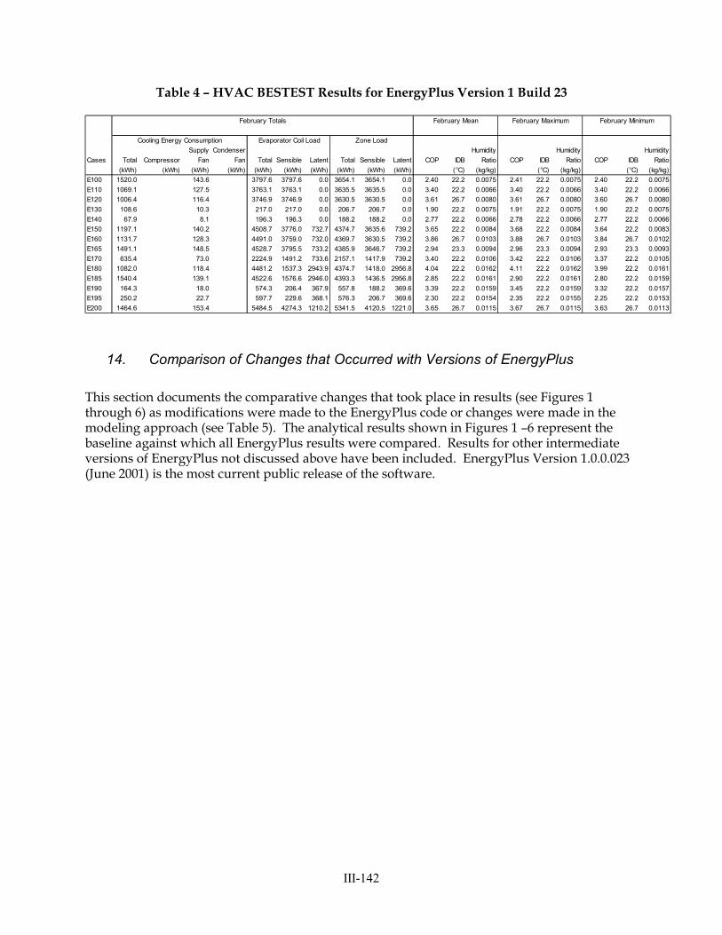
III-142

Table 4 – HVAC BESTEST Results for EnergyPlus Version 1 Build 23



February Mean February Maximum February Minimum


February Totals

14. Comparison of Changes that Occurred with Versions of EnergyPlus

This section documents the comparative changes that took place in results (see Figures 1through 6) as modifications were made to the EnergyPlus code or changes were made in themodeling approach (see Table 5). The analytical results shown in Figures 1 –6 represent thebaseline against which all EnergyPlus results were compared. Results for other intermediateversions of EnergyPlus not discussed above have been included. EnergyPlus Version 1.0.0.023(June 2001) is the most current public release of the software.

III-143

Table 5 – Summary of EnergyPlus Changes that were Implemented

Version Input File Changes Code ChangesBeta 5-12 thruBeta 5-

14

DX coil calculations modified to account for cyclingModified method of calculating SHR and coil bypass

factor

Beta 5-15 thruBeta 5-

18

Changed DX coil object names Changed name of DX coil object fromCOIL:DX:DOE2 to COIL:DX:BF-Empirical to betterrepresent its algorithmic basis(no impact on results)

Ver 1-01thru

Ver 1-11

Changed from blow-thru to draw-thru fanconfiguration

Changed to double precisionModified method of calculating coil outlet conditionsAdded draw-thru fan option to WindowAC model

Ver 1-12thru

Ver 1-14

New equipment performance curvesAdjusted fan mass flow and efficiency to

achieve desired mass flow and fan powerVer 1-15

thruVer 1-17

Went back to specified values for fan massflow and efficiency

Partial implementation of moist cpFan power calculated using a standard initial density

for volume to mass flow conversionVer 1-18

thruVer 1-19

Changed basis of CDF curve from net to grossOpened up min/max limits for performance

curves

Complete implementation of moist cphfg calculation modified for latent loads

Ver 1-20thru

Ver 1-23

Went back to original CDF curve (modifiedcurve used with Ver 1-19 was incorrect)

Changed fromFAN:SIMPLE:CONSTVOLUME toFAN:SIMPLE:ONOFF

Used CDF curve for fan power to account forcycling

Implemented optional PLR curve for fan cyclingChanged moisture initializations to use outdoor

humidity ratio

III-144

IEA HVAC BESTEST ComparisonIndoor Fan Electricity Consumption

E-Plus Output Variable: Fan Power[W]

-

20

40

60

80

100

120

140

160

180

E100 E110 E120 E130 E140 E150 E160 E165 E170 E180 E185 E190 E195 E200

HVAC BESTEST Case

Elec

tric

ity U

se (k

Wh)

Analytical/TUD

Analytical/HTAL1

Analytical/HTAL2

EnergyPlus Beta 5-07



EnergyPlus Ver 1-11

EnergyPlus Ver 1-14

EnergyPlus Ver 1-17

EnergyPlus Ver 1-19

EnergyPlus Ver 1-23

Figure 1 Indoor Fan Power Results for Versions of EnergyPlus

IEA HVAC BESTEST ComparisonDX Coil Electricity Consumption(includes Compressor + OD Fan)

E-Plus Output Variable: DX Coil Elec Power Cons[W]

-

200

400

600

800

1,000

1,200

1,400

1,600

E100 E110 E120 E130 E140 E150 E160 E165 E170 E180 E185 E190 E195 E200

HVAC BESTEST Case

Elec

tric

ity U

se (k

Wh)

Analytical/TUD

Analytical/HTAL1

Analytical/HTAL2




EnergyPlus Ver 1-11

EnergyPlus Ver 1-14

EnergyPlus Ver 1-17

EnergyPlus Ver 1-19

EnergyPlus Ver 1-23

Figure 2 Compressor Plus Outdoor Fan Electricity Consumption Results for Versions ofEnergyPlus

III-145

IEA HVAC BESTEST ComparisonTotal Cooling Coil Load

E-Plus Output Variable: (DX Coil Tot Cooling Energy[J])/3600/1000

-

1,000

2,000

3,000

4,000

5,000

6,000

7,000

E100 E110 E120 E130 E140 E150 E160 E165 E170 E180 E185 E190 E195 E200

HVAC BESTEST Case

Coo

ling

Coi

l Loa

d (k

Wh)

Analytical/TUD

Analytical/HTAL1

Analytical/HTAL2




EnergyPlus Ver 1-11

EnergyPlus Ver 1-14

EnergyPlus Ver 1-17

EnergyPlus Ver 1-19

EnergyPlus Ver 1-23

Figure 3 Total Cooling Coil Load Results for Versions of EnergyPlus

IEA HVAC BESTEST ComparisonCoefficient of Performance

E-Plus Output Variables: (Zone/Sys Sensible Cooling Energy[J] + Zone-Total Latent Gain[J])/3600/ Window AC Elec Power Cons[W]

0.00

0.50

1.00

1.50

2.00

2.50

3.00

3.50

4.00

4.50

E100 E110 E120 E130 E140 E150 E160 E165 E170 E180 E185 E190 E195 E200

HVAC BESTEST Case

Coe

ffici

ent o

f Per

form

ance

(CO

P)

Analytical/TUD

Analytical/HTAL1

Analytical/HTAL2




EnergyPlus Ver 1-11

EnergyPlus Ver 1-14

EnergyPlus Ver 1-17

EnergyPlus Ver 1-19

EnergyPlus Ver 1-23

Figure 4 Coefficient of Performance Results for Versions of EnergyPlus

III-146

IEA HVAC BESTEST ComparisonMean Indoor Drybulb Temperature

E-Plus Output Variable: Mean Air Temperature[C]

0.0

5.0

10.0

15.0

20.0

25.0

30.0

E100 E110 E120 E130 E140 E150 E160 E165 E170 E180 E185 E190 E195 E200

HVAC BESTEST Case

Indo

or D

rybu

lb T

empe

ratu

re (C

)

Analytical/TUD

Analytical/HTAL1

Analytical/HTAL2




EnergyPlus Ver 1-11

EnergyPlus Ver 1-14

EnergyPlus Ver 1-17

EnergyPlus Ver 1-19

EnergyPlus Ver 1-23

Figure 5 Indoor Dry-Bulb Temperature for Versions of EnergyPlus

IEA HVAC BESTEST ComparisonMean Indoor Humidity Ratio

E-Plus Output Variable: Zone Air Humidity Ratio[kg/kg]

0.0000

0.0020

0.0040

0.0060

0.0080

0.0100

0.0120

0.0140

0.0160

0.0180

E100 E110 E120 E130 E140 E150 E160 E165 E170 E180 E185 E190 E195 E200

HVAC BESTEST Case

Indo

or H

umid

ity R

atio

(kg/

kg)

Analytical/TUD

Analytical/HTAL1

Analytical/HTAL2




EnergyPlus Ver 1-11

EnergyPlus Ver 1-14

EnergyPlus Ver 1-17

EnergyPlus Ver 1-19

EnergyPlus Ver 1-23

Figure 6 Indoor Humidity Ratio Results for Versions of EnergyPlus

III-147

15. Conclusions

The HVAC BESTEST suite is a very valuable testing tool which provides excellent benchmarksfor testing HVAC system and equipment algorithms versus the results of other internationalbuilding simulation programs. As discussed above, HVAC BESTEST allowed the developers ofEnergyPlus to identify errors in algorithms and improve simulation accuracy.

16. References

ASHRAE 2001. ASHRAE Standard 140, Standard Method of Test for the Evaluation of BuildingEnergy Analysis Computer Programs, (expected publication date August 2001).

Crawley, Drury B, Linda K. Lawrie, Curtis O. Pedersen, and Frederick C. Winkelmann. 2000.“EnergyPlus: Energy Simulation Program,” in ASHRAE Journal, Vol. 42, No. 4 (April), pp.49-56.

Crawley, D. B., L. K. Lawrie, F. C. Winkelmann, W. F. Buhl, A. E. Erdem, C. O. Pedersen, R. J.Liesen, and D. E. Fisher. 1997. “The Next-Generation in Building Energy Simulation—AGlimpse of the Future,” in Proceedings of Building Simulation ‘97, Volume II, pp. 395-402,September 1997, Prague, Czech Republic, IBPSA.

Fisher, Daniel E, Russell D. Taylor, Fred Buhl, Richard J Liesen, and Richard K Strand. 1999. “A Modular, Loop-Based Approach to HVAC Energy Simulation And Its Implementationin EnergyPlus,” in Proceedings of Building Simulation ’99, September 1999, Kyoto, Japan,IBPSA.

Huang, Joe, Fred Winkelmann, Fred Buhl, Curtis Pedersen, Daniel Fisher, Richard Liesen,Russell Taylor, Richard Strand, Drury Crawley, and Linda Lawrie. 1999. “Linking theCOMIS Multi-Zone Airflow Model With the EnergyPlus Building Energy SimulationProgram,” in Proceedings of Building Simulation’99, September 1999, Kyoto, Japan, IBPSA.

Judkoff, R. and J. Neymark. (1995). International Energy Agency Building Energy Simulation Test(BESTEST) and Diagnostic Method. NREL/TP-472-6231. Golden, CO: National RenewableEnergy Laboratory.

Spitler, J. D., Rees, S. J., and X. Dongyi. 2001. Development of an Analytical Verification Test Suitefor Whole Building Energy Simulation Programs – Building Fabric, 1052RP Draft Final Report,December 2000.

Strand, Richard, Fred Winkelmann, Fred Buhl, Joe Huang, Richard Liesen, Curtis Pedersen,Daniel Fisher, Russell Taylor, Drury Crawley, and Linda Lawrie. 1999. “Enhancing andExtending the Capabilities of the Building Heat Balance Simulation Technique for use inEnergyPlus,” in Proceedings of Building Simulation ’99, September 1999, Kyoto, Japan, IBPSA.

Taylor, R. D, C. E. Pedersen, and L. K. Lawrie. 1990. "Simultaneous Simulation of Buildingsand Mechanical Systems in Heat Balance Based Energy Analysis Programs," in Proceedingsof the 3rd International Conference on System Simulation in Buildings, December 1990, Liege,Belgium.

III-148

Taylor R. D., C. E. Pedersen, D. E. Fisher, R. J. Liesen, and L. K. Lawrie. 1991. "Impact ofSimultaneous Simulation of Building and Mechanical Systems in Heat Balance BasedEnergy Analysis Programs on System Response and Control," in Proceedings of BuildingSimulation '91, August 1991, Nice, France, IBPSA.

Witte, M. J., Henninger, R.H., Glazer, J., and D. B. Crawley. 2001. "Testing and Validation of aNew Building Energy Simulation Program," Proceedings of Building Simulation 2001, to bepublished in August 2001, Rio de Janeiro, Brazil, International Building PerformanceSimulation Association (IBPSA).

http://www.eren.doe.gov/buildings/energy_tools/energyplus/

http://www.eren.doe.gov/buildings/energy_tools/energyplus/

III-149

Program name (please include version number)EnergyPlus Version 1.0.0.023

Your name, organisation, and countryMichael J. Witte, GARD Analytics, Inc., United States

Program status

Public domain

Commercial:

Research

x Other (please specify): Government-sponsored, end-user license is no charge, other license types have feesassociated with them

Solution method for unitary space cooling equipmentx Overall Performance Maps





x Both are calculated during the same timestep



Time stepFixed within code (please specify time step):

x User-specified (please specify time step): one hour for envelope

x Other (please specify): program automatically adjusts HVAC time step, <= envelope time step

Timing convention for meteorological data : sampling intervalFixed within code (please specify interval):

x User-specified: one hour

Timing convention for meteorological data : period covered by first recordx Fixed within code (please specify period or time which meteorological record covers): 0:00 - 1:00

User-specified

Meteorological data reconstitution schemeClimate assumed stepwise constant over sampling interval



III-150

Output timing conventionsProduces spot predictions at the end of each time step


x Produces average outputs for each hour (please specify period to which value relates): user-specified,hourly data is average or sum for previous hour, can specify output at each time step


Stratified model


Full CFD model


Zone air initial conditionsx Same as outside air


Internal gains output characteristicsPurely convective


x Radiative/Convective split specified by user: 100% convective for these tests




a Radiative/Convective split specified by user: for types of equipment not used in these tests


Control temperaturex Air temperature






III-151

Control propertiesx Ideal control as specified in the user's manual




Proportional control






Performance Map: independent variablesEntering Drybulb Temperature: program calculates adjustments internally



x Part Load Ratio

a Indoor Fan Air Flow Rate: always=1, because fan always operates at rated conditions



x Total Capacity

Sensible Capacity: program calculates internally based on user-specified nominal SHR

Bypass Factor: program calculates internally based on nominal SHR and current conditions

x Other (please specify): indoor fan power (function of PLR)

Performance Map: available curve fit techniquesx Linear, f(one independent variable): flow fraction curves set to constant=1

x Quadratic, f(one independent variable) : PLF-FPLR (cycling loss)

a Cubic, f(one independent variable):


x Bi-Quadratic, f(two independent variables): CAP-FT, EIR-FT


III-152

Performance Map: extrapolation limitsx Limits independent variables: 27.4 <= ODB <=48.1; 13.0 <= EWB <= 23.7, 0.0 <= PLR <= 1.0


No extrapolation limits





x Bypass factor model with ADP calculated from extending condition line: nominal BF is calculated from user-specified nominal SHR

x Fan heat included


Disaggregation of fans' electricity use directly in the simulation and outputx Indoor fan only

Outdoor fan only

Both indoor and outdoor fans disaggregated in the output


Economizer settings available (for E400 series)a Temperature (E400 series not run)

a Enthalpy (E400 series not run)

a Compressor Lockout (E400 series not run)


PART IV:

Simulation FieldTrial Results

IV-1

4.0 Part IV: Simulation Field Trial ResultsIntroductionHere we present the simulation results for the field trials of cases E100–E200. This results set is the finalversion after numerous iterations to incorporate clarifications to the test specification, simulation input deckcorrections, and simulation software improvements. An electronic version of the final results is included onthe accompanying CD in the file RESULTS.XLS, with its navigation instructions included inRESULTS.DOC. The results are presented here in the following order:

• Text summarizing the results organized by graph titles

• Graphs of results (beginning on p. IV-9)

• Tables of results (beginning on p. IV-23).

Table 4-1 summarizes the following information for the 11 models that were implemented by the sevenorganizations that participated in this project: model-authoring organization, model testing organization(“Implemented By”), and abbreviation labels used in the results tables, graphs, and the following text.

Except for the PROMETHEUS results, these results have been updated to be consistent with all testspecification revisions through May 2000. The PROMETHEUS participants (KST) were not able to workon this project after January 2000; therefore, they were unable to complete the refinement of theirsimulation results.

Independent simulations of the same program by separate organizations (such as has occurred with DOE-2.1E) minimized the potential for user errors for those simulations.

The text summarizes remaining disagreements of the simulations versus the analytical solutions observedin reviewing the data. Most of the discrepancies seen in previous results sets have been addressed (seePart III). However, a few disagreements remain.

Examples of Shorthand Language Used in the GraphsCase descriptions are summarized in Tables 1-1a and 1-1b (see Part 1). We have attempted to give a briefdescription of the cases in the x-axis labels of the accompanying graphs. The resulting shorthand languagefor these labels work according to the following examples; see Section 3.7 of Part III for definition ofacronyms.

“E110 as100 lo ODB” means the data being shown is for case E110 and case E110 is exactly like caseE100 except the ODB (outdoor dry-bulb temperature) was reduced. Similarly for the sensitivity plots,“E165-E160 IDB+ODB @hiSH” means the data shown are for the difference between cases E165 andE160, and this difference tests sensitivity to a variation in both IDB and ODB occurring at a high sensibleheat ratio.

Zone Condition and Input ChecksThese are organized sequentially according to the bar charts beginning on p. IV-9.

Mean IDBAll results are within 0.2°C of the setpoint except for TRNSYS-real for cases E100 – E165, E190 (within0.3°C–0.6°C, for realistic controller).

(Max-Min)/Mean IDBTRNSYS-real gives a variation ranging from 2% to 8%.

IV-2

Table 4-1. Participating Organizations and Computer Programs

Model Authoring Organization Implemented By Abbreviation

Analytical solution Hochschule Technik &Architektur Luzern, Switzerland(HTAL)

Hochschule Technik &Architektur Luzern,Switzerland

HTAL1

Analytical solutionwith realisticcontroller model

Hochschule Technik &Architektur Luzern, Switzerland

Hochschule Technik &Architektur Luzern,Switzerland

HTAL2

Analytical Solution Technische Universität Dresden,Germany (TUD)

Technische UniversitätDresden, Germany

TUD

CA-SIS V1 Electricité de France, France(EDF)

Electricité de France,France

CA-SIS

CLIM2000 2.1.6 Electricité de France, France Electricité de France,France

CLM2000

DOE-2.1E-088 LANL/LBNL/ESTSC,a,b,c USA CIEMAT,d Spain DOE21E/CIEMAT

DOE-2.1E-133 LANL/LBNL/JJH,a,b,e USA NREL/JNA,f USA DOE21E/NREL

ENERGYPLUS1.0.0.023

LBNL/UIUC/CERL/OSU/GARDAnalytics/FSEC/DOE-OBT,a,g,h,i,j,k

GARD Analytics, USA Energy+

PROMETHEUS Klimasystemtechnik, Germany(KST)

Klimasystemtechnik,Germany

Prometh

TRNSYS 14.2-TUD with idealcontroller model

University of Wisconsin, USA;Technische Universität Dresden,Ger.


TRN-idTRNSYS-ideal

TRNSYS 14.2-TUD with realcontroller model

University of Wisconsin, USA;Technische Universität Dresden,Ger.


TRN-reTRNSYS-real

aLANL: Los Alamos National LaboratorybLBNL: Lawrence Berkeley National LaboratorycESTSC: Energy Science and Technology Software Center (at Oak Ridge National Laboratory, USA)dCIEMAT: Centro de Investigaciones Energeticas, Medioambientales y TecnologicaseJJH: James J. Hirsch & AssociatesfNREL/JNA: National Renewable Energy Laboratory/J. Neymark & AssociatesgUIUC: University of Illinois Urbana/ChampaignhCERL: U.S. Army Corps of Engineers, Construction Engineering Research LaboratoriesiOSU: Oklahoma State UniversityjFSEC: University of Central Florida, Florida Solar Energy CenterkDOE-OBT: U.S. Department of Energy, Office of Building Technology, State and Community Programs, Energy Efficiency andRenewable Energy

IV-3

Mean Indoor Humidity RatioRange of the simulations’ disagreement with the analytical solutions:

• Wet coils indicate about 0%–9% range of disagreement.

• Dry coils indicate about 0%–3% range of disagreement.

• CLIM2000 has outlying value by 11% for E120 and 6% for E185 and E195.

The greatest disagreement appears to be in case E120 for CLIM2000, and PROMETHEUS. Because CA-SIS previously had a similar error and fixed it by improving their interpolation method, CLIM2000 andPROMETHEUS should be checked.

(Max-Min)/Mean Humidity RatioGenerally steady:

• CLIM2000 has 2% variation for dry coils

• CASIS, DOE21E/NREL, ENERGYPLUS, and PROMETHEUS vary 1%–2% for wet coils

• TRNSYS-real has up to 4% variation (E180).

Total Zone LoadZone loads mostly agree very closely for this near-adiabatic test cell with only internal gains. Differencesthat should be checked include:

• CLIM2000 is 1% below the mean for E200.

• PROMETHEUS' total zone load varies by 2% from the other results for cases E185 and E195(see sensible zone load below).

Sensible Zone LoadCLIM2000 is 1% below the mean for E200.

Results are similar to total zone load. However, PROMETHEUS’ sensible zone load varies from otherresults by 8% in E185 and 7% in E195—this difference should be investigated.

Latent Zone LoadNo substantial disagreements (all results well within 1%). PROMETHEUS has very slight (0.5%)disagreement with the analytical solutions. That disagreement may be related to the sensible zone loaddisagreement.

Output ComparisonsThese are organized sequentially according to the bar charts beginning on p. IV-13.

Mean Coefficient of Performance (COP)The greatest variation appears to be for dry-coil cases E100, E110, E130, and E140. These cases indicateabout 3%–10% variation between the minimum and maximum simulation results; PROMETHEUS

IV-4

generally has the greatest disagreement with the analytical verification results, with the greatestdisagreement seen at low part load ratio (PLR).

Notable disagreements:

• For low PLR cases, DOE21E/CIEMAT has 5%–6% disagreement for dry coils (E130 and E140)and 3% disagreement for wet coils (E190 and E195). This is because their COP calculation obtainsnet refrigeration effect from total coil load less fan energy (as noted later, the fan energy and “fanheat” are not consistent in DOE-2.1E); a different (and better agreeing) result is obtained if netrefrigeration effect is calculated from summing sensible and latent zone loads (as NREL did). Thisis further discussed in the modeler reports by NREL and CIEMAT (see Part III).

• PROMETHEUS E180–E195 ( cases with high latent internal gains) have generally higher COPthan the other results.

(Max-Mean)/Mean COPThe TRNSYS-real transient variation increases to up to 20% as PLR decreases (caused by the realisticcontroller).

Mean COP SensitivitiesDisagreements:

• PROMETHEUS has a number of disagreements where sensitivity is greater than the others (up to0.34 COP or 10%): e.g., E190–E140, E120–110, etc. These should be checked.

• Disagreements between NREL and CIEMAT's DOE-2.1E results (e.g., E180–E150) could berelated to the latent load discrepancy for NREL’s results as discussed in NREL’s and CIEMAT’smodeler reports (see Part III).

Total Space Cooling Electricity ConsumptionDisagreements:

• DOE21E/NREL results are 3% low in E170; half this difference was because COP DegradationFactor as a function of PLR (CDF f(PLR)) was not applied to indoor (ID) fan electricity.

• PROMETHEUS appears 5% low in E180.

Total Space Cooling Electricity SensitivitiesDisagreements are generally consistent with the COP sensitivity disagreements.

Compressor Electricity Consumption• These results are consistent with the total electric consumption results.

• Disaggregated results for compressor electric consumption were not provided for ENERGYPLUS.

Compressor Electricity Sensitivities• These results are consistent with the total electric consumption sensitivity results.

• Disaggregated results for compressor electric consumption were not provided for ENERGYPLUS.

IV-5

Indoor (Supply) Fan Electricity ConsumptionThe y-axis scale is smaller versus that for compressor consumption, so percentage differences are lesssignificant in terms of energy costs (for those cases where the fan cycled on/off with the compressor).However, the differences can still indicate disagreements that should be explained.

For DOE-2.1E results, the occurrence of relatively less indoor fan energy versus total energy compared tothe other results happens because in DOE-2.1E the disaggregated indoor fan does not pick up the COPdegradation factor (CDF) adjustment at part loads; the DOE2.1E/NREL compressor and outdoor fanresults do account for the CDF adjustment.

The sources of differences between CIEMAT and NREL DOE-2.1E simulations (e.g., in E110) shouldalso be isolated.

Indoor (Supply) Fan Electricity SensitivityThe differences in specific results among various cases for each simulation program are consistent with theindoor fan consumption results described above.

Outdoor (Condenser) Fan Electricity ConsumptionNote that the y-axis scale is again small, so percentage differences are less significant in terms of energycosts.

For E170 relative differences between compressor consumption versus outdoor (OD) fan consumption forDOE21E/CIEMAT results are not as consistent as for other results (compare “crowns” [tops] of graphs).This is because CDF was not applied to CIEMAT’s OD fan “hand” calculation in the DOE21E/CIEMATruns (see CIEMAT’s modeler report in Part III). Disaggregated results for compressor electricityconsumption were not provided for ENERGYPLUS.

Outdoor (Condenser) Fan Electricity SensitivitiesThe differences in specific results among various cases for each simulation program are consistent with theoutdoor fan consumption results described above. Disaggregated results for compressor electricityconsumption were not provided for ENERGYPLUS.

Total Coil LoadTotal coil loads exhibit generally good agreement. Notable loads differences are more apparent from theother loads charts described below.

Total Coil Load SensitivitiesTotal coil loads sensitivities exhibit generally good agreement. Notable loads differences are more apparentfrom the other loads charts described below.

Sensible Coil Load• DOE21E/NREL E180 and E185 seem slightly high; see below for “Sensible Coil Load Versus

Sensible Zone Load (Fan Heat).”

• PROMETHEUS seems slightly high in E185.

Sensible Coil Load SensitivitiesThe differences in specific results among various cases for each simulation program are consistent with thesensible coil load results described above.

Latent Coil LoadDOE21E/NREL, ENERGYPLUS, and PROMETHEUS are slightly low in E180 and E185.

IV-6

Latent Coil Load SensitivitiesThe differences in specific results among various cases for each simulation program are consistent with thesensible coil load results described above.

Sensible Coil Load Versus Sensible Zone Load (Fan Heat)The largest disagreements are:

• DOE21E/CIEMAT is high for E100-E120, E150-E165, E180, E185, and E200.

• DOE21E/NREL is high for E180, E185, and E200.

• PROMETHEUS is low for E170.

Latent Coil Load versus Latent Envelope LoadBecause there is no moisture diffusion for the envelope and the zone is at steady state, latent coil loadsshould match latent zone loads very closely.

Disagreements between latent coil and latent zone loads of >10 kWh occur for:

• DOE21E/NREL: E180, E185 (-30 kWh maximum difference)

• ENERGYPLUS: E180, E185, E200 (-13 kWh maximum difference).

Summary of Remaining Disagreements among the Simulation ProgramsComments about the final results of each simulation program are listed below. The disagreements arethose remaining after numerous iterations of simulations (including bug fixes and input corrections) andtest specification revisions. We have reported the remaining differences that did not have legitimatereasons to the appropriate code authors.

• CA-SIS/EDF

o The modeler report indicates that the performance map was revised (extrapolated) manuallyto run the cases. This makes it difficult for a typical CA-SIS user to obtain the same resultsas the EDF development group has obtained for these test cases. Extrapolation of the givenperformance data should be automated within CA-SIS.

• CLIM2000/EDF

o The indoor humidity ratios for E185 and E195 are outlying by 5%.

o The zone sensible and total loads are 1% below the mean for E200.

• DOE21E/CIEMAT

o The disaggregated indoor fan does not pick up the CDF adjustment.

o The OD fan energy does not appear to pick up the CDF adjustment.

o The difference between sensible coil load and sensible zone load (fan heat) is up to 37%higher throughout relative to this difference for the analytical solution results (this might bea bug in the software). This output magnifies an effect that does not appear to have muchimpact on the energy consumption for these test cases, but could be important for othersimulations.

• DOE21E/NREL

IV-7

o The disaggregated indoor fan does not pick up the CDF adjustment.

o The difference between the sensible coil and zone load (fan heat) is high in E180 and E185.

o The latent coil load is slightly (1%) different from the latent zone load in E180 and E185.

o The differences in results versus DOE21E/CIEMAT are attributable to differences betweenDOE-2.1E’s RESYS2 (used by NREL) and PTAC (used by CIEMAT) system models (e.g.,PTAC requires a blow-through ID fan), and because NREL and CIEMAT used differentversions (from different suppliers) of the software.

• ENERGYPLUS

o Latent coil load is slightly (<1%) different from latent zone load in wet-coil cases.

• PROMETHEUS/KST

KST was not able to complete refinement of their simulation results for this project because they couldnot participate in the task beyond January 2000.

o A number of COP sensitivity disagreements (E180–E150, E190–E140, E120–E110, etc)should be checked.

o Total electric consumption is 5% lower than the others in E180.

o The sensible zone load varies by 8% in E185 (7% in E195).

o The current results may not enable extrapolation.

o Performance map interpolation techniques for E120, and possible improper use of dry coilsensible capacity data (based on E120 humidity ratio result) should be checked.

o The fan heat is low in E170.

• TRNSYS-ideal/TUD

o No apparent disagreements.

• TRNSYS-real/TUD

o The following disagreements are acceptable and are caused by using a realistic controllermodel with 36-s (0.01-h) timesteps:

� Transient variations of IDB of 0.5°C to 2.1°C (except for E200)

� Mean IDB is 0.3°–0.6°C from set point in some cases

� Greater transient variations of COP than the other simulations. This does not causedisagreements for mean COP, consumption, and loads. Greatest transient variationis at low PLR.

Summary Ranges of Simulation Results DisagreementsAs shown in Table 4-2, the mean results of COP and total energy consumption for the programs are onaverage within <1% of the analytical solution results, with variations up to 2% for the low PLR dry coilcases (E130 and E140). Ranges of disagreement are further tabulated below. This summary excludes resultsfor PROMETHEUS; KST suspected error(s) in its software but was unable to correct them or complete thisproject.

IV-8

Table 4-2. Ranges of Disagreement versus Analytical Solutions

Cases Dry coil Wet coil

Energy 0%–6%a 0%–3%a

COP 0%–6%a 0%–3%a

Humidity Ratio 0%–11%a 0%–7%a

Zone Temperature 0.0°C–0.7°C(0.1°C)b

0.0°C–0.5°C(0.0°C–0.1°C)b

a % = (ABS(Sim - AnSoln))/AnSoln × 100%; sim = each simulation result, AnSoln = avg(TUD,HTAL1).b Excludes results for TRNSYS-TUD with realistic controller.

The higher level of disagreement in the dry-coil cases occurs for the case with lowest PLR and is related tosome potential problems that have been documented for DOE-2.1E (ESTSC version 088 and JJH version133) in both the CIEMAT and NREL results (see Part III). The larger disagreements for zone humidityratio are caused by disagreements for the CLIM2000 and DOE21E/CIEMAT results (CIEMAT used aPTAC, which only allows for a blow-through fan rather than the draw-through fan of the test specification).The disagreement in zone temperature results is primarily from the TRNSYS-TUD simulation results,where a realistic controller was applied on a short timestep (36 s); all other simulation results apply idealcontrol.

IV-9

HVAC BESTEST: Mean Indoor Drybulb Temperature

0

5

10

15

20

25

30

E100 d

ry lo

IDB hi

ODB

E110 a

s100

lo O

DB

E120 a

s100

hiID

B

E130 a

s100

lo PLR

E140 a

s130

lo O

DB

E150 a

s110

hiSHR

E160 a

s150

hiID

B

E165 a

s150

mID

B mODB

E170 a

s150

mSHR m

PLR

E180 a

s150

loSHR

E185 l

oSHR hi

ODB

E190 a

s180

loPLR

E195 a

s185

loPLR

E200 A

RI PLR

=1 hiSHR

Tem

pera

ture

(°C

)

CASIS/EDF CLIM2000/EDF DOE-2.1E/CIEMAT DOE-2.1E/NREL ENERGY+/GARD PROMETHEUS/KSTTRNSYS-ideal/TUD TRNSYS-real/TUD Analytical/TUD Analytical/HTAL1 Analytical/HTAL2

HVAC BESTEST: (Maximum - Minimum)/Mean Indoor Drybulb Temperature

0

0.01

0.02

0.03

0.04

0.05

0.06

0.07

0.08

0.09

E100 d

ry lo

IDB hi

ODB

E110 a

s100

lo O

DB

E120 a

s100

hiID

B

E130 a

s100

lo P

LR

E140 a

s130

lo O

DB

E150 a

s110

hiSHR

E160 a

s150

hiID

B

E165 a

s150

mID

B mODB

E170 a

s150

mSHR m

PLR

E180 a

s150

loSHR

E185 l

oSHR hi

ODB

E190 a

s180

loPLR

E195 a

s185

loPLR

E200 A

RI PLR

=1 hiSHR

Frac

tiona

l Var

iatio

n


IV-10

HVAC BESTEST: Mean Indoor Humidity Ratio

0

0.002

0.004

0.006

0.008

0.01

0.012

0.014

0.016

0.018

E100 d

ry lo

IDB hi

ODB

E110 a

s100

lo O

DB

E120 a

s100

hiID

B

E130 a

s100

lo PLR

E140 a

s130

lo O

DB

E150 a

s110

hiSHR

E160 a

s150

hiID

B

E165 a

s150

mID

B mODB

E170 a

s150

mSHR m

PLR

E180 a

s150

loSHR

E185 l

oSHR hi

ODB

E190 a

s180

loPLR

E195 a

s185

loPLR

E200 A

RI PLR

=1 hi

SHR

Hum

idity

Rat

io (k

g/kg

)


HVAC BESTEST: (Maximum - Minimum)/Mean Indoor Humidity Ratio

0

0.01

0.02

0.03

0.04

0.05

0.06

0.07

0.08

0.09

0.1

E100 d

ry lo

IDB hi

ODB

E110 a

s100

lo O

DB

E120 a

s100

hiID

B

E130 a

s100

lo PLR

E140 a

s130

lo O

DB

E150 a

s110

hiSHR

E160 a

s150

hiID

B

E165 a

s150

mID

B mODB

E170 a

s150

mSHR m

PLR

E180 a

s150

loSHR

E185 l

oSHR hi

ODB

E190 a

s180

loPLR

E195 a

s185

loPLR

E200 A

RI PLR

=1 hiSHR

Frac

tiona

l Var

iatio

n


IV-11

HVAC BESTEST: Total Zone Load

0

1000

2000

3000

4000

5000

6000

E100 d

ry lo

IDB hi

ODB

E110 a

s100

lo O

DB

E120 a

s100

hiID

B

E130 a

s100

lo P

LR

E140 a

s130

lo O

DB

E150 a

s110

hiSHR

E160 a

s150

hiID

B

E165 a

s150

mID

B mODB

E170 a

s150

mSHR m

PLR

E180 a

s150

loSHR

E185 l

oSHR hi

ODB

E190 a

s180

loPLR

E195 a

s185

loPLR

E200 A

RI PLR

=1 hi

SHR

Load

(Wh

ther

mal

)


HVAC BESTEST: Sensible Zone Load

0

500

1000

1500

2000

2500

3000

3500

4000

4500

E100 d

ry lo

IDB hi

ODB

E110 a

s100

lo O

DB

E120 a

s100

hiID

B

E130 a

s100

lo PLR

E140 a

s130

lo O

DB

E150 a

s110

hiSHR

E160 a

s150

hiID

B

E165 a

s150

mID

B mODB

E170 a

s150

mSHR m

PLR

E180 a

s150

loSHR

E185 l

oSHR hi

ODB

E190 a

s180

loPLR

E195 a

s185

loPLR

E200 A

RI PLR

=1 hi

SHR

Load

(Wh

ther

mal

)


IV-12

HVAC BESTEST: Latent Zone Load

0

500

1000

1500

2000

2500

3000

E100 d

ry lo

IDB hi

ODB

E110 a

s100

lo O

DB

E120 a

s100

hiID

B

E130 a

s100

lo PLR

E140 a

s130

lo O

DB

E150 a

s110

hiSHR

E160 a

s150

hiID

B

E165 a

s150

mID

B mODB

E170 a

s150

mSHR m

PLR

E180 a

s150

loSHR

E185 l

oSHR hi

ODB

E190 a

s180

loPLR

E195 a

s185

loPLR

E200 A

RI PLR

=1 hi

SHR

Load

(Wh

ther

mal

)


IV-13

HVAC BESTEST: Mean COP

0

0.5

1

1.5

2

2.5

3

3.5

4

4.5

E100 d

ry lo

IDB hi

ODB

E110 a

s100

lo O

DB

E120 a

s100

hiID

B

E130 a

s100

lo PLR

E140 a

s130

lo O

DB

E150 a

s110

hiSHR

E160 a

s150

hiID

B

E165 a

s150

mID

B mODB

E170 a

s150

mSHR m

PLR

E180 a

s150

loSHR

E185 l

oSHR hi

ODB

E190 a

s180

loPLR

E195 a

s185

loPLR

E200 A

RI PLR

=1 hiSHR

CO

P


HVAC BESTEST: (Maximum - Minimum)/Mean COP

0

0.05

0.1

0.15

0.2

0.25

E100 d

ry lo

IDB hi

ODB

E110 a

s100

lo O

DB

E120 a

s100

hiID

B

E130 a

s100

lo PLR

E140 a

s130

lo O

DB

E150 a

s110

hiSHR

E160 a

s150

hiID

B

E165 a

s150

mID

B mODB

E170 a

s150

mSHR m

PLR

E180 a

s150

loSHR

E185 l

oSHR hi

ODB

E190 a

s180

loPLR

E195 a

s185

loPLR

E200 A

RI PLR

=1 hi

SHR

Frac

tiona

l Var

iatio

n


IV-14

HVAC BESTEST: Mean COP Sensitivities

-1.5

-1

-0.5

0

0.5

1

1.5

E110-1

00 O

DB

E120-1

10 ID

B

E120-1

00 ID

B+ODB

E130-1

00 PLR

E140-1

30 O

DB @loP

LR

E140-1

10 PLR

@loO

DB

E150-1

10 hi

SHR v. dr

y

E160-1

50 ID

B @hiS

HR

E165-1

60 ID

B+ODB @

hiSH

E170-1

50 se

ns x

0.39

E180-1

50 SHR

E180-1

70 la

t x 4

E185-1

80 O

DB @loS

HR

E190-1

80 PLR

@loS

HR

E190-1

40 la

t @loP

LR

E195-1

90 O

DB @loP

LloSH

E195-1

85 PLR

@loS

HR

E195-1

30 la

t @loP

LR

E200-1

00 ARI v

dry

delta

CO

P


IV-15

HVAC BESTEST: Total Space Cooling Electricity Consumption

0

200

400

600

800

1000

1200

1400

1600

E100 d

ry lo

IDB hi

ODB

E110 a

s100

lo O

DB

E120 a

s100

hiID

B

E130 a

s100

lo PLR

E140 a

s130

lo O

DB

E150 a

s110

hiSHR

E160 a

s150

hiID

B

E165 a

s150

mID

B mODB

E170 a

s150

mSHR m

PLR

E180 a

s150

loSHR

E185 l

oSHR hi

ODB

E190 a

s180

loPLR

E195 a

s185

loPLR

E200 A

RI PLR

=1 hi

SHR

Elec

tric

ity C

onsu

mpt

ion

(kW

h)


HVAC BESTEST: Total Space Cooling Electricity Sensitivities

-1500

-1300

-1100

-900

-700

-500

-300

-100

100

300

500

E110-1

00 O

DB

E120-1

10 ID

B

E120-1

00 ID

B+ODB

E130-1

00 PLR

E140-1

30 O

DB @loP

LR

E140-1

10 PLR

@loO

DB

E150-1

10 hi

SHR v. dr

y

E160-1

50 ID

B @hiS

HR

E165-1

60 ID

B+ODB @

hiSH

E170-1

50 se

ns x

0.39

E180-1

50 SHR

E180-1

70 la

t x 4

E185-1

80 O

DB @loS

HR

E190-1

80 PLR

@loS

HR

E190-1

40 la

t @loP

LR

E195-1

90 O

DB @loP

LloSH

E195-1

85 PLR

@loS

HR

E195-1

30 la

t @loP

LR

E200-1

00 ARI v

dryde

lta E

lect

ricity

Con

sum

ptio

n (k

Wh)


IV-16

HVAC BESTEST: Compressor Electricity Consumption

0

200

400

600

800

1000

1200

1400

E100 d

ry lo

IDB hi

ODB

E110 a

s100

lo O

DB

E120 a

s100

hiID

B

E130 a

s100

lo PLR

E140 a

s130

lo O

DB

E150 a

s110

hiSHR

E160 a

s150

hiID

B

E165 a

s150

mID

B mODB

E170 a

s150

mSHR m

PLR

E180 a

s150

loSHR

E185 l

oSHR hi

ODB

E190 a

s180

loPLR

E195 a

s185

loPLR

E200 A

RI PLR

=1 hi

SHR

Elec

tric

ity C

onsu

mpt

ion

(kW

h)


HVAC BESTEST: Total Compressor Electricity Sensitivities

-1500

-1300

-1100

-900

-700

-500

-300

-100

100

300

500

E110-1

00 O

DB

E120-1

10 ID

B

E120-1

00 ID

B+ODB

E130-1

00 PLR

E140-1

30 O

DB @loP

LR

E140-1

10 P

LR @

loODB

E150-1

10 hi

SHR v. dr

y

E160-1

50 ID

B @hiS

HR

E165-1

60 ID

B+ODB @

hiSH

E170-1

50 se

ns x

0.39

E180-1

50 SHR

E180-1

70 la

t x 4

E185-1

80 O

DB @loS

HR

E190-1

80 PLR

@loS

HR

E190-1

40 la

t @loP

LR

E195-1

90 O

DB @loP

LloSH

E195-1

85 PLR

@loS

HR

E195-1

30 la

t @loP

LR

E200-1

00 ARI v

dryde

lta E

lect

ricity

Con

sum

ptio

n (k

Wh)


IV-17

HVAC BESTEST: Total Indoor (Supply) Fan Electricity Consumption

0

20

40

60

80

100

120

140

160

E100 d

ry lo

IDB hi

ODB

E110 a

s100

lo O

DB

E120 a

s100

hiID

B

E130 a

s100

lo P

LR

E140 a

s130

lo O

DB

E150 a

s110

hiSHR

E160 a

s150

hiID

B

E165 a

s150

mID

B mODB

E170 a

s150

mSHR m

PLR

E180 a

s150

loSHR

E185 l

oSHR hi

ODB

E190 a

s180

loPLR

E195 a

s185

loPLR

E200 A

RI PLR

=1 hi

SHR

Elec

tric

ity C

onsu

mpt

ion

(kW

h)


HVAC BESTEST: Indoor (Supply) Fan Electricity Sensitivities

-150

-100

-50

0

50

E110-1

00 O

DB

E120-1

10 ID

B

E120-1

00 ID

B+ODB

E130-1

00 PLR

E140-1

30 O

DB @loP

LR

E140-1

10 PLR

@loO

DB

E150-1

10 hi

SHR v. dr

y

E160-1

50 ID

B @hiS

HR

E165-1

60 ID

B+ODB @

hiSH

E170-1

50 se

ns x

0.39

E180-1

50 SHR

E180-1

70 la

t x 4

E185-1

80 O

DB @loS

HR

E190-1

80 PLR

@loS

HR

E190-1

40 la

t @loP

LR

E195-1

90 O

DB @loP

LloSH

E195-1

85 PLR

@loS

HR

E195-1

30 la

t @loP

LR

E200-1

00 ARI v

dryde

lta E

lect

ricity

Con

sum

ptio

n (k

Wh)


IV-18

HVAC BESTEST: Outdoor (Condenser) Fan Electricity Consumption

0

10

20

30

40

50

60

70

80

E100 d

ry lo

IDB hi

ODB

E110 a

s100

lo O

DB

E120 a

s100

hiID

B

E130 a

s100

lo PLR

E140 a

s130

lo O

DB

E150 a

s110

hiSHR

E160 a

s150

hiID

B

E165 a

s150

mID

B mODB

E170 a

s150

mSHR m

PLR

E180 a

s150

loSHR

E185 l

oSHR hi

ODB

E190 a

s180

loPLR

E195 a

s185

loPLR

E200 A

RI PLR

=1 hi

SHR

Elec

tric

ity C

onsu

mpt

ion

(kW

h)


HVAC BESTEST: Outdoor (Condenser) Fan Electricity Sensitivities

-80

-60

-40

-20

0

20

40

E110-1

00 O

DB

E120-1

10 ID

B

E120-1

00 ID

B+ODB

E130-1

00 PLR

E140-1

30 O

DB @loP

LR

E140-1

10 PLR

@loO

DB

E150-1

10 hi

SHR v. dr

y

E160-1

50 ID

B @hiS

HR

E165-1

60 ID

B+ODB @

hiSH

E170-1

50 se

ns x

0.39

E180-1

50 SHR

E180-1

70 la

t x 4

E185-1

80 O

DB @loS

HR

E190-1

80 PLR

@loS

HR

E190-1

40 la

t @loP

LR

E195-1

90 O

DB @loP

LloSH

E195-1

85 PLR

@loS

HR

E195-1

30 la

t @loP

LR

E200-1

00 ARI v

dryde

lta E

lect

ricity

Con

sum

ptio

n (k

Wh)


IV-19

HVAC BESTEST: Total Coil Load

0

1000

2000

3000

4000

5000

6000

E100 d

ry lo

IDB hi

ODB

E110 a

s100

lo O

DB

E120 a

s100

hiID

B

E130 a

s100

lo P

LR

E140 a

s130

lo O

DB

E150 a

s110

hiSHR

E160 a

s150

hiID

B

E165 a

s150

mID

B mODB

E170 a

s150

mSHR m

PLR

E180 a

s150

loSHR

E185 l

oSHR hi

ODB

E190 a

s180

loPLR

E195 a

s185

loPLR

E200 A

RI PLR

=1 hi

SHR

Load

(kW

h th

erm

al)


HVAC BESTEST: Total Coil Load Sensitivities

-5000

-4000

-3000

-2000

-1000

0

1000

2000

3000

E110-1

00 O

DB

E120-1

10 ID

B

E120-1

00 ID

B+ODB

E130-1

00 PLR

E140-1

30 O

DB @loP

LR

E140-1

10 PLR

@loO

DB

E150-1

10 hi

SHR v. dr

y

E160-1

50 ID

B @hiS

HR

E165-1

60 ID

B+ODB @

hiSH

E170-1

50 se

ns x

0.39

E180-1

50 SHR

E180-1

70 la

t x 4

E185-1

80 O

DB @loS

HR

E190-1

80 PLR

@loS

HR

E190-1

40 la

t @loP

LR

E195-1

90 O

DB @loP

LloSH

E195-1

85 PLR

@loS

HR

E195-1

30 la

t @loP

LR

E200-1

00 ARI v

dry

delta

Loa

d (k

Wh

ther

mal

)


IV-20

HVAC BESTEST: Sensible Coil Load Sensitivities

-4000

-3500

-3000

-2500

-2000

-1500

-1000

-500

0

500

1000

E110-1

00 O

DB

E120-1

10 ID

B

E120-1

00 ID

B+ODB

E130-1

00 PLR

E140-1

30 O

DB @loP

LR

E140-1

10 PLR

@loO

DB

E150-1

10 hi

SHR v. dr

y

E160-1

50 ID

B @hiS

HR

E165-1

60 ID

B+ODB @hiS

H

E170-1

50 se

ns x

0.39

E180-1

50 SHR

E180-1

70 la

t x 4

E185-1

80 O

DB @loS

HR

E190-1

80 PLR

@loS

HR

E190-1

40 la

t @loP

LR

E195-1

90 O

DB @loP

LloSH

E195-1

85 PLR

@loS

HR

E195-1

30 la

t @loP

LR

E200-1

00 ARI v

dry

delta

Loa

d (k

Wh

ther

mal

)


HVAC BESTEST: Sensible Coil Load

0

500

1000

1500

2000

2500

3000

3500

4000

4500

5000

E100 d

ry lo

IDB hi

ODB

E110 a

s100

lo O

DB

E120 a

s100

hiID

B

E130 a

s100

lo PLR

E140 a

s130

lo O

DB

E150 a

s110

hiSHR

E160 a

s150

hiID

B

E165 a

s150

mID

B mODB

E170 a

s150

mSHR m

PLR

E180 a

s150

loSHR

E185 l

oSHR hi

ODB

E190 a

s180

loPLR

E195 a

s185

loPLR

E200 A

RI PLR

=1 hiSHR

Load

(kW

h th

erm

al)


IV-21

HVAC BESTEST: Latent Coil Load Sensitivities

-3000

-2000

-1000

0

1000

2000

3000

E110-1

00 O

DB

E120-1

10 ID

B

E120-1

00 ID

B+ODB

E130-1

00 PLR

E140-1

30 O

DB @loP

LR

E140-1

10 PLR

@loO

DB

E150-1

10 hi

SHR v. dr

y

E160-1

50 ID

B @hiS

HR

E165-1

60 ID

B+ODB @hiS

H

E170-1

50 se

ns x

0.39

E180-1

50 SHR

E180-1

70 la

t x 4

E185-1

80 O

DB @loS

HR

E190-1

80 PLR

@loS

HR

E190-1

40 la

t @loP

LR

E195-1

90 O

DB @loP

LloSH

E195-1

85 PLR

@loS

HR

E195-1

30 la

t @loP

LR

E200-1

00 ARI v

dry

delta

Loa

d (k

Wh

ther

mal

)


HVAC BESTEST: Latent Coil Load

0

500

1000

1500

2000

2500

3000

3500

E100 d

ry lo

IDB hi

ODB

E110 a

s100

lo O

DB

E120 a

s100

hiID

B

E130 a

s100

lo PLR

E140 a

s130

lo O

DB

E150 a

s110

hiSHR

E160 a

s150

hiID

B

E165 a

s150

mID

B mODB

E170 a

s150

mSHR m

PLR

E180 a

s150

loSHR

E185 l

oSHR hi

ODB

E190 a

s180

loPLR

E195 a

s185

loPLR

E200 A

RI PLR

=1 hi

SHR

Load

(kW

h th

erm

al)


IV-22

HVAC BESTEST: Latent Coil Load - Latent Zone Load (Should = 0)

-35

-30

-25

-20

-15

-10

-5

0

5

E100 d

ry lo

IDB hi

ODB

E110 a

s100

lo O

DB

E120 a

s100

hiID

B

E130 a

s100

lo PLR

E140 a

s130

lo O

DB

E150 a

s110

hiSHR

E160 a

s150

hiID

B

E165 a

s150

mID

B mODB

E170 a

s150

mSHR m

PLR

E180 a

s150

loSHR

E185 l

oSHR hi

ODB

E190 a

s180

loPLR

E195 a

s185

loPLR

E200 A

RI PLR

=1 hi

SHR

Load

(kW

h th

erm

al)


HVAC BESTEST: Sensible Coil Load - Zone Load (Fan Heat)

0

50

100

150

200

250

E100 d

ry lo

IDB hi

ODB

E110 a

s100

lo O

DB

E120 a

s100

hiID

B

E130 a

s100

lo PLR

E140 a

s130

lo O

DB

E150 a

s110

hiSHR

E160 a

s150

hiID

B

E165 a

s150

mID

B mODB

E170 a

s150

mSHR m

PLR

E180 a

s150

loSHR

E185 l

oSHR hi

ODB

E190 a

s180

loPLR

E195 a

s185

loPLR

E200 A

RI PLR

=1 hi

SHR

Load

(kW

h th

erm

al)


IV-23

Space Cooling Electricity ConsumptionEnergy Consumption, Total (kWh,e) Stat ist ics, All Results

CA-SIS CLM2000 DOE21E DOE21E Energy+ Prometh TRN-id TRN-re (Max-Min) Analyt icalEDF EDF CIEMAT NREL GARD KST TUD TUD Min Max / Analyt ical TUD HTAL1 HTAL2

E100 1531 1530 1521 1519 1520 1584 1522 1512 1512 1584 4.7% 1531 1531 1531E110 1077 1089 1061 1065 1069 1130 1067 1062 1061 1130 6.3% 1076 1077 1077E120 1012 1012 1011 1003 1006 988 1007 1002 988 1012 2.4% 1013 1011 1011E130 110 109 105 106 109 114 109 110 105 114 7.5% 111 110 110E140 68 69 65 66 68 72 68 69 65 72 9.7% 69 69 68E150 1208 1207 1202 1183 1197 1215 1199 1192 1183 1215 2.7% 1206 1207 1207E160 1140 1139 1138 1107 1132 1158 1137 1133 1107 1158 4.5% 1140 1139 1139E165 1502 1501 1499 1470 1491 1493 1500 1490 1470 1502 2.1% 1498 1500 1500E170 638 638 629 620 635 616 636 636 616 638 3.4% 641 638 638E180 1083 1082 1077 1080 1082 1031 1081 1080 1031 1083 4.8% 1083 1082 1082E185 1544 1543 1541 1547 1540 1533 1542 1538 1533 1547 0.9% 1545 1543 1543E190 164 164 160 160 164 155 164 165 155 165 6.1% 165 164 164E195 250 250 245 246 250 245 250 252 245 252 2.8% 252 250 250E200 1477 1464 1468 1440 1465 1487 1480 1480 1440 1487 3.2% 1476 1477 1477Energy Consumption, Compressor (kWh,e) Stat ist ics, All Results


E100 1319 1318 1307 1311 1363 1311 1303 1303 1363 4.6% 1319 1319 1319E110 889 899 866 883 932 879 876 866 932 7.5% 888 889 889E120 840 840 850 838 819 836 832 819 850 3.6% 841 839 839E130 95 94 93 93 98 94 95 93 98 5.1% 95 94 94E140 57 57 55 56 59 56 57 55 59 7.7% 57 57 56E150 1000 999 1007 982 1007 992 987 982 1007 2.5% 999 999 999E160 950 949 963 926 965 947 944 926 965 4.1% 950 949 949E165 1283 1281 1291 1256 1275 1280 1272 1256 1291 2.8% 1279 1280 1280E170 531 530 539 523 513 528 529 513 539 4.9% 533 530 530E180 909 908 914 912 864 907 906 864 914 5.5% 908 908 908E185 1340 1339 1343 1344 1331 1337 1334 1331 1344 1.0% 1340 1339 1338E190 138 138 139 138 130 138 138 130 139 6.8% 138 138 138E195 217 217 219 217 212 216 218 212 219 3.1% 219 217 217E200 1250 1239 1249 1218 1260 1253 1253 1218 1260 3.3% 1249 1250 1250Energy Consumption, Supply Fan (kWh,e) Stat ist ics, All Results


E100 144 144 145 141 144 150 144 142 141 150 6.4% 144 144 144E110 128 129 133 122 128 134 128 127 122 134 9.6% 128 128 128E120 117 117 110 110 116 115 117 115 110 117 6.3% 117 117 117E130 10 10 8 8 10 11 10 10 8 11 26.9% 10 10 10E140 8 8 7 6 8 9 8 8 6 9 30.4% 8 8 8E150 141 141 133 136 140 142 141 139 133 142 6.4% 141 141 141E160 129 129 119 121 128 131 129 128 119 131 9.4% 129 129 129E165 149 150 142 145 149 149 149 148 142 150 5.6% 149 149 149E170 73 73 61 63 73 71 73 73 61 73 16.1% 74 73 73E180 118 119 111 112 118 113 118 118 111 119 6.9% 119 119 119E185 139 139 135 137 139 138 139 139 135 139 3.0% 139 139 139E190 18 18 14 14 18 17 18 18 14 18 22.8% 18 18 18E195 23 23 18 18 23 22 23 23 18 23 23.1% 23 23 23E200 154 153 149 151 153 155 155 155 149 155 3.9% 154 155 155Energy Consumption, Condenser Fan (kWh,e) Stat ist ics, All Results


E100 68 68 68 67 70 67 67 67 70 5.3% 68 68 68E110 60 61 62 60 63 60 59 59 63 5.9% 60 60 60E120 55 55 51 55 54 55 54 51 55 6.5% 55 55 55E130 5 5 4 5 5 5 5 4 5 24.5% 5 5 5E140 4 4 3 4 4 4 4 3 4 19.1% 4 4 4E150 66 66 62 65 67 66 65 62 67 6.3% 66 66 66E160 61 61 56 60 62 61 60 56 62 9.2% 61 61 61E165 70 70 67 69 70 70 69 67 70 5.2% 70 70 70E170 34 34 29 34 33 34 34 29 34 16.1% 35 34 34E180 56 56 52 56 53 56 55 52 56 7.1% 56 56 56E185 65 65 63 66 65 65 65 63 66 3.9% 65 65 65E190 8 9 7 8 8 8 9 7 9 27.6% 9 9 9E195 11 11 8 11 10 11 11 8 11 25.0% 11 11 11E200 73 72 70 71 73 73 73 70 73 4.1% 73 73 73

results .xls q:a06..q75; 07/16/01

IV-24

COP: Mean, and (Max-Min)/ MeanMean COP Statist ics, All Results


E100 2.39 2.39 2.43 2.41 2.40 2.31 2.40 2.42 2.31 2.43 5.0% 2.39 2.39 2.39E110 3.38 3.34 3.46 3.41 3.40 3.22 3.41 3.43 3.22 3.46 7.1% 3.38 3.38 3.38E120 3.59 3.59 3.61 3.62 3.61 3.68 3.61 3.63 3.59 3.68 2.5% 3.59 3.59 3.59E130 1.91 1.91 1.98 1.95 1.90 1.84 1.92 1.92 1.84 1.98 7.2% 1.89 1.91 1.91E140 2.77 2.73 2.92 2.85 2.77 2.65 2.80 2.80 2.65 2.92 9.6% 2.75 2.77 2.77E150 3.62 3.63 3.67 3.70 3.65 3.61 3.65 3.67 3.61 3.70 2.5% 3.63 3.63 3.63E160 3.84 3.84 3.87 3.95 3.86 3.78 3.85 3.86 3.78 3.95 4.4% 3.83 3.84 3.84E165 2.92 2.92 2.95 2.99 2.94 2.95 2.93 2.94 2.92 2.99 2.2% 2.93 2.93 2.93E170 3.38 3.39 3.44 3.48 3.40 3.52 3.39 3.40 3.38 3.52 4.2% 3.37 3.39 3.39E180 4.04 4.04 4.08 4.03 4.04 4.27 4.05 4.06 4.03 4.27 6.0% 4.04 4.04 4.04E185 2.85 2.85 2.87 2.82 2.85 2.92 2.85 2.86 2.82 2.92 3.4% 2.85 2.85 2.85E190 3.41 3.41 3.49 3.46 3.39 3.63 3.41 3.40 3.39 3.63 7.0% 3.39 3.41 3.41E195 2.31 2.31 2.36 2.34 2.30 2.41 2.32 2.31 2.30 2.41 4.7% 2.29 2.31 2.31E200 3.62 3.61 3.67 3.71 3.65 3.61 3.61 3.61 3.61 3.71 2.7% 3.62 3.62 3.62(Max - Min)/ Mean COP Statist ics, All Results


E100 0.000 0.001 0.002 0.001 0.003 0.009 0.000 0.000 0.000 0.009 0.000 0.000 0.000E110 0.000 0.010 0.002 0.001 0.003 0.006 0.000 0.011 0.000 0.011 0.000 0.000 0.000E120 0.000 0.004 0.001 0.001 0.003 0.008 0.000 0.012 0.000 0.012 0.000 0.000 0.000E130 0.000 0.038 0.013 0.009 0.004 0.011 0.000 0.172 0.000 0.172 0.000 0.000 0.000E140 0.000 0.056 0.011 0.019 0.004 0.008 0.000 0.204 0.000 0.204 0.000 0.000 0.000E150 0.003 0.003 0.001 0.005 0.011 0.006 0.000 0.009 0.000 0.011 0.000 0.000 0.001E160 0.003 0.005 0.001 0.003 0.011 0.008 0.000 0.010 0.000 0.011 0.000 0.000 0.000E165 0.010 0.003 0.001 0.003 0.012 0.007 0.000 0.008 0.000 0.012 0.000 0.000 0.000E170 0.000 0.006 0.002 0.004 0.015 0.006 0.000 0.043 0.000 0.043 0.000 0.000 0.000E180 0.005 0.002 0.002 0.010 0.029 0.014 0.000 0.012 0.000 0.029 0.000 0.000 0.000E185 0.007 0.004 0.002 0.010 0.034 0.014 0.000 0.009 0.000 0.034 0.000 0.000 0.000E190 0.000 0.023 0.007 0.019 0.040 0.025 0.000 0.101 0.000 0.101 0.000 0.000 0.000E195 0.000 0.017 0.008 0.017 0.043 0.021 0.000 0.086 0.000 0.086 0.000 0.000 0.000E200 0.006 0.000 0.000 0.005 0.012 0.006 0.000 0.000 0.000 0.012 0.000 0.000 0.000

results .xls q:a185..q220; 07/16/01

IV-25

Coil Loads: Total, Sensible, and LatentCoil Load, Total (kWh,thermal) Statist ics, All Results

CA-SIS CLM2000 DOE21E DOE21E Energy+ Prometh TRN-id TRN-re (Max-Min) Analyt icalEDF EDF CIEMAT NREL GARD KST TUD TUD Min Max / Analytical TUD HTAL1 HTAL2

E100 3800 3800 3841 3794 3798 3804 3800 3798 3794 3841 1.3% 3800 3800 3800E110 3765 3766 3804 3756 3763 3765 3765 3763 3756 3804 1.3% 3765 3765 3765E120 3749 3749 3763 3739 3747 3740 3748 3747 3739 3763 0.6% 3749 3749 3749E130 219 219 216 215 217 218 219 220 215 220 2.1% 219 219 219E140 198 198 196 195 196 197 198 199 195 199 2.0% 198 198 197E150 4517 4517 4543 4528 4509 4527 4517 4515 4509 4543 0.8% 4518 4517 4518E160 4501 4500 4516 4508 4491 4506 4500 4499 4491 4516 0.6% 4501 4500 4500E165 4538 4538 4567 4549 4529 4556 4537 4535 4529 4567 0.9% 4537 4537 4538E170 2233 2232 2226 2237 2225 2230 2232 2232 2225 2237 0.5% 2232 2232 2233E180 4495 4495 4510 4535 4481 4507 4495 4494 4481 4535 1.2% 4495 4495 4494E185 4507 4535 4565 4583 4523 4611 4535 4534 4507 4611 2.3% 4535 4535 4534E190 578 577 573 579 574 576 577 578 573 579 1.0% 578 577 578E195 602 601 595 602 598 607 601 601 595 607 1.9% 601 601 601E200 5498 5436 5534 5522 5484 5522 5498 5498 5436 5534 1.8% 5498 5498 5498Coil Load, Sensible (kWh,thermal) Statist ics, All Results


E100 3800 3800 3841 3794 3798 3804 3800 3798 3794 3841 1.3% 3800 3800 3800E110 3765 3766 3804 3756 3763 3765 3765 3763 3756 3804 1.3% 3765 3765 3765E120 3749 3749 3763 3739 3747 3740 3748 3747 3739 3763 0.6% 3749 3749 3749E130 219 219 216 215 217 218 219 220 215 220 2.1% 219 219 219E140 198 198 196 195 196 197 198 199 195 199 2.0% 198 198 197E150 3778 3778 3804 3786 3776 3788 3778 3776 3776 3804 0.7% 3778 3778 3779E160 3761 3761 3777 3769 3759 3766 3761 3760 3759 3777 0.5% 3761 3761 3761E165 3798 3798 3828 3809 3795 3817 3798 3796 3795 3828 0.9% 3798 3798 3799E170 1493 1493 1487 1498 1491 1493 1492 1492 1487 1498 0.7% 1493 1493 1493E180 1537 1538 1553 1607 1537 1563 1538 1537 1537 1607 4.5% 1538 1538 1538E185 1548 1578 1608 1653 1577 1665 1578 1577 1548 1665 7.4% 1578 1578 1578E190 208 208 203 212 206 208 208 208 203 212 4.4% 208 208 208E195 232 232 226 235 230 239 231 232 226 239 5.6% 232 232 232E200 4276 4215 4313 4303 4274 4300 4277 4277 4215 4313 2.3% 4277 4277 4277Coil Load, Latent (kWh,thermal) Statist ics, All Results


E100 0 0 0 0 0 0 0 0 0 0 0 0 0E110 0 0 0 0 0 0 0 0 0 0 0 0 0E120 0 0 0 0 0 0 0 0 0 0 0 0 0E130 0 0 0 0 0 0 0 0 0 0 0 0 0E140 0 0 0 0 0 0 0 0 0 0 0 0 0E150 739 739 739 742 733 739 739 739 733 742 1.2% 739 739 739E160 740 739 739 739 732 739 739 739 732 740 1.1% 739 739 739E165 740 739 739 740 733 739 739 739 733 740 1.0% 739 739 739E170 740 739 739 739 734 738 739 739 734 740 0.9% 739 739 739E180 2958 2957 2957 2928 2944 2943 2957 2957 2928 2958 1.0% 2957 2957 2956E185 2959 2957 2957 2930 2946 2946 2957 2957 2930 2959 1.0% 2958 2957 2956E190 370 370 370 366 368 368 370 370 366 370 1.0% 370 370 370E195 370 370 370 367 368 368 370 370 367 370 0.9% 370 370 370E200 1222 1221 1221 1219 1210 1222 1221 1221 1210 1222 1.0% 1221 1221 1221

results .xls q:bd77..bt147; 07/16/01Sensible Coil - Zone Load, (Fan Heat) (kWh,thermal) Statist ics, All Results


E100 144 144 187 139 144 148 144 142 139 187 33.6% 144 144 144E110 128 129 168 119 128 127 128 127 119 168 38.2% 128 128 128E120 117 117 133 108 116 107 117 115 107 133 22.1% 117 117 117E130 10 10 8 8 10 8 10 10 8 10 26.7% 10 10 10E140 8 8 7 6 8 7 8 8 6 8 25.0% 8 8 8E150 141 141 168 149 140 138 141 139 138 168 21.3% 141 141 142E160 129 129 147 137 129 125 129 128 125 147 16.9% 129 129 129E165 149 149 181 161 149 147 149 148 147 181 23.0% 149 149 150E170 73 73 69 79 73 61 73 73 61 79 24.5% 74 73 74E180 117 118 135 188 119 106 118 118 106 188 69.2% 118 119 118E185 109 139 171 215 140 134 139 139 109 215 76.6% 139 139 139E190 18 18 15 24 18 14 18 18 14 24 56.1% 18 18 18E195 23 23 18 28 23 18 23 23 18 28 43.8% 23 23 23E200 154 153 193 181 154 155 155 155 153 193 25.7% 154 155 155

IV-26

Zone Loads: Total, Sensible, and LatentZone Load, Total (kWh,thermal) Statistics, All Results

CA-SIS CLM2000 DOE21E DOE21E Energy+ Prometh TRN-id TRN-re (Max-Min) AnalyticalEDF EDF CIEMAT NREL GARD KST TUD TUD Min Max /Analytical TUD HTAL1 HTAL2

E100 3656 3656 3654 3655 3654 3657 3656 3656 3654 3657 0.1% 3656 3656 3656E110 3637 3637 3636 3637 3636 3637 3637 3637 3636 3637 0.1% 3637 3637 3637E120 3632 3632 3630 3632 3631 3632 3632 3631 3630 3632 0.1% 3632 3632 3632E130 209 209 207 208 207 209 209 209 207 209 1.3% 209 209 209E140 190 190 189 188 188 190 190 190 188 190 1.1% 190 190 190E150 4376 4376 4375 4376 4375 4389 4376 4376 4375 4389 0.3% 4376 4376 4376E160 4371 4371 4370 4371 4370 4381 4371 4371 4370 4381 0.3% 4371 4371 4371E165 4388 4388 4386 4387 4386 4409 4388 4387 4386 4409 0.5% 4388 4388 4388E170 2159 2159 2157 2158 2157 2169 2159 2159 2157 2169 0.6% 2159 2159 2159E180 4376 4376 4375 4376 4375 4401 4376 4376 4375 4401 0.6% 4376 4376 4376E185 4396 4396 4394 4395 4393 4477 4395 4395 4393 4477 1.9% 4396 4396 4396E190 557 559 558 558 558 563 559 559 557 563 1.0% 559 559 559E195 576 579 577 577 576 589 578 579 576 589 2.3% 579 579 579E200 5343 5283 5342 5343 5342 5367 5343 5343 5283 5367 1.6% 5343 5343 5343Zone Load, Sensible (kWh,thermal) Statistics, All Results


E100 3656 3656 3654 3655 3654 3657 3656 3656 3654 3657 0.1% 3656 3656 3656E110 3637 3637 3636 3637 3636 3637 3637 3637 3636 3637 0.1% 3637 3637 3637E120 3632 3632 3630 3632 3631 3632 3632 3631 3630 3632 0.1% 3632 3632 3632E130 209 209 207 208 207 209 209 209 207 209 1.3% 209 209 209E140 190 190 189 188 188 190 190 190 188 190 1.1% 190 190 190E150 3637 3637 3636 3637 3636 3650 3637 3636 3636 3650 0.4% 3637 3637 3637E160 3632 3632 3630 3632 3631 3642 3632 3631 3630 3642 0.3% 3632 3632 3632E165 3649 3649 3647 3648 3647 3670 3649 3648 3647 3670 0.6% 3649 3649 3649E170 1420 1420 1418 1419 1418 1432 1419 1419 1418 1432 1.0% 1420 1420 1420E180 1420 1420 1418 1419 1418 1457 1419 1419 1418 1457 2.8% 1420 1420 1420E185 1439 1439 1437 1437 1437 1531 1438 1438 1437 1531 6.6% 1439 1439 1439E190 190 190 188 188 188 195 190 190 188 195 3.5% 190 190 190E195 209 209 207 208 207 221 209 209 207 221 6.8% 209 209 209E200 4122 4062 4121 4122 4121 4145 4122 4122 4062 4145 2.0% 4122 4122 4122Zone Load, Latent (kWh,thermal) Statistics, All Results


E100 0 0 0 0 0 0 0 0 0 0 0 0 0E110 0 0 0 0 0 0 0 0 0 0 0 0 0E120 0 0 0 0 0 0 0 0 0 0 0 0 0E130 0 0 0 0 0 0 0 0 0 0 0 0 0E140 0 0 0 0 0 0 0 0 0 0 0 0 0E150 739 739 739 739 739 739 739 739 739 739 0.1% 739 739 739E160 739 739 739 739 739 739 739 739 739 739 0.1% 739 739 739E165 739 739 739 739 739 739 739 739 739 739 0.1% 739 739 739E170 739 739 739 739 739 738 739 739 738 739 0.2% 739 739 739E180 2957 2957 2957 2958 2957 2943 2957 2957 2943 2958 0.5% 2957 2957 2957E185 2957 2957 2957 2958 2957 2946 2957 2957 2946 2958 0.4% 2957 2957 2957E190 367 370 370 370 370 368 370 370 367 370 0.8% 370 370 370E195 367 370 370 370 370 368 370 370 367 370 0.8% 370 370 370E200 1221 1221 1221 1221 1221 1222 1221 1221 1221 1222 0.1% 1221 1221 1221

results.xls q:bv77..cl147; 07/16/01Latent Coil - Zone Load, (Should be 0) (kWh,thermal) Statistics, All Results


E100 0 0 0 0 0 0 0 0 0 0 0 0 0E110 0 0 0 0 0 0 0 0 0 0 0 0 0E120 0 0 0 0 0 0 0 0 0 0 0 0 0E130 0 0 0 0 0 0 0 0 0 0 0 0 0E140 0 0 0 0 0 0 0 0 0 0 0 0 0E150 0 0 0 2 -7 0 0 0 -7 2 0 0 0E160 1 0 0 0 -7 0 0 0 -7 1 0 0 0E165 1 0 0 1 -6 0 0 0 -6 1 0 0 0E170 1 0 0 -1 -6 0 0 0 -6 1 0 0 0E180 1 0 0 -30 -13 0 0 0 -30 1 1 0 -1E185 2 0 0 -28 -11 0 0 0 -28 2 1 0 -1E190 3 0 0 -3 -2 0 0 0 -3 3 0 0 0E195 3 0 0 -3 -1 0 0 0 -3 3 0 0 0E200 1 0 0 -2 -11 0 0 0 -11 1 0 0 0Zone Loads: Total, Sensible, and Latent

IV-27

Sensitivities for Space Cooling Electricity ConsumptionDelta Qtot (kWh,e) Statistics, All Results

CA-SIS CLM2000 DOE21E DOE21E Energy+ Prometh TRN-id TRN-re Abs(Max- AnalyticalEDF EDF CIEMAT NREL GARD KST TUD TUD Min Max Min)/Analy. TUD HTAL1 HTAL2

E110-E100 -454 -441 -460 -454 -451 -454 -455 -450 -460 -441 4.1% -454 -454 -453E120-E110 -65 -77 -50 -62 -63 -141 -60 -60 -141 -50 143.5% -64 -66 -66E120-E100 -519 -518 -510 -516 -514 -596 -515 -510 -596 -510 16.6% -518 -520 -520E130-E100 -1421 -1421 -1415 -1413 -1411 -1470 -1414 -1402 -1470 -1402 4.8% -1420 -1421 -1421E140-E130 -42 -40 -40 -40 -41 -42 -41 -41 -42 -40 4.8% -42 -41 -41E140-E110 -1009 -1020 -996 -999 -1001 -1058 -999 -993 -1058 -993 6.4% -1007 -1009 -1009E150-E110 131 118 141 118 128 86 132 130 86 141 42.5% 130 129 129E160-E150 -68 -68 -65 -76 -65 -58 -62 -59 -76 -58 28.0% -66 -67 -68E165-E160 362 362 362 363 359 335 363 357 335 363 7.8% 357 360 361E170-E150 -570 -569 -573 -563 -562 -599 -563 -556 -599 -556 7.6% -565 -569 -569E180-E150 -125 -125 -125 -103 -115 -185 -118 -112 -185 -103 66.1% -124 -124 -125E180-E170 445 444 448 460 447 414 445 444 414 460 10.4% 442 445 444E185-E180 461 461 464 467 458 502 460 458 458 502 9.5% 462 461 461E190-E180 -919 -918 -917 -920 -918 -876 -917 -915 -920 -876 4.9% -917 -918 -918E190-E140 96 95 95 94 96 83 96 96 83 96 13.6% 96 96 96E195-E190 86 86 85 86 86 89 86 86 85 89 5.4% 87 86 86E195-E185 -1294 -1293 -1296 -1301 -1290 -1288 -1292 -1287 -1301 -1287 1.1% -1292 -1293 -1293E195-E130 140 141 140 140 142 131 141 141 131 142 7.7% 142 141 141E200-E100 -54 -66 -53 -79 -55 -96 -42 -32 -96 -32 117.6% -55 -53 -54Del Qcomp (kWh,e) Statistics, All Results


E110-E100 -430 -419 -442 -428 -431 -432 -427 -442 -419 5.2% -431 -430 -430E120-E110 -49 -59 -16 -45 -113 -43 -44 -113 -16 206.3% -47 -50 -50E120-E100 -479 -478 -457 -473 -544 -475 -471 -544 -457 18.0% -478 -480 -480E130-E100 -1224 -1224 -1214 -1218 -1265 -1218 -1208 -1265 -1208 4.7% -1224 -1225 -1225E140-E130 -38 -37 -38 -37 -39 -38 -38 -39 -37 4.4% -38 -38 -38E140-E110 -832 -842 -811 -827 -873 -823 -819 -873 -811 7.5% -831 -833 -833E150-E110 111 100 141 99 75 113 111 75 141 60.1% 111 110 110E160-E150 -50 -50 -44 -56 -42 -45 -42 -56 -42 29.7% -49 -50 -50E165-E160 333 332 329 330 310 333 328 310 333 7.2% 328 331 331E170-E150 -469 -469 -468 -459 -494 -464 -458 -494 -458 7.7% -466 -469 -469E180-E150 -91 -91 -93 -70 -143 -85 -80 -143 -70 80.0% -91 -91 -92E180-E170 378 378 375 389 352 379 378 352 389 10.0% 375 378 378E185-E180 431 431 428 432 466 430 428 428 466 8.9% 432 431 431E190-E180 -771 -770 -775 -774 -734 -770 -768 -775 -734 5.3% -770 -770 -770E190-E140 81 81 85 82 71 82 82 71 85 17.0% 82 81 81E195-E190 79 79 79 79 82 79 80 79 82 3.9% 80 79 79E195-E185 -1123 -1122 -1124 -1127 -1118 -1120 -1116 -1127 -1116 1.0% -1121 -1122 -1121E195-E130 122 123 126 124 114 123 123 114 126 9.3% 123 122 123E200-E100 -69 -79 -58 -93 -103 -58 -50 -103 -50 76.3% -70 -69 -69Del Q IDfan (kWh,e) Statistics, All Results


E110-E100 -16 -15 -12 -19 -16 -16 -16 -16 -19 -12 42.3% -16 -16 -16E120-E110 -11 -12 -23 -12 -11 -19 -11 -11 -23 -11 110.0% -11 -11 -11E120-E100 -27 -27 -36 -31 -27 -35 -27 -27 -36 -27 32.2% -27 -27 -27E130-E100 -134 -134 -137 -133 -133 -139 -133 -132 -139 -132 5.6% -134 -134 -134E140-E130 -2 -2 -1 -2 -2 -2 -2 -2 -2 -1 42.4% -2 -2 -2E140-E110 -120 -121 -126 -116 -119 -126 -120 -118 -126 -116 8.3% -120 -120 -120E150-E110 13 12 0 14 13 8 13 13 0 14 107.0% 13 13 13E160-E150 -12 -12 -14 -15 -12 -11 -12 -11 -15 -11 35.3% -12 -12 -12E165-E160 20 21 23 24 20 17 20 20 17 24 33.4% 20 20 20E170-E150 -68 -68 -72 -73 -67 -71 -68 -66 -73 -66 9.7% -68 -68 -68E180-E150 -23 -22 -22 -24 -22 -29 -22 -21 -29 -21 32.6% -22 -23 -23E180-E170 45 46 49 49 45 43 45 45 43 49 15.0% 45 45 45E185-E180 21 20 24 25 21 24 21 21 20 25 24.3% 21 21 21E190-E180 -100 -101 -97 -98 -100 -96 -100 -100 -101 -96 4.7% -101 -101 -101E190-E140 10 10 7 8 10 9 10 10 7 10 28.1% 10 10 10E195-E190 5 5 4 4 5 5 5 5 4 5 30.6% 5 5 5E195-E185 -116 -116 -117 -119 -116 -116 -117 -116 -119 -116 2.7% -117 -117 -117E195-E130 13 13 9 10 12 11 12 12 9 13 28.9% 12 12 12E200-E100 10 9 4 10 10 5 11 12 4 12 79.1% 10 11 11Del Q ODfan (kWh,e) Statistics, All Results


E110-E100 -8 -7 -6 -7 -7 -7 -7 -8 -6 29.9% -7 -7 -7E120-E110 -5 -6 -11 -5 -9 -5 -5 -11 -5 113.1% -5 -5 -5E120-E100 -13 -13 -17 -12 -17 -13 -13 -17 -12 37.0% -13 -13 -13E130-E100 -63 -63 -64 -62 -65 -63 -62 -65 -62 5.3% -63 -63 -63E140-E130 -1 -1 -1 -1 -1 -1 -1 -1 -1 44.4% -1 -1 -1E140-E110 -56 -57 -59 -56 -59 -56 -56 -59 -56 6.3% -56 -56 -56E150-E110 6 5 0 5 4 6 6 0 6 100.8% 6 6 6E160-E150 -5 -5 -7 -5 -5 -6 -5 -7 -5 27.0% -6 -6 -6E165-E160 9 9 11 9 8 10 9 8 11 26.1% 9 9 9E170-E150 -32 -32 -34 -31 -34 -32 -31 -34 -31 8.2% -32 -32 -32E180-E150 -10 -10 -10 -9 -13 -11 -10 -13 -9 41.7% -11 -11 -11E180-E170 22 22 23 22 20 21 21 20 23 14.8% 21 21 21E185-E180 9 9 11 10 11 10 10 9 11 24.8% 10 10 10E190-E180 -48 -47 -45 -48 -45 -47 -47 -48 -45 5.9% -47 -47 -47E190-E140 4 5 3 4 4 5 5 3 5 34.6% 5 5 5E195-E190 3 2 2 3 2 2 2 2 3 60.5% 2 2 2E195-E185 -54 -54 -55 -55 -54 -55 -54 -55 -54 2.0% -55 -55 -55E195-E130 6 6 4 6 5 6 6 4 6 27.1% 6 6 6E200-E100 5 4 2 4 2 5 6 2 6 79.1% 5 5 5

results.xls q:cn491..dd580; 07/16/01

IV-28

Sensitivities for COP and Coil LoadsDelta COP (kWh,t) Statistics, All Results

CA-SIS CLM2000 DOE21E DOE21E Energy+ Prometh TRN-id TRN-re Abs(Max- AnalyticalEDF EDF CIEMAT NREL GARD KST TUD TUD Min MaxMin)/Analy. TUD HTAL1 HTAL2

E110-E100 0.99 0.95 1.03 1.01 1.00 0.91 1.01 1.01 0.91 1.03 12.0% 0.99 0.99 0.99E120-E110 0.21 0.25 0.16 0.21 0.21 0.46 0.20 0.20 0.16 0.46 147.3% 0.21 0.21 0.21E120-E100 1.20 1.20 1.18 1.22 1.20 1.37 1.20 1.21 1.18 1.37 15.6% 1.20 1.20 1.20E130-E100 -0.48 -0.48 -0.46 -0.45 -0.50 -0.47 -0.48 -0.50 -0.50 -0.45 9.8% -0.50 -0.48 -0.48E140-E130 0.86 0.83 0.94 0.90 0.87 0.81 0.88 0.88 0.81 0.94 15.1% 0.86 0.86 0.86E140-E110 -0.61 -0.61 -0.54 -0.56 -0.63 -0.57 -0.61 -0.63 -0.63 -0.54 13.6% -0.63 -0.61 -0.61E150-E110 0.24 0.29 0.21 0.29 0.25 0.39 0.24 0.25 0.21 0.39 73.2% 0.25 0.25 0.25E160-E150 0.22 0.21 0.20 0.25 0.21 0.17 0.20 0.19 0.17 0.25 38.9% 0.21 0.21 0.21E165-E160 -0.92 -0.92 -0.91 -0.96 -0.92 -0.83 -0.92 -0.92 -0.96 -0.83 14.9% -0.90 -0.91 -0.91E170-E150 -0.24 -0.24 -0.23 -0.22 -0.26 -0.09 -0.26 -0.27 -0.27 -0.09 69.2% -0.26 -0.24 -0.24E180-E150 0.42 0.41 0.42 0.33 0.39 0.66 0.40 0.38 0.33 0.66 80.5% 0.42 0.41 0.41E180-E170 0.66 0.65 0.64 0.55 0.65 0.75 0.65 0.65 0.55 0.75 29.8% 0.68 0.65 0.65E185-E180 -1.19 -1.19 -1.21 -1.20 -1.19 -1.35 -1.20 -1.20 -1.35 -1.19 13.4% -1.20 -1.19 -1.19E190-E180 -0.63 -0.63 -0.60 -0.57 -0.65 -0.64 -0.64 -0.65 -0.65 -0.57 12.4% -0.66 -0.63 -0.63E190-E140 0.64 0.68 0.57 0.60 0.62 0.98 0.61 0.61 0.57 0.98 64.2% 0.64 0.64 0.64E195-E190 -1.10 -1.10 -1.13 -1.12 -1.09 -1.22 -1.09 -1.10 -1.22 -1.09 11.8% -1.09 -1.10 -1.10E195-E185 -0.54 -0.54 -0.51 -0.49 -0.55 -0.51 -0.54 -0.55 -0.55 -0.49 12.0% -0.55 -0.54 -0.54E195-E130 0.40 0.40 0.38 0.38 0.40 0.57 0.40 0.39 0.38 0.57 45.9% 0.40 0.40 0.40E200-E100 1.23 1.22 1.24 1.30 1.24 1.30 1.21 1.19 1.19 1.30 8.9% 1.23 1.23 1.23Del Q coil,t (kWh,t) Statistics, All Results


E110-E100 -35 -34 -38 -38 -35 -40 -35 -35 -40 -34 15.7% -35 -35 -35E120-E110 -16 -17 -40 -16 -16 -25 -16 -16 -40 -16 147.5% -16 -16 -17E120-E100 -51 -51 -78 -55 -51 -65 -51 -51 -78 -51 52.9% -51 -52 -52E130-E100 -3581 -3581 -3626 -3579 -3581 -3587 -3581 -3578 -3626 -3578 1.3% -3581 -3581 -3581E140-E130 -21 -21 -20 -21 -21 -21 -21 -21 -21 -20 5.0% -21 -21 -22E140-E110 -3567 -3568 -3608 -3561 -3567 -3568 -3567 -3565 -3608 -3561 1.3% -3567 -3567 -3568E150-E110 752 751 739 772 746 762 752 752 739 772 4.4% 752 752 753E160-E150 -16 -17 -26 -19 -18 -21 -17 -16 -26 -16 61.3% -17 -17 -18E165-E160 37 38 51 40 38 50 37 36 36 51 40.8% 36 37 38E170-E150 -2284 -2285 -2317 -2291 -2284 -2296 -2285 -2283 -2317 -2283 1.5% -2285 -2286 -2286E180-E150 -22 -22 -33 7 -28 -20 -22 -21 -33 7 178.9% -22 -23 -25E180-E170 2262 2263 2284 2298 2256 2276 2263 2262 2256 2298 1.8% 2263 2263 2261E185-E180 12 40 55 48 41 104 40 40 12 104 231.3% 40 40 40E190-E180 -3917 -3918 -3937 -3956 -3907 -3931 -3917 -3916 -3956 -3907 1.3% -3918 -3918 -3916E190-E140 380 379 377 384 378 380 380 379 377 384 1.8% 380 379 380E195-E190 24 24 23 23 23 31 24 24 23 31 33.0% 24 24 24E195-E185 -3905 -3934 -3970 -3981 -3925 -4004 -3934 -3933 -4004 -3905 2.5% -3934 -3934 -3933E195-E130 383 382 379 387 381 389 382 382 379 389 2.5% 382 382 382E200-E100 1698 1636 1693 1728 1687 1718 1698 1700 1636 1728 5.4% 1697 1697 1697Del Q coil,s (kWh,t) Statistics, All Results


E110-E100 -35 -34 -38 -38 -35 -40 -35 -35 -40 -34 15.7% -35 -35 -35E120-E110 -16 -17 -40 -16 -16 -25 -16 -16 -40 -16 147.5% -16 -16 -17E120-E100 -51 -51 -78 -55 -51 -65 -51 -51 -78 -51 52.9% -51 -52 -52E130-E100 -3581 -3581 -3626 -3579 -3581 -3587 -3581 -3578 -3626 -3578 1.3% -3581 -3581 -3581E140-E130 -21 -21 -20 -21 -21 -21 -21 -21 -21 -20 5.0% -21 -21 -22E140-E110 -3567 -3568 -3608 -3561 -3567 -3568 -3567 -3565 -3608 -3561 1.3% -3567 -3567 -3568E150-E110 13 12 0 30 13 23 13 13 0 30 232.9% 13 13 14E160-E150 -17 -17 -26 -17 -17 -21 -17 -16 -26 -16 60.3% -17 -17 -18E165-E160 37 37 51 40 36 50 37 36 36 51 40.8% 36 37 38E170-E150 -2285 -2285 -2317 -2288 -2285 -2295 -2285 -2283 -2317 -2283 1.5% -2285 -2286 -2286E180-E150 -2241 -2240 -2250 -2179 -2239 -2224 -2240 -2239 -2250 -2179 3.2% -2241 -2240 -2241E180-E170 44 45 66 109 46 71 45 45 44 109 145.3% 45 45 45E185-E180 11 40 55 46 39 101 40 40 11 101 226.6% 40 40 40E190-E180 -1329 -1330 -1350 -1394 -1331 -1355 -1330 -1329 -1394 -1329 4.9% -1330 -1330 -1330E190-E140 10 10 7 18 10 12 10 9 7 18 102.7% 10 10 11E195-E190 24 24 23 23 23 30 24 24 23 30 31.3% 24 24 24E195-E185 -1316 -1346 -1382 -1418 -1347 -1426 -1346 -1345 -1426 -1316 8.2% -1346 -1347 -1346E195-E130 13 13 10 20 13 21 12 12 10 21 89.0% 12 12 12E200-E100 476 415 472 509 477 495 477 479 415 509 19.7% 476 476 476Del Qcoil,lat (kWh,t) Statistics, All Results


E110-E100 0 0 0 0 0 0 0 0 0 0 0 0 0E120-E110 0 0 0 0 0 0 0 0 0 0 0 0 0E120-E100 0 0 0 0 0 0 0 0 0 0 0 0 0E130-E100 0 0 0 0 0 0 0 0 0 0 0 0 0E140-E130 0 0 0 0 0 0 0 0 0 0 0 0 0E140-E110 0 0 0 0 0 0 0 0 0 0 0 0 0E150-E110 739 739 739 742 733 739 739 739 733 742 1.2% 739 739 739E160-E150 1 0 0 -2 -1 0 0 0 -2 1 0 0 0E165-E160 0 0 0 1 1 0 0 0 0 1 0 0 0E170-E150 1 0 0 -3 1 -1 0 0 -3 1 0 0 0E180-E150 2219 2218 2218 2186 2211 2205 2218 2218 2186 2219 1.5% 2218 2218 2217E180-E170 2218 2218 2218 2189 2210 2206 2218 2218 2189 2218 1.3% 2218 2218 2217E185-E180 1 0 0 2 2 3 0 0 0 3 0 0 0E190-E180 -2588 -2587 -2587 -2562 -2576 -2575 -2587 -2587 -2588 -2562 1.0% -2588 -2587 -2586E190-E140 370 370 370 366 368 368 370 370 366 370 1.0% 370 370 370E195-E190 0 0 0 0 0 0 0 0 0 0 0 0 0E195-E185 -2589 -2587 -2587 -2563 -2578 -2578 -2587 -2587 -2589 -2563 1.0% -2588 -2587 -2587E195-E130 370 370 370 367 368 368 370 370 367 370 0.9% 370 370 370E200-E100 1222 1221 1221 1219 1210 1222 1221 1221 1210 1222 1.0% 1221 1221 1221results.xls q:df491..dv580; 07/16/01

IV-29

Indoor Drybulb Temperature: Mean and (Max-Min)/ MeanMean IDB (°C) Stat ist ics, All Results


E100 22.2 22.2 22.3 22.3 22.2 22.2 22.2 22.6 22.2 22.6 2.0% 22.2 22.2 22.2E110 22.2 22.2 22.3 22.3 22.2 22.2 22.2 22.5 22.2 22.5 1.5% 22.2 22.2 22.2E120 26.7 26.7 26.8 26.7 26.7 26.7 26.7 27.1 26.7 27.1 1.4% 26.7 26.7 26.7E130 22.2 22.2 22.1 22.1 22.2 22.2 22.2 21.6 21.6 22.2 2.5% 22.2 22.2 22.2E140 22.2 22.2 22.1 22.1 22.2 22.2 22.2 21.5 21.5 22.2 3.1% 22.2 22.2 22.2E150 22.2 22.2 22.3 22.3 22.2 22.2 22.2 22.7 22.2 22.7 2.1% 22.2 22.2 22.2E160 26.7 26.7 26.8 26.7 26.7 26.7 26.7 27.0 26.7 27.0 1.1% 26.7 26.7 26.7E165 23.3 23.3 23.4 23.4 23.3 23.3 23.3 23.8 23.3 23.8 2.1% 23.3 23.3 23.3E170 22.2 22.2 22.2 22.2 22.2 22.2 22.2 22.1 22.1 22.2 0.5% 22.2 22.2 22.2E180 22.2 22.2 22.3 22.3 22.2 22.2 22.2 22.3 22.2 22.3 0.6% 22.2 22.2 22.2E185 22.2 22.2 22.3 22.3 22.2 22.2 22.2 22.4 22.2 22.4 0.8% 22.2 22.2 22.2E190 22.2 22.2 22.1 22.1 22.2 22.2 22.2 21.9 21.9 22.2 1.1% 22.2 22.2 22.2E195 22.2 22.2 22.1 22.1 22.2 22.2 22.2 22.0 22.0 22.2 0.9% 22.2 22.2 22.2E200 26.7 26.7 26.8 26.8 26.7 26.7 26.7 26.7 26.7 26.8 0.4% 26.7 26.7 26.7(Max - Min)/ Mean IDB (°C) Stat ist ics, All Results


E100 0.000 0.000 0.000 0.000 0.000 0.000 0.000 0.049 0.000 0.049 0.000 0.000 0.002E110 0.000 0.000 0.000 0.000 0.000 0.000 0.000 0.048 0.000 0.048 0.000 0.000 0.002E120 0.000 0.000 0.000 0.000 0.000 0.000 0.000 0.077 0.000 0.077 0.000 0.000 0.002E130 0.000 0.000 0.000 0.000 0.000 0.000 0.000 0.056 0.000 0.056 0.000 0.000 0.001E140 0.000 0.000 0.000 0.000 0.000 0.000 0.000 0.069 0.000 0.069 0.000 0.000 0.002E150 0.000 0.000 0.000 0.000 0.000 0.000 0.000 0.054 0.000 0.054 0.000 0.000 0.002E160 0.000 0.000 0.000 0.000 0.000 0.000 0.000 0.045 0.000 0.045 0.000 0.000 0.002E165 0.000 0.000 0.000 0.000 0.000 0.000 0.000 0.051 0.000 0.051 0.000 0.000 0.002E170 0.000 0.000 0.000 0.000 0.000 0.000 0.000 0.050 0.000 0.050 0.000 0.000 0.001E180 0.000 0.000 0.000 0.000 0.000 0.000 0.000 0.035 0.000 0.035 0.000 0.000 0.001E185 0.000 0.000 0.000 0.000 0.000 0.000 0.000 0.021 0.000 0.021 0.000 0.000 0.001E190 0.000 0.000 0.000 0.000 0.000 0.000 0.000 0.028 0.000 0.028 0.000 0.000 0.001E195 0.000 0.000 0.000 0.000 0.000 0.000 0.000 0.023 0.000 0.023 0.000 0.000 0.001E200 0.000 0.000 0.000 0.000 0.000 0.000 0.000 0.000 0.000 0.000 0.000 0.000 0.000

Humidity Ratio: Mean and (Max-Min)/ MeanMean Humidity Ratio Stat ist ics, All Results


E100 0.0075 0.0069 0.0076 0.0074 0.0075 0.0075 0.0075 0.0075 0.0069 0.0076 9.3% 0.0074 0.0073 0.0073E110 0.0066 0.0069 0.0070 0.0064 0.0066 0.0065 0.0066 0.0066 0.0064 0.0070 9.7% 0.0065 0.0064 0.0064E120 0.0080 0.0070 0.0078 0.0078 0.0080 0.0072 0.0080 0.0080 0.0070 0.0080 13.2% 0.0079 0.0079 0.0079E130 0.0075 0.0069 0.0076 0.0073 0.0075 0.0075 0.0075 0.0075 0.0069 0.0076 9.3% 0.0074 0.0073 0.0073E140 0.0065 0.0069 0.0071 0.0064 0.0066 0.0065 0.0066 0.0066 0.0064 0.0071 10.1% 0.0065 0.0064 0.0064E150 0.0083 0.0085 0.0082 0.0083 0.0084 0.0084 0.0083 0.0085 0.0082 0.0085 4.0% 0.0082 0.0082 0.0082E160 0.0102 0.0101 0.0097 0.0099 0.0103 0.0103 0.0101 0.0102 0.0097 0.0103 6.0% 0.0100 0.0099 0.0099E165 0.0093 0.0099 0.0090 0.0092 0.0094 0.0094 0.0093 0.0095 0.0090 0.0099 9.1% 0.0093 0.0092 0.0092E170 0.0106 0.0107 0.0105 0.0105 0.0106 0.0107 0.0105 0.0105 0.0105 0.0107 2.2% 0.0104 0.0105 0.0105E180 0.0164 0.0164 0.0166 0.0164 0.0162 0.0164 0.0163 0.0164 0.0162 0.0166 2.6% 0.0162 0.0162 0.0162E185 0.0162 0.0171 0.0164 0.0162 0.0161 0.0161 0.0162 0.0163 0.0161 0.0171 6.4% 0.0161 0.0161 0.0161E190 0.0160 0.0161 0.0163 0.0159 0.0159 0.0161 0.0159 0.0157 0.0157 0.0163 3.5% 0.0158 0.0159 0.0159E195 0.0156 0.0164 0.0158 0.0155 0.0154 0.0156 0.0155 0.0153 0.0153 0.0164 7.0% 0.0154 0.0154 0.0154E200 0.0114 0.0115 0.0109 0.0111 0.0115 0.0115 0.0113 0.0113 0.0109 0.0115 5.1% 0.0111 0.0111 0.0111(Max - Min)/ Mean Humidity Ratio Stat ist ics, All Results


E100 0.000 0.022 0.000 0.000 0.001 0.000 0.000 0.000 0.0000 0.0217 0.000 0.000 0.000E110 0.000 0.022 0.014 0.000 0.000 0.000 0.000 0.000 0.0000 0.0217 0.000 0.000 0.000E120 0.000 0.000 0.000 0.000 0.001 0.000 0.000 0.000 0.0000 0.0005 0.000 0.000 0.000E130 0.000 0.010 0.000 0.000 0.001 0.000 0.000 0.000 0.0000 0.0101 0.000 0.000 0.000E140 0.000 0.012 0.014 0.000 0.001 0.000 0.000 0.000 0.0000 0.0142 0.000 0.000 0.000E150 0.012 0.000 0.000 0.000 0.013 0.012 0.000 0.013 0.0000 0.0132 0.000 0.000 0.000E160 0.020 0.000 0.010 0.010 0.013 0.010 0.000 0.011 0.0000 0.0196 0.000 0.000 0.000E165 0.011 0.001 0.011 0.000 0.013 0.011 0.000 0.013 0.0000 0.0131 0.000 0.000 0.000E170 0.000 0.000 0.010 0.000 0.011 0.009 0.000 0.024 0.0000 0.0238 0.000 0.000 0.001E180 0.018 0.000 0.012 0.012 0.010 0.012 0.000 0.040 0.0000 0.0402 0.000 0.000 0.001E185 0.012 0.006 0.018 0.012 0.011 0.019 0.000 0.025 0.0000 0.0246 0.000 0.000 0.001E190 0.000 0.000 0.018 0.019 0.014 0.012 0.000 0.031 0.0000 0.0312 0.000 0.000 0.001E195 0.000 0.006 0.019 0.019 0.014 0.013 0.000 0.024 0.0000 0.0241 0.000 0.000 0.001E200 0.018 0.000 0.009 0.009 0.013 0.009 0.000 0.000 0.0000 0.0175 0.000 0.000 0.000

results .xls q:bd233..bt304; 07/16/01

REPORT DOCUMENTATION PAGE Form ApprovedOMB NO. 0704-0188

Public reporting burden for this collection of information is estimated to average 1 hour per response, including the time for reviewing instructions, searching existing data sources,gathering and maintaining the data needed, and completing and reviewing the collection of information. Send comments regarding this burden estimate or any other aspect of thiscollection of information, including suggestions for reducing this burden, to Washington Headquarters Services, Directorate for Information Operations and Reports, 1215 JeffersonDavis Highway, Suite 1204, Arlington, VA 22202-4302, and to the Office of Management and Budget, Paperwork Reduction Project (0704-0188), Washington, DC 20503.

1. AGENCY USE ONLY (Leave blank) 2. REPORT DATEJanuary 2002

3. REPORT TYPE AND DATES COVEREDTechnical Report

4. TITLE AND SUBTITLEInternational Energy Agency Building Energy Simulation Test and Diagnostic Method forHeating, Ventilating, and Air-Conditioning Equipment Models (HVAC BESTEST)Volume 1: Cases E100–E200

6. AUTHOR(S)Joel Neymark and Ron Judkoff

5. FUNDING NUMBERS

BE00.4004

7. PERFORMING ORGANIZATION NAME(S) AND ADDRESS(ES) 8. PERFORMING ORGANIZATIONREPORT NUMBER

9. SPONSORING/MONITORING AGENCY NAME(S) AND ADDRESS(ES)National Renewable Energy Laboratory1617 Cole Blvd.Golden, CO 80401-3393

10. SPONSORING/MONITORINGAGENCY REPORT NUMBER

NREL/TP-550-30152

11. SUPPLEMENTARY NOTES

12a. DISTRIBUTION/AVAILABILITY STATEMENTNational Technical Information ServiceU.S. Department of Commerce5285 Port Royal RoadSpringfield, VA 22161

12b. DISTRIBUTION CODE

13. ABSTRACT (Maximum 200 words)

This report describes the Building Energy Simulation Test for Heating, Ventilating, and Air-Conditioning Equipment Models(HVAC BESTEST) project conducted by the Tool Evaluation and Improvement International Energy Agency (IEA) ExpertsGroup. The group was composed of experts from the Solar Heating and Cooling (SHC) Programme, Task 22, Subtask A. Thecurrent test cases, E100–E200, represent the beginning of work on mechanical equipment test cases; additional cases thatwould expand the current test suite have been proposed for future development.

15. NUMBER OF PAGES14. SUBJECT TERMSHVAC; BESTEST; IEA; building energy simulation; SHC Programme 16. PRICE CODE

17. SECURITY CLASSIFICATIONOF REPORTUnclassified

18. SECURITY CLASSIFICATIONOF THIS PAGEUnclassified

19. SECURITY CLASSIFICATIONOF ABSTRACTUnclassified

20. LIMITATION OF ABSTRACT

UL

NSN 7540-01-280-5500 Standard Form 298 (Rev. 2-89)Prescribed by ANSI Std. Z39-18

298-102

international energy agency building energy simulaltion ... · volume 1: cases e100–e200 j....

Documents