international journal of engineering (ije) volume (3) issue (1)
TRANSCRIPT


Editor in Chief Dr. Kouroush Jenab
International Journal of Engineering (IJE) Book: 2009 Volume 3, Issue 1
Publishing Date: 28-02-2009
Proceedings
ISSN (Online): 1985-2312
This work is subjected to copyright. All rights are reserved whether the whole or
part of the material is concerned, specifically the rights of translation, reprinting,
re-use of illusions, recitation, broadcasting, reproduction on microfilms or in any
other way, and storage in data banks. Duplication of this publication of parts
thereof is permitted only under the provision of the copyright law 1965, in its
current version, and permission of use must always be obtained from CSC
Publishers. Violations are liable to prosecution under the copyright law.
IJE Journal is a part of CSC Publishers
http://www.cscjournals.org
©IJE Journal
Published in Malaysia
Typesetting: Camera-ready by author, data conversation by CSC Publishing
Services – CSC Journals, Malaysia
CSC Publishers
Table of Contents
Volume 3, Issue 1, January / February 2009.
Pages
1 - 11
12 - 20
21 - 57
Implementation of Artificial Intelligence Techniques for Steady
State Security Assessment in Pool Market
Ibrahim salem saeh, A. Khairuddin
Anesthesiology Risk Analysis Model
Azadeh Khalatbari, Kouroush Jenab
Atmospheric Chemistry in Existing Air Atmospheric Dispersion
Models and Their Applications: Trends, Advances and Future in
Urban Areas in Ontario, Canada and in Other Areas of the World Barbara Laskarzewska, Mehrab Mehrvar
58 - 64 Remote Data Acquisition Using Wireless -Scada System
Aditya Goel, Ravi Shankar Mishra
65 - 84 Fuzzy Congestion Control and Policing in ATM Networks
Ming-Chang Huang, Seyed Hossein Hosseini , K. Vairavan ,
Hui Lan International Journal of Engineering, (IJE) Volume (3): Issue (1)
I.S.Saeh & A.Khairuddin
International Journal of Engineering (IJE), Volume (3) : Issue (1) 1
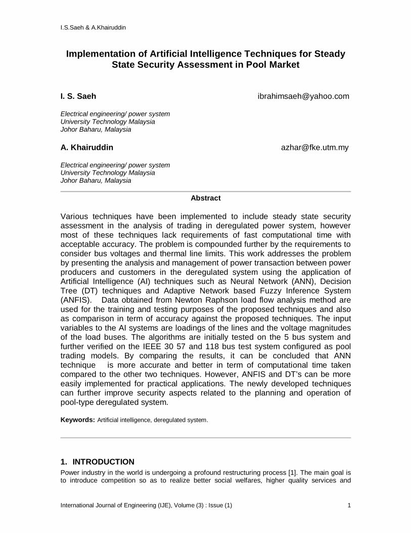
Implementation of Artificial Intelligence Techniques for Steady State Security Assessment in Pool Market
I. S. Saeh [email protected] Electrical engineering/ power system University Technology Malaysia Johor Baharu, Malaysia A. Khairuddin [email protected] Electrical engineering/ power system University Technology Malaysia Johor Baharu, Malaysia
Abstract
Various techniques have been implemented to include steady state security assessment in the analysis of trading in deregulated power system, however most of these techniques lack requirements of fast computational time with acceptable accuracy. The problem is compounded further by the requirements to consider bus voltages and thermal line limits. This work addresses the problem by presenting the analysis and management of power transaction between power producers and customers in the deregulated system using the application of Artificial Intelligence (AI) techniques such as Neural Network (ANN), Decision Tree (DT) techniques and Adaptive Network based Fuzzy Inference System (ANFIS). Data obtained from Newton Raphson load flow analysis method are used for the training and testing purposes of the proposed techniques and also as comparison in term of accuracy against the proposed techniques. The input variables to the AI systems are loadings of the lines and the voltage magnitudes of the load buses. The algorithms are initially tested on the 5 bus system and further verified on the IEEE 30 57 and 118 bus test system configured as pool trading models. By comparing the results, it can be concluded that ANN technique is more accurate and better in term of computational time taken compared to the other two techniques. However, ANFIS and DT’s can be more easily implemented for practical applications. The newly developed techniques can further improve security aspects related to the planning and operation of pool-type deregulated system. Keywords: Artificial intelligence, deregulated system.
1. INTRODUCTION Power industry in the world is undergoing a profound restructuring process [1]. The main goal is to introduce competition so as to realize better social welfares, higher quality services and

I.S.Saeh & A.Khairuddin
International Journal of Engineering (IJE), Volume (3) : Issue (1) 2
improved investment efficiency. Security is defined as the capability of guaranteeing the continuous operation of a power system under normal operation even following some significant perturbations [2]. The new environment raises questions concerning all sectors of electric power industry. Nevertheless, transmission system is the key point in market development of a deregulated market since it puts constraints to the market operation due to technical requirements. Especially, in systems having weak connections among areas, congestion problems arise due to line overloading or to voltage security requirements especially during summer [3]. The deregulation of the electric energy market has recently brought to a number of issues regarding the security of large electrical systems. The occurrence of contingencies may cause dramatic interruptions of the power supply and so considerable economic damages. Such difficulties motivate the research efforts that aim to identify whether a power system is insecure and to promptly intervene. In this paper, we shall focus on Artificial Intelligence for the purpose of steady state security assessment and rapid contingency evaluation [4]. For reliability analysis of fault-tolerant multistage interconnection networks an irregular augmented baseline network (IABN) is designed from regular augmented baseline network (ABN) [5]. In the past, the electric power industry around the world operated in a vertically integrated environment. The introduction of competition is expected to improve efficiency and operation of power systems. Security assessment, which is defined as the ability of the power system to withstand sudden disturbances such as electric short circuits or unanticipated loss of system load, is one of the important issues especially in the deregulated environment [6]. When a contingency causes the violation of operating limits, the system is unsafe. One of the conventional methods in security assessment is a deterministic criterion, which considers contingency cases, such as sudden removals of a power generator or the loss of a transmission line. Such an approach is time consuming for operating decisions due to a large number of contingency cases to be studied. Moreover, when a local phenomenon, such as voltage stability is considered for contingency analysis, computation burden is even further increased. This paper tries to address this situation by treating power system security assessment as a pattern classification problem. A survey of several power flow methods are available to compute line flows in a power system like Gauss Seidel iterative method, Newton-Raphson method, and fast decoupled power flow method and dc power flow method but these are either approximate or too slow for on-line implementation in [7,8].With the development of artificial intelligence based techniques such as artificial neural network, fuzzy logic etc. in recent years, there is growing trend in applying these approaches for the operation and control of power system [8,9]. Artificial neural network systems gained popularity over the conventional methods as they are efficient in discovering similarities among large bodies of data and synthesizing fault tolerant model for nonlinear, partly unknown and noisy/ corrupted system. Artificial neural network (ANN) methods when applied to Power Systems Security Assessment overcome these disadvantages of the conventional methods. ANN methods have the advantage that once the security functions have been designed by an off-line training procedure, they can be directly used for on-line security assessment of Power Systems. The computational effort for on-line security assessment using real-time systems data and for security function is very small. The previous work (10,11,12,13) have not addressed the issue of large number of possible contingencies in power system operation. Current work has developed static security assessment using ANN with minimum number of cases from the available large number of classified contingencies. The proposed methodology has led to reduction of computational time with acceptable accuracy for potential application in on line security
assessment. Most of the work in ANN has not concentrated on developing algorithms for ranking contingencies in terms of their impact on the network performance. Such an approach is described in Ref. [14], where DTs are coupled with ANNs. The leading idea is to preserve the advantages of both DTs and ANNs while evading their weaknesses [15].A review of existing methods and techniques are presented in [16]. A wide variety of ML techniques for solving timely problems in the areas of Generation, Transmission and Distribution of modern Electric Energy Systems have been proposed, Decision

I.S.Saeh & A.Khairuddin
International Journal of Engineering (IJE), Volume (3) : Issue (1) 3
Trees, Fuzzy Systems and Genetic Algorithms have been proposed or applied to security assessment[17] such as Online Dynamic Security Assessment Scheme[18]. 3 Existing Models of Deregulation The worldwide current developments towards deregulation of power sector can be broadly classified in following three types of models [19]. 3.1 Pool model In this model the entire electricity industry is separated into generation (gencos), transmission (transcos) and distribution (discos) companies. The independent system operator (ISO) and Power exchanger (PX) operates the electricity pool to perform price-based dispatch of power plants and provide a form for setting the system prices and handling electricity trades. In some cases transmission owners (TOs) are separated from the ISO to own and provide the transmission network. The England & Wales model is typical of this category. The deregulation model of Chile, Argentina and East Australia also fall in this category with some modifications. 3.2 Pool and bilateral trades model In this model participant may not only bid into the pool through power exchanger (PX), but also make bilateral contracts with others through scheduling coordinators (SCs). Therefore, this model provides more flexible options for transmission access. The California model is of this category. The Nordic model and the New Zeeland model almost fall into this category with some modifications. 3.3 Multilateral trades model This model envisages that multiple separate energy markets, dominated by multilateral and bilateral transactions, which coexist in the system and the concept of pool and PX disappear into this multi-market structure. Other models such as the New York Power Pool (NYPP) model fall somewhere in between these three models. 4 ARTIFICIAL INTELLIGENCE (AI) METHODS Artificial Neural Networks (ANNs), Decision Trees (DTs) and Adaptive Network based Fuzzy Inference System (ANFIS) belong to the Machine Learning (ML) or Artificial Intelligence (AI) methods. Together with the group of statistical pattern recognition, they form the general class of supervised learning systems. And while their models are quite different, their objective of classification and prediction remains the same; to reach this objective, learning systems examine sample solved cases and propose general decision rules to classify new ones; in other words, they use a general “pattern recognition” (PR) type of approach. For the Static Security Analysis the phenomenon is the secure or insecure state of the system characterized by violation of voltage and loading limits, and the driving variables, called attributes, are the control variables of the system. In the problem examined the objects are pre fault operating states or points (OPs) defined by the control variables of the System and are partitioned in two classes, i.e. SAFE or UNSAFE. AI's when used for static security assessment, operate in two modes: training and recall (test). In the training mode, the AI learns from data such as real measurements of off-line simulation. In the recall mode, the AI can provide an assessment of system security even when the operating conditions are not contained in the training data. 4.1 Artificial Neural Networks (ANNs)

I.S.Saeh & A.Khairuddin
International Journal of Engineering (IJE), Volume (3) : Issue (1) 4
ANN is an intelligent technique, which mimics the functioning of a human brain. It simulates human intuition in making decision and drawing conclusions even when presented with complex, noisy, irrelevant and partial information. ANN’s systems gained popularity over the conventional methods as they are efficient in discovering similarities among large bodies of data and synthesizing fault tolerant model for nonlinear, partly unknown and noisy/ corrupted system. An artificial neural network as defined by Hect-Nielsen [20] is a parallel, distributed information processing structure consisting of processing elements interconnected via unidirectional signal channels called connections or weights. There are different types of ANN where each type is suitable for a specific application. ANN techniques have been applied extensively in the domain of power system. Basically an ANN maps one function into another and they can be applied to perform pattern recognition, pattern matching, pattern classification, pattern completion, prediction, clustering or decision making. Back propagation (BP) training paradigm also successfully describe by [21]. The compromise for achieving on-line speed is the large amounts of processing required off-line [22]. ANN have shown great promise as means of predicting the security of large electric power systems [23].Several NN’s techniques have been proposed to assess static security like Kohonen self-organizing map (SOM) [24]. Artificial Neural Network Architecture is shown in figure 1.
Figure1 Artificial Neural Network Architecture 4.2 Adaptive Network Fuzzy Inference System Adaptive Network based Fuzzy Inference System (ANFIS) [25] represents a neural network approach to the design of fuzzy inference system. A fuzzy inference system employing fuzzy if-then rules can model the qualitative aspects of human knowledge and reasoning processes without employing precise quantitative analyses. This fuzzy modeling, first explored systematically by Takagi and Sugeno [26], has found numerous practical applications in control, prediction and inference. By employing the adaptive network as a common framework, other adaptive fuzzy models tailored for data classification is proposed [27]. We shall reconsider an ANFIS originally suggested by R. Jang that has two inputs, one output and its rule base contains two fuzzy if-then rules:
Rule 1: If x is 1A and y is 1B , then 1f = ,111 ryqxp (1)
Rule2: If x is 2A and y is 2B , then 2f = 2p + ,22 ryq (2) The five-layered structure of this ANFIS is depicted in Figure 2 and brief description of each layer function is discussed in [28].

I.S.Saeh & A.Khairuddin
International Journal of Engineering (IJE), Volume (3) : Issue (1) 5
Figure2 An Adaptive Network Architectures
4.3 Decision Tree’s Decision Tree is a method for approximating discrete-valued target functions, in which the learned function is presented by a decision tree. Learned trees can also be re-represented as sets of if-then roles to improve human readability. These learning methods are among the most popular of inductive inference algorithms. The DT is composed of nodes and arcs [29]. Each node refers to a set of objects, i.e. a collection of records corresponding to various OPs. The root node refers to the whole LS. The decision to expand a node n and the way to perform this expansion rely on the information contained in the corresponding subset En of the LS.Thus, a node might be a terminal (leaf) or a nonterminal node (split). If it is a non-terminal node, then it involves a test which partitions its set into two disjoint subsets. If the node is a terminal one, then it carries a class label, i.e. system in SAFE or UNSAFE operating state. Figure (2) illustrates the system status and view tree. The main advantage of the DTSA approach is that it will enable one to exploit easily the very fast growing of computing powers. While the manual approach is “bottle-necked” by the number. General DT’s methodology [30] and [31] .The procedure for building the Decision Tree is presented in [30]. The application of decision trees to on-line steady state security assessment of a power system has also been proposed by Hatziargyriou et al [32]. (Albuyeth et al.1982, Ejebe &Wellenberrg, 1979, etc)[33-34] respectively, these involve overloaded lines, or bus voltages that deviate from the normal operation limits. 5 RESULTS AND DISSCUSION For the purpose of illustrating the functionality and applicability of the proposed techniques, the methodology of each technique has been programmed and tested on several test systems such as 5, 30, 57 and 118 IEEE test system. The results obtained from all techniques are compared in order to determine the advantages of any technique compared to others in terms of accuracy against the benchmark technique and computational time taken, as well as to study the feasilibility to improve the techniques further. For the same data (train, test data) and the same system ANN, ANFIS and DT techniques are used to examine whether the power system is secured under steady-state operating conditions. The AI techniques gauge the bus voltages and the line flow conditions. For training, data obtained from Newton Raphson load flow analysis are used. The test has been performed on 5-IEEE bus system.
Figure 3 shows the topology of the system
The IEEE-5 bus is the test system which contains 2 generators, 5 buses and 7 lines. The topology of this system is shown in Figure 3.

I.S.Saeh & A.Khairuddin
International Journal of Engineering (IJE), Volume (3) : Issue (1) 6
Figure 3: The Topology of IEEE 5bus System
Figure 4: NR, ANN, ANFIS and DT performance comparison Using the same input data, comparing ANFIS , ANN and DT against NR results, it is observed that NN has got acceptable results (classification).In figure(4) we consider the result over 0.5 is in security region while pointes below it is in insecurity region, in this case, 0.5 is then as cut-off point for security level. NN results have got one misclassification, it was found in pattern 8. For ANFIS the misclassification was12, 15, 23, 24 and 25 5 neurons, while for DT results have got one misclassification, it was found in pattern 7,8,11,13,14,15,21,22,23and 24 ,and as result the ANN is better than ANFIS in term of static security assessment. Table 1 compares ANN, ANFIS and DT against the load flow results using Newton Raphson method for static security assessment classification in term of accuracy. It can be seen that ANN got better results in term of accuracy (96.29), and ANFIS was (81.48) while DT was (74.07).
Table1: LOAD FLOW, ANN, ANFIS, and DT COMPARISON
Table 2 shows the number of neurons in the training and the testing mode for each test system.
Table 2: Number of Neurons in the Train and the Test Mode
Methods Load Flow ANN ANFIS DT
Accuracy (100%) 100 96.29 81.48 74.07

I.S.Saeh & A.Khairuddin
International Journal of Engineering (IJE), Volume (3) : Issue (1) 7
5.1 Decision Tree’s Comparison The five types of decision trees are compared in term of accuracy, computational time and root mean square error (RMSE) and then we will use the better for the artificial intelligence techniques comparison. The following Tables 3-a and 3-b illustrate this comparison in the train and test mood.
Table 3-a: Training Decision Trees comparison
Table 3-b: Testing Decision Trees comparison
From these tables, it can be seen that in the training mode all types of DT technique achieve acceptable accuracy (100%) while in term of the computational time, the J48 type has the best result (0.001 sec.).In the testing mode, we can say that both J48 and Random Tree got better accuracy(95.66,96.55 %) respectively, while in the aspect of the computational time we found that Random Tree is better(0.001 sec.). As a result, we select Random Tree for the comparison of DT against ANN and ANFIS. 5.2 AI Techniques Comparison A comparison in term of accuracy between ANN, ANFIS and Random Tree for 5, 30, 57 and 118 IEEE bus test system is presented in next two tables. In table (4), the result shows that in the train mood Random Tree got better results 100%) and the overall results are acceptable.
Table4: Train AI comparison
In the table (5) we illustrate the comparison in the test mood for the 5, 30,57and 118 test system and it can be seen clearly that ANN got better accuracy in the all system used. And as result we recommend ANN. 5.3 ANN IMPLEMENTATION FOR THE DEREGULATED SYSTEM

I.S.Saeh & A.Khairuddin
International Journal of Engineering (IJE), Volume (3) : Issue (1) 8
In the current work, we attempt to implement static security assessment methodology for pool trading type of deregulated environment. The implementation is to be tested on several test systems, i.e. 5- bus.
AI BUS NO. ANN ANFIS RANDOM
TREE 5 95.65 91.30 95.55 30 97.77 90.44 94.44 57 96.87 85.79 92.56
118 98.88 80.45 92
Table5: Test AI comparison
It is to be noted here, that the trading in this paper is from the view of security so that the pricing is not taken into account. In the tables below A, B, C and D are generation companies (GenCo.) while A1, B1, C1and D1 are customers companies (DesCo.) which put their bids in the spot market with their amounts and prices.
Table6-a: GenCo. Names, Amounts and Prices
Table6-b: GenCo. Names, Amounts and Prices As to be mentioned later, we take only security in the account, the procedure in this type of trading is:
A1 ask from the market 15 MW, the lowest price in the generation companies which is here C can gives the 10 MW and test for the security.
A1 needs 5 MW, so B can give this amount because B is the lowest price after C and check for the security.
B1 ask for 10 MW, the rest of the amount of B can be given to B1, and check for the security also.
C1 ask for 25 MW it can be given as folow:5 MW from D and the rest from A Finally, D1 ask only 5 MW it will be given from the rest of the amount of D1, table (7)
shows all of these trading process.
I.S.Saeh & A.Khairuddin
International Journal of Engineering (IJE), Volume (3) : Issue (1) 9
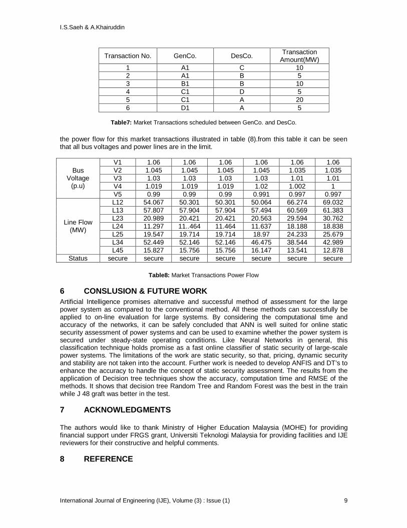
Transaction No. GenCo. DesCo. Transaction Amount(MW)
1 A1 C 10 2 A1 B 5 3 B1 B 10 4 C1 D 5 5 C1 A 20 6 D1 A 5
Table7: Market Transactions scheduled between GenCo. and DesCo.
the power flow for this market transactions illustrated in table (8).from this table it can be seen that all bus voltages and power lines are in the limit.
V1 1.06 1.06 1.06 1.06 1.06 1.06 V2 1.045 1.045 1.045 1.045 1.035 1.035 V3 1.03 1.03 1.03 1.03 1.01 1.01 V4 1.019 1.019 1.019 1.02 1.002 1
Bus Voltage
(p.u) V5 0.99 0.99 0.99 0.991 0.997 0.997 L12 54.067 50.301 50.301 50.064 66.274 69.032 L13 57.807 57.904 57.904 57.494 60.569 61.383 L23 20.989 20.421 20.421 20.563 29.594 30.762 L24 11.297 11..464 11.464 11.637 18.188 18.838 L25 19.547 19.714 19.714 18.97 24.233 25.679 L34 52.449 52.146 52.146 46.475 38.544 42.989
Line Flow (MW)
L45 15.827 15.756 15.756 16.147 13.541 12.878 Status secure secure secure secure secure secure secure
Table8: Market Transactions Power Flow
6 CONSLUSION & FUTURE WORK Artificial Intelligence promises alternative and successful method of assessment for the large power system as compared to the conventional method. All these methods can successfully be applied to on-line evaluation for large systems. By considering the computational time and accuracy of the networks, it can be safely concluded that ANN is well suited for online static security assessment of power systems and can be used to examine whether the power system is secured under steady-state operating conditions. Like Neural Networks in general, this classification technique holds promise as a fast online classifier of static security of large-scale power systems. The limitations of the work are static security, so that, pricing, dynamic security and stability are not taken into the account. Further work is needed to develop ANFIS and DT’s to enhance the accuracy to handle the concept of static security assessment. The results from the application of Decision tree techniques show the accuracy, computation time and RMSE of the methods. It shows that decision tree Random Tree and Random Forest was the best in the train while J 48 graft was better in the test. 7 ACKNOWLEDGMENTS The authors would like to thank Ministry of Higher Education Malaysia (MOHE) for providing financial support under FRGS grant, Universiti Teknologi Malaysia for providing facilities and IJE reviewers for their constructive and helpful comments.
8 REFERENCE

I.S.Saeh & A.Khairuddin
International Journal of Engineering (IJE), Volume (3) : Issue (1) 10
1. Lai Loi Lai, “Power System Restructuring and Deregulation”, John Wiley and Sons, Ltd., 2001.
2. Task Force 21 of Advisory Group 02 of Study Committee 38, ”Power System Security Assessment”, CIGRE Technical Brochure, Tech. Rep.,2004.
3. C. Vournas, V. Nikolaidis, and A. Tassoulis, “Experience from the Athens blackout of july 12, 2004,” IEEE Saint Petersburg Power Tech 27-30 June 2005.
4. H. Rudnick, R. Palma, J. E. Fernandez: “Marginal Pricing and Supplement Cost Allocation in Transmission Open Access”, IEEE Transactions on Power Systems, Vol. 10, No. 2, pp 1125-1132,1995.
5. Rinkle Aggarwal & Dr. Lakhwinder Kaur“On Reliability Analysis of Fault-tolerant Multistage Interconnection Networks” International Journal of Computer Science & Security, Volume (2): Issue (4), pp, 1-8, November, 2008.
6. Hiromitsu Kumamoto, Ernest J. Henley. Probabilistic Risk Assessment and Management for Engineers and Scientists (Second Edition). IEEE Press, 1996, USA.
7. N. Kumar, R. Wangneo, P.K. Kalra, S.C. Srivastava, Application of artificial neural network to load flow, in: Proceedings TENCON’91,IEE Region 10 International Conference on EC3-Energy, Computer, Communication and Control System, vol. 1, 1991, pp. 199–203.
8. S. Sharma, L. Srivastava, M. Pandit, S.N. Singh, Identification and determination of line overloading using artificial neural network, in: Proceedings of International Conference, PEITSICON-2005, Kolkata (India), January 28–29, (2005), pp. A13 A17.
9. V.S. Vankayala, N.D. Rao, Artificial neural network and their application to power system—a bibliographical survey, Electric Power System Research 28 (1993) 67–69.
10. R. Fischl, T. F. Halpin, A. Guvenis, "The application of decision theory to contingency selection," IEEE Trans. on CAS, vo.11, 29, pp.712-723, Nov. 1982.
11. M. E. Aggoune, L. E. Atlas, D. A. Cohn, M. A. El-Sharkawi and R J. Marks, "Artificial Neural Networks for Power System Static Security Assessment," IEEE International Symposium on Circuits and Systems, Portland, Oregon, May 9 -11, 1989, pp. 490-494.
12. Niebur D., Germond A. J. “Power System Static Security Assessment Using the Kohonen Neural Network Classifier”, IEEE Trans. on Power Systems, Vol. 7, NO. 2, pp. 270-277, 1992.
13. Craig A. Jensen, Mohamed A. El-Sharkawi, and Robert J. Marks,” Power System Security Assessment Using Neural Networks: Feature Selection Using Fisher Discrimination” IEEE Transactions on Power Systems, vol. 16, no. 4, November 2001, pp 757-763.
14. Wehenkel, I, and Akella, V.B.: ’A Hybrid Decision Tree - Neural Network Approach for Power System Dynamic Security Assessment’. ESAP’93, 4th Symp. on Expert Systems Application to Power Systems, pp. 285-291, 1993.
15. L. Wehenkel and M. Pavella, “Advances in Decision Trees Applied to Power System Security Assessment,” Proc. IEE Int’l Conf. Advances in Power System Control, Operation and Management, Inst. Electrical Engineers, Hong Kong, 1993, pp. 47–53.
16. K.S.Swarup, RupeshMastakar, K.V.Parasad”Decision Tree for steady state security assessment and evaluation of power system” Proceeding of IEEE, ICISIP-2005, PP211-216.
17. Louis Wehenkel”Machine-Learning Approaches to Power-System Security Assessment”IEEE Expert, pp, 60-72, 1997.
18. Kai Sunand Siddharth Likhate et al” An Online Dynamic Security Assessment Scheme Using Phasor Measurements and Decision Trees” IEEE Transactions On Power Systems, vol. 22, NO. 4, November 2007,pp,1935-1943.
19. Padhy, N.P.; Sood, Y.R.; ‘’Advancement in power system engineering education and research with power industry moving towards deregulation’’Power Engineering Society General Meeting, 2004. IEEE, 6-10 June 2004 Page(s):71 - 76 Vol.1.
20. Hect-Nielsen, R. 'Theory of the Backpropagation Neural Network.", Proceeding of the International Joint Confernce on Neural Network June 1989, NewYork: IEEE Press, vol.I, 593 611.
21. R C Bansal“Overview and Literature Survey of Artificial Neural Networks Applications to Power Systems (1992-2004)” IE (I) Journal, pp282-296, 2006.

I.S.Saeh & A.Khairuddin
International Journal of Engineering (IJE), Volume (3) : Issue (1) 11
22. Sidhu, T.S., Lan Cui. “Contingency Screening for Steady-State Security Analysis by Using Fft and Artificial Neural Networks.” IEEE Transactions on Power Systems, Vol. 15, pp: 421 – 426, 2000.
23. D.J. Sobajic & Y.H. Pao, Artificial neural-net based dynamic security assessment, IEEE Transactions on Power Systems, vo.4,no.1, m1989, 220–228.
24. D. Niebur & A.J. Germond, Power system static security assessment using the Kohonen neural network classifier, IEEE Transactions Power Systems, vo7,no.2, 1992, 865–872.
25. J.S.R.Jang, "Anfis: Adaptive-network-based fuzzy inference systems",IEEE Transactions on Systems, Man and Cybernetics, vol.23, no.3, pp.665-685, 1993.
26. T. Takagi and M. Sugeno, “Fuzzy identification of systems and its applications to’ modeling and control,” IEEE Trans. Syst., Man, Cybern. vol. 15, pp. 116,132, 1985.
27. C.-T Sun and J.-S. Roger Jang, “Adaptive network based fuzzy classification,”in Proc.Japan-USA. Symp. Flexible Automat, July 1992.
28. J-S.R.Jang, C.-T.Sun.E.Mizutani, Neuro-Fuzzy and Soft Computing, Prentice Hall, Upper Saddle River, NJ, 1997.
29. Hatziqyriou, N.D., Contaxis, G.C. and Sideris, N.C. ’A decision tree method for on-line steady state security assessment’, IEEE PES Summer Meeting. paper No. 93SM527-2,1993.
30. K.S.Swarup, RupeshMastakar, K.V.Parasad”Decision Tree for steady state security assessment and evaluation of power system” Proceeding of IEEE, ICISIP-2005, PP211-216.
31. S. Papathanassiou N. Hatziargyriou and M. Papadopoulos. "Decision trees for fast security assessment of autonomous power systems with large penetration from renewables". IEEE Trans. Energy Conv., vol. 10, no. 2, pp.315-325, June 1995.
32. Hatziargyriou N.D., Contaxis G.C., Sideris N.C., “A decision tree method for on-line steady state security assessment”, IEEE Transactions on Power Systems, Vol. 9, No 2, p. 1052-1061, May 1994.
33. Albuyeh F., Bose A. and Heath B., “Reactive power considerations in automatic contingency selection”, IEEE Transactions on Power Apparatus and Systems, Vol. PAS-101, No. 1January 1982, p. 107.
34. Ejebe G.C., Wollenberg B.F., “Automatic Contingency Selection”, IEEE Trans. on Power Apparatus and Systems, Vol.PAS-98, No.1 Jan/Feb 1979 p.97.

Azadeh Khalatbari & Kouroush Jenab
International Journal of Engineering, Volume (3) : Issue (1) 12
Anesthesiology Risk Analysis Model
Azadeh Khalatbari [email protected] Department of Medicine University of Ottawa Ottawa, Ontario, Canada M5B 2K3
Kouroush Jenab [email protected] Department of Mechanical and Industrial Engineering Ryerson University Toronto, Ontario, Canada M5B 2K3
ABSTRACT
This paper focuses on the human error identified as an important risk factor in the occurrence of the anesthesia-related deaths. Performing clinical root cause analysis, the common anesthesia errors and their causes classified into four major problems (i.e., breathing, drug, technical, and procedural problems) are investigated. Accordingly, a qualitative model is proposed that analyzes the influence of the potential causes of the human errors in these problems, which can lead to anesthetic deaths. Using risk measures, this model isolates these human errors, which are critical to anesthesiology for preventive and corrective actions. Also, a Markovian model is developed to quantitatively assess the influence of the human errors in the major problems and subsequently in anesthetic deaths based on 453 reports over nine month. Keywords: Anesthesia, Medical Systems, Human Errors, Markov Model.
1. INTRODUCTION
Anesthesiology concerns with the process of turning a patient into insensitive to the pain, which results from chronic disease or during surgery. A variety of drugs and techniques can be used to maintain anesthesia. When anesthesia is induced, the patient needs respiratory support to keep the airway open, which requires special tools and techniques. For example, it is advantageous to provide a direct route of gases into the lungs, so an endotracheal tube is placed through the mouth into the wind pipe and connected to the anesthesia system. A cuff on the tube provides an airtight seal. To place the tube, the patient’s muscles must be paralyzed with a drug such as Curare. The drugs usually have some effects on the cardiovascular system. Therefore, anesthetist must monitor these effects (i.e., blood pressure, heart rate, etc). Unfortunately, there is not a fixed dose of most drugs used in anesthesia; rather, they are subjectively used by their effects on the patient. Generally, the anesthetist is engaged in a number of activities during the operation as follows: monitoring the patient and the life support, recoding the vital sings at least every 5 minutes, evaluating blood loss and urine output, adjusting the anesthetic level and administrating the medications, IV fluids, and blood, and adjusting the position of the operation room table. During this processes, there are some factors that cause complication or anesthetic death. In 1954, Beecher and Todd investigation on the deaths resulted from anesthesia and surgery showed that the ratio

Azadeh Khalatbari & Kouroush Jenab
International Journal of Engineering, Volume (3) : Issue (1) 13
of anesthesia-related death was 1 in 2680 [1]. In 1984, Davis and Strunin investigated the root causes of anesthetic-related death over 277 cases that depicted faulty procedure, coexistent disease, the failure of postoperative care, and drug overdose were major reasons of the deaths [2]. They showed the anesthetic-related death ratio was decreased from 1 in 2680 to 1 in 10000 because of taking pre-caution and post-caution measures. Even though human error was reported as a cause of anesthetic-related death for the first time in 1848, it took a long time to take the attention of the researchers toward such factor [3,4]. Cooper (1984) and Gaba (1989) studied human error in anesthetic mishaps in the United States that showed every year 2000 to 10000 patients die from anesthesia attributed reasons [5,6]. Reviewing the critical incidents in a teaching hospital, Short et al. (1992) concluded that human error was a major factor in 80% of the cases [7]. There exist some researches witnessed human error is a major factor in anesthesia-related deaths [8, 9, 10, 11]. In 2000, the role of fatigue in the medical incident was studied by reviewing 5600 reports in Australian incident monitoring database for the period of April 1987 to October 1997. In 2003, an anesthetic mortality survey conducted in the US that depicted the most common causes of perioperative cardiac arrest were medication events (40%), complications associated with central venous access (20%), and problems in airways management (20%). Also, the risk of death related to anesthesia-attributed perioperative cardiac arrest was 0.55 per 10,000 anesthetics [13]. In 2006, among the 4,200 death certificates analyzed in France, 256 led to a detailed evaluation, which depicted the death rates totally or partially related to anesthesia for 1999 were 0.69 in 100,000 and 4.7 in 100,000 respectively [14, 15]. In Anesthesiology, human error is defined either as an anesthesiologist’s decision, which leads to an adverse outcome or an anesthesiologist’s action, which is not in accordance with the anesthesiology protocol. In this paper, we study the frequent anesthesia errors, their causes, and modes of human error in anesthesia in order to develop qualitative and quantitative models for assessing the influence of the human errors in anesthetic deaths. Subsequently, a rule of thumb is proposed to reduce the influence on human errors in anesthetic deaths.
2. COMMON HUMAN ERRORS AND THEIR CAUSES IN ANESTHESIOLOGY
Figure 1 shows four types of anesthetic problems that can cause complication or death. The cause and effect diagram presents breathing, drug, procedural and technical problems, which can be triggered by common anesthesia errors.
Human error no.: 2,3,4,5,6,8,10,11,12,13,14,16
2- Syringe swap -------------->
10- Unintentional extubation ->
11- Misplaced tracheal tube ---> Human error no.: 1,2,3,6,11,12,17
12- Breathing circuit misconnection ---->
13- Inadequate fluid replacement -----> 1-
14- Premature extubation ----------------------> -->
16- Improper use of blood pressure monitor 5- Disconnection of intravenous line --->
18- 6- Vaporizer off unintentionally ---->
----------> 9- Breathing circuit leakage ------->
20- Incorrect IV line used --------------------------> 21- Hypoventilation ----------------------->
19- Laryngoscope failure -----------------------> 22- Incorrect drug selection ------>
17- Breathing circuit control technical error 8- Drug Overdose (Syringe, Vaporizer)
15- Ventilator failure -------------------> 7- Drug ampoule swap ---------------->
4- Loss of gas supply ----------------->
3- Gas flow control --------------->
Human error no.: 4,5,8,10,11,12,13,14,15,16,18,19
Human error no.: 1,7,9,17,19
Breathing circuit disconnection
during mechanical ventilation
Incorrect selection of airway
management method
Anesthestic-Related
Deaths
Breathing Error
Drug Error
Technical Error
Procedural Error
FIGURE 1: Cause and effect diagram for anesthesia-related deaths

Azadeh Khalatbari & Kouroush Jenab
International Journal of Engineering, Volume (3) : Issue (1) 14
Using root cause analysis, Table 1 presents the common anesthesia errors and their risk priority number (RPN). The RPN value for each potential error can be used to compare the errors identified within the analysis in order to make the corresponding improvement scheme. Using Tables 2 and 3, the RPN is multiplication of the rank of occurrence frequency and of the rank of severity. These common errors can result from human errors, which are believed to be responsible for 87% of the cases, presented in Table 4. The human errors contributing in the anesthetic error are indicated in the cause and effect diagram in Figure 2. This qualitative diagram along with RPN points out the required modifications to reduce the ratio of anesthesia-related deaths.
Code Error No. Description R.P.N
C01 1- Breathing circuit disconnection during mechanical ventilation 90
C02 2- Syringe swap 90
C03 3- Gas flow control 81
C04 4- Loss of gas supply 72
C05 5- Disconnection of intravenous line 72
C06 6- Vaporizer off unintentionally 64
C07 7- Drug ampoule swap 56
C08 8- Drug Overdose (Syringe, Vaporizer) 56
C09 9- Breathing circuit leakage 56
C10 10- Unintentional extubation 49
C11 11- Misplaced tracheal tube 42
C12 12- Breathing circuit misconnection 42
C13 13- Inadequate fluid replacement 42
C14 14- Premature extubation 36
C15 15- Ventilator failure 30
C16 16- Improper use of blood pressure monitor 25
C17 17- Breathing circuit control technical error 20
C18 18- Incorrect selection of airway management method 16
C19 19- Laryngoscope failure 12
C20 20- Incorrect IV line used 8
C21 21- Hypoventilation 4
C22 22- Incorrect drug selection 2
Table 1: Common anesthesia errors
Azadeh Khalatbari & Kouroush Jenab
International Journal of Engineering, Volume (3) : Issue (1) 15
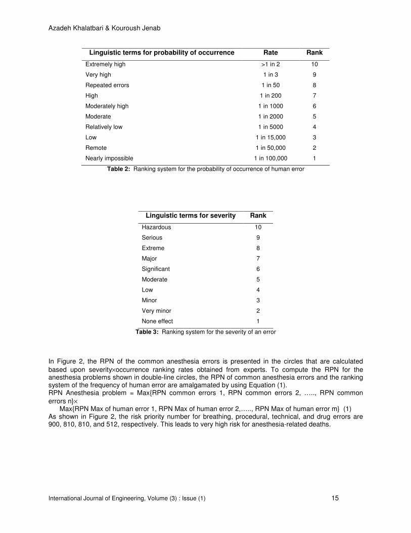
Linguistic terms for probability of occurrence Rate Rank
Extremely high >1 in 2 10
Very high 1 in 3 9
Repeated errors 1 in 50 8
High 1 in 200 7
Moderately high 1 in 1000 6
Moderate 1 in 2000 5
Relatively low 1 in 5000 4
Low 1 in 15,000 3
Remote 1 in 50,000 2
Nearly impossible 1 in 100,000 1
Table 2: Ranking system for the probability of occurrence of human error
Linguistic terms for severity Rank
Hazardous 10
Serious 9
Extreme 8
Major 7
Significant 6
Moderate 5
Low 4
Minor 3
Very minor 2
None effect 1
Table 3: Ranking system for the severity of an error
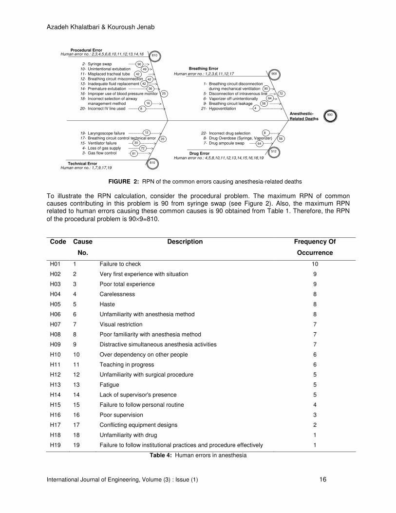
In Figure 2, the RPN of the common anesthesia errors is presented in the circles that are calculated
based upon severity×occurrence ranking rates obtained from experts. To compute the RPN for the anesthesia problems shown in double-line circles, the RPN of common anesthesia errors and the ranking system of the frequency of human error are amalgamated by using Equation (1). RPN Anesthesia problem = Max{RPN common errors 1, RPN common errors 2, ….., RPN common
errors n}× Max{RPN Max of human error 1, RPN Max of human error 2,….., RPN Max of human error m} (1) As shown in Figure 2, the risk priority number for breathing, procedural, technical, and drug errors are 900, 810, 810, and 512, respectively. This leads to very high risk for anesthesia-related deaths.
Azadeh Khalatbari & Kouroush Jenab
International Journal of Engineering, Volume (3) : Issue (1) 16
Human error no.: 2,3,4,5,6,8,10,11,12,13,14,16
2- Syringe swap -------------->
10- Unintentional extubation ->
11- Misplaced tracheal tube ---> Human error no.: 1,2,3,6,11,12,17
12- Breathing circuit misconnection ---->
13- Inadequate fluid replacement -----> 1-
14- Premature extubation ----------------------> -->
16- Improper use of blood pressure monitor 5- Disconnection of intravenous line --->
18- 6- Vaporizer off unintentionally ---->
--------> 9- Breathing circuit leakage ------->
20- Incorrect IV line used --------------------------> 21- Hypoventilation ----------------------->
19- Laryngoscope failure -----------------------> 22- Incorrect drug selection ------>
17- Breathing circuit control technical error 8- Drug Overdose (Syringe, Vaporizer)
15- Ventilator failure -------------------> 7- Drug ampoule swap ---------------->
4- Loss of gas supply ----------------->
3- Gas flow control --------------->
Human error no.: 4,5,8,10,11,12,13,14,15,16,18,19
Human error no.: 1,7,9,17,19
Breathing circuit disconnection
during mechanical ventilation
Incorrect selection of airway
management method
Anesthestic-
Related Deaths
Breathing Error
Drug Error
Technical Error
Procedural Error
90
49
42
42
42
36
25
16
8
810
12
900
810
512
2030
72
81
90
72
56
4
64
8
56
64
900
FIGURE 2: RPN of the common errors causing anesthesia-related deaths
To illustrate the RPN calculation, consider the procedural problem. The maximum RPN of common causes contributing in this problem is 90 from syringe swap (see Figure 2). Also, the maximum RPN related to human errors causing these common causes is 90 obtained from Table 1. Therefore, the RPN
of the procedural problem is 90×9=810.
Code Cause
No.
Description Frequency Of
Occurrence
H01 1 Failure to check 10
H02 2 Very first experience with situation 9
H03 3 Poor total experience 9
H04 4 Carelessness 8
H05 5 Haste 8
H06 6 Unfamiliarity with anesthesia method 8
H07 7 Visual restriction 7
H08 8 Poor familiarity with anesthesia method 7
H09 9 Distractive simultaneous anesthesia activities 7
H10 10 Over dependency on other people 6
H11 11 Teaching in progress 6
H12 12 Unfamiliarity with surgical procedure 5
H13 13 Fatigue 5
H14 14 Lack of supervisor's presence 5
H15 15 Failure to follow personal routine 4
H16 16 Poor supervision 3
H17 17 Conflicting equipment designs 2
H18 18 Unfamiliarity with drug 1
H19 19 Failure to follow institutional practices and procedure effectively 1
Table 4: Human errors in anesthesia
Azadeh Khalatbari & Kouroush Jenab
International Journal of Engineering, Volume (3) : Issue (1) 17
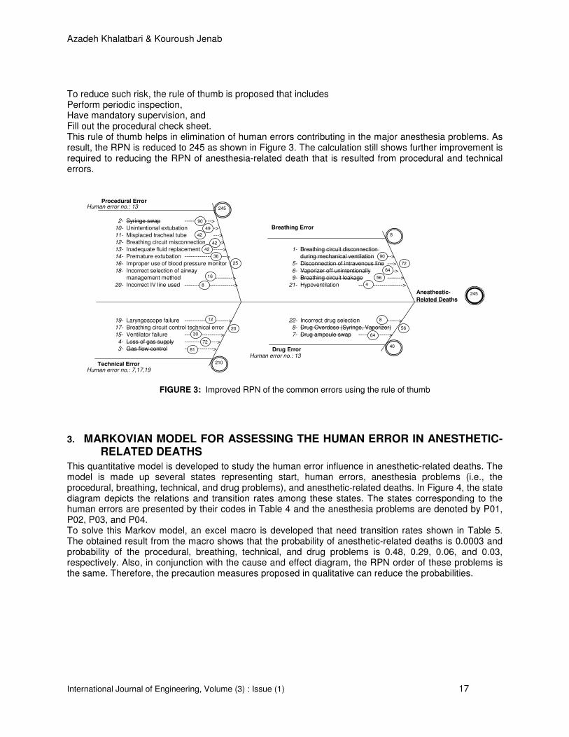
To reduce such risk, the rule of thumb is proposed that includes Perform periodic inspection, Have mandatory supervision, and Fill out the procedural check sheet. This rule of thumb helps in elimination of human errors contributing in the major anesthesia problems. As result, the RPN is reduced to 245 as shown in Figure 3. The calculation still shows further improvement is required to reducing the RPN of anesthesia-related death that is resulted from procedural and technical errors.
Human error no.: 13
2- Syringe swap -------------->
10- Unintentional extubation ->
11- Misplaced tracheal tube --->
12- Breathing circuit misconnection ---->
13- Inadequate fluid replacement -----> 1-
14- Premature extubation ----------------------> -->
16- Improper use of blood pressure monitor 5- Disconnection of intravenous line --->
18- 6- Vaporizer off unintentionally ---->
----------> 9- Breathing circuit leakage ------->
20- Incorrect IV line used --------------------------> 21- Hypoventilation ----------------------->
19- Laryngoscope failure -----------------------> 22- Incorrect drug selection ------>
17- Breathing circuit control technical error 8- Drug Overdose (Syringe, Vaporizer)
15- Ventilator failure -------------------> 7- Drug ampoule swap ---------------->
4- Loss of gas supply ----------------->
3- Gas flow control --------------->
Human error no.: 13
Human error no.: 7,17,19
Breathing circuit disconnection
during mechanical ventilation
Incorrect selection of airway
management method
Anesthestic-
Related Deaths
Breathing Error
Drug Error
Technical Error
Procedural Error
90
49
42
42
42
36
25
16
8
245
12
8
210
40
2030
72
81
90
72
56
4
64
8
56
64
245
FIGURE 3: Improved RPN of the common errors using the rule of thumb
3. MARKOVIAN MODEL FOR ASSESSING THE HUMAN ERROR IN ANESTHETIC-RELATED DEATHS
This quantitative model is developed to study the human error influence in anesthetic-related deaths. The model is made up several states representing start, human errors, anesthesia problems (i.e., the procedural, breathing, technical, and drug problems), and anesthetic-related deaths. In Figure 4, the state diagram depicts the relations and transition rates among these states. The states corresponding to the human errors are presented by their codes in Table 4 and the anesthesia problems are denoted by P01, P02, P03, and P04. To solve this Markov model, an excel macro is developed that need transition rates shown in Table 5. The obtained result from the macro shows that the probability of anesthetic-related deaths is 0.0003 and probability of the procedural, breathing, technical, and drug problems is 0.48, 0.29, 0.06, and 0.03, respectively. Also, in conjunction with the cause and effect diagram, the RPN order of these problems is the same. Therefore, the precaution measures proposed in qualitative can reduce the probabilities.

Azadeh Khalatbari & Kouroush Jenab
International Journal of Engineering, Volume (3) : Issue (1) 18
FIGURE 4: Anesthetic-related death state diagram
From To Rate (FITs) From To Rate (FITs)
H1 → H2 2002.5 H6 → P1 140.25
H1 → H3 1802.25 H6 → P2 140.25
H1 → H4 1802.25 H7 → P3 201.5
H1 → H5 1602 H8 → P1 152.25
H1 → H6 1602 H8 → P4 152.25
H1 → H7 1602 H9 → P3 329.75
H1 → H8 1401.75 H10 → P1 75
H1 → H9 934.5 H10 → P4 75
H1 → H10 934.5 H11 → P1 112.75
H1 → H11 801 H11 → P4 112.75
H1 → H12 801 H12 → P2 150
H1 → H13 667.5 H12 → P4 150
H1 → H14 333.75 H13 → P1 350
H1 → H15 333.75 H13 → P4 350
H1 → H16 267 H14 → P1 225
H1 → H17 80.1 H14 → P4 225
H1 → H18 53.4 H15 → P4 75
H1 → H19 13.35 H16 → P1 50
H2 → P1 306.5 H16 → P4 50
H2 → P2 306.5 H17 → P3 100
H3 → P1 256 H18 → P4 75
H3 → P2 256 H19 → P4 112.5
H4 → P1 505.25 P01 → END 28
Start
H09
H01
H17
H02
H12
H19 H18 H15 H07 H12
H05 H03 H06
H14
H13
H11
H04
H8
H10
H16
P04 P03
P02 P01
End-Anesthetic-
related Deaths

Azadeh Khalatbari & Kouroush Jenab
International Journal of Engineering, Volume (3) : Issue (1) 19
H4 → P4 505.25 P02 → END 22
H5 → P1 407 P03 → END 160
H5 → P4 407 P04 → END 150
Table 5: Transition rates of the anesthetic-related death Markov model
4. CONCLUSIONS
This paper studies the human errors in anesthesiology and measures the risk associated with these errors. The cause and effect diagram is used to identify the potential major problems in anesthesiology and their relationship with human errors, which may lead to death. The results depict the risk of anesthetic related death is very high and it can be reduced by applying simple rules that mitigate human errors. Also, Markovian model is used to compute the probabilities of occurrence of each major procedural, breathing, technical, and drug problems. In conjunction with the cause and effect results, this analysis confirms the procedural and breathing are utmost reported problems.
5. REFERENCES
HK. Beecher, DP. Todd. “A Study of the Deaths Associated with Anesthesia and Surgery Based on a Study of 599548 Anesthesia in ten Institutions 1948-1952”. Inclusive. Annals of Surgery, 140:2-35, 1954.
JM. Davies, L. Strunin. “Anethesia in 1984: How Safe Is It?”. Canadian Medical Association Journal, 131:437-441, 1984.
1. HK. Beecher. “The First Anesthesia Death with Some Remarks Suggested by it on the Fields of the Laboratory and the Clinic in the Appraisal of New Anesthetic Agents”. Anesthesiology, 2:443-449, 1941.
2. JB. Cooper, RS. Newbower, RJ. Kitz. “An Analysis of Major Errors and Equipment Failures in Anesthesia Management: Considerations for Prevention and Detection”. Anesthesiology, 60:34-42, 1984.
3. JB. Cooper, .Toward Prevention of Anesthetic Mishaps. International Anesthesiology Clinics, 22:167-183, 1984.
4. Gaba DM .Human Error in Anesthetic Mishaps. International Anesthesiology Clinics, 27(3):137-147, 1989.
5. Short TG, O’Regan A, Lew J, Oh TE .Critical Incident Reporting in an Anesthetic Department Quality Assurance Program. Anesthesia, 47:3-7., 1992.
6. Cooper JB, RS. Newbower, CD. Long. “Preventable Anesthesia Mishaps”. Anesthesiology, 49:399-406, 1978.
7. RD. Dripps, A. Lamont, JE. Eckenhoff. “The Role of Anesthesia in Surgical Mortality”. JAMA, 178:261-266, 1961.
8. C. Edwards, HJV. Morton, EA. Pask. “Deaths Associated with Anesthesia: Report on 1000 Cases”. Anesthesia, 11:194-220, 1956.

Azadeh Khalatbari & Kouroush Jenab
International Journal of Engineering, Volume (3) : Issue (1) 20
9. BS. Clifton, WIT Hotten. “Deaths Associated with Anesthesia”. British Journal of Anesthesia, 35:250-259, 1963.
10. GP. Morris, RW. Morris. “Anesthesia and Fatigue: An Analysis of the First 10 years of the Australian Incident Monitoring Study 1987-1997”. Anesthesia and Intensive Care, 28(3):300-303, 2000.
11. MC. Newland, SJ. Ellis, CA. Lydiatt, KR. Peters, JH. Tinker, DJ. Romberger, FA. Ullrich, and JR. Anderson. “Anesthetic-related cardiac arrest and its mortality: A report covering 72,959 anesthetics over 10 years from a U.S. teaching hospital”. Anesthesiology, 97:108-115, 2003.
12. A. Lienhart, Y. Auroy, F. Pequignot, D. Benhamou, J. Warszawski, M. Bovet, E. Jougla. “Survey of anesthesia-related mortality in France”. Anesthesiology, 105(6):1087-1097, 2006.
13. A. Wantanabe. “Human error and clinical engineering human error and human engineering”. 10(2):113-117, 1999.

Barbara Laskarzewska & Mehrab Mehrvar
International Journal of Engineering (IJE), Volume (3) : Issue (1) 21
Atmospheric Chemistry in Existing Air Atmospheric Dispersion Models and Their Applications: Trends, Advances and Future in Urban Areas in Ontario, Canada and in Other Areas of the World
Barbara Laskarzewska [email protected] Environmental Applied Science and Management Ryerson University 350 Victoria Street, Toronto Ontario, Canada, M5B 2K3
Mehrab Mehrvar [email protected] Department of Chemical Engineering Ryerson University 350 Victoria Street, Toronto Ontario, Canada, M5B 2K3
ABSTRACT
Air quality is a major concern for the public. Therefore, the reliability in modeling
and predicting the air quality accurately is of a major interest. This study reviews
existing atmospheric dispersion models, specifically, the Gaussian Plume models
and their capabilities to handle the atmospheric chemistry of nitrogen oxides
(NOx) and sulfur dioxides (SO2). It also includes a review of wet deposition in
the form of in-cloud, below cloud, and snow scavenging. Existing dispersion
models are investigated to assess their capability of handling atmospheric
chemistry, specifically in the context of NOx and SO2 substances and their
applications to urban areas. A number of previous studies have been conducted
where Gaussian dispersion model was applied to major cities around the world
such as London, Helsinki, Kanto, and Prague, to predict ground level
concentrations of NOx and SO2. These studies demonstrated a good agreement
between the modeled and observed ground level concentrations of NOx and SO2.
Toronto, Ontario, Canada is also a heavily populated urban area where a
dispersion model could be applied to evaluate ground level concentrations of
various contaminants to better understand the air quality. This paper also
includes a preliminary study of road emissions for a segment of the city of
Toronto and its busy streets during morning and afternoon rush hours. The
results of the modeling are compared to the observed data. The small scale
test of dispersion of NO2 in the city of Toronto was utilized for the local hourly

Barbara Laskarzewska & Mehrab Mehrvar
International Journal of Engineering (IJE), Volume (3) : Issue (1) 22
meteorological data and traffic emissions. The predicted ground level
concentrations were compared to Air Quality Index (AQI) data and showed a
good agreement. Another improvement addressed here is a discussion on
various wet deposition such as in cloud, below cloud, and snow.
Keywords: Air quality data, Air dispersion modeling, Gaussian dispersion model, Dry deposition, Wet
deposition (in-cloud, below cloud, snow), Urban emissions
1. INTRODUCTION
Over the past few years, the smog days in Ontario, Canada have been steadily increasing. Overall, longer smog episodes are observed with occurrences outside of the regular smog season. Air pollution limits the enjoyment of the outdoors and increases the cost of the health care [1] and [2]. To combat this problem, the Ontario Ministry of Environment (MOE) introduced new tools to reduce emissions as well as improved communication with the public on the state of the air quality. The communication policy has been implemented by the introduction of an Air Quality Index (AQI) based on actual pollutant concentrations reported by various monitoring stations across Ontario. One major concern is the spatial distribution of pollutants not captured by monitoring stations. To further enhance the understanding of pollution in an urban area, studies involving computational fluid dynamics (CFD) for street canyons, the land use regression (LUR), and the use of dispersion models have been conducted [3]. For a number of cities across the world dispersion models were applied to urban areas to understand pollution in a given city [4], [5], [6], [7] and [8]. The objective of these studies was to develop new air quality standards. These studies compared modeled ground level concentrations of NOx, SO2, and CO to the monitored data and showed a good agreement between observed and predicted data. Therefore, the main objectives of this study are to review the developments of Gaussian dispersion model, to review the dispersion modeling applied to urban areas, and to conduct a small scale test for the city of Toronto, Ontario, Canada. Over the years, the dispersion models have been used by the policy makers to develop air quality standards, an approach applicable to the city of Toronto, Ontario, Canada [10] and [11]. In 2005, fifteen smog advisories, a record number covering 53 days, were issued during smog season [12] in Toronto, Ontario, Canada. This is also a record number of days covering smog since the start of the Smog Alert Program in Ontario in 2002. Even more prominent was an episode that lasted 5 days in February 2005 and occurred outside smog season due to elevated levels of particulate matter with diameter less than 2.5 micrometers (PM2.5) followed by the earliest smog advisory ever issued during the normal smog season in April, 2005. As shown in Table 1, there has been an increase in smog advisories since 2002 [12], [13], [14] and [15].
TABLE 1: Summary of smog advisories issued from 2002 to 2005 in Ontario, Canada [12-15]

Barbara Laskarzewska & Mehrab Mehrvar
International Journal of Engineering (IJE), Volume (3) : Issue (1) 23
Year Number of Advisories Number of Days
2002 10 27 2003 7 19 2004 8 20 2005 15 53
Since 1999, each air quality study completed states that the air quality in Ontario is improving [12-18]. In 2005, the Ontario Medical Association (OMA) announced air pollution costs were estimated to be $507,000,000 in direct health care costs [1]. The OMA deems the cost to be an underestimate and a better understanding of air pollution and its effect on human health is required. In the past few years, a number of air initiatives have been established by the Ontario Ministry of the Environment (MOE). The initiatives include recently improved means of how the state of air quality is reported to the general public, the implementation of new regulations and mandates to reduce industrial emissions, and the review of the air quality standards for the province. For many that live in and around the Great Toronto Area (GTA), checking the AQI became a daily routine [19]. In recent years, AQI was reported to public using a new scale with a range of 1 to 100, good to very poor, respectively. Along with the quantitative scale, AQI lists the primary contaminant of greatest impact on human health which results in a poor air quality. Furthermore, the public is provided with a brief summary warning of how the pollutants affect vulnerable population so that necessary precautions may be undertaken. At the present time, the Ministry of the Environment utilizes data from Environment Canada’s Canadian Regional and Hemispheric Ozone and NOx System (CHRONOS), NOAA’s WRF/CHEM and NOAA-EPA NCEP/AQFS models to forecast air quality for the City of Toronto [20]. The primary objective is to forecast smog episodes. The AQI information is obtained via a network of 44 ambient air monitoring stations and 444 municipalities across Ontario [12] and [21]. In addition to improving public communication on the status of the air quality, the MOE established a set of new regulations targeting industries with the direct objectives to reduce emissions. Since the early 70’s, the MOE established a permitting system that set ground level limits. All industrial emitters were required by law, Section 9 of Canadian Environmental Protection Act (CEPA), to utilize an air dispersion model (Appendix A: Ontario Regulation 346 (O.Reg. 346)) and site specific emissions to demonstrate compliance against set ground level concentrations for the contaminants of interest. With time, the tools used to demonstrate compliance were clearly becoming out of date [22]. As the regulation aged, limitations began to slow the approval process and prevent certain applicants from obtaining permission to conduct work. It became apparent that in order to address the public concern, i.e., poor air quality, and pressure from industry, the MOE began to look into alternative solutions. In the 90’s, the MOE introduced a number of alternative permits and an Environmental Leaders program. The new permits (i.e. streamline review, the use of conditions in permits, and the comprehensive permits) were becoming ineffective as shown by the internal review of MOE’s work. Specifically, work was conducted by Standards Compliance Branch (SCB), former Environmental SWAT Team, and Selected Targets Air Compliance (STAC) department. The SCB’s work on regular basis demonstrated that approximately 60% of an industrial sector was found to be in non-compliance with provincial regulations [23]. The Environmental Leaders program is a program where companies are invited to sign up and are included under following conditions [24]:
a) commitment to voluntary reduction of emissions; and b) making production and emission data available to the public.
In exchange, Environmental Leaders program members are promised:
a) the public acknowledgement in MOE’s publications; and b) the recognition on the Ministry’s web site.

Barbara Laskarzewska & Mehrab Mehrvar
International Journal of Engineering (IJE), Volume (3) : Issue (1) 24
Currently, there are nine members listed on the MOE’s website [24]. As stated by the Industrial Pollution Team, the program was not effective in Ontario [24]. The report prepared by the Industrial Pollution Team specifically addresses the need to update tools (i.e. air dispersion models) utilized in the permitting process. Poor air quality, aging permitting system, and industries not committing to reduce emissions resulted in an overhaul of the system by implementation of the following new regulations:
1. Ontario Regulation 419/05, entitled “Air Pollution – Local Air Quality”, (O.Reg. 419/05) replaced O.Reg. 346 allowing companies to utilize new dispersion models: Industrial Source Complex – Short Term Model [Version 3]-Plume Rise Model Enhancements (ISC-PRIME), the American Meteorological Society/Environmental Protection Agency Regulatory Model Improvement Committee’s Dispersion Model (AERMOD) along with the establishment of new air standards [25];
2. Ontario Regulation 127/01, entitled “Airborne Contaminant Discharge Monitoring and Reporting”, (O.Reg. 127/01) which is an annual emissions reporting program due by June 1st each year [26];
3. Data from annual reporting programs was utilized to implement Ontario Regulation 194/05, entitled “Industrial Emissions – Nitrogen Oxides and Sulphur Dioxide”, (O.Reg. 194) which caps NOx and SOx emissions of very specific industries with set reduction targets [27]. The targets are intensity based. For industries that do not meet their targets, options of trading or paying for the emissions exist;
4. On the federal level, a National Pollutant Release Inventory (NPRI), a program similar to O.Reg. 127/01 which requires industries to submit an annual emissions report by June 1st each year [28];
5. On the federal level, Canadian Environmental Protection Act Section 71 (CEPA S. 71) requires for specific industries, as identified within the reporting requirement, to submit annual emissions by May 31 due [29] with the objective to set future targets that will lower annual emissions. Due May 31st 2008 are the annual 2006 values; and
6. On the federal level, a Greenhouse Gases Release (GHG) inventory was introduced for larger emitters (> 100 ktonnes/year) of CO2 which requires annual reporting. [30]
With the rise of the poor air quality in Ontario that causes high health cots, the MOE began to update its 30 year old system. This improvement is coming about in forms of various new regulations with objectives to reduce overall emissions. The current reforms and expansion of regulations within the province of Ontario have a goal in common to reduce emissions that have a health impact. Other Canadian provinces such as British Columbia [31] and Alberta [32] are also undergoing reforms to improve their air quality. These provinces are moving to implement advanced air dispersion models to study the air quality. The annual air quality studies, new regulations, and air standards all published by the MOE do not link together at the present time. The AQI warnings issued to the public in most cases are based on readings from one monitoring station within a region [33]. Uniform air quality across the municipality of interest is the main assumption undertaken with the AQI warnings. Data used to establish the AQI is not processed or reviewed for quality control [33]. Historical data, statistical analysis, decay rate, or predicted future quality of air is not provided. Data used to establish the AQI undergoes minimal review for quality control [33]. Both assumptions of uniformity and minimal quality check have been recognized in the most recent Environmental Commissioner of Ontario report [34] as providing a “false sense of security”. The AQI notification program can be refined by completing air dispersion modeling for a city. This approach incorporates a reduced gird size, utilization of local meteorological conditions, input of actual emissions from surround sources, and predicted concentration contours at various time frames, i.e., sub hourly and hourly, to better represent the state of air quality within the area of interest. There are a number of similar approaches currently conducted in other countries [4], [5], [6], [7], [8] and [9], of which all share the same objective to utilize air dispersion models for a city and use the information to understand air quality and provide information to develop air quality standards for that city.

Barbara Laskarzewska & Mehrab Mehrvar
International Journal of Engineering (IJE), Volume (3) : Issue (1) 25
In order to understand the limitations of the air dispersion models, next section provides an overview of the Gaussian Plume model. Subsequently, a discussion follows with a review of standard methods applied to handle dry and wet deposition specifically in box models. This is followed by a review of other wet deposition (i.e. in-cloud, below cloud, and snow scavenging) not necessarily already implemented in box models. Section 4 takes the knowledge from previous discussion and concentrates on how the dispersion models have been applied up to date to urban areas with a review of five studies. The studies show that Gaussian dispersion model should be used to urban areas and yields good results. Finally, in our own study, a small scale study was conducted for the city of Toronto, Ontario, Canada, utilizing local meteorological and traffic data. This is a preliminary study which confirms Gaussian dispersion could be applied to the city of Toronto and it can be expanded to include other factors, such as wet deposition, scavenging, and reactions, in the model.
2. CURRENT AIR DISPERSION MODELS
The atmospheric dispersion modeling has been an area of interest for a long time. In the past, the limitation of studying atmospheric dispersion was limited to the data processing. The original dispersion models addressed very specific situations such as a set of screen models (SCREEN3, TSCREEN, VISCREEN etc.) containing generated meteorological conditions which were not based on measured data. There are also models which apply to specific solution, a single scenario such as point source (ADAM), spill (AFTOX), and road (CALINE3). With the advancement of computing power, the box type of air dispersion models became widely available (ISC-PRIME, AEMOD, CALPUFF). The advantage of the box type models is not only being readily available in most cases but also is capable of handling multiple emission sources. At the present time, the most of the box dispersion models are under the management of the US Environmental Protection Agency (US EPA) [35]. Many of these box models are widely used in other countries and recently a number of environmental governing bodies set these air dispersion models on the preferred list [25], [31], [32] and [36] The box models allow the user to enter information about meteorology, emission sources, and in some instances topography. The information is processed by the box models to provide concentrations of the pollutant of interest. With the recent expansion of computing speeds and the ability to handle large data, dispersion modeling has been expanded. In many cases, the models are used to simulate urban areas or emergency situations. The new tools allow for the evaluation of past events and the prediction of future events such as poor air quality days (i.e. smog) in the cities. This study concentrates on the revaluation of such dispersion model, Plume model and its capability to handle atmospheric chemistry, specifically how the chemistry of NOx and SO2 contaminants have been treated in a Gaussian Plume model for an urban area. 2.1. Gaussian Dispersion Model The concepts of the Gaussian Plume model, dispersion coefficients, characterization of sources (i.e. volume, line, and area sources), limitations of the model, and the capabilities to handle atmospheric chemistry are discussed in this section. The discussion revolves around concepts that apply to urban type of sources.
2.1.1. Basic Gaussian Plume Model
Between the seventeenth and eighteenth centuries, a bell-shaped distribution called “Gaussian-distribution” was derived by De Moivre, Gauss, and Laplace [37]. Experiments conducted by Shlien and Corrsin [38] related to dispersion of a plume related Gaussian behaviour. This discovery has since been used to provide a method of predicting the turbulent dispersion of air pollutants in the atmosphere. The basic Gaussian Plume is as follows [37]:
−−=
2
2
2
2
22exp
2),,(
zyzy
p zy
U
QzyxC
σσσσπ (1)

Barbara Laskarzewska & Mehrab Mehrvar
International Journal of Engineering (IJE), Volume (3) : Issue (1) 26
where C , pQ , yσ , zσ , and U are average mass concentration [g/m3], strength of the point
source [g/s], dispersion coefficient in y-direction [m], dispersion coefficient in z-direction [m], and wind velocity [m/s], respectively. This equation applies to an elevated point source located at
the origin (0,0) and the height of H , in a wind-oriented coordinate system where the x-axis is the direction of the wind, as shown in Figure 1.
is the effective height of the stack, which is equal to the stack’s height plus the plume rise (Figures 1 and 2). As dictated by the Gaussian Plume equation, the maximum concentration lies in the centre of the plume.
y
z
x
Effective
Stack Height (H)
(0,0,0)
Stack Height (Hs)
Gaussian Distribution
FIGURE 1: Elevated point source described by Gaussian Plume model

Barbara Laskarzewska & Mehrab Mehrvar
International Journal of Engineering (IJE), Volume (3) : Issue (1) 27
The plume disperses in the horizontal direction following the Gaussian distribution. The
distributions are described by the values of yσ and zσ . Average wind speed, U , is a function of
the height, z . If this value is not known, the first estimate could be made utilizing the following
power law velocity profile at elevation 1z [39]:
n
z
HUU
=
1
1 (2)
where n , 1U , 1z , and H are a dimensionless parameter, wind velocity at reference elevation of
1z [m/s], elevation [m], and stack height [m], respectively.
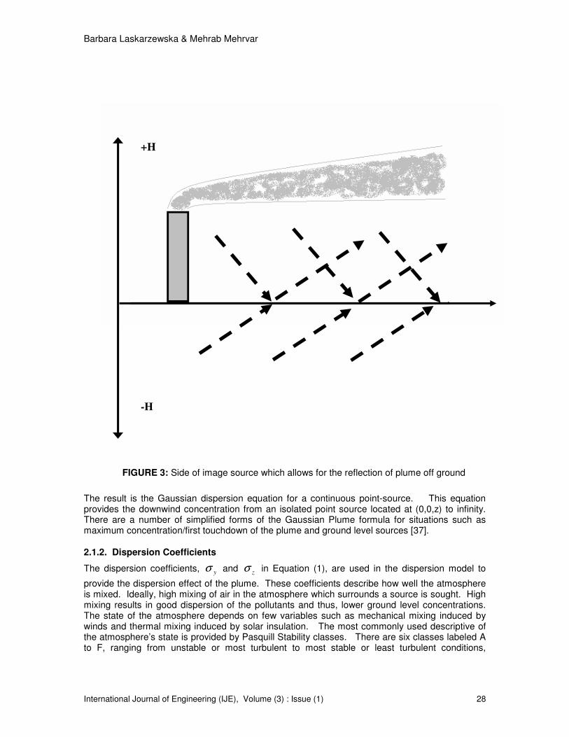
The basic Gaussian Plume model is for a point source, i.e., the tall stack in space that emits without set barrier. The ground level concentrations can be evaluated to infinity. At some point in time, the plume disperses in the vertical direction and touches the ground. The basic formula can be further modified to account for the plume reflection from the ground, considered a zero flux or impenetrable surface. This was accomplished by creating an image source component in basic Gaussian Plume formula, as shown in Equation (3).
( ) ( )
+−+
−−
−=
2
2
2
2
2
2
2exp
2exp
2exp
2),,(
zzyzy
p HzHzy
U
QzyxC
σσσσσπ (3)
The reflection source is shown in Figure 3.
FIGURE 2: Effective stack height of a point source is a sum of the stack height and plume rise. The momentum and thermal rise add up to the physical height of the stack
creating an effective stack height
z
wind
x
Height of the
Stack (Hs)
Plume Rise (∆H)
Barbara Laskarzewska & Mehrab Mehrvar
International Journal of Engineering (IJE), Volume (3) : Issue (1) 28
The result is the Gaussian dispersion equation for a continuous point-source. This equation provides the downwind concentration from an isolated point source located at (0,0,z) to infinity. There are a number of simplified forms of the Gaussian Plume formula for situations such as maximum concentration/first touchdown of the plume and ground level sources [37].
2.1.2. Dispersion Coefficients
The dispersion coefficients, yσ and zσ in Equation (1), are used in the dispersion model to
provide the dispersion effect of the plume. These coefficients describe how well the atmosphere is mixed. Ideally, high mixing of air in the atmosphere which surrounds a source is sought. High mixing results in good dispersion of the pollutants and thus, lower ground level concentrations. The state of the atmosphere depends on few variables such as mechanical mixing induced by winds and thermal mixing induced by solar insulation. The most commonly used descriptive of the atmosphere’s state is provided by Pasquill Stability classes. There are six classes labeled A to F, ranging from unstable or most turbulent to most stable or least turbulent conditions,
+H
-H
FIGURE 3: Side of image source which allows for the reflection of plume off ground

Barbara Laskarzewska & Mehrab Mehrvar
International Journal of Engineering (IJE), Volume (3) : Issue (1) 29
respectively [37]. Table 2 provides the Pasquill Stability classes which describe the state of the atmosphere. TABLE 2: Pasquill dispersion classes related to wind speed and insulation [37] (Adopted from Turner 1970)
Surface
Wind Speedd
Day Incoming Solar Radiationa,c
Night Cloudinessb,c
(m/s) Stronge Moderate
f Slight
g Cloudy Clear
<2 A A-B B - - 2-3 A-B B C E F 3-5 B B-C C D E 5-6 C C-D D D D >6 C D D D D
A. Insulation, incoming solar radiation: Strong > 143 cal/m2/sec, Moderate = 72-143 cal/m2/sec, Slight < 72 cal/m2/sec. b. Cloudiness is defined as the fraction of sky covered by clouds. c. A – very unstable, B – moderately unstable, C – slightly unstable, D – neutral, E – slightly stable, F – stable. Regardless of wind speed, Class D should be assumed for overcast conditions, day or night. d. Surface wind speed is measured at 10 m above the ground. e. Corresponds to clear summer day with sun higher than 600 above the horizon. f. Corresponds to a summer day with a few broken clouds, or a clear day with sun 35 – 600 above the horizon. g. Corresponds to a fall afternoon, or a cloudy summer day, or clear summer day with the sun 15 – 350.
The Pasquill dispersion coefficients are based on the field experimental data, flat terrain, and rural areas. The plots allow for the user to read off dispersion coefficient at specific distance for selected stability class extracted from Table 2. The graphical plots of the dispersion coefficients become useless when solving Gaussian dispersion using a box model on a computer platform. A number of analytical equations have been developed that express dispersion coefficients for rural and urban areas. These algebraic solutions are fitted against the dispersion coefficient plots and provide a few methods to calculate each dispersion factor. One of the methods is the use of power law to describe dispersion coefficients [37] and [40]:
σy = bax (4)
σz = ecxd +
where x and variables a through e are distance [m] and dimensionless parameters, respectively. Parameters a through e are functions of the atmospheric stability class and the downwind is a function to obtain dispersion coefficients or a combination of power law and another approach. Another approach, most commonly used in dispersion models is shown as follows [40]:
σy θtan15.2
=
x (5)
where ( )xgf ln−=θ and θ , f and g are angle [0] and two dimensionless parameters,
respectively. McMullen [41] developed the following dispersion coefficients as the most representative of Turner’s version of the rural Pasquill dispersion coefficients for rural areas. The advantage of the McMullen’s equation is its application to both vertical and horizontal dispersion coefficients.
( )2)(lnlnexp xixhg ++=σ (6)

Barbara Laskarzewska & Mehrab Mehrvar
International Journal of Engineering (IJE), Volume (3) : Issue (1) 30
Constants g through i are dimensionless parameters as provided in Table 3. There also exist
dispersion coefficients suitable for urban areas. Experimental data obtained from urban areas result in higher dispersion coefficients [42] and [43]. The plume encounters turbulence due to buildings and relatively warmer temperatures associated with urban areas. These can alter the atmospheric conditions for a small localized area when compared to the prevailing meteorological conditions. A higher dispersion coefficient results in a closer maximum ground-level concentrations as demonstrated in Figure 4.
TABLE 3: Constants g, h, and i in McMullen’s Equation (6) for rural dispersion coefficients [37]
To obtain σz To obtain σy Pasquill Stability
Class g h i g h i
A 6.035 2.1097 0.2770 5.357 0.8828 -0.0076 B 4.694 1.0629 0.0136 5.058 0.9024 -0.0096 C 4.110 0.9201 -0.0020 4.651 0.9181 -0.0076 D 3.414 0.7371 -0.0316 4.230 0.9222 -0.0087 E 3.057 0.6794 -0.0450 3.922 0.9222 -0.0064 F 2.621 0.6564 -0.0540 3.533 0.9191 -0.0070
FIGURE 4: Effect of urban and rural dispersion coefficients. For urban areas a higher maximum ground level concentration, i.e. Cmax(urban), is observed and closer to the source. For rural areas a
lower maximum ground level concentration, i.e. Cmax(rural), is observed and it occurs further from the source
For a plume passing through an urban area, the maximum ground-level concentration not only occurs closer to the source but also appears at a higher concentration than if modeled in rural area. In addition, further away from the urban area, a plume results in a lower ground level concentration than that if modeled in rural area. Initial mixing induced by the turbulence in a city
C
x
Higher σ values - urban
Lower σ values - rural C max (urban)
C max (rural)

Barbara Laskarzewska & Mehrab Mehrvar
International Journal of Engineering (IJE), Volume (3) : Issue (1) 31
W
W
W
W
2W
15.2
2Wyo =σ
results in a better dispersion. For urban areas, the dispersion coefficients can be expressed by previously mentioned power law, with corrected constants, as shown in the following equation:
( )lkxjx += 1σ (7)
Constants j through l are dimensionless parameters are provided in Table 4. There seems to not be a single better solution, therefore, when selecting a method, one should evaluate the various approaches [44].
TABLE 4: Constants j, k, and l for estimation of Briggs urban dispersion coefficients in Equation (7) [37]
To Obtain σz To Obtain σy Pasquill
Stability Class
j k l j k l
A-B 240 1.00 0.50 320 0.40 -0.50 C 200 0.00 0.00 220 0.40 -0.50 D 140 0.30 -0.50 160 0.40 -0.50
E-F 80 1.50 -0.50 110 0.40 -0.50
2.1.3. Characterization of Various Emission Sources in Gaussian Dispersion Model
The Gaussian Plume model originally developed for point sources (i.e. tall stacks) can be also applied to other types of emission sources. These emission sources are most commonly described as volume, line, and area sources. The box dispersion models are also capable of handling sources below grade and flares. These sources (e.g. quarries or flares) are not typical of Toronto city and therefore, will not be discussed. Toronto is mainly characterized by sky scrapers and highways, which can translate to volume sources and line (or area) sources.
Volume Source A building structure is characterized in an air dispersion model as a volume source. The solution proposed under the Gaussian Plume model is to model the volume source as a point source at a distance with matching dispersion coefficients to the dimensions of the virtual source [40], as shown in Figure 5. The initial lateral and vertical dimensions are modified dimensions of source width and height, as shown in Table 5.
1 2
1 2
15.2
2Wyo =σ

Barbara Laskarzewska & Mehrab Mehrvar
International Journal of Engineering (IJE), Volume (3) : Issue (1) 32
FIGURE 5: (Upper) Line source represented by adjacent volume source. (Lower) Line source represented
by separated volume source
TABLE 5: Initial dimensions for a virtual source [40]
Type of Source Procedure for Obtaining Initial Dimension
Initial Lateral Dimension ( yoσ )
Single Volume Source 3.4
Lyo =σ
Line Source Represented by Adjacent Volume Source (Figure 5) 15.2
Lyo =σ
Line Source Represented by Separate Volume Source (Figure 5) 15.2
Ayo =σ [ A – centre to centre distance]
Initial Vertical Dimension ( zoσ )
Surface-Based Source (H=0) 15.2
Bzo =σ [B – vertical dimension]
Elevated Source (H >0) on or Adjacent to Building 15.2
Czo =σ [C – building height]
Elevated Source (H>0) not on or Adjacent to a Building 3.4
Azo =σ
Line Source Line source is characterized by being a surface based source at grade-level. Road emissions
can be modeled as line sources. Figure 6 shows a line source of length L and strength
lQ normal to the wind vector. The emissions, lQ , arise from a small segment of a line, 'dy , and
are expressed as 'dyQl . The receptor is located at point ),( yx downwind of the line source.
One of the solutions to represent line sources by Gaussian Plume formula is given by [45].
+
+
−
=yyz
l
yL
erf
yL
erfU
QC
σσσπ 2
2
2
2
2 (8)
and are source strength [g/s] and length [m], respectively. This equation is used to estimate the concentration downwind of an infinite line source normal to the mean wind vector.

Barbara Laskarzewska & Mehrab Mehrvar
International Journal of Engineering (IJE), Volume (3) : Issue (1) 33
FIGURE 6: A line source of length L and strength lQ
The governing equation of a line source oriented at an oblique angle, as shown in Figure 7, to the
mean wind vector was developed by Calder [43]. The perpendicular distance, pd , is the distance
between the receptor and the line source. Angle θ is the angle between its normal and the wind vector and applies to angles as large as 75
o [46].
This solution is shown in Equation (9) [45]:
=
θθσ
π
coscos
2
p
z
l
dU
QC (9)
where pd is perpendicular distance [m]. A limitation of this approach includes its inability to
account for mixing due to heated exhaust [47].
x
y
+2
L
dy’
wind
y’
2
L−
R(x,y) y’-y
Line Source (Ql)

Barbara Laskarzewska & Mehrab Mehrvar
International Journal of Engineering (IJE), Volume (3) : Issue (1) 34
FIGURE 7: Infinite line source with strength lQ at an oblique angle (θ ) to the wind
Area Source An alternative method that can be used to model emissions from a road is by describing the road as area source. Open fields from which wind erosion occurs is another example of an area
source. In essence, a line source with width 1x normal to the wind direction can be used to
represent an area source as shown in Figure 8. The area source (considered to be long enough
to be infinite) is a sum of smaller line sources, each of strength dxQa ' per unit length, where
emission rate is aQ . There are two descriptions of area sources that follow the Gaussian Plume
model.
y
dp
2
L−
R (x, 0)
θ
Line Source ( lQ )
θ=900
θcos
pd
x

Barbara Laskarzewska & Mehrab Mehrvar
International Journal of Engineering (IJE), Volume (3) : Issue (1) 35
FIGURE 8: An area source with strength aQ and width 1x
In the case of area sources, dispersion coefficients are evaluated using power law as shown in Equation (10). The dispersion coefficient in the z-direction is to be evaluated for a distance of
xx − ' (concentration at a receptor) and thus, it is expressed in a power law form [45]:
( )n
z xxm '−=σ (10)
where ( xx − '), m, and n are distance [m] and two dimensionless parameters, respectively. Dimensionless parameters are a function of atmospheric stability and selected from Table 6.
TABLE 6: Power law constants used to calculate the dispersion coefficients in Equation (10) [45]
σya σz (0.5 – 5 km) σz (5 – 50 km) Dispersion Class a b m n m n
A 0.3658 0.9031 2.5× 10⁻⁴ 2.1250 - -
B 0.2751 0.9031 1.9× 10⁻³ 1.6021 - -
C 0.2089 0.9031 0.20 0.8543 0.5742 0.7160 D 0.1474 0.9031 0.30 0.6532 0.9605 0.5409 E 0.1046 0.9031 0.40 0.6021 2.1250 0.3979 F 0.0722 0.9031 0.20 0.6020 2.1820 0.3310
a Use power law mentioned previously to evaluate horizontal dispersion.
The following equation [45] is used to determine concentrations at receptor from a downwind
edge. The source height, H , allows one to utilize this approach to road sources where emissions are released at the above ground at the height of the truck.
y
R (x, 0)
dx’
x
Area Source ( aQ )
wind
x1

Barbara Laskarzewska & Mehrab Mehrvar
International Journal of Engineering (IJE), Volume (3) : Issue (1) 36
( )
∫∫=
+
−=
−
−−
=1
0'
2
2
2
2
2
2'
''22
'exp
x
x ZY
zy
L
Ly
a dydx
Hyy
U
QC
σσ
σσ
π (11)
where Qa and )'( yy − are strength of area source [g/m2/s] and distance [m], respectively,
)'( xxyY −= σσ and )'( xxzZ −= σσ . This solution is time consuming when evaluated
numerically, therefore, often an approximation developed by Calder [48] is used. This solution is called the narrow plume approximation as shown in Equation (12):
∫
−= −
1
0
2
21 '
2exp
2x
z
z
a dxH
U
QC
σσ
π (12)
where parameters are defined as before.
2.1.4. Limitations of Gaussian Plume Dispersion
There are a number of limitations that must be observed before applying the basic Gaussian Plume model to air dispersion problems. Following is a description of each limitation [37]:
a) vertical and crosswind diffusion occur according to Gaussian distribution; b) downwind diffusion is negligible compared to downwind transport;
c) the emissions rate, Q , is continuous and constant;
d) the horizontal wind velocity and the mean wind direction are constant; e) there is no deposition, washout, chemical conversion or absorption of emissions, and
any emissions diffusing to the ground are reflected back into the plume (i.e. all emissions are totally conserved within the plume);
f) there is no upper barrier to vertical diffusion and there is no crosswind diffusion barrier; g) emissions reflected upward from the ground are distributed vertically as if released
from an imaginary plume beneath the ground and are additive to the actual plume distribution; and
h) the use of yσ and zσ as constants at a given downwind distance and the
assumption of an expanding conical plume require homogeneous turbulence throughout the x , y and z -directions of the plume.
It is important to note that many of these limitations have been resolved by studies conducted in the application of Gaussian Plume dispersion model to urban areas. Additional limitations can arise in following situations, identified by this study, such as decision over election of source type (i.e. line, area or volume) adequate to be assigned to an emission source e.g. road sources. Another limitation of the model is its under performance during cooler months of the year. This can be potentially resolved through the modification of dispersion coefficients.
2.1.5. Chemistry in Gaussian Plume Dispersion
One of the most commonly used Gaussian Plume model is ISC-PRIME. [49][31][32][36] This box model handles NOx and SOx in following ways:
a) decay term; b) dry deposition; and c) wet deposition.
The use of decay term D [s-1] is one way of including the removal of a pollutant in the Gaussian
Plume model as follows [40]:
( ) ( )
+−+
−−
−=
2
2
2
2
2
2
2exp
2exp
2exp
2),,(
zzyzy
p HzHzy
U
DQzyxC
σσσσσπ (13)
Barbara Laskarzewska & Mehrab Mehrvar
International Journal of Engineering (IJE), Volume (3) : Issue (1) 37
where D is decay term [s-1
]. The decay term in the ISC-PRIME model is defined as follow:
−=
U
xD ψexp (14)
where
2/1
693.0
T=ψ and 2/1T is the pollutant half life (s
-1) [50].
Furthermore, the box model utilizes a decay term of 4.81×10⁻⁵
s-1
for SO2 concentrations when modeled in urban area. There is no similar decay term assigned to NOx pollutant in this box model [40].
There also exists a dry deposition option available in the box model ISC-PRIME. It is applied to particulate formed by gaseous pollutants. These emissions are characterized by a high fraction
of particulate over 2 µm in diameter. The following approach estimates deposition velocity and must be evaluated for each mass fraction and each particle category [51].
( )ggdadad vvrrrrv +++=
−1 (15)
where dad rr ,,ν , and gν are deposition velocity [cm/s], aerodynamic resistance [s/cm], deposition
layer resistance [s/cm], and gravitational settling velocity [cm/s], respectively. The distance closer to the ground can be divided into two phases:
a) fully turbulent region with vertical fluxes constant; b) a thick quasi-laminar sub-layer.
Both regions can be identified using Monin-Obukhov length, L , an implicit function of friction
velocity. Iteration is used to evaluate L until the solution converges [51]. The iteration is completed using Equation (16):
Ψ+
Ψ−
=
L
z
L
z
z
z
kuu
m
ref
m
ref
ref
0
0
*
ln
(16)
where:
2tan2
2
1ln
2
1ln2 1
2 πµ
µµ+−
++
+=
Ψ −
L
zref
m
4
1
161
−=
L
zrefµ
2tan2
2
1ln
2
1ln2 0
1
2
000 πµ
µµ+−
++
+=
Ψ −
L
zm
4
1
0161
−=
L
zµ
kgH
uTcL
refp
3
*ρ−=
In the above equations, Lukzzu refref ,,,,, 0* , and mΨ are surface friction velocity [cm/s],
reference elevation [m], elevation [m], surface roughness length [m], unit-less von Karman constant [0.40], wind speed at reference elevation [m/s], Monin-Obukhov length [m], and decay
coefficient [s-1
], respectively. Also, refp Tc ,,, ρµ , and g are absolute viscosity of air

Barbara Laskarzewska & Mehrab Mehrvar
International Journal of Engineering (IJE), Volume (3) : Issue (1) 38
[41081.1 −× g/cm/s], particle density [g/cm
3], specific heat of air at a constant pressure, reference
temperature [K], and acceleration due to gravity [cm/s2], respectively.
For the turbulent region, the dominant is the aerodynamic resistance. For the turbulent region following equation applies, where L is > 0:
+
=
L
z
z
z
kur
o
d
a 7.4ln1
*
(17)
For L <0, the following equation applies:
−
+
+
+
+
+
−
+
=
11611161
11611161
ln1
0
0
0
*
L
z
L
z
L
z
L
z
kura
(18)
where *u , dz , and 0L are surface friction velocity [cm/s], surface roughness [m] and initial length
[m], respectively. A minimum value of 1 m for Monin-Obukhov lengths is assumed for rural locations. The deposition layer resistance is expressed as:
*
3
3
2
10
1
uSc
r
St
d
+
=−−
(19)
where cS and tS are Schmidt and Stokes numbers, respectively.
The Schmidt number has an impact on the deposition rate of small particles, particles that follow Brownian motion. The parameter with the Stokes number is a measure of inertial impact,
dominated by intermediate sized particles (2-20 µm). [51] The gravitational settling velocity is expressed as:
( )CF
pair
g Scgd
µ
ρρν
18
2
2−= (20)
where 2,,,, cdv pairg ρρ , and CFS are gravitational settling velocity [cm/s], particle density
[g/cm3], air density [
3102.1 −× g/cm3], particle diameter [µm], air units conversion constant
[8101 −× cm
2/µm
2], and dimensionless slip correction factor, respectively. Finally the slip factor
can be estimated as follow:
p
p
CFd
x
daaax
S4
2
3212
10
exp2
1−
−+
+= (21)
where 2x , 1a , 2a , and 3a are all dimensionless constants [6.5× ,10 6− 1.257, 0.4, and
0.55× 410−, respectively]. A user of a box model who wishes to utilize acid rain can accomplish
it by use of wet deposition syntax. The settling velocity and a product of the concentration as expressed in Equation (3) give dry deposition [40]:
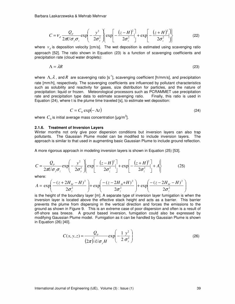
Barbara Laskarzewska & Mehrab Mehrvar
International Journal of Engineering (IJE), Volume (3) : Issue (1) 39
( ) ( )
+−+
−−
−=
2
2
2
2
2
2
2exp
2exp
2exp
2 zzyzy
p
d
HzHzy
U
QC
σσσσσπν (22)
where dv is deposition velocity [cm/s]. The wet deposition is estimated using scavenging ratio
approach [52]. The ratio shown in Equation (23) is a function of scavenging coefficients and precipitation rate (cloud water droplets):
Rλ=Λ (23)
where λ,Λ , and R are scavenging ratio [s-1
], scavenging coefficient [h/mm/s], and precipitation
rate [mm/h], respectively. The scavenging coefficients are influenced by pollutant characteristics such as solubility and reactivity for gases, size distribution for particles, and the nature of precipitation: liquid or frozen. Meteorological processors such as PCRAMMET use precipitation rate and precipitation type data to estimate scavenging ratio. Finally, this ratio is used in Equation (24), where t is the plume time traveled [s], to estimate wet deposition:
( )tCC Λ−= exp0 (24)
where 0C is initial average mass concentration [µg/m3].
2.1.6. Treatment of Inversion Layers Winter months not only give poor dispersion conditions but inversion layers can also trap pollutants. The Gaussian Plume model can be modified to include inversion layers. The approach is similar to that used in augmenting basic Gaussian Plume to include ground reflection.
A more rigorous approach in modeling inversion layers is shown in Equation (25) [53].
( ) ( )
+
+−+
−−
−= A
HzHzy
U
QC
zzyzy
p
2
2
2
2
2
2
2exp
2exp
2exp
2 σσσσσπ (25)
where:
=A
−−−+
+−−+
−+−2
2
2
2
2
2
2
)2(exp
2
)2(exp
2
)2(exp
z
bl
z
bl
z
bl HHzHHzHHz
σσσ
is the height of the boundary layer [m]. A separate type of inversion layer fumigation is when the inversion layer is located above the effective stack height and acts as a barrier. This barrier prevents the plume from dispersing in the vertical direction and forces the emissions to the ground as shown in Figure 9. This is an extreme case of poor dispersion and often is a result of off-shore sea breeze. A ground based inversion, fumigation could also be expressed by modifying Gaussian Plume model. Fumigation as it can be handled by Gaussian Plume is shown in Equation (26) [40].
( )
−=
2
2
2
12
1exp
2
),,(y
y
p y
HU
QzyxC
σσπ (26)

Barbara Laskarzewska & Mehrab Mehrvar
International Journal of Engineering (IJE), Volume (3) : Issue (1) 40
z
Inversion layer
Effective stack height
x
FIGURE 9: Fumigation induced by an inversion layer located above the effective stack height. The inversion layer acts similar to a mirror sealing and forces the plume to the group which
result in poor dispersion and higher maximum ground level concentrations at the ground level
There are a number of other inversion layers and some assist the dispersion. Lofting is a reverse of fumigation as shown in Figure 9 [54]. The inversion layer is located below the top of the stack and therefore, forces the plume to disperse in the upward direction [50].
3. ATMOSPERHIC CHEMISTRY OF NOx AND SOx
In an urban area, the main sources of NOx and SOx emissions arise from the road traffic, emissions from fuel fired equipment which provides power/electricity, and fuel fired equipment which provides power/electricity, and industries. At the present time, the most complete databases (i.e. National Pollutant Release Inventory (NPRI)) available in Canada contain the emissions of NOx and SOx from industrial sources only. Most recent publication shows that transportation contributes to 40% of NOx (transportation) and 28% NOx (road vehicles) and 4% SOx (transportation) annually [55]. Emissions of NOx into the atmosphere due to combustion of fuel are driven by the nitrogen in the atmosphere. Approximately 90% of emissions due to combustion of fuel result in NO [53]. NO can potentially convert to NO2, therefore, it is often referred to as NOx and NO2 when estimating emissions. In addition, for urban areas, diurnal variations in NOx are observed due to morning and afternoon traffics. Emissions of SOx into the

Barbara Laskarzewska & Mehrab Mehrvar
International Journal of Engineering (IJE), Volume (3) : Issue (1) 41
atmosphere due to combustion of fuel are strictly related to sulphur content in the fuel. Regulations are put in place to control the content of sulphur in fuel, result for the annual and diurnal cycles to be significantly reduced in comparison to that of NOx [56]. There are a number of deposition mechanisms that can be identified with NOx and SO2 such as dry deposition, wet deposition, and cloud water deposition. These mechanisms are discussed in the following with means to further augment existing Gaussian Plume model.
3.1. Dry Deposition The surface concentration always tends towards the atmospheric concentration. This tendency can be disrupted by three processes which move the gasses down the gradient between the atmosphere and the surface. Turbulent diffusion moves the gas to the surface. Molecular diffusion transfers the gas across the laminar boundary layer next to the surface. Gas molecules dissolve or react with the surface itself. All three must be present for dry deposition to occur. Dry deposition is a function of deposition velocity and the transfer resistance. Formation of sulphuric acid and nitric acid are two dry reactions of importance to emissions from urban areas. Some measurements of dispersing plumes show a 4% per hour, on a sunny day for the conversion of SO2 to H2SO4 [53]. Production of nitric acid occurs at night as the radical is photolytically unstable. Deposition Velocity Given there is a flux due to a gradient between the atmospheric concentration at 1-2 m above the ground and zero concentration at the surface, the deposition velocity is given as [57]:
z
g
gC
Fv = (27)
Where gv , gF , and zC are deposition velocity [m/s], flux to surface [kg/m2/s] and atmospheric
concentration [kg/m3], respectively [53]. The concentration in Equation (27) is evaluated at known height, z. Transfer Resistance Transfer resistance is considered as a part of the concept of conductance to describe particulate deposition from atmosphere to surface. Deposition velocity is defined as conductance.
g
tv
r1
= (28)
Where tr is the total transfer resistance [s/m]. Total resistance is calculated using Equations (28)
and (29), and incorporating ground level concentration:
sasurfacerain
g
S
g
Sz rrrrF
C
F
CCr +=+=+
−= (29)
Where r , zC , sC , gF , ar , and sr are resistance [s/m], atmospheric concentration [kg/m3] at
reference height, surface concentration [kg/m3], flux to surface [kg/m
2/s], aerodynamic resistance
[s/m], and surface resistance [m/s], respectively. The aerodynamic resistance, ar , can be added
as two resistors in series: turbulent resistance transfer and by eddies and molecular diffusion of the gas through the laminar boundary layer to the surface itself. For urban area, an area with high surface roughness and strong winds, the aerodynamic resistance becomes low. Table 7
summarizes typical aerodynamic values used for ar . The surface resistance values have been
widely studied and are readily available [57].
TABLE 7: Typical aerodynamic resistance values (ra) for various wind speeds and vegetation [53]

Barbara Laskarzewska & Mehrab Mehrvar
International Journal of Engineering (IJE), Volume (3) : Issue (1) 42
Aerodynamic Resistance (ra)
[s/m] Condition
200 Wind speed < 1 m/s, vegetation 10 cm tall
20 Wind speeds > 4 m/s, over 1 m vegetation 20 Wind speeds of < 10 m/s, forest canopy
The resistances that related to stomata: deposition to dry leaf surface, deposition to liquid water on leaf surface and deposition to the soil, are additional paths that might be considered. Each
path having its own resistance component adds to the equation. Suggested values of gν are
10 mm/s during the day time and 5 mm/s at night for NO2 and SO2 [57].
Dry deposition, Equation (29), was expanded by Wesely [58] for SO2. This equation is
augmented to include a term which represents bulk surface resistance, cr . The cr includes not
only vegetated surfaces but the range of surface conditions. Bulk surface resistance for seasonal categories and land use may be estimated using equation augmented in Equation 29. As the temperature drops (< -2
oC), the surface resistance increases. Therefore, Wesely [58] briefly
discussed surface uptake of HNO3, SO2, and NO2 by the following term for each substance.
Surface Uptake =( )4
1000+− ST
e (30)
where ST is the surface temperature [K].
3.2. Wet Deposition
Sulphur and nitrogen are incorporated into cloud droplets, raindrops and snow flakes, which are deposited on ground. The reactions of sulphur and nitrogen in water form a complex set based on presence of gaseous O3 and H2O2, and catalysts Mn and Fe at surface of aerosol particles. These reactions last for days, thus deposition may occur thousand kilometers from the source [53].
3.3. Cloud Water Deposition
Scavenging below and in-cloud of gases is yet another transport phenomenon which should be accounted for in air dispersion models. The SO2 gas can dissolve in clouds as it is considered a moderately soluble gas [59].
One approach to estimate below-cloud scavenging is proposed by Asman [59]. The equations are limited to rain and do not include “snow” type of precipitation. Below cloud scavenging
coefficient, bΛ , is a function of rain fall, I, as described in Equation (31). Temperature, )0(aT ,
and relative humidity, rh (0), are measured at ground level.
avb
mmb aI=Λ (31)
where:
)15.1298(gbbDaaa +=
)0(10 rhaaaa +=
)0(10 rhbbbb +=
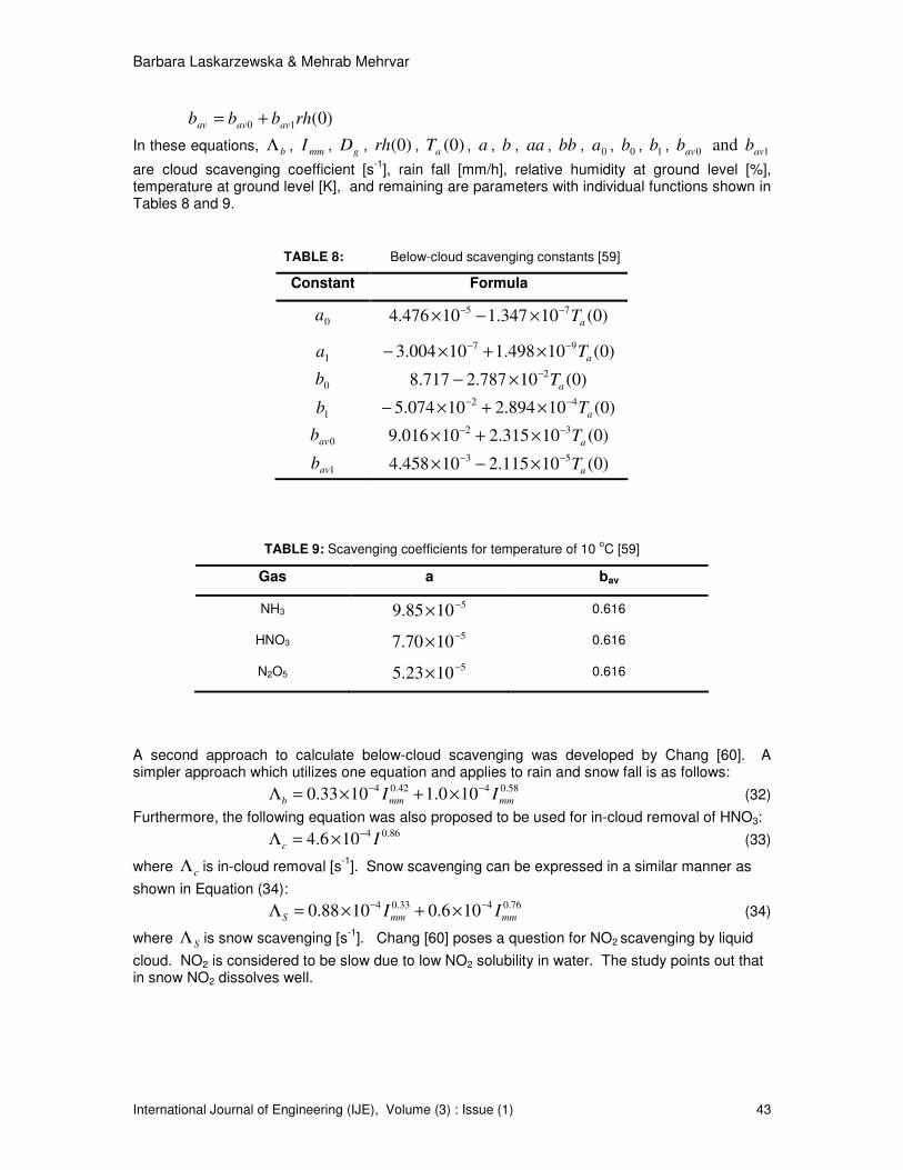
Barbara Laskarzewska & Mehrab Mehrvar
International Journal of Engineering (IJE), Volume (3) : Issue (1) 43
)0(10 rhbbb avavav +=
In these equations, bΛ , mmI , gD , )0(rh , )0(aT , a , b , aa , bb , 0a , 0b , 1b , 0avb and 1avb
are cloud scavenging coefficient [s-1
], rain fall [mm/h], relative humidity at ground level [%], temperature at ground level [K], and remaining are parameters with individual functions shown in Tables 8 and 9.
TABLE 8: Below-cloud scavenging constants [59]
Constant Formula
0a
)0(10347.110476.4 75
aT−− ×−×
1a
)0(10498.110004.3 97
aT−− ×+×−
0b
)0(10787.2717.8 2
aT−×−
1b
)0(10894.210074.5 42
aT−− ×+×−
0avb
)0(10315.210016.9 32
aT−− ×+×
1avb
)0(10115.210458.4 53
aT−− ×−×
TABLE 9: Scavenging coefficients for temperature of 10 oC [59]
Gas a bav
NH3 51085.9 −× 0.616
HNO3 51070.7 −× 0.616
N2O5 51023.5 −× 0.616
A second approach to calculate below-cloud scavenging was developed by Chang [60]. A simpler approach which utilizes one equation and applies to rain and snow fall is as follows:
58.0442.04 100.11033.0 mmmmb II−− ×+×=Λ (32)
Furthermore, the following equation was also proposed to be used for in-cloud removal of HNO3: 86.04106.4 Ic
−×=Λ (33)
where cΛ is in-cloud removal [s-1
]. Snow scavenging can be expressed in a similar manner as
shown in Equation (34): 76.0433.04 106.01088.0 mmmmS II
−− ×+×=Λ (34)
where SΛ is snow scavenging [s-1
]. Chang [60] poses a question for NO2 scavenging by liquid
cloud. NO2 is considered to be slow due to low NO2 solubility in water. The study points out that in snow NO2 dissolves well.

Barbara Laskarzewska & Mehrab Mehrvar
International Journal of Engineering (IJE), Volume (3) : Issue (1) 44
4. APPLICATIONS OF GAUSSIAN PLUME MODEL TO URBAN AREAS
The evaluation of emissions for an urban area depends on emission summary, meteorological data, and surroundings. This information can be embedded into a dispersion model to estimate concentrations of various chemicals across the area of interest. The predicted concentrations can further be compared to the monitored data of the area. There are a number of approaches applied to dispersion of pollutants around a city which include the study of street canyons, forecasting type of modeling, and applications of statistical distribution to describe behaviour of a plume. This section evaluates the applications of Gaussian dispersion to five cities around the world and provides a critique of different applications of Gaussian dispersion for urban areas. Two studies have been completed on predicting ground level concentrations of various pollutants for the City of Toronto, one using land use regression and second a Gaussian dispersion model. The final subsection contains a description of a small scale study conducted for the city of Toronto, Ontario, Canada, and emissions due to traffic specifically emissions of NO2. The ground level concentrations were predicted using ISC-PRIME model and compared to the monitored data. The dispersion modeling was conducted for the first few days of February 2005, days leading to the earliest smog season recorded in Toronto [12]. 4.1. Dispersion Modeling of the City of Kanto, Japan Kitabayashi et al. [4] studied NOx emissions for a mega city, Kanto, Japan. The main sources included mobile sources (trucks), an electric power plant, and ventilation towers that service automotive tunnels. In that study, the Gaussian plume model was augmented with a chemical reaction module and incorporated concentrations for background gases. The integrated model was tested against a typical stack gas (point source). Results were stated as reliable with no analysis provided. This would quantify the relationship of data that led to a conclusion of the model’s reliability. Proposed investigations for the future include inclusion of more data (i.e. monitoring stations) for the area of interest and comparison of observed concentrations to the predicted by the integrated Gaussian plume model.
The above model lacks statistical analysis in the form of comparing percentiles of modeled concentrations to monitored data for different time frames. The study overcomes one of the Gaussian dispersion limitations: the equation of continuity assumes dispersion of a chemically stable material that did not deposit to the ground [53]. The model could be augmented by the addition of dry and wet deposition for the NOx and SOx species using methods described in the open literature [61], [62], [63] and [64]; thus, improving the overall mass balance.
4.2. Dispersion Modeling of the City of London, UK
Two dispersion models were studied for the city of London, UK. First Model Owen et al. [5] utilized an existing air dispersion model which incorporated skewed – Gaussian distribution, ADMS-URBAN, along with meteorological data from one meteorological station, background concentrations of pollutants of interest for the 1995, year and emissions inventory from 1997 for the city of London. The model covered a domain of approximately 40 km by 40 km in the city of London and estimated ground level concentrations of NOx and NO2. The main sources of emissions (75 wt%) were roads characterized as line sources and industrial sources characterized as point sources.
The modeled concentrations were compared to the monitored data for the summer and winter of 1995. Concentrations of NOx and NO2 were predicted utilizing the empirical function derived by Derwent and Middleton [65]. The modeled concentrations showed an under-prediction for winter months with a conclusion that the overall model’s performance was reasonable when compared to the monitored data.

Barbara Laskarzewska & Mehrab Mehrvar
International Journal of Engineering (IJE), Volume (3) : Issue (1) 45
For the predicted occurrences of the highest concentrations, the meteorological data during the winter season was reviewed and reasons for possible under predictions were provided. The under prediction in the cooler season was due to (cold stable conditions) the poor dispersion. In addition, the average daily traffic flow was used while the remaining information was set in the model on an hourly basis. The cold stable conditions may be described by using the approach of Milliez and Carissimo [66] and Owen et al. [5] commented on missed smaller sources (i.e. winter emissions due to combustion related to heating of homes). Perhaps if hourly data of traffic were available, the correlation would have been improved.
The study did include review of modeled concentrations for the top percentiles against the observed data. The statistical analysis included the calculation of mean, standard deviation, correlation, and fraction of data within a factor of two.
A description of the model setup and grid density, chemistry, building effect and dry and wet deposition was not discussed in the above model. The chemistry may be approached using methods of Asman, Chang, Wesely and Cana-Cascallar [59], [60], [58] and [67]. The building effect on the dispersion and modification to the dispersion code can be set as per any of the proposed solutions by Milliez and Carissimo, Xie et al., Baker et al., Baik et al. [66], [68], [69] and [70]. Treatment of slow winds may be approached by the method used by Goyal et al. [71]. All these approaches would have been refined the algorithm and possibly lead to a better correlation. The study did not also comment on the use of various years for input into the model. Obtaining input data and meteorological information for the same year as the observed ambient concentrations would yield refined correlations.
Second Model Seika et al. [6] transformed the German dispersion model IMMAUS designed for the former city of west-Berlin into a computer platform formulated for the city of London, UK. The emission inventory included traffic, non traffic point, and area sources. Concentrations were evaluated on a gird of various densities from 1 to 10 km spatial separation. The model included hourly meteorological data and background concentrations. The Gaussian plume included total reflection. The dispersion model handled dry and wet deposition for area sources only. The modeled concentrations showed a good agreement to the monitored data observed for the year 1993.
The study also provided an in depth review of the physics behind the assumed dispersion, meteorology, and emissions inventory. An observed limitation was the need to improve how the Gaussian plume diffusion applied to wind speeds below 1 m/s, varying wind speeds and need a module which calculated mid-day boundary layer depths. The dry deposition for area sources
was simulated using Chamberlain’s source depletion formulation. The study did not provide statistical analysis of the comparison for the modeled concentrations and observed values.
4.3. Dispersion Modeling of the City of Helsinki, Finland The NOx emissions, dispersion, and chemical transformation for Helsinki metropolitan area was also modeled by Karppinen et al. [7] and [8]. Its objective was to study traffic-originated NOx and to compare the results to four local monitoring stations for the year 1993. The domain of the city of Helsinki is approximately 30 by 30 km. Concentrations were modeled on a receptor grid with a network having dense grid (50 by 50 m) in the vicinity of the major roads and largest grid interval of 500 by 500 m around the perimeter of the city. Results were plotted as iso-concentration curves. The hourly traffic emissions were based on EEME/2 transportation planning system (INRO 1994) and new emission factors that related to Helsinki city traffic. Pollutant concentrations were computed using the road network dispersion model CAR-FMI and urban dispersion modeling system UDM-FMI. Road sources were modeled as line source and remaining sources were

Barbara Laskarzewska & Mehrab Mehrvar
International Journal of Engineering (IJE), Volume (3) : Issue (1) 46
assigned characteristics of point sources. The meteorological data was obtained from two YTV meteorological stations and the mixing height of the atmospheric boundary layer was evaluated from a sounding station 90 km North-West of the city.
The 1998 study compared predicted annual average concentration to the observed data, showing a good agreement. There was a good agreement between the modeled data and three of the 4 YTV stations, however, there was a poor agreement with the 4th station. Road emissions contributed less than 50% of total emissions. Their analysis showed traffic sources have greater effect than industrial sources on the ground-level concentrations. In another study [8], the evaluation of seasonal and monthly concentrations was included. The results still contain severe under prediction of the modeled NOx for the same 4th monitoring station as identified in the 1998 study. Furthermore, within the later study, the under prediction has been recognized for the winter months [8].
That study, comments on the variation between the modeled and observed concentrations. The statistical analysis included root mean squared error, index of agreement, correlation coefficient, normalized mean square error, and fractional bias. These parameters were applied to predicted and observed data sets as suggested by Willmott [38].
Both studies did not provide a review of all data provided by external bodies (meteorology, traffic, and ambient concentrations) utilized. The review of meteorology (i.e. wind roses, wind speeds, and stability classes) could provide an insight into variables that drive dispersion. Review of the calms and the treatment of calm conditions were not addressed. The study did not discuss traffic data to asses its limitations in the analysis. The review of ambient concentrations can give an insight of sampling methods and their limitations. Finally, the study did not address review data that did not pass quality control and thus, was not included in the modeling. Furthermore, Karppinen et al. [8] proceeded to compare modeled hourly average concentrations to the observed data. A discussion was not given on the shortcomings of the data. The hourly average concentrations did not have a good agreement with the monitored data. A preferred approach can include a review of more than 1 year of modeled, selecting a year that best represents the meteorological conditions. A further look at the hourly averages on a daily basis along with the review of the meteorological conditions for these hours and traffic data may have provided an insight into why certain hourly averages did not match the modeled values (e.g. reduced traffic due to shutdown of a street would have resulted in lower observed concentrations but was not seen by the model). The monitored data was obtained at 4 m for two stations and 6 m for the fourth station. The study did not specify at what heights the concentrations were predicted and if those heights relate to the monitored data. The study commented on road emissions being below 50% of the total emission and having a great impact on the final concentrations. It did not provide an explanation for this observation and it can be explained by source characteristics. Roads modeled as area sources are ground based and therefore, do not disperse as well as tall sources which have thermal and momentum rise (i.e. industrial sources). Tall sources, even though made more than 50% of the total emissions, disperse better than sources which behave as ground based sources. [40], [53], [37] and [45] In addition, road sources could have also been modeled as smaller virtual sources (i.e. width/length) as proposed in US EPA [51]. This approach is time consuming but addresses the dispersion associated with the traffic.
The lack of agreement between the modeled concentrations and the observed data at the 4th monitoring station may be explained by building downwash effect. The severe under prediction could be explained by a possible plume trap (i.e. busy intersection with tall buildings) around the area thus, resulting in higher observed concentrations. By reviewing the traffic data and locations of the monitoring stations, adjustments could have been made to correct the study to account for a better representation of the dispersion around the 4th monitoring station.
Barbara Laskarzewska & Mehrab Mehrvar
International Journal of Engineering (IJE), Volume (3) : Issue (1) 47
4.4. Dispersion Modeling of the City of Prague, Czech Republic Brechler [9] developed a Gaussian dispersion model for the city of Prague. Sources were characterized as point (stacks of thermal power plants), line (traffic sources), and area sources (cross roads, petrol stations, parking sites, railway, and bust stations). Emissions due to furnaces which heat homes were included. Brigg’s formula was used to define plume rise [72]. A complex network of monitors maintained by Czech Hydrometeorological Institute and hygienic service of the Prague city includes 27 monitors. The model was used to estimate concentrations of various pollutants for years 1994, 1996, and 1998.
The study did not explain the selection of non-consecutive years for which concentrations were evaluated. The model did resolve a limitation of a Gaussian dispersion model, inability to resolve flow field due to complex terrain. This was resolved by dividing the domain into smaller segments with individual meteorological conditions computed by a mesoscale model. Gaussian dispersion was selected primarily due to time limitations and simplicity of the model. An alternative approach to describing stability of the atmosphere was done by utilizing Bubnik – Koldovsky classification and not Pasquill [73]. This approach uses a classification based on the value of vertical gradient of temperature and splits all possible conditions of vertical temperature stability into 5 categories for each vertical segment. Pasquill-Gifford approach utilized solar insulation and wind speed [37]. The study did not discuss statistical analysis of the predicted values and monitored data.
4.5. Historical Work Completed on the Simulation of Pollution Type of Studies Completed for the City of Toronto, Canada
Remarkably, little work has been published on simulating ground level concentrations of various pollutants for the City of Toronto [74], [75] and [76] All three studies look at the emissions from the city using various tools and on various domain sizes.
First Study The 1996 publication by Lin et al. was a study of a single poor air quality episode observed on April 6, 1992, at some distance away from the City of Toronto. This publication was a result of a program entitled Southern Ontario Oxidants Study (SONTOS 92). The objective of the SONTOS 92 program was to study the impact of emissions from the City of Toronto on the ozone levels in two areas: the first one located 140 km North-East of the City of Toronto in the city of Hastings and the second one 80 km South-West of Toronto in the city of Binbrook. Lin et al. [74] applied a one dimensional photochemical transport model along with Lagrangian calculations to model the emission of pollutants from the city. The City of Toronto was assumed to be a box of 20 by 30 km. The model predicted concentrations of various contaminants in Hastings and compared them to the observed data on April 6, 1992. The study concludes that the City of Toronto has an impact on the ozone levels downwind and further studies on regional scale were to be completed. No results were published for the city of Binbrook. It is important to note that no other results or analysis of data collected under SONTOS 92 have been published.
Second Study Yang et al. [75] conducted a smaller in domain exercise by looking at pollution around a specific intersection located in the core of the City of Toronto at Bay Street and King Street. The study concentrated on the street canyon effect, similar to CFD type of exercises. This study was designed with a dense grid and included an area with very tall buildings (i.e. 330 m above grade). A non-steady state dispersion model (CALPUFF) was used to predict concentrations at the ground level and at various heights above grade. The meteorological data was predicted using MM5-a prognostic model. This publication did not study any particular air quality event that occurred in the city and did not compare results to measured data. The study concluded that CALPUFF is a potentially adequate tool which can simulate flow fields.

Barbara Laskarzewska & Mehrab Mehrvar
International Journal of Engineering (IJE), Volume (3) : Issue (1) 48
Third Study Unlike the two previous mentioned studies by which dispersion models were utilized, the study conducted by Jerrett et al. considered traffic pollution in the City of Toronto and utilized a land use regression (LUR) approach to predict ground level concentrations of NO2. The study was conducted in 2002 for a period of 2 weeks with numerous air samplers deployed across the City of Toronto. A regression of 0.69 was determined with the intention to include other sources and meteorological data to improve the results. In addition, the authors propose to generate more data to encompass a full year.
4.6. Preliminary Dispersion Modeling of the City of Toronto, Canada
In our own study, the Gaussian dispersion model along with local meteorological data was applied to road network with the objective to predict 1-h ground level concentrations of NO2. Furthermore, the objective of this study was to compare the predicted concentrations to those recorded by a local monitoring station. Description of the Event and Modeling Domain The timing of study was selected to be the first few days of February 2005, coinciding with the beginning of the earliest episode of smog recorded in Toronto. The area of study was selected to be two blocks of major streets surrounding a monitoring station located at Finch Avenue and Yonge Street, station I.D. 34020 [77], an approximate area of 36 km
2. The monitoring station did
not capture full data for the entire smog episode. The 1-h concentrations of SO2, NO2, NOx, PM2.5
and O3 observed at the monitoring station could be obtained from the historical depository [77]. The hourly meteorological data were obtained from a meteorological station at Toronto’s Lester B. Pearson International Airport [78], approximately 30 km away from the selected area of study shown in Figure 10. The meteorological data was collected 10 m above the ground. For the time under consideration, there were two predominant wind directions, with the winds occurring at 2 m/s from south-south-east and at 5.7 m/s from north-north-west, shown in Figure 11. Morning and afternoon peak-traffic times were modeled to occur from 7 am to 9 am and from 4 pm to 6 pm, respectively. Traffic data from 2001 [79] and the Environment Canada’s emission factors [80] for various vehicles were used to estimate emission rates of NO2.
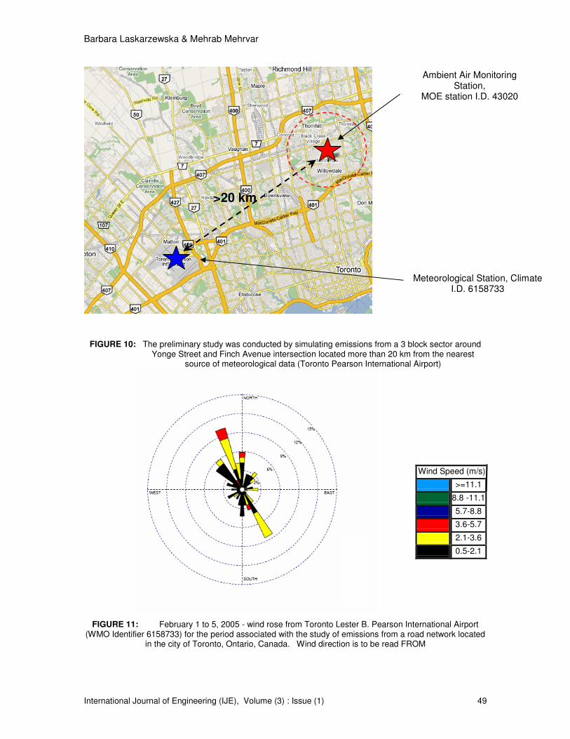
Barbara Laskarzewska & Mehrab Mehrvar
International Journal of Engineering (IJE), Volume (3) : Issue (1) 49
FIGURE 10: The preliminary study was conducted by simulating emissions from a 3 block sector around Yonge Street and Finch Avenue intersection located more than 20 km from the nearest
source of meteorological data (Toronto Pearson International Airport)
FIGURE 11: February 1 to 5, 2005 - wind rose from Toronto Lester B. Pearson International Airport (WMO Identifier 6158733) for the period associated with the study of emissions from a road network located
in the city of Toronto, Ontario, Canada. Wind direction is to be read FROM
Wind Speed (m/s)
>=11.1
8.8 -11.1
5.7-8.8
3.6-5.7
2.1-3.6
0.5-2.1
>20 km
Ambient Air Monitoring Station,
MOE station I.D. 43020
Meteorological Station, Climate I.D. 6158733

Barbara Laskarzewska & Mehrab Mehrvar
International Journal of Engineering (IJE), Volume (3) : Issue (1) 50
Finch Avenue
Bayview Avenue
Yonge Street Sheppard Avenue
Steels Avenue
Dispersion Model Setup The study area, shown in Figure 12, was set in ISC-PRIME dispersion model (version 04269) to evaluate 1-h ground level concentrations of NOx in urban area. Selection of urban option allowed for the model to utilize urban dispersion factors.
FIGURE 12: Area of study located in the city of Toronto, Canada, and modeled contour plots of ground
level concentrations, NOx µg/m3 (4 pm, February 4, 2005)
The characterization of road within the dispersion model was based on three options: as line been studied as potential methods to characterize road emissions within the Gaussian dispersion model. The limitation of a line source as mentioned earlier arises when winds approach at angles greater then 75
o. The area source has a limit on the length to width ratio 10:1. Furthermore, the
use of line or area sources yields an over prediction of the ground level concentrations [81] therefore, it was not evaluated in this study. A third option of setting up a road in a Gaussian dispersion model is to use numerous volume sources along the stretch of the path that follows road [51]. Sometimes this method is referred to as “equivalent line” source where the width of the
Ambient air monitoring station MOE I.D. 43020
Road segment

Barbara Laskarzewska & Mehrab Mehrvar
International Journal of Engineering (IJE), Volume (3) : Issue (1) 51
road becomes the basis for the initial lateral dimension. Inclusion of the plume spread factors allows to account for the mixing due to the elevated temperature of the exhaust gas [82]. In addition, each virtual source is separated by the width of the road (25 m) resulting in a series of volume sources. The height of the mobile equipment present on the road (3 m) was used to define the initial vertical dimension. The use of a volume source with embedded dispersion
factors ),( zy σσ allows the code to account for vehicle induced turbulence.
Results and Discussion The modeled and monitored concentrations for the peak traffic times between 7 am and 9 am are provided in Table 10. Preliminary statistical analysis summarized in Table 11 shows a good agreement between predicted and measured data. Plot of monitored data versus observed data yields a regression of 0.5. It was observed that both the morning and afternoon of day 1 had the least correlation. Note, the sample size is relatively small and further work is required to increase it.
TABLE 10: Summary of morning and afternoon peak time average concentrations of NO2 for the City of Toronto obtained in this study
Concentration (µg/m3) Day 1 Day 2 Day 3 Day 4 Remarks
Morning
Monitoring Station
I.D. 43020 79 88 81 120
Results from the
Simulation in ISC-PRIME 55 87 56 88
Good agreement
for days 2, 3 and 4
Afternoon
Monitoring Station
I.D. 43020 41 90 111 100
Results from the
Simulation in ISC-PRIME 106 105 173 114
Good agreement
for days 2,3 and 4
TABLE 11: The statistical analysis of the predicted and measured hourly time series of NO2 concentrations
for the City of Toronto modeled by this study. Morning and afternoon Traffic Peak Hours for February 1-4, 2005
Statistic Predicted Measured
Mean 55 84 Maximum 88 120 Standard Deviation 22 15

Barbara Laskarzewska & Mehrab Mehrvar
International Journal of Engineering (IJE), Volume (3) : Issue (1) 52
Two additional observations with regards to the relationships between the modeled concentrations and road traffic emissions could be made from the results. For the morning traffic, the model under-predicted the ground level concentrations. This can be explained by the presence of calm meteorological conditions that have limited mixing [5]. The afternoon traffic model over-predicted the ground level concentrations. This over-prediction could be a result of the presence of fog/clouds in the afternoon hours however, further study is necessary. To further refine calculations, one can add emissions from local industrial sources as well as the nearby 400 series highways in addition to updating the traffic information with a 2005 traffic count. The meteorological conditions, specifically the presence of fog and clouds, could be accounted via the inclusion of the wet deposition. The analysis of hourly and 24 hour averages would be of interest and allow one to further refine the results. As indicated in the previous sections, the Gaussian dispersion model did not perform accurately when simulating during the winter period.
5. CONCLUSIONS
The air quality in Ontario is on a decline and causes the province additional cost in health care as well as limits enjoyment of the outdoors. The provincial governing bodies introduced regulations to reduce air emissions; and communication tools in the form of AQI however, this communication tool has its own limitations. One major limitation of the AQI is that for many cities, the local air quality, often over 50 km in radius, is evaluated by a single monitoring station. This lack of resolution results in large areas being declared with “poor” air quality when in fact the situation may be highly localized. Another limitation is that the air quality is based on unprocessed data from the monitoring stations. Without some appreciation of the quality of the data, and an understanding of the data in context with the region, it is difficult to fully trust that predictions of air quality are accurate. Finally, the program is costly in maintenance. With governments at all levels experiencing budgetary limits, a costly environmental system is much more difficult to run and manage when the return is rarely visible. An improved set of methods to determine the AQI should include canyon effects, land regression modeling, and dispersion modeling. Canyon effects and land regression modeling have their own limitations since they only cover a small geographical area of study and require extensive pre-processing and manipulation of large data sets. Dispersion modeling is not a new approach and has been carried out in major cities across the world and showed a good agreement with monitored data for the area of interest. In the preliminary study shown in this paper, a small scale dispersion model for the city of Toronto, Ontario, Canada, was carried out. The results showed a reasonable agreement with the monitoring data with respect to predicting localized contaminant concentrations. Furthermore, by super-imposing the hourly concentrations over the modeled area, the results showed locations of localized hot spots (i.e. poor air quality). The readily available tools and data combined with a dispersion model provide a more accurate representation of the air quality at a lower cost than the existing systems in place. A dispersion model applied to the city of Toronto removes the assumption of uniform air quality within the vicinity of a monitoring station. This clearly addresses one of the key limitations of the AQI. The preliminary results are encouraging to apply existing air dispersion model, available emissions data for assessing air quality in the city of Toronto.

Barbara Laskarzewska & Mehrab Mehrvar
International Journal of Engineering (IJE), Volume (3) : Issue (1) 53
REFERENCES
1. Ontario Medical Association, “The Illness Costs of Air Pollution, 2005-2006 Health and
Economic Damage Estimates”, June 2005 2. Toronto Public Health, “Air Pollution Burden of Illness from Traffic in Toronto, Problems and
Solutions”, November 2007 3. M. Jerrett, A. Arain, P. Kanaroglou, B. Beckerman, D. Potoglou, T. Sahsuvaroglu , J.
Morrison and C. Giovis, “A review and evaluation of intraurban air pollution exposure models”, Journal of Exposure Analysis and Environmental Epidemiology, 15, 185-204, 2005
4. K. Kitabayashi, S. Konishi and A. Katatani, “A NOx Plume Dispersion Mode with Chemical
Reaction in Polluted Environment”, JSME International Journal, 49, 1, 2006 5. B. Owen, H.A. Edmunds, D.J. Carruthers and R. J. Singles, “Prediction of Total Oxides of
Nitrogen and Nitrogen Dioxide Concentrations in a Large Urban Area Using a New Generation Urban Scale Dispersion Model with Integral Chemistry Model”, Atmospheric Environment, 34, 397-406, 2000
6. M. Seika, R.M. Harrison and N. Metz, “Ambient Background Model (ABM): Development of an
Urban Gaussian Dispersion Model and Its Application to London”, Atmospheric Environment, 32 (11), 1881-1891, 1998
7. A. Karppinen, J. Kukkonen, M. Konttinen, J. Härkönen, E. Rantakrans, E. Volkonen, T.
Koskentalo and T. Elolähde, “The emissions, dispersion and chemical transformation of traffic-originated nitrogen oxides in the Helsinki metropolitan area”, International Journal Vehicle Design, 20, 1-4, 1998
8. A. Karppinen, J. Kukkonen, T. Elolähde, M. Konttinen and T. Koskentalo, “A modeling
system for predicting urban air pollution: comparison of model predictions with the data of an urban measurement network in Helsinki”, Atmospheric Environment, 34, 3735-3743, 2000
9. J. Brechler, “Model Assessment of Air-Pollution in Prague, Environmental Monitoring and
Assessment”, 65, 269-276, 2000
10. S. R. Hayes and G.E. Moore, “Air Quality Model Performance: a Comparative Analysis of 15
Model Evaluations Studies”, Atmospheric Environment, 1986 11. S. Cheng, J. Li , B. Feng, Y. Jin and R. Hao, “A Gaussian-box modeling approach for urban
air quality management in a northern Chinese city – I. model development”, Water Air Soil Pollution, 178: 37-57, 2006
12. Ontario Ministry of the Environment, “Air Quality in Ontario 2005 Report”, PIBs6041, 2006 13. Ontario Ministry of the Environment, “Air Quality in Ontario 2002 Report”, 2003 14. Ontario Ministry of the Environment, “Air Quality in Ontario 2003 Report”, 2004 15. Ontario Ministry of the Environment, “Air Quality in Ontario 2004 Report”, 2005 16. Ontario Ministry of the Environment, “Air Quality in Ontario 1999 Report”, 2000 17. Ontario Ministry of the Environment, “Air Quality in Ontario 2000 Report”, 2001

Barbara Laskarzewska & Mehrab Mehrvar
International Journal of Engineering (IJE), Volume (3) : Issue (1) 54
18. Ontario Ministry of the Environment, “Air Quality in Ontario 2001 Report”, 2002 19. Ontario Ministry of the Environment, “Green Facts – Ontario’s Air Quality Index”, May 2005 20. Environment Canada Air Quality Services, http://www.msc-
smc.ec.gc.ca/aq_smog/on/on_e.cfm - 2008 21. The Association of Municipalities of Ontario:
http://www.yourlocalgovernment.com/ylg/muniont.html - total number of municipalities in Ontario, February 2009
22. Ontario Ministry of the Environment, ”Industrial Pollution Team”, July 30 2004 23. Ontario Ministry of the Environment: http://www.ene.gov.on.ca/envision/scb/ - SCB results, February 2009 24. Ontario Ministry of the Environment,
http://www.ene.gov.on.ca/envision/general/leadership/index.htm – Environmental Leaders, 2009 25. Ontario Ministry of the Environment, “Procedure for Preparing an Emission Summary and
Dispersion Modeling Report”, Version 2.0, PIBs # 3614e02, July 2005 26. Ontario Ministry of the Environment, “Step by Step Guide for Emission Calculation, Record
Keeping and Reporting for Airborne Contaminant Discharge”, 2001 27. Ontario Ministry of the Environment, http://www.oetr.on.ca/oetr/index.jsp - O.Reg. 194/05
Industrial Emissions – Nitrogen Oxides and Sulphur Dioxide, 2005 28. Environment Canada- http://www.qc.ec.gc.ca/dpe/Anglais/dpe_main_en.asp?air_inrp
National Pollutant Release Inventory, February 2009 29. Environment Canada, General Guidance Document, “Notice with Respect to Reporting of
Information on Air Pollutants, Greenhouse Gases and Other Substances for the 2006 Calendar Year, Canada Gazette Part I under section 71 of the Canadian Environmental Protection Act 1999”, December 8, 2007
30. Environment Canada, “Greenhouse Gas Emissions Reporting Technical Guidance on
Reporting Greenhouse Gas Emissions”, 2006 31. British Columbia Ministry of Environment, “Guidelines for Air Quality Dispersion Modeling in
British Columbia”, October 2006 32. Alberta Environment, “Air Quality Model Guide”, March 2003 33. Ontario Ministry of the Environment, http://www.ene.gov.on.ca/en/air/aqo/index.php - 2009 34. Environmental Commissioner of Ontario, “2007/08 Annual Report – Getting to K(No)w”, pg.
57, 2008 35. US EPA, http://www.epa.gov/scram001/dispersion_prefrec.htm - US EPA, Preferred /
Recommended Models, 2007 36. Ministry of the Environment New Zealand, “Good Practice Guide for Atmospheric Modeling”,
June 2004

Barbara Laskarzewska & Mehrab Mehrvar
International Journal of Engineering (IJE), Volume (3) : Issue (1) 55
37. M. R. Beychok, “Fundamentals of Stack Gas Dispersion”, Third Edition, 1994 38. C. J. Willmott, “On the validation of models, Physical Geography”, 1981 39. H.O. Perkins, “Air Pollution”, 1974 40. D. Cooper and F.C. Alley, “Air Pollution Control A Design Approach”, 3rd edition, 2002 41. R. W. McMullen, “The change of concentration standard deviations with distance”, JAPCA,
30 (7), 773, 1980 42. Y.S. Shum, W.D. Loveland and E. W. Hewson, “The use of artificial Activable trace Elements
to Monitor Pollutants Source Strengths and Dispersal Patterns”, JAPCA, November 1976 43. K.L. Calder, “On Estimating Air Pollution Concentrations from a Highway in an Oblique
Wind”, Atmosphere Environment, 7, 863-868, 1973 44. M.D. Carrascal, M. Puigcerver and P. Puig, “Sensitivity of Gaussian Plume Model to
Dispersion Specifications”, Theoretical and Applied Climatology, 48, 147-157, 1993 45. R. A. Dobbins, “Atmospheric Motion and Air Pollution”, 1979 46. A. Venkatram A. and T.W. Horst, “Approximating dispersion from a finite line source.
Atmospheric Environment”, 40, 2401-2408, 2006 47. S. M. S. Nagendra and M. Khare, “Review Line Source Emission Modeling, Atmospheric
Environment”, 36, 2083-2098, 2002 48. K. L. Calder, “Multiple-Source Plume Models of Urban Air Pollution – The General Structure”,
Atmospheric Environment, 11, 403 – 414, 1977 49. Ontario Ministry of the Environment, “Air Dispersion Modeling Guideline for Ontario”, July,
2005 50. H. F. Hemond and E. J. Fechner-Levy, “Chemical Fate and Transport in the Environment”,
Second Edition, 2000 51. US EPA, “User’s Guide for the Industrial Source Complex (ISC3) Dispersion Models”, EPA-
454/B-95-003b, 1995 52. J.S. Scire, D. G. Strimaitis and R. J. Yamartino, “Model formulation and user’s guide for the
CALPUFF dispersion model”, Sigma Research Corp., 1990 53. J. Colls, “Air Pollution an Introduction”, E&FN Spon, an imprint of Chapman & Hall, 70, 1997 54. Y. Ogawa, P.G. Diosey, K. Uehara and H. Ueda, “Plume behaviour in stratified flows”,
Atmospheric Environment, 16 (6), 1419-1433, 1982 55. Ontario Ministry of the Environment, “Air Quality in Ontario 2007 Report”, 2008 56. Canada Gazette, “Regulations Amending the Sulphur in Diesel Fuel Regulations”, 138, 40,
October 2, 2004 57. T. McMahon and P.J. Denison, “Review Paper Empirical Atmospheric Deposition
Parameters –A Survey”, Atmospheric Environment, 13, 571-585, 1979

Barbara Laskarzewska & Mehrab Mehrvar
International Journal of Engineering (IJE), Volume (3) : Issue (1) 56
58. M. L. Wesely, “Parameterization of Surface Resistances to Gaseous Dry Deposition in Regional-Scale Numerical Models”, Atmospheric Environment, 23 (6), 1293-1304, 1989
59. W. Asman, “Parameterization of Below-Cloud Scavenging Of Highly Soluble Gases Under
Convective Conditions”, Atmospheric Environment, 29 (12), 1359-1368, 1995 60. T. Y. Chang, “Rain and Snow Scavening and HNO3 vapor in the atmosphere”, Atmospheric
Environment, 18 (1), 191 – 197, 1984 61. D. Quelo, V. Mallet and B. Sportisse, “Inverse Modeling of NOx Emissions at Regional Scale
Over Northern France. Preliminary Investigation of the Second-Order Sensitivity”, Journal of Geophysical Research, DOI:10:1029. 2005
62. D. Jacob, “Heterogeneous Chemistry and Tropospheric O3”, Atmospheric Environment 34,
2131-2159, 2000 63. Vila-Guerau de Arellano, A. Dosio, J.F. Vinuesa, A.A. M. Holtslang and S. Galmarini, “The
dispersion of chemically reactive species in the atmospheric boundary layer”, Meteorology and Atmospheric Physics, Austria, 87, 23-38, 2004
64. R. F. Adamowicz, “A model for the reversible washout of sulfur dioxide, ammonia and carbon
dioxide from a polluted atmosphere and production of sulfates in raindrops”, Atmospheric Environment, 13, 105-121, 1979
65. R.G. Derwent and D.R. Middleton, “An Empirical Function for the Ratio NO2:NOx, Clean Air”,
The National Society for Clean Air, Brighton, 26, ¾, 57-59, 1996 66. M. Milliez and B. Carissimo, “Numerical simulations of pollutant dispersion in an idealized
urban area for different meteorological conditions”, Boundary-Layer Meteorology, 122: 321-342, 2007
67. L.C. Cana-Cascallar, “On the Relationship Between Acid Rain and Cloud Type”, Air and
Waste Management Association, 52, 334-338, 2002 68. X. Xie, Z. Huang and J. Wang, “Impact of building configuration on air quality in street
canyon”, Atmospheric Environment, 39, 4519-4530, 2005 69. J. Baker, H.L. Walker and X. Cai, “A study of dispersion and transport of reactive pollutants
in and above street canyons – a large eddy simulation”, Atmospheric Environment 38, 6883-6892, 2004
70. J. Baik, Y. Kang and J. Kim, “Modeling reactive pollutant dispersion in an urban street
canyon”, Atmospheric Environment, 41, 934-949, 2007 71. P. Goyal, M. P. Singh and T.K. Bandyopadhyay, “Environmental Studies of SO2, SPM and
NOx over Agra, with various methods of treating calms”, Atmospheric Environment, 28, 19, 3113-3123, 1994
72. R. W. Boubel, D. L. Fox, D. B. Turner D.B. and A. C. Stern, “Fundamentals of Air Pollution”,
Academic Press, London, 1994 73. J. H. Seinfeld, “Atmospheric Chemistry and Physics of Air Pollution”, A Willey Interscience
Publications, New York, 1986
Barbara Laskarzewska & Mehrab Mehrvar
International Journal of Engineering (IJE), Volume (3) : Issue (1) 57
74. X. Lin, P.B. Roussel, S. Laszlo, R. Taylor, O. Melo, P. B. Shepson, D. R. Hastie and H. Niki , “Impact of Toronto Urban Emissions on Ozone Levels Downtown”, Atmospheric Environment, 30, 12, 2177-2193, 1996
75. R. Yang, A. Ciccone and C. Morgen, “Modeling Air Pollution Dispersion in Urban Canyons of
Downtown Toronto”, Air and Waste Management Association, 2007 76. M. Jerrett, M. A. Arain, P. Kanaroglou, B. Beckerman, D. Crouse, N. L. Gilbert, J. R. Brook,
N. Finkelstein and M. M. Finklestein, “Modeling the Intraurban Variability of Ambient Traffic Pollution in Toronto, Canada”, Journal of Toxicology and Environmental Health, Part A, 70, 200-212, 2007
77. Ontario Ministry of the Environment,
http://www.airqualityontario.com/reports/historical_data.cfm - MOE Air Quality Index, Historical Data, 2007
78. Environment Canada Weather Network ,
http://climate.weatheroffice.ec.gc.ca/climateData/canada_e.html - 2007 79. University of Toronto, “Greater Toronto Area Gordon Count Summary”, 2002 80. Transport Canada,
http://www.tc.gc.ca/programs/environment/UTEC/CacEmissionFactors.aspx - 2007 81. S. M. S. Nagendra and M. Khare, “Review Line Source Emission Modeling”, Atmospheric
Environment, 36, 2083-2098, 2002 82. M. Bady, S. Kato, R. Ooka, H. Huang H. and T. Jiang, “Comparative study of concentrations
and distributions of CO and NO in an urban area: Gaussian plume model and CFD analysis”, Air Pollution, 86, 2006

Dr. Aditya Goel & Ravi Shankar Mishra
International Journal of Engineering (IJE), Volume (3) : Issue (1) 58
Remote Data Acquisition Using Wireless - Scada System
Dr. Aditya Goel [email protected] Department of Electronics And Communication Engineering M.A.N.I.T.(Deemed University), Bhopal, India – 462051
Ravi Shankar Mishra [email protected] Department of Electronics And Communication Engineering M.A.N.I.T.(Deemed University), Bhopal, India – 462051
ABSTRACT
In this paper we have developed an integrated wireless SCADA system for monitoring & accessing the performance of remotely situated device parameter such as temperature, pressure, humidity on real time basis. For this we have used the infrastructure of the existing mobile network, which is based on GPRS technique Supervisory Control and Data Acquisition (SCADA) is a field of constant development and research. This project investigates on creating an extremely low cost device which can be adapted to many different SCADA applications via some very basic programming, and plugging in the relevant peripherals. Much of the price in some expensive SCADA applications is a result of using specialized communication infrastructure. The application of infrastructure, in the proposed scheme the cost will come down. Additionally the generic nature of the device will be assured. Wireless SCADA deals with the creation of an inexpensive, yet adaptable and easy to use SCADA device and infrastructure using the mobile telephone network, in particular, the General Packet Radio Service (GPRS). The hardware components making up the device are relatively unsophisticated, yet the custom written software makes it re-programmable over the air, and able to provide a given SCADA application with the ability to send and receive control and data signals at any non predetermined time. GPRS is a packet-based radio service that enables “always on” connections, eliminating repetitive and time-consuming dial-up connections. It will also provide real throughput in excess of 40 Kbps, about the same speed as an excellent landline analog modem connection. From the wireless SCADA system which is proposed in setup the temperature of around 30oC could be sufficiently recorded from remote location. In the similar manner reading of electric energy meter could be read 223 Kilo Watt Hour (KWH) or 223 Unit. The properly designed SCADA system saves time and money by eliminating the need of service personal to visit each site for inspection, data collection /logging or make adjustments. Keywords: Remote monitoring system, SCADA, SMS, GPRS, Sensors, Microcontroller.

Dr. Aditya Goel & Ravi Shankar Mishra
International Journal of Engineering (IJE), Volume (3) : Issue (1) 59
1. INTRODUCTION
Supervisory Control and Data Acquisition (SCADA) is a process control system that enables a site operator to monitor and control processes that are distributed among various remote sites. A properly designed SCADA system saves time and money by eliminating the need for service personnel to visit each site for inspection, data collection/logging or make adjustments. Supervisory Control and Data Acquisition systems are computers, controllers, instruments; actuators, networks, and interfaces that manage the control of automated industrial processes and allow analysis of those systems through data collection .They are used in all types of industries, from electrical distribution systems, to food processing, to facility security alarms.[7] Supervisory control and data acquisition is used to describe a system where both data acquisition and supervisory control are performed. Mobile Supervisory Control and Data Acquisition (referred to as Mobile SCADA) is the use of SCADA with the mobile phone network being used as the underlying communication medium. GSM is a wireless communication technology; most popular today for transmitting data anywhere in the world through SMS with the help of mobile phones.[1],[5] General Packet Radio Service (GPRS) is chosen as the specific mobile communication protocol to use as it provides an always on-line Inter connection without any time based charges. SMS is a globally accepted wireless service that enables the transmission of alphanumeric messages between mobile subscribers and external systems such as electronic mail, paging, and voice-mail systems. It is a store and forward way of transmitting messages to and from mobiles.[16] SMS benefits includes the delivery of notifications and alerts, guaranteed message delivery, reliable and low-cost communication mechanism for concise information, ability to screen messages and return calls in a selective way and increased subscriber productivity[5].
1.1 Components of the SCADA system
SCADA systems typically are made of four components: Master Unit - This is heart of the system and is centrally located under the operator's control. Remote Unit - This unit is installed from where the process is actually monitored. It gathers required data about the process and sends it to the master unit. Communication Mode - This unit transmits signals/data between the master unit and the remote unit. Communication mode can be a cable, wireless media, satellite etc. Software - The software is an interface between the operator and the units. It allows the operator to visualize and control the functions of the process.9 The implementation Scheme is proposed in FIGURE 1, FIGURE 2, and FIGURE 3

Dr. Aditya Goel & Ravi Shankar Mishra
International Journal of Engineering (IJE), Volume (3) : Issue (1) 60
SIGNAL
CONDITIONER
ANALOG TO
DIGITAL CONVERTER
MICRO- CONTROLLER
INTERFACE
GPRS ENABLE MOBILE PHONE
GPRS
NETWORK
SENSOR
FIGURE 1: Block diagram of wireless SCADA
FIGURE 2: Complete Setup of Wireless SCADA system for meter reading
FIGURE 3: Complete Setup of Wireless SCADA system for temperature reading
Signal
Conditioner
& ADC
GPRS
Enabled
Mobile
Meter Signal
Conditioner
& ADC
Microcontroller
Based Data
Logger
GPRS
Enabled
Mobile
RTD Microcontroller
Based Data
Logger

Dr. Aditya Goel & Ravi Shankar Mishra
International Journal of Engineering (IJE), Volume (3) : Issue (1) 61
1.2 SENSOR: RTD Basics
1. Resistance temperature detectors (RTDs) are made of coils or films of metals (usually platinum).
When heated, the resistance of the metal increases; when cooled, the resistance decreases. 3. Resistance varies with Temperature 4. Platinum 100 Ohm at 0°C 5. Very accurate 6. Very stable
1.2.1 Characterstic of RTD R = R0(1+αT0)
Where R0 = Resistance at 00
α = Temperature coefficient of resistance
T0 = Temperature in Degree Centigrade
1.3 Energy meter Calculation
An electric meter or energy meter is a device that measures the amount of electrical energy supplied to or produced by a residence, business or machine. The most common unit of measurement on the electricity meter is the kilowatt hour, which is equal to the amount of energy used by a load of one kilowatt over a period of one hour, or 3,600,000 joules. general, energy (E) is equivalent to power (P) multiplied by time (t). To determine E in kilowatt-hours, P must be expressed in kilowatts and t must be expressed in hours.[8]
E = Pt
If P and t are not specified in kilowatts and hours respectively, then they must be converted to those units before determining E in kilowatt-hours
2. IMPLEMENTATION
The proposed implementation the system that solves the problem of continuous monitoring of data acquisition system with the help of cheap wireless communication.[12],[14] The basic components of remote monitoring system designed in this paper include sensors, Signal conditioning device, AT90S8515 microcontroller, and mobile phone. The sensors i.e. RTD is used to measure remote area temperature or energy meter reading. The microcontroller based data logger is fully depends on what is being measured. The AT90S8515 is a low-power, high-performance CMOS 8-bit microcontroller with 8K bytes of in-system programmable Flash memory. The microcontroller is to be programmed using C language.[11] For Wireless communication. I have used GSM mobile with GPRS services. In this project NOKIA 3310 hand set is used for GSM communication. Most NOKIA phones have F-Bus connection that can be used to connect a phone to microcontroller. This bus will allow us to send and receive SMS messages [4].
2.1 Flow chart for wireless SCADA
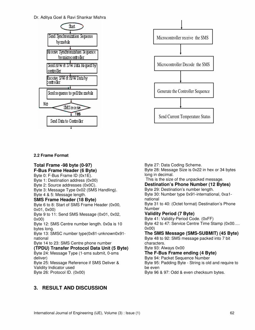
Dr. Aditya Goel & Ravi Shankar Mishra
International Journal of Engineering (IJE), Volume (3) : Issue (1) 62
Microcontroller receive the SMS
Microcontroller Decode the SMS
Generate the Controller Sequence
Send Current Temperature Status
2.2 Frame Format
Total Frame -98 byte (0-97) F-Bus Frame Header (6 Byte) Byte 0: F-Bus Frame ID (0x1E). Byte 1: Destination address (0x00) Byte 2: Source addresses (0x0C). Byte 3: Message Type 0x02 (SMS Handling). Byte 4 & 5: Message length.
SMS Frame Header (18 Byte) Byte 6 to 8: Start of SMS Frame Header (0x00, 0x01, 0x00) Byte 9 to 11: Send SMS Message (0x01, 0x02, 0x00) Byte 12: SMS Centre number length. 0x0a is 10 bytes long. Byte 13: SMSC number type(0x81-unknown0x91-national Byte 14 to 23: SMS Centre phone number
(TPDU) Transfer Protocol Data Unit (5 Byte) Byte 24: Message Type (1-sms submit, 0-sms deliver) Byte 25: Message Reference if SMS Deliver & Validity Indicator used Byte 26: Protocol ID. (0x00)
Byte 27: Data Coding Scheme. Byte 28: Message Size is 0x22 in hex or 34 bytes long in decimal. This is the size of the unpacked message. Destination’s Phone Number (12 Bytes) Byte 29: Destination’s number length. Byte 30: Number type 0x91-international, 0xa1-national Byte 31 to 40: (Octet format) Destination’s Phone Number
Validity Period (7 Byte) Byte 41: Validity-Period Code. (0xFF) Byte 42 to 47: Service Centre Time Stamp (0x00…. 0x00)
The SMS Message (SMS-SUBMIT) (45 Byte) Byte 48 to 92: SMS message packed into 7 bit characters. Byte 93: Always 0x00
The F-Bus Frame ending (4 Byte) Byte 94: Packet Sequence Number Byte 95: Padding Byte - String is old and require to be even Byte 96 & 97: Odd & even checksum bytes.
3. RESULT AND DISCUSSION

Dr. Aditya Goel & Ravi Shankar Mishra
International Journal of Engineering (IJE), Volume (3) : Issue (1) 63
TABLE 1: Synchronization Pattern for temperature TABLE 2: Temperatures Status on PC
TABLE 3: Synchronization Pattern Energy meter TABLE 4: Energy meter Status on PC
FIGURE 5: Temperature Status on Mobile FIGURE 6: Energy meter reading on Mobile
The F-Bus cable is High-speed full duplex bus. It uses one pin for transmitting data and one pin for receiving data plus one ground pin. The F-Bus is bidirectional serial type bus running at 115,200bps,8 data bits, no parity and one stop bits. For synchronizing UART in the phone with micro controller, string of 0x55 or ‘U’ was send 128 times. The NOKIA Protocol has a series of commands that allow the user to make calls, send and get SMS. The NOKIA frame consists information about source address, destination address and message length. In NOKIA Frame format the SMS message packed into 7 bit characters. The last byte in the data segment is sequence number. The last 3 bits of these bytes increments from 0 to 7 for each frame. This part is used as acknowledgement frame.4 The synchronizing frame sent to synchronize the mobile and controller. After sending synchronizing frame that is 128 times “U” or 0x55, PC shows the seven sequence number from S=40 to S= 47 on which message should receive. After receiving the request message, the 58 byte frame format is formed in that format last 3rd and 4th byte is used as CRC check byte .The CE and CO is the even and odd CRC check bits which is decided by length of the message. TABLE 1 and TABLE 3 shows the results of synchronization pattern display on PC with the F-bus cable of temperature monitoring and meter reading. TABLE 2 and TABLE 4 show the temperature and energy status on PC and the FIGURE 5 and FIGURE 6 shows the current temperature and energy status on mobile phone.4
Synchronizing...S==40 CE=21 CO=f4 S==41 CE=20 CO=f4 S==42 CE=23 CO=f4 S==43 CE=22 CO=f4 S==44 CE=25 CO=f4 S==45 CE=24 CO=f4 S==46 CE=27 CO=f4 S==47 CE=26 CO=f4
Printing... Current temperature status is 20 deg S==46 CE=13 CO=44 S==47 CE=52 CO=d5 Printing... Current temperature status is 30 deg
Synchronizing...S==40 CE=21 CO=f4 S==41 CE=20 CO=f4 S==42 CE=23 CO=f4 S==43 CE=22 CO=f4 S==44 CE=25 CO=f4 S==45 CE=24 CO=f4 S==46 CE=27 CO=f4 S==47 CE=26 CO=f4
Printing... Current meter reading is 223 KWH S==42 CE=13 CO=42 S==43 CE=52 CO=e5 Printing... Current meter reading is 224 KWH

Dr. Aditya Goel & Ravi Shankar Mishra
International Journal of Engineering (IJE), Volume (3) : Issue (1) 64
4. CONCLUSION AND FUTURE SCOPE
Our objective is to work on the “Remote site Safety & security Application by using Controller” to achieve to produce an input data file for each of the Data Logger, build a Controller Area network ,Collect & manage data in the Control Area Network(CAN) and Send SMS to a monitoring centered . GSM communication performed almost flawlessly data transfer from sensor at remote area was executed Without incidents. Since all communication between data logger and user are wireless based, this translates into lowest cost compared to all others system. In this project all the database is stored in a central database in the data logger; user has global access to consolidate data from many system or locations. Wireless based solutions have universally accepted, familiar and user friendly system. Real-time logging would allow warnings to be flagged to the relevant personnel (e.g. an SMS warning message to the supervisors) and allow corrective action to be taken before the quality and value of the catch is degraded. With the proposed setup in Figure 3 temperature was successfully monitored remote location and it was measured to be around 30
oC. Similarly energy meter reading from remote location was also successfully
implemented using demonstrated hardware setup of wireless SCADA system. The recorded energy meter reading as demonstrated in Figure2 is 223 KWH. Hence the wireless SCADA system is powerful setup for monitoring and controlling the various applications from remotely placed location. It can be further extended for various area of application like health monitoring system, Home security system, Vehicle Security system etc.
5. REFERENCES
1. Sungmo Jung, Jae-gu Song, Seoksoo Kim, “Design on SCADA Test-bed and Security Device,” International Journal of Multimedia and Ubiquitous Engineering, Vol. 3, No. 4, October, 2008
2. Sandip C.Patel, Pritimoy Sanyal ” Securing SCADA System” Information Management & Computer
Security Journal Volume: 16 Issue: 4 Page: 398 – 414 Year: 2008
3. Gumbo, S, Muyingi, H, “Development of a web based interface for remote monitoring of a Long-distance power transmission overhead line”, SATNAC 2007, Sugar Beach Resort, Mauritius, ISBN 978 0 620 39351 5
4. http://www.embedtronics.com. online details of frame format of NOKIA 5. Surve, V, 2006, “A wireless Communication Device for Short Messages”, Masters Thesis,
Available: www.certec.lth.se/doc/awireless.pdf.
6. Das, AN, Lewis, FL, Popa, DO, 2006, “Data-logging and Supervisory Control in Wireless Sensor Networks,” Proceeding of the Seventh ACIS International Conference on Software Engineering, Artificial Intelligence, networking, and Parallel/Distributed Computing (SNPD’06), Volume 00, ISBN:0-7695-2611-X, pp 330- 338 7. Hildick-Smith, Andrew, “Security for Critical Infrastructure SCADA Systems,” (SANS Reading Room, GSEC Practical Assignment, Version 1.4c, Option 1, February 2005),
http://www.sans.org/reading_room/whitepapers/warfare/1644.php
8. Carlson, Rolf E. and Jeffrey E. Dagle, Shabbir A. Shamsuddin, Robert P. Evans, “A Summary of Control System Security Standards Activities in the Energy Sector,” Department of Energy Office of Electricity Delivery and Energy Reliability,66 National SCADA Test Bed, October 2005, http://www.sandia.gov/scada/documents/CISSWG_Report_1_Final.pdf 9. Technical Information Bulletin 04-1, Supervisory Control and Data Acquisition (SCADA) Systems, NCS TIB 04-1, Oct. 2004
10. I. F. Akyildiz, W. Su, Y. Sankarasubramaniam, and E. Cayirci, "A Survey on Sensor Networks," IEEE

Dr. Aditya Goel & Ravi Shankar Mishra
International Journal of Engineering (IJE), Volume (3) : Issue (1) 65
Communications Magazine, Vol. 40, No. 8, pp. 102-114, August 2002; receives the IEEE Communications Society 2003 Best Tutorial Paper Award, April 2003.
11. Bement, Arden “Keynote Address at the NSF Workshop on Critical Infrastructure Protection for
SCADA & IT,” October 20, 2003, http://www.nist.gov/speeches/bement_102003.htm .
12. McClanahan, R.H.,” The Benefits of Networked SCADA Systems Utilizing IP Enabled Networks", Proc. Of IEEE Rural Electric Power Conference 5-7 May 2002 Pages: C5 - C5_7
13. Dagle, J.E.; Widergren, S.E.; Johnson, J.M.” Enhancing the security of supervisory control and data acquisition (SCADA) systems: the lifeblood of modern energy infrastructures” Power Engineering Society Winter Meeting, 2002. IEEE Volume 1, Issue , 2002 Page(s): 635 vol.1
14. J.E. Dagle (SM), S.E. Widergren (SM), and J.M. Johnson (M)” Enhancing the Security of Supervisory Control and Data Acquisition (SCADA) Systems: The Lifeblood of Modern Energy Infrastructures” Power Engineering Society Winter Meeting, 2002. IEEE Volume 1, Issue, 2002 Page(s): 635 vol.1
15. Stephen Beasley, Mr Choon Ng Dr Dario Toncich and Dr Andrew Dennison “Remote Diagnostics for Data Acquisition Systems” white paper by Industrial Research Institute Swinburne Available online at
www.swinburne.edu.au/feis/iris/pdf/profiles/StephenBeasley.pdf 16. Taylor, K; “Mobile Monitoring and Control Infrastructure”, CSIRO Available online at http://mobile.act.cmis.csiro.au
Ming-Chang Huang, Seyed Hossein Hosseini, K.Vairavan & Hui Lan
International Journal of Engineering (IJE), Volume (3) : Issue (1) 65
Fuzzy Congestion Control and Policing in ATM Networks
Ming-Chang Huang
[email protected] Department of Math & Information Systems University of Phoenix at Charlotte Charlotte, NC 28270
Seyed Hossein Hosseini [email protected]. Department of Electrical Engineering and Computer Science University of Wisconsin-Milwaukee, P.O. Box 784 Milwaukee, Wisconsin 53201
K. Vairavan [email protected]. Department of Electrical Engineering and Computer Science University of Wisconsin-Milwaukee, P.O. Box 784 Milwaukee, Wisconsin 53201
Hui Lan Department of Electrical Engineering and Computer Science University of Wisconsin-Milwaukee, P.O. Box 784 Milwaukee, Wisconsin 53201
ABSTRACT
In this paper, usage parameter control (UPC) is presented to ensure that each source conforms to its negotiated parameters in ATM networks. To meet the requirements for the policing function, a fuzzy logic-based system is proposed to deal with the congestion control and policing problem in ATM networks. There are four types of different mechanisms, Jump Window (JW), Exponentially Weighted Moving Average (EWMA), Leaky Bucket (LB) and modified Fuzzy Leaky Bucket (FLB) techniques to be identified, analyzed and simulated by the traffic parameters. The Fuzzy Leaky Bucket (FLB) modifies the token rate in accordance with the peak rate, mean rate and the burst time, which characterize the source behavior. Simulation results show that FLB system is transparent to the sources with the parameter values which are negotiated at the call setup and effective in detecting source violation with low response time. The performance of FLB is significantly better than other mechanisms, in terms of both dynamic behaviors of responsiveness and selectivity. Keywords: ATM, Fuzzy Logic, Leaky Bucket, Jump Window, Exponentially Weighted Moving Average
1. INTRODUCTION
Based on today’s telecommunication system and potential requirements, it is easy to predict that the future is the time of network. To support the future’s applications, telecommunication should have the following characteristics: broadband, multimedia, and economical implementation for the diversities of services. Broadband integrated services and digital networks (B-ISDN) provide what are in need at present and in the future. Asynchronous Transfer Mode (ATM) is a targeted
Ming-Chang Huang, Seyed Hossein Hosseini, K.Vairavan & Hui Lan
International Journal of Engineering (IJE), Volume (3) : Issue (1) 66
technology for meeting these requirements [3, 4, 15, 14, 25]. In ATM network, the information is transmitted by using short fixed-length cells (cell switch) - which reduces the delay variance - makes it suitable for transmission in new high-speed integrated service networks, such as voice, video and data. Meanwhile, ATM can ensure efficient operation to process the flexibility which is invited to support services with different rates, qualities of service (QoS) and characteristics. The asynchronous statistical multiplexing may also improve the utilization of the bandwidth for the traffic flows. In ATM network, a proper traffic control management is required to guarantee a certain QoS in terms of delay and cell-loss probability. The fluctuation of random traffic would cause a serious congestion problem for the network if the network exists (runs) without proper policing mechanism. An effective control mechanism is imperative to maintain a balance between the QoS and network utilization both at the time of call setup and during the progress of the calls across the ATM network. The control mechanism that allocates resources and judges rejection or acceptance of the connection is usually called Connection Admission Control (CAC) [3,4], and the control mechanism that monitors and smoothes the rate of the traffic during the call setup phase is normally called policing or Usage Parameter Control (UPC) [3, 4]. Policing is used to ensure the sources to stay between their declared rate limits (traffic contract); thus, it will not affect the performance of the network. In the case that a source disobeys its contract, the network provider would block the source or selectively drop packets by tagging packets (set CLP=1), which will be selectively dropped by priority bit if necessary when congestion occurs in the network. The traditional ATM networks use Leaky Bucket method as one of its policing mechanism. In this mechanism, it uses fixed threshold buffer size for store the tokens for traffic control purpose. In order to improve the performance of ATM networks, we use a virtual leaky bucket with fuzzy logic control to control the depletion rate in the bucket. We compare this Fuzzy Leaky Bucket mechanism with other policing mechanisms - Jump Window (JW), Exponentially Weighted Moving Average (EWMA), and traditional Leaky Bucket (LB). We have the simulations for comparing the results of these four mechanisms. This paper is organized as follows. Section 2 introduces the traffic management in an ATM network. Section 3 addresses conventional policing mechanism in ATM network and Section 4 presents the Fuzzy Leaky Bucket Algorithm (FLB). Section 5 shows the comparison, simulation results and analysis. Section 6 is our conclusion.
2. TRAFFIC MANAGEMENT IN AN ATM NETWORK
Although the circuit switch system has been developed for about 100 years, e.g. the public telephone system, and even the packet switch has existed for over 50 years, however, no good solution has been found to the problem of the ATM network traffic and congestion control. A more formidable task is the management of the digital applications: image, voice, video, and data applications in a coherent and integrated fashion. The factors that contribute to the complexity of traffic and congestion control in the ATM networks are as follows: 1. Different traffic sources have different speed magnitudes. The speed from one terminal to
another is only a few kbps/s, but for HDTV, it is required to take a few Mbps/s bandwidth. Some application bit cell rate is changed by time characteristic.
2. Single traffic source may generate different traffic with different characteristic, for example, voice, data, or even picture and video.
3. Except the performance measure factors, such as call block and package switch loss ratio used in the current network, ATM is also requested to process CDV, MDV and image shift.
4. Different services have different QoS magnitude requirements. With the assumption of putting together VBR and CBR traffic, statistic multiplexing in multi-links in the same transmit

Ming-Chang Huang, Seyed Hossein Hosseini, K.Vairavan & Hui Lan
International Journal of Engineering (IJE), Volume (3) : Issue (1) 67
medium is complicated and it is hard to predict what the upcoming performance will be for these two network. Especially, the QoS of real time service can be easily harmed.
5. Different traffic characteristic should be studied and analyzed. As long as the transfer speed increases, call-waiting time vs. cell transmit time will increase simultaneously, which requires a higher level. Since high-speed data link has broad transfer delay, there will be huge cells moving at any point in the network. Furthermore compared with the submitting time, when the congestion occurs, the bigger the transfer delay is, the longer it will take for the network to detect what the congestion components are. High transfer speed also limits the processing time among the internal node for processing the congestion.
Due to the high transfer speed, the congestion method should be an easy implementation for the hardware. For each connection, the QoS parameters should be supported and satisfied from the beginning of call setup to the end, in spite of other connections’ traffic characteristics and sources behaviors in the network. At most time the traffic source (customer) may not describe its traffic characteristics accurately enough. So, the good control technique should not only use these sample source traffic characteristics but also be steady enough to reduce the influence from the inaccurate traffic characteristics. In this environment, it is not an appropriate idea to use manual ways to limit user traffic characteristic. For example, the cell speed may be reduced before the call set-up and transfer to decrease the connection peak cell rate. Unfortunately, it is unacceptable for the time-delay sensitive application, though it may smooth the traffic in the network and make it easier to manage. An improper congestion control design may decrease the utilization of network. ATM network, as it is required, is designed to support not only the current but also the future applications, such as high bandwidth multi-media applications. A properly constructed ATM network should manage traffic fairly, provide effective allocations of the network capacity for different sorts of applications, and perform cost effective operations at the relative service level (QoS) stipulated by the network users. Meanwhile the network should support the different delay requirements of the applications, an important support function known as cell delay variation (CDV) management. ATM network is required to be able to adapt to unforeseen traffic patterns, for example, unusual bursts of traffic from the various end-user devices or applications. The network also should have the ability to shed traffic in certain conditions to keep it from or react to congestion. For protection, network must be able to enforce an allowable peak cell rate for each VPI/VCI connection. That is to say, it may be discarded on the occasion when a user's traffic load submitted to the network goes beyond the maximum peak rate. In addition to these responsibilities, the network should be able to monitor traffic, and all VPI/VCI connections, and verify their behaviors. The network must also detect problems, and emit alarms when they happen. An effective ATM network is designed with an understanding for both the user and network to assume responsibility for QoS operations between them. The user should agree with the service contract that ATM network stipulates the rules, such as the amount of traffic that can be submitted in a measured time period. On the other hand, the network assumes the responsibility of supporting the user QoS requirements. The fuzzy logic control method has been used in different ways. Lekcharoen et. Al, [11, 12] use the fuzzy logic control in QoS in wireless networks and in QoS sensitive backoff schemes. They use FLC in the buffer size and the fixed leak rate. It also uses it in Triggered Jumping Window(TJW). Lekcharoen, S. and Jittawiriyanukoon also discuss the policing mechanisms in deadlock of avoidance backoff schemes. Koutsakis, P and Paterakis, M. [30] use policing mechanisms in ATM networks the video-conference traffic in wireless ATM. Fuzzy logic control has also been used in the management of ATM networks [1, 2, 21]. In this paper, we add a virtual leaky bucket based on fuzzy logic control in controlling the buffer size and the leaky rate of tokens.

Ming-Chang Huang, Seyed Hossein Hosseini, K.Vairavan & Hui Lan
International Journal of Engineering (IJE), Volume (3) : Issue (1) 68
3. CONVENTIONAL POLICING MECHANISM IN ATM NETWORK
Traffic control is a function protecting the network from congestion. The main goal of the traffic control in any networks is to achieve the required network performance objectives. In ATM network, traffic policing is located at the access point to the User Network Interface (UNI). What traffic policing does is to check the validity of VPI and VCI values and monitor the cells arriving at the network and determines whether it violates any parameters. In ATM network this is called the Usage parameter Control (UPC). It detects any nonconforming sources and the necessary actions it takes are as follows: 1. To dropping violating cell 2. To delay violating cells in queue 3. To mark violating cells and treat them accordingly 4. To control traffic by informing the source to take action when violation occurs. Two most popular methods exist in UPC to control the peak rate, mean rate and different load states. They are Leaky Bucket method and Window Method.
3.1 Leaky Bucket Algorithm (LB)
The most famous, popular and simplest policing method is the Leaky Bucket (LB) mechanism, which was first proposed by Turner (1986) [3, 4, 15, 14, 24, 29, 25, 28, 8]. In fact, it is similar to a single-server queuing system with a constant service time. The host is allowed to put one packet per clock tick onto the network. This mechanism turns an uneven flow of packets of user processes into the host and outputs an even flow of packets onto the network. It smoothes out bursts and greatly reduces the chances of congestion. But for many applications, it is better to speed up the output when large bursts arrive. Therefore a more flexible algorithm is needed and the token bucket algorithm is one of them. In this algorithm,
the leaky bucket holds tokens generated by a clock at the rate of one token every ∆T seconds. The packets must hold token to get into the network. The token bucket algorithm throws away tokens when bucket is filled up. A figure for Token Bucket algorithm is illustrated below.
The basic idea about token leaky bucket is that before a cell enters a network, the cell must obtain a token from a token pool. Upon consuming a token, the cell will immediately leave the leaky bucket. Tokens are constantly generated and placed in the token pool. There is a maximum number of tokens waiting in the pool. The size of the token pool will impose an upper bound on the burst length and determine the number of cells that can be transmitted to control the burst. As long as the queue is not empty, the cells are transmitted with the constant rate of the service rate. So the LB algorithm can receive burst traffic and control the output rate. If excess traffic
N
λ
FROM THE
SOURCE DROPPING
SWITCH TO THE
NETWORK
CONTROL
SIGNAL

Ming-Chang Huang, Seyed Hossein Hosseini, K.Vairavan & Hui Lan
International Journal of Engineering (IJE), Volume (3) : Issue (1) 69
makes the buffer overflow, the algorithm can choose to discard the cells or tag them with CLP = 1 and transmit them into network. In this token bucket algorithm, choosing appropriate values of service rate and buffer size can control PCR or SCR. From another viewpoint, the LB mechanism consists of a counter, which is increased by 1 each time a cell is generated by the source and decreased in a fixed interval as long as the counter value is positive. At that time, cell arrival rate exceeds the decreased (leak/drain) rate; the counter value starts to increase. It is assumed that the source expects admissible parameter range on the occasion the counter reaches a predefined limit. The suitable actions (e.g. discard or tag cells) are taken on all subsequently generated cells until the counter has fallen below its limit again. This mechanism is quite easy to be implemented.
Two important parameters for LB are the threshold N and depletion (leak/drain) rate λd. In
principle, in enforcing the mean cell rate to equal the negotiated mean cell rate, that is, λd = λn, the parameter N plays a very important role. Threshold N values can control the burstiness degree of LB. When N values are high, the allowance of burstiness degree and reaction time of the mechanism grows excessively; the cell loss ratio gets lower. Vice versa, the cell loss ratio turns higher. Since a cell has burstiness characteristic, in order to achieve greater flexibility in buffer size and reduce the probability of false alarms, it is necessary to introduce an over
dimension bursty detective scope factor C (C≥1) between the negotiated cell rate λn, and really
policed cell rate λp. It follows that λd = λp = Cλn. On the other hand, it may reduce the capacity to detect violation over a long term. Especially in an extreme case of a deterministic source, the traffic generates cells may even exceed the negotiated cell rate up to a scope factor C without any cell being detected. In spite of its drawback, the LB mechanism is still popular and in wide use due to its simple implementation.
3.2 Jump Window Algorithm (JW)
Other control methods are the window-based policing mechanism that regulates the traffic flow submitted to the network. In simple terms, window methods can be described as a method limiting the number of cells in a time window. Basically, the Jumping Window scheme imposes an upper bound on the number of cells accepted from a source during a fixed time interval referred to as the window. The new interval starts immediately after the end of the processing interval (jumping window) and the associated counter is restarted again with an initial value of zero. Once the upper bound is reached, all consecutively arriving cells are dropped and are not allowed to enter the network. These excessive cells then can be marked as low-loss priority using cell loss priority (CLP) bit [14, 7, 19]. Therefore, the length of the window is fundamental for the performance of mechanism. The time interval during specific cell influences the counter value varies from zero to window width N. Since JW does not have a queue mechanism, it is normal for JW to ask for a big window size; consequently JW does not have a good detective ability.
3.3 Exponentially Weighted Moving Average Algorithm (EWMA)
Another well known window-based mechanism is the Exponentially Weighted Moving Average [14, 7, 19]. This scheme is similar to jumping window in which the window size is permanent and a new window is triggered immediately after the proceeding one ends. The difference between this scheme and the jumping window is that the number of cells accepted during one window varies from another. The EWMA mechanism uses fixed consecutive-time windows like the JW mechanism. However, unlike the JW, the limit of the max number (window size) is unfixed. For EWMA, the big difference is that the maximum number of accepted cells in the ith window (Ni) is a function that allows the mean number of cells per interval (windows), N, to be dynamically updated. An exponentially weighted sum of the number of accepted cells in preceding intervals (Xi) are significantly relate to the past amount (burstiness of cell rate), i.e., the number of accepted cells in the previous intervals. To calculate the max Ni in the ith window, the formula can use as below:

Ming-Chang Huang, Seyed Hossein Hosseini, K.Vairavan & Hui Lan
International Journal of Engineering (IJE), Volume (3) : Issue (1) 70
γ
γ
−
−= −
1
1ii
SNN
0γ≤
< 1 with
Si-1 = (1-γ) X i-1 + γ Si-2 which can also be expressed as
( )( )γ
γγγγ
−
−++−−=
+−−
1
.......1 0
1
1
1
1 SXXNN
ii
ii
where S0 is the initial value of the EWMA measurement; it is a constant given at random, which is usually set at S0 = 0. Ni is the max number of cell that can be received in ith window; N is the mean number of cell that can be received in each window; Xi is the number of cell already received in ith window.
The constant weighting factor γ controls the flexibility more or less of the traffic burst. γ is a
coefficient given randomly between the range of [0,1]. If γ = 0, Ni is constant and the algorithm is the same as the traditional JW mechanism. EWMA performance depends greatly on the value
chosen for γ: for respectful sources, a high value is required; on the other hand, for violating sources it has to be low. The limit of this mechanism is its static nature and the prior choice of
the value of γ. The implementation complexity of the mechanism EWMA is more complex than that of the
previous mechanisms. The formula above may lead to a conclusion that, for different γ; the changing degree of Ni is different. Ni is related to the number of the real arriving cells in the previous window, and the degree of influence on Ni is different in every window as well. The closer it is to the current window, the more influence on Ni will be present, and vice versa. EWMA mechanism is derived from JW. In EWMA, the monitor window can be changed based on the cell bursty condition. However, cell bursty situation can only be reflected from the formula and cell traffic can only be shown in a certain degree.
4. FUZZY LEAKY BUCKET ALGORITHM (FLB)
ATM is selected as the final transfer model of B-ISDN for its advantages: higher transfer speed, higher degree of flexibility and better network resource utilization. However, these advantages also make ATM more difficult in traffic and congestion control compared with the traditional circuit switch and packet switch. ATM network must deal with the integrated traffic sources and unpredictable “bursty” traffic. To improve the transfer speed, the preventive congestion control of the ATM network only affects the edge of network to control the possible congestion. According to the discussion above, there are two relevant concepts: CAC and UPC. Based on the ITU-T I.371 suggestion, there exist two main parameters to evaluate the performance of congestion control: response time and transparence. Response time is the degree of quick reaction of the UPC policing mechanism to detect the violated cells. Transparence shows the discrimination ability of selectivity between goodness and badness, normality and abnormality. In an ideal situation, non-violated cell is capable to get through the network safely, and without any policing mechanism. Violated cells should be detected and eliminated completely. However, there is no ideal policing mechanisms. The good policing mechanism is close to an ideal one and it is inexpensive and easy to achieve. However, none of the above conventional mechanisms is able to meet with all the requirements of an ideal policing because practically mathematical models are not easily defined. For unconventional mechanisms, fuzzy logic is a powerful, straightforward, problem-solving technique with wide-spread applicability, especially in the areas of control and decision-making.

Ming-Chang Huang, Seyed Hossein Hosseini, K.Vairavan & Hui Lan
International Journal of Engineering (IJE), Volume (3) : Issue (1) 71
Fuzzy logic derives much of its power from its ability to draw conclusions and generates responses based on vague, ambiguous, incomplete or imprecise information. Upon this respect, fuzzy systems have a reasoning ability similar to that of humans. In fact, the behavior of a fuzzy system is represented in a simple and natural way. In this paper, a fuzzy logic-based system, fuzzy leaky bucket (FLB), is presented to deal with the congestion control problem in the ATM networks. FLB is based on a fuzzy logic implementation of virtual leaky bucket (VLB) and also on the fuzzy control theory [17, 20, 10] with rules such as: Rule: If the cell number in leaky bucket buffer is high and virtual leaky bucket counter number is medium then reduce the token rate and drop violating cells Where high and medium are linguistic labels of fuzzy sets in a given universe of discourse. In the synthesis of fuzzy leaky bucket controller, the control goal and strategy are stated linguistically but mapped into fuzzy sets and manipulated mathematically. The objective is to control the cell rate by fuzzy expert knowledge in the ATM congestion control, rather than depend on the mathematical formulation of classical control theory. This paper is organized as follows: ATM traffic control issues, source traffic models, and introduction of the fuzzy logic control (FLB) mechanism. The simulation results and conclusion are provided at the end.
4.1 ATM Traffic Fuzzy Control Issues
The wide range of service characteristics, bit rates, and burstiness factors in the broadband networks combined with the need for flexible control procedures makes the traditional control methods very difficult to apply. It is impossible to analyze all the involved different traffic cases and traffic situations arising in an ATM network. Moreover, it is also difficult to update if there are new services introduced. Non-traditional control methods, on the other hand, contain the ideas and techniques of neural networks and fuzzy logic may use adaptive learning and are flexible enough to support a variety of criteria and wide range of parameters. Fuzzy logic has rapidly been developed as one of the most successful technologies today in the field of sophisticated control systems. It makes the control much smoother based on the linguistic variables. The reason is simple. Fuzzy logic processes some applications perfectly. For example, it may resemble or simulate human decision by developing an ability to generate precise solutions for certain or approximate information. It fills an important gap in engineering design methods that are left vacant by purely mathematical approaches (e.g. linear control design) and purely logic-based approaches (e.g. expert systems) in system design [17, 26, 20].
4.2 Fuzzy Control for ATM Policing
In order to give an example of how fuzzy inference rules can be defined in a typical ATM control, this section presents the fuzzy control for UPC purposes. The fuzzy policer is a mechanism, a threshold token rate R updated dynamically by the inference rules based on fuzzy logic. The goal of this fuzzy policer is to make the source respect to the negotiated contract, which is the mean cell rate over the duration of the connection. According to the expected behavior of an ideal policing mechanism, short-term fluctuations should be allowed as long as the long-term negotiated parameter is respected, and it should also be able to recognize a violation immediately. More specifically, the control mechanism grants credit to a source, which has respected to the parameter negotiated in the past, by increasing its control threshold token rate R as long as it maintains with non-violating behavior. Vice versa, if the source behavior is violating or risky, the mechanism reduces the credit by decreasing the threshold token rate value. In the fuzzy control system, the parameters describing the source behavior and the policing control variables are made up of linguistic variables and fuzzy sets. Then action of control is

Ming-Chang Huang, Seyed Hossein Hosseini, K.Vairavan & Hui Lan
International Journal of Engineering (IJE), Volume (3) : Issue (1) 72
expressed by a set of fuzzy conditional rules. The rules reflect the cognitive processes and knowledge that an expert in the field would apply.
4.3 Fuzzy Logic Control FLB Mechanism
The Leaky Bucket (LB) mechanism is considered an effective method of UPC in ATM networks, but the conventional LB algorithm is difficult to be implemented on some conflicting requirements such as cell loss probability and mean time delay. It is difficult to monitor the mean rate and the peak rate at the same time. It is known that token rate should be around in the neighborhood of the peak rate and the buffer length has to be low for the mechanism to react effectively to the peak cell rate variations. In other words, in order to control the mean rate, the token rate has to be around mean rate and the buffer length is high. An ideal control mechanism is fast to act on cells violating the contract and limit the influence of an "ill-behaving" source on the quality of service provided for all connections sharing the network resources. More specifically, it should be transparent to connections with the traffic contract. Fuzzy logic based system has demonstrated the abilities to make intelligent decisions, perform calculations on imprecise quantities and model linguistic rules where precise mathematical models are impractical or unavailable. The inherited capacity formalize approximate reasoning processes offered by fuzzy logic is exploited to build a dynamic control mechanism, which is expected to smooth the rate of the traffic and improve the utilization efficiency of bandwidth [6, 17, 26, 20]. It should be pointed out that the token rate R and leaky bucket buffer length are crucial to cell loss rate and mean time delay. It is difficult to change the leaky bucket buffer length, but it is a proper choice to modify the token rate R. When the source has gained credit, R would be high to improve the utilization efficiency of bandwidth and decrease the time delay. Vice versa, if the source begins to violate, the R would be low to detect the long statistical fluctuation quickly. The FLB controller belongs to a general fuzzy control system in which control variables are transformed into fuzzy sets (Fuzzification) manipulated by a collection of IF-THEN fuzzy rules, and assembled in what is known as the fuzzy inference engine. These rules are derived from the knowledge of experts with substantial experience in the leaky bucket mechanism and ATM traffics. The FLB is a rule-based expert system. However, unlike expert systems, the FLB uses the membership function to generate approximate control actions to deal with different scenarios. This capability allows the FLB controller to compensate for ambiguities in the control rules; and it is common in the bursty environment that characterizes the ATM traffic cells. The modified LB technique has been combined in this paper to identify the traffic parameters. The modified FLB in our implementation is dimensioned for mean cell rate. The mean cell rate determines the long-term average transmission rate. Traffic falling under this rate will always be conformed, and the amount of the cells in the LB shows the burst time. The Fuzzy Leaky Bucket (FLB) modifies the token rate according to the mean rate and the burst time, which characterize the source behavior. The model of FLB is shown as Figure 1. This fuzzy leaky Bucket system is on the basis of fuzzy logic control. The virtual leaky bucket is designed to monitor the mean cell rate as cells pass through the ATM switch node and actually enter the network. Virtual leaky bucket leak speed Rv is equal to the negotiated mean cell rate Rneg. In another viewpoint, virtual leaky bucket can be considered as a cell number counter. Virtual leaky bucket is assigned an initial number Ni; the number that is related to the traffic flow characteristic. After traffic passes through the ATM switch node and gets into the network, each cell generates a virtual cell to get into the virtual leaky bucket. When a virtual cell comes out in the virtual leaky bucket, the virtual leaky bucket will keep leaking virtual cell at the rate Rv. Consequently, when the number of virtual cells in the virtual leaky bucket is greater than the initial number Ni, means the real mean cell rate getting into the network is higher. When the number of counter goes up, the deviation of cell gets bigger simultaneously, that means the mean cell rate is too high. On the other hand, when the number of virtual cells in the virtual leaky bucket is less than the initial

Ming-Chang Huang, Seyed Hossein Hosseini, K.Vairavan & Hui Lan
International Journal of Engineering (IJE), Volume (3) : Issue (1) 73
number Ni that means the mean cell rate getting into the network is low. The degree or deviation of lower value varies according to the number of counter. As shown in Figure 1, FLB consists of two fuzzy logic inputs: virtual leaky bucket counter number N and cell number in the leaky bucket buffer X. Virtual leaky bucket counter number N shows the cell burstiness. Meanwhile it also indicates its current behavior. Cell number in the leaky bucket buffer X is not fixed; it is based on the mean cell rate, current burst and up to negotiate peak cell rate. It may be greatly changed in a short period of time and give an indication of the long-term trend of the source. So, one type of corresponding relationship exists between the virtual leaky bucket counter number N and the cell number X in the leaky bucket buffer. However, this corresponding relation is hard to be described accurately in a conventional math model. Therefore, the traditional control method would not work well and efficiently. However, in this area fuzzy logic control does not require an accurate math model. The sample control rules are applied for controlling the system.
The work principle of the FLB is: FLB chooses the cell number X in the leaky bucket buffer and virtual cell number N in the virtual leaky bucket (cell counter) as the crisp input parameters. After the three-step procedures: fuzzification, rules evaluation (make decision) and defuzzification, FLB
gets the crisp output value K, K (0,1), then adjusts the token rate R=K• h (h =PCR). After testing the membership functions chosen for the fuzzy sets, the above parameters are fuzzified by linguistic values shown in Figure 2~4. The input and output variables are divided into five fuzzy subsets: Very Low (VL), Low (L), Medium (M), High (H), Very High (VH).
Sources Network
Fuzzification
Fuzzy Reference
Token Rate Control
Defuzzification
Leaky Bucket
Token Buffer
CAC
X R
K
Fuzzy Logic Leaky Bucket (FLB) Controller
FIGURE 1: The Model of Fuzzy Control System (FLB)
N
Virtual Leaky
Bucket
Rv

Ming-Chang Huang, Seyed Hossein Hosseini, K.Vairavan & Hui Lan
International Journal of Engineering (IJE), Volume (3) : Issue (1) 74
Fuzzy conditional rules for the policer are given in Table 1. The case will be discussed in which the source is fully respectful. When cell in leaky bucket buffer X is Low, thus, if N, the number of cells in virtual leaky bucket, is Low or Medium, that is, the source continues a non-violating behavior; its credit is increased and token rate K will be increased. If N is High, a sign of a possible violation on the part of source, K will be reduced to Medium correspond to the X is L. The other rules can be interpreted analogously.
X N
VL L M H VH
VL VH VH VH H L
L VH VH H M L
M VH H M L VL
H H M L VL VL
VH M L VL VL VL
Table 1: Fuzzy Rules
The Max-Min (Mamdani) inference and Centroid (center of gravity) defuzzification are used in this paper. The output value is the weight average of the individual outputs of the rules. The output can be calculated as follows:
where )( iZµ
is the fitness value of the ith fuzzy rule, iZ is the center value of the output
membership functions of the ith item of the output linguistic variable, *Z means the
defuzzification output K in this paper. The Flb_3D_Surface curve of output K is shown in Figure 5. The Flb_3D_Surface curve of output K is a control surface. With two inputs N and X and one output Z, the input-output mapping is a surface. It’s a mesh plot of an example of the relationship between N and X on the input side, and FLB controller output Z on the output side. The plot is based upon 25 rules. The 3D-output curve also shows the relationship between the output and
FIGURE 3: Membership function for the N input variable
µ
VL L
M
H
VH
0 0.8 N 0.9 N N 1.1 N 1.2 N
1.0
N
Figure 4: Membership function for K output variable
VL L M H VH
µ
1.0
0 0.25 0.5 0.75 1.0
K
VL L M H VH
0 0.25 M 0.5 M 0.75 M
1.0
X
FIGURE 2: Membership function for the X input variable
M: the length of leaky bucket buffer.
N: the number of virtual cells in VLB.
M
µ
( )( )∑
∑=
i
ii
Z
ZZZ
µ
µ*
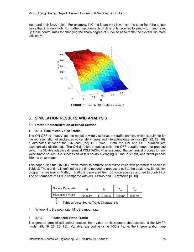
Ming-Chang Huang, Seyed Hossein Hosseini, K.Vairavan & Hui Lan
International Journal of Engineering (IJE), Volume (3) : Issue (1) 75
input and their fuzzy rules. For example, if X and N are very low, it can be seen from the output curve that Z is very high. For further improvements, FLB is only required to simply turn and reset up those control rules for changing the sharp degree of curve so as to make the system run more efficiently.
5. SIMULATION RESULTS AND ANALYSIS
5.1 Traffic Characterization of Broad Service
1 5.1.1 Packetized Voice Traffic
The ON-OFF or “bursty” source model is widely used as the traffic pattern, which is suitable for the representation of packetized voice, still images and interactive data services [23, 22, 28, 18]. It alternates between the ON and (the) OFF time. Both the ON and OFF duration are exponentially distributed. The ON duration produces cells, the OFF duration does not produce cells. If a 32 kb/s adaptive differential PCM (ADPCM) is assumed, the cell arrival process for any voice traffic source is a succession of talk-spurts averaging 352ms in length, and silent periods 650 ms on average. This paper uses the ON-OFF traffic model to emulate packetized voice with parameters shown in Table 2. The slot time is defined as the time needed to produce a cell at the peak rate. Simulation program is realized in Matlab. Traffic is generated from 60 voice sources and fed through FLB. The performance of FLB is compared with JW, EWMA and LB systems [9, 10].
Source Parameter H M onT offT
Packetized Voice 32 kbit/s 11.2 kbit/s 650 ms 352 ms
2 3 Table 2: Voice Source Traffic Characteristic
4 Where H is the peak rate, M is the mean rate.
5 5.1.2 Packetized Video Traffic
The general form of cell arrival process from video traffic sources characteristic is the MMPP model [23, 19, 22, 28, 18]. Variable rate coding using 1/30 s frame, the intergeneration time
0
0.5
10
0.20.4
0.60.8
1
0.2
0.4
0.6
0.8
NX
outp
ut1
FIGURE 5: The Flb_3D_Surface Curve of

Ming-Chang Huang, Seyed Hossein Hosseini, K.Vairavan & Hui Lan
International Journal of Engineering (IJE), Volume (3) : Issue (1) 76
distribution of video cells depends on the codec. A number of cells, which correspond to the amount of information conveyed in a one-frame interval, arrive at the maximum available rate for a codec from the frame’s start time. This paper uses a continuous state AR Markov model to evaluate the proposed mechanism. The Autoregressive Markov model (AR) was described in [23, 6, 8]. The model can be represented as follows: yt = ayt-1 + bwt where y is the data rate at time t, a and b are constant and w is the Gaussian white noise. This model has been proposed to approximate to a single video source. It is suitable for simulating the output bit rate of a VBR video source to a certain extent, when a = 0.87881, b = 0.1108, and w with a mean equal to 0.572 and a variance equal to 1. The lag time, Tb, is 1/30 seconds. This model attempts to characterize the bit rate in each separate frame interval of video traffic. The speed at which the frame information is transmitted does not change over time. The
cells are generated from 60 other multiplexed video sources by sending gray 640× 480 pixels MPEG traffic [9, 10].
5.2 Simulation Results
6 In this section, in order to evaluate the efficiency of the fuzzy policer (FLB), the performances of FLB are compared to JB, EWMA and LB. The figures of values show the selectivity and responsiveness of the mechanisms; simulation is developed in Matlab. More specifically, to evaluate the fuzzy inferences, an inferential engine is implemented by using MAX-MIN (Mamdani) as the inference method and center of gravity as the defuzzification technique.
To compare these four mechanisms, assume that the peak cell rate (PCR) is not violated. The long term actual mean cell rate is violated to the negotiated average cell rate, indicating violation
ratio σ = m/mneg, where m is the long-term real mean cell rate and mneg is the negotiation average cell rate. Detective factor also can be assigned as the detective burst factor. It used to monitor burst behavior which source may send cells with violated high peak speed in a very short burst period. It is defined that the ideal loss possibility = 1-1/(C* mean cell violation rate), C (is constant) = negotiated peak cell rate / negotiated mean cell rate, mean cell violation rate = actually cell rate from the source / negotiated mean cell rate. In LB mechanism, the leaky bucket capacity N = 60, detective scope factor C = 1.42; in JW
mechanism window size W = 550, C=1.42; in EWMA mechanism W = 60, C =1.42, γ = 0.80, S0 = 0. For the fuzzy leaky bucket, the bucket capacity N = 45, C=1.42. The idea-CLP is the idea cell
loss possibility, which can be obtained from (m - mneg)/m, m ≥ mneg. In addition, the ideal traffic congestion control philosophy and goal are fair for all customers. Customers are required to obey their traffic contracts with the network provider. When disobeying the contract and sending violate cells into network, the ideal traffic congestion control mechanism would discard all the violated cells to protect the network from congestion. However, for improving the network source utilization, network provider may allow some violated cells to enter network. In this case, if congestion occurs in the switch node, violated cells will be selectively discarded first (with CLP = 1) and other customers who obey its traffic contract will not be affected. Since ATM sends cells asynchronously, relative cells are queued in a buffer before being statistically multiplexed over the transmission path. Furthermore, it’s also a safe and fair mechanism to alarm those customers who do not know their traffic characteristics and
intentionally send violated traffic to the network. To simulate the worst violation, 1- 1/1.2σ (enlarge cell violation) is designed to simulate the performance results in this paper.

Ming-Chang Huang, Seyed Hossein Hosseini, K.Vairavan & Hui Lan
International Journal of Engineering (IJE), Volume (3) : Issue (1) 77
When violation ratio σ ≤ 1, the mean real cell rate is less or equal to the average violation cell rate, there is no cell violation. The policing mechanism should exhibit transparency for these respectful sources. In the ideal condition, CLR = 0 in the policing mechanism, but normally the real policing mechanism will lead to cell loss. It is known that it is better when CLR is lower, but in the same policing mechanisms, the detection factors will decrease when it is required to lower
cell loss probability; and therefore more violated cells will get into network. So, when σ < 1,
mechanism will decrease detection factors to reduce the cell loss probability; when σ > 1, in the case of violating sources, the mechanism should increase detection factors to prevent violated cell from getting into network. Sometimes it may be necessary to negotiate to get a best trade-
off. Normally when σ = 1, the cell loss probability should meet the QoS of different customers. The requirement for the cell loss probability also varies according to different services.
7 5.2.1 Performance of Selectivity versus Cell Rate Variation
In this paper, the performance of fuzzy logic leaky bucket mechanism (FLB) is evaluated in terms of selectivity and response time to cell violations compared to that of the most popular policing mechanisms: the leaky bucket (LB) and jump window (JW). It is also compared with the most effective window based mechanism: the exponential weighted moving average window (EWMA). First, the performance of selectivity is analyzed. The two windows based on policing mechanism are compared first. In Figure 4.5, compared with JW, EWMA curve is closer to the ideal curve. It means EWMA has a better performance of selectivity than JW because JW has a fixed window size which it could not adjusted following the bursty source condition and characteristics. On the other hand, EWMA has a changeable window size that can be re-adjusted the bursty source traffic condition and characteristics. This result shows that EWMA has a better flexibility and adaptability. The result also shows to that LB policing mechanism is better than JW but lightly worse than EWMA. The best policing mechanism so far is FLB. The FLB curve is very close to the ideal one and certainly FLB performs better than other traditional policing methods. (For simplicity, the CLP is assumed equal to 1.0 e –5.) FLB has a better selectivity performance and it can take a quicker action on a violating source for both the short and long term. When some sources intentionally send violated cells to the network, FLB will discard more violate cells as an alarm or penalty to make the sources obey their traffic contracts. The result for video traffic is shown in Figure 6 and the similar result is shown in Figure 7 for voice traffic.
8
9
10
11
12
13
14
1 1.2 1.4 1.6 1.8 210
-5
10-4
10-3
10-2
10-1
100
Mean rate variation
Ce
ll lo
ss p
rob
ab
ility
IdealLB EWMA FLB JW
FIGURE 6: Performance of Selectivity versus Cell Rate Variations for Video Traffic

Ming-Chang Huang, Seyed Hossein Hosseini, K.Vairavan & Hui Lan
International Journal of Engineering (IJE), Volume (3) : Issue (1) 78
15
16
17
18
19 5.2.2 Performance of Dynamic Detective Behavior
A good policing mechanism should not only control source traffic violation correctly but also detect violated cell with a quick response. With the assumption of violated cell rate, the dynamic behavior may be defined as the ability to detect cell violation after receiving a few violated cells. The closer the detective proportion is to the real violated cell proportion, the better the dynamic behavior. The dynamic behavior reflects the response time. In comparing the dynamic behavior of FLB to that of the traditional mechanisms, Figure 8 and Figure 9 shows that FLB has the best dynamic behavior since FLB can detect source violation with the quickest response time by decreasing the token rate. FLB curve is very close to the ideal curve and in the steady state corresponds to a better decision than those of other traditional mechanisms do. This conforms to fact that conventional policing mechanisms are not able to work efficiently with the conflicting requirements of an ideal policing for the transparency and low response time. However, this problem does not exist in FLB. The reason is that FLB has the capacity to detect the violating cells with the shortest amount of time, then make a quick adjustable reaction to maintain a smooth control. FLB also allows short lighter violation cells to pass through the network for the purpose to improve the network resource utilization, and does not influence all network system such as the backbone and other users’ connection. It can be imagined that when the congestion happens, too many violate cells get into the network, it will cause a lot of data to be lost and to resend these data will make the situation
1 1.2 1.4 1.6 1.8 210
-5
10-4
10-3
10-2
10-1
100
Mean rate variation
Ce
ll lo
ss
pro
ba
bili
ty
IdealLB EWMA FLB JW
FIGURE 7: Performance of Selectivity versus Cell Rate Variations for Voice Traffic with C =1.2
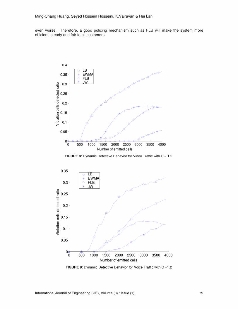
Ming-Chang Huang, Seyed Hossein Hosseini, K.Vairavan & Hui Lan
International Journal of Engineering (IJE), Volume (3) : Issue (1) 79
even worse. Therefore, a good policing mechanism such as FLB will make the system more efficient, steady and fair to all customers.
FIGURE 8: Dynamic Detective Behavior for Video Traffic with C = 1.2
0 500 1000 1500 2000 2500 3000 3500 40000
0.05
0.1
0.15
0.2
0.25
0.3
0.35
0.4
Number of emitted cells
Vio
latio
n c
ells
de
tecte
d r
atio
LB EWMAFLB JW
FIGURE 9: Dynamic Detective Behavior for Voice Traffic with C =1.2
0 500 1000 1500 2000 2500 3000 3500 40000
0.05
0.1
0.15
0.2
0.25
0.3
0.35
Number of emitted cells
Vio
latio
n c
ells
de
tecte
d r
atio
LB EWMAFLB JW

Ming-Chang Huang, Seyed Hossein Hosseini, K.Vairavan & Hui Lan
International Journal of Engineering (IJE), Volume (3) : Issue (1) 80
5.2.3 Performance Comparison between FLB and LB Systems
Finally, since the fuzzy leaky bucket shows improvement over leaky bucket, emphasized to compare the performance of these two policing mechanisms. By using the ON-OFF traffic model, packetized voice is simulated with parameters shown above in Table 2. Video traffic is simulated second. The generated traffic is fed through FLB and LB, when source does not respect to the negotiated parameters (cell violation), the simulation result shows that FLB is better than LB because FLB system modifies the token rate adaptively and decreases the need for buffer length. As seen in Figure 10~11, when ATM network switch node gets into congestion, i.e., traffic disobeys its traffic contract and sends more violated cells into network, FLB can deal with these violating cells in a smaller buffer size and still have the same controlling ability compared with LB. The figure is produced when C=1.4. It is because that at the same buffer size for both policing methods, FLB has a larger cell loss probability which means it allows less violated cells to enter the network by controlling for the leaking speed (token rate). FLB discards more violated cells with a higher cell loss probability (CLP=1) when traffic which does not follow the traffic contract.
10 20 30 40 50 60 70 80 9010
-2
10-1
100
Buffer size
Lo
ss
pro
ba
bili
ty
LB FLB
FIGURE 10: Performance of Cell Loss Probability (cell violation with C =1.4) vs. Buffer Size for Video Traffic
0 20 40 60 80 100 12010
-2
10-1
100
Buffer size
Lo
ss p
rob
ab
ility
LB FLB
FIGURE 11: Performance of Cell Loss Probability (cell violation with C =1.4) vs. Buffer Size for Voice Traffic

Ming-Chang Huang, Seyed Hossein Hosseini, K.Vairavan & Hui Lan
International Journal of Engineering (IJE), Volume (3) : Issue (1) 81
At the same time, for other performance characteristics, FLB can detect source violation with a shorter response time by decreasing the token rate. FLB is much better than LB in the dynamic detective behavior. It is clear that FLB shows a higher response capability for detecting and controlling violations in real time. Furthermore, the fuzzy logic would be combined with neural network to build an adaptive fuzzy control system and the relative parameters and fuzzy rules can be changed through adaptive learning to fit for different services. Till now, all the work is based on the analysis of the traffic and congestion control on the ATM switch node level. What is being done is to develop FLB policing mechanism based on the fuzzy logic combined with leaky bucket to protect and deal with the violating traffic in the UPC. The objective or goal of FLB policing mechanism is to lead the customers to obey their traffic contract, to prevent the violating traffic from getting into the main (backbone) network to violate network performance. In addition, all the analysis of this paper is on the cell level. Analysis on all level of the network, such as routing will greatly improve the network performance.
6. CONCLUSION
In this paper, a modified Leaky Bucket (LB) technique policing mechanism based on fuzzy logic system is presented to deal with the congestion control problem in ATM networks. Leaky Bucket mechanism (LB) is simple and easy to be implemented. However, its disadvantage is that the leaking rate is a constant so when there is mean cell rate violation, LB cannot reduce the high pressure for the main network. Therefore, a function is applied to control the leaking (token) rate. The main idea of FLB policing mechanism is to apply a fuzzy function to control the leaking rate. Fuzzy Leaky Bucket (FLB) identifies the traffic parameters and modifies the token rate based on the peak rate and the burst time, which characterize the source behavior. Due to the potential function offered by fuzzy logic, the FLB algorithm with an adaptive adjustment factor will balance the cell loss probability and the mean time delay, and also restrict the behavior of the traffic source to the traffic contract. From the above analysis and simulation results, FLB policing mechanism exhibits a good dynamic detective behavior, a high flexibility in selectivity performance and a fair capacity to meet the statistical properties of several B-ISDN traffic sources. The performance of the mechanism has been evaluated through several simulations and compared to some of the most popular policing mechanisms, such as the LB, JW and EWMA. The results show that the performance of FLB policer is much better than those of conventional policing mechanisms, in terms of both responsiveness and selectivity. The good performance is a result of the fuzzy feedback control mechanism since the token rate is adjusted on the fuzzy feedback control. EWMA can adjust the window size depending on the formula that reflects only a certain degree of few characteristics of cells in the network. However, FLB is based on the virtual leaky bucket and fuzzy logic. The mechanism monitors the real mean cell rate which gets into the network, then uses rules based fuzzy inference engine and defuzzification to adjust the token rate dynamically. Also, the control depends on its fuzzy characteristics. In the UPC parameter, mean cell rate is the average cell rate of the negotiated cells. It is detected in CAC; it’s a mean cell rate in the period between set-up and disconnecting a call connection. However,

Ming-Chang Huang, Seyed Hossein Hosseini, K.Vairavan & Hui Lan
International Journal of Engineering (IJE), Volume (3) : Issue (1) 82
UPC can only monitor the cell behavior periodically. For example, a period starts from one point in time and ends after a certain cell arrival. During this time period the mean cell rate may be greater than the negotiated cell rate, at that time the cell is violated. As long as time goes on, there is no cell coming in the next period, and the average cell rate may be lower than the negotiated cell rate. Consequently, that cell which violated at the beginning will not violate again. However, it takes a certain period of time to judge whether a cell is violated or not, but this time is not predetermined, and has a fuzzy characteristic. In addition, the relationship between virtual cell counter number N in virtual leaky bucket and cell number in the leaky bucket buffer X is also an un-determined fuzzy relationship. In the end, there are some final remarks that should be made about the prospects of the proposed approach. The problem should be solved with the choice of parameters describing the statistical properties of the various kinds of traffic. FLB mechanism shows a higher efficiency than others when the parameters are policed with the average cell rate for a long term. FLB is only good for less violation and quick response. What is important is to monitor and control the mean cell rate variation. This is why FLB may not be the best method for the cases in which the simulation time is very short. For the future work, an approach based on artificial intelligence techniques supported by the hypothesis with the neural network - Adaptive Neural-Fuzzy System may be improved to be more appropriate for the policing of other parameter characteristics of the traffic sources in the ATM network. Also, newer technologies such as genetic algorithm can be integrated to further enhance the performance of the hybrid systems. Overall, this paper emphasizes on ATM network fuzzy congestion control and policing. The fuzzy leaky bucket (FLB) method developed in this paper is good at cell violation controlling and shows better performance behaviors than other conventional policing mechanisms.
7. REFERENCES
1. G. Ascia, V. Catania, and Daniela Panno, "An Efficient Buffer Management Policy Based on an Integrated Fuzzy-GA Approach", IEEE INFOCOM 2: 1042-1048, 2002.
2. G. Ascia, V. Catania, and Daniela Panno. "A Fuzzy Buffer Management Scheme for ATM
and IP Networks", IEEE INFOCOM 3: 1539-1547, 2001. 3. Uyles Black, “ATM: Foundation for Broadband Networks”, Prentice Hall, 1995. 4. Uyles Black, “Emerging Communications Technologies 2nd Edition”, Prentice Hall, 1997. 5. Milena Butto, Elisa Cavallero and Alberto Tonietti, “Effectiveness of the “Leaky Bucket”
Policing Mechanism in ATM Networks”, IEEE Journal on Selected Areas in Communications, vol. 9, No. 3, pp335-341, April 1991.
6. Ray-Guang Cheng and Chung-Ju Chang, “Design of Fuzzy Traffic Controller for ATM
Networks”, IEEE/ACM Transactions on Networking, vol. 4, No. 3, pp460-469, June 1996. 7. Walter J. Goralski, “Introduction to ATM Networking”, McGraw Hall, Publishing House of
Electronics Industry, 1999. 8. Harry Heffes and David M. Lucantoni, “A Markov Modulated Characterization of Packetizd
Voice and Data Traffic and Related Statistical Multiplexer Performance”, IEEE Journal on Selected Areas in Communications, vol. Sac-4, No. 6, September Aug 1998.
9. Raj Jain, “The Art of Computer Systems Performance Analysis”, John Wiley & Sons, Inc.,
1991.

Ming-Chang Huang, Seyed Hossein Hosseini, K.Vairavan & Hui Lan
International Journal of Engineering (IJE), Volume (3) : Issue (1) 83
10. Jan Jantzen, “Design of Fuzzy Controllers”, Tech. Report no 98-E 864 (design), Technical University of Denmark, Department of Automation, Aug, 1998.
11. Somchai Lekcharoen, Chalida Chaochanchaikul and Chanintorn Jittawiriyanukoon. “A
design fuzzy control policing mechanisms on quality of service support in wireless networks”, Proceedings of the 3rd ACM International Conference on Mobile Technology, Applications & Systems (Mobility 06), pp1-6, Bangkok, Thailand, Oct. 25–27, 2006,
12. Somchai Lekcharoen and Chanintorn Jittawiriyanukoon. “QoS Sensitive Fuzzy Backoff
Schemes in Policing Mechanisms”, IEE Proceedings of the International Mobility Conference (MobiCon'05), 2005, 1--6.
13. Somchai Lekcharoen and Chanintorn Jittawiriyanukoon. “C. Deadlock of Avoidance Backoff
Schemes in Policing Mechanisms”, IEE Proceedings of the International Mobility Conference (MobiCon '05), 2005, pp.1--5.
14. Houming Liu, “Computer Networks”, Publishing House of Electronics Industry, 1997. 15. Shiwen Lu, “Data Communications and ATM Network”, Tsing Hua University Press, 1998. 16. Basil Maglaris, Dimitris Anastassiou, Prodip Sen, Gunnar Karlsson and John D. Robbins.
“Performance Models of Statistical Multiplexing in Packet Video Communications”, IEEE Transactions on Communications, vol. 36, No. 7, July 1988.
17. Hung T. Nguyen and Elbert A. Walker, “A First Course in Fuzzy Logic Second Edition”,
Chapman & Hall/CRC, 1999. 18. Naohisa Ohta, “Packet Video Modeling and Signal Processing”, Artech House, Inc., 1994. 19. Erwin P. Rathgeb, “Modeling and Performance Comparison of Policing Mechanism for ATM
Networks", IEEE Journal on Selected Areas in Communications, vol. 9, No. 3, pp325-333, April 1991.
20. Timothy J. Ross, “Fuzzy Logic with Engineering Applications”, McGraw-Hill, 1995. 21. R. Royand, S.S. Panwar, "Efficient Buffer Sharing inShared Memory ATM Systems with
Space Priority Traffic", IEEECommunications Letters 6: 162-164, 2002. 22.] Hiroshi Saito, Masatoshi Kawarasaki, Hiroshi Yamada, “An Analysis of Statistical
Multiplexing in an ATM Transport Network”, IEEE Journal on Selected Areas in Communications, vol. 9, No. 3, pp359-367, April 1991.
23. Mischa Schwartz, “Broadband Integrated Networks”, Prentice Hall, 1996. 24. William Stallings, “High Speed Networks TCP/IP and ATM Design Principles”, Prentice Hall,
1998. 25. Andrew S. Tanenbaum, “Computer Networks”, Prentice Hall Inc., 2004. 26. Hank B. Verbruggen and Robert Babuska, “Fuzzy Logic Control Advances in Applications”,
World Scientific Series in Robotics and Intelligent Systems – Vol. 23, World Scientific Publishing Co. Pte. Ltd., 1999.
27. Huigang Wang, “Computer System Simulation Theory and Applications,” University of
National Defense Technology Press, 1994.

Ming-Chang Huang, Seyed Hossein Hosseini, K.Vairavan & Hui Lan
International Journal of Engineering (IJE), Volume (3) : Issue (1) 84
28. Hiroshi Yamada, Shuichi Sumita, “A Traffic Measurement Method and its Application for Cell Loss Probability Estimation in ATM Network”, IEEE Journal on Selected Areas in Communications, vol. 9, No. 3, pp315-323, April 1991.
29. Huiling Zhao, Guohong Zhang, Lin Hu and Youkang Shi, “ATM, Frame Relay, IP Techniques
and Application”, Publishing House of Electronics Industry, 1998. 30. P Koutsakis and M. Paterakis, “Call-Admission-Control and traffic-policing mechanisms for
the transmission of videoconference traffic From MPEG-4 and H.263 video coders in wireless ATM networks”, IEEE transactions on vehicular technology, vol. 53, no. 5, 2004, 1525--1530.