interpolation-free fractional pixel motion estimation based on...

52

Interpolation-Free Fractional Pixel Motion Estimation Based on Data Trend Approximation

Chang-Uk JEONG and Hiroshi WATANABE

Abstract　　 Motion estimation can efficiently eliminate the temporal redundancy to achieve video compression. The computational complexity of a fractional pixel motion estimation（FME） module cannot be negligible, although such modules improve visual quality after the integer pixel motion estimation process. Most conventional FME methods include an interpolation procedure to form fractional pixel search points from information about the integer pixels. The interpolation, however, requires frequent memory access and a certain amount of processing time. In this paper, interpolation-free FME techniques using a data trend approximation are proposed. The proposed methods were implemented using the reference encoders of HEVC and H.264/AVC. The simulation results show that the proposed methods produce a similar or better performance than the existing FME methods

without the need for any additional search points.

Manuscript recieved 30th November 2013; revised 11th February 2014; accepted 25th February 2014

Graduate School of Global Information and Telecommunication Studies, Waseda University

1 IntroductionMobile network technologies such as the 3G, 4G,

and Long Term Evolution（LTE） wireless standards have made rapid progress. Nevertheless, the transmission of large amounts of multimedia data increases consumer traffic dramatically on both wireless and wired networks. Video compression standards, such as ISO/IEC MPEG-1 , MPEG-2 , MPEG-4 , ITU-T H.261 , H.263［1］, and H.264/AVC［2］, ［3］ also keep evolving. H.264/AVC is a state-of-the-art video compression standard for encoding and decoding video data using various advanced technologies. Although the advanced features allow it to encode video data more effectively compared with conventional methods, the increased computational complexity requires a certain level of CPU power to perform real-time video encoding, especially in mobile applications. The High Efficiency Video Coding （HEVC） standard, also known as H.265, has recently been jointly developed by ISO/IEC MPEG and ITU-T VCEG ［4］-［6］. HEVC can provide much higher video coding efficiency compared to H.264/AVC by halving the bitrates while maintaining a similar image quality, but this is achieved at the expense of a significant increase in computational complexity.

Generally, a video encoder is divided into three units: a temporal redundancy eliminator, a spatial redundancy eliminator, and an entropy encoder. The temporal redundancy eliminator estimates and extracts the motion of an object using the close correlation between neighboring

video frames, while information related to stationary objects or background is eliminated. As motion estimation（ME） is at the core of the temporal model, it occupies more than half of the total encoding time［7］. Thus, a great deal of research into fast ME has been conducted in an attempt to reduce the high computational complexity of the ME module.

Motion estimation methods can be classified into pixel recursive algorithms and block matching algorithms according to their elementary units, i.e., pixels or blocks. Block matching algorithms, in particular, have been adopted by many reference video encoders due to their low computational cost and robustness to errors. For example, the diamond search（DS）［8］, the hexagon-based search （HEXBS）［9］, the efficient three-step search（E3SS）［10］, the cross-diamond-hexagonal search（CDHS）［11］, the unsymmetrical-cross multi-hexagon-grid search （UMHexagonS）［12］, and the test zone search （TZS） implemented in the reference software such as JSVM［13］, JMVC［13］, and HM［14］ are fast block-based ME algorithms, developed to effectively reduce the computational complexity of the integer pixel ME （IME） module. Each of the existing IME algorithms has a different search strategy to satisfy both the accuracy of estimation and the search speed.

Most motion estimators follow the IME process with a fractional pixel ME（FME） process. The location of a moving object in a video sequence can be represented at fractional pixel, as well as integer pixel, precision. FME

53

GITS/GITI Research Bulletin 2013-2014

improves the image quality visibly, but requires higher computational complexity. The runtime of the FME module is over 30% of the total encoding time［7］. The conventional full fractional pixel search （FFPS）, also called the hierarchical fractional pixel search, is wasteful and inefficient owing to its fixed number of search points. In addition, an interpolation process （upsampling） must be performed to create the fractional pixel search area, which requires a high computational complexity and frequent memory access. To ameliorate these issues, techniques such as center-biased fractional pixel search （CBFPS）［12］, fast sub-pixel ME having lower computational complexity ［15］, quadratic prediction-based FME （QPFPS）［16］, and fast ME with interpolation-free sub-sample accuracy ［17］ have been developed. In this paper, interpolation-

free FME techniques based on data trend approximations are proposed. These techniques focus on performing FME without interpolation operations. In the experimental results, the performance of the proposed algorithms will be evaluated in terms of their peak signal-to-noise ratio （PSNR） and bitrate.

2 Mathematical Models2.1 Parabolic Models to Approximate Matching

ErrorsBlock-based ME evaluates the matching error cost

obtained by subtracting the candidate region from the current macroblock in order to find the best matched block within a search range in the reference frame. Equations （1）［15］, ［17］, （2）［15］, and （3）［15］, ［16］, have been used to model the matching error F（x, y） at fractional pixel resolution.

),( yxF98

276

254

23

22

221

cycycxcxcxycxycyxcyxc

++++++++=

（1）

6542

322

1),( cycxcycxycxcyxF +++++= （2）54

232

21),( cycycxcxcyxF ++++= （3）

In particular, the parabolic models in （1） and （2） require the matching errors of the nine adjacent search points at integer pixel resolution, as described in Fig. 1, to determine coefficients c1–c9 and c1–c6, respectively. In other words, if all nine matching error costs are not provided by the IME process, the estimation cannot be guaranteed. To fix this problem, a full search （FS） and an eight neighbor search （ENS） have been used for IME ［15］, ［17］. However, FS is very wasteful in terms of computational complexity, and the rectangular search pattern consisting of eight IME search points used in ENS is inefficient compared with the small diamond search pattern （SDSP） with five IME search points, illustrated in Fig. 1. SDSP has been applied to many fast IME algorithms due to its efficiency and simplicity

［8］–［14］. In addition, many powerful IME algorithms, including UMHexagonS in H.264/AVC, terminate the search process using SDSP in the final step. UMHexagonS occasionally determines the best position by checking only one search point using the early termination technique ［12］. The fast IME algorithms using SDSP, therefore, may not calculate the matching errors of the diagonal search points surrounding the best determined position. Fig. 2 shows the results of a simulation counting the number of known IME search points with their matching error. In Fig. 2, the percentage K x,y of each local position （x, y） can be obtained as follows:

100

IMEfor used smacroblock theofnumber totalThe

pointssearch known theofnumber The(%), ×=yxK （4）

In the simulation, UMHexagonS is used for IME with the QCIF test video sequence “Salesman” （100 frames） and the CIF sequence “Football” （100 frames）. These videos include small and large motion objects, respectively. As described in Fig. 2, the percentage K 0,0 of the known integer pixel search points of the center position （0,0）, which represents the local coordinates of the search point

Fig. 1 The five main integer pixel search points （H1, H2, C, V1, V2） and the four relatively unimportant search points （U）. The five main search points form the SDSP.

Fig. 2 Results of a simulation counting the number of known integer pixel search points with their matching error cost by performing UMHexagonS. （a） Percentages of known search points within a 3 × 3 range of the local position for the QCIF “Salesman” sequence. （b） Percentages for the CIF “Footbal l ” sequence.

　　　　　　　( a )　　　　　　　　　　　　　　(b )

54


corresponding to the best position with the lowest matching error, is always 100%, and the percentages （K-1,0, K1,0, K0,-1, K0,1） of the four positions forming the SDSP are also over 90%. In contrast, the four diagonal positions on the edge have low percentages （K-1,-1, K1,-1, K-1,1, K1,1） of about 7% and 40% for the “Salesman” and “Football” sequences, respectively. This means that the two models in （1） and （2） have difficulty working with powerful IME algorithms using SDSP. Accordingly, if a fast IME using SDSP was to be followed by the FME process based on （1） or （2）, it would cause an increase in the total encoding time and require some modifications to the fast IME module. The models in （1） and （2） are also unstable on the extension to the quarter pixel or less-than-one FME. This is because some matching errors at the outside half-pixel locations, e.g., （－0.5,－1）, must be additionally approximated after calculating the coefficients.

Contrary to the mathematical models discussed above, the parabolic model in （3） can be applied without any difficulties under state-of-the-art IME techniques because it needs only five IME matching errors, as described in Fig. 1, to determine the five coefficients c1–c5. This model can also be decomposed into two one-dimensional （1-D） parabolic models that approximate the horizontal and vertical matching errors separately, as described in the following equation:

)(,)( 322

1 yorxpcpcpcpF =++= （5）

As has been discussed ［16］, the minimum matching error cost F（p） can easily be found by differentiation with respect to x and y. When dF/dp ＝ 0, the x and y coordinates are regarded as the best prediction position （xb, y b）.

1

221 2

,02)(cc

pcpcpF b−

==+=′ （6）

The 1-D parabolic model uses only the three IME matching error costs, corresponding to （H1, C, H2） or （V1, C, V2）, to compute c1–c3, as derived in （7）［16］.

CcIIc

VorHIVorHICIIc

=+−=

==−+=

3

212

222111211

2/)(),(,2/)2(

（7）

The best predicted xb and yb coordinates are estimated independently of each other. Here, however, the 1-D parabolic model-based prediction has a serious fault, as shown below:

21

2,

1

22 >

−=>

cc

pifIC b （8）

Equation （8） is an abnormal case, and there is a contradiction because the matching error C at the local location （0, 0） always returns the lowest error cost in the IME. That is, the 1-D parabolic model-based prediction alone is not able to find the best prediction position at locations with pixel values greater than 0.5 or less than －0.5. This will have a serious impact on the FME process at quarter-pixel or less-than-one resolution. Moreover, if the matching error H1 or H2 is set to zero, denoting an unknown matching error, the 1-D parabolic graph tends to be concave down rather than concave up. As an alternative solution, to enhance the reconstruction PSNR performance, QPFPS ［16］ adopted an interpolation-based refinement procedure in its final search step, although this led to an increase in computational complexity.

2.2 Surface Modeling to Approximate Data TrendsThe parabolic models discussed in the previous

subsection can be extended to higher-order polynomial surface models to achieve more accurate prediction. However, higher-order polynomial functions require more computational complexity and IME matching error costs, and often result in unwanted undulations. Thus, different forms of error surface modeling from the above-mentioned parabolic models have been considered. Free-form surface modeling is used to describe the skin of a 3-D geometric element. The surfaces do not have rigid radial dimensions, unlike in parabolic surface modeling. Free-form splines include the following methods: Cardinal, Hermite, Bézier, and non-uniform rational B-spline （NURBS）. A Cardinal spline is a sequence of individual curves joined to form a larger curve, and a Hermite spline uses two points and two tangents to model a 2-D curve. Bézier splines, particularly in their quadratic and cubic forms, are widely used to model smooth curves. To model a quadratic Bézier curve, only three control points are required. The latest fast IME algorithms such as UMHexagonS terminate the final search step using SDSP with the five search points shown in Fig. 1 as the smallest search pattern. In particular, each of the IME search points （H1, C, H2） and （V1, C, V2） correspond to the three control points of a quadratic Bézier curve. A quadratic Bézier curve is also a parabolic segment, but it does not pass by all of the control points. Although the curve is not an interpolation between the control points, it can approximate the data trend. Hence, quadratic Bézier curve-based FME techniques are introduced. NURBS, which can be defined by degree, weighted control points, knot vector, and evaluation rules, is currently a very popular type of spline. To model a free-form curve with NURBS, the number of control points must be greater than or equal to four. NURBS is a generalization of B-splines and Bézier splines.

55


2.3 Quadratic Bézier CurveIn the 1-D parabolic model in （5）, the three IME

search points （H1, C, H2） or （V1, C, V2）, as shown in Fig. 1, are used to predict the best fractional pixel position at the horizontal or vertical location. As discussed in the previous subsection, quadratic Bézier curves are a natural choice for this problem, because the three IME search points correspond to the three control points of the quadratic Bézier curve. The quadratic Bézier curve algorithm can be explained by （9） and （10）. Equation （9） describes a generalization of the Bézier curve.

)!(!!

)1()(

)10(,)()(

,

0,

ininC

ttCtJ

ttJptP

in

iniinin

n

iini

−=

−=

≤≤=

−

=∑

（9）

where n denotes the degree of the Bézier curve, p0, p1, …, pn-1, pn are control points, and nCi is the binomial coefficient. While the parameter t moves from 0 to 1, the function P（t） traces a curve. Let the matching error costs corresponding to the local positions （x i , 0） and （0, y i） be Xi and Yi. Considering the coordinates for 1-D surface modeling, when xi or yi ＝ i-1, the IME search points （H1, C, H2） and （V1, C, V2） can be represented as {（x0, X0）, （x1, X1）, （x2,

X2）} and {（y0, Y0）, （y1, Y1）, （y2, Y2）}, respectively. At xi or yi ＝ mi and Xi or Yi ＝ Mi, each of the coordinates mi and Mi is entered separately as a control point pi. The quadratic Bézier curve given by the three control points （p0, p1, p2） is described in （10）, which forms the core of the proposed techniques.

221

20

02222

11121

20020

2

0,2

)1(2)1(

)1()1()1(

)()(

tpttptpttCpttCpttCp

tJptPi

ii

+−+−=

−×+−×+−×=

= ∑=

（10）

Fig. 3 shows examples of quadratic Bézier curves and the 1-D parabolic model. As shown, the quadratic Bézier curve does not pass by all three control points, but two points are always passed. The x or y coordinate with the lowest

matching error cost will be regarded as the best prediction position xb or yb. The best prediction position found by the quadratic Bézier curve, however, tends to be more biased toward x ＝－1 or 1 than that of the 1-D parabolic model, as illustrated in Fig. 3 （b）. Thus, a preprocessing algorithm is introduced to correct the one-directional bias.

3 Proposed Bézier Curve-Based FME3.1 Proposed Method 1

In this paper, three FME methods based on quadratic Bézier curves are proposed. The first method differentiates the quadratic Bézier curve in （10） to give:

)(2)2(2)( 10210 pppppttP −−+−=′ （11）

Let P（t）′ be zero. When （p0, p1, p2）＝（M0, M1, M2）, it is possible to obtain the optimum value of tb that minimizes the matching error cost, as shown below:

)2()(0)(2)2(2)(

21010

10210

ppppptpppppttP

b +−−==−−+−=′

（12）

As described in （13）, when （p0, p1, p2）＝（m0, m1, m2）＝（－1, 0, 1）, the best fractional pixel prediction position P（tb） can be found by substituting the above optimum tb for t in （10）.

12)1(2)1()( 221

20 −=+−+−= bbbbbb ttpttptptP （13）

Table 1 compares the fractional pixel motion vector （FMV） found by the 1-D parabolic model-based

prediction （1-D_PM） and that found by the proposed method （BÉZIER） at quarter-pixel resolution. The matching probabilities given refer to the agreement of the two methods with the best FMV found by FFPS. In the simulation, it is assumed that the FMV matching performance of FFPS is always the best. The QCIF “Salesman” sequence and the CIF “Football” sequence

are used as test input images. Both sequences consist of 100 frames. UMHexagonS is used for IME and returns the five neighboring IME matching errors. The best fractional pixel prediction positions determined by the two algorithms are subjected to quantization operations ［16］. Abnormal cases, such as the IME matching error H1 or H2 being unknown or zero, are not allowed, and the FME process for the macroblock is skipped in exceptional cases. If the x or y coordinate of the best FMV found by FFPS is equal to that found by a mathematical model-based prediction, it counts the number of matching FMVs in position |P |. As shown in Table 1 （A） and （B）, the 1-D parabolic model-based prediction can produce more accurate FMVs than the quadratic Bézier curve-based prediction. However, the 1-D parabolic model-based prediction can never find

Fig. 3 Examples of a 1-D parabolic model and a quadratic Bézier curve. （a） The two curves plotted using the three matching errors located at （-1, 5759）, （0, 1659）, （1, 5759）. （b） The curves at （-1, 5759）, （0, 1659）, （1, 3146）.

　　　　　　　( a )　　　　　　　　　　　　(b )

56


the best xb or yb located at |P |＞0.5, unlike the quadratic Bézier curve-based prediction. That is, compared with the 1-D parabolic model-based prediction, the quadratic Bézier curve approach provides higher robustness to large motions. It should be noted that, in general, macroblocks with larger motions result in higher distortion.

3.2 Proposed Method 2The second method involves predicting p1' in order to

pass close to all three control points. Thus, p 1' should be predicted such that p 1 can exist on the Bézier curve. As p1 is equal to P（t ＝ 0.5）, p1' can be computed as:

)4(21'

)21()

211(

21'2)

211()

21(

2011

221

201

pppp

ppppp

−−=

+−+−==

（14）

If p1 in （12） is replaced by p1', then the Bézier curve can pass through p1 as well as p0 and p2, as shown below:

)'2()'( 21010 ppppptb +−−= （15）

Finally, when （p0, p1, p2）＝（M0, M1, M2）, （16） is used to determine the best fractional pixel prediction position P（tb）. The result of the prediction is the same as that of the 1-D parabolic model-based prediction, although the approach is different. This second proposed method, however, can easily be extended to a third method.

)242()(12)( 21020 pppppttP bb +−−=−= （16）

3.3 Proposed Method 3: Determination of Adjusting Factors

As shown in Table 2, each location （x, y） corresponds to the five main IME search points （H1, H2, C, V1, V2）. Table 2（a） shows the average matching error costs at the

five IME search points for the QCIF sequence “Claire”（100 frames） and Table 2（b） shows the same information for the CIF sequence “Stefan” （100 frames）. In the simulation, the sum of absolute difference （SAD） criterion is used to calculate the matching errors for a given quantization parameter （QP） of 28 and rate-distortion optimized mode （RDO） of 1, based on the H.264/AVC JM version 12.4 reference software ［13］, ［18］. In the case of “Claire,” with reference to Fig. 3（a）, the prediction curves are almost symmetric about x ＝ 0. For the “Stefan” sequence, on the other hand, the horizontal search points （H1, C, H2） form slightly uneven curves, similar to Fig. 3（b）. That is, the simulation implies that the FMVs for “Claire” are more center-biased than those for “Stefan.” Actually, since “Claire” comprises stationary and small-motion objects,

most of the integer pixel motion vectors are distributed within the central area. Furthermore, for the quadratic Bézier curve, the following can be assumed:

First, the more similar the matching error H1 （V1） is to H2 （V2）, the closer the best prediction position is to the center. The best prediction position will also be similar to that of the 1-D parabolic model.

Second, the higher or lower H1 is compared to H2, the more the best prediction position is biased in one direction. That is, the best prediction position will be located farther away from that of the 1-D parabolic model.

Third, the farther H1 and H2 are from C, the closer the best prediction position is to the center. The best prediction position will also be similar to that of the 1-D parabolic model.

Finally, the closer H1 and H2 are to C, the more the best prediction position is biased in one direction. That is, the best prediction position will be located farther away from that of the 1-D parabolic model.

In the second proposed method, it is known that the shape of the quadratic Bézier curve can be determined by controlling the predicted control point p1', as illustrated in Fig. 4. The adjusting factors used in the third proposed method are described by the pseudo-code in Table 3. Each adjusting factor is composed according to certain assumptions. Let （p0, p1, p2）＝（M0, M1, M2）. As shown in Table 3, the variable D, which represents the original distance between p1 and p1', can be obtained by applying （14）, as used in the second method. The adjusting factor

Table 1 Fractional Pixel Motion Vector Matching Probability（%）

（a） QCIF “Salesman” Sequence

Method Position［0,±0.75］ |P| = 0 |P| = 0.25 |P| = 0.5 |P| = 0.75

1-D_PMx-coord. 44.928 49.969 28.606 14.598 00.000y-coord. 39.768 43.321 28.010 15.998 00.000

BÉZIERx-coord. 30.559 33.963 16.497 15.257 30.711y-coord. 27.329 30.046 15.285 14.616 27.359

（b） CIF “Football” Sequence

Method Position［0,±0.75］ |P| = 0 |P| = 0.25 |P| = 0.5 |P| = 0.75

1-D_PMx-coord. 28.673 50.725 23.179 15.063 00.000y-coord. 24.592 39.588 23.874 14.763 00.000

BÉZIERx-coord. 22.465 36.714 13.949 14.273 24.193y-coord. 18.278 25.977 13.483 14.364 25.168

Table 2 Average IME Matching Error Costs

（a） “Claire” （b） “Stefan”

(x, y) -1 0 1 (x, y) -1 0 1-1 – 122.100 – -1 – 311.212 –0 133.955 103.513 133.174 0 283.471 236.197 294.1311 – 121.288 – 1 – 308.656 –

57


AF 1 is based on the assumption that a higher ratio of p 0 to p 2 will lead to a bigger gap between p 1 and p 1'. The ratio of p 0＋p 2 to 2p 1 gives AF 2, which represents the relative difference between them. The critical value 1.5 in the second conditional sentence is used to determine the adjusting factor AF 3. The critical value is experimentally selected to be higher than AF 2＝1.29 computed by the matching errors （H1, C, H2） in Table 2（A）. If AF2 is less than the critical value, the relationship between p 0 and p 2 is preferred to that between p 0＋p 2 and p 1, in which case AF3 is AF1 multiplied by 10 determined by many tests. The last line of the pseudo-code shows that the position of p 1' is determined by applying D adjusted by AF3. The procedure of the third proposed method for obtaining the best prediction position xb or yb can be summarized as follows:

Step_1） The IME process for a prediction block is terminated and returns the IME matching error costs.

Step_2） The adjusting factors for controlling p 1' are determined by the pseudo-code described in Table 3.

Step_3） The predicted p 1' is entered in （15）, and then the optimum tb is computed.

Step_4） The best prediction position is found by applying the optimum tb in （13）. The best prediction position is quantized according to a previously reported method ［16］.

3.4 Proposed Method 3: Modification for HEVCHEVC is the latest video compression standard

suitable for high-resolution video formats such as WQXGA, 4K, and 8K. In place of the 16 × 16 macroblock adopted in H.264/AVC, HEVC is based on a coding tree unit （CTU） with a maximum size of 64 × 64. The CTU consists of three blocks: a luma coding tree block （CTB）, two chroma CTBs, and syntax elements. Since larger CTB

sizes generally produce a lower bitrate, large CTB sizes have a strong influence on the coding efficiency with high-resolution video. Each CTB can be split into multiple coding units （CUs）. The CU also consists of three blocks: a luma coding block （CB）, two chroma CBs, and syntax elements. Each CU is again partitioned into prediction units （PUs） and a quadtree of transform units （TUs）. The CU level determines the inter or intra prediction mode, and each CB can be split into prediction blocks （PBs）. Larger blocks tend to lead to higher matching error costs.

Therefore, the adjusting factor AF 3 described in Table 3 is modified to suit the HEVC test model （HM） version 12.0 reference software ［14］, as shown below:

AF3 ＝ if （4.0 ＞ AF2） then AF1, else AF2 – 2.0 （17）

HEVC utilizes 7- or 8-tap interpolation filters for the motion vector refinement process at quarter-pixel resolution, whereas H.264/AVC performs a two-step interpolation: 6-tap interpolation filtering of half-pixel resolution positions followed by a bilinear interpolation for quarter-pixel resolution positions. Both HEVC and H.264/AVC refine the motion vectors at the quarter-pixel resolution; thus, the quantization process of ［16］ is also used in the final prediction step of the third proposed method in HEVC.

4 Experimental Results4.1 Simulation Results Based on H.264/AVC

The proposed techniques have been implemented in H.264/AVC JM 12.4 on the Windows 7 64-bit OS platform with an Intel i5 [email protected] GHz, and HEVC HM 12.0 on the Windows 7 64-bit OS platform with an Intel i7 [email protected] GHz. Based on the H.264/AVC JM 12.4, the simulation was conducted using the default settings, i.e., search range ＝ 16, QPs ＝ 20, 24, 28, and 32, and RDO ＝ 1 under the baseline profile. As implemented in JM, UMHexagonS is used for fast IME. The performance of the proposed methods （METHOD_1–3） is evaluated by comparison with that of CBFPS and the 1-D parabolic model-based prediction （1-D_PM） in terms of PSNR and bitrate. The computational complexity can be compared in terms of the total motion estimation time （MET） and the average number of fractional pixel search points per block （FSP）. CBFPS is chosen as one of the most popular interpolation-based FME algorithms. As defined in JM, if a macroblock type is less than or equal to 3, UMHexagonS is performed, followed by FFPS rather than CBFPS for FME. The rule, therefore, is applied to all the FME methods for fair comparison, and the fractional pixel search points used in FFPS are not counted. In

Fig. 4 Determination of the Bézier curve by controlling p1'.

Table 3 Pseudo-Code for the Third Proposed Method

D ＝（0.5 × （4.0 × p1 － p0 － p2））－ p1AF1 ＝ if （p0 ＞ p2） then （p0 / p2） – 1.0, else （p2 / p0） – 1.0AF2 ＝（p0 ＋ p2） / （2.0 × p1）AF3 ＝ if （1.5 ＞ AF2） then AF1 × 10.0, else AF2 – 1.0p1' ＝ p1 ＋（D × AF3）

58


addition, the mathematical model-based methods have been implemented in the IME module of JM. However, because the PSNR and bitrate in IME are measured, the computational complexity will only be mentioned briefly. The six sequences used in the test are as follows: QCIF （176×144） “Claire” and “Salesman,” CIF （352×288） “Football,” “News,” “Stefan,” and “Table.” Each sequence

includes different types of motion, which can be classified as small, middling, and large motion. The number of frames to be encoded is 100 at 30 Hz.

As l i s ted in Tables 4–8 , the average qual i t y performance of METHOD_3 at each QP is better than that of 1-D_PM. The average PSNR degradation of 0.016 with respect to CBFPS is lower than the 0.025 attained by 1-D_PM. In particular, the average PSNR drop at each QP ＝ 28 and QP ＝ 32 is 0.003, which means that the quality is very close to that of CBFPS. In terms of computational complexity, METHOD_3 has no use for FSPs, whereas CBFPS requires at least five. METHOD_1–3 and 1-D_PM achieve an average MET reduction of 17.198%, 17.824%, 16.894%, and 17.033%, respectively, with respect to CBFPS. The computational load of METHOD_3 can also be reduced from about 11% to 30% compared with CBFPS. When METHOD_3 is directly implemented in the IME module of JM, the average MET reduction is about 46%, whereas the quality is expected to degrade a little compared with that in the FME module with the above simulation conditions. The bitrate comparisons in Tables 4–8 show that METHOD_3 is competitive with 1-D_PM. The bitrate of METHOD_3 shows an average increase of less than 0.081% with respect to 1-D_PM. On the other hand, the average PSNR degradation of 0.022 for METHOD_1 with respect to CBFPS is lower than that of 1-D_PM, but the bitrate increase compared with 1-D_PM averages about 0.2%. The performance of METHOD_2 is equal to that of 1-D_PM with similar computational complexity.

4.2 Simulation Results Based on HEVCBased on the HEVC HM 12.0, the simulation was

carried out under the main profile using the following configuration parameters: group of pictures （GOP） size ＝ 4, intra period ＝－1, search range ＝ 64, and decoding refresh type ＝ 0. The four QPs used in this test are 22, 27, 32, and 37. As adopted in HM, TZS is selected as a fast IME search algorithm. As mentioned above, the results of the simulation conducted for H.264/AVC JM 12.4 show that the performances of METHOD_1 and METHOD_2 are very similar or equal to that of 1-D_PM, whereas METHOD_3 is better than 1-D_PM for most of the test sequences at each QP. In this simulation based on HM, the performance of METHOD_3 is

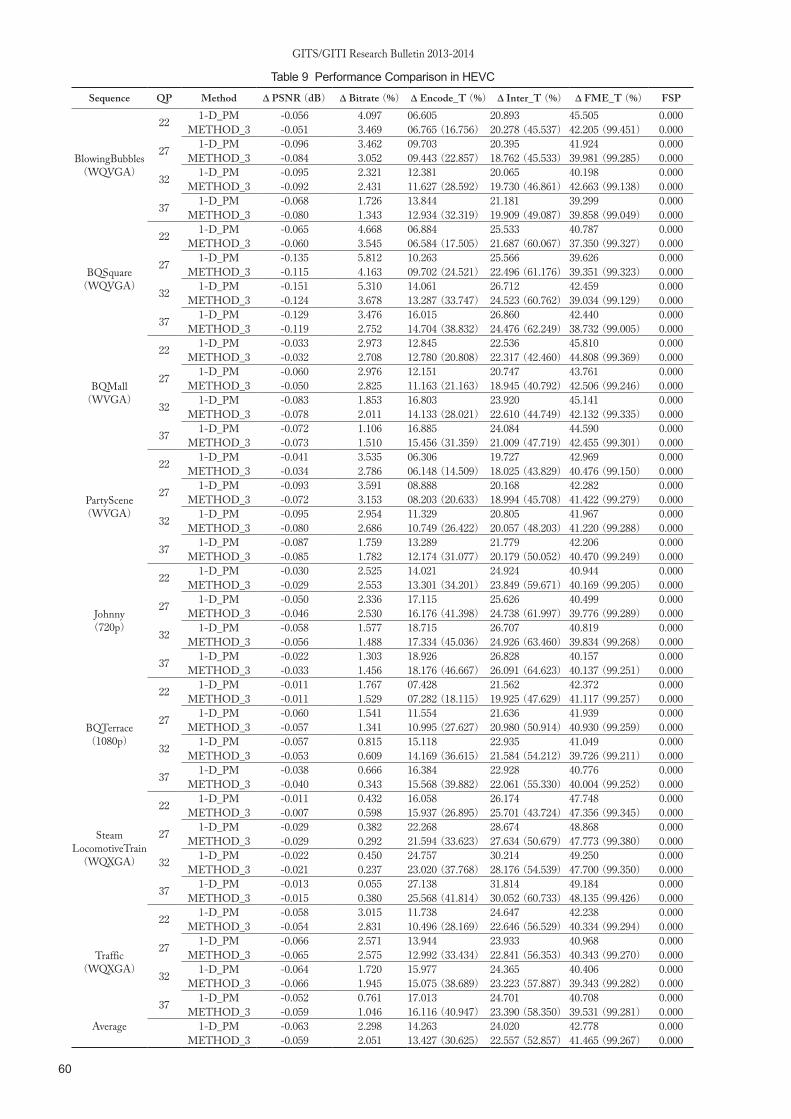
therefore directly compared with that of 1-D_PM. FFPS implemented in HM is selected as the anchor FME algorithm. The performance comparisons are shown in Tables 9 and 10, where Δ PSNR represents the PSNR difference between 1-D_PM and FFPS, or METHOD_3 and FFPS, which means a PSNR degradation with respect to FFPS; Δ Bitrate denotes the bitrate increase in percentage with respect to FFPS; and Δ Encode_T, Δ Inter_T, and Δ FME_T represent the total encoding time reduction, inter prediction time reduction, and FME time reduction in percentage with respect to FFPS, respectively. The Bjøntegaard delta （BD） PSNR （BD-PSNR） and bitrate （BD-Bitrate）［19］ are used to evaluate the objective differences between the two rate-distortion curves. Similar to METHOD_3 implemented in JM, METHOD_3 was also implemented without using an interpolation process （upsampling） in the FME module of HM. Since the HM module without upsampling does not accurately measure the PSNR and bitrate, only the complexity reduction is reported; Table 9 lists these values in parentheses. The eight sequences used in the test are as follows: WQVGA （416 × 240） “BlowingBubbles” （50 Hz） and “BQSquare” （60 Hz）, WVGA （832 × 480） “BQMall” （60 Hz） and “PartyScene” （50 Hz）, 720p （1280 × 720） “Johnny” （60 Hz）, 1080p （1920 × 1080） “BQTerrace”（60 Hz）, WQXGA （2560 × 1600） “SteamLocomotiveTrain” （60 Hz）, and “Traffic” （30 Hz）. The number of frames to be encoded is 100 for each sequence.

As shown in Table 9, the average PSNR and bitrate performances of METHOD_3 are better than those of 1-D_PM. The PSNR degradation for most of the test sequences against four QPs is lower compared with 1-D_PM. The BD-PSNR of METHOD_3 shown in Table 10 is also higher than that of 1-D_PM. In particular, the PSNR value for “SteamLocomotiveTrain” is considerably close to that of FFPS, whereas the bitrate increase with respect to FFPS is negligible and lower than that of 1-D_PM. The bitrate for the WQVGA and WVGA sequences shows a much lower increase compared with 1-D_PM. Fig. 5 shows the rate-distortion （R-D） curves for the eight sequences with QPs ＝ 22, 27, 32, and 37. The R-D curves show that the R-D performances for the WQVGA and WVGA sequences are better than with 1-D_PM, and the performances for the 720p, 1080p, and WQXGA sequences are close to that of FFPS. In terms of computational complexity, METHOD_3 and 1-D_PM do not require any FSPs, whereas FFPS always uses 16 FSPs. As shown in Table 9, the total encoding time of METHOD_3 can be reduced from about 6% to 25%, and the average FME time reduction is 41.465%, with respect to FFPS. When METHOD_3 is implemented without upsampling in the encoder, the encoding time can be dramatically reduced

59


Table 8 Average Values with Respect to CBFPS （QP=20, 24, 28, 32）Method Δ PSNR （dB） Δ Bitrate Increase （%）Δ MET Reduction （%） FSP1-D_PM -0.025 4.333 17.033 0.000

METHOD_1 -0.022 4.537 17.198 0.000METHOD_2 -0.025 4.333 17.824 0.000METHOD_3 -0.016 4.414 16.894 0.000

Table 4 Performance Comparison in H.264/AVC （QP=20）

Sequence Method PSNR （dB）

Bitrate （kbps）

MET （ms） FSP

Claire（QCIF）

CBFPS 45.713 109.838 7091 4.9041-D_PM 45.674 116.882 5174 0.000

METHOD_1 45.676 116.561 5646 0.000METHOD_2 45.674 116.882 5340 0.000METHOD_3 45.672 116.225 5918 0.000

Salesman（QCIF）

CBFPS 42.217 180.509 7009 5.0851-D_PM 42.175 195.919 5679 0.000


Football（CIF）

CBFPS 43.595 4009.248 62397 8.5891-D_PM 43.564 4103.251 52649 0.000


News（CIF）

CBFPS 43.651 669.869 31116 5.2571-D_PM 43.605 703.241 24109 0.000


Stefan（CIF）

CBFPS 43.299 4244.916 44922 6.8711-D_PM 43.264 4325.671 38559 0.000


Table（CIF）

CBFPS 42.699 2918.530 42427 7.3701-D_PM 42.640 3045.521 35257 0.000


Table 5 Performance Comparison in H.264/AVC（QP=24）


Bitrate （kbps）

MET （ms） FSP

Claire（QCIF）

CBFPS 42.715 61.224 7324 4.7951-D_PM 42.732 64.267 5822 0.000


Salesman（QCIF）

CBFPS 38.947 103.531 7708 5.1931-D_PM 38.907 113.136 6331 0.000


Football（CIF）

CBFPS 40.464 2637.679 62989 8.1371-D_PM 40.464 2711.268 53192 0.000


News（CIF）

CBFPS 41.135 390.722 31177 5.0921-D_PM 41.101 410.918 25670 0.000


Stefan（CIF）

CBFPS 39.844 2560.536 45628 6.6301-D_PM 39.810 2631.269 39913 0.000


Table（CIF）

CBFPS 39.253 1591.188 45107 7.0751-D_PM 39.212 1667.450 35327 0.000




Bitrate （kbps）

MET （ms） FSP

Claire（QCIF）

CBFPS 39.716 33.324 8025 4.6601-D_PM 39.676 34.181 6292 0.000


Salesman（QCIF）

CBFPS 35.799 59.638 9463 5.2861-D_PM 35.763 63.914 7198 0.000


Football（CIF）

CBFPS 37.576 1730.412 62116 7.4931-D_PM 37.563 1772.098 53280 0.000


News（CIF）

CBFPS 38.517 230.314 31024 4.9201-D_PM 38.500 241.286 26357 0.000


Stefan（CIF）

CBFPS 36.452 1441.358 46835 6.4591-D_PM 36.436 1502.765 39502 0.000


Table（CIF）

CBFPS 36.250 861.838 45089 6.5911-D_PM 36.225 903.982 38780 0.000




Bitrate （kbps）

MET （ms） FSP

Claire（QCIF）

CBFPS 36.753 18.552 8261 4.5351-D_PM 36.749 18.607 7019 0.000


Salesman（QCIF）

CBFPS 32.700 33.643 9604 5.2941-D_PM 32.655 34.548 9262 0.000


Football（CIF）

CBFPS 34.581 1068.910 66632 6.9211-D_PM 34.582 1097.966 54539 0.000


News（CIF）

CBFPS 35.626 135.864 32857 4.8261-D_PM 35.627 140.616 29296 0.000


Stefan（CIF）

CBFPS 32.796 671.957 47462 6.3721-D_PM 32.787 715.740 41516 0.000


Table（CIF）

CBFPS 33.252 438.204 53105 5.9791-D_PM 33.228 455.419 40769 0.000


60


Table 9 Performance Comparison in HEVC

Sequence QP Method Δ PSNR （dB） Δ Bitrate （%） Δ Encode_T （%） Δ Inter_T （%） Δ FME_T （%） FSP

BlowingBubbles（WQVGA）

22 1-D_PM -0.056 4.097 06.605 20.893 45.505 0.000METHOD_3 -0.051 3.469 06.765 （16.756） 20.278 （45.537）42.205 （99.451） 0.000

27 1-D_PM -0.096 3.462 09.703 20.395 41.924 0.000METHOD_3 -0.084 3.052 09.443 （22.857） 18.762 （45.533）39.981 （99.285） 0.000

32 1-D_PM -0.095 2.321 12.381 20.065 40.198 0.000METHOD_3 -0.092 2.431 11.627 （28.592） 19.730 （46.861）42.663 （99.138） 0.000

37 1-D_PM -0.068 1.726 13.844 21.181 39.299 0.000METHOD_3 -0.080 1.343 12.934 （32.319） 19.909 （49.087）39.858 （99.049） 0.000

BQSquare（WQVGA）

22 1-D_PM -0.065 4.668 06.884 25.533 40.787 0.000METHOD_3 -0.060 3.545 06.584 （17.505） 21.687 （60.067）37.350 （99.327） 0.000

27 1-D_PM -0.135 5.812 10.263 25.566 39.626 0.000METHOD_3 -0.115 4.163 09.702 （24.521） 22.496 （61.176）39.351 （99.323） 0.000

32 1-D_PM -0.151 5.310 14.061 26.712 42.459 0.000METHOD_3 -0.124 3.678 13.287 （33.747） 24.523 （60.762）39.034 （99.129） 0.000

37 1-D_PM -0.129 3.476 16.015 26.860 42.440 0.000METHOD_3 -0.119 2.752 14.704 （38.832） 24.476 （62.249）38.732 （99.005） 0.000

BQMall（WVGA）

22 1-D_PM -0.033 2.973 12.845 22.536 45.810 0.000METHOD_3 -0.032 2.708 12.780 （20.808） 22.317 （42.460）44.808 （99.369） 0.000

27 1-D_PM -0.060 2.976 12.151 20.747 43.761 0.000METHOD_3 -0.050 2.825 11.163 （21.163） 18.945 （40.792）42.506 （99.246） 0.000

32 1-D_PM -0.083 1.853 16.803 23.920 45.141 0.000METHOD_3 -0.078 2.011 14.133 （28.021） 22.610 （44.749）42.132 （99.335） 0.000

37 1-D_PM -0.072 1.106 16.885 24.084 44.590 0.000METHOD_3 -0.073 1.510 15.456 （31.359） 21.009 （47.719）42.455 （99.301） 0.000

PartyScene（WVGA）

22 1-D_PM -0.041 3.535 06.306 19.727 42.969 0.000METHOD_3 -0.034 2.786 06.148 （14.509） 18.025 （43.829）40.476 （99.150） 0.000

27 1-D_PM -0.093 3.591 08.888 20.168 42.282 0.000METHOD_3 -0.072 3.153 08.203 （20.633） 18.994 （45.708）41.422 （99.279） 0.000

32 1-D_PM -0.095 2.954 11.329 20.805 41.967 0.000METHOD_3 -0.080 2.686 10.749 （26.422） 20.057 （48.203）41.220 （99.288） 0.000

37 1-D_PM -0.087 1.759 13.289 21.779 42.206 0.000METHOD_3 -0.085 1.782 12.174 （31.077） 20.179 （50.052）40.470 （99.249） 0.000

Johnny（720p）

22 1-D_PM -0.030 2.525 14.021 24.924 40.944 0.000METHOD_3 -0.029 2.553 13.301 （34.201） 23.849 （59.671）40.169 （99.205） 0.000

27 1-D_PM -0.050 2.336 17.115 25.626 40.499 0.000METHOD_3 -0.046 2.530 16.176 （41.398） 24.738 （61.997）39.776 （99.289） 0.000

32 1-D_PM -0.058 1.577 18.715 26.707 40.819 0.000METHOD_3 -0.056 1.488 17.334 （45.036） 24.926 （63.460）39.834 （99.268） 0.000

37 1-D_PM -0.022 1.303 18.926 26.828 40.157 0.000METHOD_3 -0.033 1.456 18.176 （46.667） 26.091 （64.623）40.137 （99.251） 0.000

BQTerrace（1080p）

22 1-D_PM -0.011 1.767 07.428 21.562 42.372 0.000METHOD_3 -0.011 1.529 07.282 （18.115） 19.925 （47.629）41.117 （99.257） 0.000

27 1-D_PM -0.060 1.541 11.554 21.636 41.939 0.000METHOD_3 -0.057 1.341 10.995 （27.627） 20.980 （50.914）40.930 （99.259） 0.000

32 1-D_PM -0.057 0.815 15.118 22.935 41.049 0.000METHOD_3 -0.053 0.609 14.169 （36.615） 21.584 （54.212）39.726 （99.211） 0.000

37 1-D_PM -0.038 0.666 16.384 22.928 40.776 0.000METHOD_3 -0.040 0.343 15.568 （39.882） 22.061 （55.330）40.004 （99.252） 0.000

SteamLocomotiveTrain（WQXGA）

22 1-D_PM -0.011 0.432 16.058 26.174 47.748 0.000METHOD_3 -0.007 0.598 15.937 （26.895） 25.701 （43.724）47.356 （99.345） 0.000

27 1-D_PM -0.029 0.382 22.268 28.674 48.868 0.000METHOD_3 -0.029 0.292 21.594 （33.623） 27.634 （50.679）47.773 （99.380） 0.000

32 1-D_PM -0.022 0.450 24.757 30.214 49.250 0.000METHOD_3 -0.021 0.237 23.020 （37.768） 28.176 （54.539）47.700 （99.350） 0.000

37 1-D_PM -0.013 0.055 27.138 31.814 49.184 0.000METHOD_3 -0.015 0.380 25.568 （41.814） 30.052 （60.733）48.135 （99.426） 0.000

Traffic（WQXGA）

22 1-D_PM -0.058 3.015 11.738 24.647 42.238 0.000METHOD_3 -0.054 2.831 10.496 （28.169） 22.646 （56.529）40.334 （99.294） 0.000

27 1-D_PM -0.066 2.571 13.944 23.933 40.968 0.000METHOD_3 -0.065 2.575 12.992 （33.434） 22.841 （56.353）40.343 （99.270） 0.000

32 1-D_PM -0.064 1.720 15.977 24.365 40.406 0.000METHOD_3 -0.066 1.945 15.075 （38.689） 23.223 （57.887）39.343 （99.282） 0.000

37 1-D_PM -0.052 0.761 17.013 24.701 40.708 0.000METHOD_3 -0.059 1.046 16.116 （40.947） 23.390 （58.350）39.531 （99.281） 0.000

Average 1-D_PM -0.063 2.298 14.263 24.020 42.778 0.000METHOD_3 -0.059 2.051 13.427 （30.625） 22.557 （52.857）41.465 （99.267） 0.000

61


from about 14% to 46% with an FME time reduction of about 99%. METHOD_3 with and without upsampling achieves an average encoding time of 13.427% and 30.625%, respectively. METHOD_3 also has a similar complexity as 1-D_PM.

5 ConclusionThe recently released HEVC standard will achieve a

much more efficient compression performance for high-

resolution video formats beyond HDTV, as compared to H.264/AVC. Owing to a significantly increased computational complexity, however, additional costs will be incurred because the real-time encoder is implemented on consumer electronics devices, particularly mobile devices. In this paper, the proposed techniques focus on reducing the complexity. The proposed low-complexity interpolation-free techniques were developed to achieve a similar rate-distortion performance as interpolation-based FME. Moreover, the simplicity of the algorithm will make it suitable for hardware implementation. It can be directly implemented in the IME module, and easily extended to 1/8 or 1/16 pixel-resolution ME.

AcknowledgementThis paper is a part of the outcome of research

performed under a Waseda University Grant for Special Research Projects （Project number: 2013A-6324）.

References

［1］ K. R. Rao and J. J. Hwang, Techniques and Standards for Image, Video and Audio Coding, Englewood Cliffs, NJ: Prentice Hall, 1996.

［2］ T. Wiegand, G. J. Sullivan, and A. Luthra, Draft ITU-T Recommendation and Final Draft International Standard of Joint Video Specif ication （ITU-T Rec. H.264 | ISO/IEC 14496-10 AVC）, Joint Video Team （JVT） of ISO/IEC MPEG and ITU-T VCEG, document JVT-G050r1, 8th Meeting, Geneva, Switzerland, May 2003.

［3］ T. Wiegand, G. J. Sullivan, G. Bjøntegaard, and A. Luthra, “Overview of the H.264/AVC video coding standard,”

IEEE Trans. Circuits Syst. Video Technol., vol. 13, no. 7, pp. 560–576, Jul. 2003.

［4］ B. Bross, W.-J. Han, J.-R. Ohm, G. J. Sullivan, Y.-K. Wang, and T. Wiegand, High Eff iciency Video Coding （HEVC） Text Specif ication Draft 10 （for FDIS & Last Call）, Joint Collaborative Team on Video Coding （JCT-VC） of ITU-T SG 16 WP 3 and ISO/IEC JTC 1/SC 29/WG 11, document JCTVC-L1003, 12th Meeting, Geneva, CH, Jan. 2013.

［5］ G. J. Sullivan, J.-R. Ohm, W.-J. Han, and T. Wiegand, “Overview of the High Efficiency Video Coding （HEVC）

standard,” IEEE Trans. Circuits Syst. Video Technol., vol. 22, no. 12, pp. 1649–1668, Dec. 2012.

［6］ F. Bossen, B. Bross, K. Sühring, and D. Flynn, “HEVC complexity and implementation analysis,” IEEE Trans. Circuits Syst. Video Technol., vol. 22, no. 12, pp. 1685–1696, Dec. 2012.

［7］ Y.-W. Huang, B.-Y. Hsieh, S.-Y. Chien, S.-Y. Ma, and L.-G. Chen, “Analysis and complexity reduction of multiple reference frames motion estimation in H.264/AVC,” IEEE Trans. Circuits Syst. Video Technol., vol. 16, no. 4, pp. 507–522, Apr. 2006.

［8］ S. Zhu and K.-K. Ma, “A new diamond search algorithm for fast block matching motion estimation,” IEEE Trans. Image Process., vol. 9, no. 2, pp. 287–290, Feb. 2000.

［9］ C. Zhu, X. Lin, and L.-P. Chau, “Hexagon-based search

Table 10 Bjøntegaard Delta Performance Comparison in HEVC

Sequence BD-PSNR （dB） BD-Bitrate （%）1-D_PM METHOD_3 1-D_PM METHOD_3

BlowingBubbles -0.197 -0.183 5.432 4.992BQSquare -0.323 -0.252 8.902 6.874BQMall -0.160 -0.154 4.030 3.890

PartyScene -0.218 -0.188 5.314 4.560Johnny -0.087 -0.088 3.969 3.959

BQTerrace -0.075 -0.069 4.285 3.941SteamLocomoti_ -0.030 -0.030 1.549 1.496

Traffic -0.126 -0.129 4.213 4.332Average -0.152 -0.137 4.712 4.255

(h) “Tra�c”

(a) “BlowingBubbles” (b) “BQSquare”

(c) “BQMall” (d) “PartyScene”

(e) “Johnny” (f) “BQTerrace”

(g) “SteamLocomotiveTrain”

Fig. 5 Rate-distortion curves for the sequences with QPs ＝22, 27, 32, and 37 in HEVC.

62


pattern for fast block motion estimation,” IEEE Trans. Circuits Syst. Video Technol., vol. 12, pp. 349–355, May 2002.

［10］ X. Jing and L.-P. Chau, “An efficient three-step search algorithm for block motion estimation,” IEEE Trans. Multimedia., vol. 6, no. 3, pp. 435–438, Jun. 2004.

［11］ C.-H. Cheung and L.-M. Po, “Novel cross-diamond-hexagonal search algorithms for fast block motion estimation,” IEEE Trans. Multimedia., vol. 7, no. 1, pp. 16–22, Feb. 2005.

［12］ Z. Chen, J. Xu, Y. He, and J. Zheng, “Fast integer-pel and fractional-pel motion estimation for H.264/AVC,” J. Vis. Commun. Image R., vol. 17, pp. 264–290, Apr. 2006.

［13］ Reference Software for ITU-T H.264 Advanced Video Coding, ITU-T Rec. H.264.2, ITU-T and ISO/IEC JTC 1, Edition 1: Mar. 2005, Edition 2: Jun. 2008, Edition 3: Jun. 2010, Edition 4: Jan. 2012.

［14］ F. Bossen, D. Flynn, and K. Sühring, High Eff iciency Video Coding Test Moel 12 （HM 12） Reference Software, Joint Collaborative Team on Video Coding （JCT-VC） of ITU-T SG16 WP3 and ISO/IEC JTC1/SC29/WG11, document JCTVC-N1010, 14th Meeting, Vienna, AT, Jul. 2013.

［15］ J. W. Suh and J. Jeong, “Fast sub-pixel motion estimation techniques having lower computational complexity,” IEEE Trans. Consumer Electron., vol. 50, pp. 968–973, Aug. 2004.

［16］ J.-F. Chang and J.-J. Leou, “A quadratic prediction based fractional-pixel motion estimation algorithm for H.264,” J. Vis. Commun. Image R., vol. 17, pp. 1074–1089, Oct. 2006.

［17］ S. Dikbas, T. Arici, and Y. Altunbasak, “Fast motion estimation with interpolation-free sub-sample accuracy,” IEEE Trans. Circuits Syst. Video Technol., vol. 20, no. 7, pp. 1047–1051, Jul. 2010.

［18］ A. M. Tourapis, A. Leontaris, K. Sühring, and G. J. Sullivan, H.264/MPEG-4 AVC Reference Software Manual, ISO/IEC JTC1/SC29/WG11 and ITU-T SG16 Q.6, document JVT-X072, 24th Meeting, Geneva, CH, Jun. 2007.

［19］ G. Bjøntegaard, Calculation of Average PSNR Dif ferences be t ween RD Cur ve s , ITU-T SG16 Q .6 , document VCEG-M33, 13th Meeting, Austin, TX, Apr. 2001.

interpolation-free fractional pixel motion estimation based on...

Documents