Portland State University Portland State University

PDXScholar PDXScholar

Dissertations and Theses Dissertations and Theses

Spring 6-28-2013

Interspecific variation in leaf-level biogenic Interspecific variation in leaf-level biogenic

emissions of the Bambuseae emissions of the Bambuseae

Andrea Natalie Melnychenko Portland State University

Follow this and additional works at: https://pdxscholar.library.pdx.edu/open_access_etds

Part of the Atmospheric Sciences Commons, Biology Commons, and the Plant Biology Commons

Let us know how access to this document benefits you.

Recommended Citation Recommended Citation Melnychenko, Andrea Natalie, "Interspecific variation in leaf-level biogenic emissions of the Bambuseae" (2013). Dissertations and Theses. Paper 1031. https://doi.org/10.15760/etd.1031

This Thesis is brought to you for free and open access. It has been accepted for inclusion in Dissertations and Theses by an authorized administrator of PDXScholar. Please contact us if we can make this document more accessible: pdxscholar@pdx.edu.

Interspecific variation in leaf-level biogenic emissions

of the Bambuseae

by

Andrea Natalie Melnychenko

A thesis submitted in partial fulfillment of the requirements for the degree of

Masters of Science in

Biology

Thesis Committee: Todd N. Rosenstiel, Chair

Sarah Eppley Mitch Cruzan

Portland State University 2013

i

Abstract 1

Plants emit a diverse range of biogenic volatile organic compounds (BVOCs) into the 2

atmosphere, of which isoprene is the most abundantly emitted. Isoprene significantly 3

affects biological and atmospheric processes, but the range of isoprene and BVOCs 4

present in bamboos has not been well characterized. In this thesis I explore the range of 5

isoprene emission found in bamboos and relate it to plant morphological and 6

physiological characteristics. In addition, I measure and relate the entire suite of BVOCs 7

present in the bamboos to their fundamental isoprene emission rate. 8

Interspecific variation in isoprene emission documented in a comprehensive survey of 9

bamboos. Two groups of bamboo species were measured in the greenhouse and the field. 10

Elevated photosynthetic rate was significantly correlated with isoprene emission. In the 11

field, dark respiration rate was highest in bamboos that made the least amount of 12

isoprene. The total BVOC suite was significantly influenced by whether or not leaf-level 13

isoprene emission was present. I conclude that bamboos vary with regard to physiology, 14

morphology, and total BVOC suite and that isoprene emission is correlated with these 15

changes, and introduce the bamboos as a novel system for studying the impacts of 16

isoprene emission. 17

18

ii

Acknowledgements 1

This thesis is dedicated to the people I have loved and who have loved me throughout this 2

process, and to Ned Jaquith, whose sense of humor and love of bamboo will continue to 3

inspire me. 4

I am happy to thank Todd Rosenstiel, without whom literally none of this could have 5

taken place. Thank you for giving me ideas, support, and encouragement, and the ability 6

to become a real scientist. Many thanks to Jim Pankow, Wentai Luo, and Lorne Isabelle 7

for opening up the world of analytical chemistry to me and investing time and energy in 8

my education. I also want to acknowledge and thank my committee, Sarah Eppley and 9

Mitch Cruzan, as well as Linda George, Dean Atkinson and other members of the 10

Portland State University faculty. 11

I am so grateful for the support of Ned Jaquith and Noah Bell for allowing me unfettered 12

access to Bamboo Garden Nursery and for welcoming me into the bamboo community. 13

Megan Foley, a critical component of the fieldwork component of this study, is the best 14

lab assistant and friend that one could ask for. Thank you to the many Eppley and 15

Rosenstiel lab members past and present for feedback, support, and encouragement, 16

including Dawn Matarese, Megan Dillon, Erin Shortlidge, Estefania Llaneza-Garcia, 17

Charlene Mercer, Hannah Prather and Jason Maxfield. 18

Nicole Forbes is constantly cultivating my love of plants, along with Karyn Bassett and 19

the whole staff of 7 Dees. 20

And finally, thank you to my sweet, loving family. Perry, Deb, Graham, and Judith. 21

You’re the best ones. 22

23

iii

Table of Contents 1

i Abstract 2

ii Acknowledgements 3

iv List of Tables 4

v List of Figures 5

1 Chapter I Introduction 6

13 Chapter II Materials and Methods 7

39 Chapter III Results 8

51 Chapter IV Discussion 9

72 Tables and Figures 10

89 References 11

iv

List of Tables 1

72 Table 1. Grass species used in the greenhouse study 2

73 Table 2. Summary of bamboo species used in field study 3

74 Table 3. Criteria for assigning a Compound Class for greenhouse study 4

74 Table 4. Criteria for assigning a Compound Class for field study 5

6

v

List of Figures 1

75 Figure 1. Phylogeny from Bouchenak-Khelladi et 2008 2

76 Figure 2. Variability in average isoprene flux for 25 genera 3

77 Figure 3. Variability of isoprene flux across species 4

78 Figure 4 a and b. Average Isoprene emission rate by growth habit and leaf color 5

79 Figure 5 a-f. Simultaneous isoprene emission rate and photosynthetic rate across 6

three distinct groupings of bamboos 7

80 Figure 6. Example of a two-dimensional chromatagram 8

81 Figure 7. NMDS plot of BVOC emission in greenhouse bamboo 9

82 Figure 8. NMDS plot with sesquiterpene overlay 10

83 Figure 9. The number of individual BVOC compounds across isoprene 11

84 Figure 10 a,b,c,d,e,f. Pie graphs of the average peak area devoted to each 12

compound class 13

85 Figure 11. The average combined peak area of all sesquiterpene 14

86 Figure 12. NMDS Ordination of BVOC emission found in field study 15

87 Figure 13 a. and b. Field NMDS Ordination with Sesquiterpene and Isoprene 16

overlay 17

88 Figure 14 a. and b. Differences in photosynthetic and dark respiration rates 18

19

1

Chapter I: INTRODUCTION 1

2

Plants and Biogenic Volatile Organic Compounds 3

Plants are critical components of all major ecosystems and play a fundamental role in the 4

transformation and cycling of carbon on Earth. Because plants fix atmospheric CO2 5

during photosynthesis, they are easily recognized as important regulators of the carbon 6

cycle and may provide a significant way to mitigate rising atmospheric CO2 levels. 7

However, consideration must be given to the inverse of this relationship, that is, the 8

inputs from plants to the atmosphere. The relationship between the atmosphere and the 9

biosphere is not unidirectional, but it is a dynamic relationship where both are recipients 10

and contributors of carbon. Plants release carbon into the atmosphere in a diversity of 11

forms. Collectively, these carbon emissions are called biogenic volatile organic 12

compounds (BVOCs), and plant-derived BVOCs significantly impact a wide-range of 13

processes, including plant stress tolerance, plant-insect interactions, and even 14

atmospheric chemistry. 15

BVOCs comprise 95% of the total global VOC emissions to the atmosphere, the 16

anthropogenic sources of which come primarily from paints or industrial activities 17

(Loreto et al 2008). While BVOCs may stem from a multitude of organisms, from 18

bacteria to livestock, emissions from living leaf tissue is responsible for the largest flux 19

of BVOCs worldwide (Laothawornkitkul et al., 2009), and emission of BVOCs from the 20

leaves of Bamboo is the focus of this thesis. 21

2

Of all volatile organic compounds (VOCs) released annually to the atmosphere, BVOCs 1

stemming from vegetation make up about 95% of the global total. BVOC emission is 2

ubiquitous, though the quantity and diversity of compounds released are variable across 3

plant taxa. The emission of BVOCs may be variable and is typically inducible, with 4

emissions both increasing and decreasing under biotic or abiotic stress (Schnitzler et al., 5

2010). Plants employ these compounds as a response to their internal or external 6

conditions, and the roles of these compounds are as diverse as the structures that are 7

emitted (). BVOCs may help protect plants during times of injury or stress, and can serve 8

as cues to insect predators, or to other plants (Holopainen, 2004). 9

10

BVOC biochemistry and structural diversity 11

Common plant BVOCs include terpenes, alkenes, alkanes, alcohols, ethers, esters, and 12

acids (Kesselmeier, 1999). Typically, methane (CH4) is not included in the list of 13

BVOCs, though it is the most abundant compound emitted from biogenic sources (). 14

The range of BVOCs emitted by plants includes remarkably structurally and functionally 15

diverse classes of compounds that play important roles in chemical ecology, plant-insect 16

and plant-plant communication (Maffei et al., 2011; Holopainen, 2004). When wounded, 17

many plants emit green leaf volatiles (GLVs), some of which are responsible for the 18

characteristic “fresh cut grass” smell of leaves. GLVs include a variety of oxygenated C6 19

through C8 compounds like aldehydes and alcohols. The presence of GLV emissions are 20

associated with physical damage to the lipid membranes of leaves as a result of stress or 21

in response to herbivory (Holopainen, 2004). 22

3

Compounds in the terpenoid family are widely emitted by plants and are important 1

signaling molecules (Kesselmeier, 1999) (Duhl TR, 2008). Within the terpene group, 2

classifications and names are based on the number of carbon atoms present within the 3

molecule. All terpenes are composed of five carbon structures and multiples thereof, the 4

simplest of which are the hemiterpenes (such as isoprene) (C5), followed by 5

monoterpenes (C10), sesquiterpenes (C15), diterpenes (C20), and so forth. Any member of 6

this group may be oxidized to form additional terpenoid-like compounds. Terpenes are 7

highly reactive and will be oxidized by many compounds in the atmosphere after they are 8

released, giving this category of BVOCs a relatively short lifespan - on the order of hours 9

or days. Isoprene, a hemiterpene, is the simplest terpene and is the most abundant BVOC 10

emitted from vegetation (Sharkey et al., 2008). Monoterpenes (C10H16) and sesquiterpenes 11

(C15H24), are fragrant compounds that can exist in a number of structural forms which 12

serve a wide variety of ecological functions (Kesselmeier and Staudt 1999, Duhl et al 13

2008). Terpenes have proved an ideal model for biosphere-atmosphere interactions, as 14

they represent a large and diverse family of molecular compounds emitted throughout the 15

plant kingdom, and have a varied impact on air quality (Loreto et al 2008). 16

Larger terpenes are synthesized via pathways within plant cells from either 17

isopentyl pyrophosphate (IPP) or dimethylallyl diphosphate (DMAPP) (Lichtenthaler 18

HK, 1997) (Kesselmeier and Staudt 1999). Monoterpenes have been well characterized 19

and are responsible for characteristic fragrance compounds such as alpha-pinene, and 20

limonene commonly acknowledged as “pine” and “lemon” scents. Not surprisingly, the 21

most common monoterpene emitting taxa are the conifers, citrus, and the fragrant herbs. 22

4

Monoterpene emissions have been identified time and again as important compounds for 1

plant defense against herbivory, as queues for pollinators, and as important tools for plant 2

to plant communication (Kesselmeier and Staudt 1999) . 3

Emissions sources and biochemistry of sesquiterpenes, the larger C15 terpene 4

compounds, are not well characterized. The reactivity, relatively low vapor pressure, and 5

diverse molecular structures and isomers have made them difficult to quantify using 6

traditional chromatography methods, because the various forms can be difficult to 7

distinguish as they all have the same molecular weight (Duhl et al 2008). Sesquiterpene 8

emissions exhibit seasonal variation, with elevated emissions associated with higher 9

levels of light, heat, and drought (Staudt and Lhoutellier, 2011). Some sesquiterpenes 10

such as ocimene and farnescene have been identified as plant stress compounds, while 11

others are important plant defense compounds, as is the case with monoterpenes (Duhl et 12

al 2008, Holopainen et al 2010). 13

14

BVOC atmospheric impacts 15

In addition to the primary metabolic roles that BVOCs serve within plant tissues, often as 16

antioxidants (Schnitzler et al., 2010), or between plants and insects as signaling and 17

defensive molecules (Loreto and Schnitzler, 2010), emissions of BVOCs have a number 18

of impacts on global atmospheric processes. Plant emissions of terpenes directly affect 19

atmospheric chemistry and can indirectly affect air quality by altering the pace of global 20

change and seeding air pollutants (Kleindienst et al., 2007) (Arneth, 2008). 21

5

The wide-range of BVOCs produced by plants differentially affect air quality depending 1

on their reactivity (Laothawornkitkul et al., 2009) (Kesselmeier, 1999). The highly 2

reactive terpenes, affect air quality through contributions to tropospheric ozone formation 3

and the formation of secondary organic aerosols (SOA). BVOCs enter the atmosphere as 4

reactive carbon species, are broken down through oxidation by OH- and other radicals 5

within the atmosphere, and are ultimately oxidized to CO2 and H2O. When emitted in 6

large quantities, BVOCs may deplete atmospheric OH- levels thus extending the lifetime 7

of longer-lived, less reactive greenhouse gases, such as methane, in the atmosphere 8

(Arneth, 2008). Sustained oxidation capacity is critical in urban areas, where high levels 9

of anthropogenic pollutants in the atmosphere can cause a cascade of negative impacts to 10

ecosystems and humans if they are unable to be oxidized and broken down. However, in 11

an isolated, tropical forest with high levels of isoprene emitting species, atmospheric 12

oxidation capacity is sustained by efficient OH- recycling (Lelieveld et al 2008). 13

When BVOCs are oxidized in atmosphere in the presence of NO and NO2 molecules, 14

collectively termed NOs, they lead to the increased formation of ozone molecules. This 15

occurs because BVOCs disrupt the NOx cycle which generates and quenches ozone as 16

molecules of NO and NO2 switch between the two forms, such that ozone is formed but 17

never quenched (Sharkey et al., 2008). Ozone accumulation in the troposphere is negative 18

for both human and plant health. In humans, ozone typically affects lungs and airways, 19

and causes difficulty and pain when breathing, aggravates asthma, and can increase the 20

risk of respiratory diseases like pneumonia. Additionally, ozone can also cause skin 21

inflammation, much like a sunburn (US EPA). 22

6

In addition to their well-known imacts on the oxidative capacity of the atmosphere 1

(Monson and Holland, 2001) (Pang et al., 2009), BVOCs have also recently been shown 2

to directly contribute to the formation of secondary organic aerosol (SOA) 3

(Sakulyanontvittaya et al., 2008; Goldstein et al., 2009). SOA are formed when the vapor 4

pressure deficit of a volatile molecule decreases and enables aggregation with other 5

compounds of similar or different composition. This aggregation processes takes 6

molecules out of the gas phase and into a solid phase. Solid, airborne SOA influence 7

many atmospheric processes including visibility, light attenuation, and radiative forcing. 8

These impacts are most pronounced in regions that have high levels of BVOC emitting 9

vegetation and are more likely to occur when emission rates are elevated during hot 10

weather (Sakulyanontvittaya et al 2008). In the southeastern United States, Goldstein et al 11

found that SOA produced from BVOCs actually had a cooling affect on the region during 12

the summer months due to the absorbance of incoming radiation by the particulates, 13

which can impact not only visibility levels, but temperature as well (Goldstein et al 14

2009). In this way, BVOCs emitted from vegetation can have both positive feedbacks on 15

Earth’s climate, through reduction of OH and increasing the lifetime of CH4, and negative 16

feedbacks by leading to SOA formation and possible cooling of the Earth’s atmosphere. 17

Therefore, developing a comprehensive understanding of the diversity of BVOC 18

emissions released from plants and how these BVOC emissions impact atmospheric OH 19

and SOA dynamics is important for informing the role of vegetation in regulating Earth’s 20

climate system. 21

Isoprene 22

7

Isoprene (2-methyl 1,3-butadiene, C5H8), a reactive molecule composed solely of carbon 1

and hydrogen, is the simplest terpenoid, and is one of the most significant non-methane 2

BVOCs. Isoprene is the most abundant non-methane BVOC, and 711 Tg y-1 of isoprene 3

are emitted from vegetation spanning a wide range of plant groups (Harley et al 1999, 4

Ashworth et al 2010). Its bond structure makes the isoprene molecule very reactive in the 5

troposphere, where it is readily oxidized by peroxide radicals and leads to significant 6

increases in tropospheric ozone (Sharkey et al 2008, Ashworth et al 2010) and SOA 7

formation (Goldstein et al., 2009). 8

While the capacity to make isoprene is present in virtually all living organisms, fluxes of 9

metabolic isoprene are low and represent an insignificant source of atmospheric carbon 10

(Sharkey et al., 2008). Instead, the significant release of isoprene to the atmosphere is a 11

consequence of the evolution and activity of the enzyme isoprene synthase (IspS) 12

(Sharkey et al 2008). Enzymatic formation of isoprene has arisen in numerous clades 13

across a broad taxonomic distribution of land plants, including mosses, poplars, oaks, and 14

bamboo (Harley, 1999; Monson et al., 2013). During enzymatic emission, greater 15

quantities of isoprene are synthesized from dimethylalyl diphospate (DMAPP) then are 16

produced non-enzymatically by most organisms. The evolution of isoprene emission as a 17

result of IspS activity does not follow a clear phylogenetic pattern, and recent reappraisal 18

of the evolution of isoprene emissions in plants suggests multiple and numerous 19

evolutionary origins (Monson et al., 2013). 20

Because the enzymatic capacity for isoprene production vis IsPs is widespread, and can 21

create by-products which are detrimental to human health, the potential for isoprene 22

8

emission has been widely surveyed in plants across the globe. Isoprene emissions are 1

particularly well -characterized in a number of model plant systems often associated with 2

large-scale monocultures, including poplar, oak, and eucalyptus (Klinger, 2002b) 3

(Sharkey et al., 2008, #14033). Though emissions of isoprene is found in plant groups 4

that are phylogenetically dispersed, it is typically a universal trait within a given plant 5

group, making comparisons between the physiology of isoprene-emitting and non- 6

emitting species difficult to obtain (Arneth et al 2008, Sharkey et al 2008) (GUENTHER, 7

1999) (Lamb, 1987). Within the Poaceae, Arundo donax and several members of the sub- 8

tribe Bambusideae have been identified as isoprene emitters, but most grasses do not emit 9

isoprene (GERON et al., 2006). 10

A key factor influencing isoprene emission is this molecules volatility. The isoprene 11

molecule has a high vapor pressure deficit, and readily volatilizes into the atmosphere. 12

Isoprene may exit plant leaves via the stomata, or it may diffuse through the lipid bi-layer 13

membrane from the chloroplast into the atmosphere (Cieslik et al., 2009). As 14

photosynthetic rate increases, so does isoprene emission (Throop and Lerdau 2000). Both 15

large scale and leaf-level isoprene emission are strongly correlated with temperature and 16

light; emissions exhibit seasonality and diurnal changes, with higher emissions in 17

summertime and midday (Wiberley et al., 2009) (Velikova and Loreto 2005). Emissions 18

are elevated during high temperatures and light levels due to increased DMAPP 19

production and IspS transcription and activity (Rasulov et al., 2009). One proposed 20

function of isoprene is the stabilization of lipid membranes during heat stress, allowing 21

isoprene production to act as a protective, thermotolerance mechanism (Sharkey et al., 22

9

2008) (Fortunati et al., 2008). Other hypothesized functions assume antioxidant 1

capabilities of isoprene, as it tends to help plants maintain photosynthesis during elevated 2

ozone exposure (Calfapietra et al., 2008) (Calfapietra et al., 2009) (Fares et al., 2006). 3

Isoprene emission is inversely correlated to atmospheric CO2, as atmospheric CO2 4

increases, isoprene emissions decrease (Rosenstiel et al., 2003). This spurred the 5

hypothesis that IspS may compete for DMAPP with other metabolic pathways, and that 6

isoprene production is a safe disposal means of excess substrate (Rosenstiel et al., 2004). 7

8

BVOC interactions 9

Despite the importance and diversity of BVOCs, measurements of leaf-level emissions 10

are typically constrained to a limited set of compounds due to availability of standards or 11

sensitivity of instrumentation (Duhl 2008, Ortega and Helmig 2008). As a result, studies 12

of emissions are constrained to compounds like isoprene and the potential combined 13

effects of other BVOC compounds and their impacts on ecology or atmospheric 14

chemistry are often not considered. 15

In groups of plants where isoprene emission is not consistent throughout the taxa, 16

questions can be addressed about possible tradeoffs or physiological advantages to 17

isoprene emission. Isoprene emission requires a significant investment of carbon in the 18

form of dimethylallyl pyrophosphate (DMAPP), a product of the methyl-erythritol 19

phosphate (MEP) pathway. If isoprene production is not a sink for DMAPP within a 20

plant, it is possible that a) differential amounts of CO2 are fixed in isoprene emitting vs. 21

non-isoprene emitting plants, or that b) the carbon that ultimately becomes isoprene in 22

10

some plants will be shunted to other metabolic processes and meet a different fate in non- 1

emitting species. For example, within the genus Quercus (oaks), isoprene emission is 2

only present in North American species of the genus, with the Mediterranean oaks 3

produce only light-dependent monoterpenes (Loreto, 1998) (Loreto, 2001), but at nearly 4

the same rates as isoprene formation in North American species. Therefore, it seems 5

likely that plants that do not make isoprene may invest in alternative BVOCs, however, to 6

date, there exist relatively few experimental systems (see Monson et al. 2013) to explore 7

how interspecific variation in isoprene emission may relate to broader patterns of BVOC 8

emissions. 9

10

Goal of this thesis 11

I have identified members of the tribe Bambuseae as a novel experimental system for 12

studying BVOC emission from plant leaves because unlike most isoprene emitting plants, 13

bamboos do not emit isoprene uniformly within their clade. I began this study with a 14

survey of isoprene emission in bamboo across 75 species, within 25 genera, providing the 15

most comprehensive analysis of isoprene emission within the tribe to date. 16

Next I cultivated 12 bamboo species, six isoprene emitting and six non-emitting, in a 17

greenhouse to determine whether there were any distinct physiological or phenotypic 18

correlates to isoprene emission. Methods for using plant physiological analysis systems 19

were developed for bamboos, and measurement techniques were refined during this 20

period. When possible, I selected species couplets within a genus that differed according 21

to leaf color or isoprene emission based on my initial survey. The greenhouse study 22

11

allowed me to test hypothesis that observable characteristics like growth habit or leaf 1

color might correlate to isoprene emission in bamboos. I hypothesized that variegated 2

plants would have elevated rates of emission, and that plants which spread by 3

monopodial vs. sympodial rhizome growth (“Running” vs. “Clumping”) would have 4

higher rates of isoprene emission. 5

I made some of the most comprehensive physiological measurements on bamboo to date 6

as a way to test the hypothesis that isoprene emitting plants would have a higher 7

photosynthetic rate than their non-emitting counterparts. 8

Because bamboos do not uniformly emit isoprene, I hypothesized that emissions of other 9

BVOCs would vary within the clade as well. I developed a method for measuring a 10

complete range of BVOCs emitted at the leaf-level using two-dimensional gas 11

chromatography (GC x GC TOF-MS). Twenty-one compound classes of BVOC 12

emissions have been analyzed alongside isoprene emission and are presented here. 13

I then repeated both the physiological experiments and the complete BVOC analysis on 14

16 different species of bamboo growing in a common garden experiment to verify my 15

greenhouse studies and, for the first time, to comprehensively investigate how 16

interspecific variation in isoprene emission influences BVOC emissions under field 17

conditions. 18

This thesis introduces the bamboos as a new system for studying and addressing basic 19

questions about isoprene emission in plants. The results of my combined studies suggest 20

that isoprene emission is related to growth habit and basic physiological processes in 21

12

bamboos, and that the interspecific variation observed in isoprene emission is related to 1

changes in the entire suite of BVOCs produced by individual leaves. 2

3

4

13

Chapter II: MATERIALS AND METHODS 1

2

INITIAL ISOPRENE EMISSION SURVEY 3

4

Species selection 5

All species of bamboo surveyed for isoprene emission were grown at Bamboo Garden 6

Nursery in North Plains, OR in silty clay loam (N45º 39.3995’, W122º 59.5709’). 7

Bamboo Garden Nursery is a privately owned bamboo arboretum and nursery that has 8

been in production since 1980. The collection includes over 300 species of bamboo from 9

all hemispheres, many of which have been grown from seed. Twenty-five genera, 72 10

species, and 95 varieties of ornamental bamboo were collected from Bamboo Garden in 11

North Plains Oregon from April 2008 to July 2008, and from June 2009 to August 2009. 12

One-year old leaves, third from the apex of a branch were gently removed from healthy, 13

intact canes. Leaves at breast height in full sun exposure were selected. At least three 14

leaves were taken from each plant and species at a given screening. All samples were 15

placed in labeled plastic bags and then wrapped in wet paper towel and kept at room 16

temperature. Samples were analyzed less than twenty-four hours after they were 17

collected. In the laboratory at Portland State University the leaf in best overall condition 18

was chosen and a five cm section was cut. In the case in which leaves were too wide to fit 19

in the vial, one side was cut to a width of 2 cm and the mid vein was not included. The 20

chlorophyll content of each leaf was taken using a SPAD-502 Chlorophyll meter (Konica 21

Minolta; Hachioji-shi, Tokyo). 22

14

Whether or not the leaf was variegated, and whether the habit of the species was running 1

(monopodial) or clumping (sympodial) was noted. 2

3

Headspace collection and analysis of isoprene 4

Each section of leaf was then placed in a clean 22 ml vile with a Teflon septum and 5

placed under a cool light at 1200 µmol photons/m2/sec for 20 minutes. After 20 minutes 6

2 mL of air was removed via needle and injected into a Gas Chromatograph with 7

reducing gas detector (Trace Analytical; Muskegon, MI). The GC column was a UNI 8

Beads 3S 60/80 6’ x 1/8”, 0.085 SS (Alltech; Deerfield, IL). Peak times and areas were 9

recorded and transformed to ppm of isoprene. The GC-RGD2 was calibrated using an 10

authentic gas standard periodically throughout the sampling period. Isoprene gas was 11

mixed with high purity nitrogen using a four channel readout type 2470 controller system 12

(MKS Instruments, Inc; Andover MA). Two mL of the calibration gas mixture was 13

removed with a syringe from a mixing chamber and injected into the GC-RGD2. 14

15

Statistical analysis 16

A one-way ANOVA was performed to determine the effect of genus on the isoprene 17

emission rate found in each sample, and t-tests were used to determine differences 18

between isoprene emission, between different growth habit and different leaf color. All 19

analyses and transformations were performed using JMP statistical software (SAS 20

Institute Inc, 2010). 21

22

15

GREENHOUSE STUDY 1

2

Species selection and cultivation 3

Twelve species of bamboo within six genera of the tribe Bambuseae were cultivated at 4

Portland State University in the Research Greenhouse facility. Study species were chosen 5

based on preliminary surveys of isoprene emission in bamboos and selected as species 6

couplets to capture the high and low end of isoprene emission found in bamboos. I chose 7

genera phylogenetically dispersed within the Bambuseae, and within a sample genus 8

attempted to capture the variation in isoprene emission found within the species and 9

cultivar level. We attempted to select species couplets that varied in leaf coloration, ie 10

variegated or green. One member of Arundinoideae, a subtribe of the Poaceae, Arundo 11

donax var. ‘Candy cane’, was included in this study, as it is the only other documented 12

isoprene emitting grass beyond members of the Bambuseae. Table 1 summarizes the 13

species selected for this greenhouse study. 14

A minimum of five plants per species were supplied by Bamboo Garden Nursery in 15

North Plains, OR, and were transplanted into 10-15 gallon pots upon arrival to the 16

facilities at Portland State University. Plants were grown at 22oC during the day, and 15 17

oC at night for 8 months prior to this experiment so that new leaves could develop under 18

controlled greenhouse conditions. HID lights were used from 6 am to 10 pm daily, and 19

provided an average of 250 µmol photons m-2 sec-1 of photosynthetically active radiation 20

(PAR) to the bamboo plants in addition to any incoming sunlight. Plants were watered 21

16

regularly on an as needed basis and fertilized with an liquid organic nitrogen, phosphorus 1

and potassium supplement once every three weeks (Dr. Earth, Winters, CA). 2

3

Gas exchange measurements 4

Using a SC-1 Leaf Porometer to measure transpiration on both the axial and abaxial 5

surfaces of a leaf, I determined that stomata are present primarily on the underside, or 6

abaxial portion, of bamboo leaves (Decagon Devices, Pullman, WA). 7

Stomatal distribution was verified by examining stomatal peels of leaves under a 8

microscope. Peels were taken by painting the axial and abaxial surface using clear 9

nailpolish and peeling it off with double sided tape. The tape was then adhered to a 10

microscope slide and viewed under 400x magnification using a Leica microscope (Leica 11

Microsystems Inc, Buffalo Grove, IL). 12

The LiCor 6400 XT was used to measure physiological parameters of the greenhouse 13

bamboos. Optimum flow rate, fan speed, and humidity were determined after attempting 14

to measure photosynthetic rate on plants in the greenhouse and in the lab. Light response 15

curves were run to determine the light saturation point and maximum photosynthetic 16

capacity of bamboo plants in our study. It was determined that the maximum 17

photosynthetic rate of bamboo species used in this study could be determined at 1000 18

µmol photons m-2 sec-1. 19

20

Leaf physiological characteristics and intact isoprene flux measurements 21

17

Measurements of in situ isoprene flux were made from intact, attached leaves of 1

greenhouse plants that were brought into the laboratory during August of 2010. Plants 2

were first transferred from the research greenhouse facility to a greenhouse within the 3

same building as the laboratory. Plants were then moved into the laboratory at least one 4

hour prior to sampling to minimize stomatal closure and photosynthetic shutdown, which 5

was often a response evoked from moving the plants. A leaf was placed in the cuvette of 6

LI-COR 6400 Portable Photosynthesis System (LI-COR Biosciences, Lincoln NB), 7

which was equilibrated at a flow of 200 µmol m-2 sec-1 at 1000 µmol photons m-2 sec-1 8

PAR for 10 minutes prior to sampling. Two milliliters of the effluent air stream was 9

sampled from the cuvette using a syringe and then injected into a RGD2 Gas 10

Chromatograph with Reducing Gas Detector. The isoprene peak was identified and 11

quantified using an authentic standard. 12

13

Statistical analyses of physiological study 14

A one-way ANOVA was performed to determine the effect of genus on the isoprene 15

emission rate and photosynthetic rate. T-tests were used to determine differences in 16

isoprene emission between different growth habit and different leaf color. All analyses 17

and transformations were performed using JMP statistical software (SAS Institute Inc, 18

2012). 19

20

BVOC sample collection 21

18

Eighty-four leaf samples were collected from greenhouse plants for BVOC emission 1

profiling during the months of November and December 2010 from four individuals per 2

species. Leaves that were third from the apex of a branch, in good condition, and fully 3

exposed to light were selected for this study. Individual leaves were cut at the petiole 4

with an ultra-sharp razor one to three hours prior to sampling for BVOC analysis. Each 5

leaf was placed in a clean 40 ml vial and capped with a new Teflon backed silicon septa. 6

Samples in vials were purged for 4 minutes at a flow of 50ml/min with lab air passed 7

through a hydrocarbon trap to scrub ambient VOCs. Dark sampling for BVOCs: 8

A total of 62 leaves from our 13 greenhouse grown species were sampled without the 9

addition of light. After samples were purged a clean, conditioned solid phase 10

microextraction (SPME) fiber in an SPME assembly (Sigma-Aldrich, St. Louis, MO) was 11

inserted through the septa and the fiber was exposed to the leaf for 60 minutes. Light 12

sampling for BVOCs: A subset of 21 leaves from 7 of our greenhouse species were 13

sampled for BVOCs under a light to establish a protocol. Individual samples were 14

incubated under a cool light source set at 1000 µmol photons m-2 sec-1 PAR for 20 15

minutes. At the end of the light incubation period, the SPME fiber was inserted into the 16

vial and exposed to the leaf for 40 minutes. After exposure to the leaf sample, the SPME 17

fiber was inserted into the GC injector for 10 minutes. 18

19

GC x GC TOF-MS theory 20

Two-dimensional gas chromatography with time-of-flight mass spectrometry (GCxGC 21

TOF-MS) using a 4D Leco Pegasus GCxGC TOF-MS (Leco, St. Joseph, Michigan) was 22

19

employed to characterize the suite of volatilizable chemical compounds emitted from 1

bamboo leaves. GCxGC TOF-MS allows compounds to be separated and represented in 2

two dimensions; in the primary dimension compounds are separated along a column 3

according to volatility or weight. At the end of the primary column the eluent is stopped 4

by a cold stream of air and focused into a four second “slice”. Each slice of eluent is then 5

reheated and sent onto a second column. A second column is then used to separate 6

compounds according to another property such as polarity. The TOF-MS detector allows 7

for excellent qualitative identification of compounds based on their unique spectrum of 8

fragment masses. A summary of GCxGC TOF-MS methodology and conditions used for 9

BVOC analysis is given in Pankow et al (2011). 10

An example of a typical GCxGC TOF-MS chromatogram is shown in Figure 1. 11

12

GC x GC TOF-MS conditions 13

Conditions for the GC x GC TOF-MS were set up according to Pankow et al (2012) with 14

minor modifications. The injector was set at 225 oC splitless injection, and for 3 minutes 15

Helium carrier gas passed over the fiber and moved the sample into the column at a flow 16

of 1 ml/min. The primary column was a DB-VRX, 45 m, 0.25 mm I.D., 1.4 m film 17

(Agilent, Santa Clara, CA). After samples traveled he GCxGC modulator employed a 18

trap with cold gas from LN2, followed by a hot pulse at 20 oC for for release onto the 19

secondary column, composed of Stabilwax, 1.5 m, 0.25 mm I.D., 0,25 m film (Rested, 20

Bellefonte, PA). Each modulation occurred every 4 seconds, with a 0.9 second hot pulse 21

between modulations. The GC oven was set at 45 oC for 5 minutes, then stepped at 10 oC 22

20

/min to 175 oC and was held at 175 oC for 2 minutes, then stepped at 4 oC /min to 240 oC 1

and was held at 240 oC for 10 minutes. Each leaf took approximately 1 hour to prepare 2

for BVOC sampling, and 1 hour to cycle through the GCxGC TOF-MS. 3

4

Theory and processing of complete BVOC suite: Pegasus program 5

Each sample from the GCxGC TOF-MS was processed using Pegasus ChromaTOF 6

software, which identifies individual peaks in the two-dimensional space and compares 7

the mass spectra of each peak to a NIST library compound identification system. For 8

each sample, compounds are tentatively identified according to their spectra and listed in 9

a table where information is given about their Retention time, Compound name, CAS #, 10

Peak Area, Unique Mass, Signal to Noise ration, Similarity, etc. Because of the 11

exploratory nature of this work, and a broad range of compounds was emitted, each 12

compound could not be classified using authentic standards, and so NIST library 13

identification of spectra was used. Peak area is based on the magnitude of the peak, 14

however the sensitivity and response of the TOF-MS detector can vary from compound 15

to compound, and therefore without authentic standards for each peak, Peak Area is 16

considered as relative abundance rather than a quantitative value. Peaks elute along the 17

primary separation dimension in four-second increments, or slices. In most cases, the 18

peak width spans one, two, or three of these four second slices. In cases where a peak 19

spans more than one slice, multiple slices must be manually combined so long as their 20

spectra match, indicating that all slices represent the same compound. Complex silicate 21

compounds, which are found within the septa of the vials and column of the GC and as a 22

21

result, are present in every chromatogram, were manually deleted from all samples prior 1

to statistical analysis. 2

Compounds found in blanks were deleted if the Peak Area was within two to three times 3

the area found in the blanks. The spectra of each compound was compared to the NIST 4

library match to check for mis-identifications and to combine peaks which labeled twice 5

and/or exceeded the four second modulation slice. Peak Area was used as a proxy for 6

abundance for each compound. Peaks with a signal to noise ratio lower than 200 were all 7

visually inspected and discarded unless they were a small slice of a larger peak. Silicon, 8

found within the septa of the vials and column of the GC, was deleted from all samples 9

prior to statistical analysis. Compounds found in blanks were deleted from a sample if the 10

Peak Area was two to three times that of the blanks. The spectra of each compound was 11

then compared to the NIST library match to check for mis-identifications and to combine 12

peaks which labeled twice or exceeded the four second modulation slice. 13

Peak Area was used as a proxy for abundance for each compound. Peak area is based on 14

the magnitude of the peak, however the sensitivity and response of the TOF-MS detector 15

can vary from compound to compound, and therefore Peak Area is considered as relative 16

abundance rather than a quantitative value. 17

18

Compound class assignment 19

All peak tables were then exported to separate excel files and given a unique sample 20

name identifier. Each excel file was then compiled into a running list of samples and 21

compounds. This allowed all samples to be sorted by formula, by compound, or by any 22

22

other desired property. The number of compounds positively identified within each 1

sample was recorded in a separate table. 2

A total of 1076 distinct compounds were emitted in at least one of the 84 samples. 3

Because such a broad range of compounds was emitted, each compound could not be 4

classified using authentic standards, and so NIST library identification of spectra was 5

used. Traditionally, studies of BVOCs focus on the emission of a well-characterized, 6

small suite of compounds (Kesselmeier and Staudt 1999). To retain the diversity and 7

magnitude of BVOCs emitted from the bamboos the data was summarized by studying 8

the relationships of groups of compounds, or compound classes. Each BVOC was 9

assigned to a single Compound Class, based on the priority assigned to functional groups 10

by the International Union of Pure and Applied Chemists (IUPAC). Nomenclature and 11

the structure of each compound were used to classify compounds into one of 18 12

Compound Classes (Table 2). 13

14

Statistical analyses of BVOC suite 15

A t-test was performed to test for any difference between the total number of compounds 16

in different groups of isoprene emitting bamboos using JMP statistical software. 17

All multivariate statistical analyses of the data were preformed using R statistical 18

software (http://cran.stat.ucla.edu/). The sum of the Peak Area of each compound class f 19

was square root transformed for each sample used the response variable on which 20

statistical analyses were performed. Analyses were chosen to represent the full compound 21

23

class composition for each leaf sample. A correlation matrix was generated to examine 1

the relationships between different compound classes across the entire dataset. 2

3

Vegan and MASS libraries were used to run Nonmetric Multidimensional Scaling 4

(NMDS) using metaMDS . NMDS plots were created for all combined samples and for 5

the Light treatment and Dark treatment alone. NMDS figures were analyzed and 6

generated in two dimensions and did not exceed a stress level of eleven. Analysis of 7

Similarity (ANOSIM) was run on the output from the combined NMDS analysis, and on 8

the Light NMDS and Dark NMDS plots individually. The Null Hypothesis of the 9

ANOSIM assumes no difference between leaves of different species. 10

11

FIELD STUDY 12

13

Species and Leaf selection 14

Sixteen species of bamboo were selected that were well established and planted at 15

multiple locations throughout the arboretum at the Bamboo Garden, and provided equal 16

representation of isoprene emitters and non-emitters, with an attempt to capture plants in 17

the medium (Table 2). The species were selected to represent a broad phylogenetic range 18

using a perfect pair sampling phylogeny of three genes from Bouchenak-Khelladi et al 19

2008. We attempted to select representatives from each node of the major branches 20

within the Bambusideae. Figure 1 shows the phylogenetic placement of the genera 21

24

selected for the field study (dashed lines), with overlapping genera from the greenhouse 1

study circled in solid lines. 2

All plants were mature, established specimens in good general health and were growing 3

in the ground. Otatea and Bambusa species which were not planted in the ground, as they 4

are sensitive to winters in the Pacific Northwest and thus are grown in large 45 gallon 5

containers so that they can be moved into heated greenhouses in the field. Otatea and 6

Bambusa were outdoors during this study, and had been outdoors for 4 months prior to 7

this study. 8

Leaves were sampled from branches that received a minimum of four hours of direct sun 9

exposure per day. Depending on the species, the third fully emerged leaf from the apex of 10

a sun-exposed branch was sampled for both physiological measurements as well as 11

volatile compound analysis. In larger leaved species the second leaf was sampled (Table 12

1). Leaves were selected at the beginning of each sampling day and tagged with twist tie. 13

Leaves were cleaned with well water and a paper towel at least 30 minutes prior to 14

sampling to remove any dirt and debris which might be clogging the stomata or impeding 15

the axial surface of the leaf from receiving photons. 16

17

Physiological Sampling 18

19

Leaf selection 20

Field physiological measurements were carried out from September 6, 2011 through 21

September 29, 2011. Samples were collected on sunny and partly sunny days with 22

25

ambient air temperature highs that ranged from 70 to 95 degrees Fahrenheit, and lows 1

from 42 to 57 degrees Fahrenheit. 2

Ambient light levels during the sampling period ranged from 500 to 1900 PAR on a fully 3

sunny day, and 20 to 250 PAR on cloudy days. 4

From 9 am to 4 pm photosynthetic measurements were taken on 2-4 plants from a given 5

species daily. Four leaves each from two species were measured per day, and we 6

alternated sampling between the two species thusly: two leaves from the first species 7

sampled, then two leaves from the second species sampled, etc. All physiological 8

measurements were made under identical conditions, despite some variability in external 9

environmental conditions. 10

Mature leaves, third from the lateral end, from a branch with a minimum of four hours of 11

daily sun exposure were used for analysis. Leaves were cleaned using a moist paper 12

towel and then cut at the petiole using a super fine razor blade (American Safety Razor 13

Company, Verona, VA 14

15

Conditions of LiCor 6400 XT 16

Each leaf was placed in the fluorescence chamber of the LiCor 6400 XT (6400-40 Leaf 17

Chamber Fluoremeter, Lincoln, NE) and was slowly brought to the desired condition 18

prior to sampling. This eliminates discrepancies that might otherwise be observed in 19

physiological parameters due to differences in external climate. 20

The molar flow rate of the air entering the leaf chamber was maintained at 300 µmol s-1 21

by the console of the Li6400XT. 22

26

The relative humidity was kept between 60-68% using the desiccant scrub tube to either 1

remove or add water to the incoming air stream prior to entering the pump. 2

The initial aspect and height of the leaf prior to sampling was maintained while in the 3

fluorescence chamber by using a tripod to stabilize the chamber (Manfrotto). 4

All leaves were acclimated to 1000 µmol photons m-2 sec-1 (PAR) at 400 µmol CO2 mol 5

air-1 using the control system of the Li-6400XT. In instances when the ambient light 6

levels were below 1000 PAR, leaves were slowly brought from their ambient light level 7

to 1000 over time in increments of 250 PAR to keep light stress responses to a minimum 8

and prevent stomatal closure or photosynthetic shutdown. When the photosynthetic rate 9

and stomatal conductance reached stability, an ACi curve autoprogram was run. Stability 10

was achieved both by visual examination of the real time data, and when three of the 11

following four criteria were met: 12

1- Photosynthetic rate: CV< 3%, slope < 1. 13

2- Conductance: CV < 3%, slope < 0.5 14

3- H2O_S: CV < 3%, slope < 1. 15

4. Fluorescence < 1. (WHAT?!) 16

Photosynthetic rate, Conductance, Internal CO2 concentration (Ci) Electron transport rate 17

(ETR) were taken and are calculated by the instrument instantaneously based on raw flux 18

values each time a data point was logged. 19

20

Additional Measurements 21

27

Chlorophyll measurements were taken using a SPAD-502 Chlorophyll meter (Konica 1

Minolta; Hachioji-shi, Tokyo) as soon as the leaf was removed from the fluorescence 2

chamber of the Li6400. The leaf was then severed from the plant at the petiole and the 3

length and width at the widest point of leaf were recorded. Four to six leaf disks were 4

taken from the leaf using a brass cork borer with an area of 0.8 cm2 and placed in a 5

labeled coin envelope. Each sample was then taken back to the lab and dried in an oven 6

for 3 days at 60 ºC before being removed, weighed, and stored in a sealed Ziploc bag 7

containing Drierite to remove ambient water vapor from the bags. 8

9

Specific Leaf Mass 10

The average dry weight of all leaf disks was taken and used to calculate the specific leaf 11

mass, the ratio of mass to area, of each leaf. Leaf values were then combined to find the 12

average specific leaf mass for each species of bamboo. Specific leaf area was calculated 13

as the ratio of area (m2) to mass (g) for each leaf disk. 14

15

Statistical analysis 16

All data files from the LiCor 6400XT were exported to excel using the LiCor File 17

Exchange program. Samples collected on September 6 through September 13 were 18

corrected for elevated CO2 in the chamber blank by readjusting the raw CO2 values once 19

the data files were exported. Excess CO2 had been adsorbed into the gaskets of the 20

console from the onboard CO2 tank during the overnight storage process, which caused 21

discrepancy between the CO2 sent to the chamber through the reference line from the 22

28

console, and the measured CO2 value within the cuvette. This readjusted and corrected 1

all calculated variables such as Photosynthetic rate and conductance on the days when the 2

discrepancy was present. 3

Data files were compiled and subsets of data were created in Excel (i.e., 400 ppm CO2 4

samples only, photosynthetic measurements, respiration measurements). Excel files were 5

imported into JMP statistical software. All samples were assigned an average Isoprene 6

flux based on VOC data collected from the GC x GC TOF-MS following the 7

physiological sampling period. 8

A one-way ANOVA were performed to test the difference between isoprene emission 9

level and basic physiological characteristics such as photosynthetic rate, dark respiration 10

rate, conductance, internal CO2 concentration (Ci), electron transport rate (ETR), 11

Chlorophyll content, and specific leaf area (SLA). Data were transformed to normalize 12

residuals when appropriate. Tukey’s post-hoc tests was used to compare means between 13

sample groups. 14

15

Complete BVOC suite study 16

17

Leaf Selection 18

Samples for VOC analysis were collected from October 5, 2011 to October 10, 2011, 19

Ambient temperatures during the collection period ranged from 57ºC to 65ºC during the 20

day 47ºC to 53ºC at night. Leaves were collected between 8am and 9am. Approximately 21

29

ten leaves from two to four distinct plants from two of our sixteen target species were 1

collected each day. 2

Mature leaves, third from the lateral end, from a branch with a minimum of four hours of 3

daily sun exposure were used for analysis. Leaves were cleaned using a moist paper 4

towel and then cut at the petiole using a super fine razor blade (American Safety Razor 5

Company, Verona, VA) to minimize the number of cells damaged in the collection 6

process. Leaves were then wrapped in moist paper towels and placed in an air filled, 7

sealed sandwich bag and transported back to the lab. 8

9

Sampling protocol and BVOC analysis 10

In the lab, one to three leaves were removed from the bag and paper towel and the 11

chlorophyll content of each leaf was taken using a SPAD-502 Chlorophyll meter (Konica 12

Minolta; Hachioji-shi, Tokyo). Leaves were then placed into clean 52.5 mL vial, 13

measuring 150 mm in length and 22 mm in diameter and capped with a 22 mm Teflon 14

faced silicone septa (Supelco, Sigma-Aldrich; Bellefonte, PA). To achieve a strong signal 15

of BVOCs, 1-3 leaves were placed into a single vial for each sample, depending on the 16

species of plant to achieve an approximate mass of 0.15 to 0.35 g (Table 1). 17

Prior to use, 52.5 mL round bottom vials were cleaned by rinsing with 3 mL methanol 18

and then baked at 60 ºC for a minimum of 3 hours on a MaxQ 4000 ventilated shaker 19

(Barnstead Lab-Line, Thermo Scientific; Logan, UT). When vials were removed from 20

heat they were immediately capped with clean septa and caps that had been washed using 21

DI water and baked at 60 ºC alongside the vials. 22

30

After leaves were placed in capped airtight vials, metal inlet and outlet lines were 1

inserted into the septa, and the vial was placed under a cool light at 1000 µmol photons 2

m-2 sec-1. Inlet and outlet lines were cleaned using 2 mL of methanol and baked for one 3

hour between each sample. 4

A negative pressure pump at a flow of 70 mL min-1 was run for 60 minutes to draw air 5

over the sample and trap approximately 4.2 L onto an ATD cartridge composed of an 6

inert stainless steel tube packed with 100mg of Texan TA 35/60 and 210mg of 7

Carbograph 1TD 60/80 (Camsco; Houston, TX). The incoming airstream first passed 8

through a filter for particulate matter, a PE Xpress hydrocarbon trap (Perkin Elmer; 9

Waltham, MA), and a copper wool ozone scrubber upstream of the sample to scrub the 10

ambient lab air before it passed over the sample. Directly following the sample a clean 11

ATD cartridge was inserted, beyond which the flow meter and pump were attached. 12

Blank runs of the system were made periodically by using the aforementioned sampling 13

schematic without a leaf in the vial to account for any ambient, or non-biogenic sources 14

of VOCs. 15

After samples were loaded onto the ATD cartridges they were immediately capped with 16

brass swage lock fittings and returned to their spring-loaded 52.5 mL storage vials. 17

Samples were then placed into a sealed sandwich bag and returned to the clean freezer at 18

4 ºC until they were analyzed 2-7 days later. Previous collaboration and publication with 19

the Pankow group at Portland State University to develop these methods showed minimal 20

breakthrough or loss of samples under these conditions (Pankow et al., 2012). 21

31

ATD cartridges were conditioned prior to sampling by being desorbed in an oven at 1

280ºC for 30 minutes with a constant stream of Helium that was cleaned upstream of the 2

cartridges using a hydrocarbon trap. When the oven and cartridges had cooled to at most 3

100ºC, they were removed and capped with swage-lock brass fittings that had been baked 4

at 65 ºC for approximately 45 minutes. The capped cartridges were then placed into 5

warm, spring-loaded 52.5 mL vials that had also been baked for 45 minutes and capped. 6

Clean, newly conditioned vials were stored in an airtight Ziploc bags in a clean freezer at 7

4 ºC and were removed the morning that they were used for sampling. 8

9

Conditions of GC x GC TOF-MS method 10

Conditions were set up according to Pankow et al (2012) with minor modifications. The 11

injector was set at 225 oC splitless injection, and for 3 minutes Helium carrier gas passed 12

over the fiber and moved the sample into the column at a flow of 1 ml/min. The primary 13

column was a DB-VRX, 60 m, 0.25 mm I.D., 1.4 µm film (Agilent, Santa Clara, CA). 14

After samples traveled the GCxGC modulator employed a trap with cold gas from LN2, 15

followed by a hot pulse at 20 oC for for release onto the secondary column, composed of 16

Stabilwax, 1.29 m, 0.25 mm I.D., 0.5 µm film (Rested, Bellefonte, PA). Each modulation 17

occurred every 4 seconds, with a 0.8 second hot pulse between modulations. The GC 18

oven was set at 45 oC for 5 minutes, then stepped at 10 oC /min to 175 oC and was held at 19

175 oC for 5 minutes, then stepped at 5 oC /min to 235 oC and was held at 235 oC for 15 20

minutes. Samples were run through the GCxGC TOF-MS hourly. 21

22

32

Theory and processing of complete BVOC suite study 1

Each sample from the GCxGC TOF-MS was processed using Pegasus ChromaTOF 2

software, which identifies individual peaks in the two-dimensional space and compares 3

the mass spectra of each peak to a NIST library compound identification system. For 4

each sample, compounds are tentatively identified according to their spectra and listed in 5

a table where information is given about their Retention time, Compound name, CAS #, 6

Peak Area, Unique Mass, Signal to Noise ration, Similarity, etc. Because of the 7

exploratory nature of this work, and a broad range of compounds was emitted, each 8

compound could not be classified using authentic standards, and so NIST library 9

identification of spectra was used. Peak area is based on the magnitude of the peak, 10

however the sensitivity and response of the TOF-MS detector can vary from compound 11

to compound, and therefore without authentic standards for each peak, Peak Area is 12

considered as relative abundance rather than a quantitative value. 13

Peaks elute along the primary separation dimension in four-second increments, or slices. 14

In most cases, the peak width spans one, two, or three of these four second slices. In 15

cases where a peak spans more than one slice, multiple slices must be manually 16

combined so long as their spectra match, indicating that all slices represent the same 17

compound. Complex silicate compounds, which are found within the septa of the vials 18

and column of the GC and as a result, are present in every chromatogram, were manually 19

deleted from all samples prior to statistical analysis. 20

Compounds found in blanks were deleted if the Peak Area was within two to three times 21

the area found in the blanks. The spectra of each compound was compared to the NIST 22

33

library match to check for mis-identifications and to combine peaks which labeled twice 1

and/or exceeded the four second modulation slice. Peak Area was used as a proxy for 2

abundance for each compound. 3

Peaks with a signal to noise ratio lower than 200 were all visually inspected and 4

discarded unless they were a small slice of a larger peak. Silicon, found within the septa 5

of the vials and column of the GC, was deleted from all samples prior to statistical 6

analysis. Compounds found in blanks were deleted from a sample if the Peak Area was 7

two to three times that of the blanks. The spectra of each compound was then compared 8

to the NIST library match to check for mis-identifications and to combine peaks which 9

labeled twice or exceeded the four second modulation slice. 10

Peak Area was used as a proxy for abundance for each compound. Peak area is based on 11

the magnitude of the peak, however the sensitivity and response of the TOF-MS detector 12

can vary from compound to compound, and therefore Peak Area is considered as relative 13

abundance rather than a quantitative value. 14

All peak tables were then exported to separate excel files and given a unique sample 15

name identifier. Each excel file was then compiled into a running list of samples and 16

compounds. This allowed all samples to be sorted by formula, by compound, or by any 17

other desired property. The number of compounds positively identified within each 18

sample was recorded in a separate table. 19

20

Analysis of individual compounds 21

34

As with the greenhouse study, each sample from the GCxGC TOF-MS was analyzed 1

using Pegasus ChromaTOF software. Individual peaks were identified in the two- 2

dimensional space, and the mass spectra of each peak was compared to a NIST library 3

compound identification system. Peaks with a signal to noise ratio lower than 200 were 4

automatically discarded. Silicon, which is a product of SPME degradation, was deleted 5

from all samples prior to statistical analysis. Compounds found in blanks were deleted if 6

the Peak Area was within two to three times of that found in the blanks. The spectra of 7

each compound was compared to the NIST library match to check for mis-identifications 8

and to combine peaks which labeled twice or exceeded the four second modulation slice. 9

Peak Area was used as a proxy for abundance for each compound. Peak area is based on 10

the magnitude of the peak, however the sensitivity and response of the TOF-MS detector 11

can vary from compound to compound, and therefore Peak Area is considered as relative 12

abundance rather than a quantitative value. 13

14

Compound class assignment 15

Each individual BVOC found in a sample was assigned to a single Compound Class 16

based on its functional groups. Because IUPAC nomenclature reflects the structure and 17

functional groups of the compounds, the name and formula was used to assigned each 18

compound to one of 25 Compound Classes (Table 4). In cases where the name given did 19

not follow classic IUPAC naming and could not be used to identify the functional groups 20

within the compound, a search was performed and the structure of the compound was 21

examined and was thus classed. In instances where a compound had more than one 22

35

functional group, it was classified according to the priority assigned to functional groups 1

by the International Union of Pure and Applied Chemists (IUPAC). 2

The Peak Area of individual compounds was summed according to their compound 3

classes. A table was created using R statistical software in which each sample was given 4

a row, columns were Compound Class variables, and each cell was then populated with 5

the sum of all peak areas present for a given compound class for each sample. The file 6

was then exported into Excel so that further variables could be added back into the file, 7

such as date, leaf area, leaf dry weight, and relative isoprene emission. 8

The peak area values found within the data table were then corrected for area of the 9

sample material, which was calculated from the dry weight using the specific leaf area, 10

the ratio of area to dry weight, of each species. Because flow was not variable and the 11

sampling time did not vary by more than five minutes, samples were considered to be 12

similar in every other sample regard other than the amount of leaf tissue within each 13

sample. 14

15

Relative isoprene flux assignment 16

Each sample was assigned to a relative Isoprene flux category, High, Medium, or Low, 17

based on the peak area of isoprene found within that sample. Authentic standards loaded 18

onto ATD cartridges and sampled on the GC x GC TOF-MS were used to calculate flux. 19

The range of peak areas assigned to a given level is as follows: 20

21

36

Low: 1661908 to 12041386 Peak Area units, 0 to 0.031 nmol isoprene m-2 sec-1, and 0 to 1

2.201 nmol isoprene g DW-1 h-1. 2

Medium: Peak area 63009852 to 448612830, 0.279 to 3.079 nmol isoprene m-2 sec-1, and 3

19.842 to 269.346 nmol isoprene g DW-1 h-1. 4

High: Peak Area 619229816 to 3113193424 = 3.741 to 33.260 nmol isoprene m-2 sec-1, 5

and 292.704 to 2869.683 nmol isoprene g DW-1 h-1. 6

This categorization was based on the range of isoprene emission rates within our group of 7

bamboos and is consistent with previous emissions survey classifications (GERON et al., 8

2006) (Klinger, 2002a). Actual isoprene emission flux values for each sample are given 9

in Table 2. 10

11

Univariate statistical analysis 12

A One-Way ANOVA was performed to test for differences between the total number of 13

compounds found in each sample to isoprene emission level of all samples (High, 14

Medium, Low). ANOVA was also run to compare isoprene level and the sum peak area 15

of each compound class. Data were transformed to normalize residuals, and all 16

assumptions of equal variance were met. (JMP Statistical Software; SAS institute Inc., 17

Cary, North Carolina). 18

A pie graph was generated to visually compare the contribution of each individual BVOC 19

class to the entire BVOC suite composition between High, Medium, and Low isoprene 20

emitting bamboos (Microsoft Excel). Average peak areas for each class were taken for all 21

37

species belonging to a relative isoprene emission grouping. Figures were generated which 1

both did and did not include isoprene as a BVOC compound class. 2

3

Multivariate statistical analysis 4

To analyze the relationships of the dynamic suite of BVOCs relative to isoprene level 5

within and across samples, multivariate statistical approaches were performed using in R 6

statistical software (http://cran.stat.ucla.edu/). The total Peak Area of each compound 7

class was considered to be a separate response variable for each individual leaf sample. 8

Initially, a correlation matrix was generated to examine the relationships between 9

different compound classes across all samples in the entire dataset. The data was visually 10

examined and then square root transformed to normalize the distribution of the compound 11

classes. The correlation matrix was used to determine whether any two compound classes 12

were correlated with one another within the dataset. 13

Vegan and MASS libraries were used to run non-metric multidimensional scaling 14

(NMDS) using metaMDS with Euclidean distance measures. In our ordination, each leaf 15

was considered a separate sample and analyses were run against the entire compound 16

class composition of the leaf. The NMDS algorithm was run 20 times for each ordination 17

with a different starting configuration each time. The final ordination was chosen based 18

on the configuration with the lowest stress value (badness-of-fit). NMDS ordinations 19

were generated and analyzed in three dimensions. Sheperd diagrams were generated 20

regress the distance between samples in the NMDS ordination against the distance in the 21

original data matrix, and a line was fit to the regression. 22

38

Analysis of Similarity (ANOSIM) was run on the output from the NMDS. The Null 1

Hypothesis of the ANOSIM assumes no difference between leaves of different species. 2

3

39

Chapter III: Results 1

2

BROAD ISOPRENE SURVEY 3

4

Range of emission across bamboos 5

Isoprene emission fluxes ranged from 0 to 20000-52000 nmol isoprene g DW-1 h-1, with 6

species from the genera Arundinaria, Bashania, Borinda, Chimonobambusa, Chusquea, 7

Fargesia, Himalayacalamus, Pleioblastus, Pseudosasa, Sasa, Sasaella, Sasamorpha, and 8

Yushania representing the low end, and members of Bambusa, Phyllostachys, and 9

Sinobambusa comprising high ends of this range, respectively (Figure 2). There was a 10

significant difference in isoprene emission flux across the 25 genera sampled when the 11

data was log transformed (p<0.0001). 12

Variation in isoprene emission was present not amongst genera (Fig. 2), but also within a 13

genus at the level of species and cultivar. Figure 3 shows the range of isoprene emitted by 14

a single genus, Phyllostachys, which has significantly different levels of isoprene 15

emission at the species level (p<0.0001, log transformed). 16

17

Relationship of growth habit and leaf coloration to isoprene emission 18

Running plants (2704.8 ± 553.6 nmol isoprene g DW-1 h-1, n=270) had a significantly 19

higher isoprene emission rate than clumping bamboos (1012.9 ± 335.9 nmol isoprene g 20

DW-1 h-1, n=100) p < 0.0001 (Figure 4 a.). Data was log transformed to normalize 21

residuals. 22

40

Variegated leaves (2423.2 ± 658.4 nmol isoprene g DW-1 h-1, n=72) had a slightly greater 1

isoprene emission flux than leaves that were entirely green (2205.1 ± 323.6 nmol 2

isoprene g DW-1 h-1, n=298), and the difference was significant when the data was log 3

transformed (p=0.05) (Figure 4 b.). 4

Because multiple chlorophyll content measures were taken for variegated leaves, ie both 5

isoprene emission. When only green leaves were analyzed, there was no significant 6

relationship between isoprene flux and measured chlorophyll content (p=0.447, 7

R2=0.002). However, when the log isoprene flux was compared to the chlorophyll content 8

of the leaves, there was a significant relationship, but the line was a weak fit (p=0.0035, 9

R2=0.003). 10

11

GREENHOUSE STUDY 12

13

Leaf physiological characteristics and intact isoprene flux measurements 14

15

Differences at the species level 16

The average isoprene emission rate ± standard error for each species is shown in Table 1. 17

Isoprene emission rate was significantly different across species considered in this study 18

(p<0.0001, log transformed to normalize residuals). Additional, photosynthetic rate also 19

differed significantly across species (p<0.0001), and average values for each species ± 20

s.e. are shown in Table 1. 21

41

Photosynthetic rate (µmol CO2 m-2 sec-1) was significantly correlated with stomatal 1

conductance (mol H2O m-2 sec-1) (p<0.0001, R2=0.781) and can be summarized by the 2

equation: 3

Photosynthesis=3.737 + 29.994(Conductance) 4

5

Physiological differences between high and non-isoprene emitting plants 6

We were curious to see if physiological characteristics were correlated to presence or 7

absence of isoprene emission in bamboos. Entire genera were coded as either isoprene 8

emitting or non-emitting based on their average observed flux (Table 1). We chose to 9

classify Sasa kurilensis ‘Simofuri’ coded as a high emitting bamboo based on our 10

previous survey work, despite its moderate emission rate observed in the greenhouse 11

study, which may have been due to the small size and slow growth of our representatives 12

of that species. 13

The isoprene emission flux (mean ± s.e. of high isoprene emitting plants to non-isoprene 14

emitting plants was 6.53 ± 0.27 nmol isoprene m-2 sec-1 (n=129) to 1.06 ± 0.28 nmol 15

isoprene m-2 sec-1 (n=113), respectively. Fluxes are recorded in m2 +1 (to allow for log 16

transformation) instead of grams DW, as direct sampling off of the LiCor effluent stream 17

allowed us to make this estimate, which our previous survey did not allow us to do. 18

However, values are simultaneously reported in g DW in Table 1. Our classification of 19

plants according to their relative isoprene emission was based on their actual flux, and 20

was supported by a t-test (p<0.0001, log transformed) (Figure 5 a.). 21

42

High isoprene emitting plants (n=128) had a significantly higher photosynthetic rate than 1

plants that did not make isoprene (n=110) (p<0.0001). The data met the requirements of 2

the t-test and did not need to be transformed. The mean photosynthetic rates ± s.e. for the 3

high vs. non-isoprene emitting bamboos are 11.7 ± 0.34 and 5.19 ± 0.36 (Figure 5 b.). 4

Along with Photosynthetic rate and stomatal conductance, intercellular CO2 5

concentration (Ci) was calculated by the LiCor 6400-XT for each leaf sample. When the 6

data was log transformed, there was no significant difference between groups of isoprene 7

emitting plants (p=0.054), but there was a slight trend for high isoprene emitters to have 8

higher Ci levels (255.08 ± 4.07 vs. 248.33 ± 4.39 µmol CO2 mol-1 air). 9

10

Differences between Running vs. Clumping plants 11

Isoprene emission fluxes were log transformed to normalize residuals. We found a 12

significant difference (p<0.0001) between running and clumping bamboos, with the 13

average emission rate for running plants at 5.54 ± 0.4 nmol isoprene m-2 sec-1 (n=147) and 14

clumping plants at 2.97 ± 0.32 nmol isoprene m-2 sec-1 (n=95) (Fig. 5 c.). Additionally, 15

photosynthetic rate was highly significantly different (p<0.0001) between running and 16

clumping bamboos, with clumping bamboos at a higher rate of 12.97 ± 0.30 µmol CO2 m- 17

2 sec-1 (n=94) vs. running bamboos which photosynthesized at an average 5.9 ± 0.37 µmol 18

CO2 m-2 sec-1 (n=144) (Fig. 5 d.). Ci was significantly higher in clumping plants (256.74 19

se 4.75 µmol CO2 mol-1 air, n=94) vs. running plants (248.84 se 3.83 µmol CO2 mol-1 air, 20

n=144) when the data was log transformed (p=0.43) 21

22

43

Differences between Green vs. Variegated plants 1

Isoprene emission was not significantly different between green (4.12 ± 0.34 nmol 2

isoprene m-2 sec-1, n=147) and variegated (3.76 ± 0.42 nmol isoprene m-2 sec-1, n=95) 3

groups of bamboos (p=0.55) (Fig. 5 e.). The distribution of the data was binomial, and 4

each attempted method of transformation yielded unequal variances. The distribution of 5

the data remained slightly binomial when photosynthetic rate was considered between 6

groups, and the residuals were best distributed when the data was not transformed. 7

However, and somewhat oddly, in the case of photosynthetic rate, variegated plants 8

displayed significantly higher (p=0.0057) rates of photosynthesis (9.81 ± 0.51 µmol CO2 9

m-2 sec-1, n=93) than green plants (7.97 ± 0.41 µmol CO2 m-2 sec-1, n=145) (Fig 5 f.). 10

The higher rates of photosynthesis observed in variegated plants could have been due to 11

the presence of variegated Arundo donax in the sample population, and so data was 12

analyzed without A, donax present. The data was not transformed, and the residuals were 13

still slightly binomial. Without A. donax present leaf color was not significant between 14

groups (p=0.281). 15

Ci was not significantly different between the variegated (246.86 ± 4.77 µmol CO2 mol-1 16

air , n=93) and green (255.23 ± 3.82 µmol CO2 mol-1 air, n=145) plant groups (p=0.229). 17

18

BVOC survey 19

20

A sample 2D chromatagram showing the range of compounds emitted by a single leaf of 21

bamboo, Arunidnaria gigantea, can be seen in Figure 6. 22

44

1

Entire BVOC suite 2

3

No significant difference was found between the number of individual BVOCs emitted 4

between isoprene emitters and non-isoprene emitters (p>0.05). 5

A NMDS plot, which maps the relationship between all leaves according to their overall 6

compound class composition, was generated for all samples combined, including leaves 7

exposed to either the light or dark treatment (Figure 7). NMDS plotted for light and dark 8

species alone show similar clustering of isoprene emitting and non-emitting plants, but 9

are not shown. 10

An ANOSIM was generated to explore the difference in compound classes composition 11

between isoprene emitting and non-emitting bamboo. The emissions of biogenic 12

compound classes were significantly different between plants that do and do not make 13

isoprene (R=0.035, P=0.044). Next, an ANOSIM was run to determine if compound class 14

composition was also different amongst the thirteen species of grass surveyed in this 15

study. The difference was significant (p=0.004) when all species were considered 16

collectively. 17

A correlation matrix was used to determine the relationships and likelihood between each 18

pairwise grouping of compound classes. Significant positive correlations were found 19

between Alcohols and Alkenes (R=0.74), Alcohols and Aldehydes (R=0.62), and 20

Monoterpenes and Sesquiterpenes (R=0.70). Isoprene was treated as an individual 21

compound class so that the relationship of isoprene to other classes could be determined. 22

45

No significant correlation was found between isoprene and any other individual 1

compound class. However, when the relative abundance of sesquiterpenes emitted for 2

each sample was laid over two-dimensional NMDS plot from Figure 7, a pattern emerges 3

(Figure 8). Leaf points in the upper right quadrant, previously identified as non-isoprene 4

emitting plants show the highest abundance of sesquiterpene emission, and sesquiterpene 5

emission appears to be driving the distribution of the data points within the NMDS space. 6

7

FIELD STUDY 8

9

Isoprene classification 10

The isoprene emission rate of the 16 species measured in the field were significantly 11

different when data was log transformed to meet assumptions of equal variances 12

(p=0.0001). 13

A relative isoprene emission classification given to each species based on its placement 14

in the observed isoprene peak area during BVOC analysis using the GC x GC –TOF MS, 15

ie high, medium, and low (Table 2). The isoprene assignment was strongly correlated to 16

the observed isoprene emission flux (P < 0.0001) when log transformed and analyzed 17

using a one-way ANOVA. A Tukey’s post-hoc shows that each group is significantly 18

different from the others. 19

20

Univariate Analyses of BVOC suite 21

46

When the number of compounds found in each group of isoprene emitters is considered, 1

the difference is significant (p=0.0022). Data was square-root transformed to normalize 2

residuals. A Tukey post-hoc test showed a comparison of means of Low AB (142.1 ± 3

14.3, n=23) , Medium B (100.1 ± 14.3, n=23) High A (161.0 ± 14.0, n=24) (Figure 9). 4

The average BVOC class composition, based on the sum of the area of each compound 5

within that class, for high, medium, and low levels of isoprene emitting plants is shown in 6

Figure 10 a. b. and c. In Figure 10 d. e. and f. isoprene is not included as a compound 7

class so that the contribution of isoprene vs. other compound classes in high and medium 8

plants may be visually inspected. 9

Each individual compound class was compared to the relative amount of isoprene emitted 10

by each leaf. Levels of sesquiterpenes were significant different between isoprene 11

emitting bamboos (p = 0.0055), with low emitting plants devoting the greatest area to 12

sesquiterpene production (Figure 11). Data was square root transformed to meet equal 13

variance assumptions Low emitting plants produced the greatest amount of 14

sesquiterpenes, when the area of all sesquiterpene peaks was summed. A Tukey’s 15

comparison of means revealed that low emitters (A) were statistically significant from 16

medium (B) emitting plants, which emitted less sesquiterpenes overall, and that high 17

(AB) emitters were not different from either group but represented a mid-range of 18

sesquiterpene emission. No other compound class was significantly correlated with the 19

amount of isoprene found in each sample, though each combined peak area was 20

compared against relative isoprene emission. 21

22

47

Multivariate Analyses 1

A correlation matrix was used to determine the relationships between each pairwise 2

grouping of compound classes collectively for all samples. Isoprene was treated as an 3

individual compound class so that the relationship of isoprene to other classes could be 4

determined. No significant correlation between isoprene and any other individual 5

compound class was found in multidimensional space. 6

A single NMDS plot was generated for all bamboos sampled (Figure 12). Each point on 7

the plot represents a single leaf sample, and the placement of the point in the ordination is 8

determined by it’s overall compound class composition, and the relationship of that class 9

composition to each other sample. Isoprene abundance was coded for each leaf based on 10

its total peak area of isoprene. Each point has been given a symbol that correlates to its 11

relative isoprene abundance. The stress for this NMDS ordination was 7.45581, and the 12

ordination was verified by using a Sheperd diagram with a nonmetric fit R2=0.994 and a 13

linear fit of R2=0.979. 14

An ANOSIM was generated to test whether the difference in compound classes 15

composition varies significantly by isoprene emission level. The emissions of biogenic 16

compound classes were significantly different between plants that do and do not make 17

isoprene (R=0.427, P=0.001). Next, an ANOSIM was run to determine if compound class 18

composition was also different among the 16 species of bamboo surveyed in this study. 19

The difference was significant (p=0.001) when all species were considered collectively. 20

The NMDS plot in Figure 12 was regenerated to show the abundance of sesquiterpenes 21

emitted by each leaf (Figure 13 a.). Each circle represents the same data point from 22

48

Figure 12, and the size of the circle is directly proportionate to the amount of 1

sesquiterpenes emitted by that sample. Points in the upper right quadrant, identified as 2

non-isoprene emitting plants, show the highest abundance of sesquiterpene emission. The 3

actual abundance of isoprene was also mapped throughout the same space generated by 4

the NMDS shown in Figure 12 (Figure 13 b.). This allows easy comparison of actual 5

values in relation to relative isoprene emission assignments, as well as a visual 6

comparison of the observed inverse relationship between isoprene emission and 7

sesquiterpene emission. 8

9

Physiological results: Relationship to isoprene emission 10

Basic physiological parameters collected at 400 µmol CO2 m-2 sec-1 and 1000 PAR were 11

compared against the relative level of isoprene that each species emitted. Upon initial 12

analyses of species level differences, rates of photosynthesis were significantly different 13

across species (p<0.0001). Rather than continue to look at differences between species, 14

plants that made similar levels of isoprene were grouped to determine if physiological 15

differences occurred between the different types of isoprene emitting plants. 16

Photosynthetic rate was significantly different between groups of bamboo when their 17

relative level of isoprene emission was considered (P = 0.0319). Data was log 18

transformed to normalize residuals. A student’s t-test revealed that plants that emit high 19

(A) (8.091 ± 0.30 µmol CO2 m-2 sec-1, n=97) levels of isoprene differ significantly from 20

low (B) (7.336 ± 0.43 µmol CO2 m-2 sec-1, n=82) and medium (B) (7.174 ± 0.41 µmol 21

CO2 m-2 sec-1, n=66) emitters,. (Figure 14 a.). 22

49

Dark respiration rate was significantly different between groups of bamboo (P < 0.0001) 1

(Figure 14 b.). The residuals of the data were normal, thus it was not transformed. Plants 2

that made moderate levels of isoprene, classified as medium emitters, had the highest 3

respiration rate, that is, they produced the most amount of CO2 in the absence of light, 4

shown in Figure 13 b. as a negative number. A Tukey’s post-hoc confirmed the higher 5

respiration rate of medium plants (A) (-1.149 ± 0.05 µmol CO2 m-2 sec-1, n=66) and 6

showed no significant difference was found between high (B) (-0.94 ± 0.05 µmol CO2 m-2 7

sec-1, n=97) and low (B) (-0.782 ± 0.06, n=82) emitting plants with regard to dark 8

respiration rate. 9

Chlorophyll content was significantly different between the three major groups of 10

isoprene emitters when the data was log transformed (P = 0.0348), with the greatest 11

amount of chlorophyll found in high emitters (A), followed by low (B) and medium (C) 12

isoprene emitting bamboos. 13

Stomatal conductance, internal CO2 concentration, and electron transport rate were all 14

analyzed relative to the isoprene emission level capable of each leaf, and were not 15

statistically significantly different between groups. 16

17

Growth Habit: Field Study 18

The isoprene emission rate of running bamboos was significantly higher than the 19

clumping bamboos in the field (p=0.0011). Data was log transformed to normalize 20

residuals. On average, clumping bamboos (8.407 ± 0.40 µmol CO2 m-2 sec-1) had a higher 21

rate of photosynthesis than running bamboos (7.251 ± 0.256 µmol CO2 m-2 sec-1 ) 22

50

(p=0.015). Data did not need to be transformed and met all assumptions of equal 1

variance. Respiration rate was not significantly different between plants of differing 2

growth habits. 3

51

Chapter IV: Discussion 1

2

The impact of plants on the atmosphere is undeniable. And while it is known that plants 3

make BVOCs, the degree to which these compounds vary within groups of plants is not 4

well understood. Given the differential impacts that particular BVOCs can have on 5

atmospheric chemistry, understanding and estimating the magnitude and chemical 6

diversity of compounds produced by plants is increasingly important. 7

I chose to begin my study with a survey of isoprene emission in the Bambuseae because 8

isoprene has direct consequences on ozone formation and accumulation near urban areas 9

or areas with high NOx levels, and therefore provides a direct link between plant species 10

selection and human health. Bamboos were selected as the plants to begin my survey, 11

because, despite their popularity in horticulture and architecture, and their ecological 12

importance world-wide, little is known about their physiology or BVOC production. 13

While bamboos are not native to the Pacific Northwest, they are ideally suited to our 14

climate and one of the largest collections of bamboos in North America is located just 15

outside of Portland, OR. Additionally, because of they are evergreen, fast growing, and 16

diverse, they have become an attractive front-runner in plant-based energy, construction, 17

and sustainability movements worldwide. 18

19

Interspecific variation of isoprene emission rates in bamboos 20

It has been known for some time that bamboos emit isoprene, and that the rates vary 21

within the Bambuseae. In 2006 Geron et al published a paper that sampled six genera and 22

52

species of bamboo, and found high isoprene emission rates in Bambusa multiplex and B. 1

perveriablis, Dendrocalamus giganteus, Drepanostachyum scandens and Phyllostachys 2

nigra. (GERON et al., 2006). They found low emission rates in Chimono bambusa, and 3

medium rates in Pseudosasa japonica and Pseudosasa japonica. High, medium, and low 4

emission rates were defined by the ranges 70 ± 35 µg C g-1 h-1, 20 ± 15 µg C g-1 h-1, and 5

<2 µg C g-1 h-1, respectively. Their results align well with the ranges of isoprene emission 6

found in my study when converted to nmol isoprene g-1 DW h-1 (High = 1027.6 ± 513.8, 7

Medium = 293.6 ± 220.2 and Low < 29.4 nmol isoprene g-1 DW h-1), supporting earlier 8

work indicating interspecific variability in isoprene emission within the bamboos. 9

Klinger et al 2002 assigned emissions potentials to five species of bamboos for both 10

isoprene emission and terpene emission (Klinger, 2002b). They defined their isoprene 11

emission potential range as High: 70 µg C g-1 h-1, Medium: 14 µg C g-1 h-1, and Low: 0 µg 12

C g-1 h-1, and terpene potential as High: 3 µg C g-1 h-1, Medium: 0.6 µg C g-1 h-1, and Low: 13

0.1 µg C g-1 h-1. Bambusa textilis was high in both potentials, with measured values of 14

454 µg C g-1 h-1 and 2.94 µg C g-1 h-1. All other species were reported as estimated values. 15

Collectively Dendrocalamus sp., D. giganteus, D. hamiltonii, and D. membranceus rated 16

high for isoprene and low for terpene emissions. Sinarundinaria (Fargesia) nitida was 17

estimated by Klinger et al 2002 as low for all terpenoids. S. nitida was measured during 18

my initial survey, and was found to fall into the low range of emission potential, 19

consistent with earlier published findings. 20

53

Because my values for monoterpenes and sesquiterpenes were not estimated as direct 1

flux, comparisons of actual values are difficult to generate. However, the interspecific 2

variation in terpene emission found in Klinger et al (2002) is supported by this work. 3

Results from this work clearly show that a wide range of isoprene emission rates is 4

present within the Bamboos. Further, I observed significant variation among genera, as 5

well as among species within a given genus. In the case of the High isoprene-emitting 6

bamboos total isoprene flux was on the same order of magnitude as poplars, kudzu, and 7

eucalyptus (Sharkey et al., 2008). 8

Because of the significant variation amongst plants at the level of genus and species 9

illustrated by all three of my experiments, bamboos are an ideal system for probing the 10

fundamental nature of isoprene emission. I was interested in exploring other factors that 11

might vary alongside isoprene, and what the extreme interspecific variability could 12

inform about the nature of isoprene emission in general. Though I could have explored 13

biochemical pathways or precursor compounds directly, I chose instead to measure leaf- 14

level BVOC emissions and leaf-level physiology across the bamboos. During the course 15

of this study, I participated in developing a new analytical methodology for measuring 16

whole-BVOC suite composition in plants, and I applied this new analytical capacity to 17

comprehensively analyze BVOC emissions among the bamboos. 18

19

The effect of lineage on isoprene emission in Bambuseae 20

Woody bamboos are members of the tribe Bambuseae, found within the BEP lineage of 21

the Poaceae. I chose plants for our field study based on their placement within the 22

54

subtribe in an attempt to sample multiple lineages within the clade. I used a Bayesian 1

consensus tree of the BEP lineage found in Bouchenak-Khelladi et al 2008 (Bouchenak- 2

Khelladi et al., 2008). Their tree was based on a data set that sampled 107 taxa at three 3

DNA regions. My initial survey of isoprene emission suggested that the trait was 4

dispersed throughout the bamboos, and interspecific variation within a single genera 5

provided strong evidence that isoprene emission in bamboos cannot be summarized by a 6

single evolutionary event. 7

Monson et al 2013 highlighted that within the Fabaceae, isoprene emission is ancestral, 8

but has been lost 16 times independently, with 10 distinct gains of the trait again 9

(Monson et al., 2013). Thus is possible for the trait to be found as the result of multiple 10

evolutionary losses or gains within a closely related group of plants. It is likely that in the 11

bamboos this same effect may be at play, though the underpinnings and genes responsible 12

for isoprene emission in bamboos are unknown. 13

14

Growth habit influences isoprene emission rate and physiology 15

There is no immediate external or visible characteristic to identify bamboos that do and 16

do not make isoprene. The growth habit of the bamboos was significantly different in my 17

initial survey and greenhouse study, but the pattern switched with the smaller sample size 18

in the greenhouse study. I did not select species in this study to represent typical or 19

classic examples of running and clumping bamboos, and the presence of large, timber- 20

type clumping bamboos like Bambusa ventricosa and B. ventricosa ‘Kimmei may have 21

been responsible for the pattern that I observed. Bamboos used for timber production are 22

55

typically running bamboos belonging to the genus Phyllostachys. In particular, P. edulis 1

and P. vivax are used in China and Japan for large-scale production of bamboo for an 2

increasing range of uses. Due to the high isoprene emission rates of other plants grown in 3

monocultures for timber production, poplars in the Northern Hemisphere and eucalyptus 4

in the Southern Hemisphere, I was curious to see whether or not timber-type bamboos 5

would have high levels of isoprene. Though running and clumping was used as a proxy 6

for this type of growth, this classification may have been more appropriate in the initial 7

survey and field study, where the range of plants available was more consistent with the 8

distribution of growth form throughout the clade. 9

The relationship between high photosynthetic and isoprene rates of clumping bamboos in 10

the greenhouse study suggests that isoprene emitting plants are able to assimilate more 11

CO2 than non-emitting plants, especially if the conditions are stressful. In the field the 12

connection between a high photosynthetic rate and isoprene emission with regard to 13

growth habit became unhinged. Higher rates of photosynthesis were found in running 14

plants while clumping plants were the higher isoprene emitters. The field conditions were 15

stable, the were plants established and much less sensitive to disturbance during 16

physiological measurement collection, as was evidenced with quick stomatal closure in 17

greenhouse plants. However, if field plants were to undergo a stress event, one could 18

hypothesize that once again clumping bamboos would display higher isoprene emission 19

rates. 20

21

The effect of leaf color on isoprene emission and physiology 22

56

Initially it appeared the leaf color, whether or not a species was variegated, might have a 1

significant effect on isoprene emission. In my early, broad survey, variegated plants had a 2

significantly higher isoprene emission flux (p=0.05). However, the significance was not 3

present in the greenhouse study (p=0.55). Plants in the greenhouse were chosen to 4

represent the range and presence of variegation in bamboos, however it did not have any 5

relationship to the presence of isoprene emission. While at first it appeared to correlated 6

to photosynthetic rate (p=0.0057), this relationship was due entirely to the presence of 7

Arundo donax within the group, and when it was removed from the sample population 8

there was no significant difference between green and variegated plants (p=0.281). 9

10

Photosynthetic rate is higher in high isoprene emitting bamboos 11

During my greenhouse study, I found that the presence of isoprene emission was 12

correlated with a higher photosynthetic rate in the grasses sampled (Figure 4 b.). The 13

same pattern was present in the field, though the effect was not as pronounced (Figure 14 14

a.) Isoprene emission can serve a thermoprotective role in leaves, especially during 15

periods of high temperature or light stress (Way et al., 2011). The photosynthetic 16

apparatus in particular, remains intact during stress events (light, temperature, and high 17

ozone concentrations) in isoprene emitting plants (Fortunati et al., 2008). The protective 18

effect of isoprene allows photosynthetic rates to remain high despite stress events, and the 19

connection between isoprene emission and photosynthesis is strong, and dependent on 20

light, temperature, and seasonal influences {Velikova, 2008, #5138}. Studies that 21

compare the effect of isoprene on photosynthesis are typically done in systems like 22

57

poplar, where all members make isoprene and genetic modifications are made to inhibit 1

isoprene production, or in taxa that do not make any isoprene are fumigated with isoprene 2

prior to a stress event. 3

The higher rates of photosynthesis observed in high isoprene emitting bamboos could 4

mean that they are a) able to maintain normal rates of photosynthesis despite the potential 5

stressful abiotic conditions during the late summer and that the lower isoprene emitters’ 6

photosynthetic rates have been compromised from stress events, or b) the higher 7

photosynthetic rate found in isoprene emitting plants enables them to divert more carbon 8

towards BVOC and isoprene production than the lower-emitting plants. 9

The ability of stress events to decrease a plant’s photosynthetic rate is well documented 10

in isoprene emitting and non-emitting species alike(Chapin III, 1993; Darbah et al., 2010; 11

Fortunati et al., 2008). While I did not initially set out to address this question, metrics 12

within my study may indicate whether or not the leaves were stressed at the time of 13

measurement, including electron transport rate (ETR) measurements made from the 14

fluoremeter onboard the Li6400 cuvette. 15

In response to the second hypothesis, that high photosynthetic rates enable BVOC 16

production, there is no way to determine from my study whether or not the total flux of 17

all BVOCs through all terpenoid pathways was equivalent across isoprene emitting types 18

of bamboos. The nature of the TOF-MS does not allow for quantitative analysis of every 19

compound sampled, and response factors are known to vary from compound class to 20

compound class, and even within a compound class (Pankow et al., 2012). However, our 21

study provides excellent qualitative analyses of BVOCs from bamboos, and number of 22

58

BVOC factors varied significantly across isoprene emission levels of bamboos including 1

total number of compounds, overall pattern of compound classes emitted at the leaf-level, 2

and the total sesquiterpene content. 3

4

Medium isoprene-emitting bamboos produce fewer compounds than low and high 5

isoprene emitting bamboos. 6

While no difference was found between the total number of compounds for high and low 7

emitting plants, the classes of compounds which they produced were not the same. 8

Univariate analyses fails to detect difference amongst compound classes relative to 9

isoprene emission, but multivariate applications highlight distinct groups. Not only do the 10

groups cluster separately in multivariate space, but an ANOSIM verifies the difference 11

observed between groups (P=0.001). The ANOSIM shows that the range of data, or total 12

compound class composition, is significantly different between the three types of plants, 13

high, medium, and low isoprene emitting bamboos. 14

Visual inspection of an ANOSIM box and whisker plot allows one to determine the range 15

of compound classes represented by each of the groups. The group of plants that emit a 16

medium amount of isoprene appear to have the broadest range of total compounds 17

emitted, despite the number of compounds being significantly less than either high or low 18

emitting plants. This may represent a wider range of functional diversity of compounds, 19

despite the plant potentially diverting fewer resources to make a greater number of 20

compounds, which may require additional enzymes. Because the TOF-MS does not allow 21

for absolute quantitative analyses of each compound tested without authentic standards 22

59

for every compound, it cannot be determined whether or not medium isoprene emitting 1

plants devote more or less of their photosynthetic carbon to BVOC emission. 2

The composition of the medium emitting plants with regard to any single other BVOC 3

compound class is not significantly different. This was tested through the use of 4

ANOVAS. The presence of this medium emission class may represent a transitional state 5

for isoprene emitter as they are elevating their isoprene emission rates. It may also 6

represent a separate strategy employed by isoprene emitting plants under certain 7

conditions. Table 2 shows the isoprene flux and classification for each sample within a 8

species, as well as the total number of compounds emitted from that species. 9

10

Interspecific Variation in BVOC emission in Bamboos 11

Similar to what was observed with isoprene emission, the actual pattern of BVOCs 12

emitted from bamboo is also significantly different across the genera as well as between 13

species within a genus. It is possible to determine, across species, whether or not 14

individual compounds, compound classes, or patterns vary at the species level. Since I 15

was concerned primarily with the use of the bamboos as tool to understand the 16

relationship between BVOCs and isoprene, species was not a relevant factor in my 17

multivariate analyses. Given the vast amount of data generated by the GC x GC TOF-MS 18

it is possible for future work to focus on the diversity of compounds, both individually or 19

by class, at the species level. 20

21

60

Relationship between capacity for isoprene emission and the emission of other 1

BVOCs 2

When BVOC emissions are visually mapped (Fig 7 and 12), it is clear that the entire 3

BVOC suite is related to the fundamental ability of a plant to make isoprene. All class of 4

compounds were analyzed and addressed according to the total amount of relative 5

carbon, or peak area, of each class. In multivariate space, the peak area of isoprene per 6

sample was not strongly correlated with any individual group. However, if each sample is 7

categorized according to its relative rate, that is, if isoprene emission is summarized into 8

a categorical variable and treated as a fixed value, then some traits that correlate strongly 9

with isoprene emerge. Relative isoprene emission was chosen as a response variable, as I 10

was interested in whether compound class composition is dictated in any part by the 11

relative amount of isoprene that a plant makes. In order to examine the entire suite of 12

compounds of a leaf, species, or group of plants, multivariate analysis must be employed. 13

These statistical techniques are best for exploratory work, and enable the researcher to 14

study the system without making any apriori assumptions about the distribution of their 15

system. 16

I chose to express the compound class data using Non-metric multidimensional scaling, 17

as it enables data to be explored according to relative abundances and not absolute 18

values. Because the GC x GC TOF-MS is ideal for identifying compounds, but not for 19

quantifying compounds, this approach was chosen over other data mapping approaches 20

such as Principle component analysis (PCA) or derivatives thereof. 21

61

I then classified each leaf according to its peak area of isoprene per m2 of leaf tissue. 1

When this data was mapped onto the NMDS ordination, distinct clusters were obsered, in 2

which leaves that shared similar isoprene emission rates were more similar to one another 3

with regard to their overall BVOC composition, than leaves which had different levels of 4

isoprene emission (Figures 7 and 12). 5

The distance between each point on the NMDS plot indicates the similarity or 6

dissimilarity of any to given leaves to one another. Because the NMDS ordination is 7

created based on the compound class composition found in the bamboo system, it can be 8

determined that leaves which are closer to one another in the NMDS space have a more 9

similar BVOC composition than leaves which are further apart form one another. A 10

Sheperd diagram was generated to test whether the NMDS ordination distance reflected 11

the similarities and dissimilarities found in our sample set, and an R value of 0.427 shows 12

that the NMDS ordination provides a good visual fit to the data. 13

Because the relative isoprene emission found in each sample creates distinct clusters 14

within our generate NMDS plot, it can be said that the relative isoprene emission of a leaf 15

largely determines the observed pattern of total BVOC emission. And yet interestingly, 16

neither the relative amount of isoprene emission (measured using an ANOVA), or the 17

multivariate comparison of isoprene peak area (correlation matrix), shows a strong 18

relationship with any single compound class, except for sesquiterpenes. So while the total 19

pattern of BVOC emission is distinct with regard to isoprene emission, distinct patterns 20

between single compounds or classes of compounds and the level of isoprene emitted by 21

a plant are difficult to elucidate. 22

62

In the case of the Low isoprene-emitting bamboos they seem to represent a very distinct 1

class with little variation in their pattern of BVOC emission (Fig 12). They are more 2

tightly clustered in NMDS space, which means that their BVOC class composition is 3

very similar, or less dissimilar. This could be due to an overall decrease in the total 4

carbon flux through secondary metabolic pathways, or it could represent a group which 5

have experienced similar evolutionary pressures or occupy similar ecological niches. 6

Without targeting specific compounds that have ecological significance, or measuring the 7

biochemical fluxes through various metabolic pathways, it is difficult to determine why 8

BVOCs among low isoprene emitting plants are so similar. 9

10

Low isoprene emitting bamboos release more sesquiterpenes than do medium or low 11

isoprene-emitters. 12

The advantage of the bamboo system and my 2D GCxGC TOF-MS approach to studying 13

BVOCS, is that it enables me to examine how interspecific variation in capacity for 14

isoprene emission may relate to the emission of other BVOCs. So while the observed 15

similarity of BVOC emission low-emitting plants may be difficult to explain, I can 16

explore possible correlations between the isoprene-emitting groups and groups of 17

BVOCs. As discussed above, there was a clear “clustering” of BVOCs with isoprene 18

emission capacity. Although there was no one single tradeoff immediately apparent, I did 19

observe a significant increase in sesquiterpene production in the bamboos with the lowest 20

capacity for isoprene emission. I found that low isoprene-emitting bamboos made 21

significantly more sesquiterpenes than high or medium emitting plants. 22

63

Isoprene is produced in the chloroplast by DMAPP supplied by the chloroplastic 1

DOXP/MEP pathway, and it has been suggested that this chloroplastic pathway may also 2

contribute to the formation of sesquiterpenes in the cytosol (Barta and Loreto, 2006). My 3

results suggest the intriguing possibility that in the absence of a chloroplastic sink for 4

DMAPP (i.e. isoprene biosynthesis), excess DMAPP substrate may be available to supply 5

the enhanced sesquiterpene production we observed in the low isoprene-emitting bamboo 6

species. These results suggest there may be a role in substrate level availability of 7

DMAPP influencing sesquiterpene production, as has been previously shown for isoprene 8

emission (Refs). This observation further suggests that the evolution and selection for 9

isoprene emission may have impacts on the biochemical potential for the emission of 10

other BVOCs. Future studies could explore this potential metabolic trade-off to in an 11

effort to determine whether the capacity for isoprene emission limits a plants ability to 12

produce sesquiterpenes and the biochemical level. 13

The total amount of DMAPP and IPP storage may differ between these groups as well. 14

This could be observed by testing tissue for total DMAPP content, thus establishing 15

whether the internal pool of substrate varied between groups. Additionally, if quantitative 16

measures were made of BVOC carbon units, one could determine if these pools were 17

likely to be converted to carbon fluxes in both groups of plants. As isoprene emissions 18

tend to represent more of a carbon sink than other groups, it is surprising to find that high 19

isoprene-emitting plants emitted a greater amount of sesquiterpenes than did medium- 20

isoprene emitting plants. A greater discussion of the ecological implications from 21

sesquiterpene vs. isoprene emission as a fundamental strategy can be made. Like most 22

64

BVOCs, isoprene and sesquiterpene emissions are both known to increase during higher 1

temperature periods. Our study was done at the end of summer, after leaves and plants 2

had experienced the highest temperatures that they are expected to see for the year. The 3

biochemical machinery, therefore, was in place and observed emissions should provide a 4

basic representation of the plants typical summer emission spectrum, or volatile 5

metabolome. Differences between high and medium plants may represent leaf to leaf 6

variation within a species, or interspecific variation in the BVOC metabolome. 7

Regardless of intra- or inter- species changes in the BVOC profile, high and medium 8

emitting bamboos are distinct from one another and analyses were performed on these 9

groups separately under the assumption that their isoprene and total BVOC emissions 10

were different. 11

12

Possible shift in biochemical pathways has yet to be explored in bamboos 13

All plants used in my study were grown in a common garden or in the greenhouse, which 14

suggests that the variation observed in BVOC and isoprene emission is not be driven by 15

environment alone, and that there may be shifts that have occurred in the BVOC 16

biochemical and secondary metabolic pathways within bamboos. Leaves were selected 17

from relatively the same position in all plants, with similar light exposures. However, it is 18

impossible to control for all external variables, and because BVOC emission is 19

influenced by such a wide variety of external and internal factors, multiple influences 20

may have impacted the variation seen between high and medium emitting plants. 21

Regardless of what these influences were, the observation of similarity in BVOC 22

65

emission across species and phylogenetic space suggests that underlying mechanisms 1

relate BVOC emission in somewhat conserved patterns, and that these patterns vary 2

relative to a plant’s isoprene emission. 3

The emissions from leaves in our study may represent elevated BVOCs beyond the range 4

that may be emitted during typical conditions due to the light exposure and vial enclosure 5

employed during data collection on the GC x GC TOF-MS. Pankow et al (2012) use the 6

term “volatilizable biogenic organic compounds”, to acknowledge the likelihood that the 7

observed emissions may not be a clear representation of what a plant emits at all times, 8

but does provide a good indicator of compounds which a plant has the potential to emit. 9

Whether or not the gradation of low to high isoprene emitting species represents multiple 10

losses or gains of enzymatic isoprene emission in bamboos remains to be determined. 11

The presence of medium emitting plants, which represent a distinct group apart from high 12

emitting species further complicates the study. The medium group may be indicative of 13

high emitting plants suppressing isoprene emission, or of plants developing the higher 14

isoprene emission rates. Because some species were divided between the medium and 15

high group, the medium species may not represent a final end goal, but instead a possible 16

strategy or trajectory that may be modified depending on biotic or abiotic pressures. 17

The ability of plants to shift between metabolic VOC pathways may be less rigid, or more 18

plastic, than previously assumed. A shift is observed in leaves of different ages, with 19

more sesquiterpene and monoterpene emission typically observed in younger leaves. 20

Because these types of emissions are associated with herbivore defense, it is said that 21

these younger leaves must be better defended than mature leaves. Emissions of isoprene 22

66

are associated with stresses, both thermotolerance and drought stress, as well as elevated 1

ozone exposures. Increased emission rates are often seen in more mature, developed 2

leaves, which must maintain photosynthesis and withstand stresses throughout their 3

lifetime on the plant. Though emissions may switch with ontogeny, the inter-relationship 4

of these emissions in mature leaves within a group of plants has not been well-studied. 5

Plants that did not make isoprene were well defined and did not vary within a species. 6

This may be because they did not contain isoprene synthase (IspS), the enzyme necessary 7

to catalyze the formation of isoprene from DMAPP. IspS may have differential 8

expression in plants that make isoprene, depending on environmental factors, such as 9

temperature. Plants have been known to upregulate IspS expression during summer 10

months, or when they experience high light intensities. Typically one can determine the 11

basal isoprene emission rate, regardless of expression level by exposing leaves to a high 12

light intensity. This should induce isoprene emission, even if the background levels of 13

emission from the leaf are relatively low. 14

Because isoprene was unable to be induced in plants that were determined to be “low” 15

emitting species, it is possible that they do not contain the gene necessary for IspS. The 16

flux of low emitting species was consistent with previously published emissions surveys, 17

and species classified as “low” remained consistently low across all leaves tested. Low 18

isoprene emitting plants may not contain the gene necessary for isoprene synthesis, or 19

may have epigenetic regulations over the gene. Because they do not emit isoprene, one 20

might hypothesize that the number of compounds that a non-isoprene emitting plant 21

makes might increase. This was not the case. No significant difference was found 22

67

between high isoprene emitting leaves and low emitting species. However, leaves that 1

produced the mid-range level of isoprene emitted significantly less compounds than high 2

and low isoprene-emitting species. 3

4

Bamboo as a new system for BVOC production 5

Comparisons of isoprene to total BVOC emission in the past have been limited, though 6

this limitation is probably due largely to limited capacity to detect these compounds. 7

Many studies have been generated which compare levels of emissions of isoprene, or 8

monoterpenes or sesquiterpenes to environmental stressors. These studies often involve 9

diverse groups of plants found within a similar habitat or clime. Few studies exist which 10

seek to characterize the complete BVOC metabolome for a single group of plants. 11

Our study allows investigations to be made into the fundamental differences that may 12

occur in the BVOC composition within a group of closely related plants. By choosing 13

plants that varied according to a significant type of chemical emission, such as isoprene, 14

the impact of this emission on other BVOCs and on the physiological state of the plants 15

could be explored. 16

The variability in isoprene emission found in bamboos has the potential to inform a 17

broader understanding of why plants emit isoprene. It could be that the both the multiple 18

distinct taxa that have elevated rates of emission represent independent evolutions of 19

isoprene emission. These bamboos may be better protected during stress events than their 20

non-emitting counterparts, and it could be that isoprene has an aided the expansion of 21

these species into areas where biotic and abiotic stressors are abundant. Looking across a 22

68

range of latitudes and the regions where isoprene-emitting bamboos are a dominant 1

species, or looking into possible correlations between the ecological niches occupied and 2

level of isoprene emitted is a possible future direction for this work. 3

Higher photosynthetic rates were observed in isoprene emitting bamboos, and this effect 4

was most pronounced in the greenhouse experiment. If one is to assume that the 5

greenhouse experiment may have unintentionally incited a “stress” response in all species 6

present, then the higher rates of photosynthesis present in isoprene emitters may provide 7

support for the results of previous studies that show that isoprene emission enables 8

prolonged rates of photosynthesis in plants following a stress event. Because protection 9

against drought stress is a hypothesized function of isoprene emission, one could 10

compare the water use efficiency of isoprene emitters to see if the difference in the units 11

of water lost per carbon gained varies alongside a species’ ability to make isoprene. 12

Certain bamboos present within our study exhibited a leaf-curl response when water 13

levels were low, which could support the protective role of isoprene against drought 14

stress, or represent an adaptive mechanism to cope with high temperatures when isoprene 15

emission is not present. Because these observations were not quantified, it is difficult to 16

determine whether or not physical changes in a leaf’s orientation are at all related to 17

isoprene production. 18

My study system provides further support for the connections observed between 19

physiology and isoprene emission, primarily the idea that high-isoprene emitting plants 20

are able to maintain higher rates of photosynthesis than non-emitters, especially during 21

periods of stress. In addition, this system provides new insight into the relationships of 22

69

isoprene to other BVOCs, and shows a specific inverse relationship between isoprene 1

production and sesquiterpene emission in bamboos. 2

3

Future Directions 4

Questions related to why plants fundamentally emit isoprene, and how that impacts their 5

ecology and environment are vast. I chose to examine leaf level parameters under 6

constant conditions. However, there are a many other ways that the bamboo system could 7

be used to inform our understanding of the nature of isoprene emission. 8

This system can be used to take a fine focus lens to the fundamental nature of why plants 9

make isoprene. A biochemical approached could be applied to understand the mechanism 10

of emission in bamboos. The genetic basis for isoprene emission in the bamboos is 11

entirely unknown, but could be uncovered by attempting to characterize the enzyme 12

responsible for isoprene emission IspS in the bamboos. A quick survey for the presence 13

of IspS might show whether or not the variability in emissions could be due to either a 14

presence or absence of IspS, or differing levels of expression across the taxa. The 15

similarity of the IspS gene and enzyme to other characterized enzymes found in poplar or 16

kudzu, but more importantly the similarity of IspS within the bamboos could shed light 17

on whether or not isoprene has evolved many times, or experienced many losses within 18

plants. 19

To determine if isoprene emission provides a physiological function or benefits plants 20

that emit it, one could repeat a study similar to that of my own in the field and 21

greenhouse, of real-time isoprene emission flux and physiological response to a 22

70

controlled stress event. High light, temperature, and drought all influence isoprene 1

emission as well as photosynthetic rates, but whether bamboos which make isoprene are 2

better able to sustain high rates of photosynthesis during one or a combination of these 3

events has yet to be determined. Photosynthetic recover after drought stress, in particular, 4

would be interesting to focus on, as a body of work exists surrounding the effect of 5

isoprene in enabling plants to maintain photosynthetic rates during drought, but this 6

effect diminishes over time and has been studied in herbaceous and deciduous systems. 7

Because most bamboos are evergreen in their climates, the need to invest in an array of 8

stress-protective mechanisms may be greater, and isoprene emission may enable leaves to 9

maintain higher rates of photosynthesis during stress episodes, but perhaps more 10

importantly, following periods of stress. 11

The apparent tradeoff between isoprene and sesquiterpenes has not been documented in 12

any other system in the past. It could be that differential flow of DMAPP, the substrate to 13

both isoprene and sesquiterpenes, through respective biochemical pathways is the 14

mechanism by which this shift occurs. But whether or not levels of substrate are 15

interspecifically equivalent in the bamboos is unknown. One could measure DMAPP 16

content in all leaves to determine whether or not the starting pools of substrate are similar 17

across types of bamboos, or whether plants that invest heavily in isoprene emission have 18

higher DMAPP pools from which to synthesize isoprene. The rates of photosynthesis are 19

significantly higher in isoprene emitting bamboos, and it could be that these plants are 20

devoting more carbon to the DOX-P pathway, and have higher levels of DMAPP from 21

which isoprene can be quickly synthesized. However, in isoprene emitting plants, more 22

71

carbon may not be invested into isoprene production relative to the entire suite of BVOC 1

production, so understanding initial investments is key to understanding why some 2

bamboos make such high levels of isoprene while others do not. 3

Additionally, this system could be developed to better explore the ecological and 4

atmospheric impacts that isoprene emission has on the environment. Bamboos are native 5

to nearly every continent, and the ecological niches that they occupy are diverse. 6

Bamboos that make isoprene, though phylogenetically dispersed, may occupy similar 7

niches or exist in similar climates across the globe. And if bamboos that do not make 8

isoprene make greater levels of sesquiterpenes, it could be hypothesized that they engage 9

in a greater number of ecological interactions with insects in their communities. Plants 10

that make isoprene, however, may exist in monoculture-type, or less species rich 11

community settings, but this cannot be determined without further surveys of the regions 12

to which bamboos are endemic. 13

Finally, the air quality impacts of large-scale agricultural or forestry introductions of a 14

single bamboo species may vary significantly depending on the emissions suite of the 15

plant. If a bamboo that emits high levels of isoprene is installed in arable land formerly 16

had a lower presence of isoprene emitting species, it could significantly change the air 17

quality of that region and lead to an increase in ozone formation of high levels of NOx are 18

present. It is my recommendation that an emissions survey be generated to summarize 19

BVOC emissions of agriculturally relevant bamboos so that species that could aggravate 20

poor air quality be avoided. 21

22

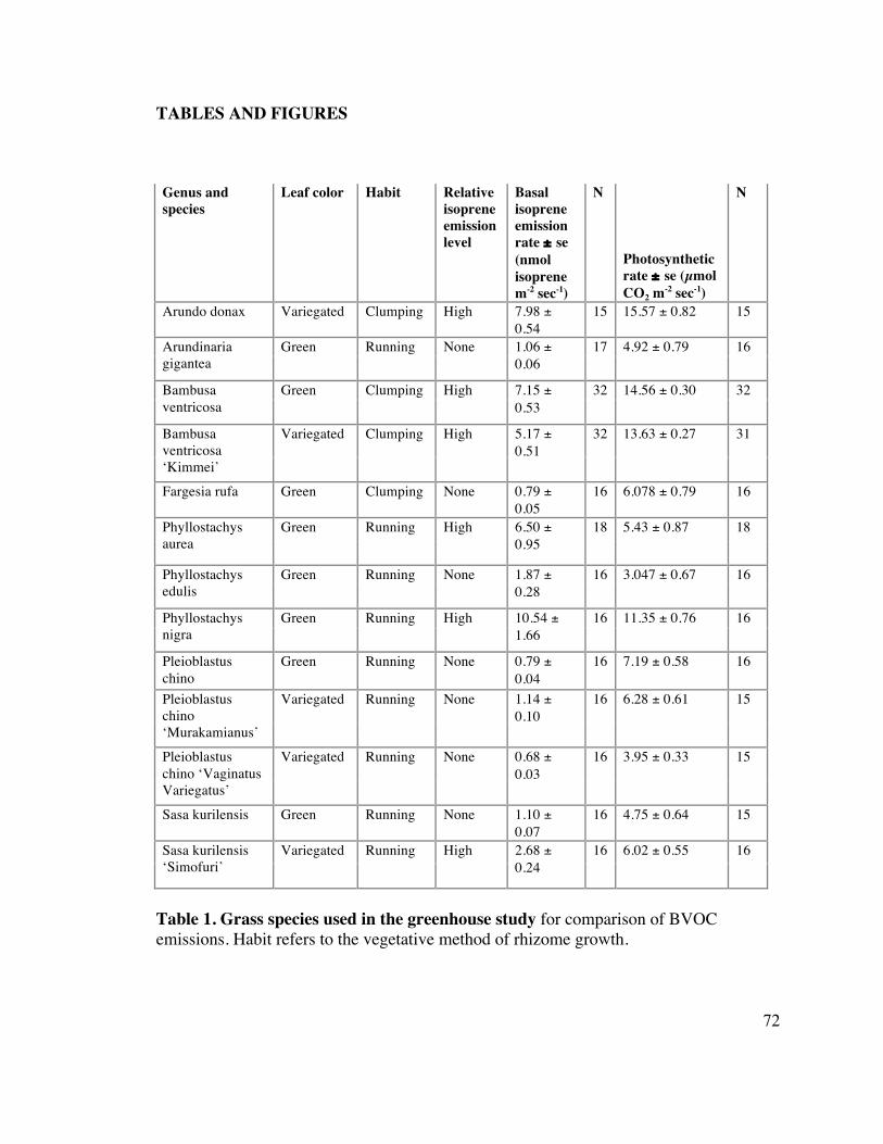
72

TABLES AND FIGURES 1

2 3 Genus and species

Leaf color Habit Relative isoprene emission level

Basal isoprene emission rate ± se (nmol isoprene m-2 sec-1)

N

Photosynthetic rate ± se (µmol CO2 m-2 sec-1)

N

Arundo donax Variegated Clumping High 7.98 ± 0.54

15 15.57 ± 0.82 15

17 4.92 ± 0.79 16 Arundinaria gigantea

Green Running None 1.06 ± 0.06

32 14.56 ± 0.30 32 Bambusa ventricosa

Green Clumping High 7.15 ± 0.53

32 13.63 ± 0.27 31 Bambusa ventricosa ‘Kimmei’

Variegated Clumping High 5.17 ± 0.51

Fargesia rufa Green Clumping None 0.79 ± 0.05

16 6.078 ± 0.79 16

18 5.43 ± 0.87 18 Phyllostachys aurea

Green Running High 6.50 ± 0.95

16 3.047 ± 0.67 16 Phyllostachys edulis

Green Running None 1.87 ± 0.28

16 11.35 ± 0.76 16 Phyllostachys nigra

Green Running High 10.54 ± 1.66

Pleioblastus chino

Green Running None 0.79 ± 0.04

16 7.19 ± 0.58 16

16 6.28 ± 0.61 15 Pleioblastus chino ‘Murakamianus’

Variegated Running None 1.14 ± 0.10

16 3.95 ± 0.33 15 Pleioblastus chino ‘Vaginatus Variegatus’

Variegated Running None 0.68 ± 0.03

Sasa kurilensis Green Running None 1.10 ± 0.07

16 4.75 ± 0.64 15

16 6.02 ± 0.55 16 Sasa kurilensis ‘Simofuri’

Variegated Running High 2.68 ± 0.24

4 Table 1. Grass species used in the greenhouse study for comparison of BVOC 5 emissions. Habit refers to the vegetative method of rhizome growth. 6 7

8

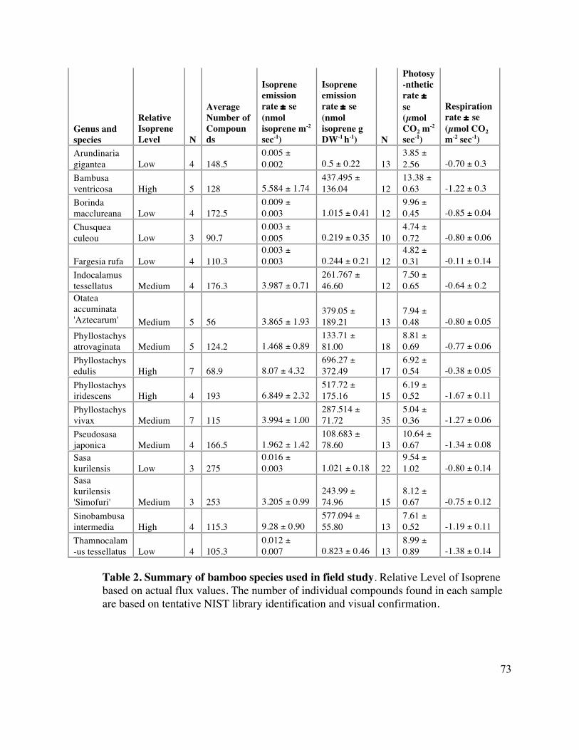
73

1 Table 2. Summary of bamboo species used in field study. Relative Level of Isoprene 2 based on actual flux values. The number of individual compounds found in each sample 3 are based on tentative NIST library identification and visual confirmation. 4

Genus and species

Relative Isoprene Level N

Average Number of Compounds

Isoprene emission rate ± se (nmol isoprene m-2 sec-1)

Isoprene emission rate ± se (nmol isoprene g DW-1 h-1) N

Photosy-nthetic rate ± se (µmol CO2 m-2 sec-1)

Respiration rate ± se (µmol CO2 m-2 sec-1)

Arundinaria gigantea Low 4 148.5

0.005 ± 0.002 0.5 ± 0.22 13

3.85 ± 2.56 -0.70 ± 0.3

Bambusa ventricosa High 5 128 5.584 ± 1.74

437.495 ± 136.04 12

13.38 ± 0.63 -1.22 ± 0.3

Borinda macclureana Low 4 172.5

0.009 ± 0.003 1.015 ± 0.41 12

9.96 ± 0.45 -0.85 ± 0.04

Chusquea culeou Low 3 90.7

0.003 ± 0.005 0.219 ± 0.35 10

4.74 ± 0.72 -0.80 ± 0.06

Fargesia rufa Low 4 110.3 0.003 ± 0.003 0.244 ± 0.21 12

4.82 ± 0.31 -0.11 ± 0.14

Indocalamus tessellatus Medium 4 176.3 3.987 ± 0.71

261.767 ± 46.60 12

7.50 ± 0.65 -0.64 ± 0.2

Otatea accuminata 'Aztecarum' Medium 5 56 3.865 ± 1.93

379.05 ± 189.21 13

7.94 ± 0.48 -0.80 ± 0.05

Phyllostachys atrovaginata Medium 5 124.2 1.468 ± 0.89

133.71 ± 81.00 18

8.81 ± 0.69 -0.77 ± 0.06

Phyllostachys edulis High 7 68.9 8.07 ± 4.32

696.27 ± 372.49 17

6.92 ± 0.54 -0.38 ± 0.05

Phyllostachys iridescens High 4 193 6.849 ± 2.32

517.72 ± 175.16 15

6.19 ± 0.52 -1.67 ± 0.11

Phyllostachys vivax Medium 7 115 3.994 ± 1.00

287.514 ± 71.72 35

5.04 ± 0.36 -1.27 ± 0.06

Pseudosasa japonica Medium 4 166.5 1.962 ± 1.42

108.683 ± 78.60 13

10.64 ± 0.67 -1.34 ± 0.08

Sasa kurilensis Low 3 275

0.016 ± 0.003 1.021 ± 0.18 22

9.54 ± 1.02 -0.80 ± 0.14

Sasa kurilensis 'Simofuri' Medium 3 253 3.205 ± 0.99

243.99 ± 74.96 15

8.12 ± 0.67 -0.75 ± 0.12

Sinobambusa intermedia High 4 115.3 9.28 ± 0.90

577.094 ± 55.80 13

7.61 ± 0.52 -1.19 ± 0.11

Thamnocalam-us tessellatus Low 4 105.3

0.012 ± 0.007 0.823 ± 0.46 13

8.99 ± 0.89 -1.38 ± 0.14

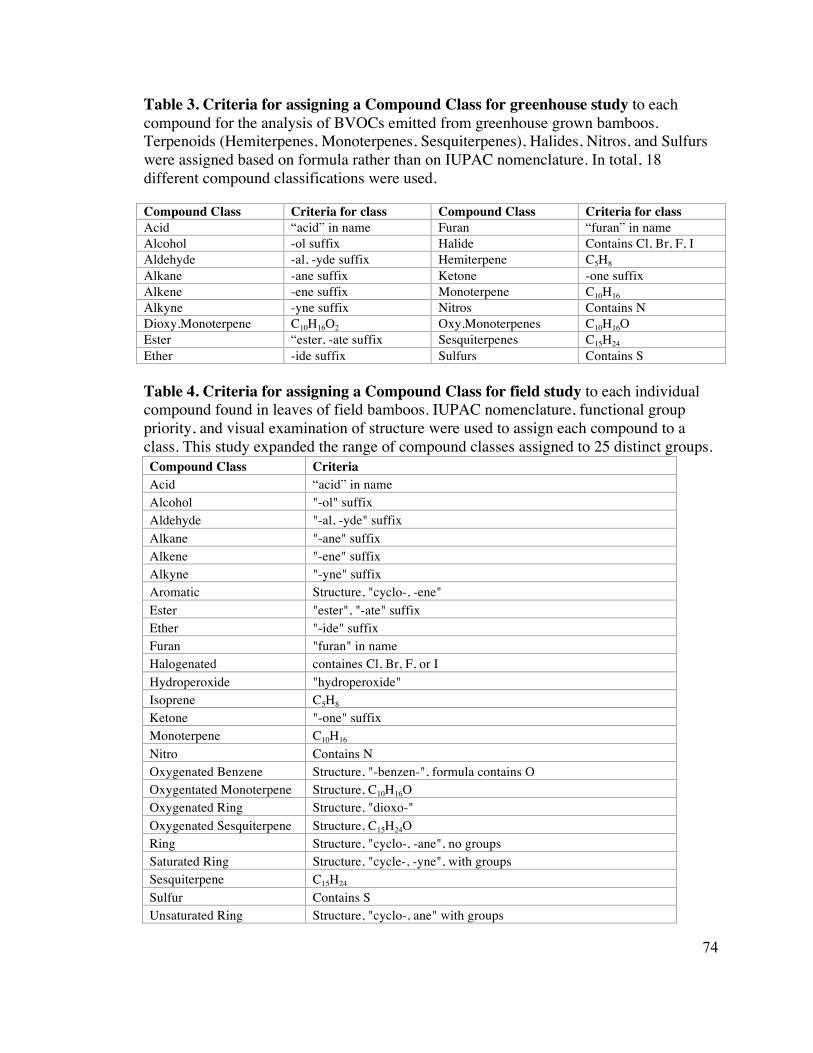
74

Table 3. Criteria for assigning a Compound Class for greenhouse study to each 1 compound for the analysis of BVOCs emitted from greenhouse grown bamboos. 2 Terpenoids (Hemiterpenes, Monoterpenes, Sesquiterpenes), Halides, Nitros, and Sulfurs 3 were assigned based on formula rather than on IUPAC nomenclature. In total, 18 4 different compound classifications were used. 5 6 Compound Class Criteria for class Compound Class Criteria for class Acid “acid” in name Furan “furan” in name Alcohol -ol suffix Halide Contains Cl, Br, F, I Aldehyde -al, -yde suffix Hemiterpene C5H8 Alkane -ane suffix Ketone -one suffix Alkene -ene suffix Monoterpene C10H16 Alkyne -yne suffix Nitros Contains N Dioxy.Monoterpene C10H16O2 Oxy.Monoterpenes C10H16O Ester “ester, -ate suffix Sesquiterpenes C15H24 Ether -ide suffix Sulfurs Contains S 7 Table 4. Criteria for assigning a Compound Class for field study to each individual 8 compound found in leaves of field bamboos. IUPAC nomenclature, functional group 9 priority, and visual examination of structure were used to assign each compound to a 10 class. This study expanded the range of compound classes assigned to 25 distinct groups. 11 Compound Class Criteria Acid “acid” in name Alcohol "-ol" suffix Aldehyde "-al, -yde" suffix Alkane "-ane" suffix Alkene "-ene" suffix Alkyne "-yne" suffix Aromatic Structure, "cyclo-, -ene" Ester "ester", "-ate" suffix Ether "-ide" suffix Furan "furan" in name Halogenated containes Cl, Br, F, or I Hydroperoxide "hydroperoxide" Isoprene C5H8 Ketone "-one" suffix Monoterpene C10H16 Nitro Contains N Oxygenated Benzene Structure, "-benzen-", formula contains O Oxygentated Monoterpene Structure, C10H16O Oxygenated Ring Structure, "dioxo-" Oxygenated Sesquiterpene Structure, C15H24O Ring Structure, "cyclo-, -ane", no groups Saturated Ring Structure, "cycle-, -yne", with groups Sesquiterpene C15H24 Sulfur Contains S Unsaturated Ring Structure, "cyclo-, ane" with groups

12

75

1 2 Figure 1. Phylogeny from Bouchenak-Khelladi et 2008 generated from a Bayesian 3 consensus tree that used combined data sets. The genera selected for our study are 4 circled, with solid lines around genera that were sampled in both the greenhouse and field 5 studies, and dashed lines around genera that were measured in the field study only. 6

7

76

1 Figure 2. Variability in average isoprene flux for 25 genera of bamboo (p<0.0001). 2 N= number of leaf samples run within a given genus. 3

4

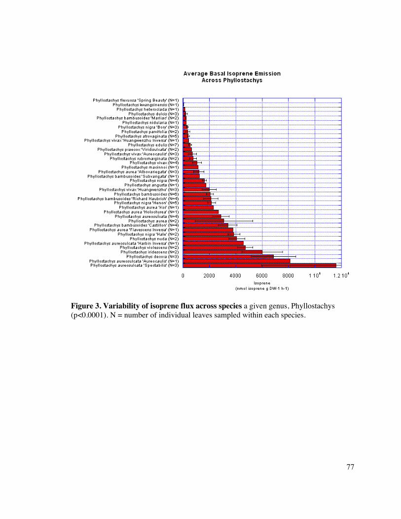
77

1 Figure 3. Variability of isoprene flux across species a given genus, Phyllostachys 2 (p<0.0001). N = number of individual leaves sampled within each species. 3

4

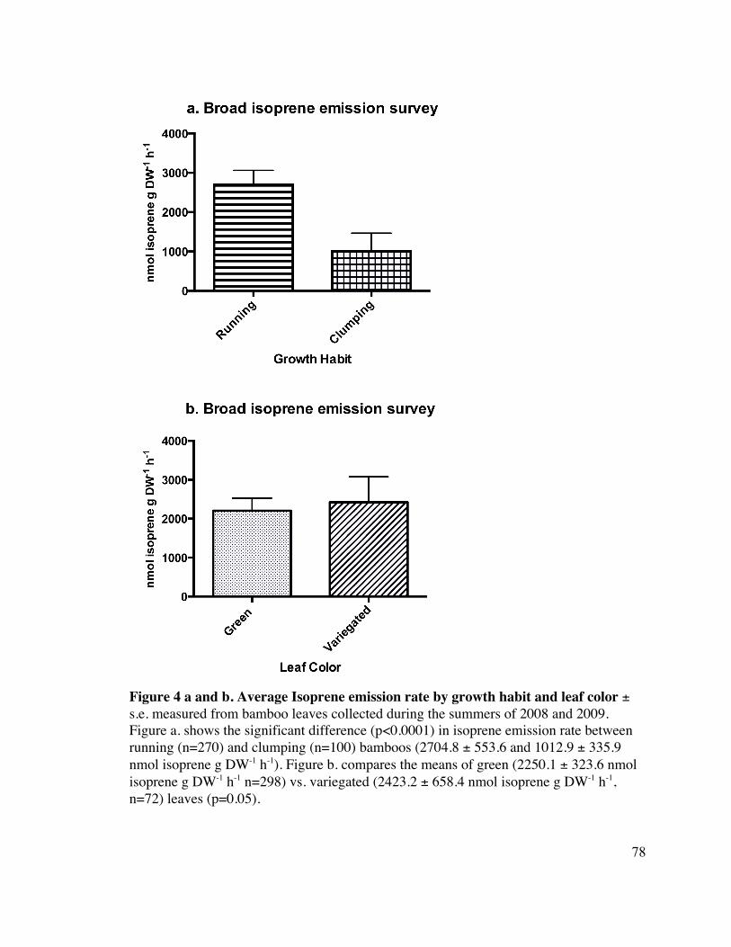
78

1 Figure 4 a and b. Average Isoprene emission rate by growth habit and leaf color ± 2 s.e. measured from bamboo leaves collected during the summers of 2008 and 2009. 3 Figure a. shows the significant difference (p<0.0001) in isoprene emission rate between 4 running (n=270) and clumping (n=100) bamboos (2704.8 ± 553.6 and 1012.9 ± 335.9 5 nmol isoprene g DW-1 h-1). Figure b. compares the means of green (2250.1 ± 323.6 nmol 6 isoprene g DW-1 h-1 n=298) vs. variegated (2423.2 ± 658.4 nmol isoprene g DW-1 h-1, 7 n=72) leaves (p=0.05). 8

9

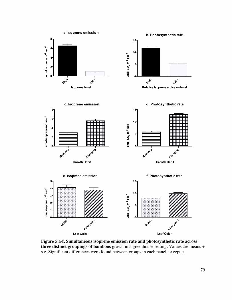
79

1 Figure 5 a-f. Simultaneous isoprene emission rate and photosynthetic rate across 2 three distinct groupings of bamboos grown in a greenhouse setting. Values are means + 3 s.e. Significant differences were found between groups in each panel, except e. 4

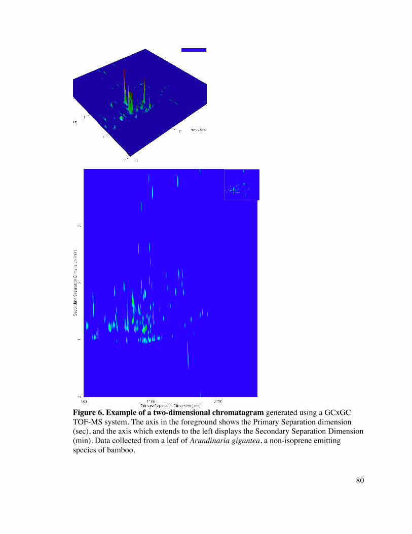
80

1

2 Figure 6. Example of a two-dimensional chromatagram generated using a GCxGC 3 TOF-MS system. The axis in the foreground shows the Primary Separation dimension 4 (sec), and the axis which extends to the left displays the Secondary Separation Dimension 5 (min). Data collected from a leaf of Arundinaria gigantea, a non-isoprene emitting 6 species of bamboo. 7

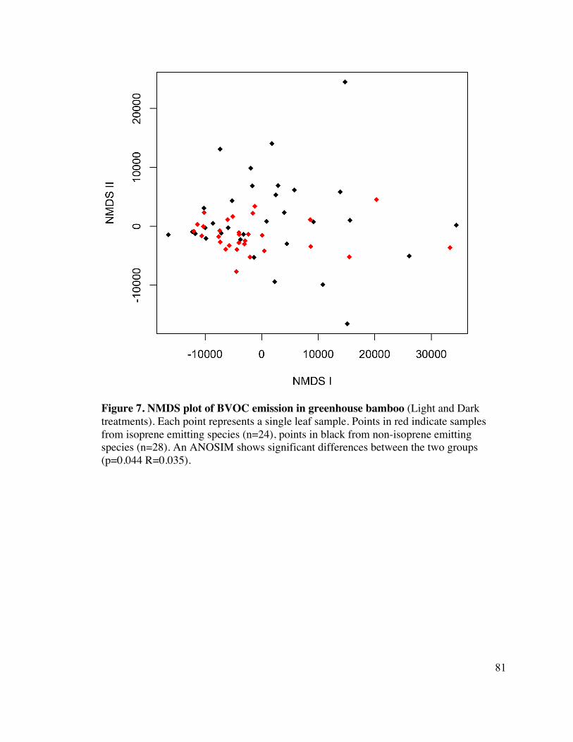
81

1 Figure 7. NMDS plot of BVOC emission in greenhouse bamboo (Light and Dark 2 treatments). Each point represents a single leaf sample. Points in red indicate samples 3 from isoprene emitting species (n=24), points in black from non-isoprene emitting 4 species (n=28). An ANOSIM shows significant differences between the two groups 5 (p=0.044 R=0.035). 6 7

8

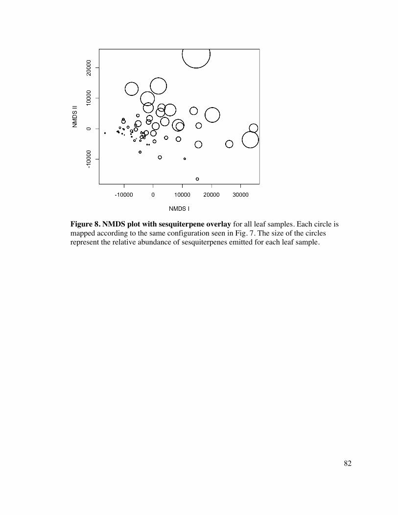
82

1 Figure 8. NMDS plot with sesquiterpene overlay for all leaf samples. Each circle is 2 mapped according to the same configuration seen in Fig. 7. The size of the circles 3 represent the relative abundance of sesquiterpenes emitted for each leaf sample. 4

5

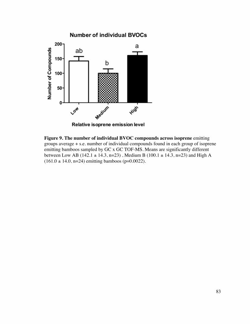
83

1 2 Figure 9. The number of individual BVOC compounds across isoprene emitting 3 groups average + s.e. number of individual compounds found in each group of isoprene 4 emitting bamboos sampled by GC x GC TOF-MS. Means are significantly different 5 between Low AB (142.1 ± 14.3, n=23) , Medium B (100.1 ± 14.3, n=23) and High A 6 (161.0 ± 14.0, n=24) emitting bamboos (p=0.0022). 7

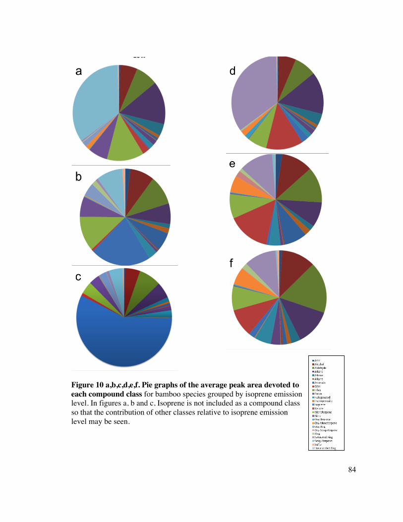
84

2

3

4

5

6

7

8

10 Figure 10 a,b,c,d,e,f. Pie graphs of the average peak area devoted to 12 each compound class for bamboo species grouped by isoprene emission 14 level. In figures a, b and c, Isoprene is not included as a compound class 16 so that the contribution of other classes relative to isoprene emission 18 level may be seen. 20

22

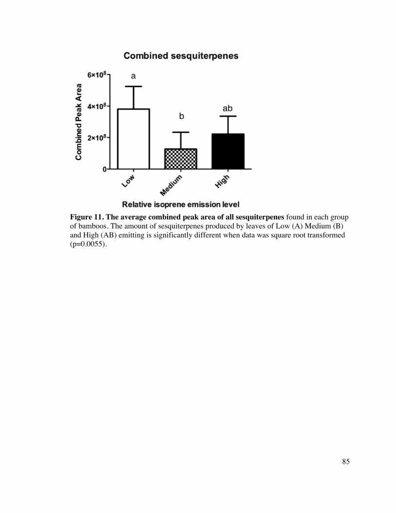
85

1 Figure 11. The average combined peak area of all sesquiterpenes found in each group 2 of bamboos. The amount of sesquiterpenes produced by leaves of Low (A) Medium (B) 3 and High (AB) emitting is significantly different when data was square root transformed 4 (p=0.0055). 5

86

1

2 3 Figure 12. NMDS Ordination of BVOC emission found in field study based on the 4 sum BVOC class peak area m-2 leaf area. Each point is a single leaf sample, coded 5 according to its relative isoprene emission level: High, Medium, or Low. Axis are unit- 6 less and provide a structure to the two-dimensional space. ANOSIM confirms significant 7 differences between each of the three groups (p=0.001, R=0.427). 8 9

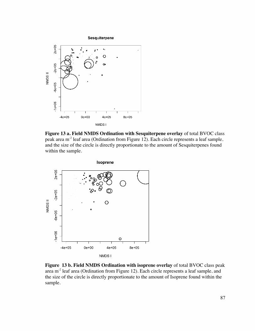
87

1 Figure 13 a. Field NMDS Ordination with Sesquiterpene overlay of total BVOC class 2 peak area m-2 leaf area (Ordination from Figure 12). Each circle represents a leaf sample, 3 and the size of the circle is directly proportionate to the amount of Sesquiterpenes found 4 within the sample. 5

6 Figure 13 b. Field NMDS Ordination with isoprene overlay of total BVOC class peak 7 area m-2 leaf area (Ordination from Figure 12). Each circle represents a leaf sample, and 8 the size of the circle is directly proportionate to the amount of Isoprene found within the 9 sample. 10 11

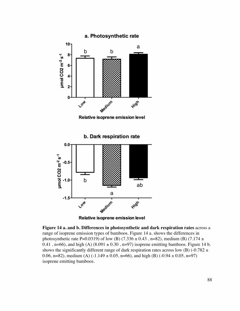
88

1 Figure 14 a. and b. Differences in photosynthetic and dark respiration rates across a 2 range of isoprene emission types of bamboos. Figure 14 a. shows the differences in 3 photosynthetic rate P=0.0319) of low (B) (7.336 ± 0.43 , n=82), medium (B) (7.174 ± 4 0.41 , n=66), and high (A) (8.091 ± 0.30 , n=97) isoprene emitting bamboos. Figure 14 b. 5 shows the significantly different range of dark respiration rates across low (B) (-0.782 ± 6 0.06, n=82), medium (A) (-1.149 ± 0.05, n=66), and high (B) (-0.94 ± 0.05, n=97) 7 isoprene emitting bamboos. 8

9

89

REFERENCES 1

2

Arneth, A. et al “Why Are Estimates of Global Isoprene Emission So Similar.” Atmos. 3

Chem. Phys. 8 (2008): 4605–20. 4

Barta, C, and F Loreto. “The Relationship Between the Methyl-Erythritol Phosphate 5

Pathway Leading to Emission of Volatile Isoprenoids and Abscisic Acid Content in 6

Leaves.” Plant Physiol 141.4 (2006): 1676-83. 7

Bouchenak-Khelladi, Y, N Salamin et al. “Large Multi-Gene Phylogenetic Trees of the 8

Grasses (Poaceae): Progress Towards Complete Tribal and Generic Level 9

Sampling.” Mol Phylogenet Evol 47.2 (2008): 488-505. 10

Calfapietra, C, S Fares, and F Loreto. “Volatile Organic Compounds From Italian 11

Vegetation and Their Interaction With Ozone.” Environ Pollut 157.5 (2009): 1478- 12

86. 13

Calfapietra, C, GS Mugnozza et al. “Isoprene Emission Rates Under Elevated Co2 and 14

O3 in Two Field-Grown Aspen Clones Differing in Their Sensitivity to O3.” New 15

Phytol 179.1 (2008): 55-61. 16

Chapin III, Autumn, Pugnaire. “Evolution of Suites of Traits in Response to 17

Environmental Stress.” The American Naturalist 142 (1993): S78-S92. 18

Cieslik, S, K Omasa, and E Paoletti. “Why and How Terrestrial Plants Exchange Gases 19

With Air.” Plant Biol (Stuttg) 11 Suppl 1 (2009): 24-34. 20

Darbah, JN, TD Sharkey et al. “Differential Response of Aspen and Birch Trees to Heat 21

Stress Under Elevated Carbon Dioxide.” Environ Pollut 158.4 (2010): 1008-14. 22

90

Duhl TR, Helmig D, Guenther A. “Sesquiterpene Emissions From Vegetation: A 1

Review.” Biogeosciences 5 (2008): 761-77. 2

Fares, Silvano, Csengele Barta et al. “Impact of High Ozone on Isoprene Emission, 3

Photosynthesis and Histology of Developing Populus Alba Leaves Directly Or 4

Indirectly Exposed to the Pollutant.” Physiol Plant 128.3 (2006): 456-65. 5

Fortunati, A, C Barta et al. “Isoprene Emission is Not Temperature-Dependent During 6

and After Severe Drought-Stress: A Physiological and Biochemical Analysis.” 7

Plant J 55.4 (2008): 687-97. 8

Geron, C, S Owen et al. “Volatile Organic Compounds From Vegetation in Southern 9

Yunnan Province, China: Emission Rates and Some Potential Regional 10

Implications.” Atmospheric Environment 40.10 (2006): 1759-73. 11

Goldstein, AH, CD Koven et al. “Biogenic Carbon and Anthropogenic Pollutants 12

Combine to Form a Cooling Haze Over the Southeastern United States.” Proc Natl 13

Acad Sci U S A 106.22 (2009): 8835-40. 14

Guenther, A. “Biogenic Hydrocarbon Emissions and Ladcover/Climate Change in a 15

Subtropical Savanna.” Phys. Chem. Earth 24 (1999) 16

Harley, Monson, Lerdau. “Ecological and Evolutionary Aspects of Isoprene Emission 17

From Plants.” Oecologia 118 (1999): 109-23. 18

Holopainen, JK. “Multiple Functions of Inducible Plant Volatiles.” Trends Plant Sci 9.11 19

(2004): 529-33. 20

Kesselmeier, Staudt. “Biogenic Volatile Organic Compounds (Voc): 21

An Overview on Emission, Physiology and Ecology.” Journal of Atmospheric 22

Chemistry 33 (1999): 23-88. 23

91

Kleindienst, Tadeusz E., Mohammed Jaoui et al. “Estimates of the Contributions of 1

Biogenic and Anthropogenic Hydrocarbons to Secondary Organic Aerosol At a 2

Southeastern Us Location.” Atmospheric Environment 41.37 (2007): 8288-300. 3

Klinger, L. F. “Assessment of Volatile Organic Compound Emissions From Ecosystems 4

of China.” J. Geophys. Res. 107.D21 (2002a) 5

Lamb, B, Guenther A Gay, D Westbery H. “A National Inventory of Biogenic 6

Hydrocarbon Emissions.” Atmospheric Environment 21 (1987) 7

Laothawornkitkul, J, JE Taylor et al. “Biogenic Volatile Organic Compounds in the Earth 8

System.” New Phytol 183.1 (2009): 27-51. 9

Lichtenthaler HK, Rohmer M, Schwender J. “Two Independent Biochemical Pathways 10

for Isopentyl Diphosphate and Isoprenoid Biosynthesis in Higher Plants.” 11

Physiologia Plantarum 101 (1997): 643-52. 12

Loreto, F. “On the Monoterpene Emission Under Heat Stress and Increased 13

Thermotolerance of Leaves of Quercus Ilex Fumigated With Selected 14

Monoterpenes.” Plant, Cell and Environment 21 (1998) 15

Loreto, F. “Monoterpene Emission and Monoterpene Synthase Activities in the 16

Mediterranean Evergreen Oak Quercus Ilex L. Grown At Elevated Co2 Concentrations.” 17

Global Change Biology 7 (2001) 18

Loreto, F, and JP Schnitzler. “Abiotic Stresses and Induced Bvocs.” Trends Plant Sci 19

15.3 (2010): 154-66. 20

Maffei, ME, J Gertsch, and G Appendino. “Plant Volatiles: Production, Function and 21

Pharmacology.” Nat Prod Rep 28.8 (2011): 1359-80. 22

92

Monson, RK, RT Jones et al. “Why Only Some Plants Emit Isoprene.” Plant Cell 1

Environ 36.3 (2013): 503-16. 2

Pang, Xiaobing, Yujing Mu et al. “Contribution of Isoprene to Formaldehyde and Ozone 3

Formation Based on Its Oxidation Products Measurement in Beijing, China.” 4

Atmospheric Environment 43.13 (2009): 2142-47. 5

Pankow, J. F., W. Luo et al. “Volatilizable Biogenic Organic Compounds (Vbocs) With 6

Two Dimensional Gas Chromatography-Time of Flight Mass Spectrometry (Gc X 7

Gc-Tofms): Sampling Methods, Vboc Complexity, and Chromatographic Retention 8

Data.” Atmos. Meas. Tech. 5.2 (2012): 345-61. 9

Rasulov, B, K Huve et al. “Evidence That Light, Carbon Dioxide, and Oxygen 10

Dependencies of Leaf Isoprene Emission Are Driven By Energy Status in Hybrid 11

Aspen.” Plant Physiol 151.1 (2009): 448-60. 12

Rosenstiel, T. N., Mark J. Potosnak et al. “Increased Co2 Uncouples Growth From 13

Isoprene Emission in an Agriforest Ecosystem.” Nature 421.6920 (2003): 256-59. 14

Rosenstiel, TN, AL Ebbets et al. “Induction of Poplar Leaf Nitrate Reductase: A Test of 15

Extrachloroplastic Control of Isoprene Emission Rate.” Plant Biol (Stuttg) 6.1 16

(2004): 12-21. 17

Sakulyanontvittaya, Tanarit, Alex Guenther et al. “Secondary Organic Aerosol From 18

Sesquiterpene and Monoterpene Emissions in the United States.” Environ. Sci. 19

Technol. 42.23 (2008): 8784-90. 20

Schnitzler, JP, S Louis et al. “Poplar Volatiles - Biosynthesis, Regulation and 21

(Eco)Physiology of Isoprene and Stress-Induced Isoprenoids.” Plant Biol (Stuttg) 22

12.2 (2010): 302-16. 23

93

Sharkey, TD, AE Wiberley, and AR Donohue. “Isoprene Emission From Plants: Why 1

and How.” Ann Bot 101.1 (2008): 5-18. 2

Staudt, M., and L. Lhoutellier. “Monoterpene and Sesquiterpene Emissions From 3

Quercus Coccifera Exhibit Interacting Responses to Light and Temperature.” 4

Biogeosciences 8.9 (2011): 2757-71. 5

Way, DA, JP Schnitzler et al. “Enhanced Isoprene-Related Tolerance of Heat- and Light- 6

Stressed Photosynthesis At Low, But Not High, Co2 Concentrations.” Oecologia 7

166.1 (2011): 273-82. 8

Wiberley, AE, AR Donohue et al. “Regulation of Isoprene Emission From Poplar Leaves 9

Throughout a Day.” Plant Cell Environ 32.7 (2009): 939-47. 10

11

12

13