Intertemporal Asset Allocation when the

Underlying Factors are unobservable

Chih-Ying Hsiao ∗ Carl Chiarella† Willi Semmler‡

August 8, 2006

Abstract

The aim of this paper is to develop an optimal long-term bond invest-ment strategy which can be applied to real market situations. Thispaper employs Merton’s intertemporal framework to accommodate thefeatures of a stochastic interest rate and the time-varying dynamics ofbond returns. The long-term investors encounter a partial informa-tion problem where they can only observe the market bond prices butnot the driving factors of the variability of the interest rate and thebond return dynamics. With the assumption of Gaussian factor dy-namics, we are able to develop an analytical solution for the optimallong-term investment strategies under the case of full information. Toapply the best theoretical investment strategy to the real market weneed to be aware of the existence of measurement errors representingthe gap between theoretical and empirical models. We estimate themodel based on data for the German securities market and then theestimation results are employed to develop long-term bond investmentstrategies. Because of the presence of measurement errors, we providea simulation study to examine the performance of the best theoreti-cal investment strategy. We find that the measurement errors have agreat impact on the optimality of the investment strategies and thatunder certain circumstance the best theoretical investment strategiesmay not perform so well in a real market situation. In the simulationstudy, we also investigate the role of information about the variabilityof the stochastic interest rate and the bond return dynamics. Our re-sults show that this information can indeed be used to advantage inmaking sensible long-term investment decisions.

∗University of Technology, Sydney, Australia and Bielefeld University, Germany†University of Technology, Sydney, Australia‡New School, New York and Bielefeld University, Germany

1

1 Introduction

The aim of this paper is to construct an optimal long-term strategy for in-vesting in bond securities that would be applicable to trading in real markets.When considering bond investment, there are three reasons why we requirean extension of the well-established Capital Asset Pricing Model (CAPM)of Markowitz (1959), Sharpe (1964), and Lintner (1965) for the conductof bond portfolio management. First, interest rates should be treated asstochastic. One of the main purposes of bond portfolio management is tohedge the risk arising from changing interest rates. Second, the distribu-tions of asset returns should be allowed to vary with time instead of beingonly identically distributed over time as in the CAPM. It is a well-knownfact that the volatility of bond prices decreases as the bonds approach theirmaturity dates. Third, investors who invest in bond assets are usually moreinterested in hedging than speculation. They also tend to adopt some long-term investment plan rather than a simple myopic investment strategy. Inthis paper we will consider the role of the foregoing factors in bond portfo-lio management within the intertemporal framework of Merton (1971,1973,1990).

The now extensive literature in intertemporal asset allocation was initiatedby Merton (1973) who considered the multi-asset model where the asset re-turns are driven by some underlying stochastic factors. His essential insightwas that investors should consider not only a short period mean-variancetrade-off but also a long-term hedging strategy against possible evolutionsof the factor dynamics. Thus, the solution of the optimal intertemporalportfolio problem contains two terms, one the regular (mean-variance) termand the intertemporal hedging term.

In order to apply Merton’s general framework to the practice of the bondportfolio management, the underlying factors need to be specified. In Kimand Omberg (1996), the factor is a Gaussian risk premium. The three factorsin Brennan, Schwartz, and Lagnado (1997) are a short-term interest rate, along-term interest rate and stock dividends. Brennan and Xia (2002) con-sider the real interest rate and the expected inflation rate. Brennan, Wang,and Xia (2004), as well as Munk, Sørensen, and Vinther (2004) concentrateon the interest rate and the Sharpe ratio. Due to the introduction of finan-cial derivatives and the increasing complexity of financial trades, stochasticvolatility is considered in more recent research, for example, in Liu and Pan(2003).

2

Unlike the contributions mentioned above, this paper does not specify theunderlying factors as specific economic variables a priori but estimates themfrom observed bond yields. The solution of the optimal bond portfolio prob-lem relies very much on the dynamic setting for the underlying factors. Forthis reason we let the market data determine the factor dynamics. To thisend we employ the dynamic multidimentional term structure model of Duffieand Kan (1996). The Duffie and Kan model is not only analytically tractablebut also flexible enough to accommodate empirical features, such as level-dependent volatilities, humped and various other shapes for the yield curve.The essential feature of the Duffie-Kan model from our perspective is thelink between the underlying factors and bond yield data. Based on theDuffie-Kan model, we can set up a formula where the underlying factors canbe filtered from market bond yield data.

Before we implement the factor estimation, the identification problem needsto be discussed because of the fact that one data generating process mayhave distinct parameter representations. To solve this problem we needto impose additional conditions on the parameter space so that one datagenerating process has exactly one parameter representation satisfying thegiven identification conditions. This paper will give a different parameterrepresentation from the canonical forms of Dai and Singleton (2000). Ourrepresentation turns out to have an easier solution to the intertemporal assetallocation problem.

To solve the intertemporal asset allocation problem, Merton (1971) pro-posed the method of dynamic programming. Cox, Ingersoll and Ross (1985)(CIR) give analytical solutions for the square root process. In general, how-ever, there are only a few cases that can be solved analytically. Campbelland Viceira (2002) develop an approximate solution for the log-utility case.1

Liu (2005) characterizes the conditions on asset returns that support analyt-ical solutions. In this paper, we apply the Feynman-Kac formula to the HJBequation arising from the method of dynamic programming. The solutionhas an expectation representation, which is similar to the solution obtainedby using the static variational method of Cox and Huang (1989).

In order to give an investment recommendation that can be usefully ap-plied to actual market situations, we estimate the bond pricing model based

1For the log-utility function, the intertemporal effect vanishes.

3

on the yield data of the German securities market. Our empirical task is todecide the most appropriate model in the context of the intertemporal assetallocation problem. Within the framework of this paper, the task reduces tothe determination of the number of the factors in the Gaussian Duffie-Kanmodel.

When fitting the model to market data, the theoretical bond pricing formulacannot hold exactly, but only with some measurement errors. This fact hasimplications for the intertemporal problem since we must take account ofthe fact that the solutions we have obtained are derived from the modelwithout measurement errors. Therefore, we develop a simulation study toinvestigate the impact of the measurement errors on the performance of thebest theoretical investment strategies. In the simulation study, we also con-sider investment strategies based on different information about the bondpricing model. We will assume that some agents know the intertemporalfeature of the bond prices so that they invest according to the intertemporalstrategy, whilst other agents can only observe market bond prices and theyadopt an investment strategy based on a risk-return trade-off.

The remainder of the paper is organized as follows. Section 2 sets up themodel for the intertemporal asset allocation problem. The first part of Sec-tion 2 reviews the Duffie-Kan multifactor term structure model and discussesthe model identification problem. The second part develops the optimal in-tertemporal asset allocation strategy based on the Duffie-Kan model. Theform of the solution of the intertemporal problem obtained by using theFeynman-Kac formula is provided. Section 3 presents the empirical study ofthe bond pricing model where we estimate the Gaussian Duffie-Kan modelbased on the data for the German securities market. The simulation studyis provided in Section 4. The last section draws some conclusions. A numberof technical results are gathered in the appendices.

2 The Intertemporal Asset Allocation Problem

In this section we set up the model for the intertemporal decision problem.The intertemporal asset allocation problem is to choose optimal asset allo-cation strategies in order to maximize agents’ long-term expected utility ofconsumption. The form of the optimal asset allocation strategies dependson the kinds of assets available for investment. We consider an investmentopportunity set that only consists of bond assets, and use the Duffie and Kan(1996) framework to model them. The Duffie and Kan model is reviewed

4

in Section 2.1. Section 2.2 reviews the method of dynamic programmingproposed by Merton (1971), which we use to solve the intertemporal as-set allocation problem, and solves the optimal asset allocation strategies byemploying the Feynman-Kac formula.

2.1 Modelling Bond Assets

First, we review the Duffie-Kan affine family briefly and then discuss theidentification problem for this family.

2.1.1 The Duffie-Kan affine family

The Duffie-Kan affine family of bond models has the characteristics that thebond price P (t, T , Xt) is given by the exponential affine form

P (t, T , Xt) = e−A(T−t)−B(T−t)�Xt , (1)

where t is the current time and T is the maturity date. The bond pricedepends on the current level of the factors Xt. The factors Xt are repre-sented by an n-dimensional stochastic process that will be specified later.All bonds considered in this paper pay no coupons. The coefficients A(τ)and B(τ)� = (B1(τ), · · · , Bn(τ)) are differentiable functions. The bondpayout at the maturity is set to be 1, so that P (T , T , XT ) = 1. This condi-tion in turn implies that the initial conditions for the coefficients are givenby A(0) = Bi(0) = 0, for all i = 1, · · · , n.

The bond yield y(t, T , Xt) is defined as an average return, so it has theaffine structure

y(t, T , Xt) :=lnP (T , T , XT ) − lnP (t, T , Xt)

T − t=

A(T − t)T − t

+B(T − t)�

T − tXt .

(2)The spot interest rate Rt is defined as the instantaneous yield, which canbe represented by

Rt = lims↑t

y(Xs, t − s) = ξ0 + ξ�1 Xt , (3)

where we let ξ0 = A′(0) and ξ1 = B′(0).

Duffie and Kan (1996) show that the exponential affine bond price (1) issupported by affine dynamics for the underlying factors

dXt = K(θ − Xt)dt + Γ√

StdWt , (4)

5

where θ is an n × 1 constant vector, K and Γ = (γij)i,j=1,··· ,n are n × nconstant matrices, and St is a diagonal n × n matrix with affine elementsSi(Xt) = αi + β�

i Xt. The noise term is represented by a standard (orthog-onal) n-dimensional Wiener process Wt .

2.1.2 A subfamily: The Gaussian factor model

In this paper we only consider a subfamily of the Duffie-Kan family, namelythe one where the factor Xt follows an n-dimensional Gaussian process

dXt = K(θ − Xt)dt + ΓdWt . (5)

We require further that the matrix K be positive definite so that the processXt is stationary. Also, the matrix K is required to have distinct eigenvalues.The volatility coefficient matrix Γ is assumed to be full-rank so that any fac-tor noise ΓidWt, where Γi denotes the i-th row in Γ, cannot be substitutedby any linear combination of the other factor noises.

Applying Ito’s Lemma to the bond price (1), the dynamics of the instanta-neous bond return are given by

dP (t, T , Xt)P (t, T , Xt)

= μP (T − t, Xt)dt − B(T − t)�ΓdWt , (6)

where

μP (τ, Xt) = A′(τ) + B′(τ)�Xt −B(τ)�K(θ−Xt) +12

n∑i,j=1

Bi(τ)Bj(τ)ΓiΓ�j .

(7)

The bond market satisfies the standard no-arbitrage condition

μP (τ, Xt) − Rt = −B(τ)�Γλ , (8)

for all τ > 0, where λ is an n × 1 constant vector λ = (λ1, · · · , λn). Eachλi can be interpreted as the market price of the factor innovation Wit. Theno-arbitrage condition (8) states that the excess return over the riskless re-turn on the left hand side should be equal to the risk premia on the righthand side.

6

The no-arbitrage condition (8) requires that the coefficients A(τ) and B(τ)satisfy the ordinary differential equations

B′(τ) = −K�B(τ) + ξ1 , (9)

A′(τ) = (Kθ − Γλ)�B(τ) − 12

n∑i,j=1

Bi(τ)Bj(τ)ΓiΓ�j + ξ0 . (10)

2.1.3 The model identification problem

When considering a multifactor term structure model such as the one givenby equations (1), (5), (9) and (10), we are inevitably confronted with anidentification problem, especially when we do not specify the factors Xt asspecific economic variables but rather seek to infer them from market data.The identification problem arises due to the fact that different parameterrepresentations in the multifactor term structure model can generate thesame bond prices. This can be illustrated as follows. To a set of factorsXt in the bond pricing formula (1), we can apply a full-rank transformationL and we still get the same multifactor term structure model based on thetransformed factors XL

t := LXt since

y(t, t + τ, Xt) =A(τ)

τ+

B(τ)�

τXt =

A(τ)τ

+(L−1�B(τ))�

τXL

t .

The transformed factors XLt follow the stochastic differential equation

dXLt = LdXt = LKL−1(Lθ − XL

t )dt + LΓdWt ,

which is different from the original factor dynamics (5).

To solve the identification problem, we need to impose additional conditionson the parameters (θ,K, Γ, λ, ξ0, ξ1) such that for any bond yield expressionof the form (2) there exists only one parameter representation satisfyingthose conditions.

Property 1 Consider the bond yield model (2), where the factors Xt followthe dynamics (5) and the coefficients B(τ) and A(τ) satisfy the no-arbitrageconditions (9) and (10). Assume that the parameters (θ,K, Γ, λ, ξ0, ξ1) ofthis model satisfy the identification conditions:

7

(i) K in (5) is diagonal,

(ii) θ in (5) is equal to (0, · · · , 0)�,

(iii) ξ1 in (9) is equal to(1, · · · , 1

)�,

(iv) Γ in (5) is lower-triangular.

Then, for each data generating process (2) for y(t, t + τ, Xt), there existsonly one corresponding parameter representation (up to permutations of thefactors Xt).

Our parameter representation given in Property 1 is different from thecanonical representation of Dai and Singleton (2000, p.1948) where, in ournotation, the matrix K is lower-triangular while Γ is diagonal. In our repre-sentation, each factor Xi has a distinct mean-reverting speed represented bythe parameter κi while in the Dai and Singleton representation, the factorsare stochastic processes independent of each other. These two representa-tions are equivalent in the sense that we can find a full-rank linear matrixto transform one representation to the other and vice verse. The reasonwhy we choose this parameter representation rather than the canonical rep-resentation is because of its convenience in solving for the coefficient B(τ)in equation (9) and the intertemporal optimal strategies that will be intro-duced later.

The following property solves the coefficients Bi(τ), A(τ) in the bond priceformula (1) satisfying the identification conditions given in Property 1.

Property 2 Let κ1, · · · , κn be the elements on the diagonal of K. Then,the coefficients B(τ) and A(τ) satisfying the no-arbitrage conditions (9) and(10) with the parameter restrictions given in Property 1 are solved as

Bi(τ) =1κi

(1 − eκiτ ) , ∀i = 1, · · · , n (11)

A(τ)τ

=n∑

i=1

Γiλ

κi

(− 1 +1 − e−κiτ

κiτ

)+ ξ0 (12)

−12

n∑i,j=1

ΓiΓ�j

κiκj

(1 − 1 − e−κiτ

κiτ− 1 − e−κjτ

κjτ+

1 − e−(κi+κj)τ

(κi + κj)τ)

,

where B(τ) =(B1(τ), · · ·Bn(τ)

)�.

8

2.2 Optimal Asset Allocation Strategies

2.2.1 The intertemporal model

The intertemporal asset allocation problem considers homogenous agentswhose utility is represented by the CRRA (Constant Relative Risk Aversion)utility function

U(C) =C1−γ

1 − γ, (13)

where γ > 0 and γ �= 1. Initially the agents have endowment V0 where Vt

represents wealth at time t. The objective of these agents is to maximizethe expected future utility

E0

[e−δT U(VT )

]. (14)

The agents maximize their objective (14) by choosing an investment plan(α1t, · · · , αnt) for each moment t ∈ [0, T ]. Each αit represents the invest-ment proportion in the i-th bond relative to the total wealth level.

For the multifactor no-arbitrage bond model introduced above, we canchoose n bonds with distinct maturity dates T 1, · · · , Tn, as many as thenumber of the factors, to span all bond returns, see, for example, Chiarella(2004). In other words, any bond can be replicated by a portfolio consistingof these n chosen bonds.

Let Pit := P (t, T i, Xt) denote the price of the i-th bond maturing at timeT i. From (6), the bond return dynamics can be represented in the vectorform ⎛

⎜⎝dP1tdP1t...

dPntPnt

⎞⎟⎠ = μtdt + ΣtdWt ,

where

μt :=

⎛⎜⎝μP (T 1 − t, Xt)

...μP (Tn − t, Xt)

⎞⎟⎠ (15)

Σt := −BtΓ , with Bt :=

⎛⎜⎝B1(T 1 − t) · · · Bn(T 1 − t)

.... . .

...B1(Tn − t) · · · Bn(Tn − t)

⎞⎟⎠ . (16)

9

Then, the evolution of wealth due to the the investment plan (α0t, · · · , αnt)can be represented by2

dVt

Vt= Rtdt + α�

t

((μt − Rt1)dt − BtΓdWt

), (17)

where α�t := (α1t, · · · , αnt), and 1 := (1, · · · , 1)�.

The remaining investment proportion α0t := 1 −∑ni=1 αit, which can be

positive or negative, represents the investment position in the money mar-ket which earns the riskless return Rt.

2.2.2 The solution via dynamic programming

Let J(t, T, Vt, Xt) be the value function, which is defined as the maximizedobjective function (14) for the sub-period [t, T ], so that

J(t, T, Vt, Xt) = maxαs;t≤s≤T

{Et

[e−δT U(VT )

]}. (18)

The value function depends on the wealth Vt and the level of the underlyingfactor Xt at the initial time of the sub-period. The Hamilton-Jacobi-Bellman(HJB) equation3 characterizes the first order condition that yields the opti-mal decisions and is given by

0 = maxαt

{∂

∂tJ +

(Rt + α�

t (μt − Rt1))JV Vt

+12α�

t ΣtΣ�t αtJV V V 2

t + (θ − Xt)�K�JX (19)

+α�t ΣtΓ�JV XVt +

12

n∑i,j=1

ΓiΓ�j JXi,Xj

}.

We observe that during the time period s ∈ [t, T ] the factor dynamics forXs, given in (5), are independent of the wealth level Vs. Furthermore,the percentage wealth change dVs/Vs, defined by (17), is also independentof the wealth level Vs. Given the just-stated independence of Vt, it turnsout that the initial wealth level Vt does not affect the optimal decisions α∗

s

2See Merton (1971) .3The HJB equation states that the optimal lifetime utility over [t, T ] should be equal to

the optimal momentum utility for a short time interval [t, t+ dt) plus the optimal lifetimeutility over [t+dt, T ]. See Kamien and Schwartz (1991: 264-271) for a heuristic discussionand Chapter 11 in Øksendal(2000) for a rigorous derivation.

10

over the period s ∈ [t, T ], and it can be treated as a scalar multiplier ofthe intertemporal optimization problem (18). So, we can rewrite the valuefunction as

J(t, T, Vt, Xt)

= maxαs;t≤s≤T

{V 1−γ

t e−δTEt[U(VT

Vt)]}

= V 1−γt J(t, T, 1, Xt) = e−δtU(Vt)Φ(t, T, Xt)γ , (20)

where we setΦ(t, T, Xt)γ := eδt(1 − γ)J(t, T, Xt, 1) .

The product form (20) separates Vt from the other dependent variables.

Using the product form (20), the HJB equation (19) may be written as4

0 = maxαt

{−δJ + (1 − γ)

(Rt + α�

t (μt − Rt1))J

−12(1 − γ)(−γ)α�

t ΣtΣ�t αtJ + γ(θ − Xt)�K�ΦXi

ΦJ

+(1 − γ)γα�t ΣtΓ�ΦXi

ΦJ

+12

n∑i,j=1

ΓiΓ�j

(γ(γ − 1)

ΦXi

ΦΦXj

Φ+ γ

ΦXiXj

Φ

)J

},

from which the first order condition (FOC) for αt leads to the expressionfor the optimal αt given by

α∗t =

1γ

(ΣtΣ�t )−1(μt − Rt1)︸ ︷︷ ︸

Mean-Variance Efficient

+ (ΣtΣ�t )−1ΣtΓ�ΦX

Φ︸ ︷︷ ︸Intertemporal Hedging

. (21)

The first term in the solution of the optimal portfolio (21) is the mean-variance efficient portfolio, where the agents’ portfolio decisions are based

4We abbreviate J(t, T, Xt) to J , and use the following equalities

∂

∂tJt = −δJ + γ(

∂

∂tΦ)

1

ΦJ , JX = γ

ΦX

ΦJ ,

JV V = (1 − γ)J , JV V V 2 = (1 − γ)(−γ)J ,

JV XV = (1 − γ)γΦXi

ΦJ , JXi,Xj =

“γ(γ − 1)

ΦXi

Φ

ΦXj

Φ+ γ

ΦXiXj

Φ

”J .

11

on the return-risk trade-off. The second term arises only in an intertempo-ral framework and is due to the variation of the factors represented by thevolatility coefficient Γ in the factor dynamics (5). In a static framework, Γis equal to zero, then this term vanishes. This decomposition of the opti-mal intertemporal portfolio decision is one of the profound contributions ofMerton (1971,1973).

Applying the equation (21) to the HJB equation (19), the HJB equationcan be transformed into the partial differential equation

0 =∂

∂tΦ +

(K(θ − Xt) +

1 − γ

γΓΣ−1

t (μt − Rt1))�

ΦX

+12

n∑i,j=1

ΦXiXjΓiΓ�j (22)

+Φ(− δ

γ+

1 − γ

γRt +

1 − γ

2γ2(μt − Rt1)�(ΣtΣ�

t )−1(μt − Rt1))

.

For the finite time case we let the final utility function be equal to thetemporary utility function

J(T, T, VT , XT ) = U(VT ) .

Thus, the boundary condition for the multiplicative part Φ(t, T, Xt) is

Φ(T, T, XT ) = 1 , (23)

due to the definition of Φ in equation (20).

So, the problem of intertemporal asset allocation now reduces to the prob-lem of solving the nonlinear second order partial differential equation (22)for Φ.

2.2.3 Solving the HJB equation via the Feymann-Kac formula

To simplify the HJB equation (22), we let

ht := − δ

γ+

1 − γ

γRt +

1 − γ

2γ2λ�λ . (24)

Together with the fact that

Σ−1t (μt − Rt) = λ ,

12

which is based on the no-arbitrage condition (8), the HJB equation can berewritten further as

0 =∂

∂tΦ +

(K(θ − Xt) + Γ

1 − γ

γλ)�

ΦX +12

n∑i,j=1

ΦXiXjΓiΓ�j + Φht . (25)

The application of the the Feymann-Kac formula5 to represent the solutionis straightforward and involves associating the HJB equation (25) with thepartial differential equation (59) in the Appendix.

We provide the solution here and the proof is given in Section 6.1 of theappendix.

Property 3 The solution Φ(t, T, Xt) for the partial differential equation(25) with the boundary condition (23) is given by the expectation operatorrepresentation

Φ(t, T, Xt) = Et,Xt

[e

R Tt h(Xs,s)ds dPT

dPT

], (26)

where the Radom-Nikodym derivative appearing in (26) is given by

dPT

dPT= exp

(1 − γ

γλ�(WT − Wt) − (1 − γ)2

2γ2λ�λ(T − t)

), (27)

and Et,Xt is the expectation operator with respect to the process Xs, t ≤ s ≤T , satisfying (5) with initial value Xt.

The reader may note that the expectation operator expression (26) is verysimilar to the martingale solution obtained by the static variational methodof Cox and Huang (1989). It can be shown that the expectation operatorrepresentation (26) is equivalent to the solution of Cox and Huang (1989)in Hsiao (2006). Here we provide another way to obtain the martingalesolution.

3 Estimating the Factors based on Market Data

In this section we estimate the parameters and the unobservable stochasticfactors in the bond pricing formula (2) based on actual market data. Thecoefficients A(τ) and B(τ) in (2) are given in equations (12) and (11) and

5See Theorem 1 in Section 6.2 of the Appendix.

13

the factor Xt follows the dynamics (5). We will determine parameter values(K, Γ, λ, ξ0

)in order to fit the observed bond yield data y(t, T , Xt). The

parameter values are determined by the maximum likelihood method.

The bond yield data are obtained from the Homepage of Deutsche Bun-desbank (German Federal Bank)6. The yield data are derived from theinterest rates on Federal securities using the method of Nelson and Siegel7.The bond yields used here are medium- and long-term ones with time tomaturity of 1 year, 3, 5, 8, and 10 years8 corresponding to our purpose forconstructing long-term asset allocation strategies. We have chosen the timehorizon January 03, 2003 to February 10, 2005 because the bonds were ac-tively traded in this period. All data are available on a daily basis, so thereare 535 observation points. Figure 1 plots the data and their descriptivestatistics are given in Table 1.

Year2003 2004 2005

1%

2%

3%

4%

5%

1 Year Yield

3 Year Yield

5 Year Yield

Figure 1: German Yield Curve6The data source is located at “http://www.bundesbank.de/statistik/statistik.en.php”,

then click “Time Series Database”, then “Interest Rates”, then “capital market”, then“Term structure of interest rates in the debt securities market - estimated values”, then“Yields, derived from the term structure of interest rates, on listed Federal securities withannual coupon payments (monthly and daily data)”.

7See the Monthly Report of the Deutsche Bundesbank, October 1997: 61-66.8Those time series that are labelled by wt3211, wt3215, wt3219, wt3225, and wt3229

respectively.

14

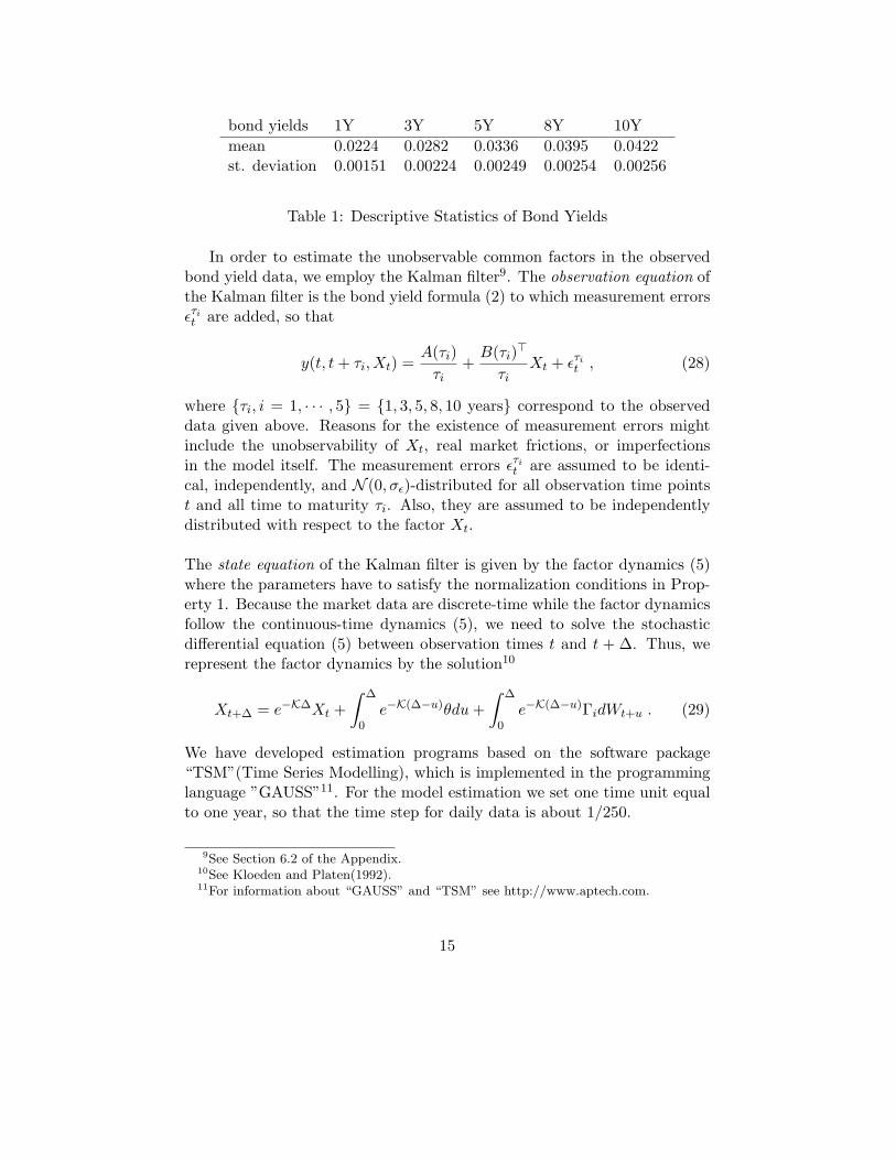
bond yields 1Y 3Y 5Y 8Y 10Ymean 0.0224 0.0282 0.0336 0.0395 0.0422st. deviation 0.00151 0.00224 0.00249 0.00254 0.00256

Table 1: Descriptive Statistics of Bond Yields

In order to estimate the unobservable common factors in the observedbond yield data, we employ the Kalman filter9. The observation equation ofthe Kalman filter is the bond yield formula (2) to which measurement errorsετit are added, so that

y(t, t + τi, Xt) =A(τi)

τi+

B(τi)�

τiXt + ετi

t , (28)

where {τi, i = 1, · · · , 5} = {1, 3, 5, 8, 10 years} correspond to the observeddata given above. Reasons for the existence of measurement errors mightinclude the unobservability of Xt, real market frictions, or imperfectionsin the model itself. The measurement errors ετi

t are assumed to be identi-cal, independently, and N (0, σε)-distributed for all observation time pointst and all time to maturity τi. Also, they are assumed to be independentlydistributed with respect to the factor Xt.

The state equation of the Kalman filter is given by the factor dynamics (5)where the parameters have to satisfy the normalization conditions in Prop-erty 1. Because the market data are discrete-time while the factor dynamicsfollow the continuous-time dynamics (5), we need to solve the stochasticdifferential equation (5) between observation times t and t + Δ. Thus, werepresent the factor dynamics by the solution10

Xt+Δ = e−KΔXt +∫ Δ

0e−K(Δ−u)θdu +

∫ Δ

0e−K(Δ−u)ΓidWt+u . (29)

We have developed estimation programs based on the software package“TSM”(Time Series Modelling), which is implemented in the programminglanguage ”GAUSS”11. For the model estimation we set one time unit equalto one year, so that the time step for daily data is about 1/250.

9See Section 6.2 of the Appendix.10See Kloeden and Platen(1992).11For information about “GAUSS” and “TSM” see http://www.aptech.com.

15

In order to determine how many common factors Xt should be chosen forthe underlying dynamics for the bond yields, we implement the model esti-mation for one-, two-, and three-dimensional factors Xt and then choose thebest model according to information criteria, namely, the Akaike, Bayesianand Hannan-Quinn information criteria.

At a maximum, the gradient of the log-likelihood is equal to zero. In thenumerical implementation, the convergence tolerance for the gradient is setto be 10−5. However, with this setting, we were not able to obtain conver-gence for the three-dimensional factor model so we relaxed the convergencetolerance to 0.07 in order to obtain a set of parameter estimates.

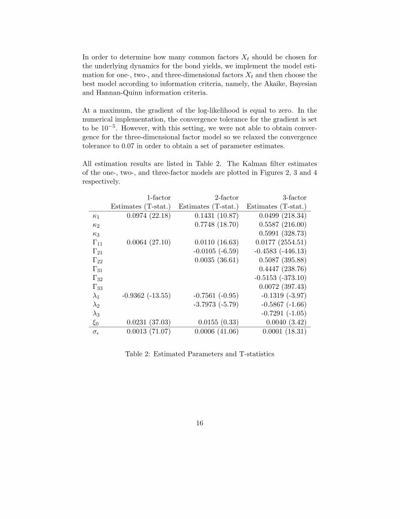
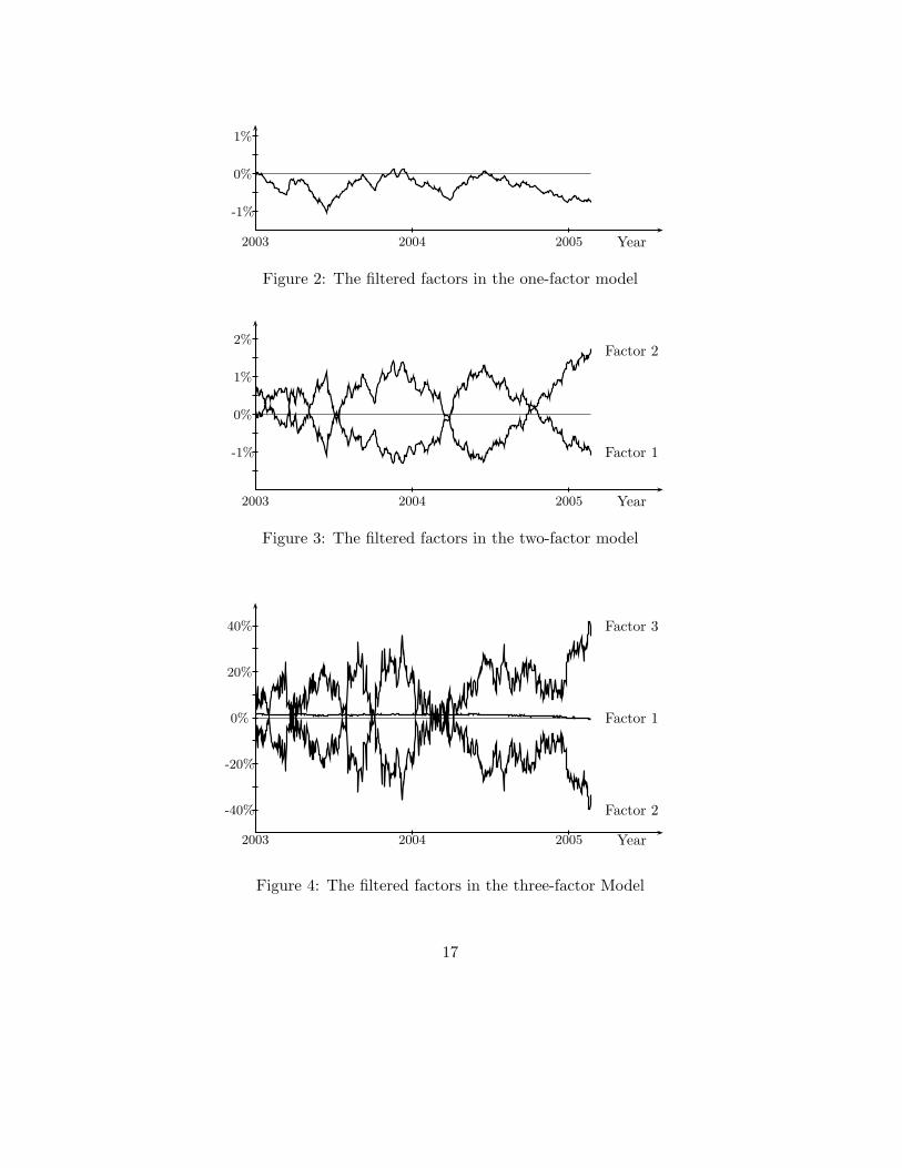
All estimation results are listed in Table 2. The Kalman filter estimatesof the one-, two-, and three-factor models are plotted in Figures 2, 3 and 4respectively.

1-factor 2-factor 3-factorEstimates (T-stat.) Estimates (T-stat.) Estimates (T-stat.)

κ1 0.0974 (22.18) 0.1431 (10.87) 0.0499 (218.34)κ2 0.7748 (18.70) 0.5587 (216.00)κ3 0.5991 (328.73)Γ11 0.0064 (27.10) 0.0110 (16.63) 0.0177 (2554.51)Γ21 -0.0105 (-6.59) -0.4583 (-446.13)Γ22 0.0035 (36.61) 0.5087 (395.88)Γ31 0.4447 (238.76)Γ32 -0.5153 (-373.10)Γ33 0.0072 (397.43)λ1 -0.9362 (-13.55) -0.7561 (-0.95) -0.1319 (-3.97)λ2 -3.7973 (-5.79) -0.5867 (-1.66)λ3 -0.7291 (-1.05)ξ0 0.0231 (37.03) 0.0155 (0.33) 0.0040 (3.42)σε 0.0013 (71.07) 0.0006 (41.06) 0.0001 (18.31)

Table 2: Estimated Parameters and T-statistics

16

Year2003 2004 2005

-1%

0%

1%

Figure 2: The filtered factors in the one-factor model

Year2003 2004 2005

-1%

0%

1%

2%

Factor 1

Factor 2

Figure 3: The filtered factors in the two-factor model

Year2003 2004 2005

-40%

-20%

0%

20%

40%

Factor 1

Factor 2

Factor 3

Figure 4: The filtered factors in the three-factor Model

17

With regard to the estimates we make a number of observations. First, allmean-reverting parameters κi are quite small for all three models. Second,the two innovations in the two-factor model, which are represented by thenoise terms Γ11W1t and Γ21W1t +Γ22W2t, are highly (negatively) correlatedwith the correlation coefficient −0.9485 based on the estimation values inTable 2. This high correlation of the factor innovations leads to high correla-tion of the factors processes X1t, X2t, as shown in Figure 3. Third, a similarhigh correlation can be also found between the second and the third factorinnovations in the three-factor model, which are represented by the noiseterms

∑2i=1 Γ2iWit and

∑3i=1 Γ3iWit. The correlation coefficient is equal to

−0.9997. The estimated factors are displayed in Figure 4. In the three-factorestimation we also observe that the estimated second and third factors varyover an abnormally large scale compared with the observed market yields.

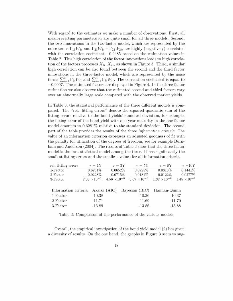
In Table 3, the statistical performance of the three different models is com-pared. The “rel. fitting errors” denote the squared quadratic sum of thefitting errors relative to the bond yields’ standard deviation, for example,the fitting error of the bond yield with one year maturity in the one-factormodel amounts to 0.6281% relative to the standard deviation. The secondpart of the table provides the results of the three information criteria. Thevalue of an information criterion expresses an adjusted goodness of fit withthe penalty for utilization of the degrees of freedom, see for example Burn-ham and Anderson (2004). The results of Table 3 show that the three-factormodel is the best statistical model among the three. It has significantly thesmallest fitting errors and the smallest values for all information criteria.

rel. fitting errors τ = 1Y τ = 3Y τ = 5Y τ = 8Y τ =10Y1-Factor 0.6281% 0.0652% 0.0725% 0.0813% 0.1441%2-Factor 0.0228% 0.0715% 0.0181% 0.0122% 0.0277%3-Factor 2.03 ×10−6 4.56 ×10−6 3.67 ×10−6 1.32 ×10−6 1.45 ×10−6

Information criteria Akaike (AIC) Bayesian (BIC) Hannan-Quinn1-Factor -10.38 -10.36 -10.372-Factor -11.71 -11.69 -11.703-Factor -13.89 -13.86 -13.88

Table 3: Comparison of the performance of the various models

Overall, the empirical investigation of the bond yield model (2) has givena diversity of results. On the one hand, the graphs in Figure 3 seem to sug-

18

gest that the second factor is redundant because the trajectories of the twofactors are almost like a mirror image of each other. The estimated factortrajectories in the three-factor model fluctuate on a wide scale that is muchlarger then that of the bond yields themselves. On the other hand, from thestatistical point of view, however, it seems that the more factors, the betterthe statistical performance among the three models.

The estimated models will be used in Section 4 for the simulation studyof portfolio performance. We discard the the three-factor model because ofits wild behavior, which might lead to extreme investment strategies. Weemploy the estimation results of the one- and two-factor models.

4 Optimal Portfolios and Simulation Study

In this section we give explicit forms for the optimal intertemporal portfoliostrategies. We then undertake a simulation study of portfolio performancebased on the estimation results of Section 3.

Given the solution of the value function in Section 2.2.3, we give explictforms of the optimal intertemporal portfolio strategies in Section 4.1. Thoseoptimal strategies, however, are constructed without measurement errors inthe pricing formula (28). In order to apply these optimal strategies to realmarket situations, we need to take account of the existence of the measure-ment errors in the pricing formulas. Then, the following questions arisesnaturally. Do the best theoretical (intertemporal) investment strategy stillperform well in the presence of the measurement errors? How do the mea-surement errors affect performance of the strategies? In Section 4.2 we willprovide a simulation study that seeks to answer these questions. In the sim-ulation study we are also interested in the problem of partial information,when investors do not have an intertemporal model for investment planningbut rather follow the conventional strategy of choosing the mean-varianceefficient (MVE) portfolios. We will compare the MVE strategies with theintertemporal optimal strategies.

4.1 Optimal Portfolio without Measurement Errors

Property 4 The explicit solution of Φ(t, T, x) satisfying the expectation op-erator representation (26) where the parameters

(K, Γ, λ, ξ0

)satisfy the iden-

19

tification conditions given in Property 1, is given by

Φ(t, T, Xt) = f(t, T )e1−γ

γB(T−t)Xt , (30)

where

ln f(t, T ) = − δ

γ(T − t) +

1 − γ

2γ2λ�λ(T − t) +

1 − γ

γξ0(T − t)

+(1 − γ

γ)2∫ T

tB(T − s)�Σλds

+12(1 − γ

γ)2∫ T

tB(T − s)�ΣΣ�B(T − s)ds ,

and B(τ)� =(

1κ1

(1 − e−κ1τ ), · · · , 1κn

(1 − e−κnτ )).

Using the result of Property 4, we can obtain the analytical solution forthe optimal portfolio given in equation (21) in our case of the optimal bondportfolios, where the derivative in the intertemporal hedging term in theformula (21) is now given by

ΦX(t, T, Xt)Φ(t, T, Xt)

=∂

∂Xln Φ(t, T, Xt) =

1 − γ

γB(T − t) . (31)

Substituting (31) into the solution α∗t of the optimal portfolio given in (21),

we obtain the analytical representation for the optimal investment strategyin the form

α∗t =

1γ

(Σ�t )−1λ︸ ︷︷ ︸

Mean-Variance Efficient

+1 − γ

γ(Σ�

t )−1Γ�B(T − t)︸ ︷︷ ︸Intertemporal Hedging

, (32)

where we recall that Σt has been defined in (16). We remark here that dueto the log-linear form of the factor Xt in the solution of the value function(30), the intertemporal hedging term turns out not to depend on the levelof the factors. The mathematical reason for this is that the factor followsa mean-reverting Gaussian process and so depends linearly on its past, asshown in the solution (29).

Although the intertemporal hedging term does not directly depend on thefactor level, it is still affected by the intertemporal behavior of the factorsrepresented by the mean-reverting parameters K and the variation Γ. Theintertemporal hedging effect is more significant,

20

(i) when the investors are more risk-averse (large γ),

(ii) when the investment horizon is long (large T − t),

(iii) when the factor is more like a random walk process (small mean re-version speed κi), and

(iv) when the mean-variance portfolio is not too dominant compared tothe intertemporal hedging term (mathematically, we need to comparethe scale of the market price of risk |λ| with the volatility of the longterm bond B(T − t)�Γ).

Furthermore, the optimal wealth based on the optimal portfolio evolvesaccording to

dV ∗t

V ∗t

= Rtdt + α∗�t

((μ − Rt1)dt + ΣtdWt

)(33)

= Rtdt +

(( 1γ

λ� +1 − γ

γB(T − t)�Γ

)Σ−1

t

)(Σt

(λdt + dWt

))

= Rtdt +1γ

(λ�λdt + λ�dWt

)+

1 − γ

γB(T − t)�Γ(λdt + dWt) .

An important implication of the formula (33) for the wealth evolution isthat the optimal wealth evolution is independent of the choice of bond as-sets, which means that it is independent of the time to maturities of thebonds in which the agents invest. A different choice of bond assets will giverise to a different volatility matrix Σt (recall the definition of Σt in (16)). We can see in the optimal wealth development (33) that the volatilitymatrix Σt no longer appears.

To visualize the optimal investment strategies, we illustrate the optimalintertemporal portfolio weights based on the estimation results of the one-and two-factor models given in Table 3. Recall that the number of the bondassets needs to equal to the number of the factors, due to the no-arbitrageargument. In Fig 5, the asset in the one-factor model is a 10-year bond andthe assets in the two-factor model are chosen to be one 3-year bond andone 10 year bond. The risk aversion parameter γ goes from 4 to 100. Theextreme long and short investment positions in the two-factor model can betraced back to the high correlation of the factor innovations. It leads to ahigh degree of dependence of Γ and therefore to a near degenerate volatil-ity matrix Σt, again recall the definition (16). From the formula (32) we

21

see that the near degenerate volatility matrix results in extreme long/shortinvestment positions.

Risk Aversion20 40 60 80 100

Investment Proportions

-100

0

100

200

300

4001F-Strategy in 10Y Bond2F-Strategy in 3Y Bond2F-Strategy in 10Y Bond

Figure 5: Optimal Investment Proportions based on the One- and Two-factor Models

4.2 Simulation Study including Measurement Errors

The analytical solution for the optimal portfolios given above is based onthe exact affine term structure (2). When applying the theoretical optimalstrategies to the real world we need to take account of the measurementerrors that occur in the formula (28).

We develop an investment scenario and use simulation to determine theperformance of the theoretical optimal strategies in the model with measure-ment errors. In the simulation example, we employ the two-factor model tosimulate the bond price P (t, T i, Xt) according to

P (t, T i, Xt) = e−A(T−t)−Pi=1,2 Bi(T i−t)�Xit−(T i−t)εit , (34)

where all parameters take values from the estimation results of the two-factormodel given in Table 2. The investment horizon is set to be 10 years. Forthe two-factor bond model, there are two bond assets in the investment set.At the initial time t = 0, the agents can invest in two bonds: one maturesin 3 years and the other matures in 10 years. In this case we have T1 = 3and T2 = 10. As time goes by, the time to maturity Ti − t decreases. Oncethe short-term bond matures, a new 3-year bond will be introduced into the

22

investment set immediately. So, the maturities have the time schedule showin Table 4.

0 ≤ t < 3 3 ≤ t < 6 6 ≤ t < 9 9 ≤ t ≤ 10T 1 = 3 6 9 12T 2 = 10 10 10 10.

Table 4: Time schedule of the bond maturities

In our simulation study we consider six different investment strategies:

• (S1) The first strategy is the full-information two-factor intertemporalinvestment strategy. It is the best theoretical investment strategy. Theagents adopting this strategy possess the full information of the modelof the price dynamics, which includes the number of the factors and theparameter values. The strategy is constructed by adopting the formula(32) based on the two-factor model. After elementary operations, thestrategy S1 at the time t, denoted by α∗

S1(t), is given by the formula

α∗S1(t) =

1γ

(B1(T 1 − t) B1(T 2 − t)B2(T 1 − t) B2(T 2 − t)

)−1(Γ11 Γ21

0 Γ22

)−1(λ1

λ2

)(35)

+1 − γ

γ

(B1(T 1 − t) B1(T 2 − t)B2(T 1 − t) B2(T 2 − t)

)−1(B1(10 − t)B2(10 − t)

),

recall that Bi(τ) = (1 − e−κiτ )/κi, and T i for different t are given inTable 4. The agents know that the all parameter values K, Γ, λ and ξ0

are given by the results of the two-factor model in Table 2.

• (S2) The second strategy is the full-information mean-variance effi-cient (MVE) investment strategy. Agents adopting this strategy alsohave the full information of the price dynamics as those adopting besttheoretical investment strategy S1, but they follow the mean-varianceefficient (MVE) strategy. The strategy is constructed by using theMVE portfolio, which is the first term in the formula (32) based onthe two-factor model. So, this strategy can be represented by

α∗S2(t) =

1γ

(B1(T 1 − t) B1(T 2 − t)B2(T 1 − t) B2(T 2 − t)

)−1(Γ11 Γ21

0 Γ22

)−1(λ1

λ2

),(36)

23

where the agents also know the parameter values are given in Table 2.Recall that the strategy S2 is the best strategy when the investmentenvironment is static. It is also in line with the conventional consider-ation of portfolio decisions based on the trade-off between return andrisk.

• (S3) The third strategy is a partial information MVE strategy. Theagents adopting this strategy have no information about the bondprice dynamics. They adopt the same two-factor MVE strategy as theagents adopting S2, but they have to use the original formula given in(21), namely,

α∗S3(t) =

1γ

(ΣtΣ�t )−1(μt − Rt1) (37)

since they do not have information about the bond price dynamics.Their strategy to find proxies for Σt and μt is to use sample statisticsof the bond daily returns. We set the learning period as one year.So, at time t the agents collect the last 250 daily bond returns forthe two bonds maturing at T 1 and T 2 over the last year [t, t − 1]and subsequently calculate the sample mean and sample covariance ofthese daily bond returns. The sample mean minus the average risklessreturns of Rt is the proxy for (μt − Rt1)Δ and the sample covariancematrix is the proxy for ΣtΣ�

t Δ.

• (S4) With the fourth strategy the agents keep all their wealth as moneyand earn the riskless instantaneous interest rate. This is just the valueof the money market account and serves as a reference value.

• (S5) The fifth strategy is a one-factor intertemporal investment strat-egy. As a one-factor model investor, the agents only invest in onebond. We choose the bond maturing at the final time T = 10. Thisinvestment strategy is constructed by using the formula (32) based onthe one-factor model, so that this strategy, denoted by α∗

S5(t) can berepresented by

α∗S5(t) =

1γ

λ1

B1(10 − t)Γ11+

1 − γ

γ. (38)

We adopt the estimation results of the one-factor model given in Table2.

• (S6) The last strategy is a one-factor MVE investment strategy, which

24

can be expressed by

α∗S5(t) =

1γ

λ1

B1(10 − t)Γ11. (39)

In Table 5 we summarize the different features of the six investment strate-gies above.

Strategy Type InformationS1 Intertemporal The true price dynamics The best theoretical

(the two-factor term investment strategystructure model)

S2 MVE The true price dynamics

S3 MVE Observed bond prices

S4 All-money —–

S5 Intertemporal The one-factor model

S6 MVE The one-factor model

Table 5: Six Strategies in the Simulation Study

The simulation programs are written in the programming language “GAUSS”.We simulate each scenario 1,000 times for all six strategies and for two dif-ferent risk aversion parameters, namely, γ = 15 and γ = 30. In order todetermine the impact of the measurement errors, our simulation study in-cludes a case with the measurement errors having σε = 0.0006, adopted fromthe estimation result of the two-factor model in Table 2, and a case withoutmeasurement errors, that is, σε = 0. We take the time step for 1/50, corre-sponding to weekly rebalancing. At the beginning of the investment period,the agents are endowed with one unit of wealth. As the criteria to evaluateperformance of the strategies, we investigate both the expected final utilityand the distribution of the final wealth.

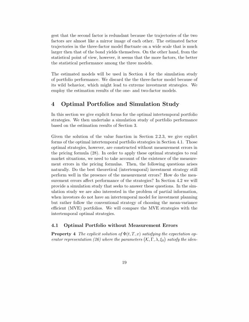
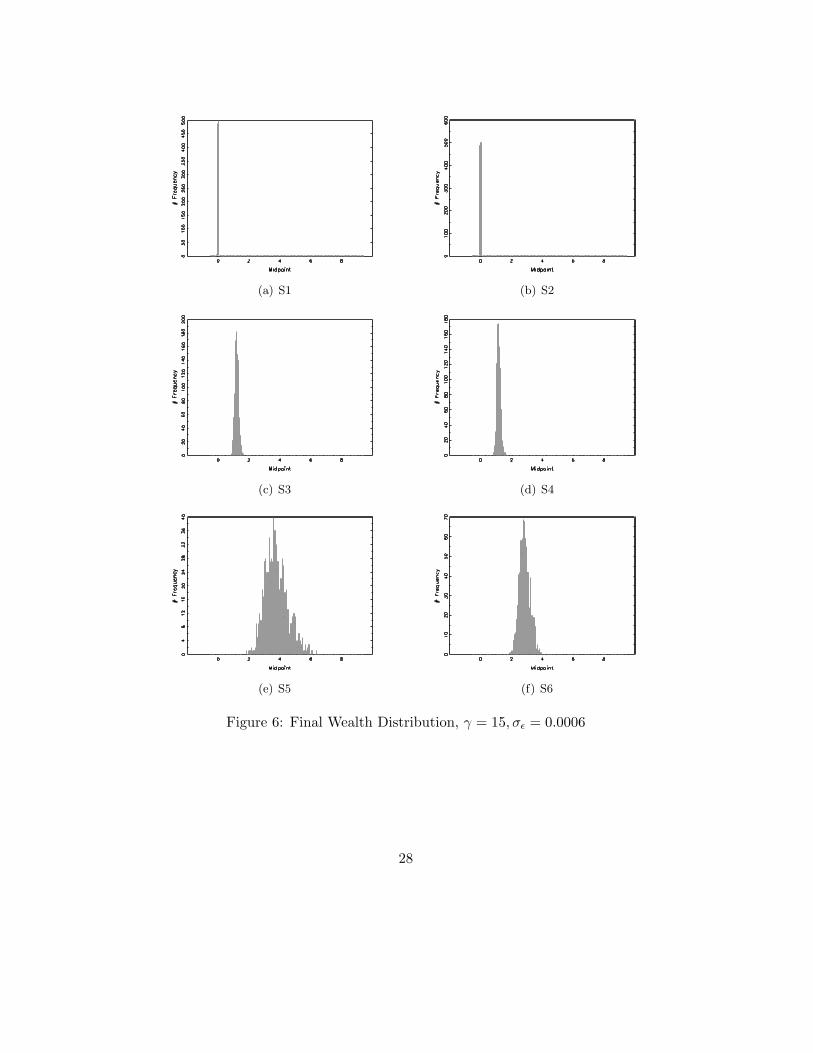
Figure 6 shows the final wealth distribution for γ = 15, where the x-axisrepresents the final wealth and the y-axis shows the frequency. Table 6 lists

25

the expected utility and the descriptive statistics of the final wealth. Recallthat the utility is always negative for the risk aversion parameter γ > 1.

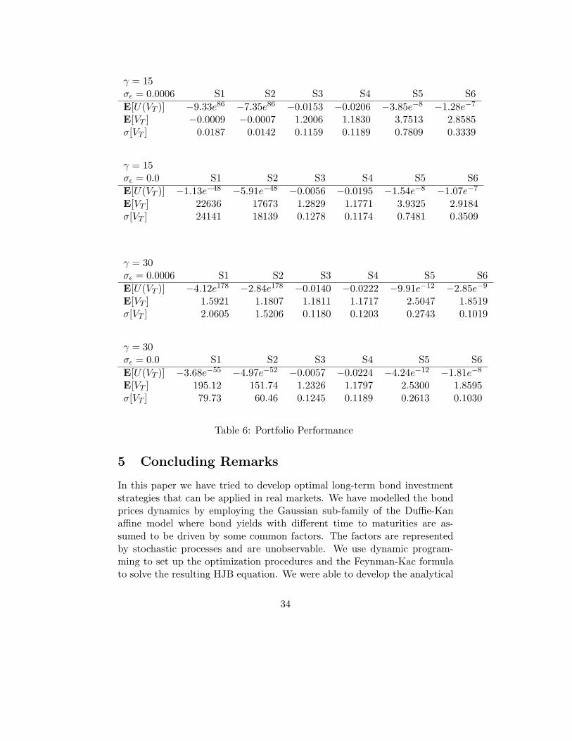
The result is quite striking because the two-factor intertemporal investmentstrategy S1, the best theoretical investment strategy, performs worst amongall strategies, in particular, much worse than the partial information strat-egy S3 and the all-money-holding strategy S4. The one-factor intertemporalinvestment strategy S5 is the winner of the this investment competition. Inthe statistical summary in Table 6 we can see that the average of the finalwealth by adopting best theoretical investment strategy S1 is even negative.This means, the agents are given one unit of wealth at the beginning ofinvestment but end up with a negative outcome of wealth in average after10 year investment following the best theoretical investment strategy!

In order to explain this outcome we trace the wealth development over thewhole investment period. Figure 7 shows one typical path of the wealth de-velopment by adopting the best theoretical investment strategy S1. We cansee in this figure that the trajectory of the wealth development undergoessteep falls at the time t = 0, 3, and 6 (year) where a new 3-year bond isintroduced. At the time t = 6 the agents’ wealth falls to a level around zeroand is not able to recover subsequently before the end of the investmenthorizon.

In Figure 8 we plot the two-factor intertemporal investment strategy S1through time. We can see that the time points of introduction of new bondsare also break points for the positions of the strategy S1. This suggeststhat the introduction of the new short-term bond causes the rapid declinein wealth.

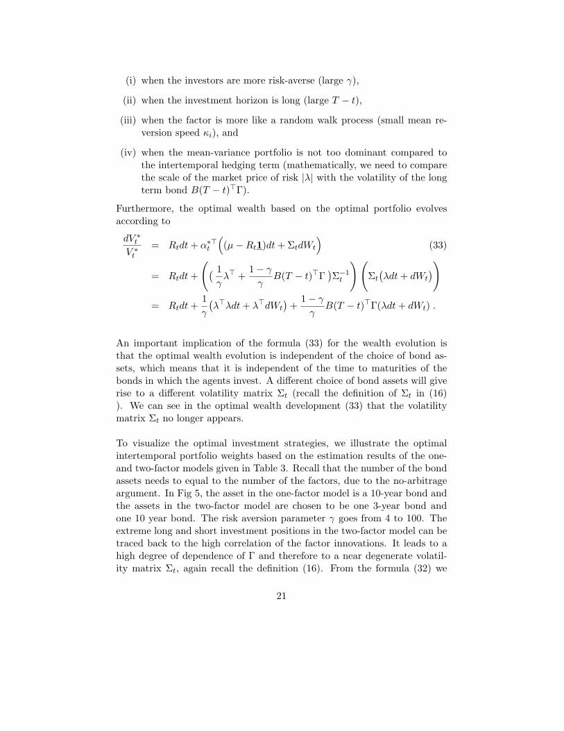
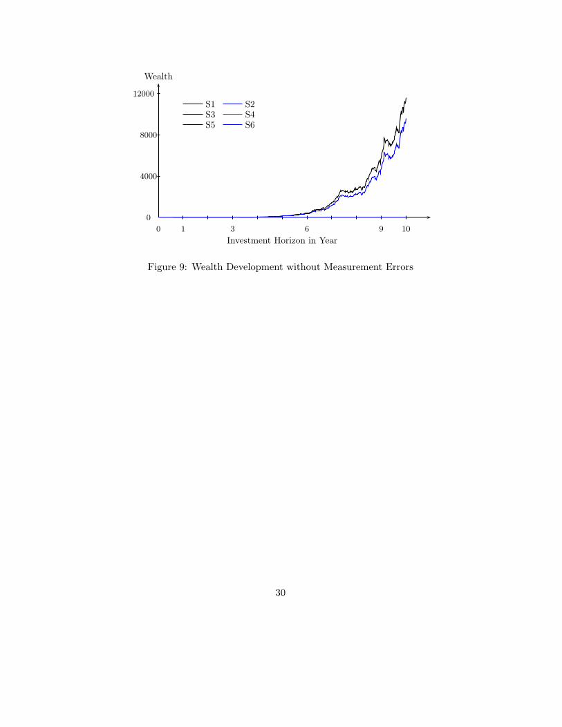
It is worth recalling here that, in the case without measurement errors, thewealth development under the optimal investment strategy is independentof the choice of bond securities, as illustrated in the optimal wealth dynam-ics (33). The impact of the introduction of the new short-term bond on thewealth development seems to be related to the existence of the measurementerrors. To highlight the impact of the measurement errors we also provideone typical path of the wealth development under the theoretical investmentstrategies in the case without the measurement errors in Figure 9. In thisfigure we see indeed that the wealth development shows no breaks at thetime of the introduction of the new bonds.

26

Figure 10 shows the final wealth distributions by adopting all six strate-gies for the case without measurement errors. From Table 6 we can see thatthe best theoretical intertemporal strategy S1 now indeed performs best interms of the expected utility E[UT ]. We also see that without measurementerrors, for all six investment strategies agents are better off. The improve-ment of the other strategies S3 – S6 is only slight.

The partial information MVE strategy S3 performs on average slightly bet-ter than the “do-nothing”, or the all-money-holding strategy S4. It has ahigher value of expected utility and a higher average return. It should benoted that the sample mean and sample standard deviation of the bond re-turns cannot appropriately approximate the drift and diffusion coefficientsin the model because the drift and diffusion vary with the time to maturity.Nevertheless, if one does not have other information, the strategy S3 whichseeks to learn the price dynamics by observing the market prices, can stillbeat the all-money-holding strategy S4.

The one-factor intertemporal investment strategy S5 performs well in bothcases with and without measurement errors. Its stable performance may betraced back to the fact that its holding position is not as extreme as thatbased on the two-factor model, as illustrated in Figure 5. On the otherhand, the agents who adopt the strategy S5 do have an intertemporal modelin mind. This is an informational advantage to the agents adopting MVEstrategies S3 and S6.

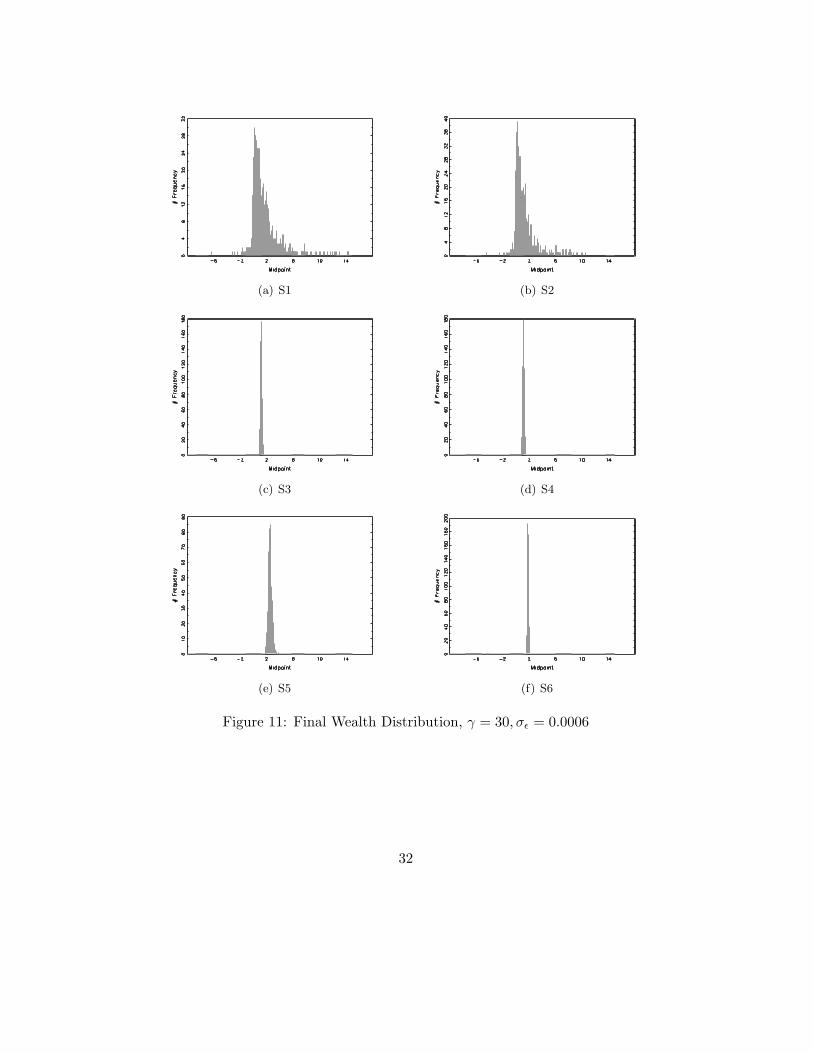
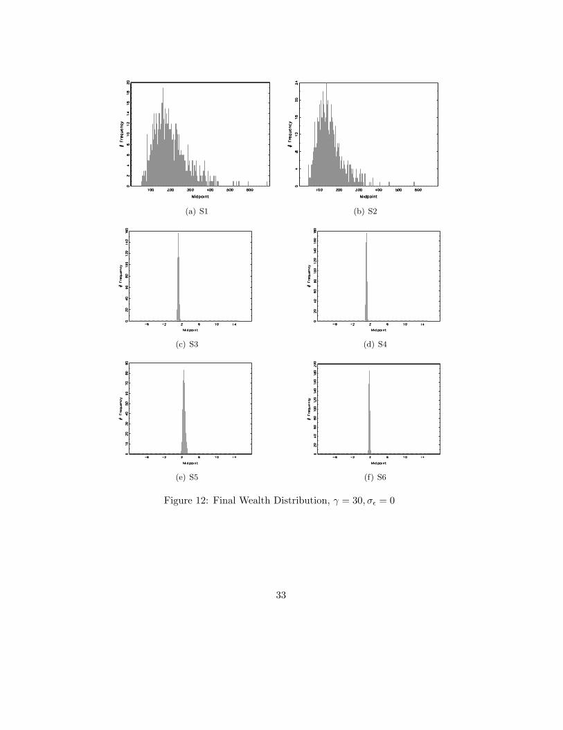
We provide also the final wealth distributions for agents with higher riskaversion γ = 30. Such agents do not take as extreme investment positionsas the agents with γ = 15, so the standard variations of the final wealth dis-tributions based on strategies S1 and S2 without measurement errors, andthose based on strategies S5 and S6 with or without measurement errors, arereduced, as shown in Table 6. This more conservative attitude also makesnegative final wealth a very low probability outcome by adopting strategiesS1 and S2 in the presence of the measurement errors, as we can observe inthe same table.

27

(a) S1 (b) S2

(c) S3 (d) S4

(e) S5 (f) S6

Figure 6: Final Wealth Distribution, γ = 15, σε = 0.0006

28

Investment Horizon in Year0 1 3 6 9 10

Wealth

0

2

4

6

S1 S2S3 S4S5 S6

Figure 7: Wealth Development with Measurement Errors

0 1 3 6 9 10

0

3000

Investment Proportionsin Short-term Bond

Investment Horizon in Year0 1 3 6 9 10

in Long-term Bond

-300

0

300

Figure 8: Theoretical Intertemporal Portfolio Proportions

29

Investment Horizon in Year0 1 3 6 9 10

Wealth

0

4000

8000

12000

S1 S2S3 S4S5 S6

Figure 9: Wealth Development without Measurement Errors

30

(a) S1 (b) S2

(c) S3 (d) S4

(e) S5 (f) S6

Figure 10: Final Wealth Distribution, γ = 15, σε = 0

31

(a) S1 (b) S2

(c) S3 (d) S4

(e) S5 (f) S6

Figure 11: Final Wealth Distribution, γ = 30, σε = 0.0006

32

(a) S1 (b) S2

(c) S3 (d) S4

(e) S5 (f) S6

Figure 12: Final Wealth Distribution, γ = 30, σε = 0

33

γ = 15σε = 0.0006 S1 S2 S3 S4 S5 S6E[U(VT )] −9.33e86 −7.35e86 −0.0153 −0.0206 −3.85e−8 −1.28e−7

E[VT ] −0.0009 −0.0007 1.2006 1.1830 3.7513 2.8585σ[VT ] 0.0187 0.0142 0.1159 0.1189 0.7809 0.3339

γ = 15σε = 0.0 S1 S2 S3 S4 S5 S6E[U(VT )] −1.13e−48 −5.91e−48 −0.0056 −0.0195 −1.54e−8 −1.07e−7

E[VT ] 22636 17673 1.2829 1.1771 3.9325 2.9184σ[VT ] 24141 18139 0.1278 0.1174 0.7481 0.3509

γ = 30σε = 0.0006 S1 S2 S3 S4 S5 S6E[U(VT )] −4.12e178 −2.84e178 −0.0140 −0.0222 −9.91e−12 −2.85e−9

E[VT ] 1.5921 1.1807 1.1811 1.1717 2.5047 1.8519σ[VT ] 2.0605 1.5206 0.1180 0.1203 0.2743 0.1019

γ = 30σε = 0.0 S1 S2 S3 S4 S5 S6E[U(VT )] −3.68e−55 −4.97e−52 −0.0057 −0.0224 −4.24e−12 −1.81e−8

E[VT ] 195.12 151.74 1.2326 1.1797 2.5300 1.8595σ[VT ] 79.73 60.46 0.1245 0.1189 0.2613 0.1030

Table 6: Portfolio Performance

5 Concluding Remarks

In this paper we have tried to develop optimal long-term bond investmentstrategies that can be applied in real markets. We have modelled the bondprices dynamics by employing the Gaussian sub-family of the Duffie-Kanaffine model where bond yields with different time to maturities are as-sumed to be driven by some common factors. The factors are representedby stochastic processes and are unobservable. We use dynamic program-ming to set up the optimization procedures and the Feynman-Kac formulato solve the resulting HJB equation. We were able to develop the analytical

34

solution for the intertemporal optimal strategies for the bond investments.

The model was estimated based on the data from German securities marketsusing the Kalman filter. Although the three-factor term structure model hasthe largest fitting errors and the smallest information criteria, we did notemploy it because of the widely fluctuating trajectories of the filtered fac-tors. Thus, we employed the one- and the two-factor term structure modelsto develop bond investment strategies.

Using the analytical solution obtained for the intertemporal optimal port-folios, we showed that the two models give very different recommendationsfor bond investment strategies. The best theoretical investment strategy,which is based on the estimation results of the two-factor model, tends togive a strategy with extremely large investment positions because of the highcorrelation of the factor innovations. With regard to this point, the resultsof the simulation study have revealed the fact that an investment strategywith such large positions is very vulnerable to measurement errors.

In the simulation study we simulated the bond prices based on the esti-mateion results of the two-factor term structure model and investigated theperformance of six different investment strategies: the two-factor intertem-poral strategy S1, the two-factor MVE strategy S2, the partial informationMVE strategy S3, the all-money-holding strategy S4, the one-factor intert-meporal strategy S5, and the one-factor MVE strategy S6, in the scenar-ios with and without measurement errors. The best theoretical investmentstrategy S1 performs the worst among all the strategies in the presence ofthe measurement errors because of their large long/short positions. Thepartial information MVE strategy S3 performed only slightly better thanthe all-money-holding strategy S2 because the sample mean and varianceare not a good proxy for the time-varying drift and diffusion of the bondreturns.

The one-factor intertemporal strategy S5 stood out in our simulation studybecause of its stable and relatively good performance for both cases withand without the measurement errors. The success might be explained bytwo features of this strategy that come together: on the one hand, it in-corporate the information of the time-changing investment environment; onthe other hand, the investment positions are of a reasonable scale.

The approach of this paper can be extended in several ways in future re-

35

search. For example, we could include stocks in order to study the interac-tion between stocks and bonds in the intertemporal asset allocation problem.Intermediate consumption has not yet been considered in this study and willbe the object of future research.

6 Appendix

6.1 Proof

The characterization of the invariant transformation of the parameters hasalready been stated in Dai and Singleton (2000) . Here we provide a moredetailed proof.

Lemma 4.1 (Dai and Singleton (2000)) The invariant transformation ofthe parameters

(K, θ, Γ, ξ0, ξ1

)of equations (2), (5), (9) and (10) with respect

to the factor transformation

XLt := LXt + Θ (40)

is given by (LKL−1, Lθ + Θ, LΓ, ξ0 − ξ�1 L−1Θ, (L�)−1ξ1

). (41)

ProofThe first three invariant parameter transformation can be determined easily.We denote KL, θL, ΓL as the new parameters for the new factor dynamics

dXLt = KL(θL − XL

t )dt + ΓLdWt . (42)

Under the factor transformation (40), the new factor dynamics can be trans-formed into

dXLt = LdXt = LK(θ − Xt)dt + LΓdWt

= LK(θ − L−1(LXt + Θ) + L−1Θ)dt + LΓdWt

= (LKL−1)(Lθ + Θ − XL

t

)dt + LΓdWt . (43)

Identifying the two dynamical systems (42) and (43), we obtain

KL = LKL−1 , (44)θL = Lθ + Θ ,

ΓL = LΓ .

36

Let BL(τ), AL(τ) be the new coefficients in the yield formula (2) based onthe transformed factor XL

t . The invariant transformation must satisfy tworequirements. First, the bond formulas must remain invariant under thetransformation, so that

y(t, t + τ, Xt) =A(τ)

τ+

B(τ)�

τXt ≡ AL(τ)

τ+

BL(τ)�

τXL

t . (45)

Replacing the new factor XLt in equation (45) with its definition given in

(40), we obtain for the new coefficients BL(τ) and AL(τ) the equalities

BL(τ)� = B(τ)�L−1 , (46)A(τ) = AL(τ) + B(τ)�L−1Θ . (47)

The second requirement for the invariant transformation is that the newcoefficient BL(τ) and AL(τ) must still satisfy the no-arbitrage equations (9)and (10) with the new parameters given in (44). That is, the coefficientBL(τ) must satsify

d

dτBL(τ) = −(KL)�BL(τ) + ξL1 = −(L−1)�K�L�BL(τ) + ξL1 .

Multifying L� on both sides, we obtain

d

dτ

(L�BL(τ)

)= −K�L�BL(τ) + L�ξL1 .

This equation can be simplified further to

d

dτB(τ) = −K�B(τ) + ξL1 , (48)

due to the fact L�BL(τ) ≡ B(τ) from the equality (46).

Identifying the new differential equation (48) for BL(τ) with the original one(9), it turns out that the new parameter ξL1 must satisfy

L�ξL1 = ξ1 . (49)

Applying the second requirement also to the coefficient AL(τ), it has tosatisfy the no-arbitrage condition (10) with the new parameters (44) andthe new coefficient BL(τ), thus

d

dτAL(τ) =

(KLθL − ΓLλ)�

BL(τ) − 12

n∑i,j=1

BLi (τ)BL

j (τ)ΓLi ΓL

j + ξL0 . (50)

37

We can observe thatn∑

i,j=1

BLi (τ)BL

j (τ)ΓLi ΓL

j =(BL(τ)�ΓL)(BL(τ)�ΓL)� =

(B(τ)�Γ

)(B(τ)�Γ

)�.

Applying this equalty and the definitions of new parameters given in (44)to the differential equation (50), then it can be rewritten further to

d

dτAL(τ) = (Kθ + KL−1Θ − Γλ)�B(τ) − 1

2

n∑i,j=1

Bi(τ)Bj(τ)ΓiΓj + ξL0

=d

dτA(τ) + (KL−1Θ)�B(τ) + ξL0 − ξ0 . (51)

The second equality above is obtained by using the original no-arbitragecondition (10).

Now, we differentiate both sides of (47) and then replace ddτ B(τ) by the

original no-arbitrage condition (9), then we obtain

d

dτA(τ) =

d

dτAL(τ) +

d

dτB(τ)�L−1Θ

=d

dτAL(τ) + (−B(τ)�K + ξ�1 )L−1Θ . (52)

Identifying the two equations (51) and(52), it follows that the new parameterξL0 has to satisfy

ξL0 = ξ0 − ξ�1 LΘ . (53)

We note that the price of risk λ remains unchanged under the factor trans-formation because we keep the original factor uncertainty Wt. We recallthat the price of risk is the compensation for bearing the uncertainty Wt.�

Proof of Property 2Because K is diagonal, we can solve every component of the coefficient B(τ)separately. Together with Condition (iii) in Property 1, the i-th componentof B(τ) has to satisfy

d

dτBi(τ) = −κiBi(τ) + 1 , (54)

from which the solution (11) follows readily by applying the integration fac-tor eκiτ and the initial condition Bi(0) = 012.

12Equation (54) is sloved by applying the intergrating factor eκiτ and rewritting it as

eκiτ ` d

dτBi(τ) + κiBi(τ)

´=

d

dτ

`eκiτBi(τ)

´= eκiτ ,

38

The solution given in (12) is simpliply obtained by subsituting the expres-sion (11) into the terms in (10) and then integrating.�

Proof of Property 3

The proof proceeds in two steps.

1: Change of probability measure

Let P denote the original, so called physical or historical, probability mea-sure for the underlying process (5). Now, a new equivalent measure is definedby the Radon-Nikodym derivative

dPs

dPs= exp

(1 − γ

γλ�(Ws − Wt) − (1 − γ)2

2γ2λ�λ(s − t)

).

Using Girsanov’s theorem, the shifted Brownian motion

dWt = dWt − 1 − γ

γλdt

is a Brownian motion under the new measure P.Inserting the shifted Brownian motion into the original underlying process(5), we obtain the stochastic differential equation

dXt = K(θ − Xt)dt + ΓdWt

=(K(θ − Xt) + Γ

1 − γ

γλ)dt + ΓdWt . (55)

2: Application of the Feynman-Kac formula

By applying the Feynman-Kac formula, see the Theorem 1 in the Appendix6.2, we obatin the result (26).�

Proof of Property 4

Inserting the expressions for ht into (24) and the Radon-Nikodym derivative

which is readily integrated.

39

in (27) into the expectation operator representation (26), we obtain

Φ(t, T, x) = Et,x[eΨ(t,T )] , (56)

where we use Ψ(t, T ) to denote

Ψ(t, T ) := − δ

γ(T − t) +

1 − γ

2γ2λ�λ(T − t) +

1 − γ

γ

∫ T

tRsds

+1 − γ

γλ�(WT − Wt) − (1 − γ)2

2γ2λ�λ(T − t)

= − δ

γ(T − t) +

1 − γ

2γλ�λ(T − t) +

1 − γ

γλ�(WT − Wt)

+1 − γ

γξ0(T − t) +

n∑i=1

1 − γ

γ

∫ T

tXisds . (57)

The second equality in equation (57) is due to the fact that

Rs = ξ0 +n∑

i=1

Xis,

which is based on the result (3) and the identification restriction (iii) inProperty 1. Note that the process Xis is the i-th component of the factorXs.

Since the matrix K is diagonal due to the identification restriction (i) inProperty 1, the underlying process (5) can be expressed componentwise as

dXis = κi(θi − Xis)ds + ΓidWs .

The solution of the stochastic differential equation above is given by13

Xis = e−κi(s−t)Xit +∫ s

te−κi(s−u)ΓidWu .

So, the last term of the equation (57) becomes∫ T

tXisds =

∫ T

te−κi(s−t)Xitds +

∫ T

t

∫ s

te−κi(s−u)ΣidWuds

=1κi

(1 − e−κi(T−t))Xit +∫ T

t

∫ T

ue−κi(s−u)dsΣidWu

= Bi(T − t)Xit +∫ T

tBi(T − u)ΣidWu .

13See Kloeden and Platen (1992) .

40

Using this result to rewrite equation (57), we obtain

Ψ(t, T ) = − δ

γ(T − t) +

1 − γ

2γλ�λ(T − t) +

1 − γ

γξ0(T − t)

+B(T − t)Xt +∫ T

t

(B(T − u)�Σ + λ�)dWu .

It is easy to see that Ψ(t, T ) is normally distributed with the expectation

EΨ(t, T ) = − δ

γ(T − t) +

1 − γ

2γλ�λ(T − t) +

1 − γ

γξ0(T − t) + B(T − t)Xt

and the variance

VarΨ(t, T ) =∫ T

t

(B(T − u)�Σ + λ�)(B(T − u)�Σ + λ�)�ds .

Using the well-known result concerning the expected value of the exponentialof a normally distributed random variable, we obtain from (56) that

Φ(t, T, x) = Et,x[eΨ(t,T )] = eEΨ(t,T )+ 12VarΨ(t,T ) ,

which is equivalent to the expression (30) in Property 4.�

6.2 Some Basic Results

Theorem 1 (Feynman-Kac Formula) Let Xt be the solution of the stochas-tic differential equation (SDE)

dXt = Ftdt + GtdWt (58)

the infinitesimal generator of which is given by

Dt = F�t

∂

∂x+

12

n∑i,j=1

GitG�jt

∂

∂xi

∂

∂xj.

Let h, g, and Ψ are functions with dimentionality h : Rd × R+ → R, g :

Rd × R+ → R, and Ψ : R

d × R+ → R. If Ψ(x, t) satisfies the PDE

∂

∂tΨ(x, t) + DtΨ(x, t) + h(x, t)Ψ(x, t) + l(x, t) = 0 , (59)

41

subject to the boundary condition

Ψ(x, T ) = ω(x) , (60)

then

Ψ(x, t) = Et,x

[ω(XT )e

R Tt h(Xs,s)ds +

∫ T

tl(Xs, s)e

R st h(Xu,u)duds

], (61)

where Et,x is the expectation operator with respect to the stochastic processXs, s ≥ t satisfying the SDE (58) with initial position Xt = x.

For the proof of the Feymann-Kac formula, see, for example, Øksendal(2003) or Korn (1997).�

Kalman Filter

The Kalman filter is employed to estimate the model consisting of one ob-servation equation

yt = ZtXt + dt + εt , (62)

and one state equation

Xt = TtXt−1 + ct + Rtηt . (63)

The notation is adopted from Harvey(1990). For each t, the N ×1-vector yt

is directly observable. On the right hand side of (62) the observations areexplained by an observable component dt and the unobservable state variableXt. The state variable follows the dynamics (63). The Kalman filter canestimate the unobservable Xt based on the information/observations untilt. Further details of the Kalman filter may obtained in Harvey(1990).

42

References

[1] Brennan, M.J., E.S. Schwartz, and R. Lagnado. Strategic asset alloca-tion. Journal of Economic Dynamics and Control, 21:1377–1403, 1997.

[2] Brennan, M.J., A.W. Wang, and Y. Xia. Estimation and test of asimple model of intertemporal capital asset pricing. The Journal ofFinance, 59(4):1743–75, August 2004.

[3] Brennan, M.J. and Y. Xia. Dynamic asset allocation under inflation.The Journal of Finance, 57(3):1201–1238, 2002.

[4] Burnham, K.P. and D.R. Anderson. Multimodel Inference: understand-ing AIC and BIC in Model Selection. Amsterdam Workshop on ModelSelection, Internet Source, 2004.

[5] Campbell, J.Y. and L.M. Viceira. Strategic Asset Allocation. OxfordUnivery Press, 2002.

[6] Chiarella, C. An Introduction to Derivative Security Pricing, Lecturenotes UTS, 2004.

[7] Cox, J.C. and C-F. Huang. Optimal consumption and portfolio poli-cies when asset prices follow a diffusion process. Journal of EconomicTheory, 49:33–83, 1989.

[8] Cox, J.C., J.E. Ingersoll, and S.A. Ross. An intertemporal generalequilibrium model of asset prices. Econometrica, 53(2):363–384, March1985.

[9] Cox, J.C., J.E. Ingersoll, and S.A. Ross. A theory of the term structureof interest rates. Econometrica, 53(2):385–407, March 1985.

[10] Dai, Q. and K. Singleton. Specification analysis of affine term structuremodels. Journal of Finance, 55:1943–78, 2000.

[11] Duffie, D. and R. Kan. A yield-factor model of interest rates. Mathe-matical Finance, 6(4):397–406, 1996.

[12] Harvey, A.C. Forecasting, Structural Time Series Models and theKalman Filter. Cambridge, 1990.

[13] Hsiao C.Y. Intertemporal Asset Allocation under Inflation Risk. PhDThesis, Bielefeld University, Germany, forthcoming 2006.

43

[14] Kamien, M.I. and N.L. Schwartz. Dynamic Optimization. North-Holland, 1991.

[15] Kim, T.S. and E. Omberg. Dynamic nonmyopic portfolio behavior. TheReview of Financial Studies, 9(1):141–161, 1996.

[16] Kloeden, P.E. and E. Platen. Numerical Solution of Stochastic Differ-ential Equations. Springer, 1992.

[17] Korn, R. Optimal Portfolios. World Scientific, 1997.

[18] Lintner, J. The valuation of risk assets and the selection of risky invest-ments in stock portfolios and capital budegts. The Review of Economicsand Statistics, 47:13–37, 1965.

[19] Liu, J. Portfolio selection in stochastic environments. Standford GSBWorking Papers; forthcoming, Review of Financial Studies, 2005.

[20] Liu, J. and J. Pan. Dynamic derivative strategies. Journal of FinancialEconomics, 69:401–430, 2003.

[21] Markowitz, H.M. Portfolio Selection. Yale University Press, 1959.

[22] Merton, R.C. Optimum consumption and portfoliio rules in acontinuous-time model. Journal of Economic Theory, 3:373–413, 1971.

[23] Merton, R.C. An intertemporal capital asset pricing model. Economet-rica, 41(5):867–887, 1973.

[24] Merton, R.C. Continuous Time Finance. Blackwell, 1990.

[25] Munk, C., C. Sørensen, and T.N. Vinther. Dynamic asset allocationunder mean-reverting returns, stochastic interest rates and inflationuncertainty: Are popular recommdendations consistent with rationalbehavior? International Review of Economics and Finance, 13(141-166), 2004.

[26] Øksendal, B. Stochastic Differential Equations. Springer, 6 edition,2003.

[27] Sharpe, W.F. Capital asset prices: A theory of market equilibriumunder conditions of risk. The Journal of Finance, 19(3):425–442, 1964.

44