intertemporal cost allocation and investment...

Intertemporal Cost Allocation and Investment DecisionsAuthor(s): William P. RogersonReviewed work(s):Source: Journal of Political Economy, Vol. 116, No. 5 (October 2008), pp. 931-950Published by: The University of Chicago PressStable URL: http://www.jstor.org/stable/10.1086/591909 .

Accessed: 08/01/2013 10:41

Your use of the JSTOR archive indicates your acceptance of the Terms & Conditions of Use, available at .http://www.jstor.org/page/info/about/policies/terms.jsp

.JSTOR is a not-for-profit service that helps scholars, researchers, and students discover, use, and build upon a wide range ofcontent in a trusted digital archive. We use information technology and tools to increase productivity and facilitate new formsof scholarship. For more information about JSTOR, please contact [email protected].

.

The University of Chicago Press is collaborating with JSTOR to digitize, preserve and extend access to Journalof Political Economy.

http://www.jstor.org

This content downloaded on Tue, 8 Jan 2013 10:41:15 AMAll use subject to JSTOR Terms and Conditions

http://www.jstor.org/action/showPublisher?publisherCode=ucpress

http://www.jstor.org/stable/10.1086/591909?origin=JSTOR-pdf

http://www.jstor.org/page/info/about/policies/terms.jsp


931

[ Journal of Political Economy, 2008, vol. 116, no. 5]� 2008 by The University of Chicago. All rights reserved. 0022-3808/2008/11605-0002$10.00

Intertemporal Cost Allocation and InvestmentDecisions

William P. RogersonNorthwestern University

This paper considers the profit-maximization problem of a firm thatmust make sunk investments in long-lived assets to produce output.It is shown that if per-period accounting income is calculated usinga simple and natural allocation rule for investment, called the relativereplacement cost (RRC) rule, under a broad range of plausible cir-cumstances, the firm can choose the fully optimal sequence of in-vestments over time simply by choosing a level of investment eachperiod in order to maximize the next period’s accounting income.Furthermore, in a model in which shareholders delegate the invest-ment decision to a better-informed manager, it is shown that if ac-counting income based on the RRC allocation rule is used as a per-formance measure for the manager, robust incentives are created forthe manager to choose the profit-maximizing sequence of investments,regardless of the manager’s own personal discount rate or other as-pects of the manager’s personal preferences.

I. Introduction

In a variety of industries, firms must make sunk investments in long-lived assets to produce output. Calculation of profit-maximizing invest-ment levels and evaluation of the firm’s performance in such a situationare inherently complicated because of the need to consider implicationsfor cash flows over multiple future periods. One technique that firmsroutinely use to create simplified single-period “snapshots” of their per-formance is to calculate per-period accounting income using accounting

I would like to thank Debra Aron, Kathleen Hagerty, Stefan Reichelstein, Korok Ray,David Sappington, William Sharkey, Nancy Stokey, T. N. Srinivasan, Jean Tirole, and threeanonymous referees for helpful discussions and comments.



932 journal of political economy

measures of cost that allocate the costs of purchasing long-lived assetsover the periods that the assets will be used. Firms use these single-period snapshots of performance both to directly guide their investmentdecisions and to evaluate the performance of managers who make in-vestment decisions. Given their widespread use to both directly andindirectly guide investment decisions, it is perhaps surprising that therehas been almost no formal analysis in the economics, finance, or ac-counting literature that attempts to investigate whether there is any basisfor these accounting practices and, if so, how the choice of an allocationrule ought to be affected by factors such as the pattern of depreciationof the underlying asset, the firm’s discount rate, the rate at which assetprices are changing over time, and the manager’s own rate of timepreference. This paper provides a theory that addresses these questions.It shows that, under a broad range of plausible circumstances, a naturaland simple allocation rule, which will be called the relative replacementcost (RRC) rule, can be used both to simplify calculation of the optimallevel of investment and to create robust incentives for managers tochoose this level of investment when the decision is delegated to them.

In particular, two major results are proven. First, it is shown that,when accounting income is calculated using the RRC allocation rule,the firm can choose the fully optimal sequence of investments simplyby choosing a level of investment each period in order to maximize thenext period’s accounting income. Second, in a model in which share-holders delegate the investment decision to a better-informed manager,it is shown that if shareholders base the manager’s wage each periodon current and past periods’ accounting income calculated using theRRC rule, the manager will have the incentive to choose the fully optimalsequence of investments as long as each period’s wage is weakly in-creasing in current and past periods’ accounting income. Furthermore,this result holds regardless of the manager’s own personal discount rateor other aspects of the manager’s personal preferences. Therefore, theinvestment incentive problem is solved in a robust way, and the firm isleft with considerable degrees of freedom to address any other incentiveproblems that may exist, such as providing incentives for the managerto exert effort each period, by choosing the precise functional form ofthe wage function each period.

In the formal model of this paper, it is assumed that assets have aknown but arbitrary depreciation pattern and that the purchase priceof new assets changes at a known constant rate over time. The RRCallocation rule is defined to be the unique allocation rule that satisfiesthe following two properties: (i) the cost of purchasing an asset is al-located across periods of its lifetime in proportion to the relative costof replacing the surviving amount of the asset with new assets, and (ii)



intertemporal cost allocation and investment 933

the present discounted value of the cost allocations using the firm’sdiscount rate is equal to the initial purchase price of the asset.

Property i can be interpreted as a version of the “matching principle”from accrual accounting that states that investment costs should beallocated across periods so as to match costs with benefits, where the“benefit” that an asset contributes to any period is interpreted to be theavoided cost of purchasing new capacity in that period. Property ii canbe viewed as stating that the investment should be fully allocated, takingthe time value of money into account. Most traditional accounting sys-tems ignore the time value of money when allocating investment costsover time. The term “residual income” is generally used in the account-ing literature to describe income measures that are calculated using anallocation rule for investment that takes the time value of money intoaccount (Horngren and Foster 1987, 873–74). Recently there has beenan explosion of applied interest in using residual income both to directlyguide capital budgeting decisions and as a performance measure formanagers who make capital budgeting decisions. Management con-sulting companies have renamed this income measure “economic valueadded” (EVA) and very successfully marketed it as an important newtechnique for maximizing firm value. Fortune, for example, has run acover story on EVA, extolling its virtues and listing a long string of majorcompanies that have adopted it (Tully 1993).1 This paper provides anexplicit formal model that justifies the use of residual income in thecapital budgeting process and also specifically identifies the particularallocation rule that should be used to calculate residual income andhow it depends on the depreciation pattern of the underlying assets.

Most of the literature on the optimal investment problem under cer-tainty restricts itself to considering the case of exponential depreciation,in which a constant share of the capital stock is assumed to depreciateeach year regardless of the age profile of the capital stock.2 The as-sumption of exponential depreciation dramatically simplifies the anal-ysis because the age profile of the existing capital stock can be ignored.However, for the purposes of this paper’s study of cost allocation rules,it is important to allow for general patterns of depreciation because oneof the most interesting questions to investigate regarding cost allocationrules is how the nature of the appropriate cost allocation rule shouldchange as the depreciation pattern of the underlying assets changes.Obviously the pattern of depreciation must be a factor that can beexogenously varied in order to investigate this question. Furthermore,the case of exponential depreciation is not a particularly natural case

1 See the roundtable discussion in the Continental Journal of Applied Corporate Finance(Stern and Stewart 1994) and the associated articles (Sheehan 1994; Stewart 1994).

2 See Jorgensen (1963) for an early analysis, and see Abel (1990) for a more extensivediscussion of the optimal investment literature and further references.




to consider for most real applications. In most real applications, a muchmore natural case to consider is the so-called case of “one-hoss shay”depreciation, in which assets are assumed to have finite lifetimes andto remain equally productive over their lifetimes. This paper’s analysisof the general case will, in particular, apply to the case of one-hoss shaydepreciation.

This paper’s results are based on Arrow’s (1964) analysis of the op-timal investment problem under certainty for general patterns of de-preciation. Arrow shows that for any given depreciation pattern of assets,a vector of “user costs” can be calculated with the property that, undera broad range of plausible circumstances, the seemingly complex op-timal investment problem collapses into a series of additively separablesingle-period problems by which the firm can be viewed as choosingthe amount of capital to “rent” each period with rental rates given bythe vector of user costs. This paper’s basic insight is that a simple costallocation rule (namely, the RRC rule) can be defined with the propertythat the cost it allocates to any period of an asset’s lifetime is equal tothe surviving amount of the asset multiplied by that period’s user cost.The desirable properties of the RRC rule then follow from this. As partof the proof that the RRC allocation rule has this relationship to usercost, this paper derives a different and much simpler formula for cal-culating user cost than the formula derived by Arrow. In particular,Arrow’s formula for calculating user cost depends on the vector of mar-ginal investment rates, which describe the series of changes in invest-ments sufficient to increase the stock of capital by one unit in a givenperiod while holding the stock of capital constant in all other periods.For the case of general depreciation patterns, the formula for the vectorof marginal investment rates is complicated and difficult to calculateand is defined by an infinite series of recursively defined functions. Thispaper shows that it is possible to derive an alternate and much simplerformula for user cost that does not depend on marginal investmentrates.3 In particular, it shows that a very simple formula exists to calculatehypothetical, perfectly competitive rental prices for assets and thenproves that these hypothetical, perfectly competitive rental prices mustbe equal to user costs. The fact that user cost can be calculated by avery simple formula that does not depend on marginal investment ratesis an interesting result independent of its application to cost allocationrules. Furthermore, the fact that user costs can be interpreted as hypo-

3 For the special case of exponential depreciation, the formula that determines marginalinvestment rates is very simple, and Arrow observes that his formula for user cost collapsesinto the simple formula directly derived by Jorgensen (1963) for this case. The incrementalcontribution of this paper is to show that a similarly simple formula to calculate user costsexists for general depreciation patterns even when there is no simple formula to calculatethe vector of marginal investment rates.




thetical, perfectly competitive rental prices provides some extra eco-nomic intuition to explain the user cost result.

Two recent groups of papers have considered the role of accountingmeasures of income in the capital budgeting process. Anctil (1996) andAnctil, Jordan, and Mukherji (1998) consider a model in which depre-ciation is exponential, there are adjustment costs to changing the sizeof the capital stock, and the environment is stationary. They show thatthe time path of capital stock when the firm chooses each period’scapital stock to maximize that period’s residual income converges tothe fully optimal time path. Rogerson (1997) considers a model in whichthe firm only invests once at the beginning of the first period.4 Anallocation rule called the relative benefits rule is shown to have the samesorts of desirable properties that the RRC allocation rule is shown tohave in the model of this paper. While the allocation rules identifiedby both papers can be interpreted as allocating investment costs acrossperiods in proportion to the relative benefit that the investment createsacross periods, the relevant notion of “benefit” turns out to be verydifferent in each case. In particular, in the one-time investment modelof Rogerson (1997), the optimal allocation rule is determined solely bythe demand-side factor of how the level of demand varies across periods.In contrast, the optimal allocation rule in the model of this paper isdetermined solely by the supply-side factor of how investments made indifferent periods can substitute for one another in creating capital stockto be used in a given period. In particular, the optimal allocation ruledoes not depend on how demand varies over time. Therefore the eco-nomic factors that determine the optimal allocation rule are quite dif-ferent depending on whether or not investments in different periodssubstitute for one another.

In a companion paper to this one (Rogerson 2008), it is shown thatthe approach of this paper can also be applied to the issue of calculatingwelfare-maximizing prices for a regulated firm. In particular, it is shownthat when there are constant returns to scale within each period (i.e.,when output in each period is proportional to the capital stock in eachperiod), the accounting cost of output calculated using the RRC allo-cation rule is equal to long-run marginal cost. Therefore, prices set equalto accounting cost calculated using the RRC rule are first-best in thesense that they both induce efficient consumption decisions and allowthe firm to break even.

The paper is organized as follows. Section II presents the model andArrow’s user cost result. Section III proves that the vector of user costs

4 See Rogerson (1992) for an earlier, related result. Papers that have generalized Rog-erson’s (1997) result and applied it in a number of different settings include Reichelstein(1997, 2000), Dutta and Reichelstein (1999, 2002), Baldenius and Ziv (2003), and Bal-denius and Reichelstein (2005).




can be interpreted as a vector of hypothetical, perfectly competitiverental prices and uses this to construct a simple formula for user cost.Section IV defines cost allocation rules and shows that the RRC allo-cation rule has the property that it sets the accounting cost of using aunit of capital in any period of its lifetime equal to user cost. SectionsV and VI describe the properties of the RRC allocation rule that followfrom this. Section VII briefly explains how the results generalize to thecase where future asset prices do not change at a constant rate. Moretechnical proofs are contained in the appendix.

II. The Model and Arrow’s User Cost Result

Let denote the number of assets that the firm purchases inI � [0, �)t

period . Let denote the entire vector of in-t � {0, 1, …} I p (I , I , …)0 1

vestments. Assume that assets become available for use one period afterthey are purchased and then gradually wear out or depreciate over time.It will be convenient to use notation that directly defines the share ofthe asset that survives and is thus available for use in each period, ratherthan the share that depreciates. Let denote the share of an asset thatst

survives until at least the tth period of the asset’s lifetime and let s pdenote the entire vector of survival shares. Assume that(s , s , …) s �1 2 t

for every t, , and that st is weakly decreasing in t. Two natural[0, 1] s p 11

and simple examples of depreciation patterns are the cases of expo-nential depreciation given by

t�1s p b (1)t

for some and one-hoss shay depreciation given byb � (0, 1)

1, t � {1, 2, … ,T }s p (2)t {0, otherwise,

where T is a positive integer.For simplicity, assume that the firm begins period 0 with no existing

capital.5 Let Kt denote the number of assets the firm has available foruse in period and let denote the entiret � {1, 2, …} K p (K , K , …)1 2

5 All of the analysis in this paper actually applies to the general case where the firmenters period 0 with existing assets if Kt is interpreted as the firm’s incremental capitalstock, that is, its capital stock created by assets purchased in period 0 or later.




vector of capital stocks. The vector of capital stocks generated by anyvector of investments is then determined by the linear mapping6

K p [S]I, (3)

where [S] is the lower triangular matrix

s 0 0 …1

s s 0 …2 1[S] p . (4)s s s …3 2 1

_ _ _

It is evident by inspection that [S] is invertible and that its inverse isthe matrix [M] defined by

m 0 0 …0

m m 0 …�1 1 0[S] p [M] p , (5)m m m …2 1 0

_ _ _

where the values of mi are determined sequentially by

m p 1, (6)0

i

m s p 0 for i � {1, 2, …}. (7)� j i�1�jjp0

Therefore, the unique vector of investments that generates any givenvector of capital stocks is determined by the linear mapping

I p [M]K. (8)

The mi parameters have a very natural interpretation. Suppose that thefirm wishes to increase its stock of capital in period t by one unit whileleaving the capital stock in all other periods fixed. Then mi is the mar-ginal adjustment to investment that the firm must make in period t �

. The vector will be called the vector of marginal1 � i m p (m , m , …)0 1

investment rates.Let denote the firm’s discount rate. Let denoted � (0, 1) p � [0, �)t

the price of purchasing a new unit of the asset in period t, and letdenote the vector of all asset prices. It will always bep p (p , p , …)0 1

assumed that ptdt is decreasing in t, so that it is not profitable to stockpile

assets ahead of time. Many of the results in this paper will require the

6 I would like to thank Nancy Stokey for suggesting that I present the main argumentsusing matrix notation, which dramatically simplifies and clarifies the analysis. When matrixnotation is used, vectors will be interpreted to be column vectors, and row vectors will bedenoted by the superscript T.




additional assumption that asset prices change at a constant rate overtime, that is, that

1t�1p p p a for some a � 0, . (9)t 0 ( )d

However, it will not always be assumed that the vector of asset pricessatisfies equation (9). Rather, when results depend on this assumption,this will be explicitly noted.

The present discounted cost of undertaking a vector of investmentsI is given by

�

tp I d . (10)� t ttp0

Define C(K) to be the present discounted cost of undertaking the vectorof investments that generates K. This is created by substituting equation(8) into (10). Note that, since both equations (8) and (10) are linear,C(K) must be linear in K. Therefore, C(K) can always be written in theform

�

tC(K) p c*K d (11)� t ttp1

for some vector of constants . That is, the present dis-c* p (c*, c*, …)1 2

counted cost of providing any vector of capital stocks K can actually becalculated as though the firm can rent assets on a period-by-period basisat rental rates given by the vector of constants, c*. Following Arrow(1964), this vector of constants will be called the vector of user costs.Straightforward matrix multiplication shows that the formula for periodt user cost is given by7

�

i�1c* p m p d . (12)�t i t�1�iip0

Equation (12) is the analog in this paper’s model of Arrow’s originalformula for user cost. The formula is very intuitive. The right-hand sideof equation (12) is simply the present discounted value, calculated inperiod t dollars, of the series of marginal changes to investments thatwill increase the stock of capital by one unit in period t while leavingthe stock of capital in all other periods unchanged. Substitution ofequation (9) into (12) yields the formula for user cost for the specialcase where asset prices change at a constant rate,

c* p k*p , (13)t t

7 See the Appendix.




where

�

i�1k* p m (ad) . (14)� iip0

For this special case, note that user cost is proportional to the purchaseprice of assets so that user cost changes at the same constant rate atwhich asset prices change.

Let B(K, t) be the function determining the firm’s operating profitor “benefit” in period t, given the capital stock K. Let BK(K, t) denotethe marginal benefit function. Assume that for every t, BK(K, t) exists,is continuous, is strictly decreasing when it is strictly positive, and isequal to 0 for large enough values of K.

The firm’s optimization problem can now be stated as follows:

�

max [B(K , t) � c*K ]d (15)� t t t ttp1K

subject to [M]K ≥ 0, (16)

K ≥ 0. (17)

Note that as long as the nonnegativity of investment (NNI) constraintgiven by equation (16) can be ignored, the problem collapses into aseries of additively separable single-period problems by which the firmcan be viewed as choosing the level of capital to rent each period atrental rates given by the vector of user costs. This observation is Arrow’suser cost result.

More formally, define the relaxed optimization problem to be theproblem of maximizing equation (15) subject only to (17) and let

denote the unique vector of capital stocks that solvesK* p (K*, K*, …)1 2

this problem, which is defined by

B (K*, t) p c* and K* ≥ 0 orK t t t

B (K*, t) ! c* and K* p 0. (18)K t t t

Then Arrow’s user cost result can be stated as follows.Proposition 1 (Arrow 1964). Suppose that K* satisfies the NNI

constraint given by equation (16). Then K* is the unique solution tothe firm’s optimization problem given by equations (15)–(17).

Proof. As above. QEDNote that a sufficient condition for a vector of capital stocks to satisfy

equation (16) is that Kt be weakly increasing in t. A sufficient conditionfor to be weakly increasing in t is of course that the marginal productK*t




of capital be increasing at least as quickly as the user cost of capital,that is, that be weakly increasing in t for everyB (K, t) � c* K �K t

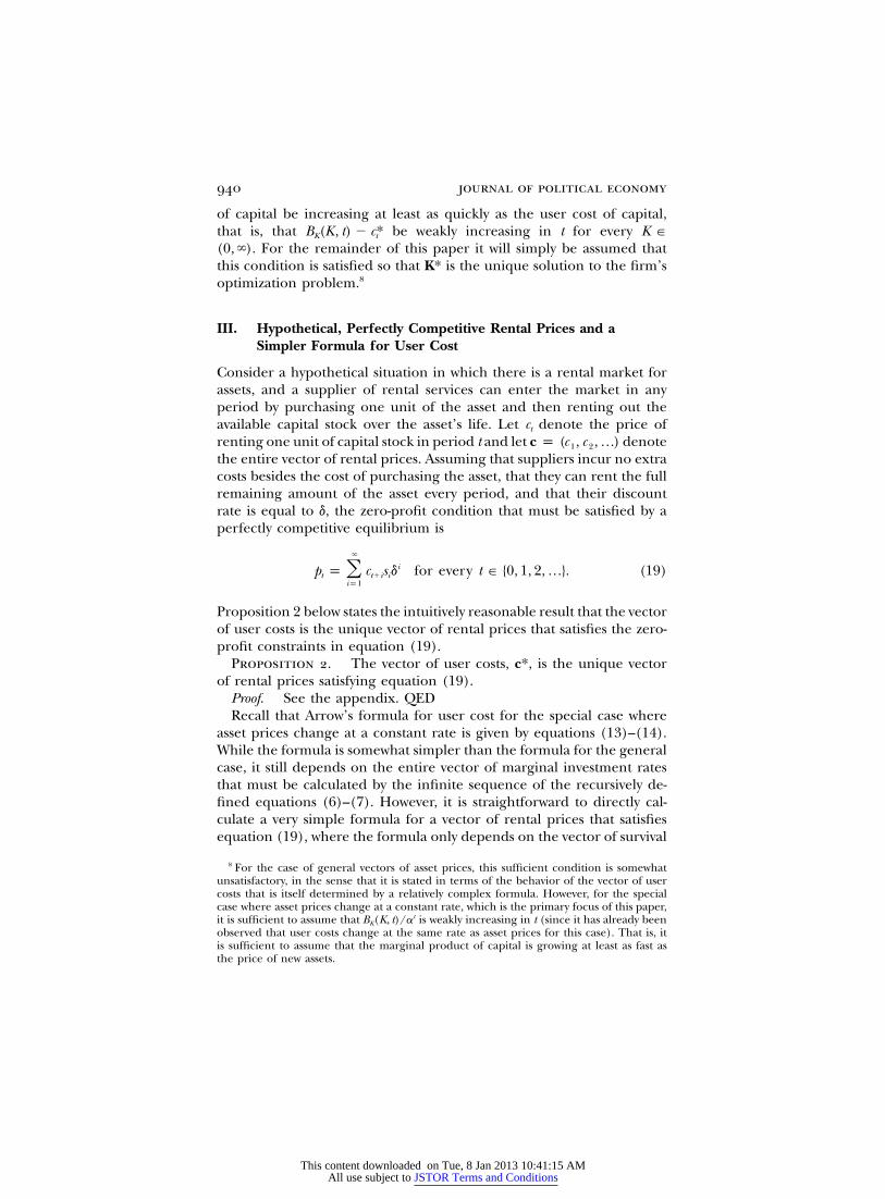
. For the remainder of this paper it will simply be assumed that(0, �)this condition is satisfied so that K* is the unique solution to the firm’soptimization problem.8

III. Hypothetical, Perfectly Competitive Rental Prices and aSimpler Formula for User Cost

Consider a hypothetical situation in which there is a rental market forassets, and a supplier of rental services can enter the market in anyperiod by purchasing one unit of the asset and then renting out theavailable capital stock over the asset’s life. Let ct denote the price ofrenting one unit of capital stock in period t and let denotec p (c , c , …)1 2

the entire vector of rental prices. Assuming that suppliers incur no extracosts besides the cost of purchasing the asset, that they can rent the fullremaining amount of the asset every period, and that their discountrate is equal to d, the zero-profit condition that must be satisfied by aperfectly competitive equilibrium is

�

ip p c s d for every t � {0, 1, 2, …}. (19)�t t�i iip1

Proposition 2 below states the intuitively reasonable result that the vectorof user costs is the unique vector of rental prices that satisfies the zero-profit constraints in equation (19).

Proposition 2. The vector of user costs, c*, is the unique vectorof rental prices satisfying equation (19).

Proof. See the appendix. QEDRecall that Arrow’s formula for user cost for the special case where

asset prices change at a constant rate is given by equations (13)–(14).While the formula is somewhat simpler than the formula for the generalcase, it still depends on the entire vector of marginal investment ratesthat must be calculated by the infinite sequence of the recursively de-fined equations (6)–(7). However, it is straightforward to directly cal-culate a very simple formula for a vector of rental prices that satisfiesequation (19), where the formula only depends on the vector of survival

8 For the case of general vectors of asset prices, this sufficient condition is somewhatunsatisfactory, in the sense that it is stated in terms of the behavior of the vector of usercosts that is itself determined by a relatively complex formula. However, for the specialcase where asset prices change at a constant rate, which is the primary focus of this paper,it is sufficient to assume that is weakly increasing in t (since it has already beentB (K, t)/aK

observed that user costs change at the same rate as asset prices for this case). That is, itis sufficient to assume that the marginal product of capital is growing at least as fast asthe price of new assets.




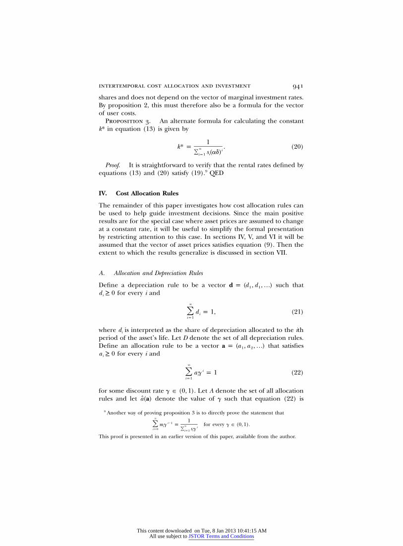
shares and does not depend on the vector of marginal investment rates.By proposition 2, this must therefore also be a formula for the vectorof user costs.

Proposition 3. An alternate formula for calculating the constantk* in equation (13) is given by

1k* p . (20)� i� s(ad)iip1

Proof. It is straightforward to verify that the rental rates defined byequations (13) and (20) satisfy (19).9 QED

IV. Cost Allocation Rules

The remainder of this paper investigates how cost allocation rules canbe used to help guide investment decisions. Since the main positiveresults are for the special case where asset prices are assumed to changeat a constant rate, it will be useful to simplify the formal presentationby restricting attention to this case. In sections IV, V, and VI it will beassumed that the vector of asset prices satisfies equation (9). Then theextent to which the results generalize is discussed in section VII.

A. Allocation and Depreciation Rules

Define a depreciation rule to be a vector such thatd p (d , d , …)1 1

for every i andd ≥ 0i

�

d p 1, (21)� iip1

where di is interpreted as the share of depreciation allocated to the ithperiod of the asset’s life. Let D denote the set of all depreciation rules.Define an allocation rule to be a vector that satisfiesa p (a , a , …)1 2

for every i anda ≥ 0i

�

ia g p 1 (22)� iip1

for some discount rate . Let A denote the set of all allocationg � (0, 1)rules and let denote the value of g such that equation (22) isa(a)

9 Another way of proving proposition 3 is to directly prove the statement that� 1i�1m g p for every g � (0, 1).� i � i

ip0 � s giip1

This proof is presented in an earlier version of this paper, available from the author.




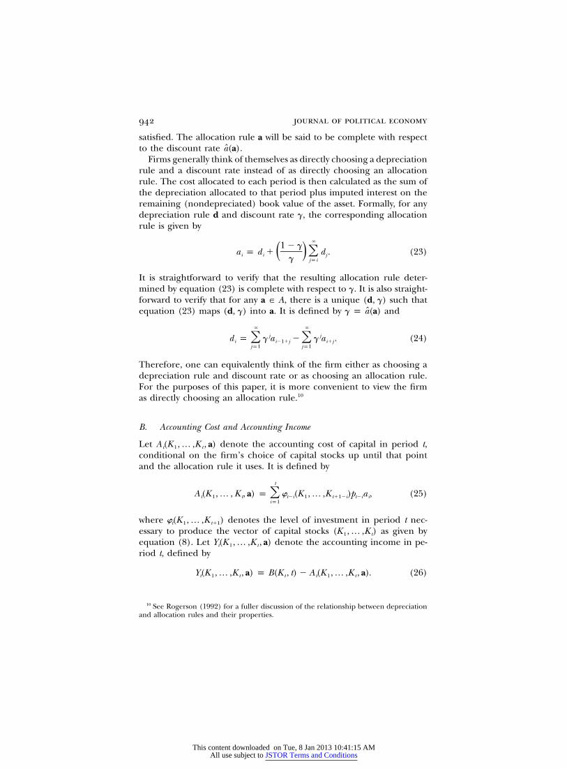
satisfied. The allocation rule a will be said to be complete with respectto the discount rate .a(a)

Firms generally think of themselves as directly choosing a depreciationrule and a discount rate instead of as directly choosing an allocationrule. The cost allocated to each period is then calculated as the sum ofthe depreciation allocated to that period plus imputed interest on theremaining (nondepreciated) book value of the asset. Formally, for anydepreciation rule d and discount rate g, the corresponding allocationrule is given by

�1 � ga p d � d . (23)�i i j( )g jpi

It is straightforward to verify that the resulting allocation rule deter-mined by equation (23) is complete with respect to g. It is also straight-forward to verify that for any , there is a unique (d, g) such thata � Aequation (23) maps (d, g) into a. It is defined by andˆg p a(a)

� �

j jd p g a � g a . (24)� �i i�1�j i�jjp1 jp1

Therefore, one can equivalently think of the firm either as choosing adepreciation rule and discount rate or as choosing an allocation rule.For the purposes of this paper, it is more convenient to view the firmas directly choosing an allocation rule.10

B. Accounting Cost and Accounting Income

Let denote the accounting cost of capital in period t,A (K , … ,K , a)t 1 t

conditional on the firm’s choice of capital stocks up until that pointand the allocation rule it uses. It is defined by

t

A (K , … , K , a) p J (K , … ,K )p a , (25)�t 1 t t�i 1 t�1�i t�i iip1

where denotes the level of investment in period t nec-J(K , … ,K )t 1 t�1

essary to produce the vector of capital stocks as given by(K , … ,K )1 t

equation (8). Let denote the accounting income in pe-Y(K , … ,K , a)t 1 t

riod t, defined by

Y(K , … ,K , a) p B(K , t) � A (K , … ,K , a). (26)t 1 t t t 1 t

10 See Rogerson (1992) for a fuller discussion of the relationship between depreciationand allocation rules and their properties.




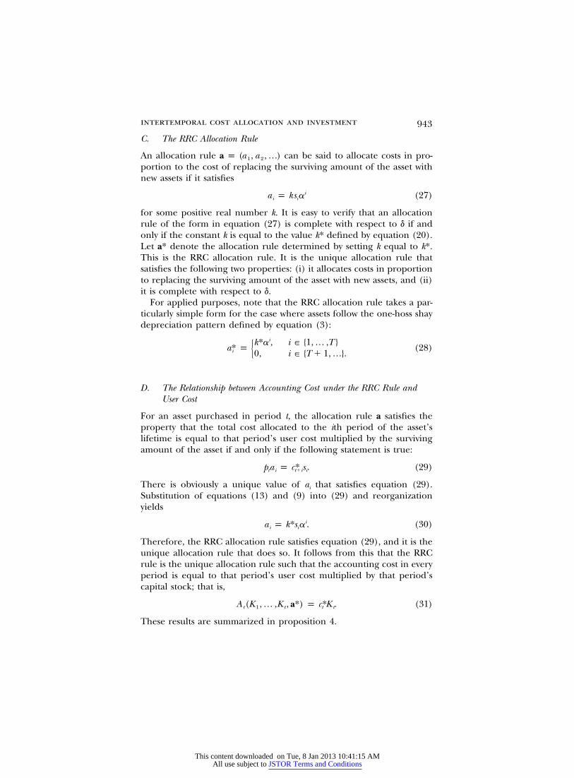
C. The RRC Allocation Rule

An allocation rule can be said to allocate costs in pro-a p (a , a , …)1 2

portion to the cost of replacing the surviving amount of the asset withnew assets if it satisfies

ia p ks a (27)i i

for some positive real number k. It is easy to verify that an allocationrule of the form in equation (27) is complete with respect to d if andonly if the constant k is equal to the value k* defined by equation (20).Let a* denote the allocation rule determined by setting k equal to k*.This is the RRC allocation rule. It is the unique allocation rule thatsatisfies the following two properties: (i) it allocates costs in proportionto replacing the surviving amount of the asset with new assets, and (ii)it is complete with respect to d.

For applied purposes, note that the RRC allocation rule takes a par-ticularly simple form for the case where assets follow the one-hoss shaydepreciation pattern defined by equation (3):

ik*a , i � {1, … ,T }a* p (28)i {0, i � {T � 1, …}.

D. The Relationship between Accounting Cost under the RRC Rule andUser Cost

For an asset purchased in period t, the allocation rule a satisfies theproperty that the total cost allocated to the ith period of the asset’slifetime is equal to that period’s user cost multiplied by the survivingamount of the asset if and only if the following statement is true:

p a p c* s . (29)t i t�i i

There is obviously a unique value of ai that satisfies equation (29).Substitution of equations (13) and (9) into (29) and reorganizationyields

ia p k*s a . (30)i i

Therefore, the RRC allocation rule satisfies equation (29), and it is theunique allocation rule that does so. It follows from this that the RRCrule is the unique allocation rule such that the accounting cost in everyperiod is equal to that period’s user cost multiplied by that period’scapital stock; that is,

A (K , … ,K , a*) p c*K . (31)t 1 t t t

These results are summarized in proposition 4.




Proposition 4. The RRC allocation rule is the unique allocationrule that satisfies equation (29) and is also the unique allocation rulethat satisfies equation (31).

Proof. As above. QED

V. A Simple Rule for Calculating the Optimal Investment Path

Proposition 5 now states that, when the RRC rule is used to calculateaccounting income, the firm can choose the fully optimal vector ofcapital stocks simply by choosing a level of investment each period tomaximize next period’s accounting income.

Proposition 5. Suppose that the firm calculates accounting incomeusing the allocation rule and chooses a level of invest-a p (a , … ,a )1 n

ment every period to maximize the next period’s accounting income.Then a sufficient condition for the firm to choose K* is that a1 be equalto .a*1

Proof. Suppose that the firm is in period t and that it will thereforechoose Kt�1 by its current-period investment decision. By the user costresult, is chosen to maximizeK*t�1

B(K , t � 1) � c* K . (32)t�1 t�1 t�1

Now suppose that the firm chooses Kt�1 to maximize period t�1 ac-counting income. Then, as long as the nonnegativity constraint on in-vestment does not bind, Kt�1 is chosen to maximize

B(K , t � 1) � p a K . (33)t�1 t 1 t�1

By comparing equations (32) and (33), a sufficient condition for thefirm to choose the fully optimal vector of investments is that p a pt 1

. By proposition 4, a necessary and sufficient condition for this isc*t�1

that . QEDa p a*1 1

Of course, the sufficient condition in proposition 5 only specifies thefirst-period allocation share of the allocation rule used by the firm.Therefore, while the RRC allocation rule satisfies this sufficient condi-tion, there are obviously many other allocation rules that also satisfy it.However, the RRC allocation rule is a particularly simple and naturalallocation rule, and it is not clear that it would be possible to identifysome other equally simple and natural allocation rule that sets a1 equalto but sets ai unequal to for other values of i. Furthermore, thea* a*1 i

next section considers a more complex model in which shareholdersdelegate the investment decision to management, accounting incomeis used as a managerial performance measure, and a sufficient condition




for an allocation rule to create good investment incentives is that theallocation share in every period be set according to the RRC allocationrule.

VI. Managerial Investment Incentives

This section considers an extension of the basic model in which share-holders delegate the investment decision to a better-informed managerand shows that there is a sense in which shareholders can create robustincentives for management to choose the fully efficient investment pathby using accounting income calculated using the RRC allocation ruleas a performance measure for management.

Suppose that the production/demand environment is as describedin the previous sections. Assume that shareholders know s and a andcan therefore calculate the RRC allocation rule but that they do notknow the benefit function and therefore do not have sufficientB(K, t)information to calculate the optimal vector of investments. Assume thatthe manager knows all of the functions and parameters in the modeland is therefore able to calculate the optimal vector of investments.Suppose that shareholders delegate the investment decision to the man-ager and that they create a compensation scheme for the manager bychoosing an allocation rule and wage function. The allocation rule isused to calculate each period’s accounting income. The wage functiondetermines the wage the manager receives each period as a function ofcurrent and past periods’ accounting incomes. Assume that the managerhas preferences over vectors of wage payments (with the property thatthe manager weakly prefers a higher wage in any period, holding thewages in all other periods constant) and chooses the sequence of capitalstocks to maximize his or her own utility.

For any given allocation rule, it will generally be the case that thevector of capital stocks that the manager finds it optimal to choose willdepend in complex ways on the particular wage function being usedand the manager’s own preferences over vectors of wage payments,including his or her personal discount rate. This is because it will gen-erally be the case that an allocation rule will create trade-offs betweenincreasing accounting income in different periods, and the manner inwhich the manager weighs these trade-offs will depend on both thewage function and the manager’s own preferences. However, supposethat there was an allocation rule that had the property that there wasa vector of capital stocks that simultaneously maximized the accountingincome in every period. Then as long as each period’s wage was in-creasing in the current and past periods’ accounting income, it wouldobviously be optimal for the manager to choose this vector of capitalstocks. More formally, an allocation rule a� will be said to create robust




incentives for the manager to choose the vector of capital stocks K�, ifa� satisfies

′ ′ ′(K , … , K ) � arg max Y(K , … , K , a ) for every t � {1, 2, …}.1 t t 1 t(K ,…, K )1 t

(34)

Proposition 6 now states the main result of this section, which is thatthe RRC allocation rule creates robust incentives for the manager tochoose the fully optimal vector of capital stocks.

Proposition 6. The RRC allocation rule, a*, creates robust incen-tives for the manager to choose the fully optimal vector of capital stocks,K*.

Proof. Substitution of equation (31) into (26) shows that accountingincome under the RRC rule is given by

Y(K , … , K , a*) p B(K , t) � c*K . (35)t 1 t t t t

Note that accounting income in period t only depends on Kt and thatit is maximized at . This implies that the vector of capital stocksK*t

simultaneously maximizes accounting income for ev-K* p (K*, K*, …)1 2

ery time period. QEDThe above result requires some interpretation. In particular, it does

not formally show that a contract using the RRC allocation rule is theoptimal solution to a completely specified principal agent problem. Itis clear that such a result would be straightforward to prove in a modelin which it was assumed that the only incentive/information problemwas that the manager is better informed than shareholders about someinformation necessary to calculate the fully optimal investment plan.However, there would be no need in such a model to base the manager’swage on any measure of the firm’s performance. This is because onefully optimal contract would be for shareholders to simply pay the man-ager a constant wage each period that is sufficient to induce the managerto accept the job. Then the manager would be (weakly) willing to choosethe profit-maximizing investment plan.

Therefore, in reality, the result of this paper will only be useful insituations where there is some additional incentive problem that re-quires shareholders to base the manager’s wage on some measure ofthe firm’s performance. A natural candidate would be to assume thatthere is a moral hazard problem within each period, that is, that eachperiod the manager can exert unobservable effort that affects the firm’scash flow that period. This would create a multiperiod moral hazardproblem with asymmetric information. The modeling problem this cre-ates is that solutions to such problems are extremely complex, and thenature of the solution generally depends on particular aspects of the




environment (such as the agent’s preferences) that the principal is un-likely to have reliable information about. Thus, it is not clear that suchcontracts would be suitable for use in the real world, where robustnessto small changes in the environment is likely to be important.

In light of these difficulties, the result of this paper can be interpretedas offering a useful alternative approach. In particular, this paper showsthat, by restricting themselves to choosing a compensation scheme inwhich accounting income is calculated using the RRC allocation ruleand in which each period’s wage is a weakly increasing function ofcurrent and past periods’ accounting income, shareholders can guar-antee in a robust way that the investment incentive problem will becompletely solved and still leave themselves considerable degrees offreedom to address remaining incentive issues. For example, by usingaccounting income based on the RRC allocation rule as a performancemeasure, shareholders could thereby guarantee that the investment in-centive problem was completely solved and then use a “trial and error”process over time to identify a wage function that appeared to createthe appropriate level of effort incentives.

Note that in cases where it is possible to calculate a fully optimalcontract, it may well be that the fully optimal contract does not inducethe agent to choose the profit-maximizing level of investment. However,it is precisely these sorts of calculations that are exceedingly complexand that are unlikely to be robust to small changes in the contractingenvironment.

Of course, the question of whether the results of this section can beused to more formally show that a contract using the RRC allocationrule is the optimal solution to a completely specified principal agentproblem is an interesting question for future research. One observationthat may prove helpful in this regard is that proposition 6 can be statedin a somewhat more general form. Namely, it is clear that for any givendiscount rate , the principal can provide the agent with robustg � (0, 1)incentives to choose the sequence of investments that would be first-best for the discount rate g by using the discount rate g to calculateaccounting income under the RRC rule. Therefore, the RRC allocationrule can actually be used to robustly implement the entire continuumof investment strategies, consisting of the set of investment strategiesthat would be first-best for any discount rate .g � (0, 1)

VII. General Patterns of Future Asset Prices

This section reports the extent to which the results of this paper gen-eralize to the case where asset prices do not necessarily change at aconstant rate. In brief, it is still possible to define cost allocation rulesin terms of the vector of user costs so that the resulting cost allocation




rules have the same sorts of desirable properties as were shown to holdin previous sections. The main difference is that there is no longernecessarily any simple or natural way to describe these allocation rulesin terms of the underlying parameters of the model. Therefore, whilethe generalization is of analytic interest because it helps clarify preciselywhy the cost allocation result is true and what it depends on, it may beof more limited practical interest. However, a firm’s information aboutfuture prices is likely to be somewhat imprecise in any event, so that itmay be very natural and reasonable in many applied cases to projectfuture prices by simply specifying a likely average future growth rate.

The remainder of this section provides a very brief sketch of themanner in which the results generalize. For the general case it will benecessary to potentially allow the firm to choose a different allocationrule to allocate each period’s investment. Let denotea p (a , a , …)t t1 t2

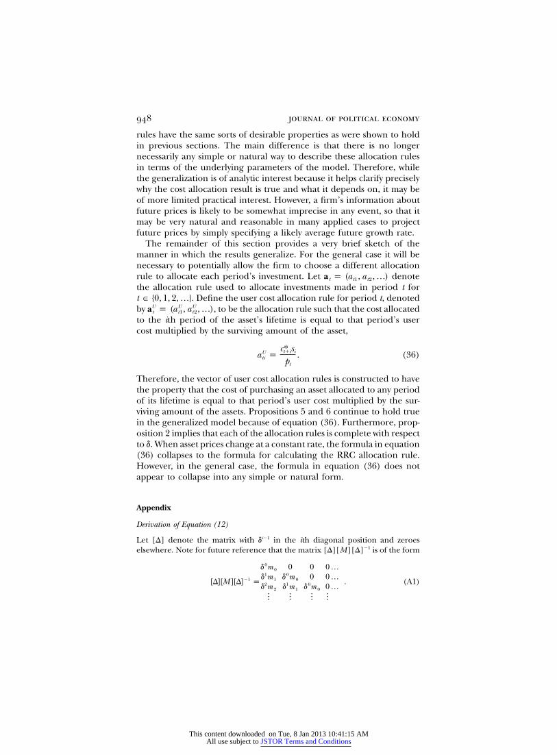
the allocation rule used to allocate investments made in period t for. Define the user cost allocation rule for period t, denotedt � {0, 1, 2, …}

by , to be the allocation rule such that the cost allocatedU U Ua p (a , a , …)t t1 t2

to the ith period of the asset’s lifetime is equal to that period’s usercost multiplied by the surviving amount of the asset,

c* st�i iUa p . (36)ti pt

Therefore, the vector of user cost allocation rules is constructed to havethe property that the cost of purchasing an asset allocated to any periodof its lifetime is equal to that period’s user cost multiplied by the sur-viving amount of the assets. Propositions 5 and 6 continue to hold truein the generalized model because of equation (36). Furthermore, prop-osition 2 implies that each of the allocation rules is complete with respectto d. When asset prices change at a constant rate, the formula in equation(36) collapses to the formula for calculating the RRC allocation rule.However, in the general case, the formula in equation (36) does notappear to collapse into any simple or natural form.

Appendix

Derivation of Equation (12)

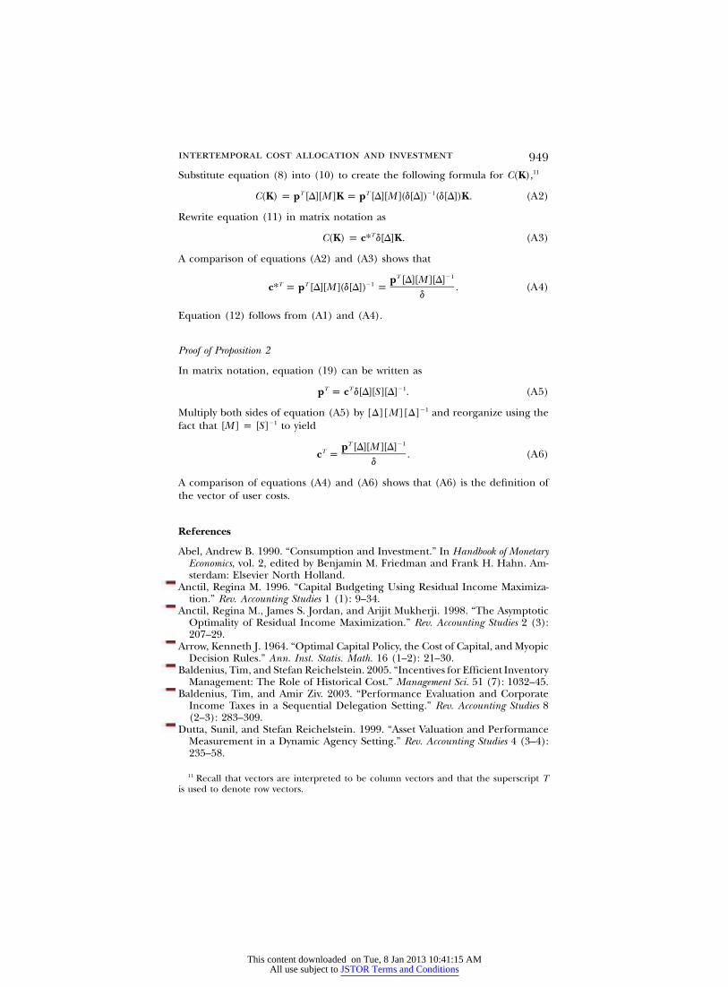
Let [D] denote the matrix with di�1 in the ith diagonal position and zeroeselsewhere. Note for future reference that the matrix [D][M][D]�1 is of the form

0d m 0 0 0 …01 0d m d m 0 0 …�1 1 0[D][M][D] p . (A1)2 1 0d m d m d m 0 …2 1 0

_ _ _ _




Substitute equation (8) into (10) to create the following formula for C(K),11

T T �1C(K) p p [D][M]K p p [D][M](d[D]) (d[D])K. (A2)

Rewrite equation (11) in matrix notation as

TC(K) p c* d[D]K. (A3)

A comparison of equations (A2) and (A3) shows that

T �1p [D][M][D]T T �1c* p p [D][M](d[D]) p . (A4)d

Equation (12) follows from (A1) and (A4).

Proof of Proposition 2

In matrix notation, equation (19) can be written as

T T �1p p c d[D][S][D] . (A5)

Multiply both sides of equation (A5) by [D][M][D]�1 and reorganize using thefact that to yield�1[M] p [S]

T �1p [D][M][D]Tc p . (A6)d

A comparison of equations (A4) and (A6) shows that (A6) is the definition ofthe vector of user costs.

References

Abel, Andrew B. 1990. “Consumption and Investment.” In Handbook of MonetaryEconomics, vol. 2, edited by Benjamin M. Friedman and Frank H. Hahn. Am-sterdam: Elsevier North Holland.

Anctil, Regina M. 1996. “Capital Budgeting Using Residual Income Maximiza-tion.” Rev. Accounting Studies 1 (1): 9–34.

Anctil, Regina M., James S. Jordan, and Arijit Mukherji. 1998. “The AsymptoticOptimality of Residual Income Maximization.” Rev. Accounting Studies 2 (3):207–29.

Arrow, Kenneth J. 1964. “Optimal Capital Policy, the Cost of Capital, and MyopicDecision Rules.” Ann. Inst. Statis. Math. 16 (1–2): 21–30.

Baldenius, Tim, and Stefan Reichelstein. 2005. “Incentives for Efficient InventoryManagement: The Role of Historical Cost.” Management Sci. 51 (7): 1032–45.

Baldenius, Tim, and Amir Ziv. 2003. “Performance Evaluation and CorporateIncome Taxes in a Sequential Delegation Setting.” Rev. Accounting Studies 8(2–3): 283–309.

Dutta, Sunil, and Stefan Reichelstein. 1999. “Asset Valuation and PerformanceMeasurement in a Dynamic Agency Setting.” Rev. Accounting Studies 4 (3–4):235–58.

11 Recall that vectors are interpreted to be column vectors and that the superscript Tis used to denote row vectors.




———. 2002. “Controlling Investment Decisions: Depreciation and CapitalCharges.” Rev. Accounting Studies 7 (2–3): 253–81.

Horngren, Charles T., and George Foster. 1987. Cost Accounting. EnglewoodCliffs, NJ: Prentice Hall.

Jorgensen, Dale W. 1963. “Capital Theory and Investment Behavior.” A.E.R. 53(May): 247–59.

Reichelstein, Stefan. 1997. “Investment Decisions and Managerial PerformanceEvaluation.” Rev. Accounting Studies 2 (2): 157–80.

———. 2000. “Providing Managerial Incentives: Cash Flows versus Accrual Ac-counting.” J. Accounting Res. 38 (2): 243–69.

Rogerson, William P. 1992. “Optimal Depreciation Schedules for Regulated Util-ities.” J. Regulatory Econ. 4 (1): 5–34.

———. 1997. “Intertemporal Cost Allocation and Managerial Investment In-centives.” J.P.E. 105 (4): 770–95.

———. 2008. “On the Relationship between Historic Cost, Forward-LookingCost, and Long Run Marginal Cost.” Manuscript, Dept. Econ., NorthwesternUniv.

Sheehan, Timothy. 1994. “To EVA or Not to EVA: Is That the Question?” Con-tinental Bank J. Appl. Finance 7 (2): 85–87.

Stern, Joel, and Bennett Stewart, moderators. 1994. “Stern Stewart EVA RoundTable.” Continental Bank J. Appl. Finance 7 (2): 46–70.

Stewart, Bennett. 1994. “EVA: Fact and Fantasy.” Continental Bank J. Finance 7(Summer): 71–84.

Tully, Shawn. 1993. “The Real Key to Creating Wealth.” Fortune (September 20):128.



intertemporal cost allocation and investment...

Documents