interval mapping basics

ch. 2 © 2003 Broman, Churchill, Yandell, Zeng 1

2 Key Statistical Issues for QTL• general notation and data structure• recombination model

– two linked markers– flanking markers to a QTL– map distance and map functions

• modelling the phenotype– phenotype model– model likelihood– Bayesian posterior

• missing data concepts and algorithms• model selection


interval mapping basics• observed measurements

– Y = phenotypic trait– X = markers & linkage map

• i = individual index 1,…,n• missing data

– missing marker data– Q = QT genotypes

• alleles QQ, Qq, or qq at locus• unknown genetic architecture

– λ = QT locus (or loci)– θ = genetic action– m = number of QTL

• pr(Q|X,λ,m) recombination model– grounded by linkage map, experimental cross– recombination yields multinomial for Q given X

• pr(Y|Q,θ,m) phenotype model– distribution shape (assumed normal here) – unknown parameters θ (could be non-parametric)

observed X Y

missing Q

unknown λ θafter

Sen Churchill (2001)


2.1 general notation and data structure

• Y = phenotype values– as concept and realized (observed) values

• X = marker genotypes– type of experimental cross– linkage map construction

• marker orders, positions, linkage phases– observed marker genotypes (possibly with error)

• pr(Y,X) = joint probability– what we “know” about Y and X for this experiment– usually assume linkage map is “known”


conditional data likelihood

• condition on markers and linkage map

• pr(X) comprises information on linkage map– not influenced by phenotype– thus can “ignore” for QTL purposes

)(pr),(pr)|(pr

XXYXY =


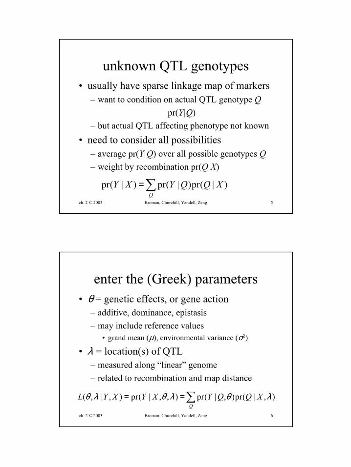
unknown QTL genotypes• usually have sparse linkage map of markers

– want to condition on actual QTL genotype Qpr(Y|Q)

– but actual QTL affecting phenotype not known• need to consider all possibilities

– average pr(Y|Q) over all possible genotypes Q– weight by recombination pr(Q|X)

∑=Q

XQQYXY )|(pr)|(pr)|(pr


enter the (Greek) parameters• θ = genetic effects, or gene action

– additive, dominance, epistasis– may include reference values

• grand mean (µ), environmental variance (σ2)

• λ = location(s) of QTL– measured along “linear” genome– related to recombination and map distance

∑==Q

XQQYXYXYL ),|(pr),|(pr),,|(pr),|,( λθλθλθ


2.2 recombination model• locus λ is distance along linkage map

– identifies flanking marker region• flanking markers provide good approximation

– map assumed known from earlier study– inaccuracy slight using only flanking markers

• extend to next flanking markers if missing data– could consider more complicated relationship

• but little change in results

pr(Q|X,λ) = pr(geno | map, locus) ≈pr(geno | flanking markers, locus)

kX 1+kXQ?

λ


• backcross design– n individuals, 2 markers– follow one gamete

• recombinants– Ab, aB– nR = n12 + n21

• non-recombinants– ab, AB– nNR = n11 + n22

• recombination rate

2.2.1 two linked markersA B

22211211

2112ˆnnnn

nnnnr R

++++==

r

21122211

,,nnnnnn

aBAbABabRNR

RNR +=+=

n21


no linkage?• test for no linkage: r = 1/2• assumption: all individuals have same rate

– implies binomial variation

• normal or chi-square test statisticn

rrrnnnn

nnnnr R )ˆ1(ˆ)ˆ( var,ˆ

22211211

2112 −≈+++

+==

21

22 ~

)/()2/(Zor )1,0(~

)ˆ(var2/1ˆ χ

nnnnnN

rrZ

NRR

R −=−=


binomial probabilitiesbinomial probn = 30,100r = 0.4,0.2

normal approx

knkR rr

kn

kn −−

== )1()(pr


likelihood ratio and LOD test• likelihood for linked markers

• likelihood for unlinked markers

• likelihood ratio and LOD

nCL )()( 21

21 =

22

10

21

2

217.)10log(2

)(log

~)log(2,)ˆ1()ˆ(2

GGLRLOD

LRGrrLR NRR nnn

===

=−= χ

NRR nnR rCrrnnrL )1(),|(pr)( −==


test statistic: distribution

• Z2 and G2 are generally close to each other– Z2 based on properties of counts– G2 and LOD based on likelihood principle– both have approximate chi-square distribution

• (non)central chi-square distribution

22;1

22

21

22

)5.0(4,~,:5.0

~,:5.0

rnncpGZr

GZr

ncp −=<

=

χχ


backcross examples

• n=100 individuals, nR= 40 recombinants– r = 0.4, se(r) = 0.049– Z = -2.04, Z2 = 4.17, p-value = 0.041– G2 = 4.03, LOD = 0.874, p-value = 0.045

• n=100 individuals, nR= 20 recombinants– r = 0.2, se(r) = 0.04– Z = -7.5, Z2 = 56.25, p-value < 0.0001– G2 = 38.55, LOD = 8.37, p-value < 0.0001


backcross examples

• n=30 individuals, nR= 12 recombinants– r = 0.4, se(r) = 0.089– Z = -1.12, Z2 = 1.25, p-value = 0.26– G2 = 1.21, LOD = 0.262, p-value = 0.27

• n=30 individuals, nR= 6 recombinants– r = 0.2, se(r) = 0.073– Z = -4.11, Z2 = 16.87, p-value < 0.0001– G2 = 11.56, LOD = 2.51, p-value < 0.0001


simulations of LOD distribution

n=100,r=0.3,0.51000 sampleshistogram

chi-square curverescaled by 2log(10)

centralr = 0.5

non-centralr = 0.3


LOD and LR over possible rn = 30nR=12 or 6evaluate at

all possible rnot just “best”

LR like a densityLOD is basis for

hypothesis test estimate interval

0.0 0.1 0.2 0.3 0.4 0.5

0.0

e+00

5.0

e-19

1.0

e-18

1.5

e-18

recombination rate

likel

ihoo

d ra

tio

0.0 0.1 0.2 0.3 0.4 0.5

-15

-10

-50

recombination rate

LOD

0.0 0.1 0.2 0.3 0.4 0.5

0.0

e+00

1.0

e-16

2.0

e-16

recombination rate

likel

ihoo

d ra

tio

0.0 0.1 0.2 0.3 0.4 0.5

-4-2

02

recombination rate

LOD


LR, LOD and p-values

p-value p-valueLR LOD 1 d.f. 2 d.f.10 1 0.0319 0.131.6 1.5 0.0086 0.0316100 2 0.0024 0.011000 3 0.0002 0.00110000 4 <0.0001 0.0001


LOD-based interval estimate for rpoint estimate interval estimate

from LOD peakdown 1.5 LOD(or 1 or 2 or …)

n = 30, nR = 12, 6

nnr R /ˆ =

0.20 0.25 0.30 0.35 0.40 0.45 0.50

-1.5

-1.0

-0.5

0.0

n=30,r=0.4

LOD

0.1 0.2 0.3 0.4

0.5

1.0

1.5

2.0

2.5

n=30,r=0.2

LOD


LOD-based interval calculationsconfidence 96.8% 99.1% 99.76%n nR r 1 LOD 1.5 LOD 2 LOD

30 3 0.1 0.03-0.25 0.02-0.29 0.01-0.33100 10 0.1 0.05-0.17 0.04-0.19 0.04-0.2130 6 0.2 0.08-0.37 0.06-0.42 0.05-0.46100 20 0.2 0.13-0.29 0.11-0.31 0.10-0.3330 12 0.4 0.23-0.50 0.19-0.50 0.17-0.50100 40 0.4 0.30-0.50 0.28-0.50 0.26-0.50

Note skew in intervals for small recombination rates.Note upper boundary of 0.5.


LOD-based intervals

0.00 0.10 0.20 0.30

3.0

3.5

4.0

4.5

n=30,r=0.1

LOD

0.1 0.2 0.3 0.4

0.5

1.0

1.5

2.0

2.5

n=30,r=0.2

LOD

0.20 0.30 0.40 0.50

-1.5

-1.0

-0.5

0.0

n=30,r=0.4

LOD

0.05 0.10 0.15 0.20

14.0

14.5

15.0

15.5

16.0

n=100,r=0.1

LOD

0.10 0.15 0.20 0.25 0.30

6.5

7.0

7.5

8.0

n=100,r=0.2

LOD

0.30 0.35 0.40 0.45 0.50

-1.0

-0.5

0.0

0.5

n=100,r=0.4

LOD


likelihood & Bayesian posterior• recall the likelihood and likelihood ratio:

• posterior turns likelihood into a density– assume r may be any value prior to seeing data– posterior = likelihood x prior / constant

NRR

NRR

nnn

nnR

rrrLR

rCrrnnrL

)1(2)(

)1(),|(pr)(

−=

−==

1),|(pr sumcurve or likelihoodunder area

/)(or /)(),|(pr

==

==

Rr

R

nnrLRA

ArLRArLnnr


LR and Bayes posteriorimagine LR as density

area under curve = 1pr(r | nR ) = LR(r) / A

what is probability that ris between 0.25 and 0.5?

where is interval with highest posterior mass? (HPD region)

example: n=30, nR =12,695% HPD regions

0.0 0.1 0.2 0.3 0.4 0.5

0.0

e+00

1.0

e-18

recombination rate

likel

ihoo

d ra

tio

0.0 0.1 0.2 0.3 0.4 0.5

0.00

00.

010

0.02

0

recombination rate

dens

ity

0.0 0.1 0.2 0.3 0.4 0.5

0.0

e+00

1.5

e-16

recombination rate

likel

ihoo

d ra

tio

0.0 0.1 0.2 0.3 0.4 0.5

0.00

00.

010

0.02

0

recombination rate

dens

ity


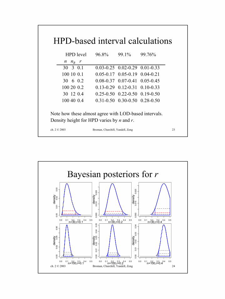
HPD-based interval calculationsHPD level 96.8% 99.1% 99.76%n nR r

30 3 0.1 0.03-0.25 0.02-0.29 0.01-0.33100 10 0.1 0.05-0.17 0.05-0.19 0.04-0.2130 6 0.2 0.08-0.37 0.07-0.41 0.05-0.45100 20 0.2 0.13-0.29 0.12-0.31 0.10-0.3330 12 0.4 0.25-0.50 0.22-0.50 0.19-0.50100 40 0.4 0.31-0.50 0.30-0.50 0.28-0.50

Note how these almost agree with LOD-based intervals.Density height for HPD varies by n and r.


Bayesian posteriors for r

0.0 0.1 0.2 0.3 0.4 0.5

0.00

0.01

0.02

0.03

n=30,r=0.1

dens

ity

0.0 0.1 0.2 0.3 0.4 0.5

0.00

00.

010

0.02

0

n=30,r=0.2

dens

ity

0.0 0.1 0.2 0.3 0.4 0.5

0.00

00.

010

0.02

0

n=30,r=0.4

dens

ity

0.0 0.1 0.2 0.3 0.4 0.5

0.00

0.02

0.04

0.06

n=100,r=0.1

dens

ity

0.0 0.1 0.2 0.3 0.4 0.5

0.00

0.01

0.02

0.03

0.04

0.05

n=100,r=0.2

dens

ity

0.0 0.1 0.2 0.3 0.4 0.5

0.00

0.01

0.02

0.03

0.04

n=100,r=0.4

dens

ity


• Reverend Thomas Bayes (1702-1761)– part-time mathematician– buried in Bunhill Cemetary, Moongate, London– famous paper in 1763 Phil Trans Roy Soc London– was Bayes the first with this idea? (Laplace)

• billiard balls on rectangular table– two balls tossed at random (uniform) on table– where is first ball if the second is to its left (right)?

who was Bayes?

prior pr(θ) = 1likelihood pr(Y | θ)= θY(1- θ)1-Y

posterior pr(θ |Y)= ?

θ

Y=1 Y=0

firstsecond


where is the first ball?

=−=

=

=−=

=

∫ −

0)1(212

)|(pr

21)1()(pr

)(pr)(pr)|(pr)|pr(

1

0

1

YY

Y

dY

YYY

YY

θθ

θ

θθθ

θθθ

prior pr(θ) = 1likelihood pr(Y | θ)= θY(1- θ)1-Y

posterior pr(θ |Y)= ?

θ

Y=1 Y=0

first ball

second ball

0.0 0.2 0.4 0.6 0.8 1.0

0.0

0.5

1.0

1.5

2.0

Y = 1

Y = 0

θ

pr(θ

|Y)

(now throw second ball n times)


what is Bayes theorem?• before and after observing data

– prior: pr(θ) = pr(parameters)– posterior: pr(θ|Y) = pr(parameters|data)

• posterior = likelihood * prior / constant– usual likelihood of parameters given data– normalizing constant pr(Y) depends only on data

• constant often drops out of calculation

)(pr)(pr)|(pr

)(pr),(pr)|(pr

YY

YYY θθθθ ×==


Bayes rule for recombination r

∫=

×=

≤≤≤−=≤≤

−==

2/1

02),|(pr)|(pr

:constant g normalizin)|(pr

)(pr),|(pr),|(pr

:rule Bayes2/10

)(2)pr(: ion recombinat onprior

)1(),|(),|(pr

:likelihood

drrnnnn

nnrrnnnnr

baabbra

rrCrnnrLrnn

RR

R

RR

nnRR

NRR

0.0 0.1 0.2 0.3 0.4 0.5

01

23

45

posterior & prior

rela

tive

frequ

ency n=30

nR=12

0.0 0.1 0.2 0.3 0.4 0.5

01

23

45

posterior & prior

rela

tive

frequ

ency n=30

nR=6


two markers in F2 intercross• two meioses

– follow both gametes– 16 possibilities

• ambiguity with AaBb– 0 or 2 recombinations

• log likelihood ratio:lkjlj

( ))5.0(/)(logsumlog xxxx frfnLR =


two markers in F2 intercross• γ = probability of double recombinant

– for AaBb genotype, haplotype not known– need to “guess” the recombinant fraction of n11 offspring

• γ and r are inter-related– no “closed” solution, need to iterate– guess γ , use to estimate r, improve γ , etc.

[ ]) ˆ(2)(21ˆ

)1(AaBb

aBAbpr

11200221121001

22

2|nnnnnnn

nr

rrr

γ

γ

++++++=

+−=

=


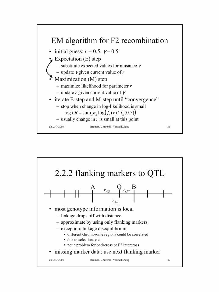
EM algorithm for F2 recombination• initial guess: r = 0.5, γ = 0.5• Expectation (E) step

– substitute expected values for nuisance γ– update γ given current value of r

• Maximization (M) step– maximize likelihood for parameter r– update r given current value of γ

• iterate E-step and M-step until “convergence”– stop when change in log-likelihood is small

– usually change in r is small at this point( ))5.0(/)(logsumlog xxxx frfnLR =


2.2.2 flanking markers to QTL

• most genotype information is local– linkage drops off with distance– approximate by using only flanking markers– exception: linkage disequilibrium

• different chromosome regions could be correlated• due to selection, etc.• not a problem for backcross or F2 intercross

• missing marker data: use next flanking marker

A QrAQBrQB

rAB


backcross QTL & flanking markers1 meiosis8 possible genotypes3 recombination ratessmall distances & rates?

no double crossoversρ = rAQ /rAB

A QrAQBrQB

rAB


F2 QTL & flanking markers2 meioses27 possible genotypes3 recombination ratesEM steps on γ and rABsmall distances & rates?

no double crossovers

A QrAQBrQB

rAB

22

2

)1(,/

ABAB

ABABAQ rr

rrr+−

== γρ


2.2.3 map distance & map functions• How to relate genetic linkage to physical distance?

– math assumptions = crude approximations– critical for map building, minor effect on QTL

• x = genetic map distance (1Morgan = 100cM)– expected number of crossovers per meiosis between

two loci on a single chromatid strand (Sturtevant 1913)

• typical map functions– Morgan: interference rAB = rAQ + rQB

– Kosambi: intermediate rAB = (rAQ + rQB)/(1+4rAQ rQB)– Haldane: no interference rAB = rAQ + rQB - 2rAQ rQB


2.3 modelling the phenotype• trait = mean + genetic + environment• pr( trait Y | genotype Q, effects θ )

EGYGQY

Q

Q

++=

=

µσθ ),(normal),|(pr 2

8 9 10 11 12 13 14 15 16 17 18 19 20

qq QQ

Qq


caution: don’t trust raw histograms!

8 9 10 11 12 13 14 15 16

qqQq

QQ

no QTL?

8 9 10 11 12 13 14 15 16

qqQq

QQ

skewed?

8 9 10 11 12 13 14 15 16 17 18 19 20 21

qqQq

QQ

dominance?

0 1 2 3 4 5 6 7 8 9

qq

QqQQ

zeros?


2.3.1 phenotype model• how is phenotype related to genotype?• typical assumptions

– normal environmental variation• residuals e (not Y!) have bell-shaped histogram

– genetic value GQ is composite of a few QTL• other polygenic effects same across all individuals

– genetic effect uncorrelated with environment

effects ),,(

),|(var,),|(

),0(~,

2

2

2

σµθ

σθµθ

σµ

Q

Q

Q

G

QYGQYE

NeeGY

=

=+=

++=


F2 intercross phenotype model• here assume only one QTL• genotypes QQ, Qq, qq• genotypic values GQQ, GQq, Gqq

• decompose as additive, dominance effects

222:Cockerham-Fisher:Jinx-Mather

qqQqQQ: genotype

δδδ αµµαµαµδµαµ−−+−+=

−++==

Q

Q

GG

Q


2.3.2 model likelihood• why study the likelihood?

– uncover hidden aspects of QTL– loci λ, effects θ, given data (Y,X)

• what is evidence to support a QTL?• where are the QTL? • how precise can estimate the loci & effects?• what genetic architecture is supported?


building the model likelihood• likelihood links phenotype & recombination

– through unknown QTL genotypes Q– mixture over all possible genotypes

• contribution from individual i

• product over all individuals

),,|(pr prod),|,(

),|(pr),|(prsum prod),|,(

),|(pr),|(pr sum),,|(pr

λθλθλθλθ

λθλθ

iii

iiQi

iiQii

XYXYL

XQQYXYL

XQQYXY

=

=

=


and if there are no QTL?

• Y = µ + e, or L(µ | Y )• no relationship with markers & map X• for normal data, maximum likelihood yields

nYYs

nYYYNYL

ii

ii

/)(sumˆ/sumˆ

),|()|(

222

2

−==

===

•

σµ

σµµ


maximum likelihood & LOD• likelihood peaks at some (θ,λ)

– use “hat” (^) to signify value at maximum• LOD profiles likelihood peak

– find θ to maximize likelihood for each λ– profile (scan) loci λ over entire genome

=

==

)|(max),|,(maxlog),|(

),,|(pr prod),,|(pr),|,(

10 YLXYLXYLOD

XYXYXYL iii

µλθλ

λθλθλθ

µ

θ


2.3.3 Bayesian posterior

• treat unknowns as random– build “uncertainty” into model framework– genetic architecture: gene action θ, QTL locus λ

• interpret weighted likelihood as a density– weights based on prior “beliefs”

)|(pr)(pr)|,(pr)|(pr

)|,(pr),,|(pr),|,(pr

XXXY

XXYXY

λθλθ

λθλθλθ

=

=


choice of Bayesian priors• elicited priors

– higher weight for more probable parameter values• based on prior empirical knowledge

– use previous study to inform current study• weather prediction, previous QTL studies on related organisms

• conjugate priors– convenient mathematical form– essential before computers, helpful now to simply computation– large variances on priors reduces their influence on posterior

• non-informative priors – may have “no” information on unknown parameters– prior with all parameter values equally likely

• may not sum to 1 (improper), which can complicate use• always check sensitivity of posterior to choice of prior


incorporate missing genotypes Q• augment data with missing genotypes Q

– use recombination model to state uncertainty– avoid likelihood mixture by augmentation

• marginal posterior on unknowns of interest– average over fully augmented posterior

),|,,(pr sum),|,(pr)|(pr

)|,(pr),|(pr),|(pr),|,,(pr

XYQXYXY

XXQQYXYQ

Q λθλθ

λθλθλθ

=

=


Bayesian parameter estimates• estimates are posterior means or modes

– mean = weighted average of all possible values– mode = maximum

• can get joint or marginal estimates

( )),|,(pr sum argmaxˆ),|,(pr sumˆ

mode

,mean

XY

XY

λθθ

λθθθ

λθ

λθ

=

=


2.4 missing data concepts

• missing QTL genotype Q--see section 2.3• missing marker data X

– errors in genotyping– difficulty reading signal (on gel)– marker not fully informative

• distinguish full data X from observed Xobs– weighted average over all possible marker values

)|(pr),|(prsum),|(pr obsobs XXXQXQ X λλ =

interval mapping basics

Documents