intra-national versus international trade in the european union: why do national borders matter?

www.elsevier.com/locate/econbase

Journal of International Economics 63 (2004) 93–118

Intra-national versus international trade in the

European Union: why do national borders matter?

Natalie Chena,b,c,*

aDepartment of Economics, London Business School, Regent’s Park, London NW1 4SA, UKbECARES, Universite Libre de Bruxelles, 50 av. Roosevelt, 1050 Brussels, Belgium

cCEPR, 90–98 Goswell Road, London EC1V 7RR, UK

Received 16 May 2002; received in revised form 29 November 2002; accepted 16 December 2002

Abstract

The first objective of this paper is to estimate border effects among European Union countries.

In this context, the specification of the gravity equation, together with the choice of the distance

measure, are shown to be crucial for assessing the size of the border effect. The second objective

is to evaluate the determinants of the cross-commodity variation in national border effects.

Contrary to previous findings reported in the literature, we show that trade barriers do provide an

explanation. In particular, technical barriers to trade, together with product-specific information

costs, increase border effects, whereas non-tariff barriers are not significant. Our results further

suggest that these barriers are not the only cause since the spatial clustering of firms is also found

to matter.

D 2003 Elsevier B.V. All rights reserved.

Keywords: Border effects; Trade; EU countries; Industries; Gravity equation

JEL classification: F14; F15

1. Introduction

A growing literature has documented the negative impact of national borders on the

volume of trade. This strand of research was initiated by McCallum (1995) who, using

Canadian provinces and US states-level data in 1988, shows that trade flows between two

0022-1996/$ - see front matter D 2003 Elsevier B.V. All rights reserved.

doi:10.1016/S0022-1996(03)00042-4

* Tel.: +44-20-7262-5050x3395; fax: +44-20-7402-0718.

E-mail address: [email protected] (N. Chen).

URL: http://www.london.edu/.

N. Chen / Journal of International Economics 63 (2004) 93–11894

Canadian provinces were about 22 times as large as their trade with US states, after

controlling for a number of explanatory factors. Subsequent studies1 have illustrated that

domestic trade volumes usually tend to be five to twenty times larger than international

trade volumes. While it is not surprising that national borders create a barrier to the free

flow of goods, it is the size of the effect that is puzzling.

Recent research on the topic has moved from the simple exploration of border effects to

the examination of their likely causes. First and foremost, national trade barriers (tariffs,

quotas, exchange rate variability, transaction costs, different standards and customs,

regulatory differences, etc.) appear as obvious candidates in causing the volume of

domestic trade to exceed that of international trade since they increase the transaction

costs for shipments crossing borders. However, although this trade barrier explanation is

very attractive, the few papers which attempt to explain border effects by (border related)

trade barriers generally find poor evidence in favour of the hypothesis (Wei, 1996;

Hillberry, 1999; Head and Mayer, 2000).

Using a data set of trade between, and within, the states of the US, Wolf (1997,

2000a,b) shows that border effects also extend to the level of sub-national units,

suggesting the existence of additional reasons for ‘excessive’ local trade. A second

explanation could therefore be that intermediate and final goods producers agglom-

erate in order to avoid trade costs, reducing the need for cross-border trade (Wolf,

1997; Hillberry, 1999; Hillberry and Hummels, 2000). Note that the two explanations

are not mutually exclusive, and it could well be that both contribute to the overall

effect.

Since the causes of border effects remain unclear, one objective of this paper is to re-

examine the various hypotheses underlying the creation of border effects, and in particular

to challenge again the trade barriers explanation. Understanding the causes of border

effects is of particular interest because it would enable a better evaluation of their welfare

implications. If border effects reflect the existence of national trade barriers of some kind,

this would indicate that their welfare consequences may well be significant so that there is

some room for increased market integration through the removal of those barriers. In

contrast, if border effects appear to arise endogenously as a consequence of the optimal

location choices of producers, we would conclude that the welfare implications of border

effects are probably small.

The case of the European Union (EU) is particularly appealing since the countries

within the Union are expected to be highly integrated, and hence should display small

border effects. Focusing on seven countries and 78 industries in 1996, the analysis is

undertaken in two stages. Firstly, we provide some estimates of border effects at three

different levels: the pooled level, the country level and, most interestingly, at industry-

specific levels. We stress that the specification of the gravity equation, together with

the choice of the distance measure, are crucial for evaluating the size of the border

effect.

1 See, among others, Helliwell (1995, 1997, 1998, 2000), Wei (1996), Hillberry (1999, 2001), Evans (1999,

2001), Wolf (1997, 2000a,b), Cyrus (2000), Helliwell and Verdier (2000), Nitsch (2000a,b), Head and Mayer

(2000) and Anderson and van Wincoop (2001).

N. Chen / Journal of International Economics 63 (2004) 93–118 95

Secondly, we investigate the role of various border related trade barriers in explaining

border effects across manufacturing industries. In particular, we rely on some data on the

existence of technical barriers to trade across industries. As far as we know, no previous

study has had the opportunity to exploit such data. Our empirical results point to the

importance of these barriers in contributing to border effects across industries. In contrast,

non-tariff barriers are not significant. Our results also provide some evidence supporting

the role of informal barriers to trade, such as product-specific information costs, in

explaining border effects. However, these trade costs only provide an incomplete

explanation for the presence of border effects since the spatial clustering of firms is also

shown to contribute to the overall effect.

The remainder of the paper proceeds as follows: Section 2 presents the model and

discusses specification issues. Section 3 describes the data and the econometric method-

ology implemented. Section 4 provides some estimates for the size of border effects and

discusses the results. Finally, Section 5 is devoted to examining the relevance of various

elements in explaining border effects across industries. Section 6 concludes.

2. The model

In order to explore the impact of national borders on trade flows, our empirical analysis

is based on a standard gravity model since it is the most robust empirical relationship

known in explaining the variation of bilateral trade flows. At the industry-level, the gravity

model considered here takes the following form:

ln Xij;k ¼ b0 þ b1homeþ b2 ln Yi;k þ b3 ln Yj þ b4adjij

þb5 lnDij þ eij;kð1Þ

where i and j indicate the exporting and importing country, respectively, and k the

industry. Xij;k is the bilateral export flow expressed in common currency, Dij is the

distance between i and j and adjij is a dummy equal to one when two countries i and j

share a common border2. As in Evans (1999), Hillberry (1999) and Nitsch (2000a), Yi;kis the production of exporter i in industry k, while Yj is the importing country’s GDP3.

The parameters to be estimated are denoted by b and eij;k is a Gaussian white noise error

term4.

Since the aim is to compare the relative volumes of intra- versus international trade, the

dependent variable includes both international Xij;k i p jð Þ and domestic Xii;k trade

observations. As in previous studies (Wei, 1996; Nitsch, 2000a; Evans, 1999, 2001; Head

and Mayer, 2000), domestic trade Xii;k for country i is just the difference between its total

2 This variable is given a value of zero in the case of domestic trade, which is similar to Helliwell (1997) but

different from Wei (1996).3 See Evans (2001) and Hillberry (2001) for a discussion about the definition of the exporting country’s

output variable.4 We do not include a common language dummy because the countries considered in this paper do not share

such a characteristic.


output and its total exports to the rest of the world. The key parameter is then b1 , the

coefficient on the home dummy variable which is equal to one for domestic trade ðXii;kÞand to zero for international trade ðXij;kÞ. A positive coefficient suggests a preference for

trading within the country rather than with other countries. The antilog of b1 measures the

size of the border effect.

As in most studies (one exception is Hillberry and Hummels, 2002), this paper suffers

from a lack of information on domestic shipment distances, Dii. This is problematic since

the estimated home coefficient is known to be extremely sensitive to the way domestic

distances are measured5. Here, international and intra-national distances are both com-

puted from the weighted averages of the geographic distances between the major cities of

each region using regional GDP weights, allowing to emphasize the regions which should

be more involved in trade. See Appendix A for details.

Without any evidence on actual shipment distances, arguments about ‘correct’

measures of distances are obviously meaningless6. To check the robustness of our results,

we thus consider two alternative measures of internal distances. The first is based on Wei’s

(1996) method of taking a quarter of the distance to the economic centre of the nearest

trading partner, and the second on Leamer (1997) who suggests to take the radius of a

circle (whose area is the area of the country). International distances are calculated

between the economic centres of each country.

When trade flows are disaggregated at the industry level, the inclusion of distance does

not, however, capture that different goods are subject to different transportation costs.

Since the weight-to-value ratio of shipments provides a significant explanation of freight

rates (Hummels, 1999a,b), both distance and weight-to-value will accordingly be consid-

ered as determinants of bilateral trade. Our weight-to-value measure, wvk , is industry-

specific, but averaged across all country pairs ij7:

wvk ¼P

i

Pj Qij;kP

i

Pj Xij;k

" #ð2Þ

where Qij;k is the weight of bilateral exports Xij;k. Since the freight component of costs is

higher for bulky, high weight-to-value raw materials than for manufactures, we expect to

find a negative relationship between weight-to-value and bilateral trade.

Finally, Anderson and van Wincoop (2001) show that, in equilibrium, bilateral trade

depends on both origin and destination price levels, which are themselves related to the

existence of trade barriers (‘multilateral resistance’). Our specification of the gravity

5 See Wei (1996), Leamer (1997), Nitsch (2000a), Helliwell and Verdier (2000), Helliwell (2000) and Head

and Mayer (2000, 2001) for measuring domestic distances and Nitsch (2000b), Hazledine (2000) and Head and

Mayer (2000, 2001) for international distances.6 Using the 1997 US Commodity Flow Survey, Hillberry and Hummels (2002) find that the actual distances

shipped within US states are much shorter than those computed by different authors.7 We do not consider bilateral weight-to-value because: (a) it cannot be computed when trade is zero or

domestic and (b) Hillberry and Hummels (2000) show that bilateral weight-to-value significantly falls with

distance, suggesting that the commodity composition of trade is sensitive to bilateral trade costs, but also that

weight-to-value is endogenous.


equation could therefore lead to biased estimates since relative prices are ignored. Since

each partner should have a different price for each commodity, we control for those

prices (and for any other regional idiosyncrasies) by including origin and destination

fixed-effects, interacted with industry dummies8.

3. Data sources and methodology

The data come from Eurostat, the Statistical Office of the European Commission. The

value of output, bilateral and total exports for manufacturing industries (in thousand ecus),

together with the weight of exports (in tons), are available at the four-digit Nace rev.19

level. GDPs are also taken from Eurostat.

It would clearly be interesting to estimate border effects through time, but due to data

problems10, our sample is purely cross-sectional for 1996 only. Linking total output with

total exports allows us to compute domestic trade Xii;k for seven countries (France,

Germany, Italy, the UK, Spain, Finland and Portugal) and 78 industries, leading to ð78�7Þ ¼ 546 observations. Bilateral exports between countries and industries represent ð7�6Þ � 78 ¼ 3276 observations. The sample therefore covers a total of 3822 observations.

In our data set, about 5% of bilateral exports are equal to zero (no exports are recorded

either because they actually were zero, or because they fell below a reporting threshold).

There are various alternatives to tackle this problem. The zeroes can simply be eliminated

from the sample and the model estimated by OLS. However, this does not seem

appropriate since these omitted observations contain information about why such low

levels of trade are observed. We therefore follow Eichengreen and Irwin (1993, 1998) and

Boisso and Ferrantino (1997) who express the dependent variable as lnð1þ Xij;kÞ:For highlevels of trade flows, lnð1þ Xij;kÞglnðXij;kÞ and for Xij;k ¼ 0, lnð1þ Xij;kÞ ¼ 0. The model

can then be estimated by a tobit procedure. The tobit coefficients are not direct estimates of

the elasticities, but those at sample means can be recovered by the McDonald and Moffitt

(1980) procedure.

Finally, since exporters’ output Yi;k may be endogenous, we instrumented this variable

by the number of workers, but based on a Hausman specification test, the hypothesis of

exogeneity could not be rejected at standard significance levels. Accordingly, exporters’

output is treated as exogenous.

4. The magnitude of border effects

The estimation of Eq. (1) over the pooled sample allows us to assess the average border

effect value for our seven EU countries and 78 industries. Table 1 reports the elasticities at

8 See Hummels (1999a), Hillberry and Hummels (2002) and Rose and van Wincoop (2001).9 Nace rev.1 is the General Industrial Classification of Economic Activities within the European Union.10 Before 1995, output data at the sectoral level was only collected for undertakings with 20 or more persons

employed. In addition, due to the Single Market, the abolition of customs for intra-EU trade has led to changes in

trade statistics since 1993.

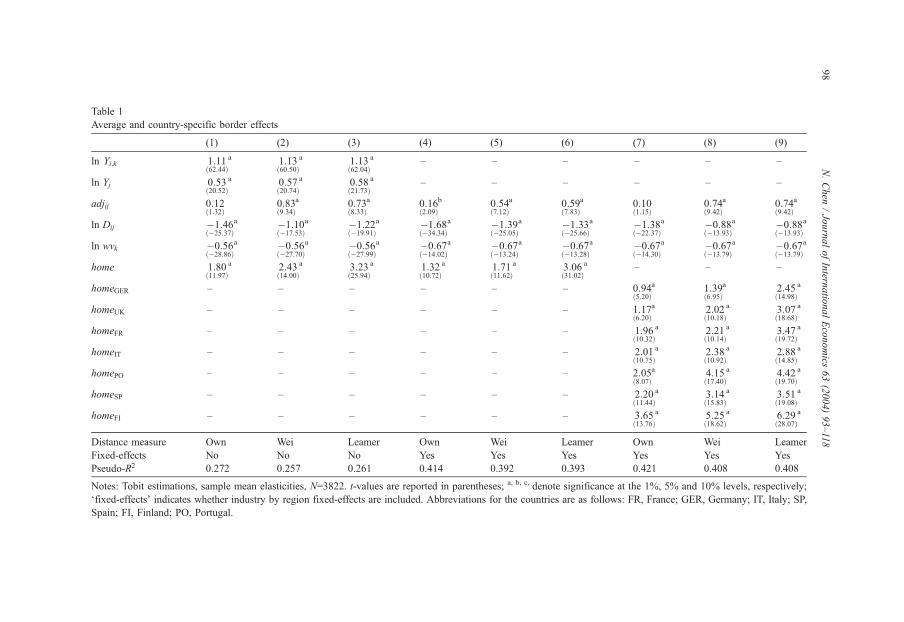
Table 1

Average and country-specific border effects

(1) (2) (3) (4) (5) (6) (7) (8) (9)

ln Yi;k 1:11ð62:44Þ

a 1:13ð60:50Þ

a 1:13ð62:04Þ

a – – – – – –

ln Yj 0:53ð20:52Þ

a 0:57ð20:74Þ

a 0:58ð21:73Þ

a – – – – – –

adjij 0:12ð1:32Þ

0:83ð9:34Þ

a 0:73ð8:33Þ

a 0:16ð2:09Þ

b 0:54ð7:12Þ

a 0:59ð7:83Þ

a 0:10ð1:15Þ

0:74ð9:42Þ

a 0:74ð9:42Þ

a

ln Dij �1:46ð�25:37Þ

a �1:10ð�17:53Þ

a �1:22ð�19:91Þ

a �1:68ð�34:34Þ

a �1:39ð�25:05Þ

a �1:33ð�25:66Þ

a �1:38ð�22:37Þ

a �0:88ð�13:93Þ

a �0:88ð�13:93Þ

a

ln wvk �0:56ð�28:86Þ

a �0:56ð�27:70Þ

a �0:56ð�27:99Þ

a �0:67ð�14:02Þ

a �0:67ð�13:24Þ

a �0:67ð�13:28Þ

a �0:67ð�14:30Þ

a �0:67ð�13:79Þ

a �0:67ð�13:79Þ

a

home 1:80ð11:97Þ

a 2:43ð14:00Þ

a 3:23ð25:94Þ

a 1:32ð10:72Þ

a 1:71ð11:62Þ

a 3:06ð31:02Þ

a – – –

homeGER – – – – – – 0:94ð5:20Þ

a 1:39ð6:95Þ

a 2:45ð14:98Þ

a

homeUK – – – – – – 1:17ð6:20Þ

a 2:02ð10:18Þ

a 3:07ð18:68Þ

a

homeFR – – – – – – 1:96ð10:32Þ

a 2:21ð10:14Þ

a 3:47ð19:72Þ

a

homeIT – – – – – – 2:01ð10:75Þ

a 2:38ð10:92Þ

a 2:88ð14:85Þ

a

homePO – – – – – – 2:05ð8:07Þ

a 4:15ð17:40Þ

a 4:42ð19:70Þ

a

homeSP – – – – – – 2:20ð11:44Þ

a 3:14ð15:83Þ

a 3:51ð19:08Þ

a

homeFI – – – – – – 3:65ð13:76Þ

a 5:25ð18:62Þ

a 6:29ð28:07Þ

a

Distance measure Own Wei Leamer Own Wei Leamer Own Wei Leamer

Fixed-effects No No No Yes Yes Yes Yes Yes Yes

Pseudo-R2 0.272 0.257 0.261 0.414 0.392 0.393 0.421 0.408 0.408

Notes: Tobit estimations, sample mean elasticities, N=3822. t-values are reported in parentheses; a, b, c, denote significance at the 1%, 5% and 10% levels, respectively;

‘fixed-effects’ indicates whether industry by region fixed-effects are included. Abbreviations for the countries are as follows: FR, France; GER, Germany; IT, Italy; SP,

Spain; FI, Finland; PO, Portugal.

N.Chen

/JournalofIntern

atio

nalEconomics

63(2004)93–118

98


sample means calculated by the McDonald and Moffitt (1980) procedure, but the t-

statistics are given for the estimated coefficients.

From the basic gravity equation estimated with our distance measure (column (1)), the

home coefficient is highly significant and equal to 1.80, suggesting that a EU country

trades about six times ½¼ exp 1:80ð Þ�more with itself than with a foreign EU country, after

adjusting for a number of factors. The use of Wei and Leamer distances (columns (2) and

(3)) increases substantially the estimated home coefficient, which therefore appears to be

extremely sensitive to the way distances are measured.

In columns (4) to (6), origin and destination fixed-effects across industries are then

included in order to control for omitted relative prices (note that their inclusion precludes

from the estimation of exporter output and importer income coefficients). In all three

regressions (which use alternative distance measures), the economic impact of crossing the

border is greatly reduced. This finding lends support to the results obtained by Anderson

and van Wincoop (2001) in that omitting relative prices leads to over-estimate the border

effect. See also Hillberry and Hummels (2002).

In all specifications, the basic ‘gravity’ explanatory variables are highly significant and

display coefficients with the expected signs (except for adjacency in column (1)). Weight-

to-value displays a negative and highly significant coefficient, suggesting, as expected,

that a high weight-to-value decreases bilateral trade. In column (4), the coefficient on our

distance measure (equal to �1.68) is larger than the one on Wei (�1.39) or Leamer

(�1.33) distances, but all three coefficients are larger than those reported in many studies

(usually �0.6). Some authors argue that a distance coefficient close to unity (in absolute

value) is far too large to be explained (Hazledine, 2000; Grossman, 1998). Theory

however shows that the elasticity of trade with respect to distance is given by the elasticity

of substitution between products times the elasticity of trade costs with respect to distance

(Anderson and van Wincoop, 2001). As a result, arguing that the coefficient is too large or

too small is obviously not possible without knowing the values of the two factors.

We now turn to the analysis of border effects across countries. To do so, the home

dummy is replaced by country-specific home dummies so that seven home coefficients are

now estimated. The results are reported in the three last columns of Table 1, whose

specifications differ only in terms of the distance measure used.

When using our distances (column (7)), Germany and the UK display the smallest home

coefficients (0.94 and 1.17, respectively). These two countries are followed by France

(1.96), Italy (2.01), Portugal (2.05), Spain (2.20) and finally Finland (3.65). In columns (8)

and (9), where Wei and Leamer distances are used, all home coefficients are larger, but the

ranking of countries remains very similar: Germany always displays the smallest and

Finland the largest home coefficient. The choice of the distance measure therefore affects

the size of the home coefficients, but not necessarily the ranking of countries.

The late accessions of Spain, Portugal (in 1986) and Finland (in 1995) to the EU may

be a possible reason for their larger border effects and hence for their apparent lower

degree of market integration. However, country size seems to matter since the smallest

countries such as Finland or Portugal display the largest effects. This is consistent with

Anderson and van Wincoop (2001) who argue that smaller countries should display larger

border effects because a small drop in international trade can lead to a much larger increase

in trade within a small country than within a large one.


Border effects also differ across industries. Table 2 reports the results of estimating

industry-specific gravity equations. Weight-to-value is now omitted (since its variation is

soaked out by the intercepts), but exporting and importing country fixed-effects are

included. Sectors are ordered in terms of decreasing magnitude of border effects. The

coefficients on distance and adjacency (not reported) are not systematically significant.

However, when they are, the coefficients usually display the expected signs.

When using our distances (column (1)), the largest home coefficient, which is equal to

19.17, is found for ready-mix concrete. It should be noted that among the 42 bilateral trade

observations ipjð Þ included in the sample for that industry, positive trade flows are

recorded in 11 cases only (column (4)), reflecting the domestic orientation of that industry.

The geographic market for ready-mix concrete is, indeed, very local, since the perishable

nature of such a ‘wet’ product constrains the distance over which it can be delivered.

Ready-mix concrete is also the less transportable product of the sample with a weight-to-

value of 35 kilos per ecu (column (5))11.

Large home coefficients are found in many other cases: 5.52 for carpentry and joinery,

4.19 for mortars, 3.76 for printing, 3.27 for metal structures and 3.06 for corrugated paper.

At the opposite end of the spectrum, border effects are not significantly different from zero

in a number of industries such as oils and fats or games and toys. Finally, in the case of

aluminium, the negative and significant (at the 10% level) coefficient on the home variable

suggests a preference for trading with other countries rather than with itself.

Table 2 also reports the industry-specific home coefficients estimated when using Wei

or Leamer distances (columns (2) and (3)). Consistent with our previous findings, ready-

mix concrete always displays the largest coefficient. Also, the coefficients obtained with

Wei or Leamer distances are in general larger than our coefficients. But most importantly,

the ranking of the various industries remains very similar: the correlation between our

coefficients and those obtained with Wei’s distances is equal to 0.98, and to 0.93 with

those obtained with Leamer’s distances. Those findings highlight that the choice of the

distance measure affects the magnitude of the estimates, while the ranking across

industries remains similar12.

The main findings of this section are as follows. Firstly, controlling for relative prices

reduces the size of border effects. Secondly, the way distances are computed affects the

size of border effects, while their ranking across countries or industries remains similar.

5. Explaining border effects

Our results show that border effects vary across industries. We now analyse the factors

which may explain these industry-specific border effects.

11 Note that in 1994, the European concrete industry was taken to the European Court of Justice because of

collusion practices, so the excessively large border effect found for concrete probably also captures the

organization of the industry at that time.12 When excluding ready-mix concrete, which is clearly an outlier in the sample, the correlation between our

coefficients and those obtained with Wei’s distances is equal to 0.94, and to 0.76 with those obtained with

Leamer’s distances.

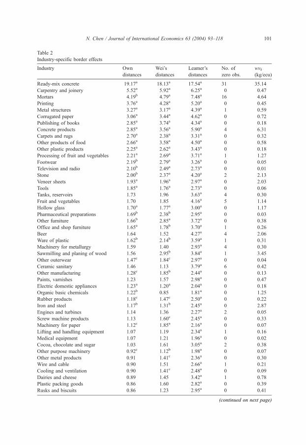
Table 2

Industry-specific border effects

Industry Own Wei’s Leamer’s No. of wvkdistances distances distances zero obs. (kg/ecu)

Ready-mix concrete 19.17a 18.13a 17.54a 31 35.14

Carpentry and joinery 5.52a 5.92a 6.25a 0 0.47

Mortars 4.19b 4.79a 7.48a 16 4.64

Printing 3.76a 4.28a 5.20a 0 0.45

Metal structures 3.27a 3.17a 4.39a 1 0.59

Corrugated paper 3.06a 3.44a 4.62a 0 0.72

Publishing of books 2.85a 3.74a 4.34a 0 0.18

Concrete products 2.85a 3.56a 5.90a 4 6.31

Carpets and rugs 2.70a 2.38a 3.31a 0 0.32

Other products of food 2.66a 3.58a 4.50a 0 0.58

Other plastic products 2.25a 2.62a 3.43a 0 0.18

Processing of fruit and vegetables 2.21a 2.69a 3.71a 1 1.27

Footwear 2.19b 2.79a 3.26a 0 0.05

Television and radio 2.10b 2.49a 2.73a 0 0.01

Stone 2.00b 2.37a 4.20a 2 2.13

Veneer sheets 1.93a 1.96a 2.97a 0 2.03

Tools 1.85a 1.76a 2.73a 0 0.06

Tanks, reservoirs 1.73 1.96 3.63a 4 0.30

Fruit and vegetables 1.70 1.85 4.16a 5 1.14

Hollow glass 1.70a 1.77a 3.00a 0 1.17

Pharmaceutical preparations 1.69b 2.38b 2.95a 0 0.03

Other furniture 1.66b 2.85a 3.72a 0 0.38

Office and shop furniture 1.65a 1.78b 3.70a 1 0.26

Beer 1.64 1.52 4.27a 4 2.06

Ware of plastic 1.62b 2.14b 3.59a 1 0.31

Machinery for metallurgy 1.59 1.40 2.93a 4 0.30

Sawmilling and planing of wood 1.56 2.95b 3.84a 1 3.45

Other outerwear 1.47c 1.84c 2.97a 0 0.04

Ceramic sanitary 1.46 1.13 3.79a 6 0.42

Other manufacturing 1.28c 1.85b 2.44a 0 0.13

Paints, varnishes 1.23 1.57 2.98a 0 0.47

Electric domestic appliances 1.23a 1.20a 2.04a 0 0.18

Organic basic chemicals 1.22b 0.85 1.81a 0 1.25

Rubber products 1.18c 1.47c 2.50a 0 0.22

Iron and steel 1.17b 1.31b 2.45a 0 2.87

Engines and turbines 1.14 1.36 2.27a 2 0.05

Screw machine products 1.13 1.60c 2.45a 0 0.33

Machinery for paper 1.12c 1.85a 2.16a 0 0.07

Lifting and handling equipment 1.07 1.19 2.34a 1 0.16

Medical equipment 1.07 1.21 1.96a 0 0.02

Cocoa, chocolate and sugar 1.03 1.61 3.05a 2 0.38

Other purpose machinery 0.92c 1.12b 1.98a 0 0.07

Other metal products 0.91 1.41c 2.36a 0 0.30

Wire and cable 0.90 1.51 2.66a 1 0.21

Cooling and ventilation 0.90 1.41c 2.48a 0 0.09

Dairies and cheese 0.89 1.45 3.42a 1 0.78

Plastic packing goods 0.86 1.60 2.82a 0 0.39

Rusks and biscuits 0.86 1.23 2.95a 0 0.41

(continued on next page)


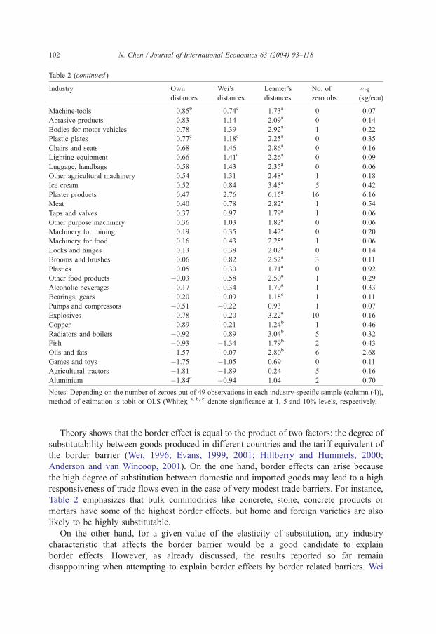
Table 2 (continued )

Industry Own Wei’s Leamer’s No. of wvkdistances distances distances zero obs. (kg/ecu)

Machine-tools 0.85b 0.74c 1.73a 0 0.07

Abrasive products 0.83 1.14 2.09a 0 0.14

Bodies for motor vehicles 0.78 1.39 2.92a 1 0.22

Plastic plates 0.77c 1.18c 2.25a 0 0.35

Chairs and seats 0.68 1.46 2.86a 0 0.16

Lighting equipment 0.66 1.41c 2.26a 0 0.09

Luggage, handbags 0.58 1.43 2.35a 0 0.06

Other agricultural machinery 0.54 1.31 2.48a 1 0.18

Ice cream 0.52 0.84 3.45a 5 0.42

Plaster products 0.47 2.76 6.15a 16 6.16

Meat 0.40 0.78 2.82a 1 0.54

Taps and valves 0.37 0.97 1.79a 1 0.06

Other purpose machinery 0.36 1.03 1.82a 0 0.06

Machinery for mining 0.19 0.35 1.42a 0 0.20

Machinery for food 0.16 0.43 2.25a 1 0.06

Locks and hinges 0.13 0.38 2.02a 0 0.14

Brooms and brushes 0.06 0.82 2.52a 3 0.11

Plastics 0.05 0.30 1.71a 0 0.92

Other food products �0.03 0.58 2.50a 1 0.29

Alcoholic beverages �0.17 �0.34 1.79a 1 0.33

Bearings, gears �0.20 �0.09 1.18c 1 0.11

Pumps and compressors �0.51 �0.22 0.93 1 0.07

Explosives �0.78 0.20 3.22a 10 0.16

Copper �0.89 �0.21 1.24b 1 0.46

Radiators and boilers �0.92 0.89 3.04b 5 0.32

Fish �0.93 �1.34 1.79b 2 0.43

Oils and fats �1.57 �0.07 2.80b 6 2.68

Games and toys �1.75 �1.05 0.69 0 0.11

Agricultural tractors �1.81 �1.89 0.24 5 0.16

Aluminium �1.84c �0.94 1.04 2 0.70

Notes: Depending on the number of zeroes out of 49 observations in each industry-specific sample (column (4)),

method of estimation is tobit or OLS (White); a, b, c, denote significance at 1, 5 and 10% levels, respectively.


Theory shows that the border effect is equal to the product of two factors: the degree of

substitutability between goods produced in different countries and the tariff equivalent of

the border barrier (Wei, 1996; Evans, 1999, 2001; Hillberry and Hummels, 2000;

Anderson and van Wincoop, 2001). On the one hand, border effects can arise because

the high degree of substitution between domestic and imported goods may lead to a high

responsiveness of trade flows even in the case of very modest trade barriers. For instance,

Table 2 emphasizes that bulk commodities like concrete, stone, concrete products or

mortars have some of the highest border effects, but home and foreign varieties are also

likely to be highly substitutable.

On the other hand, for a given value of the elasticity of substitution, any industry

characteristic that affects the border barrier would be a good candidate to explain

border effects. However, as already discussed, the results reported so far remain

disappointing when attempting to explain border effects by border related barriers. Wei


(1996) examines whether the impact of borders can be attributed to exchange rate

volatility between OECD countries, but finds no significant effect. Head and Mayer

(2000) show that non-tariff barriers do not explain border effects in Europe. Using the

estimates of commodity-specific border effects for 136 products traded between

Canada and the US in 1993, Hillberry (1999) investigates the role of trade policy

(tariffs), regulations, information and communication costs (captured by the extent of

multinational activity), product-specific information costs, public procurement and

hysteresis in domestic transportation networks, but none of these appears significant

in explaining border effects.

One objective of this section is hence to challenge the border barriers explanation of

border effects. To do so, we analyse the role of technical barriers to trade (TBTs). Note that

the role of TBTs has not been investigated previously. As quoted by Hillberry (1999, p.

35), due to data unavailability, ‘‘[TBT]-related explanations of border effects must be

relegated to anecdotal evidence’’. Non-tariff barriers (NTBs) are also considered. Finally,

the role of product-specific information costs is explored. In particular, if it is more costly

to obtain some information about the quality, or even the existence, of a foreign product as

compared to a domestic product, we would expect this higher cost to reduce the quantities

of foreign goods purchased (Rauch, 1999), and hence to contribute to the existence of

border effects.

An alternative explanation could be that border effects arise endogenously. The

intuition is that in order to avoid trade costs, intermediate and final goods producers

tend to agglomerate, generating endogenous border effects because intermediate goods

trade is essentially local and within borders. Wolf (1997, 2000b) points out that

intermediate goods trade generally covers shorter distances than does final goods trade,

leading him to argue that the clustering of intermediate stages of production might

explain the large coefficients on the home dummy variable. Hillberry (1999) and

Hillberry and Hummels (2000) also show that the spatial clustering of firms magnifies

border effects. Accordingly, the present paper also checks for whether this alternative

explanation for border effects can be validated by the data when focusing on the

European Union case.

We decide to group the various possible explanations for border effects into two broad

categories: technical and non-tariff barriers to trade, together with product-specific

information costs, are defined as ‘trade costs’, whereas the spatial agglomeration of firms

and the elasticity of substitution among varieties are considered as ‘behavioural responses

to trade costs’.

The next four sections are devoted to our analysis. The first section motivates the

choice of trade cost variables in explaining border effects. The second further extends the

analysis by considering behavioural responses to trade cost variables. The main results are

reported in the third section. Finally, some robustness checks are provided in the last

section.

5.1. Trade cost variables

In the context of achieving the free trade objectives of the Single Market

Programme in Europe, the Mutual Recognition Principle (MRP) states that products


manufactured and sold in one EU country should be lawfully accepted for sale in all

other member states. However, member states have the right to restrict intra-EU

imports on the grounds of health, safety, environmental and consumer protection.

These obstacles, known as technical barriers to trade (TBTs), impose some additional

costs on exporters who want to access foreign markets, and could hence contribute to

border effects. Various measures were implemented in order to remove these barriers13,

but in 1996, about 79% of intra-EU goods trade were still affected by TBTs (European

Commission, 1998).

In order to investigate whether TBTs have an impact on border effects, we rely on

a study undertaken for the European Commission (European Commission, 1998)

which identifies the industries affected by TBTs and assesses, on a five-point scale,

the effectiveness of different measures undertaken: (1) no solution has been adopted,

(2) measures are proposed or implemented, but not effective or with operating

problems, (3) measures are adopted, but with implementation or transitional problems

still to be overcome, (4) measures are implemented and function well, but some

barriers remain, and (5) measures are successful and all significant barriers are

removed. The study also identifies some industries which, prior to European

integration, were not affected by TBTs. This information allows us to compute, for

the sample of industries affected by TBTs, an industry-specific qualitative variable,

tbtk, taking values between one and five with a larger value indicating an increase in

market integration due to removed TBTs.

The choice of this variable might be criticized on the grounds that it captures

changes in border costs rather than levels. For instance, it could be that TBTs were

decreased in an industry k (so that tbtk is equal to four), but that the level of TBTs

continues to be higher than in other industries where no solution was adopted (and

where tbtk is equal to one). Then, tbtk would obviously provide some biased information

about the level of TBTs. To address this issue, we compute a second variable, tbtk*,

which is a dummy equal to one when: (a) industry k was not affected by TBTs prior to

European integration and (b) the measures implemented were successful and all barriers

are removed (that is, when tbtk is equal to five), and zero otherwise. In other words,

tbtk* distinguishes the industries with no TBTs (either because TBTs do not occur or

were eliminated) from those where some barriers persist (whatever the level of those

barriers).

We expect those industries with no TBTs, or with TBTs removed, to display smaller

border effects. In the case of ready-mix concrete, the value of 2 for tbtk , which

indicates that this industry continues to be affected by TBTs, may provide an

explanation for some of its large border effect, with the opposite holding true for

games and toys which are given a value of 5. In addition, locks and hinges and brooms

and brushes, which do not display any border effect, are some of the industries where

TBTs do not occur.

Next, we consider a measure reflecting the importance of non-tariff barriers (NTBs)

across industries. The intuition is that if goods are required to meet certain standards, these

13 The ‘Old Approach’ and ‘New Approach’ to technical harmonisation in particular. See European

Commission (1998) for details.


may act as a tariff or a quota in reducing or even eliminating foreign competition for

domestic producers, so that industries subject to non-tariff barriers are expected to display

larger border effects. The extent to which a sector k is affected by non-tariff barriers is

captured by a qualitative variable ntbk which ranges between 1 and 3 (European

Commission (1997))14. For instance, the extent of non-tariff barriers for television and

radio or pharmaceutical preparations (ntbk equals 3) could be a possible reason for their

large border effects.

It is worth noting that the non-availability of cross-country indicators on NTBs or TBTs

is clearly a shortcoming of this empirical study. Despite the EU integration process, cross-

country differences in NTBs or TBTs continue to exist, and should therefore be considered

in explaining border effects.

Finally, it can be expected that product-specific information costs may also play a

role in explaining border effects. In particular, cost differences to obtain information

about the existence or quality of foreign products may represent informal barriers to

trade. In this context, Rauch (1999) stresses the role of ‘search costs’ as a barrier to

trade for differentiated products by providing evidence that much international exchange

in differentiated products takes place across networks of trading contacts, the extent of

which is determined in part by search-reducing proximity, common language and

common understanding of legal and cultural institutions. We therefore make use of

Rauch’s (1999) US four-digit SITC Rev.2 categorisation of industries according to three

possible types: homogeneous goods (products traded on ‘organised exchange’ markets),

reference priced (products quoted in trade publications) and differentiated products15.

According to Rauch (1999), we would expect that ‘search costs’ are higher for

differentiated products and, therefore, contribute to larger border effects. To check this

assumption, three dummy variables (n for differentiated products, r for reference priced

and w for homogeneous goods) are computed, each characterizing the three industry

types. If Rauch’s (1999) hypothesis is correct, we would expect border effects to be

larger in n-type industries, smaller in r-type ones, and finally to be the smallest for w-

type industries.

5.2. Behavioural responses to trade cost variables

The clustering of firms may provide an additional explanation for the existence of

border effects. In order to investigate this hypothesis, Hillberry (1999) uses an index of

‘geographic concentration’ computed by Ellison and Glaeser (1997) for US industries

at the four-digit SIC level. The index measures the extent to which firms’ production is

tied to any particular geographic location (because firms require natural resources or

benefit from agglomeration externalities). A low value for the index indicates that the

industry in question is not reliant on a specific geographic location, whereas industries

15 This is available at http://www.macalester.edu/research/economics/PAGE/HAVEMAN/Trade.Resources/

TradeData.html#Rauch. Note that Rauch provides two classifications, ‘conservative’ and ‘liberal’.

14 This non-tariff barriers variable captures differences in standards, national preference in public purchases

and customs formalities. In contrast, TBTs essentially refer to technical regulations imposed by national

governments for health, safety, environmental and consumer protection.

http:\\www.macalester.edu\research\economics\page\haveman\

http:\\www.macalester.edu\research\economics\page\haveman\


which require to produce in specific locations display high values. If some firms are

not attached to any specific location (a low value for the index), it can be expected

that they will choose their location of production so as to minimise cross-border

transaction costs, and as a result, border effects could be magnified. The size of the

border effect is therefore expected to be inversely related to the Ellison and Glaeser

(1997) index.

To check for this possibility, the industry-specific indices reported in the unpublished

appendix of Ellison and Glaeser (1994) are matched with our European industries. We

believe that their data, though measured with US data, can provide some information about

the distribution of European industries. For instance, if the US wine industry is highly

dependent on specific locations due to the natural advantages of some regions in growing

grapes, the European wine industry is naturally expected to share the same features. Of

course, it would be better to exploit European data, but the computation of such indices is

well beyond the scope of this paper.

On the whole, the smaller the value of the index (denoted by cok), the more likely the

border effect for the corresponding industry should be larger. For instance, ready-mix

concrete (SIC 3273) displays, in the US, a small index of 0.010, whereas for copper (SIC

3331), the high value of 0.194 suggests that this industry is highly dependent on specific

locations. This pattern of the indices across both US industries could therefore be taken as

prima facie evidence that some of the EU border effects obtained for the corresponding

industries are, to some extent, endogenous.

Finally, the elasticity of substitution among varieties is another potential explanation for

border effects. In order to investigate this possible relationship, the elasticity of substitu-

tion corresponding to each commodity would be required. But as shown by Hummels

(1999a), this elasticity can only be identified when some components of trade costs, such

as tariffs, are directly observable. This is not possible here.

Another way to address this issue is to compare distance coefficients across commod-

ities16. Since those coefficients are given by the elasticity of substitution times the

elasticity of trade costs with respect to distance, we cannot identify the values of the

two factors. Nevertheless, we could expect distance and home coefficients to be highly

(and negatively) correlated if the elasticity of substitution is indeed a large part of the

explanation for border effects. The correlation between home and distance coefficients (not

reported) is however positive and equal to 0.48, suggesting that the elasticity of

substitution is not driving the cross-industry variance in border effects. This is contrary

to Evans (1999) who finds that border effects are largely explained by the elasticity of

substitution across varieties.

5.3. Results

We now examine the relationship between the variables and border effects. To

do so, the gravity equation is estimated over the pooled sample of countries and

industries, including the home variable and an interaction term between home and the

16 We thank an anonymous referee for this suggestion.


explanatory variable of interest (as in Evans, 1999). Since the aim is to compare border

effects across industry types, industry-specific distance interaction terms are included,

together with industry-specific origin and destination fixed-effects ai;k and aj;k . The

specification is17:

lnð1þ Xij;kÞ ¼ ai;k þ aj;k þ c1homeþ c2ðhome� vikÞ þ c3adjij

þPk

ck ln Dij þ eij;kð3Þ

The sign and significance of the c2 coefficient on the interaction term indicates whether

industries with a particular characteristic vik display larger or smaller border effects. In

addition, the magnitude of the home and of the interaction coefficients, c1 and c2 ,permits to assess the relative importance of each explanatory factor vik. In this section,

we only focus on the results obtained with our distance measure.

Is there any evidence that border effects are explained by technical barriers to trade?

The results with the tbtk variable are reported in column (1) of Table 3 (the sample is

restricted to those industries which were affected by TBTs, i.e. N ¼ 3185). The negative

and significant coefficient on the interaction term with tbtk shows that industries where

TBTs were removed display smaller border effects. The coefficients on home (3.80) and on

the interaction term (�0.67) further indicate that industries where TBTs are eliminated

tbtk ¼ 5ð Þhave a home coefficient of 3:80� 0:67� 5ð Þð Þ ¼ 0:45, whereas on the contrary,industries where no solution was adopted tbtk ¼ 1ð Þ have a coefficient of

3:80� 0:67� 1ð Þð Þ ¼ 3:13 . For the other intermediate industries, which are given a

value of 2, 3 and 4 for tbtk , home coefficients lie between 0.45 and 3.13. The results

suggest that deeper market integration, in the form of reduced TBTs, reduces the impact of

borders on trade flows.

From column (2), when using the tbtk* measure, we see that industries with no TBTs

(tbtk*¼ 1 ) generally display smaller border effects: their home coefficient is equal to

1:54� 0:60� 1ð Þð Þ ¼ 0:94 against 1:54� 0:60� 0ð Þð Þ ¼ 1:54 for industries where some

barriers remain (that is, all those industries with a tbtk value of 1, 2, 3 and 4). Given that

tbtk and tbtk* yield comparable results, we conclude that tbtk does provide some general

information about the extent of TBTs across industries.

The results on non-tariff barriers are reported in column (3). The positive but

insignificant coefficient on the interaction term implies that non-tariff barriers do not

matter in explaining border effects, a finding consistent with that by Head and Mayer

(2000).

Spatial clustering is explored in column (4). As expected, firms with a small value of

the Ellison and Glaeser (1997) index display larger border effects. This lends support to

the arguments by Wolf (1997, 2000a,b), Hillberry (1999) and Hillberry and Hummels

(2000) in that firms not tied to any specific location probably locate so as to minimise trade

costs. As a result, international trade is reduced and border effects appear endogenously.

17 Note that with industry-specific distance interaction terms, weight-to-value is now omitted because of a

multicollinearity problem (its coefficient changes sign).

Table 3

Explaining border effects (dependent variable is ln 1þ Xij;k

� �, own distance measure)

(1) (2) (3) (4) (5) (6) (7) (8) (9) (10)

adjij 0:19ð2:45Þ

b 0:17ð2:46Þ

b 0:17ð2:45Þ

b 0:17ð2:50Þ

b 0:17ð2:45Þ

b 0:17ð2:45Þ

b 0:17ð2:45Þ

b 0:17ð2:45Þ

b 0:19ð2:49Þ

b 0:17ð2:50Þ

b

ln Dij �1:80ð�26:64Þ

a �1:76ð�27:56Þ

a �1:76ð�27:47Þ

a �1:77ð�28:07Þ

a �1:77ð�27:64Þ

a �1:76ð�27:49Þ

a �1:77ð�27:50Þ

a �1:77ð�27:64Þ

a �1:79ð�26:96Þ

a �1:77ð�28:08Þ

a

home 3:80ð17:50Þ

a 1:54ð13:24Þ

a 1:25ð6:81Þ

a �0:51ð�2:72Þ

a 1:38ð12:41Þ

a 1:26ð11:23Þ

a 1:17ð8:90Þ

a – – –

home� tbtk �0:67ð�14:01Þ

a – – – – – – – �0:70ð�12:26Þ

a –

home� tbtk* – �0:60ð�6:19Þ

a – – – – – – – �0:35ð�3:20Þ

a

home� ntbk – – 0:02ð0:28Þ

– – – – – �0:16ð�1:62Þ

�0:10ð�1:13Þ

home� ln cok – – – �0:45ð�11:72Þ

a – – – – �0:35ð�7:90Þ

a �0:42ð�10:31Þ

a

home� w – – – – �0:60ð�4:38Þ

a – – 0:78ð4:86Þ

a 3:22ð7:81Þ

a �0:16ð�0:53Þ

home� r – – – – – 0:24ð1:87Þ

c – 1:50ð9:78Þ

a 2:89ð7:18Þ

a �0:13ð�0:44Þ

home� n – – – – – – 0:19ð1:79Þ

c 1:36ð11:86Þ

a 2:62ð7:25Þ

a �0:04ð�0:16Þ

N 3185 3822 3822 3822 3822 3822 3822 3822 3185 3822

pseudo-R2 0.46 0.46 0.46 0.46 0.46 0.46 0.46 0.46 0.46 0.46

Notes: Tobit estimations, sample mean elasticities. Industry-specific distance interaction terms (meat is the excluded industry), and industry-specific origin and destination

fixed-effects are included (not reported); t-values are reported in parentheses; a, b, c, denote significance at 1%, 5% and 10% levels, respectively. The probabilities

associated with the hypotheses that w and r effects, r and n effects, and w and n effects, are equal are, respectively, 0.00, 0.27 and 0.00 in column (8), 0.07, 0.07 and 0.00 in

column (9) and 0.88, 0.50 and 0.45 in column (10).

N.Chen

/JournalofIntern

atio

nalEconomics

63(2004)93–118

108


In our sample of industries, the Ellison and Glaeser (1997) index varies between 0.001

for corrugated paper and 0.378 for carpets and rugs. This means that for an industry

with an index of 0.001, the home coefficient would, on average, be equal to

(�0:51� 0:45� ln0:001ð Þ)¼ 2:60 while for an industry with an index of 0.378, the ho

me coefficient would be (�0:51� 0:45� ln0:378ð Þ)¼ �0:07.Columns (5) to (8) show that product-specific information costs are also relevant in

explaining border effects18: from columns (5) to (7), w-type industries display smaller

border effects; in contrast, r- and n-type industries display larger effects. In column (8),

when replacing the aggregate home dummy by one dummy specific to each industry

type, the home coefficients for reference priced r and differentiated products n ,

respectively equal to 1.50 and to 1.36, are both significantly larger than the one for w-

type industries (equal to 0.78): the probability associated with the hypotheses that the

coefficients on w- and r-type industries, and on w- and n-type industries, are equal is

equal to zero, but we cannot reject the hypothesis that the coefficients on r- and n-type

industries are equal (the probability is 0.27). We therefore conclude that information

costs matter for both reference priced and differentiated products, and as a result,

border effects are increased. So despite the use of crude data to check for the role of

product-specific information costs (dummy variables only), our results are consistent

with those of Rauch (1999). They contradict those of Evans (1999) who shows that a

higher degree of product differentiation is associated with a smaller border effect, and

those of Hillberry (1999) who finds that product-specific information costs are

irrelevant.

Finally, in columns (9) and (10), all interaction variables are included jointly in a single

regression. The significance and signs of the coefficients on both TBT variables and on

spatial agglomeration are preserved. Non-tariff barriers now display a negative but

insignificant coefficient. Product-specific information costs are however not significant

anymore, probably because of multicollinearity issues.

5.4. Sensitivity analysis

It might be useful to provide some robustness checks for the results presented so far.

Tables 4 and 5 report the results of estimating Eq. (3), but with alternative measures of

distances. Again, technical barriers to trade, product-specific information costs and spatial

clustering are in general significant in explaining border effects while non-tariff barriers

are not.

Another way to examine the role of the various factors in explaining border effects is to

regress directly the industry-specific home coefficients estimated in the previous section on

the various independent variables. Though not ideal from an empirical viewpoint (Hill-

berry (1999) for a discussion), this method has been used by a number of authors (Head

and Mayer, 2000; Cyrus, 2000; Hillberry, 1999). In addition, it provides another

robustness check for the results obtained so far. The equation, to estimate, takes the form:

b1;k ¼ cþ Xa þ gk ð4Þ

18 This is obtained with Rauch’s (1999) ‘conservative’ classification of sectors.

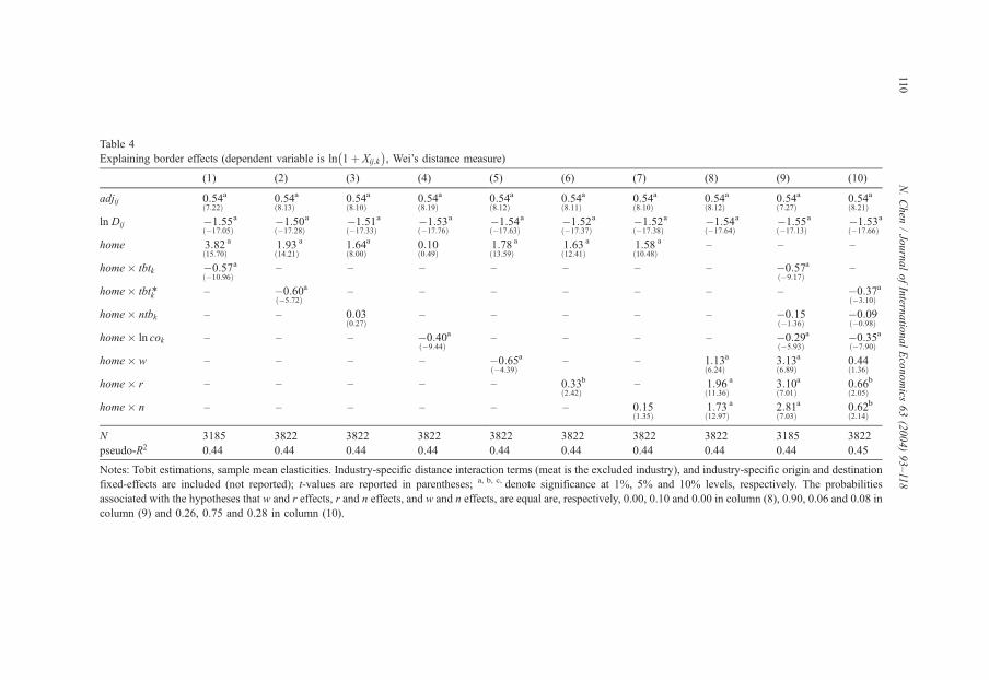
Table 4

Explaining border effects (dependent variable is ln 1þ Xij;k

� �, Wei’s distance measure)

(1) (2) (3) (4) (5) (6) (7) (8) (9) (10)

adjij 0:54ð7:22Þ

a 0:54ð8:13Þ

a 0:54ð8:10Þ

a 0:54ð8:19Þ

a 0:54ð8:12Þ

a 0:54ð8:11Þ

a 0:54ð8:10Þ

a 0:54ð8:12Þ

a 0:54ð7:27Þ

a 0:54ð8:21Þ

a

ln Dij �1:55ð�17:05Þ

a �1:50ð�17:28Þ

a �1:51ð�17:33Þ

a �1:53ð�17:76Þ

a �1:54ð�17:63Þ

a �1:52ð�17:37Þ

a �1:52ð�17:38Þ

a �1:54ð�17:64Þ

a �1:55ð�17:13Þ

a �1:53ð�17:66Þ

a

home 3:82ð15:70Þ

a 1:93ð14:21Þ

a 1:64ð8:00Þ

a 0:10ð0:49Þ

1:78ð13:59Þ

a 1:63ð12:41Þ

a 1:58ð10:48Þ

a – – –


a – – – – – – – �0:57ð�9:17Þ

a –

home� tbtk* – �0:60ð�5:72Þ

a – – – – – – – �0:37ð�3:10Þ

a


– – – – – �0:15ð�1:36Þ

�0:09ð�0:98Þ

home� ln cok – – – �0:40ð�9:44Þ

a – – – – �0:29ð�5:93Þ

a �0:35ð�7:90Þ

a

home� w – – – – �0:65ð�4:39Þ

a – – 1:13ð6:24Þ

a 3:13ð6:89Þ

a 0:44ð1:36Þ

home� r – – – – – 0:33ð2:42Þ

b – 1:96ð11:36Þ

a 3:10ð7:01Þ

a 0:66ð2:05Þ

b

home� n – – – – – – 0:15ð1:35Þ

1:73ð12:97Þ

a 2:81ð7:03Þ

a 0:62ð2:14Þ

b

N 3185 3822 3822 3822 3822 3822 3822 3822 3185 3822

pseudo-R2 0.44 0.44 0.44 0.44 0.44 0.44 0.44 0.44 0.44 0.45





N.Chen

/JournalofIntern

atio

nalEconomics

63(2004)93–118

110

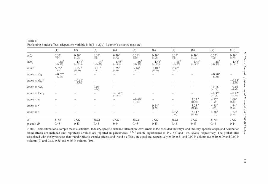
Table 5

Explaining border effects (dependent variable is lnð1þ Xij;kÞ, Leamer’s distance measure)

(1) (2) (3) (4) (5) (6) (7) (8) (9) (10)

adjij 0:57ð7:67Þ

a 0:59ð8:67Þ

a 0:59ð8:63Þ

a 0:59ð8:76Þ

a 0:59ð8:65Þ

a 0:59ð8:63Þ

a 0:59ð8:63Þ

a 0:59ð8:65Þ

a 0:57ð7:76Þ

a 0:59ð8:77Þ

a

lnDij �1:48ð�16:17Þ

a �1:44ð�16:23Þ

a �1:44ð�16:22Þ

a �1:45ð�16:59Þ

a �1:46ð�16:37Þ

a �1:44ð�16:23Þ

a �1:45ð�16:25Þ

a �1:46ð�16:37Þ

a �1:48ð�16:30Þ

a �1:45ð�16:57Þ

a

home 5:55ð25:54Þ

a 3:29ð33:53Þ

a 3:01ð16:52Þ

a 1:25ð6:65Þ

a 3:14ð34:27Þ

a 3:01ð32:66Þ

a 2:92ð24:77Þ

a – – –


a – – – – – – – �0:70ð�11:31Þ

a –

home� tbtk* – �0:60ð�5:76Þ

a – – – – – – – �0:35ð�2:97Þ

a


– – – – – �0:16ð�1:50Þ

�0:10ð�1:05Þ

home� lncok – – – �0:45ð�10:83Þ

a – – – – �0:35ð�7:29Þ

a �0:42ð�9:51Þ

a

home� w – – – – �0:60ð�4:11Þ

a – – 2:53ð16:36Þ

a 4:97ð11:39Þ

a 1:60ð5:26Þ

a

home� r – – – – – 0:24ð1:75Þ

c – 3:25ð22:40Þ

a 4:65ð10:93Þ

a 1:64ð5:36Þ

a

home� n – – – – – – 0:19ð1:68Þ

c 3:11ð32:57Þ

a 4:38ð11:52Þ

a 1:72ð6:37Þ

a

N 3185 3822 3822 3822 3822 3822 3822 3822 3185 3822

pseudo-R2 0.43 0.43 0.43 0.44 0.43 0.43 0.43 0.43 0.44 0.44





N.Chen

/JournalofIntern

atio

nalEconomics

63(2004)93–118

111


where b1;k are the 78 industry-specific home coefficients obtained from the industry-

specific gravity equations reported in Table 2, X denotes the set of explanatory variables, ais a vector of parameters to be estimated and gk is an error term. In Eq. (4), the dependent

variable consists of estimated coefficients with different significance levels, introducing

heteroskedasticity. To control for this, we apply weighted-least-squares where the weights

are given by the inverse of the standard errors of the home coefficients (Head and Mayer,

2000).

The results are reported in Table 6. They are very similar to our previous findings:

industries where TBTs were removed or do not exist (columns (1) and (2)) display smaller

border effects; non-tariff barriers are not significant (column (3)); the spatial agglomer-

ation of firms is associated with larger border effects (column (4)); in column (5), where

the constant term is replaced by three dummies specific to Rauch’s (1999) industry types,

the coefficients on r -type and n -type industries are not significantly different but are

significantly larger than the one for w -type industries, providing some evidence that

product-specific information costs matter.

When all factors are taken together in a single regression (with the tbtk variable), it can

be seen, from column (6), that the significance and signs of the coefficients are generally

preserved (the sample is restricted to those industries affected by TBTs, i.e. N ¼ 65). Note

that the coefficient on tbtk* is insignificant (column (7)).

We also regress the industry-specific home coefficients, obtained with Wei and Leamer

distances, on the various variables. Given that the ranking of home coefficients across

industries was not much affected by the use of different distance measures, we expect

similar conclusions to hold. The results are reported in Tables 7 and 8. The economic

interpretation of the estimated coefficients is indeed similar to that in Table 6, but with a

few exceptions. In Table 8 (Leamer distances), the coefficient on tbtk*, in column (2), is not

significantly different from zero. In column (6), the coefficients on the three categories of

goods distinguished on the basis of information costs are not statistically different from

one another. Finally, in column (7), non-tariff barriers become significant (at the 10%

level) but display a negative coefficient, so that industries affected by NTBs display

smaller border effects. This is however contrary to what could be expected a priori, so we

remain skeptical about this result.

Finally, one might be concerned about the degree to which ready-mix concrete is

driving the results. Recall that the home coefficient for ready-mix concrete, whatever the

distance measure used, is nearly four times that of the next largest industry, and so is a

clear outlier. As a final form of sensitivity analysis, all regressions were therefore re-

estimated when excluding ready-mix concrete from the sample, but the results generally

remain similar to those reported here. Those robustness checks are not reported in order to

save space (but are available from the author upon request).

Our empirical results, which tend to be robust to the use of alternative measures of

distances, to two different econometric approaches and to the exclusion of ready-mix

concrete, provide some support for the role of trade costs in explaining border effects.

Technical barriers to trade, together with product-specific information costs, matter in

explaining border effects across industries, a result which the previous literature has

failed to find. It can thus be argued that deeper market integration, through the removal

of trade barriers and of TBTs in particular, should allow to decrease border effects.

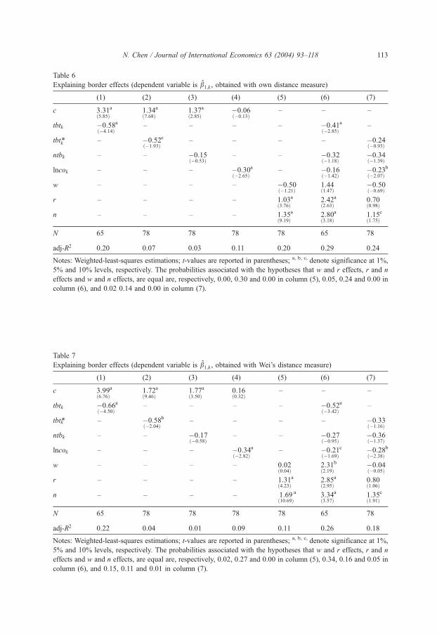
Table 6

Explaining border effects (dependent variable is b1;k , obtained with own distance measure)

(1) (2) (3) (4) (5) (6) (7)

c 3:31ð5:85Þ

a 1:34ð7:68Þ

a 1:37ð2:85Þ

a �0:06ð�0:13Þ

– – –

tbtk �0:58ð�4:14Þ

a – – – – �0:41ð�2:85Þ

a –

tbtk* – �0:52ð�1:93Þ

c – – – – �0:24ð�0:93Þ

ntbk – – �0:15ð�0:53Þ

– – �0:32ð�1:18Þ

�0:34ð�1:39Þ

lncok – – – �0:30ð�2:65Þ

a – �0:16ð�1:42Þ

�0:23ð�2:07Þ

b

w – – – – �0:50ð�1:21Þ

1:44ð1:47Þ

�0:50ð�0:69Þ

r – – – – 1:03ð3:76Þ

a 2:42ð2:63Þ

a 0:70ð0:98Þ

n – – – – 1:35ð9:19Þ

a 2:80ð3:18Þ

a 1:15ð1:75Þ

c

N 65 78 78 78 78 65 78

adj-R2 0.20 0.07 0.03 0.11 0.20 0.29 0.24

Notes: Weighted-least-squares estimations; t-values are reported in parentheses; a, b, c, denote significance at 1%,

5% and 10% levels, respectively. The probabilities associated with the hypotheses that w and r effects, r and n

effects and w and n effects, are equal are, respectively, 0.00, 0.30 and 0.00 in column (5), 0.05, 0.24 and 0.00 in

column (6), and 0.02 0.14 and 0.00 in column (7).

Table 7

Explaining border effects (dependent variable is b1;k , obtained with Wei’s distance measure)

(1) (2) (3) (4) (5) (6) (7)

c 3:99ð6:76Þ

a 1:72ð9:46Þ

a 1:77ð3:50Þ

a 0:16ð0:32Þ

– – –

tbtk �0:66ð�4:50Þ

a – – – – �0:52ð�3:42Þ

a –

tbtk* – �0:58ð�2:04Þ

b – – – – �0:33ð�1:16Þ

ntbk – – �0:17ð�0:58Þ

– – �0:27ð�0:95Þ

�0:36ð�1:37Þ

lncok – – – �0:34ð�2:82Þ

a – �0:21ð�1:69Þ

c �0:28ð�2:38Þ

b

w – – – – 0:02ð0:04Þ

2:31ð2:19Þ

b �0:04ð�0:05Þ

r – – – – 1:31ð4:23Þ

a 2:85ð2:95Þ

a 0:80ð1:06Þ

n – – – – 1:69ð10:69Þ

a 3:34ð3:57Þ

a 1:35ð1:91Þ

c

N 65 78 78 78 78 65 78

adj-R2 0.22 0.04 0.01 0.09 0.11 0.26 0.18




column (6), and 0.15, 0.11 and 0.01 in column (7).


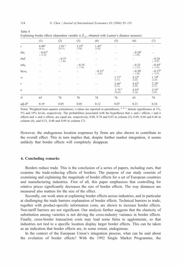
Table 8

Explaining border effects (dependent variable is b1;k , obtained with Leamer’s distance measure)

(1) (2) (3) (4) (5) (6) (7)

c 4:98ð9:51Þ

a 2:81ð16:71Þ

a 3:25ð7:06Þ

a 1:42ð3:26Þ

a – – –

tbtk �0:61ð�4:76Þ

a – – – – �0:54ð�3:99Þ

a –

tbtk* – �0:37ð�1:44Þ

– – – – �0:24ð�0:93Þ

ntbk – – �0:35ð�1:36Þ

– – �0:32ð�1:25Þ

�0:45ð�1:78Þ

c

lncok – – – �0:31ð�2:95Þ

a – �0:20ð�1:86Þ

c �0:27ð�2:51Þ

b

w – – – – 1:71ð3:71Þ

a 4:22ð4:43Þ

a 1:74ð2:29Þ

b

r – – – – 2:66ð9:13Þ

a 4:42ð5:02Þ

a 2:29ð3:17Þ

a

n – – – – 2:75ð18:65Þ

a 4:55ð5:38Þ

a 2:55ð3:82Þ

a

N 65 78 78 78 78 65 78

adj-R2 0.19 0.05 0.05 0.12 0.07 0.21 0.16




column (6), and 0.31, 0.40 and 0.09 in column (7).


However, the endogenous location responses by firms are also shown to contribute to

the overall effect. This in turn implies that, despite further market integration, it seems

unlikely that border effects will completely disappear.

6. Concluding remarks

Borders reduce trade. This is the conclusion of a series of papers, including ours, that

examine the trade-reducing effects of borders. The purpose of our study consists of

examining and explaining the magnitude of border effects for a set of European countries

and manufacturing industries. First of all, this paper emphasizes that controlling for

relative prices significantly decreases the size of border effects. The way distances are

measured also matters for the size of the effect.

Secondly, our work aims at explaining border effects across industries, and in particular

at challenging the trade barriers explanation of border effects. Technical barriers to trade,

together with product-specific information costs, are shown to increase border effects.

Non-tariff barriers are not significant. Our analysis further suggests that the elasticity of

substitution among varieties is not driving the cross-industry variance in border effects.

Finally, cross-border transaction costs may lead some firms to agglomerate, so that

industries not tied to a specific location display larger border effects. This can be taken

as an indication that border effects are, to some extent, endogenous.

In the context of the European Union’s integration process, what can be said about

the evolution of border effects? With the 1992 Single Market Programme, the


abolition of border controls on intra-EU trade, as well as the harmonization or mutual

recognition of standards and other regulations, were intended to increase intra-EU

competition and hence intra-EU trade. Accordingly, and as suggested by our results

relating to TBTs, further market integration should reduce, to a certain extent, the

magnitude of border effects. Monetary Union should also stimulate intra-EU trade and

reduce border effects by increasing transparency between markets. Border effects can

therefore be expected to decrease in the future, but given that they also reflect the

optimal location choices of producers, it seems unlikely that they will fully disappear.

Acknowledgements

This paper is based on Chapter 2 of my Ph.D. dissertation at the Universite Libre de

Bruxelles and is a revised version of CEPR Discussion Paper 3407. I especially wish to

thank Andre Sapir, my thesis supervisor, for his very precious help and advice. I am

grateful to Micael Castanheira, Christophe Croux, Victor Ginsburgh, Philippe Weil, Oved

Yosha and seminar participants at ULB, the CEPR European Research Workshop in

International Trade (ERWIT) and the Leverhulme Centre for Research on Globalisation

and Economic Policy at Nottingham University. I would also like to thank the Editor,

James Harrigan, and two anonymous referees for extremely helpful comments and

suggestions. Financial support from the research network on ‘The Analysis of

International Capital Markets: Understanding Europe’s Role in the Global Economy’,

funded by the European Commission under the Research Training Network Programme

(Contract No. HPRN-CT-1999-00067), is gratefully acknowledged.

Appendix A. The measurement of intra-national and international distances

First, in order to distinguish the regions of a country in terms of economic activity, the

share sm of each region m19 in the country’s GDP is calculated for 1996,

sm ¼ GDPm

GDP

� �

International distances

Using the latitudes and longitudes of the main city in each region, all bilateral distances

between the cities of both countries are calculated by the ‘great circle distance’ formula

which is based on the assumption that the earth is a true sphere (Fitzpatrick and Modlin,

1986). All distances are then each weighted by the GDP share of both regions in the total,

giving more weight to regions with the strongest economic activity (and which should be

more involved in trade).

19 The data are provided at the NUTS-2 level which is the Eurostat nomenclature of statistical territorial

units, subdividing the 15 EU countries into 206 NUTS-2 regions.

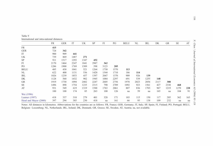
Table 9

International and intra-national distances

FR GER IT UK SP FI PO BELU NL IRL DK GR SE AT

FR 415

GER 724 342

IT 900 909 441

UK 739 869 1487 271

SP 911 1517 1293 1347 452

FI 2170 1464 2247 1841 2987 362

PO 1286 1900 1769 1509 598 3123 205

BELU 485 430 1041 521 1264 1730 1570 113

NL 622 400 1131 536 1420 1544 1710 186 114

IRL 1026 1239 1853 457 1397 2047 1370 909 926 139

DK 1128 560 1432 902 1945 1084 2297 691 539 1255 148

GR 1919 1730 1094 2482 2247 2605 2756 1978 2023 2856 2117 308

SE 1496 890 1754 1235 2315 790 2709 1092 923 1561 427 2330 468

AT 931 549 619 1319 1588 1763 2061 807 836 1703 967 1219 1270 228

Wei (1996)

100 100 174 85 263 100 126 na 59 na 165 na 104 91

Leamer (1997) 418 337 310 279 401 328 171 103 115 150 117 205 362 163

Head and Mayer (2000) 397 294 385 230 418 na 161 66 95 138 109 232 na na

Notes: All distances in kilometres. Abbreviations for the countries are as follows: FR, France; GER, Germany; IT, Italy; SP, Spain; FI, Finland; PO, Portugal; BELU,

Belgium–Luxemburg; NL, Netherlands; IRL, Ireland; DK, Denmark; GR, Greece; SE, Sweden; AT, Austria; na, not available.

N.Chen

/JournalofIntern

atio

nalEconomics

63(2004)93–118

116

Domestic distances

In each country, distances between the main city of each region are first obtained by

applying the ‘great circle distance’ formula (as in the case of international distances). For

each country, intra-national distances are then given by the average of these distances

between the regions of the country, each weighted by the GDP share of both regions in the

total, so that the role of the most economically relevant regions in a country is again

emphasized.

Note that this method permits the calculation of both intra- and international distances

using the same methodology. This is quite similar to Head and Mayer (2000) except that

they use the share of two-digit industry level employment for origin weights and GDP for

destination weights.

Table 9 reports, for each EU member state, our international and intra-national distances

(kms) as well as the internal distances computed by the methods of Wei (1996), Leamer

(1997) and Head and Mayer (2000). One can first note that Wei’s (1996) domestic

distances are, in all cases, much smaller than those obtained by Leamer (1997), Head and

Mayer (2000) and by us. Our results are similar to those of Leamer (1997), but our intra

distance is larger in the case of Italy, perhaps reflecting the particular length of that

country. Further, note that our intra-national distances are larger than those of Head and

Mayer (2000), but this observation also holds for our international distances. However, the

estimation of border effects depends first of all on the relative magnitudes of external and

internal distances. Hence, it is very important to obtain measures of internal distances that

preserve the true ratio between intra- and international distances. So despite our larger

magnitudes for both intra- and international distances, the correlation between our

distances (both inter and intra) with those of Head and Mayer (2000) is equal to 0.985.


References

Anderson, J.E., van Wincoop, E., 2001. Gravity with gravitas: a solution to the border puzzle. National Bureau of

Economic Research Working Paper 8079.

Boisso, D., Ferrantino, M., 1997. Economic distance, cultural distance, and openness in international trade:

empirical puzzles. Journal of Economic Integration 12 (4), 456–484.

Cyrus, T.L., 2000. Why do national borders matter? Industry-level evidence. Dalhousie University, mimeo.

Eichengreen, B., Irwin, D.A., 1993. Trade blocs, currency blocs and the disintegration of world trade in the

1930s. Centre for Economic Policy Research Discussion Paper 837.

Eichengreen, B., Irwin, D.A., 1998. The role of history in bilateral trade flows. In: Frankel, J.A. (Ed.), The

Regionalization of the World Economy. The University of Chicago Press, pp. 33–57.

Ellison, G., Glaeser, E.L., 1994. Geographic concentration in US manufacturing industries: a dartboard approach.

National Bureau of Economic Research Working Paper 4840.

Ellison, G., Glaeser, E.L., 1997. Geographic concentration in US manufacturing industries: a dartboard approach.

Journal of Political Economy 105 (5), 889–927.

European Commission, 1997. Trade Creation and Trade Diversion. The Single Market Review, Subseries IV:

Impact on Trade and Investment 3.

European Commission, 1998. Technical Barriers to Trade. The Single Market Review, Subseries III: Dismantling

of Barriers 1.

Evans, C.L., 1999. The economic significance of national border effects. Federal Reserve Bank of New York,

mimeo.


Evans, C.L., 2001. Border effects and the availability of domestic products abroad. Federal Reserve Bank of New

York, mimeo.

Fitzpatrick, G.L., Modlin, M.J., 1986. Direct-Line Distances, International Edition The Scarecrow Press, Inc,

Metuchen, NJ and London.

Grossman, G.M., 1998. Comment on Deardorff, A.V., Determinants of bilateral trade: does gravity work in a

neoclassical world? In: Frankel, J.A. (Ed.), The Regionalization of the World Economy. The University of

Chicago Press, pp. 29–31.

Hazledine, T., 2000. How much do national borders matter? Helliwell, J.F.’s book review. The Canadian Journal

of Economics 33 (1), 288–292.

Head, K., Mayer, T., 2000. Non-Europe: the magnitude and causes of market fragmentation in the EU. Welt-

wirtschaftliches Archiv 136 (2), 285–314.

Head, K., Mayer, T., 2001. Illusory border effects: distance mismeasurement inflates estimates of home bias in

trade. University of British Columbia, mimeo.

Helliwell, J.F., 1995. Do national borders matter for Quebec’s trade? National Bureau of Economic Research

Working Paper 5215.

Helliwell, J.F., 1997. National borders, trade and migration. National Bureau of Economic Research Working

Paper 6027.

Helliwell, J.F., 1998. How Much Do National Borders Matter? The Brookings Institution, Washington D.C.

Helliwell, J.F., 2000. Measuring the width of national borders. University of British Columbia, mimeo.

Helliwell, J.F., Verdier, G., 2000. Comparing interprovincial and intraprovincial trade densities. University of

British Columbia, mimeo.

Hillberry, R., 1999. Explaining the ‘border effect’: what can we learn from disaggregated commodity flow data?

Indiana University Graduate Student Economics Working Paper Series 9802. Indiana University.

Hillberry, R., 2001. Aggregation bias, compositional change, and the border effect. US International Trade

Commission, mimeo.

Hillberry, R., Hummels, D., 2000. Explaining home bias in consumption: production location, commodity

composition and magnification. Purdue University, mimeo.

Hillberry, R., Hummels, D., 2002. Intra-national home bias: some explanations. National Bureau of Economic

Research Working Paper 9022.

Hummels, D., 1999a. Toward a geography of trade costs. Purdue University, mimeo.

Hummels, D., 1999b. Transportation costs and international integration in recent history. Purdue University,

mimeo.

Leamer, E.E., 1997. Access to western markets, and eastern effort levels. In: Zecchini, S. (Ed.), Lessons from the

Economic Transition: Central and Eastern Europe in the 1990s. Kluwer Academic Publishers, pp. 503–526.

McCallum, J., 1995. National borders matter: Canada–US regional trade patterns. American Economic Review

85 (3), 615–623.

McDonald, J.F., Moffitt, R.A., 1980. The uses of tobit analysis. Review of Economics and Statistics 62 (2),

318–321.

Nitsch, V., 2000a. National borders and international trade: evidence from the European Union. Canadian Journal

of Economics 33 (4), 1091–1105.

Nitsch, V., 2000b. It’s not right but it’s okay: on the measurement of intra- and international trade distances.

Humboldt University Berlin, mimeo.

Rauch, J.E., 1999. Networks versus markets in international trade. Journal of International Economics 48 (1),

7–35.

Rose, A.K., van Wincoop, E., 2001. National money as a barrier to international trade: the real case for currency

union. American Economic Review 91 (2), 386–390.

Wei, S.-J., 1996. Intra-national versus international trade: how stubborn are nations in global integration?

National Bureau of Economic Research Working Paper 5531.

Wolf, H.C., 1997. Patterns of intra- and inter-state trade. National Bureau of Economic Research Working Paper

5939.

Wolf, H.C., 2000a. Intranational home bias in trade. Review of Economics and Statistics 82 (4), 555–563.

Wolf, H.C., 2000b. (Why) Do borders matter for trade? In: Hess, G.D., van WINCOOP, E. (Eds.), Intra-

national Macroeconomics. Cambridge University Press, pp. 112–128.

intra-national versus international trade in the european union: why do national borders matter?

Documents