intraday patterns in the cross-sectional of stock returns

African Journal of Business Management Vol. 5(27), pp. 11116-11130, 9 November, 2011 Available online at http://www.academicjournals.org/AJBM DOI: 10.5897/AJBM11.1177 ISSN 1993-8233 ©2011 Academic Journals

Full Length Research Paper

Intraday patterns in the cross-sectional of stock returns: Dow Jones Industrial Average (DJIA) and

National Association of Securities Dealers Automated Quotations (NASDAQ) high frequency indexes

Hai-Chin Yu1, Chia-Yi Wu2 and Der-Tzon Hsieh*

1Department of International Business, Chung-Yuan University, Chungli, Taiwan.

2Institute of Economics, Academia Sinica, Taipei, Taiwan.

3Department of Economics, National Taiwan University, Taipei, 100, Taiwan.

Accepted 27 July, 2011

This paper examines the behavior of intra-day periodicity by dividing the trading day into 39 and 10 min trading intervals for both the Dow Jones and NASDAQ markets. Using a high frequency data of 10 min stock index over the period of August 1, 1997 to June 19, 2007, which included 2,485 trading days with 96,915 intraday observations, we found that the current return today has a positive and explanatory impact on the return at the same time tomorrow. Results of this study are in line with the reports by Heston et al. (2010) who use diversified individual common stocks rather than stock indexes, implying the negative autocorrelation induced by bid-ask bounce and lack of resiliency in both DJIA and NASDAQ markets as well. Although, there is a significant positive relation between a stock’s return over an interval and its subsequent returns at daily frequencies, this effect is found significant for only one day for DJIA, whereas up to around five trading days for NASDAQ. No significant size effect differences were found between both market traders and neither was intraday patterns changed after the event of 911 shocks. Key words: Microstructure, trading strategies, institutional investors, intraday behavior.

INTRODUCTION The modern electronic trading and monitoring systems have increasingly influenced the investors’ behaviors in stock markets. Market participants are now better equipped to monitor price movements within a day. These developments make the transmission of information more efficient among both institutional and individual investors, and in turn foster the trading activity in a higher frequency. These more frequent trading behaviors make intraday patterns significantly different than they were before when trading orders were placed via brokers or phones. Over the past few decades, several studies have documented the phenomenon of seasonal effects, that is,

*Corresponding author E-mail: [email protected]. Tel: 886223974382. Abbreviations: EST, Eastern time zone; DJIA, Dow Jones Industrial Average; NYSE, New York Stock Exchange.

the weekend effect or January effect (for example, Cross, 1973; French, 1980; Gibbons and Hess, 1981; Lakonishok and Levi, 1982; Harris, 1986). However, if investors have manipulated their trading strategy on the basis of these informed rules, how can these arbitrage opportunities and seasonal effects still appear? We postulate that systematic trading from huge institutional fund flows may lead to predictable patterns in trading volume and price among diversified stocks. Finally, these behaviors may make the stock index a meaningful indicator that deserves to be used to further explore the cross-sectional patterns among different periods in each day. Heston et al. (2010) find evidence of periodicity in the cross-section of stock returns, implying that these patterns are not fully anticipated by all of the investors and that some unsystematic noises still exist that merit closer attention. In a modern financial system, the rapid development of information technology has enabled in-vestors to trade more efficiently and to save more costs

via electronic trading systems (Marcel and Phelps, 1994). These shorter trading intervals may contain a lot more micro information regarding regular trading behaviors than would be possible with daily or monthly returns.

Furthermore, the trading algorithms may also affect intraday return patterns. For example, large financial institutions might be buying the same set of stocks at the same time of the day during each trading day because they are following an indexing strategy program or a quantitative investment strategy, which causes these institutions to trade similar securities in the same direction (Heston et al., 2010). They conclude that a statistically significant positive relationship exists between an individual stock return over an interval and its subsequent returns at daily frequencies (that is, lags of 13, 26 and 39 ... periods) for up to forty days. Although, evidence shown that intraday patterns appear in the cross-sectional of diversified common stocks, however, there is a lack of studies that examine the whole stock index return at a specified interval and its following returns at the same interval the next day and on subsequent days. Our paper fills this gap and provides an overall conclusion based on the notation of the market portfolio index instead of some selective and individual stocks. We doubt, if it is a fact that these trading systems or trading algorithms have changed investors’ trading behaviors and influenced intraday effects over time. Then, if the trading time effect based on shorter intervals has been increasing, the trading pattern based on longer intervals of the weekend or January effect has been diminishing? Owing to institutional investors accounting for over 70% of trading volume in the United State securities markets, using the stock index should be a more representative measure for the market as a whole than some individual stocks. The extant literature finds substantial evidence that flows of funds to certain types of institutional investors exhibit autocorrelation (Del Guercio and Tkac, 2002; Frazzini and Lamont, 2008; Lou, 2008; Blackburn et al., 2007). Campbell et al. (2009) suggest that institutional investors prefer to buy or sell the same stocks on successive days, implying that institutional trading is highly persistent.

This persistent behavior causes the intraday returns to be affected by the previous days or to be similar to the previous days. For an experienced manager, it would be natural and expedient to execute these orders at speci-fied times of the day to leave the remaining time available for other research and risk management activities. By doing so, the patterns of trading behavior across different times may be different, and the patterns at closing to near-closing interval, or opening to after-opening may vary. Our paper contributes to the current literature in several crucial ways. By dividing the trading day into 39 ten

minute trading intervals from 96,915 intraday observations of DJIA (Dow Jones Industrial Average 30) and NASDAQ (NASDAQ 100) indexes, some interesting evidence is obtained. First, we employ DJIA and NASDAQ composite indices to analyze our empirical results. In general, people

Yu et al. 11117 people are of the opinion that it is easier for small-scale stocks to give rise to intraday effects than large-scale stocks. However, have large-scale stocks fully hedged this effect? In our study, the DJIA represents the most well-established and financially-sound large-scale companies in the US market, while the NASDAQ consists of highly volatile and high-tech small-scale companies. Using both of them in our study can provide a clear view of United State stock markets.

It can also prove whether the size effect affects the intraday effect. In our study, we find that either the DJIA or NASDAQ exhibits a pattern resembling an intraday pattern, implying that investors’ trading behaviors are not affected by the change in the scale of companies. Second, in contrast to Heston et al. (2010) focus on New York Stock Exchange (NYSE) stocks for 2001 to 2005, we look at both DJIA and NASDAQ stocks over a longer period from August 1, 1997 to June 19, 2007 spanning several events that allow us to examine extra dimension with event of shocks regarding securities markets. We therefore perform a robustness test based on sub-period analysis both pre-911 and post-911. Our evidence shows that the 911 event does not significantly affect the intra-day effect, implying that, in general, trading behaviors are not altered by financial shock events. Third, compared with Heston et al. (2010), our analysis employs a weighted average index instead of diversified common stocks to verify the intraday effects. While individual stocks are employed, researchers must first filter out highly active stocks from those individual stocks. In so doing, some difficulties may be encountered in choosing appropriate samples. Nevertheless, index stocks have weighted all of the individual stocks, and so we can avoid the biases of sampling. Finally, in contrast to the previous literature using time series models Andersen et al. (2000), in which Andersen et al. (1997) investigate intraday effects, we follow the cross-sectional regression methodology of Jegadeesh (1990). Based on this cross-section regression model, we can not only consider the information of time series but also the information of cross-sectional data across different trading intervals during a day. In our study, the estimates of lag 39 (the daily interval) reveal a significantly positive value in either the DJIA or NASDAQ stock markets. It means that the current return today has a positive and explanatory effect on the return at the same time tomorrow. The remaining part of this paper are organized as follows. the methodology employed, discusses the empirical results, and presents the conclusions.

DATA DESCRIPTION AND METHODOLOGY

Our data are composed of the DJIA and the NASDAQ indexes 10-minute intraday returns provided by the Bloomberg real-time data

service. The 10-minute returns for both the DJIA and the NASDAQ stocks extend from August 1, 1997 to June 19, 2007, including 2,485 trading days with 96,915 intraday observations from 9:30 to

11118 Afr. J. Bus. Manage. 15:50 EST (Eastern Time Zone). The DJIA represents the largest, most well-established and financially sound companies, whereas the NASDAQ consists of smaller, higher growth technology companies. These two indexes represent not only the core of the United State economy but also allow us to verify whether there are size-related differences in any observed intraday effects. Our study seeks to examine the intraday patterns which include the time series effects and different trading time effects at the same time. Jegadeesh (1990) provides a suitable model for our study. As a result, we analyze intraday effects by extending Jegadeesh’s cross-sectional regression model. The multivariate cross-sectional regression is specified as follows:

1 , 1 2 , 2 39 , 39it t t i t t i t t i t itr r r r e (1)

where itr is the return at the ith trading time on the tth trading day

(i=1, 2, …,39 while t=1,2,…,2485). The cross-sectional regressions are calculated from August 1

st, 1997 through June 19

th, 2007

covering 2,485 trading days. The slope coefficients

1 2 39, ,...,t t t represent the response of returns at 10 min

intervals to returns over a previous interval. Therefore, we call these slope coefficients “return responses”. In addition to the multivariate regressions of Equation (1), we also run simple regressions of 10 min stock returns on returns lagged by daily frequencies (lag 39, 78, 117, 156, 195,…,780).

,it tk i t k itr r e (2)

Where the slope coefficients tk represent the response of returns

at itr to returns over a previous interval lagged by k 10 min

intervals. In this study, we seek to investigate the interday effect, and so the k are specified as daily frequencies, that is, k = 39, 78, 117… 780.

EMPIRICAL RESULTS AND ANALYSES Cross-section intraday statistics summaries In order to investigate the intraday pattern, we reshape the entire 10 min returns into a panel format containing 39 cross-sections that depend on different trading times (9:30, 9:40, …, 15:50). Figure 1 displays the corresponding means and volatilities (standard devi-ations) across 39 trading intervals in each day. In Figure 1, the opening time at 9:30 contains overnight noise and the information reveals a “high return associated with high risk” phenomenon in either the DJIA (with a mean of 0.0247% and a volatility of 0.5248%) or the NASDAQ (with a mean of 0.0821% and a volatility of 1.1338%). Eventually, the closing time of 15:30 also reveals a remarkable, positive return (with a mean of 0.0038% and a volatility of 0.1486% for the DJIA and a mean of 0.0132% and a volatility of 0.328% for the NASDAQ, respectively). Substantially, a U-shape is found in Figure 1a and b, implying that the intraday pattern may hide some implications of trading behaviors that deserve to be

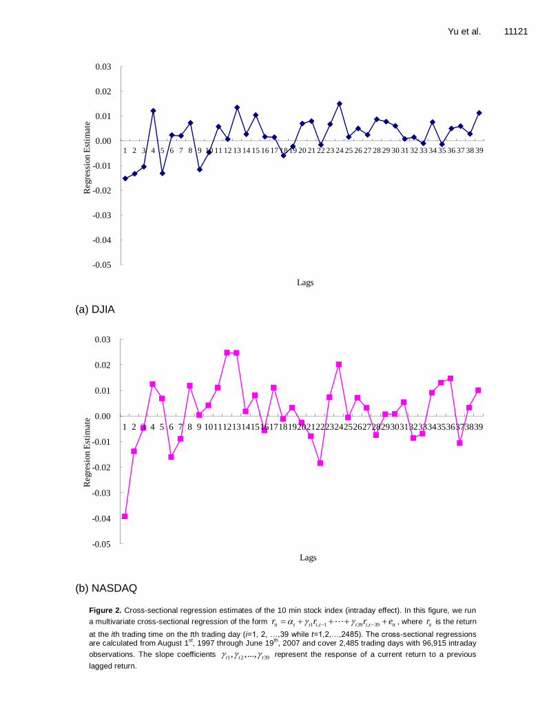
detected. These results are in line with the findings of Wood et al. (1985), Harris (1986), and Jain and Joh (1988) and so on. Return of intraday and interday effects Following the approach of Heston et al. (2010), the “return responses” of the cross-sectional regressions in the DJIA and NASDAQ are presented in Table 1, with the correspondent graphs in Figure 2. In Table 1, the estimates of multivariate regression of Equation (1) in earliest periods are found significantly negative, that is, the regression estimates of the DJIA in lag 1, lag 2 and lag 3 are -0.1512 (t-value=-4.28), -0.0133 (t-value=-3.75), and -0.0104 (t-value=-2.94), respectively; and the regression estimates of the NASDAQ in lag 1 and lag 2 are -0.0392 (t-value=-11.05) and -0.0138 (t-value=-3.88), respectively. These negative results may be related to bid-ask bounce and lack of resilience as suggested by Heston et al. (2010). However, our evidence shows that the estimate of lag 39 is significantly positive, with 0.0114 (t-value=3.24) for the DJIA and 0.0101 (t-value=2.84) for the NASDAQ. This finding means that the current return today has a positive and explanatory impact on the return at the same time tomorrow. Furthermore, results of Table 2 show that the regression estimate of lag 39 in Equation (2) is significantly positive in either the DJIA

( 39 0.0101t , t-value=3.11) or the NASDAQ

( 39 0.0197t , t-value=6.06) market, implying that the

current return today has a positive effect on the return at the same time tomorrow. However, most of the estimates of the DJIA in the following lag periods are not significant, meaning that the weekday effect has been diminishing in the DJIA market. Interestingly, the NASDAQ market exhibits a slightly different result.

In Table 2 and Figure 3, the estimates of lag 39 (Day 1), lag 78 (Day 2), lag 156 (Day 4), and lag 195 (Day 5) are significant, meaning that today’s return in the NASDAQ influences the returns of the following days. However, this effect diminishes gradually after the second week. We interpret the possible reasons are resulting from that DJIA consists of the largest, most well-established and financially sound companies, and the DJIA is more efficient. As a result, the seasonal effect of the DJIA is smaller than that of the NASDAQ. By comparing the response effect of DJIA and NASDAQ, we find that the estimate of the NASDAQ is larger than that of the DJIA, revealing the higher volatility property in the NASDAQ. Besides that, although, the DJIA represents well-established and financially-sound large-scale companies, while the NASDAQ is composed by high-tech small-scale companies, the intraday patterns and return responses between these two markets are similar. Evidence of this finding implies that the size effect does not significantly influence the intraday effect.

Yu et al. 11119

(a) DJIA

(b) NASDAQ

Figure 1. Mean and volatility across different trading times in one day for DJIA and NASDAQ over August 1

st, 1997

to June 19th, 2007.

11120 Afr. J. Bus. Manage.

Table 1. Multivariate regression estimates of cross-sectional regressions of 10 min interval DJIA and NASDAQ returns (August 1

st, 1997 to June 19

th, 2007 covering 2,485 trading days with 96,915

intraday observations).

Variable DJIA NASDAQ

Estimate t-statistic Estimate t-statistic

Lag1 -0.0152 -4.2825***

-0.0392 -11.0534***

Lag2 -0.0133 -3.7467***

-0.0138 -3.8820***

Lag3 -0.0104 -2.9385***

-0.0047 -1.3125

Lag4 0.0122 3.4332***

0.0125 3.5221***

Lag5 -0.0130 -3.6790***

0.0069 1.9475*

Lag6 0.0024 0.6669 -0.0160 -4.4959***

Lag7 0.0021 0.5814 -0.0089 -2.4962**

Lag8 0.0073 2.0704**

0.0118 3.3258***

Lag9 -0.0116 -3.2566***

0.0005 0.1299

Lag10 -0.0046 -1.2891 0.0042 1.1877

Lag11 0.0058 1.6274 0.0111 3.1164***

Lag12 0.0007 0.2055 0.0248 6.9404***

Lag13 0.0135 3.8162***

0.0247 6.9150***

Lag14 0.0027 0.7656 0.0018 0.5105

Lag15 0.0105 2.9598***

0.0081 2.2769**

Lag16 0.0017 0.4857 -0.0056 -1.5718

Lag17 0.0015 0.4251 0.0111 3.1320***

Lag18 -0.0060 -1.6966*

-0.0011 -0.3162

Lag19 -0.0022 -0.6230 0.0033 0.9347

Lag20 0.0071 2.0155**

-0.0025 -0.7073

Lag21 0.0080 2.2904**

-0.0079 -2.2308**

Lag22 -0.0015 -0.4303 -0.0184 -5.1850***

Lag23 0.0067 1.9170*

0.0073 2.0701**

Lag24 0.0150 4.2832***

0.0201 5.6967***

Lag25 0.0016 0.4635 -0.0006 -0.1600

Lag26 0.0050 1.4331 0.0071 2.0104**

Lag27 0.0025 0.7146 0.0032 0.8978

Lag28 0.0088 2.5076**

-0.0074 -2.0962**

Lag29 0.0078 2.2366**

0.0007 0.1988

Lag30 0.0061 1.7430*

0.0008 0.2159

Lag31 0.0008 0.2334 0.0054 1.5361

Lag32 0.0015 0.4262 -0.0086 -2.4313**

Lag33 -0.0010 -0.2732 -0.0069 -1.9328*

Lag34 0.0076 2.1794**

0.0091 2.5735**

Lag35 -0.0013 -0.3822 0.0131 3.6898***

Lag36 0.0051 1.4459 0.0147 4.1413***

Lag37 0.0060 1.7145*

-0.0106 -2.9696***

Lag38 0.0028 0.8051 0.0033 0.9264

Lag39 0.0114 3.2374***

0.0101 2.8420***

Intercept 0.0000 0.7827 0.0000 -0.0214

Observations 96,915 96,915

R2 0.0023 0.0057

Note: This table reports cross-sectional regression results based on Equation (1). *, **, and *** denote significance at the 10, 5, and 1% levels, respectively.

Yu et al. 11121

(a) DJIA

(b) NASDAQ

-0.05

-0.04

-0.03

-0.02

-0.01

0.00

0.01

0.02

0.03

1 2 3 4 5 6 7 8 9 10 11 12 13 14 15 16 17 18 19 20 21 22 23 24 25 26 27 28 29 30 31 32 33 34 35 36 37 38 39

Reg

ress

ion

Est

imat

e

Lags

-0.05

-0.04

-0.03

-0.02

-0.01

0.00

0.01

0.02

0.03

1 2 3 4 5 6 7 8 9 101112131415161718192021222324252627282930313233343536373839

Reg

resi

on

Est

imat

e

Lags

Figure 2. Cross-sectional regression estimates of the 10 min stock index (intraday effect). In this figure, we run

a multivariate cross-sectional regression of the form 1 , 1 39 , 39it t t i t t i t itr r r e , where itr is the return

at the ith trading time on the tth trading day (i=1, 2, …,39 while t=1,2,…,2485). The cross-sectional regressions are calculated from August 1


th, 2007 and cover 2,485 trading days with 96,915 intraday

observations. The slope coefficients 1 2 39, ,...,t t t represent the response of a current return to a previous

lagged return.


Table 2. Univariate estimates of cross-sectional regressions of 10 min interval DJIA and NASDAQ returns for interday effects (August 1

st, 1997 to June 19

th, 2007 covering 2,485 trading days with

96,915 intraday observations).

DJIA NASDAQ

Variable Estimate t-statistic Estimate t-statistic

Lag39 (Day 1 of 1stweek) 0.0101 3.1113

** 0.0197 6.0568

***

Lag78 (Day 2 of 1stweek) 0.0007 0.2216 -0.0082 -2.5322

**

Lag117 (Day 3 of 1stweek) -0.0003 -0.1070 -0.0051 -1.5508

Lag156 (Day 4 of 1stweek) 0.0082 0.0120 0.0154 4.6839

***

Lag195 (Day 5 of 1stweek) 0.0112 0.0006 0.0215 6.5070

***

Lag234 (Day 1 of 2nd

week) 0.0045 1.3651 0.0044 1.3107


week) -0.0027 -0.8419 0.0025 0.7458


week) -0.0006 -0.1764 -0.0031 -0.9153


week) -0.0059 -1.8326 -0.0018 -0.5331


week) -0.0004 -0.1291 -0.0082 -2.4432**

Lag429 (Day 1 of 3rd

week) 0.0027 0.8501 -0.0077 -2.2722**


week) 0.0026 0.8104 0.0070 2.0630**


week) -0.0073 -2.2777**

-0.0028 -0.8393


week) 0.0129 3.9761***

0.0132 3.8806***


week) 0.0040 1.2349 0.0034 0.9857

Lag624 (Day 1 of 4thweek) 0.0003 0.1075 0.0054 1.5685

Lag663 (Day 2 of 4thweek) 0.0022 0.6676 0.0033 0.9823

Lag702 (Day 3 of 4thweek) 0.0056 1.7507 0.0062 1.9061

*

Lag741 (Day 4 of 4thweek) 0.0067 2.0786

** 0.0029 0.8858

Lag780 (Day 5 of 4thweek) -0.0044 -1.3695 0.0079 2.4497

**

This table reports cross-sectional regression results based on Equation (2). *, **, and *** denote significance at the 10, 5, and 1% levels, respectively.

Sub-period analysis and intraday effects: Robustness tests Next, to further explore if intraday patterns are varied with unexpected shocks, we employ a sub-period analysis to examine if the cross-sectional estimates change. To do this, the 911 event was selected to test whether intraday patterns change pre- and post- the event. Both markets reacted strongly to the 911 event in the United States. This event causes the opening of the New York Stock Exchange (NYSE) was delayed, and trading for the day canceled after the second attack of plane crashed. NASDAQ also canceled trading. After halting for four business days and stocks fell sharply in the re-opening days of the stock market, with the DJIA falling 684.81 points to its lowest point (Figure 5). We thus divide the whole sample period into three sub-periods based on this event: 1997/8/1 to 2001/9/20 (pre-event), 2001/9/21 to 2003/6/30 (during-the-event) and 2003/7/1 to 2007/6/19 (post-event). Figure 6 displays the intraday patterns of these sub-periods and it seems that these three periods exhibit the similar patterns. In addition, if the cross-sectional estimate of the lag period is negative, the

second period (during-the-event) has the largest negative value among these three periods. Evidence of this implies that the investors’ trading rules (buy or sell) are not affected by this shocks, the intraday patterns do not change for the unexpected shocks. As for the cross-sectional estimates between pre- and post-911 attack, no significant changes were found for intraday patterns as well.

CONCLUSIONS

This paper compensates for the extant literature, namely, the seasonality field, another dimension of the intraday patterns by using stock indexes that examine the cross-sectional regression estimates rather than by utilizing diversified common stocks. We contribute to the current literature in several important ways. First, the 10 min high frequency data adds another dimension of the speed of information in contrast to the half-hour frequency data of Heston et al. (2010), so that the investors’ belief at the specified time is stronger than those for a specified day, whereas low-frequency data cannot provide enough intraday information. Secondly, large DJIA and small NASDAQ stocks exhibit similar cross-sectional patterns

Yu et al. 11123

(a) Regression estimates

(b) t-value

-0.010

-0.005

0.000

0.005

0.010

0.015

0.020

0.025

39 78 117 156 195 234 273 312 351 390 429 468 507 546 585 624 663 702 741 780

Reg

ress

ion E

stim

ate

Lags

DJIA NASDAQ

-3.0

-2.0

-1.0

0.0

1.0

2.0

3.0

4.0

5.0

6.0

7.0

39 78 117 156 195 234 273 312 351 390 429 468 507 546 585 624 663 702 741 780

t-val

ue

Lags

DJIA NASDAQ

Figure 3. Cross-sectional regressions of 10 min returns (interday effect). In this figure, we run a simple cross-sectional

regression of the form ,it tk i t k itr r e , where the slope coefficients tk represent the response of returns at itr to

returns over a previous interval lagged by k 10 min intervals. Here we seek to investigate the interday effect, and the k are specified as daily frequencies, that is, k =39, 78, 117… 780.


(a) DJIA

(b) NASDAQ

Figure 4. The price movements in the DJIA and NASDAQ markets. The sample period extends from

August 1, 1997 to June 19, 2007 for a total of 2,485 observations. The 911 event in 2001 depressed the US stock market and the index on September 21, 2001 dropped to its lowest point since the 911 event. Thus, we divide the overall sample into three sub-periods: 1997/8/1 to 2001/9/20 (pre-event), 2001/9/21 to 2003/6/30 (during-the-event) and 2003/7/1 to 2007/6/19 (post-event).

as shown in Figures 2(a and b) and 3(a), implying that a size effect does not exist in either the intraday or the interday effect. Thirdly, while the weekend effect has gradually lost much of its momentum and relevance, the

intraday effect and its pattern of cross-sectional estimates seem to contain much more investor behavior information. Our results indicate that almost all of the estimates in the DJIA market are not significant except for

Yu et al. 11125

(a) DJIA

(b) NASDAQ

Figure 5. The return movements of the DJIA and NASDAQ stock indexes (August 1, 1997 to June 19, 2007 for a total

of 2,485 trading days).


(a) DJIA

(b) NASDAQ

-0.05

-0.04

-0.03

-0.02

-0.01

0

0.01

0.02

0.03

0.04

1 3 5 7 9 11 13 15 17 19 21 23 25 27 29 31 33 35 37 39

Reg

ress

ion

Est

imat

e

Lags

1997/8/1~2001/9/21 2001/9/21~2003/6/30 2003/7/1~2007/6/19

-0.05

-0.04

-0.03

-0.02

-0.01

0

0.01

0.02

0.03

0.04

0.05

1 3 5 7 9 11 13 15 17 19 21 23 25 27 29 31 33 35 37 39

Reg

ress

ion E

stim

ate

Lags

1997/8/1~2001/9/20 2001/9/21~2003/6/30 2003/7/1~2007/6/19

Figure 6. Regression estimates of 10-minute stock indexes among three sub-periods: 1997/8/1 to

2001/9/20 (pre-event), 2001/9/21 to 2003/6/30 (during-the-event) and 2003/7/1 to 2007/6/19 (post-event).

lag 39, lag 507, lag 746, and lag 741, revealing that the weekday effect seems to have been diminishing. Fourth, the intraday patterns do not change after the 911 event in our sub-period analysis (Figure 6), meaning that the

cross-sectional measures are quite robust, without being influenced by the unexpected shocks. It also implies that investors’ trading behavior is more tied to a trading time on a certain day, rather than to a specified day during a

week. Fifth, the overall trading behaviors of the DJIA and NASDAQ are quite aligned (complementary) to each other during a day, although they are quite different during a week. REFERENCES

Andersen TG, Bollerslev T (1997). Intraday periodicity and volatility persistence in financial markets. J. Empirical Finance, 4: 115-158.

Andersen TG, Bollerslev T, Cai J (2000). Intraday and interday volatility

in the Japanese stock market. J. Int. Financ. Markets, Inst. Money, 10: 107-130.

Campbell JY, Ramadorai T, Schwartz A (2009). Caught on tape:

Institutional trading, stock returns, and earning announcements. J. Financial Econom., 92: 66-91.

Cross F (1973). The behavior of stock prices on Fridays and Mondays.

Financ. Analysts J., 29(6): 67-69. French KR (1980). Stock returns and the weekend effect. J. Financ.

Econom., 8(1): 55-69.

Yu et al. 11127 Gibbons MR, Hess P (1981). Day of the week effects and asset returns.

J. Bus. 54(4): 579-596. Harris L (1986). A transaction data study of weekly and intradaily

patterns in stock returns. J. Financ. Econom., 16(1): 99-117. Heston SL, Korajczyk RA, Sadka R (2010). Intraday patterns in the

cross-section of stock returns. J. Finance. 65(4): 1369-1407.

Jain PC, Joh GH (1988). The dependence between hourly prices and trading volume. J. Financ. Quant. Anal., 23: 269-283.

Jegradeesh N (1990). Evidence of predictable behavior of security

returns. J. Finance, 45: 991-898. Lakonishok J, Levi M (1982). Weekend effects on stock returns: A note.

J. Finance, 37: 883-889.

Marcel NM, Phelps BD (1994). Electronic trading, market structure and liquidity. Financial Analysts J., pp. 29-50.

Schwartz R, Shapiro J (1992). The challenge of institutionalization for

the equity markets. Recent developments in finance. Anthony Saunders ed. New York University Salomon Center, New York, NY.

Wood RA, Thomas HM, Ord JK (1985). An investigation of transactions

data for NYSE stocks. J. Finance, 40: 723-739.


APPENDIX Table 1a. Preliminary statistics of 10 min intraday returns across cross-sectional trading time

in the DJIA.

Trading time Obs Mean Std dev Skewness Kurtosis

9:30 2485 0.000247 0.005248 -0.028601 4.418365

9:40 2485 -0.000073 0.002234 -1.324743 20.791571

9:50 2485 -0.000031 0.002058 -0.770759 13.602534

10:00 2485 -0.000082 0.002248 0.023509 3.891067

10:10 2485 -0.000045 0.001971 -0.588576 13.946366

10:20 2485 0.000058 0.001680 1.582913 20.509329

10:30 2485 0.000045 0.001682 0.396837 5.266297

10:40 2485 0.000045 0.001551 0.202613 2.749717

10:50 2485 -0.000012 0.001493 0.352048 15.259487

11:00 2485 -0.000006 0.001394 -0.019850 2.534399

11:10 2485 -0.000009 0.001341 0.174827 3.816532

11:20 2485 -0.000025 0.001228 -0.080120 3.236802

11:30 2485 0.000024 0.001256 -0.085681 5.404281

11:40 2485 -0.000015 0.001285 1.082682 20.762991

11:50 2485 -0.000010 0.001269 -1.314515 23.323390

12:00 2485 -0.000039 0.001228 0.334935 7.411716

12:10 2485 -0.000011 0.001133 -0.336241 5.418083

12:20 2485 0.000041 0.001077 -0.323517 9.236881

12:30 2485 0.000014 0.001116 -0.807196 8.331423

12:40 2485 0.000009 0.001102 0.060696 3.856560

12:50 2485 0.000037 0.001128 -0.811379 19.805668

13:00 2485 -0.000023 0.001102 -0.088902 4.430249

13:10 2485 0.000025 0.001305 4.319054 96.408179

13:20 2485 0.000005 0.001228 1.524576 27.765394

13:30 2485 0.000024 0.001212 1.000115 12.197950

13:40 2485 -0.000038 0.001202 0.110516 3.373547

13:50 2485 0.000042 0.001229 0.354604 7.495694

14:00 2485 -0.000067 0.001344 -0.669606 7.231262

14:10 2485 -0.000022 0.001435 0.489851 9.703892

14:20 2485 -0.000018 0.001445 -0.070301 4.923308

14:30 2485 0.000009 0.001483 -0.316569 7.832817

14:40 2485 -0.000015 0.001436 0.221840 4.491354

14:50 2485 0.000001 0.001486 -0.301464 7.044979

15:00 2485 0.000014 0.001634 0.268300 3.590599

15:10 2485 0.000047 0.001568 0.799197 9.577524

15:20 2485 0.000010 0.001658 0.184552 7.935995

15:30 2485 -0.000006 0.001828 -0.594895 7.459044

15:40 2485 0.000018 0.001762 0.239487 5.948532

15:50 2485 0.000038 0.001486 0.180677 3.970499

Yu et al. 11129

Table 2a. Preliminary statistics of 10 min intraday returns across cross-sectional trading time in the NASDAQ.

Trading time Obs Mean Std dev Skewness Kurtosis

9:30 2485 0.000821 0.011338 -0.250486 5.066074

9:40 2485 -0.000097 0.004308 -0.014677 4.185111

9:50 2485 -0.000023 0.004197 0.253589 5.702510

10:00 2485 -0.000113 0.004371 0.522935 4.109043

10:10 2485 -0.000115 0.003794 -0.150746 4.303177

10:20 2485 0.000076 0.003240 -0.037005 5.694782

10:30 2485 0.000087 0.003129 0.426867 4.662516

10:40 2485 0.000007 0.003060 0.271053 4.123391

10:50 2485 -0.000023 0.002802 0.042101 7.880456

11:00 2485 -0.000061 0.002719 0.048447 8.404551

11:10 2485 -0.000009 0.002651 0.443309 6.119238

11:20 2485 -0.000045 0.002310 -0.245335 3.378458

11:30 2485 0.000017 0.002321 0.056260 4.436210

11:40 2485 -0.000067 0.002394 0.072494 8.831953

11:50 2485 -0.000005 0.002162 -0.552047 9.290973

12:00 2485 -0.000076 0.002200 0.356996 9.719802

12:10 2485 -0.000049 0.002053 -0.926123 13.435435

12:20 2485 -0.000009 0.001948 -0.514070 5.580939

12:30 2485 0.000061 0.002067 -0.615408 8.788703

12:40 2485 0.000026 0.002084 0.877237 17.566660

12:50 2485 0.000050 0.002036 0.414736 16.255227

13:00 2485 -0.000040 0.002133 0.090344 10.707058

13:10 2485 0.000016 0.002330 2.967215 63.602775

13:20 2485 0.000038 0.002393 4.933114 97.163252

13:30 2485 0.000038 0.002454 3.536910 60.420696

13:40 2485 -0.000063 0.002207 0.044053 6.159673

13:50 2485 0.000015 0.002309 -0.172528 6.046553

14:00 2485 -0.000072 0.002435 -0.308147 5.491447

14:10 2485 -0.000066 0.002561 0.155320 9.120221

14:20 2485 -0.000010 0.002625 0.478881 8.045610

14:30 2485 0.000006 0.002664 0.028663 6.951175

14:40 2485 -0.000062 0.002673 -0.304630 6.769981

14:50 2485 -0.000001 0.002682 -0.117706 5.984812

15:00 2485 -0.000072 0.003030 0.004545 6.911210

15:10 2485 -0.000012 0.002792 0.450103 6.935486

15:20 2485 0.000039 0.002951 0.567178 8.329046

15:30 2485 -0.000068 0.003202 -0.170325 4.928819

15:40 2485 -0.000090 0.003088 -0.191464 5.974065

15:50 2485 0.000132 0.003280 0.097838 4.832463


Figure 1a. Cross-sectional regressions of 10 min returns (interday effect). Note: We divide the 9:30 to 15:50 trading day

into 39 disjointed 10 min return intervals. For every 10 min interval t and lag k, in Figure 3, we run a multivariate cross-

sectional regression specified by 39 , 39 78 , 78 117 , 117 156 , 156 195 , 195it t t i t t i t t i t t i t t i t itr r r r r r e , where itr

is

the return in time period i and on the tth trading day, i=1, 2, …,39; t=1,2,…,2485. The cross-sectional regressions are calculated from August 1


th, 2007 and include 2,485 trading days with 96,915 intraday

observations.

intraday patterns in the cross-sectional of stock returns

Documents