intrinsic and stress-induced velocity … · intrinsic and stress-induced velocity anisotropy in...
TRANSCRIPT

i
INTRINSIC AND STRESS-INDUCED VELOCITY ANISOTROPY IN UNCONSOLIDATED SANDS
A DISSERTATION
SUBMITTED TO THE DEPARTMENT OF GEOPHYSICS
AND THE COMMITTEE ON GRADUATE STUDIES
OF STANFORD UNIVERSITY
IN PARTIAL FULFILLMENT OF THE REQUIREMENTS
FOR THE DEGREE OF
DOCTOR OF PHILOSOPHY
Debora Sandra Vega Ruiz December 2003

ii
© Copyright by Debora Sandra Vega Ruiz 2004 All Rights Reserved

iii
I certify that I have read this dissertation and that, in my opinion, it is fully adequate in scope and quality as a dissertation for the degree of Doctor of Philosophy.
__________________________________ Gary Mavko (Principal Adviser)
I certify that I have read this dissertation and that, in my opinion, it is fully adequate in scope and quality as a dissertation for the degree of Doctor of Philosophy.
__________________________________ Mark D. Zoback
I certify that I have read this dissertation and that, in my opinion, it is fully adequate in scope and quality as a dissertation for the degree of Doctor of Philosophy.
__________________________________ Rosemary J. Knight
I certify that I have read this dissertation and that, in my opinion, it is fully adequate in scope and quality as a dissertation for the degree of Doctor of Philosophy.
__________________________________ Manika Prasad
Approved for the University Committee on Graduate Studies.

iv

v
Abstract
There are many sedimentary structures of soft sediments that have intrinsic
anisotropy and induced anisotropy. In situ measurements of these structures are often
made with sound wave propagation methods (seismic from shot point sources such as
explosives, vibrators, or hammer hits). However, how these wave velocities detect
anisotropy in soft sediments is not well understood. The present dissertation presents an
experimental study of velocity anisotropy in unconsolidated sands at compressive
measured stresses up to 40 bars, which correspond to the first hundred meters of the
subsurface. Two types of velocity anisotropy are considered, that due to intrinsic textural
anisotropy, and that due to stress anisotropy.
In this study, I performed three tests: (1) hydrostatic pressure, in which, cylindrical
samples are jacketed with flexible tygon tubing, and the pressure is applied in a
hydrostatic cell via pressurized oil pushing uniformly against the jacket; (2) quasi-
hydrostatic stress, in which, cubic samples are placed in the polyaxial cell and
approximately equal forces are applied via the platens in each of the three principal
directions; and (3) uniaxial strain, in which, cubic samples are placed in the polyaxial
cell. In this case, an axial stress is applied in the Z-direction, and the horizontal platens
are held fixed, at approximately zero displacement. The hydrostatic pressure test is used
to compare the standard velocity measurements with the velocity anisotropy measured in
the polyaxial cell. The quasi-hydrostatic stress test is used to study the velocity
anisotropy resulting from intrinsic anisotropy of the granular materials. The uniaxial-
strain test is used to study the velocity anisotropy resulting from stress anisotropy in
sands.
I find that intrinsic and stress-induced anisotropy can be detected in sands using Vp. I
study the intrinsic velocity anisotropy using P-wave velocities and the textural anisotropy
using the spatial autocorrelation function of sediment images for sands and glass beads.
The results suggest that P-wave velocity anisotropy and textural anisotropy are related for
grain segregation or stratification. I study the velocity anisotropy due to stress anisotropy
using the uniaxial strain test in a polyaxial apparatus. I find that sand samples display a
vi
linear dependence of velocity anisotropy with stress anisotropy. I also observe that there
exists a transition stress at which the stress-induced anisotropy outweighs the intrinsic
anisotropy for three different sands.
In addition, I discuss the problem of extrapolating acoustic velocities measured under
hydrostatic pressure to quasi-hydrostatic stress. I find that Vp measured under hydrostatic
pressure is higher than Vp measured under quasi-hydrostatic stress in the sand, for the
same depositional anisotropy and similar isotropic stress. I show that this difference
might be due to boundary effects in the apparatus, and to complexity of the stress field
inside of the granular material samples. I also observe that the strain is more affected by
different loading paths than is Vp.
In the uniaxial strain test, the stress anisotropy is reduced if the boundary effects are
taking in account. I also observe that the strain showed hysteresis during loading and
unloading, similar to previous studies, with larger values of strain for the coarse-grained
sand than for the fine-grained sand. This hysteresis corresponds to the stress
accumulation in the XY plane, due to overconsolidation, which also leads to higher
velocities in that plane and lower velocity anisotropy. In addition, I find that the model of
Norris and Johnson predicts well velocities in the X and Y directions as a function of the
applied compressive stress. The Norris and Johnson model for infinitely smooth contacts
more accurately predicts the vertical velocity as a function of applied compressive stress
than does the model with infinitely rough contacts. Finally, static and dynamic elastic
constants are compared and appear to be correlated.

vii
Acknowledgments
I thank the SRB consortium and the U.S. Department of Energy for their support. I
greatly thank Gary Mavko for being a very good advisor. I also appreciate the
participation and feedback of my oral exam committee: Gary Mavko, Jeff Caers, Mark
Zoback, Rosemary Knight, and Manika Prasad. I specially thank Manika Prasad for her
orientation, help, support, and friendship.
I am very thankful to Amos Nur for inviting me and giving me the opportunity to
come to Stanford.
I am honored to thank T. S. Ramakrishnan for his great influence in my career.
I thank all my peers and friends in the SRB group for their support, discussions, and
sharing. I specially thank Tapan Mukerji for his knowledge and friendship sharing. I also
thank my friends and peers in the Department of Geophysics. I greatly thank Margaret
Muir for all her support and help.
I also would like to tank my best fiends Nuri Hurtado, Ricardo Gudiño (passed away),
David Rodriguez, and Wendy Wempe, and I give a special recognition to Alex Mathieu
for all his great support and love. I am very graceful with my family that always has
believed in me, my mom: Idilia Ruiz, my dad: Hugo Vega, and my sisters: Maritza and
Rocio.
Finally, I am thankful to life for all opportunities that I have had.

viii

ix
Contents
Abstract.............................................................................................................................. v
Acknowledgments ........................................................................................................... vii
Contents ............................................................................................................................ ix
List of Tables .................................................................................................................... xi
List of Figures................................................................................................................. xiii
Chapter 1 ........................................................................................................................... 1
1.1 Soft sediments and anisotropy overview ............................................................ 1 1.2 Dissertation outline ............................................................................................. 5 1.3 References........................................................................................................... 7
Chapter 2 ......................................................................................................................... 13
2.1 Introduction....................................................................................................... 13 2.2 Samples and sample preparation....................................................................... 14 2.3 Polyaxial apparatus ........................................................................................... 21
2.3.1 Stress distribution within the samples....................................................... 27 2.3.2 Stress analysis in an uniaxial strain test................................................... 29 2.3.3 Stress analysis in a quasi-hydrostatic stress experiments ........................ 35 2.3.4 Experimental Stress Configurations ......................................................... 37
2.4 Sample and apparatus setup guide .................................................................... 38 2.5 References......................................................................................................... 41
Chapter 3 ......................................................................................................................... 45
3.1 Introduction....................................................................................................... 45 3.2 Experimental setup and procedure.................................................................... 46
3.2.1 Quasi-hydrostatic stress test ..................................................................... 46 3.2.2 Hydrostatic test ......................................................................................... 47 3.2.3 Samples and sample preparation.............................................................. 47
3.3 Results............................................................................................................... 49 3.3.1 Depositional anisotropy............................................................................ 49 3.3.2 Strain and porosity.................................................................................... 51 3.3.3 Vp under hydrostatic pressure and quasi-hydrostatic stress.................... 60
3.4 Discussion......................................................................................................... 64 3.4.1 Depositional anisotropy............................................................................ 64 3.4.2 Strain and porosity.................................................................................... 64

x
3.4.3 Vp under hydrostatic pressure and quasi-hydrostatic stress.................... 64 3.5 Conclusions....................................................................................................... 66 3.6 References......................................................................................................... 66
Chapter 4 ......................................................................................................................... 69
4.1 Introduction....................................................................................................... 69 4.2 Methods............................................................................................................. 71
4.2.1 Experimental procedure............................................................................ 71 4.2.2 Method for textural anisotropy interpretation.......................................... 72
4.3 Results............................................................................................................... 74 4.3.1 Experimental lab results. Velocity anisotropy .......................................... 74 4.3.2 Textural anisotropy interpretation............................................................ 76
4.3.2.1 Qualitative sample description based on the images .......................................76 4.3.3 Velocity anisotropy and packing............................................................... 83
4.4 Discussion......................................................................................................... 84 4.4.1 Experimental lab results. Velocity anisotropy .......................................... 84 4.4.2 Textural anisotropy interpretation............................................................ 85
4.5 Conclusions....................................................................................................... 87 4.6 References......................................................................................................... 87
Chapter 5 ......................................................................................................................... 89
5.1 Introduction....................................................................................................... 89 5.2 Experimental procedure: uniaxial strain test..................................................... 90 5.3 Results............................................................................................................... 91
5.3.1 Grain size effect and porosity ................................................................... 91 5.3.2 Induced compressive stress....................................................................... 96 5.3.3 Vp and stress anisotropy......................................................................... 100 5.3.4 Comparison with other data ................................................................... 107 5.3.5 Vp and frequency .................................................................................... 108 5.3.6 Vs and stress anisotropy ......................................................................... 111 5.3.7 Vs and frequency..................................................................................... 114
5.4 Model and experiments comparison ............................................................... 116 5.4.1 Norris and Johnson model (Nonlinear Elasticity of granular media).... 116 5.4.2 Velocity and compressive stress.............................................................. 118 5.4.3 Static stress-strain................................................................................... 123 5.4.4 Model comparison: infinitely rough and infinitely smooth..................... 128
5.5 Static and dynamic elastic constants comparison ........................................... 131 5.6 Conclusions..................................................................................................... 138 5.7 References....................................................................................................... 139
Appendix A.................................................................................................................... 143

xi
List of Tables
Table 2.1 Sample characteristics....................................................................................... 16
Table 2.2 Sand samples XRD (performed by Core Laboratories Company) ................... 18
Table 2.3 Repeated samples values .................................................................................. 20
Table 2.3 Comparison with samples measured previously............................................... 24
Table 3.1 Sample summary............................................................................................... 49
Table 3.2 Summary of strain and velocity measurements under quasi-hydrostatic stress
and hydrostatic pressure............................................................................................ 60
Table 3.3 Comparison of velocities measured under quasi-hydrostatic stress and
hydrostatic pressure. ................................................................................................. 63
Table 4.1 Anisotropy ratio results (using maximum and minimum spatial correlation
lengths)...................................................................................................................... 82
Table 4.2 Perpendicular anisotropy ratio, AR', results (using spatial correlation lengths at
0° and 90°). ............................................................................................................... 83
Table A1. Uniaxial strain test (Chapter 5). Measured stress, velocity, and strain data of
SCS (Santa Cruz sand, 0.45 of porosity, mean grain size of 0.25 mm, and 2.606 of
grain density). ......................................................................................................... 143
Table A2. Uniaxial strain test (Chapter 5). Measured stress, velocity, and strain data of
MS (Monterrey sand, 0.41 of porosity, mean grain size of 0.91 mm, and 2.613 of
grain density). ......................................................................................................... 144
Table A3. Uniaxial strain test (Chapter 5). Measured stress, velocity, and strain data of
MLS (Moss Landing sand, 0.42 of porosity, mean grain size of 0.39 mm, and 2.629
of grain density). ..................................................................................................... 145
Table A4. Quasi-hydrostatic stress test (Chapter 3 and 4). Measured stress, velocity, and
strain data of QNS1 (poured Santa Cruz Sand, 0.48 of porosity, mean grain size of
0.25 mm, and 2.606 of grain density, loading order: Z X Y). ......................... 149

xii
Table A5. Quasi-hydrostatic stress test (Chapter 3). Measured stress, velocity, and strain
data of QNS2 (poured Santa Cruz Sand, 0.47 of porosity, mean grain size of 0.25
mm, and 2.606 of grain density, loading order: X Y Z). ................................... 152
Table A6. Quasi-hydrostatic stress test (Chapter 3 and 4). Measured stress, velocity, and
strain data of SCR (poured and rotated Santa Cruz Sand, 0.47 of porosity, mean
grain size of 0.25 mm, and 2.606 of grain density, loading order: Z X Y). .... 156
Table A7. Quasi-hydrostatic stress test (Chapter 4). Measured stress, velocity, and strain
data of GB1 (poured glass beads 1, 0.41 of porosity, mean grain size of 0.28 mm,
and 2.5 of grain density, loading order: Z X Y). ............................................. 159
Table A8. Quasi-hydrostatic stress test (Chapter 4). Measured stress, velocity, and strain
data of GB2 (poured glass beads 2, 0.39 of porosity, mean grain size of 0.55 mm,
and 2.5 of grain density, loading order: Z X Y). ............................................. 160
Table A9. Quasi-hydrostatic stress test (Chapter 4). Measured stress, velocity, and strain
data of GB3 (poured glass beads 3, 0.41 of porosity, mean grain size of 3.061 mm,
and 2.5 of grain density, loading order: Z X Y). ............................................. 161
Table A10. Hydrostatic stress test (Chapter 3). Confining pressure, velocity, and strain
data of NHS (poured Santa Cruz sand, 0.46 of porosity, mean grain size of 0.25 mm,
and 2.606 of grain density). .................................................................................... 162

xiii
List of Figures
Figure 1.1 Examples of sedimentary stratified structures in: (a) turbidites deposited over
shaley layers, (b) eolian sand, (c) fluvial sandstone, and (d)
beach deposits. ............................................................................................................ 3
Figure 2.1 Photographs of the samples. (a) SCS, (b) MLS, and (c) MS........................... 17
Figure 2.2 Grain-size distribution of SCS, MS, and MLS. (a) Cumulative % of grain mass
as a function of grain size. (b) Sand mass fraction as a function of grain size. ........ 18
Figure 2.3 Preparation of SCR sample. ............................................................................ 20
Figure 2.4 Image sketch example for ZX and XY planes (plastic container replica of
SCS). ......................................................................................................................... 21
Figure 2.5 Plan view on the X-Y plane of the polyaxial apparatus. ................................. 23
Figure 2.6: Sketch of piezoelectric crystals distribution on the platens. .......................... 24
Figure 2.7 Typical wave forms for the old and new crystals at 40 bars: P waves with the
(a) old crystals, and (b) new crystals; S waves in two perpendicular polarization
directions, S1 and S2, for propagation in (c) X, (d) Y, and (e) Z. ............................ 25
Figure 2.8 Picture of the experimental setup. ................................................................... 26
Figure 2.9 (a) Normal load over AB in a semi-infinite medium in 2D; (b) 2D sketch of
the polyaxial apparatus cell and loading platens....................................................... 28
Figure 2.10 Estimated vertical stress σz for the uniaxial strain problem, using the elastic
solution of a doubly periodic normal stress applied to the surface of a half space
(ao=a1=0.5, Poisson’s ratio = 0.4). Profiles at bottom show the stress along the
sample top (red line) and horizontally across the middle of the sample (blue line).
Profile at the right shows the stress vertically through the sample center. Heavy bars
along the colored stress map indicate platens. .......................................................... 34
Figure 2.11 Estimated horizontal stress σx for the uniaxial strain problem, using the
elastic solution of a doubly periodic normal stress applied to the surface of a half
space (ao=a1=0.5, Poisson’s ratio = 0.4). Profiles at bottom show the stress along the
sample top (red) and horizontally across the middle of the sample (blue). Profile at

xiv
the right shows the stress along the right and left edges of the cell. Heavy bars along
the colored stress map indicate platens. .................................................................... 35
Figure 2.12 Estimated vertical stress σz for the uniaxial strain problem, using the elastic
solution of a doubly periodic normal stress applied to the surface of a half space
(ao=0.75, a1=0.25, Poisson’s ratio = 0.4). Profiles at bottom show the stress along
the sample top (red line) and horizontally across the middle of the sample (blue
line). Profile at the right shows the stress vertically through the sample center...... 36
Figure 2.13 Estimated horizontal stress σx for the uniaxial strain problem, using the
elastic solution of a doubly periodic normal stress applied to the surface of a half
space (ao=0.75, a1=0.25, Poisson’s ratio = 0.4). Profiles at bottom show the stress
along the sample top (red) and horizontally across the middle of the sample (blue).
Profile at the right shows the stress along the right and left edges of the cell. ......... 37
Figure 2.14 Measurement of transducer lengths to be used in the total length of the
samples...................................................................................................................... 38
Figure 2.15 Measurement of vertical length of the cell. ................................................... 39
Figure 2.16 Sample preparation, raining grains into the cell. ........................................... 39
Figure 2.17 Measurement of the horizontal lengths of the sample, lx and ly................... 40
Figure 2.18 Measurement of vertical length of the sample, ∆lz. ...................................... 40
Figure 3.1 (a) Natural stratification shown in the poured sand: the black line shows one of
the layers naturally formed. (b) Rotated sand around X direction, equivalent to the
SCR sample: the black lines show mainly interpreted features. (Pictures taken in a
transparent container outside the aluminum cell). .................................................... 48
Figure 3.2 Quasi-hydrostatic stress and hydrostatic pressure test. Compressional velocity
as a function of compressive stress for (a) QNS1 and HNS, and (b) QNS2 and HNS,
during the loading path for the first stress cycle. (Open circles, squares, and triangles
denote QNS1 Vpz, Vpx, and Vpy, respectively. Closed circles represent HNS
velocity in the Z direction, Vh). Vpx, Vpy, and Vpz lower than 0.5 bar are not
plotted as their error bars are in the order of the velocity anisotropy. ...................... 50
Figure 3.3 Quasi-hydrostatic stress and hydrostatic pressure test. Compressional velocity
as a function of mean stress for SCR and HNS for the loading path in the first stress
cycle. (Open circles, squares, and triangles denote SCR Vpz, Vpx, and Vpy,

xv
respectively. Closed circles represent HNS velocity in the Z direction, Vh). Vpx,
Vpy, and Vpz lower than 0.5 bar are not plotted as their error bars are in the order
of the velocity anisotropy.......................................................................................... 51
Figure 3.4 Quasi-hydrostatic stress and hydrostatic pressure test. Strain in the Z direction
(εz) as a function of the mean stress for all natural stratified samples: (a) HNS (open
circles), (b) QNS1 (close circles), and (c) QNS2 (close squares). Straight lines
denote loading paths and dashed lines denote unloading paths. ............................... 53
Figure 3.5 Quasi-hydrostatic stress and hydrostatic pressure test. Strain in the Z direction,
εz, as a function of (a) mean stress, and (b) axial strain in HNS, for the loading path
in the first stress cycle at stresses higher than 4 bars. (Open circles, squares, and
triangles represent QNS1, QNS2, and SCR, respectively; close circles represent
HNS. SCR strain at the highest stress presented a peak value that was not included
in the fit. Black straight lines represent linear fits and gray straight line is the linear
function εz = εz (HNS)). ................................................................................................ 54
Figure 3.6 Quasi-hydrostatic stress test. Strain as a function of compressive stress in
QNS1 for the (a) first stress cycle, (b) second stress cycle, and (c) third stress cycle.
................................................................................................................................... 56
Figure 3.7 Quasi-hydrostatic stress test. Strain as a function of compressive stress in
QNS2 for the (a) first stress cycle, (b) second stress cycle, and (c) third stress cycle.
................................................................................................................................... 57
Figure 3.8 Quasi-hydrostatic stress test. Strain as a function of compressive stress in SCR
for the (a) first stress cycle, (b) second stress cycle, and (c) third stress cycle......... 58
Figure 3.9 Vp as a function of porosity, φ, for (a) hydrostatic pressure test, HNS, and
quasi-hydrostatic stress test: (b), QNS1, and (c) QNS2............................................ 59
Figure 3.10 Quasi-hydrostatic stress and hydrostatic pressure test. Compressional
velocity as a function of compressive stress in QNS1 for (a) first stress cycle, (b)
second stress cycle, and (c) third stress cycle. .......................................................... 61
Figure 3.11 Quasi-hydrostatic stress and hydrostatic pressure test. Compressional
velocity as a function of compressive stress in QNS2 for (a) first stress cycle, (b)
second stress cycle, and (c) third stress cycle. .......................................................... 62

xvi
Figure 3.12 Compressional velocity measured in the quasi-hydrostatic stress test as a
function of compressional velocity measured in the hydrostatic pressure test. Black
symbols correspond to the velocities at the measured stresses (platens stress), red
symbols correspond to the velocities at the estimated true stresses (internal sample
stress) assuming the case of an elastic soft solid, which correction is around 40% in
the measured stresses ( qPz
qavgz 0.4σσ ≈− ). ................................................................... 65
Figure 4.1 Segregation and stratification according to Cizeau et al. (1999). (a)
Segregation: same grain shape (repose angle) and different grain size (larger grains
go on the bottom). (b) Segregation: different grain shape (lower repose angle grains
go on the bottom) and same grain size. (c) Stratification (competition of (a) and (b)
effects): larger grains with higher repose angle........................................................ 70
Figure 4.2 Image sketch example for ZX and XY planes (plastic container replica of
QNS1). ...................................................................................................................... 73
Figure 4.3 Different plane views of the laminate shale sample (with the lamination
direction in the XY plane)......................................................................................... 74
Figure 4.4 Quasi-hydrostatic stress test. Vp versus mean stress, σ = σz +σx +σy /3, where
σz ≈ σx ≈ σy. Vpz, Vpx, and Vpy are the Vp velocities in the Z, X, and Y axes. Sand
samples are plotted a different scale than glass bead samples. (a) QNS1, (b) SCR, (c)
GB1, d) GB2, (e) GB3. (Open circles, squares, and triangles denote Vpz, Vpx, and
Vpy, respectively). Vpx, Vpy, and Vpz lower than 0.5 bar are not plotted as their
error bars are in the order of the velocity anisotropy................................................ 75
Figure 4.5 SCR sample image in the ZY plane: (a) sample picture, (b) gray image, (c)
equalized image (b), and (d) equalized and filtered image. ...................................... 77
Figure 4.6 Image processing in the ZY plane (front side) in each panel, the image of the
sample is on the top left; results of anisotropy ratio, median correlation length (in
pixels and in mm), angles with the maximum correlation length, and angles with the
minimum correlation length are on the top right; autocorrelation function of the
equalized and filtered image is on the bottom left; and the autocorrelation function
as a function of the lag (correlation distance in pixels) for azimuth angles between 0°
to 180° is on the bottom right. (a) QNS1, (b) SCR, (c) GB1, (d) GB2, and (e) GB3.
................................................................................................................................... 81

xvii
Figure 4.7 Quasi-hydrostatic stress test. ∆Vxz versus mean stress, σ = σz +σx
+σy /3, where σz ≈ σx ≈ σy, during loading. (Black square circles, gray square
symbol, black circles, gray circles, and black triangles correspond to QNS1, SCR,
GB1, GB2, and GB3). ∆Vxz for stresses lower than 0.5 bar are not plotted as their
error bars are in the order of the velocity anisotropy................................................ 84
Figure 4.8 Hexagonal packing: (a) 2D image, (b) autocorrelation function of the image,
and (c) autocorrelation function as a function of lag (correlation distance in pixels)
for azimuth angles between 0° to 180°. .................................................................... 85
Figure 4.9 Quasi-hydrostatic stress test and sample images. Velocity anisotropy, ∆V, at
mean stress of 2 bars compared with (a) anisotropy ratio calculated from maximum
and minimum correlation length, AR, (b) perpendicular anisotropy ratio calculated
from correlation length at 0° and 90°, AR', for all samples, and (c) AR' for glass
beads samples. Straight lines indicate general trends. .............................................. 86
Figure 5.1 Uniaxial strain test. Vp versus applied compressive stress, σz, during loading
(SCS, φ = 0.45, MS, φ = 0.41, and MLS, φ = 0.42, are indicated with purple, violet,
and blue, respectively). ............................................................................................. 92
Figure 5.2 Uniaxial strain test. Vp versus compressive stresses in each direction of
propagation: Vpx, Vpy, and Vpz as functions of σx, σy, and σz, respectively in (a)
SCS, (b) MS, and (c) MLS, (d) all samples (theoretical values predicted with Norris
and Johnson model). (e) Vpx as a function of σx for all samples. ............................ 94
Figure 5.3 Uniaxial strain test. Vp versus porosity, φ, for (a) SCS, (b) MS, and (c) MLS.
(Initial porosity is not shown as there are not Vp measurements at that point)........ 95
Figure 5.4 Uniaxial strain test. Strain in the Z direction, εz, versus applied compressive
stress, σz. (a) Total strain minus initial strain for all samples. Total strain for (b)
SCS, (b) MS, and (d) MLS. ...................................................................................... 96
Figure 5.5 Uniaxial strain test. Induced compressive stresses, σx and σy, versus applied
compressive stress, σz for (a) SCS, (b) MS, and (c) MLS. (The X and Y directions
are indicated with circles and squares respectively; filled symbols denote loading
path, and open symbols the unloading path)............................................................. 98

xviii
Figure 5.6 Uniaxial strain test. Ko versus applied compressive stress, σz, for (a) SCS, (b)
MS, (c) MLS first cycle, (d) MLS second cycle, and (e) MLS third cycle. Solid lines
are fits for loading using equation 5.1, and dashed lines are fits for unloading using
equation 5.2 (Filled circles denote loading path, and open circles the unloading
path). ......................................................................................................................... 99
Figure 5.7 Uniaxial strain test. Vp versus applied compressive stress, σz, for (a) SCS, (b)
MS, and (c) MLS, first cycle. (Filled circles and continuous lines denote the loading
path, and open circles and dashed lines denote the unloading path). The shown ∆Vp
corresponds to the maximum applied stress velocity anisotropy............................ 104
Figure 5.8 Uniaxial strain test. Velocity anisotropy, ∆Vp, versus applied compressive
stress, σz. (Filled circles and continuous lines denote the loading path, and open
circles and dashed lines denote the unloading path). .............................................. 105
Figure 5.9 Uniaxial strain test. Velocity anisotropy, ∆Vp, versus stress anisotropy, ∆σ for
(a) all measured stresses, (b) applied compressive stresses lower than 2 bars for SCS
and MS, and lower than 5 bars for MLS, and (c) estimated true stress in σz lower
than 0.4 bars for SCS and MS, and lower than 1 bar for MLS (assuming the case of
an elastic soft solid, which correction is around 20% in the applied stresses,
Pzavgz 0.2σσ ≈− ). ...................................................................................................... 106
Figure 5.10 Comparison of Vp for different sands and tests. Velocity as a function of
applied compressive stress for (a) fine grained sands comparison under uniaxial
strain test (SCS), uniaxial stress test (Yin), and hydrostatic pressure (Prasad, and
Zimmer); and (b) coarse grained sands comparison under uniaxial strain test (MS),
uniaxial stress test (Yin), and hydrostatic pressure (Prasad). ................................. 108
Figure 5.11 Uniaxial strain test. P-wave frequency as a function of applied compressive
stress for (a) SCS, (b) MS, and (c) MLS................................................................. 110
Figure 5.12 Sketch of shear waves notation. Arrows show polarization directions. ...... 111
Figure 5.13 Uniaxial strain test. Shear velocity in MLS first cycle in the direction of
propagation of (a) Z, (b) X, and (c) Y, as a function of applied compressive stress,
σz. ............................................................................................................................ 112

xix
Figure 5.14 Uniaxial strain test. Shear velocity as a function of applied compressive
stress, σz. Comparison in the (a) ZX plane: Vs1z=Vzx and Vs2x=Vxz, (b) ZY plane:
Vs2z=Vzy and Vs2y=Vyz, and (c) XY plane: Vs1x=Vxy and Vs1y=Vyx............ 113
Figure 5.15 Uniaxial strain test. S-wave frequency in all directions as a function of (a)
applied compressive stress, and (b) each stress direction. ...................................... 115
Figure 5.16 Vp versus applied compressive stress for the Norris and Johnson model, and
experimental data comparison in SCS for. (a) Cn from equation 5.8, and (b) adjusted
Cn. (Uniaxial strain test).......................................................................................... 119
Figure 5.17 Vp versus applied compressive stress for the Norris and Johnson model, and
experimental data comparison in MS: (a) Cn from equation 5.8, and (b) adjusted Cn.
(Uniaxial strain test)................................................................................................ 120
Figure 5.18 Vp versus induced compressive stress for the Norris and Johnson model, and
experimental data comparison in SCS: (a) Cn from equation 5.8, and (b) adjusted Cn.
(Uniaxial strain test)................................................................................................ 121
Figure 5.19 Vp versus induced compressive stress the for Norris and Johnson model, and
experimental data comparison in MS: (a) Cn from equation 5.8, and (b) adjusted Cn.
(Uniaxial strain test)................................................................................................ 122
Figure 5.20 Coordination number versus applied compressive stress for the Norris and
Johnson model, and experimental data comparison (SCS)..................................... 123
Figure 5.21 Strain versus applied compressive stress for the Norris and Johnson model,
and experimental data comparison in SCS: (a) Cn from equation 5.7, and (b)
adjusted Cn. (Uniaxial strain test). .......................................................................... 124
Figure 5.22 Strain versus applied compressive stress for the Norris and Johnson model
(shifted), and experimental data comparison in SCS: (a) Cn from equation 5.8, and
(b) adjusted Cn. (Uniaxial strain test)...................................................................... 125
Figure 5.23 Strain versus applied compressive stress for the Norris and Johnson model,
and experimental data comparison in MS: (a) Cn from equation 5.8, and (b) adjusted
Cn. (Uniaxial strain test).......................................................................................... 126
Figure 5.24 Strain versus applied compressive stress for the Norris and Johnson (shifted)
model, and experimental data comparison in MS: (a) Cn from equation 5.8, and (b)
adjusted Cn. (Uniaxial strain test). .......................................................................... 127

xx
Figure 5.25 Vp versus applied compressive stress for the Norris and Johnson model
(infinitely smooth), and experimental data comparison in (a) SCS, and (b) MS.
(Uniaxial strain test)................................................................................................ 129
Figure 5.26 Vp versus induced compressive stress for the Norris and Johnson model
(infinitely smooth), and experimental data comparison in (a) SCS, and (b) MS.
(Uniaxial strain test)................................................................................................ 130
Figure 5.27 Uniaxial strain test. Ratio of static and dynamic Poisson’s ratios, νs/νd, as a
function of applied compressive stress, σz, in MLS for: (a)first cycle, (b) second
cycle, and (c) third cycle. ((x,s1) indicates Vs propagating in Z and polarized in
S1(X), and (y,s2) indicates Vs propagating in Z and polarized in S2(Y)).............. 134
Figure 5.28 Uniaxial strain test. Ratio of static and dynamic bulk moduli, Ks/Kd, as a
function of applied compressive stress, σz, in MLS for: (a)first cycle, (b) second
cycle, and (c) third cycle. ((x,s1) indicates Vs propagating in Z and polarized in
S1(X), and (y,s2) indicates Vs propagating in Z and polarized in S2(Y)).............. 135
Figure 5.29 Uniaxial strain test. Ratio of static and dynamic Young’s moduli, νs/νd, as a
function of applied compressive stress, σz, in MLS for: (a)first cycle, (b) second
cycle, and (c) third cycle. ((x,s1) indicates Vs propagating in Z and polarized in
S1(X), and (y,s2) indicates Vs propagating in Z and polarized in S2(Y)).............. 136
Figure 5.30 Uniaxial strain test. Ratio of static and dynamic shear moduli, νs/νd, as a
function of applied compressive stress, σz, in MLS for: (a)first cycle, (b) second
cycle, and (c) third cycle. ((x,s1) indicates Vs propagating in Z and polarized in
S1(X), and (y,s2) indicates Vs propagating in Z and polarized in S2(Y)).............. 137

1
Chapter 1 Introduction
The purpose of this dissertation is to study velocity anisotropy in sands for
geophysical targets at compressive stresses up to measured stress of 40 bars. To achieve
this aim, I performed laboratory measurements to separately study intrinsic and stress-
induced velocity anisotropy as well as the associated stress-strain behavior. I also
investigate the transition stress at which stress-induced anisotropy becomes more
important than intrinsic anisotropy. In addition, I compare measurements made in the lab
under hydrostatic pressure and non-hydrostatic stresses (similar to field conditions). My
main goal here is to provide an innovative data set and insights that can be applied to
better understand sand under in situ stresses.
In this chapter, I present a brief discussion of the importance of studying soft
sediments (sands) and their elastic anisotropy. Then, I overview some prior studies in soft
sediments and velocity anisotropy. Finally, I preview the chapters of this dissertation.
1.1 Soft sediments and anisotropy overview Soft sediments consist of loose transported and/or precipitated materials that in nature
are often sands. Velocity anisotropy refers to changes in the sound velocity for waves
propagating in different directions.
Soft sediments are very common in nature, and they occur in different geological
environments such as alluvial fans, deltas, shallow marine, turbidite basins, and dune
fields (Pettijohn, 1975). The study of these sediments is important for a better
understanding of sedimentary structures, shallow subsurface stability, and fluid
transportation, with potential applications in environmental engineering, the oil industry,
and civil engineering.
Soft sediments are complex granular materials that can exhibit completely different
behavior−solid, liquid, or gas− depending on the conditions (Jaeger et al, 1996). At rest,
they behave as unusual solids, because their shape and size can change with boundary

2 Chapter 1. Introduction
conditions; furthermore, when stresses are applied to granular media the internal force
distribution can be very heterogeneous, sometimes described as stress chains. Granular
materials can behave as unusual liquids, because they flow with granular hydrodynamics
that is different from the usual liquid hydrodynamics. Finally, granular media can behave
as unusual gases, because the interaction between the grains, which have negligible
cohesion, is inelastic. Hence, these particular materials must be studied with special
attention.
Numerous studies of granular materials have been done, but there is still an
incomplete understanding of these materials, because of their complexity. Most of the
studies have been done on packings structure and deposition (Bernal and Mason, 1960;
Baxter et al., 1998; Cizeau et al., 1999; Makse et al. 1997; Makse et al, 2000), motion of
the grains (Savage, 1993), granular hydrodynamics (Blanc and Hinch, 1993), and stress
distribution (Claudin et al., 1998; Bouchaud et al., 2001, Geng et al., 2001) mainly for
one simple grain constituent; and mechanical or static (Wong and Arthur, 1985; Jiang et
al, 1997; Hoque and Tatsuoka, 1998; Chang, 1998) and acoustic or dynamic properties
(Domenico et al., 1977; Kopperman, 1982; Zeng, 1999; Cascante and Santamarina, 1996;
Fratta and Santamarina, 1996; Santamarina and Cascante, 1996; Modoni et al., 2000;
Fiovarante and Capoferri, 2001) mainly for soft sediments. The studies of properties of
simpler granular materials, such as those having only a single grain constituent, can help
us to understand more complex granular materials, such as soft natural sediments.
However, soft sediments by themselves are important to study due to their highly
presence in nature. Most of the studies in these materials have been done on mechanical
and acoustic properties, because the in situ measurements are often made with sound
wave propagation methods (seismic from shot point sources such as explosives, vibrators,
or hammer hitter).
There are many sedimentary structures of soft sediments that have intrinsic
anisotropy and induced anisotropy (Figure 1.1). Intrinsic anisotropy is the result of
preferential orientation of the sediment grains and pores that can be created by sediment
composition, grain size and shape, and deposition, whereas induced anisotropy is caused
by the strain associated with applied stress (Wong and Arthur, 1985). Our observations of
intrinsic anisotropy in soft sediments are discussed in Chapter 4, and those of induced
anisotropy in sands are presented in Chapter 5. Tai and Sadd (1997) used discrete

Chapter 1. Introduction 3
element modeling to study the behavior of wave propagation associated with intrinsic
anisotropy. They showed that the wavelength and velocity of acoustic waves responded
differently to different glass bead models of intrinsic anisotropy. Chen et al. (1998)
studied the experimental behavior of the dynamic shear modulus of a sphere pack with
intrinsic (pre-shearing) and induced anisotropy (shearing). They found that the
dependence of the shear modulus with shear stress and the dependence of strain with
stress in the induced anisotropic samples were slightly higher than in the intrinsic
anisotropic samples.
(a) (b)
(c) (d)
Figure 1.1 Examples of sedimentary stratified structures in: (a) turbidites
deposited over shaley layers, (b) eolian sand, (c) fluvial sandstone, and (d) beach deposits.
(http://www-geology.ucdavis.edu/~GEL109/SedStructures/SedPhotos.html).
4 Chapter 1. Introduction
Research in soft sediments and stress anisotropy has been done on static properties,
such as Young modulus, stress versus strain, strength (Wong and Arthur, 1985; Jiang et
al., 1997; Hoque and Tatsuoka, 1998). Research on stress-induced anisotropy of dynamic
properties, i.e., acoustic velocities, has been done for a wide range of compressive
stresses in consolidated rocks (Nur and Simmons, 1969; Nur, 1971; Winkler et al., 1994;
Best et al., 1994; Mavko et al., 1995; Cruts et al., 1995; Furre et al., 1995; Sinha and
Plona, 2001). In contrast, in soft sediments, stress-induced velocity anisotropy has been
studied only at low compressive stresses up to 8 bars (Santamarina and Cascante, 1996;
Zeng, 1999; Fioravante and Capoferri, 2001). These low compressive stresses in soft
sediments represent the conditions within the first few meters of the surface, but do not
reach equally interesting deeper geophysical targets, which can extend to hundreds or
thousands of meters depth. Few authors have studied this velocity anisotropy in sands for
a more extensive range of stresses (Yin, 1993; Badri et al., 1997).
Static experiments in soft sediments have given us the basis to better understand the
mechanical behavior in these sediments. Wong and Arthur (1985) showed that intrinsic
anisotropy in sand affects the induced strain anisotropy; the stress-strain relation depends
on the direction of the applied stress when the grain deposition is in the symmetry plane
of the major principal stress. In sandy gravels, Jiang et al. (1997) found static Young’s
modulus anisotropy in samples with intrinsic and induced anisotropy. Hock and Totsuka
(1998) found that the strain anisotropy and the static Young’s modulus anisotropy in
sands and gravels become higher as the stress state become more anisotropic.
Consequently, the effect of applied stress affects notably the anisotropy of static
properties.
Dynamic experiments in rocks and soft sediments have given us the basis for a better
understanding of stress-induced anisotropy on acoustic waves. For instance, acoustic
measurements in granites (Nur and Simmons, 1969), sandstone (Cruts et al., 1995), and
soils (Santamarina and Cascante, 1996; Zeng, 1999; Fioravante and Capoferri, 2001)
have shown that P- and S-wave velocities (Vp and Vs, respectively) depend on the angle
between the applied stress and wave propagation and polarization. Cruts et al. (1995)
found shear birefringence in the symmetry plane when the stress pattern is anisotropic. In

Chapter 1. Introduction 5
addition, velocity anisotropy can be more sensitive to stress in soft sediments than in
consolidated rocks (Yin, 1993; Sinha and Kostek, 1996).
Most research on dynamic properties in soft sediments at stresses higher than 8 bars
has been conducted under hydrostatic pressures (Prasad and Meissner, 1992; Murphy et
al., 1993; Mese and Tutuncu, 1997; Tutuncu et al., 1997). The equivalence between Vp
measured under hydrostatic pressure and non-hydrostatic stress is discussed in Chapter 3.
For hydrostatic pressure, Prasad and Meissner (1992) found that Vp, Qp and Qs are
affected by the grain size of the sediments; the bigger the grain size, the higher the P
velocity and, P and S attenuation. Yin (1993) found that the porosity of unconsolidated
sediments depends of the grain shape, sorting, and clay contents. Therefore, there is a
need to investigate more about the effect of texture on acoustic properties. A study of soft
sediments that correlates texture and its spatial autocorrelation function, and Vp is
presented in Chapter 4.
Finding appropriate criteria to extrapolate lab measurements under hydrostatic
pressure to in situ conditions is valuable for a better interpretation of field data. As field
data are measured under stresses that are often anisotropic, there is a need to study stress-
induced velocity anisotropy in sands, even at stresses higher than 8 bars. This stress-
induced velocity anisotropy might also be affected by the intrinsic anisotropy, hence the
study of intrinsic anisotropy is also important and it has to be taken in account.
1.2 Dissertation outline The chronology of my investigations was as follows: I started this study of velocity
anisotropy in unconsolidated sands by investigating stress-induced velocity anisotropy
discussed in Chapter 5 using the uniaxial strain test in a polyaxial apparatus. In this test,
an applied stress in one direction induces stresses in the other two perpendicular
directions creating stress anisotropy. The results indicated that P-wave velocity
anisotropy reflected very well the stress anisotropy. An obvious question that arose is
how the observations in the polyaxial cell are related with standard velocity
measurements in a hydrostatic pressure. Thus, I proceeded to compare velocities and
strains measured under hydrostatic pressure and under a test that I called quasi-
hydrostatic discussed in Chapter 3. Although the work of Wang (2002) indicates that
sands are expected to be intrinsically isotropic, I found that P-wave velocity anisotropy

6 Chapter 1. Introduction
for the quasi-hydrostatic stress also is affected by the intrinsic anisotropy in sands
corroborating previous work (Jiang et al., 1997; Tai and Sadd, 1997; Chen et al., 1998;
Fioravante and Capoferri, 2001). This result led me to investigate more the intrinsic
anisotropy and P-wave velocity anisotropy in the sands and glass beads discussed in
Chapter 4. Finally, with a better understanding of velocity anisotropy due to intrinsic
anisotropy, I completed my study on stress-induced velocity anisotropy (Chapter 5)
observing that there exists a transition stress at which the stress-induced anisotropy
outweighs the intrinsic anisotropy for three different sands. In this dissertation, I present
the chapters in an order different from my chronological sequence, hopefully to clarify
the various factors affecting velocity anisotropy in unconsolidated sands.
The organization and summary of this dissertation is as follows
Chapter 1 presents the motivation and background overview of soft sediments and
anisotropy that are the basis for this dissertation.
Chapter 2 describes the sample preparation, samples, and experimental setup used in
the studies of the following chapters. It also states the protocol for setting up the samples
and the apparatus.
Chapter 3 discusses a comparative study of compressional velocities under
hydrostatic and non-hydrostatic stress in sands, finding that they are not the same. I also
encounter that the loading order in the polyaxial apparatus affects the velocity anisotropy
for repetitive stress cycles.
Chapter 4 investigates intrinsic anisotropy in sediments using P-wave velocities and
spatial correlation function. It describes the experimental procedure to detect the intrinsic
anisotropy in Vp in sand and glass bead samples. I find that velocity anisotropy is related
to the spatial autocorrelation length.
Chapter 5 presents an experimental study of stress-induced P-velocity anisotropy in
unconsolidated sands at compressive measured stresses up to 40 bars. Dynamic and static
properties are compared. Predictions of effective medium theory and contact models
(Norris and Johnson model and Makse’s correction) and the present experimental data
are discussed. I find a linear dependence of velocity anisotropy on stress anisotropy. I
also show that P-wave frequencies can also be related to stress anisotropy.
Chapter 1. Introduction 7
1.3 References Badri, M., Brie, A., and Hassan, S., 1997, Shear wave velocities in very slow gas-bearing
sands in the offshore Nile Delta, Egypt: SPWLA 38th Annual Logging Symposium,
D1- D13.
Bates, R. L., and Jackson, J. A., 1987. Glossary of Geology. American Geological
Institute, Virginia.
Baxter, J., Tuzun, U., Heyes, D., Hayati, I., and Fredlund P., 1998, Stratification in
poured granular heaps: Nature, 391, 136.
Bernal, J. D., and Mason, J., 1960, Packing of spheres: Nature, 188, 908-911.
Best, A. I., 1994, Seismic attenuation anisotropy in reservoir sedimentary rocks: 64th
Annual International Meeting, Society of Exploration Geophysicists, Expanded
Abstracts, 898-901.
Blanc, R., and Hinch, E. J., 1993, Dense suspensions and lose packings: Random
Materials and Processes. Disorder and granular media. Elsevier Science Publishers B.
V., pp. 287-303, Amsterdan, The Netherlands.
Bouchaud, J. P., Claudin, P., Levine, D., and Otto, M., 2001, Force chain splitting in
granular materials: a mechanism for large-scale pseudo-elastic behavior: The
European Physical Journal E, 4, 451-457.
Bourbie, T., Coussy, O., and Zinszner, B., 1987, Acoustic of porous media:
Carlson, J., Gurley, D., King, G., Price-Smith, C., and Waters, F., Sand Control: Why and
How?: Oilfield Review, 4, 41-53.
Cascante, G., and Santamarina, J. C., 1996, Interparticle contact behavior and wave
propagation: Journal of Geotechnical Engineering, 122, 831-839.
Chang, C. T., Time-dependent deformation in unconsolidated reservoir sands: Ph.D.
thesis, Stanford University, Stanford, CA.
Chen, Y.-C., Ishibashi, I., and Jenkins, J. T., 1998, Dynamic shear modulus and fabric:
part I, depositional and induced anisotropy: Geotechnique, 38, 25-32.
Cizeau, P., Makse, H. A., and Stanley, E., 1999, Mechanisms of granular spontaneous
stratification and segregation in two-dimensional silos: Physical Review E, 59, 4408-
4421.
Claudin, P., Bouchaud, J. P., Cates, M. E., and Wittmer, 1998, Models of stress
fluctuations in granular media: Physical Review E, 57, 4441-4457.

8 Chapter 1. Introduction
Cruts, H. A., Groenenboom, J., Duijndam, A. J. W., and Fokkema J. T., 1995,
Experimental verification of stress-induced anisotropy: 65th Annual International
Meeting, Society of Exploration Geophysicists, Expanded Abstracts, 894-897.
Domenico, S. N., 1977, Elastic properties of unconsolidated porous sand reservoirs:
Geophysics, 42, 1339-1368.
Estes, C. A., Mavko, G., Yin, H., and Cadoret, T., 1995, Measurements of velocity,
porosity, and permeability on unconsolidated granular material: Stanford Rock
Physics & Borehole Geophysics project. Annual Report, paper G1.
Finkbeiner, T., 1998, In-situ stress, pore pressure, and hydrocarbon migration and
accumulation in sedimentary basins: Stanford Rock Physics & Borehole Geophysics
project. Thesis, Vol. 73.
Fioravante, V., and Capoferri, R., 2001, On the use of multi-directional piezoelectric
transducers in triaxial testing: Geotechnical Testing Journal, 24, 243-255.
Fratta, D., and Santamarina, J. C., 1996, Wave propagation in soils: multi-mode, wide-
band testing in a waveguide device: Geotechnical Testing Journal, 19, 130-140.
Fung, L. S. K., Wan, R. G., Rodriguez, H., Silva Bellorin, R., Zerpa, L., An advanced
elasto-plastic model for borehole stability analysis of horizontal wells in
unconsolidated formation: Journal of Canadian Petroleum Technology, 38, 41-48.
Furre, A. and Holt, R. M., 1995, Anisotropy of a synthetic layered porous medium: 65th
Annual International Meeting, Society of Exploration Geophysicists, Expanded
Abstracts, 822-825.
Geng, J., Howell, D., Longhi, E., and Behringer, R. P., 2001, Footprints in sand: the
response of a granular material to local perturbations: Physical Review Letters, 87,
355061-355064.
Golan, M., and Withson, C. H., 1986, Well Performance. Prentice Hall, Inc., New Jersey.
Jaeger, J. C., and Cook, N. G. W., 1977, Fundamentals of Rock Mechanics, Halsted
Press.
Jaeger, H. M., Nagel, S. R., and Behringer, R. P., 1996, Granular solids, liquids, and
gases: Reviews of Modern Physics, 68, 1259-1273.
Johnson, D. L., Schwartz, L. M., Elata, D., Berryman, J.G., Hornby, B., and Norris, A.
N., 1998, Linear and nonlinear elasticity of granular media: stress-induced anisotropy
of a random sphere pack: Transactions of the ASME, 65, 380-388.

Chapter 1. Introduction 9
Jiang, G-L., Tatsuoka, F., Flora, A., and Koseki, J., 1997, Inherent and stress-state-
induced anisotropy in very small strain stiffness of a sand gravel: Geotechnique, 47,
509-521.
Hoque, E. and Tatsuoka, F., 1998, Anisotropy in elastic deformation of granular
materials: Soils and Foundations, 38, 163-179.
Kopperman, S. E., 1982, Effect of state of stress of velocity of low-amplitude
compression waves propagating along principal stress directions in sand: Master
thesis, The University of Texas at Austin, pp.191-215, Austin, TX.
Lesne, A., 1998, Renormalization methods. Critical phenomena, chaos, fractal structures.
John Wiley & Sons, Chichester.
Makse, H. A., Havlin, S., King, P., and Stanley, H. E., 1997, Spontaneous stratification in
granular mixtures: Nature, 386, 379-381.
Makse, H. A., Gland, N., Johnson, D. L., Schwartz, L. M., 1999, Why effective medium
theory fails in granular materials: Physical Review Letter, 83, 5070-5073.
Makse, H. A., Johnson, D. L., Schwartz, L. M., 2000, Packing of compressible granular
materials: Physical Review Letter, 84, 4160-4163.
Marion, D., 1990, Acoustical, mechanical, and transport properties of sediments and
granular materials: Stanford Rock Physics & Borehole Geophysics project. Thesis,
39.
Mavko, G., Tapan, M., and Godfrey, N., 1995, Predicting stress-induced velocity
anisotropy in rocks: Geophysics, 61, 1081-1087.
Mese, A., Tutuncu, A. N., 1997, An investigation on mechanical acoustic and failure
properties in unconsolidated sands: Int. J. Rock Mech. & Min. Sci., 34, paper 314.
Modoni, G., Flora, A., Mancuso, C., Viggiani, C., and Tatsuoka, F., 2000, Evaluation of
gravel stiffness by pulse wave transmission tests: Geotechnical Testing Journal, 23,
506-521.
Murphy, W., Reischer, A, and Hsu, K., 1993, Modulus decomposition of compressional
and shear velocities in sands bodies: Geophysics, 58, 227-239.
Norris, A. N., and Johnson, D. L., 1997, Nonlinear elasticity of granular media: ASME
Journal of Applied Mechanics, 64, 39-49.
Nur, A. and Simmons, G., 1969, Stress-induced velocity anisotropy in rock: an
experimental study: Journal of Geophysical Research, 74, 6667-6674.

10 Chapter 1. Introduction
Nur, A., 1971, Effects of stress on velocity anisotropy in rocks with cracks: Journal of
Geophysical Research, 76, 2022-2034.
Perkins, T. K., and Weingarten, J. S., 1988, Stability and failure of spherical cavities in
unconsolidated sand and weakly consolidated rock: SPE 63rd annual technical
conference, 18244, 613-623.
Pettijohn, F. J., 1975, Sedimentary rocks: New York, Harper & Row, Publishers, Inc.
Prasad, M., and Meissner, R., 1992, Attenuation mechanisms in sands: Laboratory versus
theoretical (Biot) data: Geophysics, 57, 710-719.
Santamarina, J. C., and Cascante, G., 1996, Stress anisotropy and wave propagation: a
micromechanical view: Canadian Geotechnical Journal, 33, 770-782.
Savage, S. B., 1993, Disorder, diffusion, and structure formation in granular flows:
Random Materials and Processes. Disorder and granular media. Elsevier Science
Publishers B. V., pp. 255-285, Amsterdan, The Netherlands.
Sinha, B. K. and Kostek, S., 1996, Stress-induced azimuthal anisotropy in boerehole
flexural waves: Geophysics, 61, 1899-1907.
Sinha, B. K., Plona, T. J., 2001, Wave propagation in rocks with elastic-plastic
deformations: Geophysics, 66, 772-785.
Tai, Q., and Sadd, M. H., 1997, A discrete element study of relationship of fabric to wave
propagational behaviors in granular materials: International Journal for Numerical
and Analytical Methods in Geomechanics:, 21, 295-311.
Tutuncu, A. N., Dvorkin, J., Nur, A., 1997, Influence of cementation and permeability on
wave velocities in consolidated rocks: Int. J. Rock Mech. & Min. Sci., 34, paper 313.
Wang, Z., 2002, Seismic anisotropy in sedimentary rocks, part 2: laboratory data:
Geophysics, 67, 1423-1440.
Winkler, K., Plona, T., Hsu, J., and Kostek, S., 1994, Effects of borehole stress
concentrations on dipole anisotropy measurements: 64th Annual International
Meeting, Society of Exploration Geophysicists, Expanded Abstracts, 1136-1138.
Wong, R. K. S. and Arthur, J. R. F, 1985, Induced and inherent anisotropy in sand:
Geotechnique, 35, 471-481.
Yin, H., 1993, Acoustic velocity and attenuation of rocks: isotropy, intrinsic anisotropy,
and stress-induced anisotropy: Ph.D. thesis, Stanford University, pp. 118-178,
Stanford, CA.

Chapter 1. Introduction 11
Zeng, X., 1999, Stress-induced anisotropic Gmax of sands and its measurements: Journal
of Geotechnical and Geoenvironmental Engineering, 125, 741-749.

12 Chapter 1. Introduction

13
Chapter 2 Sample preparation and experimental setup 2.1 Introduction
Soft sediments can have multiple personalities; at rest, they behave as solids, but
during deformation they can be fluid-like, without a definite shape and size (Jaeger et al.,
1996). Because of the complexity of these materials, samples cannot be identically
reproduced, and their preparation in the lab demands special attention. Two sampling
approaches have been used for studying soft sediments: (1) direct sampling of a chunk of
in situ material, which is then carefully trimmed to a cube or cylinder, and (2)
reconstruction of a sample from loose grains. In this thesis I employ only the latter.
The most common sample preparation techniques (for sample reconstruction) are
pluviation, vibration, and tamping. Pluviation, or “raining”, is the most commonly used
technique, because it produces samples that are resemble those from in situ depositional
environments (Rad and Tumay, 1985). There are two main types of pluviation: stationary
and traveling (Fretti et al, 1995). In stationary pluviation, all grains are simultaneously
rained over the sample area through diffuser sieves or meshes, which are perforated
plates used for pouring horizontally distributed grains; stationary pluviation tends to
produce horizontal segregation. In traveling pluviation, the grains are rained through a
hole that moves around the sample area; traveling pluviation can produce boundary
problems at the sample walls and is therefore best used for samples at the scale of meters.
This thesis uses centimeter-scale samples, so I avoided traveling pluviation. In
addition, since most gravity sedimentation processes in nature do not deposit all the
grains simultaneously, I used a form of stationary pluviation in which I gradually poured
the grains over the middle point of a cell. To minimize horizontal segregation, I avoided
diffuser sieves or meshes. This sample preparation produced a pile of grains that can

14 Chapter 2. Sample preparation and experimental setup
emulate natural sedimentation processes, such as turbidity currents. It also yielded fairly
consistent velocity and strain in the resulting sediments, with a maximum variability of
6%.
Velocity anisotropy and strain anisotropy in sands have been measured using triaxial
cells (Fioravante and Capoferri, 2001), polyaxial large cubes (Kopperman, 1982), and
oedometers−instruments for measuring the rate and amount of consolidation of a soil
specimen under pressure− (Santamarina and Cascante, 1996; Zeng, 1999). However,
most of these studies reached only 8 bars of applied stress, which represents conditions
within a few meters of the surface but do not reach equally interesting deeper geophysical
targets. In addition, the triaxial and the oedometric cells can measure velocity and strain
in only two directions: axial and radial. However, principal stresses in situ are often
different in three perpendicular directions: vertical stress, and maximum and minimum
horizontal stresses (Jaeger and Cook, 1979). For studying independent contributions of
velocity, stress, strain, and stress histories in these directions, “true triaxial” or polyaxial
cells are the most recommended (Santamarina, 2001). For the measurements presented in
this thesis, I modified the polyaxial apparatus of Yin (1993), which was specially built to
measure velocity anisotropy in rocks. The modifications facilitated velocity and strain
measurements in soft sediments in X, Y, and Z directions at measured stresses up to 40
bars.
This chapter describes the sample preparation and the modified polyaxial apparatus.
The first section introduces the samples and their characteristics, and explains the sample
preparation, the second section presents the polyaxial apparatus, modifications, the third
section shows and analysis of stress distribution in the samples and a summary of the
stress configuration used in this thesis, and the last section states the protocol for setting
up the samples and the apparatus.
2.2 Samples and sample preparation
I used three sands for the experiments: (1) Santa Cruz sand (SCS), a beach sand with
mean grain size of 0.25 mm and grain density 2.606 g/cc, (2) Moss Landing sand (MLS),
another beach sand with mean grain size of 0.39 mm and grain density 2.629 g/cc, and

Chapter 2. Sample preparation and experimental setup 15
(3) kiln dried Monterrey sand (MS), a construction sand with mean grain size of 0.91 mm
and grain density 2.613 g/cc. I also used three sizes of glass beads: 0.25-0.3 mm (from
MO-SCI Corporation), 0.5-0.6 mm, and 2.794-3.327 mm (both from Cataphote, INC).
All samples were room dry, i.e. at room humidity. The characteristics of all these samples
are summarized in Table 2.1, and their photographs are shown in Figure 2.1.
For the sands, grain-size analyses were made by sieving, and grain density was
measured using a pycnometer. For the glass beads, I used the grain size reported by the
manufacturer and the density of glass from the CRC Handbook (Becker, 1982). From the
grain-size analysis (Figure 2.2), MS was well-sorted and had a higher sorting coefficient,
S, than SCS (measured by Zimmer, 2003) and MLS (Table 2.1). S is defined as the ratio
between the grain size at 75% of cumulative grain mass (Figure 2.2a) and the grain size
at 25% of cumulative grain mass. We found that the grain size distribution in SCS and
MS had medium tail and large tail, respectively; and the MSL grain size distribution was
bimodal.
X-ray diffraction (XRD) analysis was also performed to identify the main minerals
present in the sands. Table 2.2 shows the results of this analysis. In addition, porosity (φ)
in all samples was calculated from the volume and grain density (equation 2.1).
T
s
T
g
T V
M
VV
VV ρ
φ φ−
=−
==1
1 (2.1)
where VT is the total volume, Vφ is the volume of pore space, Vg is the volume occupied by the grains equal to the mass of the sample (M) divided by the grain density (ρs).

16 Chapter 2. Sample preparation and experimental setup
Table 2.1 Sample characteristics
Sediment Experimental measurement procedure
Sample name
Mean grain size (mm)
grain density
(g/cc) porosity S* s** Packing
Uniaxial strain (Chapter 5)
SCS 0.45
Hydrostatic pressure (Chapter 3)
HNS 0.46
Quasi-hydrostatic stress: Z X Y (Chapter 3, 4)
QNS1 0.48
Quasi-hydrostatic stress: X Y Z (Chapter 3)
QNS2 0.47
Stratification
Santa Cruz sand
Quasi-hydrostatic stress. Santa Cruz sand-rotated (Chapter 3, 4)
SCR
0.25 2.606
0.47
0.66 0.25
Broken stratification by rotation
Monterrey sand
Uniaxial strain (Chapter 5) MS 0.91 2.613 0.41 0.82 0.43 Non-
stratification Moss Landing sand
Uniaxial strain (Chapter 5) MLS 0.39 2.629 0.42 0.65 0.38 Slight
stratification
Quasi-hydrostatic stress (Chapter 3)
GB1 0.28 0.41 0.91 0.04 Slight segregation
Quasi-hydrostatic stress (Chapter 3)
GB2 0.55 0.39 0.91 0.07 Segregation Glass beads
Quasi-hydrostatic stress (Chapter 3)
GB3 3.061
2.5
0.41 0.92 0.38 Random and concentric
* S: sorting coefficient, S = grain size @ 75% wt/ grain size @ 25% wt for sands For glass beads, grain size @ N% = (max. - min.) grain size*(N/100) + min. grain size, where N = 25 or 75. ** s : grain size standard deviation.

Chapter 2. Sample preparation and experimental setup 17
(a)
(b)
(c) Figure 2.1 Photographs of the samples. (a) SCS, (b) MLS, and (c) MS.

18 Chapter 2. Sample preparation and experimental setup
0102030405060708090
100
0.01 0.1 1 10grain size (mm)
% c
umul
ativ
e
SCSMLSMS
0.0
5.0
10.0
15.0
20.0
25.0
30.0
35.0
40.0
45.0
50.0
0 0.5 1 1.5 2 2.5grain size (mm)
sand
mas
s fra
ctio
n (%
)
SCSMLSMS
Table 2.2 Sand samples XRD (performed by Core Laboratories Company)
Sample Quartz (%)
Plagioclase (%)
K-feldspar (%)
Hornblende (%)
Total clay* (%)
SCS 62 10 27 0 1 MS 57 14 28 0 1
MLS 61 17 14 7 1 * Includes micas - mostly muscovite or biotite.
Figure 2.2 Grain-size distribution of SCS, MS, and MLS. (a) Cumulative % of
grain mass as a function of grain size. (b) Sand mass fraction as a function of grain size.

Chapter 2. Sample preparation and experimental setup 19
For sample preparation, I rained the grains vertically (in the Z direction) into the center of
the polyaxial apparatus cell. Then slightly tamped the sand pile, two to four times, with a
platen of 5cm x 5cm x 4cm and 396 g (0.9 lb) to flatten the top, being as consistent as
possible to insure reproducible results. To check for sample-to-sample consistency in this
sample preparation, I repeated the velocity measurements on the two sand samples with
greater grain size difference, each sample of the SCS (smallest grain size) and MS
(largest grain size) sands. The velocity measurements at measured stresses up to 40 bars
were repeatable from sample to sample within 6% and 3% for the SCS and MS,
respectively; the corresponding sample-to-sample initial porosity difference,
∆φ = (φhighest - φlowest) / φhighest , was 4% and 7%, respectively (Table 2.3). In addition,
there was a small porosity variation between the preparation of the samples, which
demonstrated the repeatability in the sample preparation process, e.g. for SCS, HNS,
QNS1, QNS2, and SCR, there was a φ difference of 3%.
The uncertainty or error of individual velocity measurements was around 3%,
estimated from:
|ltV||
llV|V 2 δ
+δ
=∆ , (2.2)
where ∆V is the uncertainty in velocity measurement, V is velocity, l is length, δl is the
length error measurement, and δt is the time error measurement.
SCS samples showed roughly horizontal stratification, with roughly horizontal layers,
although I tried to minimize horizontal segregation by avoiding diffuser sieves. This
stratification in SCS is naturally formed by gravity deposition and has been seen in
mixtures of (a) small rounded grains and large rough grains (Makse et al., 1997; Cizeau
et al, 1999), and (b) various grain sizes with similar grain shapes for a relatively slow
deposition speed (Baxter et al., 1998). MLS and MS samples showed slight stratification
and non-stratification, respectively. This grain deposition could emulate geological
environments like turbidity currents, and eolian deposition. To study a packing different
from that of natural gravity deposition, a Santa Cruz sand (SCR) sample was prepared as
follows: (1) grains were rained like the other samples, and (2) then the sample was

20 Chapter 2. Sample preparation and experimental setup
rotated 90° around the horizontal axis X; that is, Z and Y directions were exchanged in
the final configuration (Figure 2.3), while the original horizontal direction X remained
horizontal. Figure 2.3 Preparation of SCR sample.
Initial test measurements showed some uncertainty in the initial sample length, which
I corrected by measuring the initial space between the sample and the top transducer
before closing the cell (for all samples shown in this thesis). This uncertainty was further
decreased after replacing three dial gauges with six potentiometers to measure
deformation (Chapter 3, 4, and MLS in Chapter 5).
Table 2.3 Repeated samples values
SCS MS φ1 0.45 0.47 0.38 0.41
∆φ2 4% 7% velocity-repeatability3 94% 97%
1 φ is the initial porosity. The two φ for each sand are for the repeated measurements. 2 ∆φ = (φhighest - φlowest) / φhighest at all stresses. 3 velocity repeatability = 1 - (Vp(φhighest) – Vp(φlowest)) / Vp(φhighest) for all the stresses.
To see the texture of the samples, I made replicas in transparent plastic containers and
took photographs of them, since pictures cannot be taken inside the aluminum apparatus
Z = -Y’
Y = Z’
X = X’
Z’
Y’
X’
(1) rained grains in Z’ direction
(3) final sample position directions (XYZ)
(2) 90° rotation around X’ Z’
Y’
X’

Chapter 2. Sample preparation and experimental setup 21
cell. As illustrated in Figure 2.4, images for the XZ (back and front), ZY (left and right),
and XY (top) planes were taken. Analysis of these textures and their associated effects on
velocity will be presented in Chapter 4.
Figure 2.4 Image sketch example for ZX and XY planes (plastic container replica of SCS).
2.3 Polyaxial apparatus I modified the polyaxial apparatus of Yin (1993) to facilitate velocity and strain
measurements in soft sediments. The samples are held in a cubic aluminum cell of 12.1
cm external dimension, and 7.5-9 cm (as the lengths vary from sample to sample) internal
dimension on each side. I made a base to place the cubic sample cell in the square frame
and to align the sample platens with the loading pistons. On the six faces of the cell, there
are six platens (5cm x 5cm x 4cm) in contact with loading pistons that have ball bearing
caps to allow for slight unevenness in the sample. There are four pistons for loading the
sample in the X and Y directions, and one piston for loading in the Z direction. Loads are
applied manually using a torque wrench. Figure 2.5 shows a plan view of the apparatus.
For measuring the stresses, I positioned load cells between the pistons and platens,
one in each direction. The frame has four steel pistons for loading the sample in X and Y
front
back
top
X
Z
Y
XY

22 Chapter 2. Sample preparation and experimental setup
directions, and one piston in Z direction. The load cells are connected to digital read-outs
(Sensotec) that display the force in pounds. The force was converted to stress by σ = F/A,
where A is the area of the loading pistons ( π⎟⎠⎞
⎜⎝⎛=
2
282.3A ) that transfer stress to the
sediments. These stress measurements are reported as the “measured stress”. In section
2.3.1, I discuss the corresponding stress distribution in the sample due to this
configuration.
In addition, all sample dimensions were measured during loading and unloading. At
each loading step, the stresses decreased after loading reaching a constant (stable) value
after one hour, and increased after unloading reaching the stable value after half an hour.
This stress relaxation could be due to internal creep-deformation (Cristescu and Hunsche,
1998), although a significant change in the strain was not observed (Appendix A).
The strains are measured in terms of the displacements of the loading platens. I
initially measured these displacements using three dial gauges in the X, Y, and Z
directions (displacement uncertainty: ∆l = 0.03 mm). I later replaced the dial gauges with
six potentiometers, two in each direction, to make more precise (∆l = 0.003 mm) and
controllable measurements.
For measuring the acoustic waves, each pair of platens in the three perpendicular
directions contains one transmitter and one receiver transducer for the P-wave mode, and
two transmitter and two receiver transducers for two S-wave polarization modes (Figure
2.6). The central frequencies are 1 MHz and 0.6 MHz for the P-mode crystal and S-mode
crystals, respectively. However, the recorded waveforms had dominant frequencies in the
10-30 KHz and 1-80 KHz range for P and S waves, respectively, (as shown in Chapter 5)
due to the attenuation in the samples. The original P crystals (Yin, 1993) were used in the
experiments for SCS and MS in Chapter 5, and a new set of P and S crystals were used
for the rest of experiments. Figure 2.7 shows typical wave forms for the old and new
crystals.
I used a pulse generator (Panametrics 505 5PR) to excite the transmitter and an
oscilloscope (Tektronix 2430) to receive the signals. I used “Spectrum Division”1
software to acquire and process the acoustic data. Figure 2.8 shows a picture of the 1 Proprietary software programmed by Gunter Fuch.

Chapter 2. Sample preparation and experimental setup 23
experimental setup. The apparatus with the original crystals was tested by measuring the
P wave velocity in aluminum (Becker, 1982), granite, and shale (Yin, 1993). The new
crystals were tested by measuring P- and S-wave velocities in aluminum and shale. The
velocities lay within 1% of the expected values (Table 2.3).
Figure 2.5 Plan view on the X-Y plane of the polyaxial apparatus.
steel base
to Z
Al cell
load gauge
piston
length gauge
to Z load gauge
stress gauge monitors read-outs
to pulser
to Z
Y
X
to scope
ball-bearing
sample
receiver
transmitter
platen
X
Y
X
Y
steel base
to Z
Al cell
load gauge
piston
length gauge
to Z load gauge
stress gauge monitors read-outs
to pulser
to Z
Y
X
to scope
ball-bearing
sample
receiver
transmitter
platen
X
Y
X
Y

24 Chapter 2. Sample preparation and experimental setup
Figure 2.6: Sketch of piezoelectric crystals distribution on the platens. Table 2.3 Comparison with samples measured previously.
V (m/s) Relative error (%)
Measured here Sample Old
crystals New
crystalsReference1 Old
crystalsNew
crystals
Vpx 6393 6414 0.4 0.09 Vpy 6355 6389 1.0 0.5 Vpz 6372 6376
6420 0.7 0.7
Vs1x 3139 3 Vs1y 3177 5 Vs1z 3198 5 Vs2x 3177 5 Vs2y 3146 3
Aluminum
Vs2z
3137
3040
3 Reference2
Vpx 4392 4490 2 Vpy 4309 4450 3 Granite
Vpz 4505
4570 1
Vpx 3845 4819 4640 173 2 Vpy 4736 4787 4670 1 3 Vpz 4149 4322 4160 0.3 1 Vs1x 2789 2710 3 Vs1y 2832 2700 5 Vs1z 2495 2480 0.6 Vs2x 2698 2500 83 Vs2y 2725 2540 73
Shale
Vs2z
2355 2500
63 1 Becker (1982). 2 Yin (1993) at 17.3 bars. 3 High error in these velocities might due to changes in the rock like new fractures, especially in the ZX and ZY planes, where a significant fracture was observed.
- S1 + + S2 -
+ S2 -
- S1 + P
transmitter + S1 -
+ S1 -
+ S2 -
+ S2 - P
receiver

Chapter 2. Sample preparation and experimental setup 25
0.4 0.6 0.8 1 1.2 1.4 1.6 1.8 2
x 10-4
-1
-0.8
-0.6
-0.4
-0.2
0
0.2
0.4
0.6
0.8
1
time (s)
Am
plitu
de n
orm
aliz
edVpxVpyVpz
0 0.5 1 1.5 2 2.5 3
x 10-4
-1
-0.8
-0.6
-0.4
-0.2
0
0.2
0.4
0.6
0.8
1
time (s)
Am
plitu
de n
orm
aliz
ed
VpxVpyVpz
0 0.5 1 1.5 2 2.5
x 10-4
-1
-0.8
-0.6
-0.4
-0.2
0
0.2
0.4
0.6
0.8
1
time (s)
Am
plitu
de n
orm
aliz
ed
Vs1xVs2x
0 0.5 1 1.5 2 2.5
x 10-4
-1
-0.8
-0.6
-0.4
-0.2
0
0.2
0.4
0.6
0.8
1
time (s)
Am
plitu
de n
orm
aliz
ed
Vs1yVs2y
0.5 1 1.5 2
x 10-4
-1
-0.8
-0.6
-0.4
-0.2
0
0.2
0.4
0.6
0.8
1
time (s)
Am
plitu
de n
orm
aliz
ed
Vs1zVs2z
(a) (b)
(c) (d)
(e)
Figure 2.7 Typical wave forms for the old and new crystals at 40 bars: P waves with the (a) old crystals, and (b) new crystals; S waves in two perpendicular polarization directions, S1 and S2, for propagation in (c) X, (d) Y, and (e) Z.
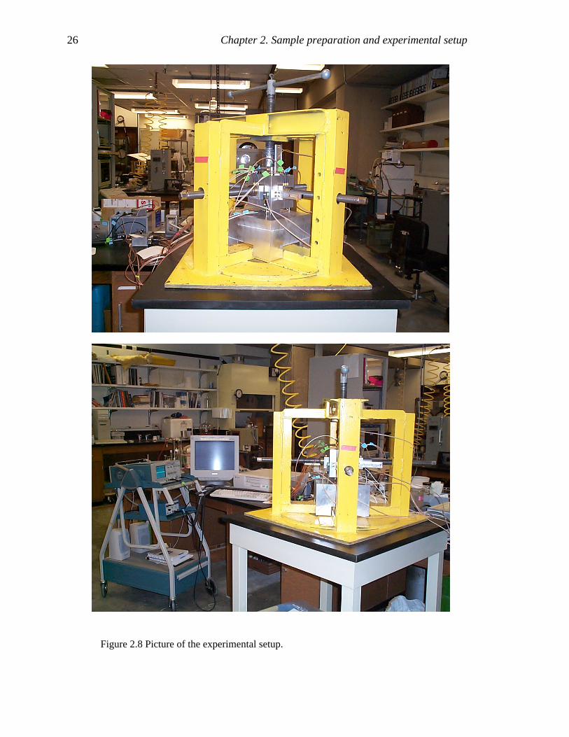
26 Chapter 2. Sample preparation and experimental setup
Figure 2.8 Picture of the experimental setup.

Chapter 2. Sample preparation and experimental setup 27
2.3.1 Stress distribution within the samples Stress distributions in granular materials are not well understood. Attempts have
made to simulate these stresses using different models that depend on varying system
conditions (de Gennes, 1999; Geng et al., 2001). For example, a 2D granular sample
under a point load results in fairly uniform stresses close to the load, and stress “chains”
(spatially inhomogeneous stresses) that split with distance at packing defects (Claudin et
al., 1998; Bouchaud et al., 2001; Geng et al., 2001). For this problem, Bouchaud et al.
(2001) modeled local stress chain splitting at packing defects using local hyperbolic
equations in the approximation of the chain-mean-free-path (λ, mean length with
continuous stress chains) larger than the grain radius (a). They calculated the average of
the vertical stresses on several statistically identical numerical samples. The dimensions
of these samples were LxL. For samples with large length (L) compared with λ, that is,
L >> λ >> a, (2.3)
they showed that this stress average as a function of the horizontal distance is similar to
the elastic solution (elliptical equation) of a normal line load on a semi-infinite region,
For the polyaxial apparatus and most of the present samples (except GB3),
L ≈ 7.5cm. (2.4)
a = grain-size/2 ≈ (0.05/2)cm. (2.5)
λ: unknown. (2.6)
⇒ L/a ≈ 300 >> 1 . (2.7)
Hence, experimental conditions presented in this thesis can be considered to be of large
length scale, and comparable with the model of Bouchaud et al. (2001).
In addition to the stress distribution analysis, I estimated that the error in the stress
measurements at the loading platens was around 3%, using that
)l2(AF
AF
2 ∆+∆
=σ∆ (2.8)

28 Chapter 2. Sample preparation and experimental setup
where F is the force measured in the dial gauge, ∆F is the force error measurement, A is
the area of the loading piston, and ∆l is the error in the length measurements.
(a)
(b)
Figure 2.9 (a) Normal load over AB in a semi-infinite medium in 2D; (b) 2D
sketch of the polyaxial apparatus cell and loading platens.
3.82 cmA
l = 7.5 cm
h cell
platen
B
0
Z
XA B
3.82 cmA
l = 7.5 cm
h cell
platen
B
0
Z
XA B
A B
σPz
0
Z
XA B
σPz
0
Z
X

Chapter 2. Sample preparation and experimental setup 29
2.3.2 Stress analysis in an uniaxial strain test I now present an estimate of the stress distribution inside the sample cell for the case
of uniaxial strain, which is discussed in Chapter 5. In the uniaxial strain test, samples are
placed in the polyaxial cell and an axial stress is applied via the top platen in the Z-
direction, and the horizontal platens are held fixed, at approximately zero displacement.
As illustrated in Figure 2.9, the vertical stress is applied to the sand sample through the
platen, having area 22
5.11282.3 cmA =⎟
⎠⎞
⎜⎝⎛= π . If the total force applied by the piston is Fz,
then the stress immediately under the platen is approximately
PzPz A/F=σ . (2.9)
This platen stress Pzσ is the stress that is recorded as the “Applied Stress, σ z” throughout
this thesis.
As shown in Figure 2.9, the platen is smaller than the internal cross sectional area of
the sample in the cell, 22Cell cm5.7A = , or 2.0)5.7/5.11(A/A 2CellPz == . Therefore, the
distribution of stress applied to the top of the sample is likely to be quite heterogeneous –
large under the platen, but falling off to much smaller values along portions of the top of
the sample that are not in contact with the platen. According to Saint-Venant’s principle,
a distribution of force statistically equivalent to zero applied on a surface of an elastic
material produces negligible strains at distances larger than the linear scale of the force
distribution (Fung, 1965). By this principle, we expect that the stress distribution in an
elastic material should become more spatially homogeneous away from the loading
surface. The question to address is how we can quantitatively estimate these stresses.
I followed the lead of Bouchaud et al. (2001) and choose an elastic analysis. To
model the problem of a normal force localized near the center of the sample top, and zero
displacement conditions along the sample sides, I used the exact solution for a doubly
periodic normal stress applied to the surface of a half space (Fung, 1965). The vertical
compressive stress zσ at z = 0 is with the form

30 Chapter 2. Sample preparation and experimental setup
⎥⎥⎦
⎤
⎢⎢⎣
⎡⎟⎟⎠
⎞⎜⎜⎝
⎛ π⎟⎟⎠
⎞⎜⎜⎝
⎛ π+⎟
⎟⎠
⎞⎜⎜⎝
⎛ π⎟⎟⎠
⎞⎜⎜⎝
⎛ πσ=σ
yx1'
y'x
ooz Lycos
Lxcosa
Lycos
Lxcosa (2.10)
where ao and a1 are coefficients describing the non-uniformity of the applied stress, Lx
and Ly are the sample lengths measured from the platen center in X and Y, respectively,
and 'xL and '
yL are distances far away from the sample, such as yx'x
'x L,LLL >>≈ . In
general, the vertical and lateral solutions (Fung, 1965) are
⎥⎥⎦
⎤
⎢⎢⎣
⎡⎟⎟⎠
⎞⎜⎜⎝
⎛ π⎟⎟⎠
⎞⎜⎜⎝
⎛ π++⎟
⎟⎠
⎞⎜⎜⎝
⎛ π⎟⎟⎠
⎞⎜⎜⎝
⎛ π+σ=σ −− cz
yx1
z'c'y
'x
ooz eL
ycosL
xcos)cz1(aeL
ycosL
xcos)z'c1(a , (2.11)
]eL
ycosL
xcos)cz2(ca
eL
ycosL
xcos)cz''2'('c
a[
cz
yx
22221
z'c'y
'x
2222o
ox
−
−
⎟⎟⎠
⎞⎜⎜⎝
⎛ π⎟⎟⎠
⎞⎜⎜⎝
⎛ πα+νβ−α−
+⎟⎟⎠
⎞⎜⎜⎝
⎛ π⎟⎟⎠
⎞⎜⎜⎝
⎛ πα+νβ−α−σ=σ
, (2.12)
where 'xL
' π=α , '
yL' π=β , 22 '''c β+α= , which go to zero for yx
'x
'x L,LLL >>≈ ,
xLπ
=α , yL
π=β , 22c β+α= , and ν is the Poisson’s ratio. For the effect of this
analysis, I assumed ν=0.4 as this value corresponds to a soft material.
If ao=1 and a1=0, then the applied stress is uniform; this could occur if the sand
behaved as a liquid, flowing perfectly up and around the platen and transmitting the
platen stress to the upper stationary surface of the sample cell. On the other hand, if
ao=0.5 and a1=0.5, then the stress is maximum in the middle and goes to zero at the
edges, exhibiting more of a solid behavior. We have no direct measure of the stress
distribution within the aluminum sample; however, we use this latter assumption and that
yx'x
'x L,LLL >>≈ in the analysis below:

Chapter 2. Sample preparation and experimental setup 31
⎥⎥⎦
⎤
⎢⎢⎣
⎡⎟⎟⎠
⎞⎜⎜⎝
⎛ π⎟⎟⎠
⎞⎜⎜⎝
⎛ π+
σ≈σ
yx
oz L
ycosL
xcos12
(2.13)
Because of the symmetry associated with the periodicity of the problem, the
horizontal displacements are exactly zero along the planes xLx ±= and yLy ±= .
Therefore, the periodic solution for the half-space automatically gives the uniaxial strain
solution for the region ;Ly;Lx yx << . Furthermore, within this region, the applied
stress has a maximum of oz σ=σ at the center of the sample top, x = y = z = 0, and falls
off smoothly to zero at the sample edges xLx ±= ; yLy ±= ; 0z = . The resulting vertical
and lateral stresses are shown in Figures 2.10 and 2.11 for the case 1o =σ , and ao=0.5
and a1=0.5, and in Figure 2.12 and 2.13 for the case case 1o =σ , and ao=0.75 and
a1=0.25.
For the case 1o =σ , and ao=0.5 and a1=0.5, in the vertical stress solution (Figure
2.10), we see that the stress heterogeneity falls off rapidly with distance from the sample
top, and approaches an average value
2/oavgz σ≈σ − (2.14)
The total applied force in Z is
Cellavgz
Cello
yx
ozz
A2/A
dxdyL
ycosL
xcos12
dAF
−σ=σ=
⎥⎥⎦
⎤
⎢⎢⎣
⎡⎟⎟⎠
⎞⎜⎜⎝
⎛ π⎟⎟⎠
⎞⎜⎜⎝
⎛ π+
σ=σ= ∫∫∫∫
. (2.15)
Therefore the apparent platen stress in Z is

32 Chapter 2. Sample preparation and experimental setup
( )( )PCellavgz
PCello
PzPz
A/A2/A/A
A/F
−σ=σ=
=σ (2.16)
Therefore, the average vertical stress in the sample is
( )Pz
CellPPzavgz2.0
A/Aσ≈
σ=σ − (2.17)
Note that if the applied stress were uniform across the top of the entire sample, i.e.,
ao=1 and a1=0, then we would get a very different result appropriate for a liquid:
Pzavgz σ≈σ − .
In the horizontal stress solution (Figure 2.11), we see that the stress heterogeneity
falls off quickly with distance from the top reaching an average horizontal stress (σx-avg).
Thus, we can take the apparent platen stress in X as avgxPx −σ≈σ . In addition, at the
sample sides, the stress near the horizontal platens is
( )
Pz
Pz
avgz
ox
18.0*2.0*2*45.0
245.045.0
σ≈σ≈
σ≈σ≈σ
− (2.18)
This ratio depends on the apparent “pseudo-Poisson’s ratio” assumed for the sample,
which in this case was taken as 0.4. A Poisson’s ratio of 0.2 (more appropriate for
consolidated sandstone) would give a value Pox 14.035.0 σ≈σ≈σ for the sample sides.
Finally, we can estimate the relation between the apparent stress ratio PzPx / σσ and
the internal sample stress ratio avgzavgx / −− σσ :
Pz
Px
avgz
avgx
2.0 σσ
≈σσ
−
− . (2.19)

Chapter 2. Sample preparation and experimental setup 33
For the case 1o =σ , and ao=0.75 and a1=0.25 (Figure 2.12 and 2.13), which
corresponds to a material that behaves more like a liquid, and using the previous
procedure, I found that,
Pz
Px
avgz
avgx
39.0 σσ
≈σ
σ
−
− , (2.20)
with Pzoavgz 3.075.0 σ≈σ≈σ − , and Pzox 4.065.0 σ≈σ≈σ . Hence, equation 2.19 gives an
“estimated true stress” lower bound that is for the extreme case of assuming that the sand
behaves as an elastic soft solid. Equation 2.20 gives an “estimated true stress” assuming
that the sand can behave close to a liquid. Neither of these two assumptions solutions
presents the definitive solution of this problem as it is yet not clear what model describes
better the real stress behavior in the sand under the polyaxial apparatus conditions. With
these solutions, I only intend to give an approximate stress range inside the samples
related with the “measured stress”. If this analysis is correct, then the internal stress
anisotropy is smaller than the measured platen stress anisotropy.
In summary,
• The measured horizontal stress, as indicated by the horizontal platens and load
cells, appears to be a good estimate of the true sample horizontal stress, for the
uniaxial stain problem.
• On the other hand, if we assume that the material behaves more or less like an
elastic solid, then the true vertical stress in the sample is smaller than the
measured vertical platen stress by a factor of approximately 2.0A/A CellP = .
• If we assume that the material behaves more or less close to a liquid, then the
true vertical stress in the sample is smaller than the measured vertical platen
stress by a factor of approximately 0.3.
• If the sample behaves as a perfect liquid, then the true vertical stress in the
sample equals the measured vertical platen stress.
We emphasize that throughout this dissertation, the values of stress in most tables and
graphs should be interpreted as “measured stress”, defined by load cell force divided by

34 Chapter 2. Sample preparation and experimental setup
platen area. We occasionally apply the above corrections, and these will be referred to as
“estimated true stress.” Future improvements to this kind of analysis would include a
finite-element analysis of an elasto-plastic sample.
Figure 2.10 Estimated vertical stress σz for the uniaxial strain problem, using the elastic solution of a doubly periodic normal stress applied to the surface of a half space (ao=a1=0.5, Poisson’s ratio = 0.4). Profiles at bottom show the stress along the sample top (red line) and horizontally across the middle of the sample (blue line). Profile at the right shows the stress vertically through the sample center. Heavy bars along the colored stress map indicate platens.
Z
X

Chapter 2. Sample preparation and experimental setup 35
Figure 2.11 Estimated horizontal stress σx for the uniaxial strain problem, using
the elastic solution of a doubly periodic normal stress applied to the surface of a half space (ao=a1=0.5, Poisson’s ratio = 0.4). Profiles at bottom show the stress along the sample top (red) and horizontally across the middle of the sample (blue). Profile at the right shows the stress along the right and left edges of the cell. Heavy bars along the colored stress map indicate platens.
2.3.3 Stress analysis in a quasi-hydrostatic stress experiments
We can make a similar estimate of the relation between measured platen stress and
internal sample stress for the quasi-hydrostatic test. In the quasi-hydrostatic stress test,
samples are placed in the polyaxial cell and approximately equal forces are applied via
the platens in each of the three principal directions. I use a principle of superposition to
extend the results of the previous analysis. The procedure is as follows
- Apply an increment of platen stress PzA σ=σ in the Z-direction. From the previous
analysis for ao=a1=0.5, the internal sample stresses in the Z and X directions are
approximately Az 2.0 σ≈σ and Ax 18.0 σ≈σ
- Superimpose an increment of platen stress Aσ in the X-direction and Y-direction.
This adds an increment of Ayx 36.0 σ≈σ+σ to both the platen and the internal sample
stress in the Z-direction.
Z
X

36 Chapter 2. Sample preparation and experimental setup
Szz; PR= 0.4
-1 -0.5 0 0.5 1
0
0.2
0.4
0.6
0.8
1
1.2
1.4
1.6
1.8
2 0
0.1
0.2
0.3
0.4
0.5
0.6
0.7
0.8
0.9
1
00.5
10.6 0.8 1
Figure 2.12 Estimated vertical stress σz for the uniaxial strain problem, using the
elastic solution of a doubly periodic normal stress applied to the surface of a half space (ao=0.75, a1=0.25, Poisson’s ratio = 0.4). Profiles at bottom show the stress along the sample top (red line) and horizontally across the middle of the sample (blue line). Profile at the right shows the stress vertically through the sample center.
- Therefore, the total stress on the Z-platen in the quasi-hydrostatic test is
AAAqPz 36.118.0*2 σ≈σ+σ≈σ and the internal sample stress is
AAAq
avgz 56.018.0*22.0 σ≈σ+σ≈σ −
- So the ratio of cumulative internal sample stress to cumulative stress on the platen
for ao=a1=0.5 is:
( ) qPz
qPz
qavgz 4.036.1/56.0 σ≈σ≈σ − . (2.21)
Using the same procedure for ao=0.75 and a1=0.25, ratio of cumulative internal sample
stress to cumulative stress on the platen is
( ) qPz
qPz
qavgz 6.08.1/1.1 σ≈σ≈σ − . (2.22)
Z
X

Chapter 2. Sample preparation and experimental setup 37
Sxx; PR= 0.4
-1 -0.5 0 0.5 1
0
0.2
0.4
0.6
0.8
1
1.2
1.4
1.6
1.8
2 0
0.1
0.2
0.3
0.4
0.5
0.6
0.7
0.8
0.9
1
00.5
10.4 0.6 0.8
Figure 2.13 Estimated horizontal stress σx for the uniaxial strain problem, using
the elastic solution of a doubly periodic normal stress applied to the surface of a half space (ao=0.75, a1=0.25, Poisson’s ratio = 0.4). Profiles at bottom show the stress along the sample top (red) and horizontally across the middle of the sample (blue). Profile at the right shows the stress along the right and left edges of the cell.
In summary, we estimate that the internal quasi-hydrostatic stress is approximately
0.4 and 0.6 of the stress, for an elastic solid and elastic more like a liquid, respectively;
indicated by the load cell force divided by platen area. Again, this assumes that the sand
behaves as an elastic material with Poisson’s ratio 0.4. A future improvement would be
to repeat the analysis with a finite element simulation of an elasto-plastic material.
2.3.4 Experimental Stress Configurations In this dissertation, results from three loading configurations will be shown:
Hydrostatic pressure. In this case, cylindrical samples are jacketed with flexible
tygon tubing, and the pressure is applied in a hydrostatic cell via pressurized oil pushing
uniformly against the jacket.
Quasi-Hydrostatic stress. In this case, the cubic samples are placed in the polyaxial
cell and approximately equal forces are applied via the platens in each of the three
principal directions.
Z
X

38 Chapter 2. Sample preparation and experimental setup
Uniaxial Strain. In this case, the cubic samples are placed in the polyaxial cell. An
axial stress is applied in the Z-direction, and the horizontal platens are held fixed, at
approximately zero displacement.
2.4 Sample and apparatus setup guide The procedure for setting up the samples and apparatus is as follows:
1. Transducers, o-rings, and frame should be clean.
2. Distances from the middle hole, S1, in the transducer to the contact side (dtx, drx,
dty, dry) are measured with a caliper and glass lamina (as reference). That is, dtx,y, drx,y =
dtx,y, drx,y - lamina thickness (Figure 2.14).
3. O-rings are greased and placed on the transducers. Fine o-rings are used for the
receivers in X and Y, and for the transmitter in Z. One thick o-ring (outer side) and one
fine o-ring (inner side) are used for the transmitters in X and Y, and for the receiver in Z.
4. The bottom transducer (Z-receiver) with the o-rings is fixed to the frame using
silicone between the transducer and the frame. The silicone must be allowed to cured,
which takes about 24 hours, before the sample is put inside.
Figure 2.14 Measurement of transducer lengths to be used in the total length of
the samples.
5. Molasses is spread on the transducers.
dtx,y or drx,y
lamina
P S1 S2
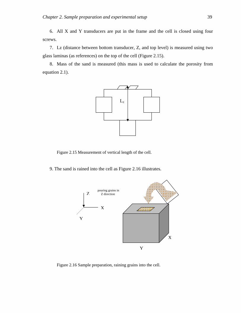
Chapter 2. Sample preparation and experimental setup 39
6. All X and Y transducers are put in the frame and the cell is closed using four
screws.
7. Lz (distance between bottom transducer, Z, and top level) is measured using two
glass laminas (as references) on the top of the cell (Figure 2.15).
8. Mass of the sand is measured (this mass is used to calculate the porosity from
equation 2.1).
Figure 2.15 Measurement of vertical length of the cell.
9. The sand is rained into the cell as Figure 2.16 illustrates.
Figure 2.16 Sample preparation, raining grains into the cell.
Lz
Y
X
Z
Y
X
pouring grains in Z direction

40 Chapter 2. Sample preparation and experimental setup
10. Dx and Dy (distance between transmitter and receiver transducers using middle
hole S1 for each direction X and Y) are measured and the measurements are repeated two
times, that is, the final horizontal lengths of the sample are lx,y = Dx,y – (dtx,y + drx,y )
(Figure 2.17).
Figure 2.17 Measurement of the horizontal lengths of the sample, lx and ly.
11. Space between the sand and top of the cell (∆lz) is measured with the internal part
of the caliper, that is, the length in Z direction is lz = Lz – ∆lz (Figure 2.18)
Figure 2.18 Measurement of vertical length of the sample, ∆lz.
12. The cell is closed with the Z-receiver transducer on top of the cell.
13. The cell is put in the platform.
14. All potentiometers are screwed in the following order:
lx,y
Dx,y
dtx,y drx,y
∆lz lz Lz

Chapter 2. Sample preparation and experimental setup 41
Potentiometer # 1: Z-receiver (bottom)
Potentiometer # 2: Z-transmitter (top)
Potentiometer # 3: X-transmitter (X load cell)
Potentiometer # 4: X-receiver
Potentiometer # 5: Y-transmitter (Y load cell)
Potentiometer # 6: Y – receiver
15. Potentiometer readings are measured to take the initial lengths.
16. The load nuts are placed as near to center as possible.
17. The samples are loaded with the initial stress, and allowed to equilibrate for eight
to ten hours before velocity measurements are made. This equilibration period is repeated
for each loading step until the force read-out stabilizes (1.5 hours in loading and 0.5 hour
in unloading). Deformation measurements are made immediately after loading and at
stabilized stresses to control and study mechanical behavior between waiting times.
18. After velocity, stress, and deformation measurements, the cell with the sample is
removed from the apparatus platform, the cell is opened, and the platens and o-rings are
cleaned, using pressurized air.
2.5 References
Baxter, J., Tuzun, U., Heyes, D., Hayati, I., and Fredlund P., 1998, Stratification in
poured granular heaps: Nature, 391, 136.
Becker, E., 1982, Velocity of sound, CRC Handbook of Chemistry and Physics, pp. E-45,
CRC Press, Inc, Florida.
Bouchaud, J. P., Claudin, P., Levine, D., and Otto, M., 2001, Force chain splitting in
granular materials: a mechanism for large-scale pseudo-elastic behavior: The
European Physical Journal E, 4, 451-457.
Cizeau, P., Makse, H. A., and Stanley, E., 1999, Mechanisms of granular spontaneous
stratification and segregation in two-dimensional silos: Physical Review E, 59, 4408-
4421.

42 Chapter 2. Sample preparation and experimental setup
Claudin, P., Bouchaud, J. P., Cates, M. E., and Wittmer, 1998, Models of stress
fluctuations in granular media: Physical Review E, 57, 4441-4457.
Cristescu, N. D., and Hunsche, U., 1998, Time effects in rocks mechanics, pp. 55-58,
John Wiley & Sons Ltd., West Sussex, England.
de Gennes, P. G., 1999, Granular matter: a tentative view: Reviews of Modern Physics,
71, S374-S382.
Fioravante, V., and Capoferri, R., 2001, On the use of multi-directional piezoelectric
transducers in triaxial testing: Geotechnical Testing Journal, 24, 243-255.
Fretti, C., Lo Presti, D. C. F., and Pedroni, S., 1995, A pluvial deposition method to
reconstitute well-graded sand specimens: Geotechnical Testing Journal, 18, 292-298.
Fung, Y.C., 1965, Foundations of Solid Mechanics, pp. 195-197, Prentice-Hall,
Englewood Cliffs, NJ.
Geng, J., Howell, D., Longhi, E., and Behringer, R. P., 2001, Footprints in sand: the
response of a granular material to local perturbations: Physical Review Letters, 87,
355061-355064.
Jaeger, J. C., and Cook, N. G. W., 1979, Fundamentals of Rock Mechanics, pp. 13, 285-
302, 387, 425-440, Chapman and Hall, London.
Jaeger, H. M., Nagel, S. R., and Behringer, R. P., 1996, Granular solids, liquids, and
gases: Reviews of Modern Physics, 68, 1259-1273.
Kopperman, S. E., 1982, Effect of state of stress on velocity of low-amplitude
compression waves propagating along principal stress directions in sand: M. Sc.
thesis, The University of Texas at Austin, pp. 21-71, 191-215, Austin, TX.
Makse, H. A., Gland, N., Johnson, D. L., Schwartz, L. M., 1999, Why effective medium
theory fails in granular materials: Physical Review Letter, 83, 5070-5073.
Rad, N. S., and Tumay, M. T., 1985, Factors affecting sand specimen preparation by
raining: Geotechnical Testing Journal, 10, 31-37.
Santamarina, J. C., and Cascante, G., 1996, Stress anisotropy and wave propagation: a
micromechanical view: Canadian Geotechnical Journal, 33, 770-782.
Santamarina, J. C., 2001, Soils and waves: John Wiley & Sons LTD, pp. 276-278,
Chichester, England.

Chapter 2. Sample preparation and experimental setup 43
Sih, G., C., 1981, Experimental evaluation of stress concentration and intensity factors,
pp.2-4, Martinus Nijhoff Publishers, Netherlands.
Yin, H., 1993, Acoustic velocity and attenuation of rocks; isotropy, intrinsic anisotropy,
and stress-induced anisotropy: Ph.D. thesis, Stanford University, pp. 118-178,
Stanford, CA.
Zimmer, M., 2003, Thesis: in preparation.
Zeng, X., 1999, Stress-induced anisotropic Gmax of sands and its measurements: Journal
of Geotechnical and Geoenvironmental Engineering, 125, 741-749.

44 Chapter 2. Sample preparation and experimental setup

45
Chapter 3 Comparative study of velocities under hydrostatic pressure and quasi-hydrostatic stress in sands 3.1 Introduction
Laboratory measurements of acoustic velocity in sands are most often made under
hydrostatic pressure (Domenico, 1997; Zimmer et al., 2002; Wang, 2002). Stresses in the
lithosphere are generally non-hydrostatic and anisotropic (Sinha and Kostek, 1996,
Winkler et al., 1994, Zoback and Zoback, 2000). Although Mavko et al. (1995) suggested
a method for rocks to predict stress-induced velocity anisotropy from hydrostatic lab
measurements of Vp and Vs, a similar prediction for sands has not yet been
demonstrated.
Domenico (1977) measured acoustic velocities under hydrostatic pressure in a sand
and in glass beads of similar grain size and porosity; the resulting velocity, pore volume,
porosity, and pore compressibility as functions of pressure for dry and brine-saturated
samples led to a better understanding of unconsolidated formations. Wang (2002)
measured the velocity anisotropy of sands, shales, and rocks under hydrostatic pressure in
the laboratory, and developed a relation to estimate Vp anisotropy from Vs anisotropy
and vice versa. However, since all of these correlations were derived under hydrostatic
pressure, they are difficult to extrapolate to in situ stress, as will be illustrated in Chapter
5 for stress anisotropy in sands using a polyaxial cell.
A question that arises at this point is how the observations in a polyaxial cell are
related with standard velocity measurements in a hydrostatic pressure. In this chapter, I
study Vp measured under hydrostatic pressure and quasi-hydrostatic stress conditions in a
sand, and I find that they are not the same. Here, I use “hydrostatic stress” to describe
pressurizing a sample surrounded by oil, and “quasi-hydrostatic stress” to describe a load

46 Chapter 3. Comparative study of velocities under hydrostatic and quasi-hydrostatic…
applied mechanically in three orthogonal directions with pistons; “isotropic stress” is
when the compressive stress in all directions is the same. The quasi-hydrostatic stress is
called isotropic (non-hydrostatic isotropic stress) when the three principal stresses are the
same. I explain my procedure for applying isotropic stress using a polyaxial apparatus.
When I examine velocities in three perpendicular directions as functions of stress, I find
that Vp under hydrostatic pressure is higher than Vp measured under non-hydrostatic
isotropic stress. Although making an appropriate correction of measured to “true” stress
(describe in Chapter 2) reduces the difference. I observe velocity anisotropy associated
with intrinsic anisotropy in the sands even under this isotropic stress. In addition, I find
that the loading order in the polyaxial apparatus affects the velocity anisotropy for
repetitive stress cycles.
The organization of this chapter is as follows: (1) the experimental tests to measure
Vp in sands under hydrostatic pressure, and quasi-hydrostatic stress are described; (2)
results on depositional anisotropy are shown; (3) results on strain and porosity are
explained; and (4) results on Vp under hydrostatic pressure and quasi-hydrostatic stress
are presented and compared.
3.2 Experimental setup and procedure I used a hydrostatic and a polyaxial apparatus to compare compressional velocity
(Vp) and strain (ε) under hydrostatic pressure and quasi-hydrostatic stress in a sand. I
implemented a test called “quasi-hydrostatic” which consists of creating isotropic stress
(σx ≈ σy ≈ σz) in the polyaxial apparatus. In other words, it is a non-hydrostatic, isotropic
stress test.
3.2.1 Quasi-hydrostatic stress test For the quasi-hydrostatic stress test, I used the polyaxial apparatus described in
Chapter 2. In this apparatus, the sample is contained in an aluminum cell that can be
loaded compressionally in three perpendicular directions with pistons.
In the quasi-hydrostatic stress test, the same compressive stress was applied in all
three directions, σz ≈ σx ≈ σy. I loaded (and unloaded) the samples by successively
incrementing in small steps σz, then σx, and following with σy to reach final σ for that
velocity and strain measurement. To check the possible influence of the loading

Chapter 3. Comparative study of velocities under hydrostatic and quasi-hydrostatic… 47
sequence on the results, I also changed the order of loading increments to σx, σy, and then
σz. At each step, I followed the same order of loading (and unloading) and allowed the
stresses to stabilize until the force gauge gave a constant value for one hour (and half an
hour), before making the acoustic measurements. Vp and strain in the X, Y, and Z
direction (Vpx, Vpy, and Vpz, and εx, εy, and εz, respectively) were measured. Unless
otherwise indicated, the stresses shown for the quasi-hydrostatic stress experiments are
the “measured stresses” given by the load cell force divided by the platen area. In a few
cases I apply a single correction as obtained in Chapter 2.
3.2.2 Hydrostatic test For the hydrostatic pressure tests, I used an oil-loading pressure vessel (Vanorio et al.,
2002). The sample is contained in a cylindrical tygon jacket and is subjected to a
confining pressure applied with oil. Vp and strain in the axial direction (εz) were
measured, no radial Vp and ε measurement were possible, because of limitations of this
apparatus.
To be consistent with the polyaxial test, the confining pressure steps were the same as
in the quasi-hydrostatic stress test and the sample was allowed to stabilize (for an average
of about half an hour) before making the acoustic measurements. The principal frequency
of the piezoelectric crystals for P-wave generation was 1 MHz in both apparatus. Because
of attenuation, the recorded waveforms had frequencies about one order of magnitude
lower (see Chapter 5).
3.2.3 Samples and sample preparation I used the Santa Cruz sand described in Chapter 2, which is a beach sand with an
average grain size of 0.25 mm. The grain size analysis was made by sieving, and the
grain density was measured using a pycnometer (measured by Zimmer, 2003). This sand
shows natural stratification when it is poured (Figure 3.1a). It has been referred to as
“unstable” configuration, as any singular rolling grain causes grain flow in the rest of the
sandpile (Cizeau et al., 1999). This stratification has been observed in different mixtures
of granular materials (Makse et al., 1997; Baxter et al., 1998; Cizeau et al, 1999) and is
discussed in more detailed in Chapter 4.

48 Chapter 3. Comparative study of velocities under hydrostatic and quasi-hydrostatic…
I made four samples, one for the hydrostatic pressure test, HNS, and three for the
quasi-hydrostatic stress test QNS1, QNS2, and SCR. All samples were poured in the
vertical direction (Z) creating the natural stratification characteristic of this sand. The
HNS sample was poured into a cylindrical rubber jacket for the hydrostatic apparatus and
the QNS samples were poured into the aluminum cell for the polyaxial apparatus. SCR
was first poured and then rotated 90° around the X-axis, i.e. Z and Y directions were
exchanged in the final configuration (Figure 3.1b). For the hydrostatic apparatus, a
rotated sample similar to SCR was not possible, again because of limitations of the setup.
Figure 3.1 (a) Natural stratification shown in the poured sand: the black line shows one of the layers naturally formed. (b) Rotated sand around X direction, equivalent to the SCR sample: the black lines show mainly interpreted features. (Pictures taken in a transparent container outside the aluminum cell).
Average porosity for all samples was 0.47, with a sample-to-sample variation lower
than 2% (Table 3.1). All samples were measured room dry during the loading and
unloading of three stress cycles up to measured stress of 40 bars. QNS1 was used for the
Z→X→Y loading order, and QNS2 for the X→Y→Z loading order. Table 3.1
summarizes the samples and applied tests (see Table 2.1 for more detailed sample
characteristics).
Z
Y Y (former Z)
Z (former Y)

Chapter 3. Comparative study of velocities under hydrostatic and quasi-hydrostatic… 49
Table 3.1 Sample summary
Sample name Test Loading order φ
HNS Hydrostatic 0.46
QNS1 Quasi-hydrostatic Z→X→Y 0.48
QNS2 Quasi-hydrostatic X→Y→Z 0.47
SCR Quasi-hydrostatic Z→X→Y 0.47
3.3 Results
3.3.1 Depositional anisotropy In this section, I show how Vp anisotropy revealed depositional anisotropy under
quasi-hydrostatic stress. A more detailed study on the depositional anisotropy is
presented in Chapter 4.
Figure 3.2 and Figure 3.3 show Vp as a function of the mean stress,
σ = (σz + σx + σy) /3, for QNS1, QNS2, and SCR for the loading path in the first stress
cycle. Figure 3.2 displays the velocity anisotropy in QNS1 and QNS2 due to its
depositional anisotropy. Vpz, which was in the direction perpendicular to the layering,
was lower than Vpx and Vpy. This is the typical result in a VTI medium, Vp along the
bedding layers is layer than Vp perpendicular to layers. A change in the order of loading
(QNS2) produced similar results, as shown in Figure 3.2b. In this case Vpx was slightly
higher than Vpy (5%), which indicates a slight effect of the order of loading on Vp. The
development of this difference and the velocity anisotropy of QNS1 and QNS2 is
discussed in section 3.4.3 and section 3.5.3.
To test whether the sample had depositional anisotropy, I measured velocity in a cell
that was rotated after grains were rained in, SCR (Figure 3.3). Velocity in the unchanged
horizontal direction Vpx remained high, i.e., waves in the X-direction continue to
propagate alomh horizontal layers after rotation. However, velocities in the exchanged
vertical (Vpz) and horizontal (Vpy) directions were now equal and lower than Vpx. As
shown in Figure 3.1, the Y-Z rotation causes flow in the Y-Z plane and tends to destroy
the layering in the plane. This result supports the idea that Vp is sensitive to the internal

50 Chapter 3. Comparative study of velocities under hydrostatic and quasi-hydrostatic…
structure (depositional anisotropy) in the samples, giving in SCR a more complicated
behavior due to the complexity of its depositional history (Figure 3.1b).
0
200
400
600
800
1000
1200
0 10 20 30 40σ (bars)
Vp
(m/s
)
VhVpzVpxVpy
(a)
0
200
400
600
800
1000
1200
0 10 20 30 40σ (bars)
Vpz
(m/s
)
VhVpzVpxVpy
(b)
Figure 3.2 Quasi-hydrostatic stress and hydrostatic pressure test. Compressional
velocity as a function of compressive stress for (a) QNS1 and HNS, and (b) QNS2 and HNS, during the loading path for the first stress cycle. (Open circles, squares, and triangles denote QNS1 Vpz, Vpx, and Vpy, respectively. Closed circles represent HNS velocity in the Z direction, Vh). Vpx, Vpy, and Vpz lower than 0.5 bar are not plotted as their error bars are in the order of the velocity anisotropy.
HNS QNS1
HNS QNS2

Chapter 3. Comparative study of velocities under hydrostatic and quasi-hydrostatic… 51
0
200
400
600
800
1000
1200
0 10 20 30 40σ (bars)
Vp
(m/s
) VhVpz VpxVpy
Figure 3.3 Quasi-hydrostatic stress and hydrostatic pressure test. Compressional
velocity as a function of mean stress for SCR and HNS for the loading path in the first stress cycle. (Open circles, squares, and triangles denote SCR Vpz, Vpx, and Vpy, respectively. Closed circles represent HNS velocity in the Z direction, Vh). Vpx, Vpy, and Vpz lower than 0.5 bar are not plotted as their error bars are in the order of the velocity anisotropy.
3.3.2 Strain and porosity Figure 3.4 shows strain in the Z direction (εz), normalized to unity at the largest
applied stress, as a function of the mean stress for the naturally stratified samples (HNS,
QNS1, and QNS2) in the loading path of the first stress cycle. We see that εz, which was
perpendicular to the layers, was different in each of these samples. It seems that the strain
was more affected than Vp by the different loading patterns, even for hydrostatic pressure
or quasi-hydrostatic stress in a different loading order. εz-σ in QNS1 matched better with
εz-σ in HNS during unloading, and εz-σ in QNS2 matched better with εz-σ in HNS during
loading. εz at mean stresses lower than 4 bars seems to be more related to grain
rearrangement, which was most likely affected by the type of loading. That is, εz in HNS
showed gradual compression, εz in QNS1 (Z→X→Y) showed the highest compression at
the first loading step, and εz in QNS2 (X→Y→Z) initially showed extension. This
extension can be due to the loading order: the two first loading directions were in X and
Y, compressing the sample in the XY plane and extending it in the Z direction, the
HNS
SCR

52 Chapter 3. Comparative study of velocities under hydrostatic and quasi-hydrostatic…
loading in Z at very low stresses was not enough to compress the sample in that direction.
The extension in Z decreased with stress until 4 bars after which only compression started
to be observed. Avoiding these initial rearrangements in the samples due to the different
loading mechanisms, I analyze in more detail εz at mean stresses higher than 4 bars as
follows.
Figure 3.5a shows εz as a function of mean stress for stresses higher than 4 bars in all
samples. We see the same trend of εz-σ for the samples measured in the polyaxial
apparatus, and a slightly different trend for the HNS sample. The strain for SCR was
higher than for QNS samples, which we suspect was due to the depositional anisotropy
(Figure 3.1b) rather than the slight difference in porosity. It seems that the depositional
anisotropy in SCR was such that the remaining layers in the Z direction (originally Y
direction) were more unstable in this direction than the horizontal layers in QNS. The
strain for SCR at the highest mean stress was much higher (0.076) than for the lower
stresses in the loading and unloading paths. This value was not included in the fit as it
was an isolated peak. In addition, there was a slight difference in εz between QNS1 and
QNS2, most likely as a consequence of the porosity, which varied by 1% between these
samples.
Figure 3.5b shows εz as a function of the axial strain in HNS, εz(HNS), for mean
stress higher than 4 bars in the loading path of first stress cycle. We see a correlation
between the strain measured under hydrostatic pressure and quasi-hydrostatic stresses.
This correlation is a consequence of all samples in the quasi-hydrostatic stress test having
similar trends (Figure 3.5a). εz-εz(HNS) for QNS1 and QNS2 were more similar than εz-
εz(HNS) for SCR. This result is as we expect, because QNS1 and QNS2 had the same
depositional anisotropy. Consequently, these correlations suggest a gradual increment of
strain with mean stress with a connection between hydrostatic pressure and quasi-
hydrostatic stress tests that is slightly affected by the type of sample.

Chapter 3. Comparative study of velocities under hydrostatic and quasi-hydrostatic… 53
(a)
(b)
(c) Figure 3.4 Quasi-hydrostatic stress and hydrostatic pressure test. Strain in the Z
direction (εz) as a function of the mean stress for all natural stratified samples: (a) HNS (open circles), (b) QNS1 (close circles), and (c) QNS2 (close squares). Straight lines denote loading paths and dashed lines denote unloading paths.
-0.8
-0.4
0.0
0.4
0.8
1.2
0 10 20 30 40
σ (bars)
εz (n
orm
aliz
ed)
HNS
-0.8
-0.4
0.0
0.4
0.8
1.2
0 10 20 30 40
σ (bars)
εz (n
orm
aliz
ed)
QNS1
-0.8
-0.4
0.0
0.4
0.8
1.2
0 10 20 30 40
σ (bars)
εz (n
orm
aliz
ed)
QNS2

54 Chapter 3. Comparative study of velocities under hydrostatic and quasi-hydrostatic…
(a)
(b)
Figure 3.5 Quasi-hydrostatic stress and hydrostatic pressure test. Strain in the Z
direction, εz, as a function of (a) mean stress, and (b) axial strain in HNS, for the loading path in the first stress cycle at stresses higher than 4 bars. (Open circles, squares, and triangles represent QNS1, QNS2, and SCR, respectively; close circles represent HNS. SCR strain at the highest stress presented a peak value that was not included in the fit. Black straight lines represent linear fits and gray straight line is the linear function εz = εz (HNS)).
R2 = 0.93
R2 = 0.92
R2 = 0.72
R2 = 0.990.00
0.01
0.02
0.03
0.04
0 10 20 30 40σ (bars)
ε z
QNS1QNS2SCRHNS
R2 = 0.97
R2 = 0.94
R2 = 0.74
0.00
0.01
0.02
0.03
0.04
0.000 0.001 0.002 0.003 0.004 0.005 0.006
εz (HNS)
εz
QNS1QNS2SCR
εz = εz (HNS)

Chapter 3. Comparative study of velocities under hydrostatic and quasi-hydrostatic… 55
Figure 3.6, Figure 3.7, and Figure 3.8 show how the strain evolved with stress in three
perpendicular directions for QNS1, QNS2, and SCR respectively. We notice that the
highest initial displacement in the QNS samples was inelastic and in the X direction.
QNS1, for which the order of loading was Z→X→Y, had the major initial displacement
in εx, followed by εz and εy. In addition, εx was compressive while εy was extensive. On
the other hand, QNS2, in which the order of loading was X→Y→Z, had the major initial
displacement in εx followed by εy and εz, which is in the same order as loading, with
higher displacement in the XY plane (εx and εy). Furthermore, SCR had the major initial
displacement in εz followed by εx and εy, which is also in the same order as loading, with
higher displacement in the Z direction also inelastic. For this last sample, with an initial
stratification rotated around the ZY plane, the remaining layers were in the Z direction.
These results suggest that the major initial displacement was higher in the first loading
direction on the plane of the layers.
In summary (Table 3.2), εx was similar in both QNS samples, εy in QNS1 was lower
than εy and higher than εz in QNS2, and finally εz in QNS1 was higher than εz and lower
than εy in QNS2. εx, εy, and εz were different in SCR relative to QNS because of their
different depositional fabric.
Figure 3.9 shows Vp as a function of porosity in HNS, QNS1, and QNS2 for three
stress cycles. In the hydrostatic pressure test, HNS, only one direction (Z) of Vp and
strain was measured (due to the apparatus limitations). I found that HNS had no
significant change in porosity for the three cycles. In this porosity calculation the radial
deformation was not includes but if we assume the same axial and radial displacement,
we found that the change in porosity in HNS is more significant (Figure 3.9a). This result
indicates that isotropic deformation in the samples can lead to a miscalculation of
porosity changes if only the axial deformation is measured. In addition, a possible
explanation of no porosity change between the cycles might be the elastic resistance of
the jacket to the pressure at these low pressures. In contrast, the quasi-hydrostatic stress
tests, QNS1 and QNS2, had significant porosity change in and between the three stress
cycles.

56 Chapter 3. Comparative study of velocities under hydrostatic and quasi-hydrostatic…
(a) (b) (c)
Figure 3.6 Quasi-hydrostatic stress test. Strain as a function of compressive stress in QNS1 for the (a) first stress cycle, (b) second stress cycle, and (c) third stress cycle.
-0.02
-0.01
0
0.01
0.02
0.03
0.04
0.05
0.06
0.07
0.08
0 10 20 30 40 50
σ (bars)
ε
zxy
-0.02
-0.01
0.00
0.01
0.02
0.03
0.04
0.05
0.06
0.07
0.08
0 10 20 30 40 50
σ (bars)
ε
zxy
-0.02
-0.01
0.00
0.01
0.02
0.03
0.04
0.05
0.06
0.07
0.08
0 10 20 30 40 50
σ (bars)
ε
zxy

Chapter 3. Comparative study of velocities under hydrostatic and quasi-hydrostatic… 57
(a) (b) (c)
Figure 3.7 Quasi-hydrostatic stress test. Strain as a function of compressive stress in QNS2 for the (a) first stress cycle, (b) second stress cycle, and (c) third stress cycle.
-0.02
-0.01
0
0.01
0.02
0.03
0.04
0.05
0.06
0.07
0.08
0 10 20 30 40 50
σ (bars)
ε
zxy
-0.02
-0.01
0.00
0.01
0.02
0.03
0.04
0.05
0.06
0.07
0.08
0 10 20 30 40 50
σ (bars)
ε
zxy
-0.02
-0.01
0.00
0.01
0.02
0.03
0.04
0.05
0.06
0.07
0.08
0 10 20 30 40 50
σ (bars)
ε
zxy

58 Chapter 3. Comparative study of velocities under hydrostatic and quasi-hydrostatic…
0
0.01
0.02
0.03
0.04
0.05
0.06
0.07
0.08
0 10 20 30 40 50σ (bars)
ε
zxy
(a)
0.00
0.01
0.02
0.03
0.04
0.05
0.06
0.07
0.08
0 10 20 30 40 50σ (bars)
ε
zxy
(b)
0.00
0.01
0.02
0.03
0.04
0.05
0.06
0.07
0.08
0 10 20 30 40 50σ (bars)
ε
zxy
(c)
Figure 3.8 Quasi-hydrostatic stress test. Strain as a function of compressive stress in SCR for the (a) first stress cycle, (b) second stress cycle, and (c) third stress cycle.

Chapter 3. Comparative study of velocities under hydrostatic and quasi-hydrostatic… 59
(a)
(b)
(c) Figure 3.9 Vp as a function of porosity, φ, for (a) hydrostatic pressure test, HNS,
and quasi-hydrostatic stress test: (b), QNS1, and (c) QNS2.
0
200
400
600
800
1000
1200
0.430 0.435 0.440 0.445 0.450 0.455 0.460 0.465 0.470 0.475 0.480φ
Vpz
(m/s
)
Cycle 1Cycle 2Cycle 3
0
200
400
600
800
1000
1200
0.430 0.435 0.440 0.445 0.450 0.455 0.460 0.465 0.470 0.475 0.480φ
Vp (m
/s)
VpzVpyVpy
Cycle 1Cycle 3 Cycle 2
0
200
400
600
800
1000
1200
0.430 0.435 0.440 0.445 0.450 0.455 0.460 0.465 0.470 0.475 0.480φ
Vp (m
/s) VpzVpxVpy
Cycle 1Cycle 3 Cycle 2
Φ using only axial deformation
Φ assuming radial deformation = axial deformation

60 Chapter 3. Comparative study of velocities under hydrostatic and quasi-hydrostatic…
Table 3.2 Summary of strain and velocity measurements under quasi-hydrostatic
stress and hydrostatic pressure.
Sample Loading order
Strain (ε) Vp εz : εz(HNS) Vpz : Vp(HNS)
QNS1 (stratified)
Z→X→Y εx >εz>εy Vpx≈Vpy>Vpz εz>εz(HNS) Vpz<Vp(HNS)
QNS2 (stratified)
X→Y→Z εx >εy >εz Vpx≈Vpy>Vpz εz≥ εz(HNS) Vpz<Vp(HNS)
SCR (initially stratified and then rotated)
Z→X→Y εz >εx >εy Vpx>Vpy≈Vpz εz>>εz(HNS) Vpz<Vp(HNS)
3.3.3 Vp under hydrostatic pressure and quasi-hydrostatic stress Figure 3.10 and Figure 3.11 show Vp as a function of compressive stress for QNS1
and QNS2, respectively, and HNS for three stress cycles. There was no significant
increment of Vp on Vp hysteresis between these cycles. Nevertheless, in the last cycle for
QNS1, Vpz was slightly closer to Vpy, and Vpx was slightly separated from Vpy. This
result might indicate that for this loading order (Z→X→Y) the original depositional
anisotropy could change after many loading cycles. For QNS2, Vpx separated from Vpy
after the second stress cycle.

Chapter 3. Comparative study of velocities under hydrostatic and quasi-hydrostatic… 61
(a)
(b)
(c)
Figure 3.10 Quasi-hydrostatic stress and hydrostatic pressure test. Compressional velocity as a function of compressive stress in QNS1 for (a) first stress cycle, (b) second stress cycle, and (c) third stress cycle.
0
200
400
600
800
1000
1200
0 10 20 30 40 50σz,x,y (bars)
Vp (m
/s)
VpzVpxVpyVh
0
200
400
600
800
1000
1200
0 10 20 30 40 50σz,x,y (bars)
Vp
(m/s
)
VpzVpxVpyVh
0
200
400
600
800
1000
1200
0 10 20 30 40 50σz,x,y (bars)
Vp
(m/s
)
VpzVpxVpyVh

62 Chapter 3. Comparative study of velocities under hydrostatic and quasi-hydrostatic…
(a) (b) (c)
Figure 3.11 Quasi-hydrostatic stress and hydrostatic pressure test. Compressional
velocity as a function of compressive stress in QNS2 for (a) first stress cycle, (b) second stress cycle, and (c) third stress cycle.
0
200
400
600
800
1000
1200
0 10 20 30 40 50σz,x,y (bars)
Vp
(m/s
)
VpzVpxVpyVh
0
200
400
600
800
1000
1200
0 10 20 30 40 50σz,x,y (bars)
Vp
(m/s
)
VpzVpxVpyVh
0
200
400
600
800
1000
1200
0 10 20 30 40 50
σz,x,y (bars)
Vp
(m/s
)
VpzVpxVpyVh

Chapter 3. Comparative study of velocities under hydrostatic and quasi-hydrostatic… 63
Figure 3.2a (or Figure 3.9) and Figure 3.2b (or Figure 3.10) show Vp in the Z
direction for HSN (Vh) as a function of pressure, and compared with the QNS1 and
QNS2 velocities, respectively. As revealed by the graphs, Vh, which was perpendicular
to the layers, was higher than Vpx, Vpy, and Vpz in QNS1 and QNS2. We can also see
that the Vh-pressure curve increased faster than the Vpz-stress curve for QNS1 and
QNS2 at stresses lower than 22 bars, and increased slower at stresses higher than 22 bars.
Figure 3.3 shows Vh as a function of the pressure, compared with the SCR velocities
in the loading path of the first stress cycle. As for QNS1 and QNS2 in Figure 3.2, Vh was
also higher than Vpz. The Vh-pressure curve and Vpz-stress curve for SCR increased
equally at stresses lower than 22 bars, and the Vh-pressure curve increased slower than
this Vpz-stress curve at stresses higher than 22 bars. Nevertheless, results on SCR only
illustrate how different Vp can be when measured under hydrostatic pressure and quasi-
hydrostatic stress, in addition to the effects of different internal structure or depositional
anisotropy.
Table 3.3 summarizes the velocity comparison between the samples under hydrostatic
pressure and quasi-hydrostatic stress. It is clear that velocities measured under hydrostatic
pressure are not equal to velocities measured under quasi-hydrostatic stress fields, even
for an approximately isotropic stress field with the same depositional anisotropy (HNS,
QNS1, and QNS2).
Table 3.3 Comparison of velocities measured under quasi-hydrostatic stress and
hydrostatic pressure.
Velocities Sample
Same direction Different direction100*
VVV
h
zh − 100*V
VV
h
xh − *
HNS
QNS1 QNS2 Vh > Vpz Vh > Vpx ≈Vpy 27% 7% - 12%
HNS
SCR Vh > Vpz Vpx ≥ Vh >Vpy 8% - 12% 4%
* 100*
VVV
h
yh − is similar .

64 Chapter 3. Comparative study of velocities under hydrostatic and quasi-hydrostatic…
3.4 Discussion
3.4.1 Depositional anisotropy The velocity anisotropy detected in QNS1 and QNS2 (Figure 3.2) is consistent with
the natural stratification shown in Figure 3.1a. The velocity anisotropy detected in SCR
(Figure 3.3) deviates from a VTI (vertical transverse isotropic) anisotropy. For instance,
Figure 3.1b shows that the packing of SCR is more complex than QNS. For SCR, it
seems that some of the original layers formed during pouring became more curved after
the rotation, because of gravity induced flow. In a simple way, this can explain why Vpz
and Vpy are lower than Vpx. Vpy is measured in the perpendicular direction to the
layers, Vpz is perpendicular to the layer, and Vpx is in the direction that is persistently
parallel to layers.
Vh is higher than Vpz for the two packings, QNS and SCR. It is 27% higher for QNS,
and 8-12% for SCR at measured stresses up to 40 bars (Table 3.2). This difference
between QNS and SCR indicates that the divergence between velocities measured under
hydrostatic pressure and quasi-hydrostatic stress conditions can be also affected by the
depositional anisotropy of the sands. Therefore, to extrapolate hydrostatic lab Vp to non-
hydrostatic in situ Vp, it is necessary to know the direction of the velocity measurement
with respect to the geological formation anisotropy.
3.4.2 Strain and porosity The strain appears to be more affected by the type of loading than is Vp, especially at
stresses lower than 4 bars. Figure 3.4 presents a good example of different ε-σ behavior
for different type of loading, and Figure 3.6 and Figure 3.7 present a good example of
how a different order of loading gives a different order of displacement. This strain
behavior for different loading order also displayed a higher mobility in the plane (XY) of
the depositional layers, or unstable layers, than in the perpendicular direction Z.
3.4.3 Vp under hydrostatic pressure and quasi-hydrostatic stress Figure 3.9, and Figure 3.10 reveal that Vpz was always lower than Vh for all samples
with same depositional anisotropy, and both figures present the same trend Vpz-σ. This
result could be affected by the stress inside the polyaxial cell. However, I estimated the
stress distribution in the cell in Chapter 2, using the elastic solution of a doubly periodic

Chapter 3. Comparative study of velocities under hydrostatic and quasi-hydrostatic… 65
normal stress applied to the surface of a half space. For the quasi-hydrostatic stress test, I
found that the measured stress in the platens was different from the internal sample stress
(estimated true stresses). The ratio of the estimated true stress, qavgz−σ , and the measured
stress, qPzσ , was q
Pzq
avgz 4.0 σ≈σ − and qPz
qavgz 6.0 σ≈σ − for an elastic soft solid and an elastic
more like a liquid, respectively. If we re-scale the measured stresses with this estimated
correction, we still obtain that Vh is higher than Vpz, but the relative difference is much
lower than taking the velocities at the measured stresses (Figure 3.12). In addition, the
relative difference between Vh and Vpz at the measured stresses is around 27% (Table
3.2), while the relative difference between Vh and Vpz at the estimated true stress is
around 10%, and only around 4% for the higher stresses. This means that if this estimated
correction is proper, hydrostatic pressure and quasi-hydrostatic stress test are equivalent.
Figure 3.12 Compressional velocity measured in the quasi-hydrostatic stress test
as a function of compressional velocity measured in the hydrostatic pressure test. Black symbols correspond to the velocities at the measured stresses (platens stress), red symbols correspond to the velocities at the estimated true stresses (internal sample stress) assuming the case of an elastic soft solid, which correction is around 40% in the measured stresses ( q
Pzq
avgz 0.4σσ ≈− ).
In addition, I found that Vp anisotropy was affected by the order of loading for more
than two stress cycles. In the first stress cycle there was no significant difference in the
Vp anisotropy for the different loading orders. Furthermore, Vh was always higher than
Vpz.
400
600
800
1000
1200
400 600 800 1000 1200Vh (m/s)
Vpz
(m/s
)
QNS1QNS2QNS1(0.4)QNS2(0.4)

66 Chapter 3. Comparative study of velocities under hydrostatic and quasi-hydrostatic…
3.5 Conclusions The velocity anisotropy under isotropic stress revealed depositional anisotropy in the
sand samples. That is, Vp anisotropy under isotropic stress corroborates that depositional
anisotropy can be detected with Vp sands. Moreover, Vp measured under hydrostatic
pressure (Vh) was higher than Vp measured under quasi-hydrostatic stress in the sand, for
the same depositional anisotropy and similar isotropic stress. The difference between
hydrostatic Vp and quasi-hydrostatic stress Vp might be due to border effects as the
solution of a half space surface with an applied periodic normal stress suggests. In
addition, strain was more affected by different loading than Vp. The strain behavior with
stress displayed a higher mobility in the direction of the depositional layers than in the
perpendicular direction. Finally, the order of loading in the quasi-hydrostatic stress test
affected the original depositional anisotropy (revealed in Vp anisotropy) in the sand for
more than two consecutive stress cycles.
3.6 References Baxter, J., Tuzun, U., Heyes, D., Hayati, I., and Fredlund P., 1998, Stratification in
poured granular heaps, Nature, 391, 136.
Cizeau, P., Makse, H. A., and Stanley, E., 1999, Mechanisms of granular spontaneous
stratification and segregation in two-dimensional silos, Physical Review E, 59, 4408-
4421.
Domenico, S. N., 1977, Elastic properties of unconsolidated porous sand reservoirs:
Geophysics, 42, 1339-1368.
Jaeger, J. C., and Cook, N. G. W., 1979, Fundamentals of Rock Mechanics, Halsted
Press, New York.
Makse, H. A., Havlin, S., King, P., and Stanley, H. E., 1997, Spontaneous stratification in
granular mixtures: Nature, 386, 379-381.
Mavko, G., Mukerji, T., Godfrey, N., 1995, Predicting stress-induced velocity anisotropy
in rocks: Geophysics, 60, 1081-1087.
Sinha, B. K. and Kostek, S., 1996, Stress-induced azimuthal anisotropy in borehole
flexural waves: Geophysics, 61, 1899-1907.

Chapter 3. Comparative study of velocities under hydrostatic and quasi-hydrostatic… 67
Vanorio, T., Prasad, M., Nur, A., and Patella, D., 2002, Ultrasonic velocity measurements
in volcanic rocks: correlation with microtexture: Geophysical Journal International,
149, 22 - 36.
Wang, Z., 2002, Seismic anisotropy in sedimentary rocks, part 2: laboratory data:
Geophysics, 67, 1423-1440.
Winkler, K., Plona, T., Hsu, J., and Kostek, S., 1994, Effects of borehole stress
concentrations on dipole anisotropy measurements: 64th Annual International
Meeting, Society of Exploration Geophysicists, Expanded Abstracts, 1136-1138.
Zimmer, M., Prasad, M., and Mavko, G., 2002, Pressure and porosity influences on Vp-
Vs ratio in unconsolidated sands: The Leading Edge, 21, 180-183.
Zoback, M. D., and Zoback M. L., State of stress in the Earth’s lithosphere, IASPEI
Encyclopedia of Seismology, in press, 2000.

68 Chapter 3. Comparative study of velocities under hydrostatic and quasi-hydrostatic…

69
Chapter 4 Intrinsic anisotropy in soft sediments and its seismic potential 4.1 Introduction
In nature there is stratification, as a form of intrinsic anisotropy, in many sedimentary
structures such as river deposits, streams, fan deltas, estuarine and tidal deposits, beaches
and shelves, slope and deep sea deposits, and eolian sand dunes. Intrinsic anisotropy is
the result of preferential orientation of the sediment grains and pores that can be created
by sediment composition, grain size and shape, and deposition. Intrinsic anisotropy in
sediments may be enhanced by crystal structures and can be very complex, especially
when clay is present. For this study, I avoid issues of compositional differences and focus
on stratification due to deposition, as revealed by poured sediments.
In poured grains, it has been found that deposition speed and grain size and shape
determine packing. Makse et al. (1997) and Cizeau et al. (1999) have shown that natural
stratification occurs in poured granular mixtures for specific combinations of grain sizes
and shapes, for example, for a mixture of large rough and small rounded grains.
However, Baxter et al. (1998) reported that natural stratification also depends on
deposition speed: mixtures of the same grain shape and various grain sizes resulted in
stratification for a relative low speed deposition. On the other hand, poured grains have
shown segregation for mixtures of large rough grains and small rounded grains, and
mixtures of the same grain size and different shapes. Therefore, segregation and
stratification may affect the texture of sediment mixtures, or packings. Figure 4.1 shows a
qualitative explanation of grain sizes and shape conditions for segregation and
stratification, as presented by Cizeau et al. (1999).

70 Chapter 4. Intrinsic anisotropy in sediments and its seismic potential
(a)
(b)
(c) Figure 4.1 Segregation and stratification according to Cizeau et al. (1999). (a)
Segregation: same grain shape (repose angle) and different grain size (larger grains go on the bottom). (b) Segregation: different grain shape (lower repose angle grains go on the bottom) and same grain size. (c) Stratification (competition of (a) and (b) effects): larger grains with higher repose angle.
In Chapter 3, I found that P-wave velocity anisotropy for the quasi-hydrostatic stress
also is affected by the intrinsic anisotropy in sands corroborating previous work (Jiang et
al., 1997; Tai and Sadd, 1997; Chen et al., 1998; Fioravante and Capoferri, 2001). This
result led me to investigate more the intrinsic anisotropy and P-wave velocity anisotropy
in the sands and glass beads in this chapter. It is not well understood how segregation and
stratification might affect P-wave velocity, or acoustic velocities in general. Acoustic
velocities change with elastic properties of the constituents, and are often used to
discriminate different lithologies. They are also sensitive to stress anisotropy (Nur and
Simmons, 1969; Yin, 1993; Tai and Sadd, 1997; Chen et al., 1998). If compressional

Chapter 4. Intrinsic anisotropy in sediments and its seismic potential 71
velocity (most commonly used in situ) responds to sediment packings, this can help to
reveal how velocity is related to internal sedimentary structure. Pan and Dong (1999)
proposed a method to detect texture with acoustical velocities that uses optimization, but
it works well only if it has the right micro-features input: normal distribution of
anisotropic contact, shape and orientation of the grains, average radius of the grains, void
ratio, stiffness ratio, shear modulus, and frictional angle. The purpose of this chapter is
twofold: (1) to explore whether compressional velocity, Vp, is sensitive to packing in
poured sediments, and (2) to measure whether an intrinsic velocity anisotropy exists in
poured sediments under isotropic stress, before looking at stress-induced anisotropy.
In this chapter, I present a study of intrinsic P-wave anisotropy focusing on
stratification of poured sediments. I describe the experimental procedure to detect the
intrinsic anisotropy in Vp in sand and glass bead samples. I then offer a method to
determine textural anisotropy with the spatial autocorrelation function. This method uses
the spatial autocorrelation function and its variation with direction to characterize the
stratification texture from images of the samples. To determine if there is a relation
between Vp and the textural anisotropy, I compare velocity anisotropy and the spatial
autocorrelation function. Finally, I find that velocity anisotropy reveals internal packing.
4.2 Methods To study Vp and its relation to packing, I used the polyaxial apparatus described in
Chapter 2 to measure Vp and strain (ε) in three perpendicular directions in sand and glass
bead samples. I also used a code written by Dr. Tapan Mukerji to calculate the anisotropy
ratio based on the autocorrelation function of the sample images.
4.2.1 Experimental procedure In the experiments, I used a polyaxial apparatus (Chapter 2) and attempted to apply
the same compressive stress in all three directions, σz ≈ σx ≈ σy. I loaded (and unloaded)
the samples by successively incrementing σz, then σx, and following with σy (Z→X→Y).
I did not need to vary this order of loading, because, as discussed in Chapter 3, the order
of loading does not significantly affect the velocity measurements in the first loading
cycle. Vp and ε were measured in the Z, X, and Y directions; the measured components
were Vpz, Vpx, and Vpy, and εz, εx, and εy, respectively. At each step, I followed the

72 Chapter 4. Intrinsic anisotropy in sediments and its seismic potential
same order of loading (and unloading), and the stresses were allowed to stabilize before
making the acoustic measurements. Stabilization was determined when the load value
became steady in time.
I used Santa Cruz sand (QNS1 and SCR), which is a beach sand with an average
grain size of 0.25 mm, and glass beads GB1, GB2, and GB3 with grain size 0.25-0.3 mm,
0.5-0.6 mm, and 2.794-3.327 mm, respectively. See Chapter 2 and Table 2.1 for detailed
description of these samples.
All samples were poured vertically (in the Z direction) into the aluminum cell in the
polyaxial apparatus. I prepared two different samples with the sand, which were also
used in Chapter 3: QNS1, which was only poured and SCR, which was initially poured
and then rotated 90° around the X-axis; that is, the. Z and Y directions were exchanged in
the final configuration. In addition, I made replicas of the samples in transparent plastic
containers and took photographs of them, since I cannot take pictures through the opaque
apparatus cell. As illustrated in Figure 4.2, images for the XZ (back and front), ZY (back
and front), and XY (top) planes were taken (Figure 4.2).
4.2.2 Method for textural anisotropy interpretation To help with the interpretation of the images, I used a code made by Dr. Tapan
Mukerji that calculates the autocorrelation function of images at azimuth angles between
0° to 180°. This code first finds the 2D Fourier transform of the image; second, it applies
the autocorrelation theorem, which says that a function times its complex conjugate is
equal to the modulus of its Fourier transform; third, it finds the autocorrelation function
for each angle from 0° to 180°; fourth, it finds the lags at an autocorrelation function of e-
1 for each angle, which is called correlation length; and finally, it calculates the
anisotropy ratio (AR), defined as the ratio between the maximum and the minimum
correlation length. The median correlation length is also estimated. In addition, a
perpendicular anisotropy ratio, AR', defined as the ratio between the correlation length at
0° and 90° was calculated.

Chapter 4. Intrinsic anisotropy in sediments and its seismic potential 73
Figure 4.2 Image sketch example for ZX and XY planes (plastic container replica
of QNS1).
I processed the images in the ZX (back and front), ZY (back and front), and XY (top)
planes for all the samples. I used the following steps: (1) sample image was selected for
the chosen plane taking care avoid edges of the image close to the container walls, (2) a
gray-scale image was made, (3) the gray image histogram was equalized (to transform
the gray intensity values to a flat histogram), and (4) the histogram was filtered to find a
reasonable median correlation length of at least two grains, to detect the general features
as layers, and finally (5) the anisotropy ratio and the angles of the autocorrelation
anisotropy were calculated. To validate this process, I also created a synthetic image of a
hexagonal 2D packing and used plane images of a laminated consolidated shale (Figure
4.3), which present well defined anisotropies: hexagonal and transversal isotropy,
respectively.
front
back
top
X
Z
Y
XY

74 Chapter 4. Intrinsic anisotropy in sediments and its seismic potential
Figure 4.3 Different plane views of the laminate shale sample (with the
lamination direction in the XY plane).
4.3 Results
4.3.1 Experimental lab results. Velocity anisotropy Figure 4.4 shows compressional velocities as functions of the mean applied stress, σ.
Vp was not the same in all three directions; i.e. there was velocity anisotropy in all the
samples. In QNS1 (Figure 4.4a), Vpx and Vpy were equal and higher than Vpz as
expected for a horizontal layered TI medium. In SCR (Figure 4.4b), Vpz and Vpy were
similar but lower than Vpx. This result indeed reveals differences in intrinsic anisotropy
between the two sand samples, which was expected, since SCR was disturbed by
rotation.
ZX ZY
XY (top) XY (bottom)

Chapter 4. Intrinsic anisotropy in sediments and its seismic potential 75
(a) (b)
(c) (d)
(e) Figure 4.4 Quasi-hydrostatic stress test. Vp versus mean stress, σ = σz +σx
+σy /3, where σz ≈ σx ≈ σy. Vpz, Vpx, and Vpy are the Vp velocities in the Z, X, and Y axes. Sand samples are plotted a different scale than glass bead samples. (a) QNS1, (b) SCR, (c) GB1, d) GB2, (e) GB3. (Open circles, squares, and triangles denote Vpz, Vpx, and Vpy, respectively). Vpx, Vpy, and Vpz lower than 0.5 bar are not plotted as their error bars are in the order of the velocity anisotropy.
0
200
400
600
800
1000
1200
0 10 20 30 40σ (bars)
Vp (m
/s) Vpz
VpxVpy
0
200
400
600
800
1000
1200
0 10 20 30 40σ (bars)
Vp
(m/s
)
VpzVpxVpy
0
400
800
1200
1600
0 10 20 30 40σ (bars)
Vp (m
/s)
VpzVpxVpy
0
400
800
1200
1600
0 10 20 30 40σ (bars)
Vp (m
/s)
VpzVpxVpy
0
400
800
1200
1600
0 10 20 30 40σ (bars)
Vp (m
/s)
VpzVpxVpy

76 Chapter 4. Intrinsic anisotropy in sediments and its seismic potential
In general, Vpz was lower than Vpx and Vpy for the glass bead samples. In GB1
(Figure 4.4c), all three velocities were similar. In GB2 (Figure 4.4d), the velocity
anisotropy behavior was similar to QNS1. Finally, in GB3 (Figure 4.4e), all three
perpendicular velocities were different, with a change in Vpx and Vpy at 32 bars, which
corresponded to a reported crack sound during loading. In all cases, however, Vpz was
smaller than Vp in the other directions.
4.3.2 Textural anisotropy interpretation In the next section, I first describe the appearances of the sample images and then
estimate their textural anisotropy using their autocorrelation functions.
4.3.2.1 Qualitative sample description based on the images QNS1 showed natural stratification, as can be seen in Figure 4.2, and was mentioned
in Chapter 2. Roughly horizontal layers (parallel to the XY plane) are spontaneously
created every time this sand is poured. These layers were more notable in the ZY plane
than in the ZX plane. This stratification can be explained using Cizeau et al. (1999): the
more rounded (lower repose angle) and smaller grains are inserted in layers with the
rougher and larger grains since the two effects shown in Figure 4.1a and 4.1b are
competing; and Baxter et al. (1998): relative low speed of deposition, which was
consistently used in all samples.
In contrast, the resulting packing for SCR was more complex, as grains slipped
during rotation because of gravity, and the original stratification was broken. Figure 4.5a
shows an image of SCR in the ZY plane, perpendicular to the rotation axis X. It seems
that some of the original layers became more curved after the rotation because of gravity
in the ZY plane.
GB1 (with a standard deviation of grain size of 0.04) showed light segregation in the
ZX and ZY planes, and an almost homogenous texture in the XY plane. GB2 (with a
standard deviation of 0.07) seemed to have a high level of segregation on the ZX and ZY
planes, and a random appearance on the XY plane. This segregation can be explained
with the segregation mechanism shown in Figure 4.1a, and must be due to the slight
difference in the range of the grain sizes in the samples, which was greater in the GB2, as
shown by its higher standard deviation.

Chapter 4. Intrinsic anisotropy in sediments and its seismic potential 77
In contrast, GB3 (with a standard deviation of 0.38) showed some layers on the
bottom and on the vertical edges combined with some diagonally aligned beads on the
ZY and ZX planes. On the XY plane, this sample also showed aligned beads on the walls,
and a general orientation to the center. This sample showed very different behavior
during the preparation because of the size of its beads; they sprang electrostatically
toward the walls of the container, so that gravity was probably not the only influence on
packing.
So far my description of texture in images has been qualitative. Next, I attempted to
quantify the textural anisotropy using the spatial autocorrelation function and its variation
with direction.
(a) (b)
(c) (d)
Figure 4.5 SCR sample image in the ZY plane: (a) sample picture, (b) gray
image, (c) equalized image (b), and (d) equalized and filtered image.
Santa Cruz sand - rotated (X1) gray
equalized filtered
Y
Z
(former Z)
(former Y)
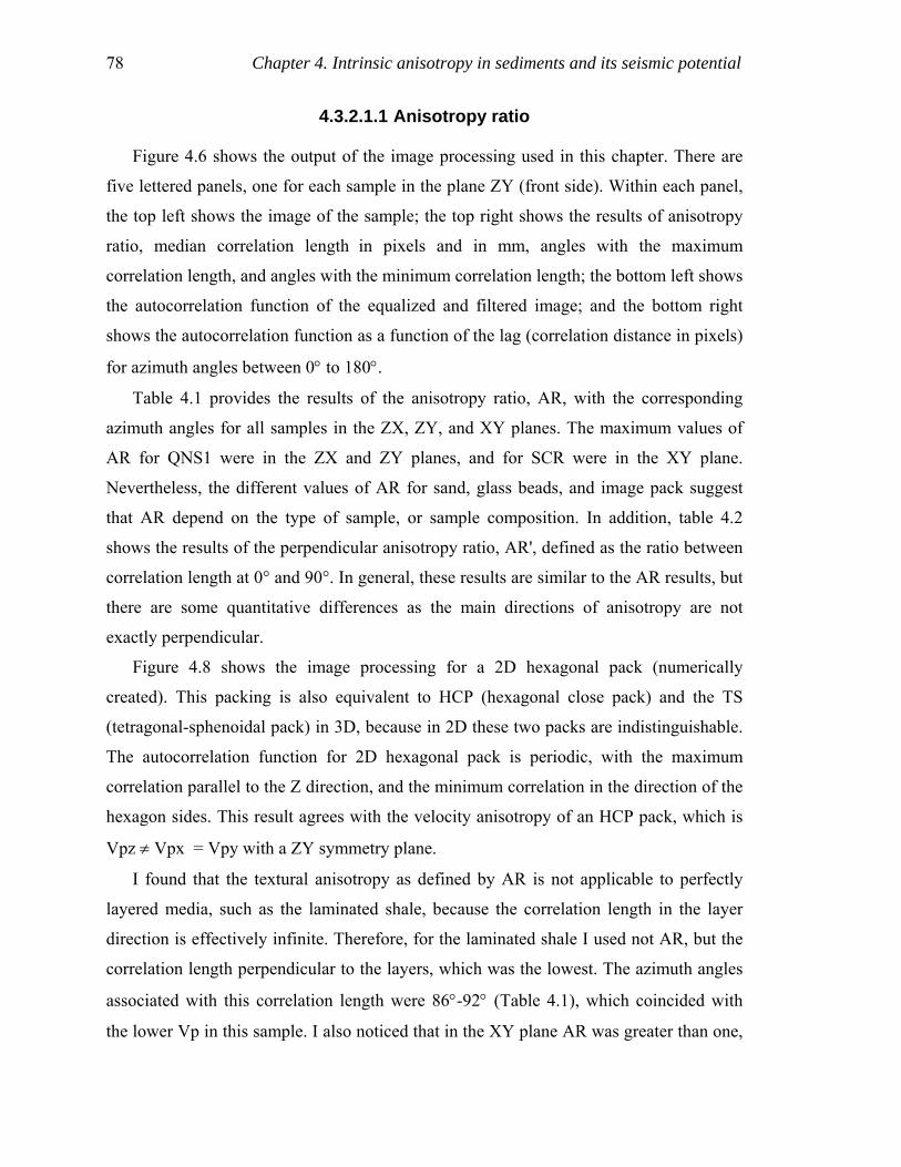
78 Chapter 4. Intrinsic anisotropy in sediments and its seismic potential
4.3.2.1.1 Anisotropy ratio
Figure 4.6 shows the output of the image processing used in this chapter. There are
five lettered panels, one for each sample in the plane ZY (front side). Within each panel,
the top left shows the image of the sample; the top right shows the results of anisotropy
ratio, median correlation length in pixels and in mm, angles with the maximum
correlation length, and angles with the minimum correlation length; the bottom left shows
the autocorrelation function of the equalized and filtered image; and the bottom right
shows the autocorrelation function as a function of the lag (correlation distance in pixels)
for azimuth angles between 0° to 180°.
Table 4.1 provides the results of the anisotropy ratio, AR, with the corresponding
azimuth angles for all samples in the ZX, ZY, and XY planes. The maximum values of
AR for QNS1 were in the ZX and ZY planes, and for SCR were in the XY plane.
Nevertheless, the different values of AR for sand, glass beads, and image pack suggest
that AR depend on the type of sample, or sample composition. In addition, table 4.2
shows the results of the perpendicular anisotropy ratio, AR', defined as the ratio between
correlation length at 0° and 90°. In general, these results are similar to the AR results, but
there are some quantitative differences as the main directions of anisotropy are not
exactly perpendicular.
Figure 4.8 shows the image processing for a 2D hexagonal pack (numerically
created). This packing is also equivalent to HCP (hexagonal close pack) and the TS
(tetragonal-sphenoidal pack) in 3D, because in 2D these two packs are indistinguishable.
The autocorrelation function for 2D hexagonal pack is periodic, with the maximum
correlation parallel to the Z direction, and the minimum correlation in the direction of the
hexagon sides. This result agrees with the velocity anisotropy of an HCP pack, which is
Vpz ≠ Vpx = Vpy with a ZY symmetry plane.
I found that the textural anisotropy as defined by AR is not applicable to perfectly
layered media, such as the laminated shale, because the correlation length in the layer
direction is effectively infinite. Therefore, for the laminated shale I used not AR, but the
correlation length perpendicular to the layers, which was the lowest. The azimuth angles
associated with this correlation length were 86°-92° (Table 4.1), which coincided with
the lower Vp in this sample. I also noticed that in the XY plane AR was greater than one,
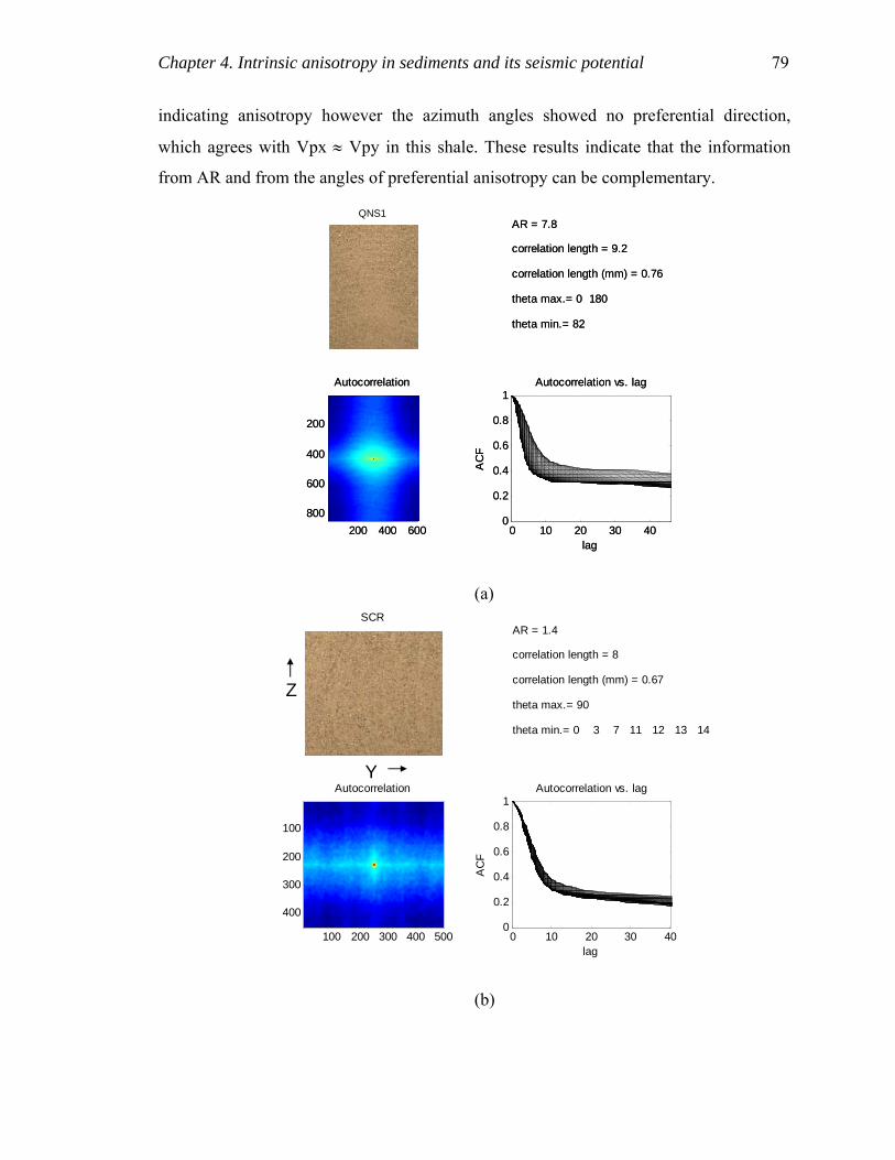
Chapter 4. Intrinsic anisotropy in sediments and its seismic potential 79
indicating anisotropy however the azimuth angles showed no preferential direction,
which agrees with Vpx ≈ Vpy in this shale. These results indicate that the information
from AR and from the angles of preferential anisotropy can be complementary.
(a)
(b)
SCR
Autocorrelation
100 200 300 400 500
100
200
300
400
0 10 20 30 400
0.2
0.4
0.6
0.8
1
lag
AC
F
Autocorrelation vs. lag
AR = 1.4
correlation length = 8
correlation length (mm) = 0.67
theta max.= 90
theta min.= 0 3 7 11 12 13 14
Y
Z
SCS
Autocorrelation
200 400 600
200
400
600
8000 10 20 30 40
0
0.2
0.4
0.6
0.8
1
lag
AC
F
Autocorrelation vs. lag
AR = 7.8
correlation length = 9.2
correlation length (mm) = 0.76
theta max.= 0 180
theta min.= 82
QNS1SCS
Autocorrelation
200 400 600
200
400
600
8000 10 20 30 40
0
0.2
0.4
0.6
0.8
1
lag
AC
F
Autocorrelation vs. lag
AR = 7.8
correlation length = 9.2
correlation length (mm) = 0.76
theta max.= 0 180
theta min.= 82
QNS1

80 Chapter 4. Intrinsic anisotropy in sediments and its seismic potential
(c)
(d)
GB1
Autocorrelation
200 400
200
400
600
800
0 10 20 300
0.2
0.4
0.6
0.8
1
lag
AC
F
Autocorrelation vs. lag
AR = 1.8
correlation length = 7.7
correlation length (mm) = 0.64
theta max.= 0 1 180
theta min.= 51 54 57 61
Y
Z
GB2
Autocorrelation
200 400 600
200
400
600
800
0 20 40 600
0.2
0.4
0.6
0.8
1
lag
AC
F
Autocorrelation vs. lag
AR = 4.3
correlation length = 13
correlation length (mm) = 1.1
theta max.= 0 180
theta min.= 99
Y
Z

Chapter 4. Intrinsic anisotropy in sediments and its seismic potential 81
(e)
Figure 4.6 Image processing in the ZY plane (front side) in each panel, the image
of the sample is on the top left; results of anisotropy ratio, median correlation length (in pixels and in mm), angles with the maximum correlation length, and angles with the minimum correlation length are on the top right; autocorrelation function of the equalized and filtered image is on the bottom left; and the autocorrelation function as a function of the lag (correlation distance in pixels) for azimuth angles between 0° to 180° is on the bottom right. (a) QNS1, (b) SCR, (c) GB1, (d) GB2, and (e) GB3.
GB3
Autocorrelation
100 200 300
100
200
300
400
0 50 1000
0.2
0.4
0.6
0.8
1
lag
AC
F
Autocorrelation vs. lag
AR = 1.9
correlation length = 25
correlation length (mm) = 2.1
theta max.= 0 180
theta min.= 102 103 104 105 106
Y
Z

82 Chapter 4. Intrinsic anisotropy in sediments and its seismic potential
Table 4.1 Anisotropy ratio results (using maximum and minimum spatial correlation lengths).
ZY (front) ZY (back) ZY (mean values) Sample AR θmax° θmin° AR θmax° θmin° AR θmax° θmin° QNS1 7.8 0 180 82 11 0 180 99 9.4 0 180 91
SCR 1.4 90
0 3 7 11 12 13 14 16 18 19
20
1.1 85 86 88 89 90 91
92 93
30 40 41 51 1.3 80 20
GB1 1.8 0 1 180 51 54 57 61 1.5 0 180 129 1.7 0 180 56 129
GB2 4.3 0 180 99 2.8 1 63 72 3.6 1 180 68 99
GB3 1.9 0 180 102 103 104 105
106 1.4 0 180 57 61
63 66 1.7 0 180 104
∞ Shale 59*(5mm)
8 13 86 87 ∞ 59*(5mm) 8 13 86 59* 8 13 86
Sample ZX (front) ZX (back) ZX (mean values) AR θmax° θmin° AR θmax° θmin° AR θmax° θmin°
QNS1 6.2 0 180 107 108 109 1.7 1 2 5
179 86 94 4.0 4 180 86 104
SCR 1.5 8 73 78 84 86 87 93
94 1.2
27 43 44 50 51
57 59 60
138 139 146
1.4 44 81 122
GB1 1.7 3 4 177 89 91 97 99 1.7 1 179
77 78 84 85 87 93
95
1.7 3 178 83 95
GB2 1.8 0 1 179 180 107 109 1.7 0 180
56 57 61 63
66 1.8 1 180 61 108
GB3 1.8 0 180 83 84 1.9 0 71 78 1.9 0 180 79 Hexagonal
2D 5.8 0 180 50 130
Shale ∞ 56*(5mm) 8 13 91 ∞
59*(5mm) 8 13 87 88 89 91
92 58* 8 13 90
Sample XY (top) XY (bottom) XY (mean values) AR θmax° θmin° AR θmax° θmin° AR θmax° θmin°
QNS1 1.6 79 3 163 164 172 174
177 79 3 170
SCR 3.0 89 1 4 5 14 15 166
176 89 8 171
GB1 2.6 95 96 97 98
0 1 2 3 4 5 6 7 8 97 4
GB2 2.0 89 90 91 18 162 90 18 162
GB3 2.5 0 180 133 135 138 140
No measured
0 180 137
Shale 2.7 42 43 44 126
49 111 113 118 139 142 144 145
146
2.4 126 149 2.6 43 126 49 132
* vertical correlation length (perpendicular to the layers)

Chapter 4. Intrinsic anisotropy in sediments and its seismic potential 83
Table 4.2 Perpendicular anisotropy ratio, AR', results (using spatial correlation
lengths at 0° and 90°).
ZY (front) ZY (back)
ZY (mean values)
Sample AR' AR' AR' QNS1 7.8 11 9.4 SCR 0.7 1.0 0.8 GB1 1.6 1.2 1.4 GB2 4.3 2.6 3.4 GB3 1.9 1.4 1.6
ZX (front) ZX (back)
ZX (mean values)
Sample AR' AR' AR' QNS1 5.6 1.7 3.6 SCR 1.5 1.0 1.2 GB1 1.7 1.7 1.7 GB2 1.7 1.6 1.7 GB3 1.8 1.8 1.8
XY (top) Sample AR' QNS1 0.6 SCR 0.3 GB1 0.4 GB2 0.5 GB3 1.9
4.3.3 Velocity anisotropy and packing I define the velocity anisotropy value as the relative difference between two
perpendicular velocities:
100*|Vpi
VpiVpj|Vij −=∆ , (1)
where i, j = z, x, or y, for i ≠ j. In Figure 4.9, the velocity anisotropy values at the initial
stress are compared with the corresponding AR. The initial stress was taken at measured
stress of 2 bars as for this mean stress all samples had Vp measurements with relative low
error, and it was close to the room pressure condition of the images. I found the same
relative trend of ∆V and AR for each sample, i.e. for a high ∆V there was a relatively
high AR and so on. I found a general trend between ∆V and AR and AR', shown in
Figure 4.9. The trend excluded the QNS1 sample in the ZY plane, where the layers were
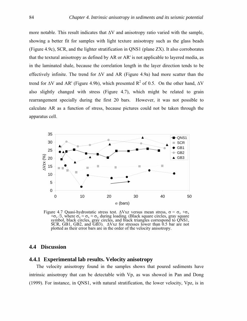
84 Chapter 4. Intrinsic anisotropy in sediments and its seismic potential
more notable. This result indicates that ∆V and anisotropy ratio varied with the sample,
showing a better fit for samples with light texture anisotropy such as the glass beads
(Figure 4.9c), SCR, and the lighter stratification in QNS1 (plane ZX). It also corroborates
that the textural anisotropy as defined by AR or AR' is not applicable to layered media, as
in the laminated shale, because the correlation length in the layer direction tends to be
effectively infinite. The trend for ∆V and AR (Figure 4.9a) had more scatter than the
trend for ∆V and AR' (Figure 4.9b), which presented R2 of 0.5. On the other hand, ∆V
also slightly changed with stress (Figure 4.7), which might be related to grain
rearrangement specially during the first 20 bars. However, it was not possible to
calculate AR as a function of stress, because pictures could not be taken through the
apparatus cell.
0
5
10
15
20
25
30
35
0 10 20 30 40 50
σ (bars)
∆Vzx
(%)
QNS1SCRGB1GB2GB3
Figure 4.7 Quasi-hydrostatic stress test. ∆Vxz versus mean stress, σ = σz +σx
+σy /3, where σz ≈ σx ≈ σy, during loading. (Black square circles, gray square symbol, black circles, gray circles, and black triangles correspond to QNS1, SCR, GB1, GB2, and GB3). ∆Vxz for stresses lower than 0.5 bar are not plotted as their error bars are in the order of the velocity anisotropy.
4.4 Discussion
4.4.1 Experimental lab results. Velocity anisotropy The velocity anisotropy found in the samples shows that poured sediments have
intrinsic anisotropy that can be detectable with Vp, as was showed in Pan and Dong
(1999). For instance, in QNS1, with natural stratification, the lower velocity, Vpz, is in

Chapter 4. Intrinsic anisotropy in sediments and its seismic potential 85
the direction perpendicular to the layers. This result indicates that the velocity responds
to the internal structure of the sample. In SCR, the highest velocity Vpx is in the direction
of the rotation axis, which has some remaining layers. However, this packing is more
complex to describe. Furthermore, the sample with the lowest ∆V, GB1, has the least
apparent segregation in the pictures. The sample with the highest ∆V, GB2, has the most
apparent segregation. This result also suggests that there is a relation between velocity
anisotropy and packing.
Figure 4.8 Hexagonal packing: (a) 2D image, (b) autocorrelation function of the
image, and (c) autocorrelation function as a function of lag (correlation distance in pixels) for azimuth angles between 0° to 180°.
For all the samples, ∆V is higher than the error of the velocity measurements (3%),
except for Vpz and Vpy in the SCR sample, and Vpx and Vpy in the QNS1, GB1 and
GB2 samples. For that reason, I can conclude that the samples show velocity anisotropy.
4.4.2 Textural anisotropy interpretation From the angles presented in Table 4.1, QNS1 has a textural anisotropy with a higher
correlation in the XY plane (0° and 180° in ZX and ZY) and a lower correlation in the Z
direction. This result agrees with the velocity anisotropy in this sample, which is Vpz <
hexagonal pack
Autocorrelation
50 100 150 200 250
50
100
150
200
250
0 20 40 60 80 100-1
-0.5
0
0.5
1
lag
AC
F
Autocorrelation vs. lag
anisotropy ratio = 5.8
correlation length = 64
theta max.= 0 180
theta min.= 50 130 Y Z

86 Chapter 4. Intrinsic anisotropy in sediments and its seismic potential
Vpx ≈Vpy. In the plane XY, AR is relatively lower than the other planes. SCR shows a
more complex textural anisotropy: there is no a clear direction of maximum and
minimum correlation in the ZX and ZY planes, while the maximum correlation is in the
X direction. This last result coincides with Vpx > Vpy ≈ Vpz for this sample.
0
20
40
0 2 4 6 8 10AR
∆V
(%)
ZYZXXY
(a)
y = 8.8xR2 = 0.5
0
20
40
0 2 4 6 8 10AR'
∆V
(%)
ZYZXXY
(b)
y = 10.4xR2 = 0.6
0
20
40
0 2 4 6 8 10AR'
∆V
(%)
ZYZXXY
(c)
Figure 4.9 Quasi-hydrostatic stress test and sample images. Velocity anisotropy,
∆V, at mean stress of 2 bars compared with (a) anisotropy ratio calculated from maximum and minimum correlation length, AR, (b) perpendicular anisotropy ratio calculated from correlation length at 0° and 90°, AR', for all samples, and (c) AR' for glass beads samples. Straight lines indicate general trends.
QNS1
QNS1

Chapter 4. Intrinsic anisotropy in sediments and its seismic potential 87
GB1 has a textural anisotropy with a maximum correlation perpendicular to the Z
direction and a minimum correlation around 30° from Z; on the XY plane there is not a
clear orientation. GB2 shows similar textural anisotropy to GB1 on the ZX and ZY
planes, but with higher AR. This result is consistent with GB2 having more segregation
than GB1. On the XY plane, the maximum correlation is in the X direction but with
lower AR than the other planes, which can imply a lower relative anisotropy in XY. GB3
has a maximum correlation perpendicular to the Z direction, and the minimum slightly
varies in ZX and ZY around the Z direction. On the XY plane, the maximum and the
minimum correlation are close to the Y direction, implying there is no clear textural
anisotropy. In general, these results mostly agree with the velocity anisotropy seen in the
glass bead samples. That is, the maximum correlation is perpendicular to the Z direction,
corresponding to a Vpz lower than Vpx and Vpy.
Therefore, AR values and the corresponding angles of anisotropy give a more
quantitative description of the sample texture. However, it seems that using the
correlation lengths at 0° and 90° to calculated AR' gives a better comparison between the
velocity anisotropy measured in perpendicular directions and the texture (perpendicular
anisotropy ratio) as is shown in Figure 4.9.
4.5 Conclusions All the results indicate that velocity anisotropy and packing are related. The
anisotropy ratio calculated from spatial autocorrelation of images gives an estimation of
packing structure. The results also suggest that if there is a relation between ∆V and
anisotropy ratio for similar isotropic stress conditions, it might work for light anisotropy
such as segregation or light stratification. Textural anisotropy as defined by AR or AR' is
not applicable to layered media because the correlation length in the layer direction tends
to be effectively infinite.
4.6 References Baxter, J., Tuzun, U., Heyes, D., Hayati, I., and Fredlund P., 1998, Stratification in
poured granular heaps: Nature, 391, 136.
Chen, Y.-C., Ishibashi, I., and Jenkins, J. T., 1998, Dynamic shear modulus and fabric:
part I, depositional and induced anisotropy: Geotechnique, 38, 25-32.
88 Chapter 4. Intrinsic anisotropy in sediments and its seismic potential
Cizeau, P., Makse, H. A., and Stanley, E., 1999, Mechanisms of granular spontaneous
stratification and segregation in two-dimensional silos: Physical Review E, 59, 4408-
4421.
Fioravante, V., and Capoferri, R., 2001, On the use of multi-directional piezoelectric
transducers in triaxial testing: Geotechnical Testing Journal, 24, 243-255.
Jiang, G-L., Tatsuoka, F., Flora, A., and Koseki, J., 1997, Inherent and stress-state-
induced anisotropy in very small strain stiffness of a sand gravel: Geotechnique, 47,
509-521.
Makse, H. A., Havlin, S., King, P., and Stanley, H. E., 1997, Spontaneous stratification in
granular mixtures: Nature, 386, 379-381.
Nur, A. and Simmons, G., 1969, Stress-induced velocity anisotropy in rock: an
experimental study: Journal of Geophysical Research, 74, 6667-6674.
Pan, Y. –W., and Dong J. –J., 1999, A micromechanics-based methodology for
evaluation the fabric of granular material: Geotechnique, 49, 761-775.
Tai, Q., and Sadd, M. H., 1997, A discrete element study of relationship of fabric to wave
propagational behaviors in granular materials: International Journal for Numerical
and Analytical Methods in Geomechanics:, 21, 295-311.
Yin, H., 1993, Acoustic velocity and attenuation of rocks; isotropy, intrinsic anisotropy,
and stress-induced anisotropy: Ph.D. Thesis, Stanford University, Stanford, CA.

89
Chapter 5 Stress-induced velocity anisotropy in sands 5.1 Introduction
It has been shown that velocity anisotropy in rocks and soft sediments can indicate
stress anisotropy (Nur and Simmons, 1969; Mavko et al., 1995; Santamarina and
Cascante, 1996; Zeng, 1999; Fioravante and Capoferri, 2001). Velocity anisotropy can be
more sensitive to stress in soft sediments than in consolidated rocks (Yin, 1993).
However, most of the studies on stress-induced velocity anisotropy have been conducted
for a wide range of compressive stresses in consolidated rocks. In soft sediments, stress-
induced velocity anisotropy has been studied only at low compressive stresses up to 8
bars (Santamarina and Cascante, 1996; Zeng, 1999; Fioravante and Capoferri, 2001).
These low compressive stresses in soft sediments represent the conditions within the first
few meters of the surface, but do not reach equally interesting deeper geophysical targets,
which can extend to hundreds or thousands of meters depth.
Stress-induced velocity anisotropy in soft sediments may be predicted with some
success using the theoretical non-linear elastic responses of acoustic waves in granular
materials (Norris and Johnson, 1997; Johnson et al., 1998; Makse et al., 1999; Sinha and
Plona, 2001). Although many models exist that attempt to predict elastic properties of
granular materials (for example, Mindlin, 1949; Dvorkin and Nur, 1996), very few
describe the effect of anisotropic stresses on velocity. The Norris and Johnson model
(Norris and Johnson, 1997; Johnson et al., 1998) is one of the few that predicts velocity
response with stress in different directions for sphere packs. This model was compared
with experimental data of a random sphere pack under uniaxial strain and reproduced,
with some limitations, the behavior of Vp versus compressive stress (Johnson et al.,
1998). Makse et al. (1999) found a linear relationship between moduli and pressure, as
opposed to the one-third-power dependency (σ1/3) predicted by the effective medium

90 Chapter 5. Stress-induced velocity anisotropy in sands
theory (Walton, 1986; Norris and Johnson, 1997) for hydrostatic stress. This linear
relationship is due to the variation of coordination number with pressure. It seems that
the Norris and Johnson model, modified by Makse’s relation between coordination
number and hydrostatic pressure dependency (I called it Makse’s correction), can be a
good first theoretical approximation for stress-induced velocity anisotropy in sands.
In Chapter 3 and 4, we studied that velocity anisotropy is related with intrinsic
anisotropy. An arisen question is also if velocity anisotropy is more affected by stress
anisotropy or intrinsic anisotropy. This chapter presents an experimental study of stress-
induced P-velocity anisotropy in unconsolidated sands at compressive measured stresses
up to 40 bars. I focus on P-wave behavior, because most of the in-situ experiments are
performed for P-waves. However, I also present some measurements of S-waves, and
compare dynamic and static elastic properties. I show measurements of stress-induced
velocity anisotropy in uniaxial strain tests with three different grain sizes and packings. I
observe that velocity anisotropy is more significantly affected by stress anisotropy than
by textural anisotropy. I find a linear dependence of velocity anisotropy on stress
anisotropy. I show that P-wave frequencies can also be related to stress anisotropy. I
encounter non-elastic strain for compressive stresses between 2 and 40 bars. In addition, I
compare the predictions of the Norris and Johnson model, Makse’s correction, and the
present experimental data, and discuss the merits and limitations of the application of
these models.
The organization of this chapter is as follows: (1) I describe the experimental test to
measure stress-induced velocity anisotropy in sands; (2) I discuss my results; (3) I
describe the Norris and Johnson model and Makse’s correction, and compare them to the
experimental results; and (4) I compare static and dynamic elastic constants.
5.2 Experimental procedure: uniaxial strain test The uniaxial strain test consists of having displacement in one direction while the
displacement in the other two perpendicular directions is constrained to zero. In this test,
the displacement is in the direction of applied compressive stress, producing induced
compressive stresses in the perpendicular directions. This stress behavior can simulate
the conditions of compaction underground in the approximation of no lateral

Chapter 5. Stress-induced velocity anisotropy in sands 91
displacement (Jaeger and Cook, 1979), where the applied compressive stress corresponds
to the overburden.
For this test, I used the polyaxial apparatus (Figure 2.5 and 2.8) and the sands (Table
2.1) described in Chapter 2. These sands were: (1) a beach sand, Santa Cruz sand (SCS),
with an average grain size of 0.25 mm, (2) another beach sand, Moss Landing sand
(MLS), with an average grain size of 0.39 mm, and (3) a construction sand, kiln dried
Monterrey sand (MS), with an average grain size of 0.91 mm. The samples were made by
raining the sand grains into the center of the polyaxial apparatus cell (see Chapter 2 for
more detailed discussion of sample preparation). I measured compressional velocity,
compressive stress, and strain in these samples in three perpendicular directions (X, Y,
and Z) under uniaxial strain. A compressive stress (σz or σzz) was applied in the vertical
(Z) direction while the loading platens in the X and Y directions remained in fixed
positions. All samples were measured during loading and unloading: SCS and MS were
measured for one cycle, and MLS for three cycles. For MLS, I also measured shear
velocity in two polarization modes for each propagation direction.
5.3 Results
5.3.1 Grain size effect and porosity Vp in our samples appears to be influenced by both grain size and porosity. Figure
5.1 shows Vp in the Z direction (Vpz). Velocities in MS (with coarser grains) were
slightly higher than velocities in SCS and MLS. The higher velocity in MS relative to
SCS can be due to MS having lower porosity. MS also had larger grain size that might
affect the velocities as it has been observed that sands with coarser grains seem to have
higher Vp than sands with finer grains (Prasad and Meissner, 1992). However, for MS
and SCS we cannot corroborate the direct effect of grain size on velocity. On the
contrary, the higher velocity in MS relative to MLS appears to be due only to MS having
larger grains, since these two samples had similar porosity (Table 2.1). In addition, MLS
(with lower porosity and larger grains than SCS) had slightly lower velocity than SCS for
compressive stresses lower than 30 bars. This finding suggests that other factors, such as
packing, may also be affecting the velocity.
Figure 5.2 shows how Vp changes with the normal stresses in each of the propagation
directions: Vpi versus σi, for i = X, Y, and Z. In all cases, the variation of Vpz with σz

92 Chapter 5. Stress-induced velocity anisotropy in sands
was smaller than the variations of Vpx and Vpy with the induced stresses, σx (σxx) and σy
(σyy), respectively. For SCS, the variation of Vpz with σz was only slightly smaller than
the variations of Vpx and Vpy with σx and σy, respectively. For MS and MLS, Vpz
showed a much smaller variation with σz than Vpx and Vpy, with σx and σy, respectively.
In addition, Vpx (roughly the same as Vpy) in MS and MLS was higher than Vpx in SCS
(Figure 5.2e); while Vpz in MS was higher than Vpz in MLS and SCS. Furthermore, it
seems that, relative to MS, MLS showed a stronger grain-size effect in the Z direction
than in the X and Y directions. On the other hand, SCS showed a strong grain-size effect
relative to MS in all directions, as a possible consequence of its finest grain size and
unstable layered packing (this packing is discussed in more detail in Chapter 4).
Instability in the packing is referred as a configuration where any singular rolling grain
causes grain flow in the rest of the sandpile (Cizeau et al., 1999).
Figure 5.2d shows the theoretical behavior of Vp and stress for all samples under an
uniaxial strain test. The model used is discussed in detail in section 5.4. This model
predicts higher Vp for larger grain size that is slighter than the one observed in Figure 5.1
and Figure 5.2e. It also predicts slower Vpz variation with σz than Vpx (Vpx=Vpy), with
σx (σx =σy), more similar to the MLS data in Figure 5.2c.
Figure 5.1 Uniaxial strain test. Vp versus applied compressive stress, σz, during loading (SCS, φ = 0.45, MS, φ = 0.41, and MLS, φ = 0.42, are indicated with purple, violet, and blue, respectively).
200
400
600
800
1000
0 10 20 30 40σz (bars)
Vpz
(m/s
)
SCSMSMLS

Chapter 5. Stress-induced velocity anisotropy in sands 93
The relation of porosity with Vp is shown in Figure 5.3 for all sands. The porosity
decreased while Vp increased during loading, and vice versa during unloading, though
final porosities were lower than initial porosities because of compaction. This same
behavior was seen for SCS, MS, and third cycle of MLS. In the two first cycles of MLS
during loading, the porosity decreased by abrupt steps while Vp increased; during
unloading the porosity gradually increased, as in the other samples. The step-like porosity
change may also be due to the packing in MLS: somehow the grains deformed elastically
during loading until reaching a point where the packing and porosity changed abruptly.
This different behavior might be affected by the different bimodal grain size distribution
in this sand (Chapter 2). In addition, the velocity change with porosity seems to be larger
in the finer-grained samples (SCS and MLS) than in the coarser-grained sample (MS).
For all sands, the strain at compressive stresses larger than 2 bars showed hysteresis
which corresponds to non-elastic behavior, in contrast to the elastic behavior found in
sands and gravels at compressive stresses lower than 1.5 bars (e.g. Jiang et al., 1997).
Figure 5.4a shows that despite the higher porosity in the SCS, its strain was lower than in
MS and MLS. It seems that SCS mostly deformed during the first stress step (Figure
5.4b). On the other hand, MS deformed more gradually with applied compressive stress
(Figure 5.4c). MLS changed shape by steps during loading: the first step (with small
deformation) at the initial compressive stress; a second step at 5.7 bars, and a final step at
22 bars (Figure 5.4d). It is possible that the grain packing in the SCS was more efficient
because of its natural stratification (and unstable packing), poorer sorting, and finer grain
sizes. Finer grains might fill the space between coarser grains and limit their movement,
and the unstable layers might be broken, having a major deformation and grain
rearrangement, at the first loading. This effect of packing or texture in the samples was
discussed in more detail in Chapter 4.

94 Chapter 5. Stress-induced velocity anisotropy in sands
(a) (b)
(c) (d)
(e) Figure 5.2 Uniaxial strain test. Vp versus compressive stresses in each direction
of propagation: Vpx, Vpy, and Vpz as functions of σx, σy, and σz, respectively in (a) SCS, (b) MS, and (c) MLS, (d) all samples (theoretical values predicted with Norris and Johnson model). (e) Vpx as a function of σx for all samples.
100
300
500
700
900
0 10 20 30 40 50σx,z (bars)
Vpx
(m/s
)SCSMSMLS
100
300
500
700
900
0 10 20 30 40 50σx,y,z (bars)
Vp (m
/s)
VpzVpxVpy
100
300
500
700
900
0 10 20 30 40 50σx,y,z (bars)
Vp (m
/s)
VpzVpxVpy
100
300
500
700
900
0 10 20 30 40 50σx,y,z (bars)
Vp
(m/s
)
VpzVpxVpy
100
300
500
700
900
0 10 20 30 40 50σx (bars)
Vpx
(m/s
)
SCSMSMLS

Chapter 5. Stress-induced velocity anisotropy in sands 95
(a)
(b)
(c)
Figure 5.3 Uniaxial strain test. Vp versus porosity, φ, for (a) SCS, (b) MS, and (c) MLS. (Initial porosity is not shown as there are not Vp measurements at that point).
0
200
400
600
800
1000
0.425 0.430 0.435 0.440 0.445φ
Vp (m
/s)
VpzVpxVpy
Cycle 1
0
200
400
600
800
1000
0.390 0.395 0.400 0.405 0.410φ
Vp (m
/s)
VpzVpxVpy
Cycle 1Cycle 3 Cycle 2
0
200
400
600
800
1000
0.390 0.395 0.400 0.405 0.410φ
Vp (m
/s)
VpzVpxVpy
Cycle 1

96 Chapter 5. Stress-induced velocity anisotropy in sands
(a)
(b) (c)
(d) Figure 5.4 Uniaxial strain test. Strain in the Z direction, εz, versus applied
compressive stress, σz. (a) Total strain minus initial strain for all samples. Total strain for (b) SCS, (b) MS, and (d) MLS.
5.3.2 Induced compressive stress As the applied compressive stress increased in the Z direction, it induced compressive
stresses in the orthogonal (X-Y) directions. Figure 5.5 shows that the induced
0.000
0.020
0.040
0.060
0 10 20 30 40 50σz (bars)
ε z
0.000
0.020
0.040
0.060
0 10 20 30 40 50σz (bars)
ε z
0.000
0.020
0.040
0.060
0 10 20 30 40 50σz (bars)
ε z
0.000
0.005
0.010
0.015
0.020
0 10 20 30 40σz (bars)
ε zSCSMSMLS

Chapter 5. Stress-induced velocity anisotropy in sands 97
compressive stresses, σx and σy, were lower during loading (normal consolidation) than
in unloading (overconsolidation), which coincides with previous results on stress
behavior in soils, even at compressive stresses lower than 8 bars (Zeng et. al., 1999;
Sivakumar et al., 2001). The stress hysteresis also corresponds to the strain hysteresis
shown in Figure 5.4. Both Figure 5.4 and Figure 5.5 display higher strain and stress
hysteresis in MLS than in SCS and MS. Nevertheless, for all samples, grain
rearrangements and a tighter packing led to an induced compressive stress accumulation
in the X and Y directions that remained during overconsolidation.

98 Chapter 5. Stress-induced velocity anisotropy in sands
(a)
(b)
(c) Figure 5.5 Uniaxial strain test. Induced compressive stresses, σx and σy, versus
applied compressive stress, σz for (a) SCS, (b) MS, and (c) MLS. (The X and Y directions are indicated with circles and squares respectively; filled symbols denote loading path, and open symbols the unloading path).
0
2
4
6
8
0 10 20 30 40σz (bars)
σ x,y (b
ars)
X
Y
0
2
4
6
8
0 10 20 30 40σz (bars)
σx,
y (ba
rs) X
Y
0
2
4
6
8
0 10 20 30 40σz (bars)
σ x,y (b
ars) Y
X

Chapter 5. Stress-induced velocity anisotropy in sands 99
(a) (b)
(c) (d)
(e) Figure 5.6 Uniaxial strain test. Ko versus applied compressive stress, σz, for (a)
SCS, (b) MS, (c) MLS first cycle, (d) MLS second cycle, and (e) MLS third cycle. Solid lines are fits for loading using equation 5.1, and dashed lines are fits for unloading using equation 5.2 (Filled circles denote loading path, and open circles the unloading path).
This stress behavior can also be studied using the ratio of horizontal to vertical
stresses, Ko = σx,y/ σz, as a function of the applied compressive stress (Figure 5.6). In all
samples, Ko showed similar dependence on σz as reported by Zeng (1999). For that
reason, it was useful to apply the empirical equations used in Zeng (1999), fitting the
parameters to the present data. These equations are as follows
0.0
0.4
0.8
1.2
0 10 20 30 40σz
Ko
0.0
0.4
0.8
1.2
0 10 20 30 40σz
Ko
0.0
0.4
0.8
1.2
0 10 20 30 40σz
Ko
0.0
0.4
0.8
1.2
0 10 20 30 40σz
Ko
0.0
0.4
0.8
1.2
0 10 20 30 40σz
Ko

100 Chapter 5. Stress-induced velocity anisotropy in sands
)sina(1Ko φ−= for loading, (5.1)
2a'sin
)OCRsina(1Koφ
φ−= for unloading, (5.2)
where a, a′ are soil constants adjustable to the data; φ is the coefficient of friction angle in
degrees (tan(φ)=0.6=µ); and OCR is the overconsolidation ratio, OCR = Kou/Kol, where
Kou is Ko during unloading, and Kol is Ko during loading (Mayne et al., 1982) calculated
from the data.
5.3.3 Vp and stress anisotropy Figure 5.7 shows the velocities in the X, Y, and Z directions as functions of applied
compressive stress for (a) SCS, (b) MS, and (c) MLS. There was a significant velocity
anisotropy in these sands, with behavior at low compressive stresses that was similar to
previously reported results (e.g. Fioravante and Capoferri, 2001). The highest velocity,
Vpz, was in the direction of applied compressive stress. The other two perpendicular
velocities, Vpx and Vpy, were roughly the same, but smaller than Vpz. As pointed out in
Chapter 2 and Chapter 4, SCS had a clear stratification. Therefore, in an isotropic stress
field, we might expect the horizontal velocities to be larger than the vertical. These
results indicate that stress anisotropy has a more significant effect on the velocity than
textural anisotropy. In addition, velocities were higher during unloading than during
loading. This velocity hysteresis was more notable in MLS, and in the directions of the
induced compressive stresses (X and Y) than in the applied compressive stress direction
(Z). This agrees with the stress hysteresis pattern found in Figure 5.5.
The sands show a faster Vp increase for stresses lower than 15 bars, and a slower Vp
increase for stresses higher than 15 bars. The steeper side of the curve has been observed
for stresses lower than 8 bars (Fioravante and Capoferri, 2001), while the behavior at
higher stresses has been seldom studied in soft sands (Yin, 1993).
I defined relative stress anisotropy (∆σ) and relative compressional velocity
anisotropy (∆Vp) as follows
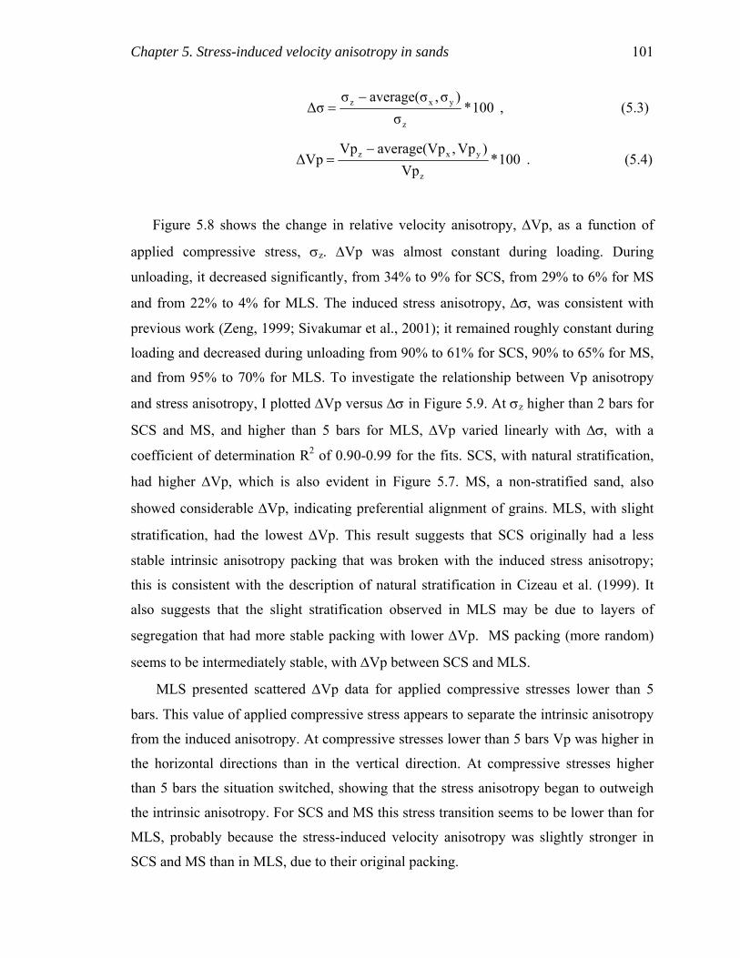
Chapter 5. Stress-induced velocity anisotropy in sands 101
100*σ
)σ,average(σσ∆σ
z
yxz −= , (5.3)
100*Vp
)Vp,average(VpVp∆Vp
z
yxz −= . (5.4)
Figure 5.8 shows the change in relative velocity anisotropy, ∆Vp, as a function of
applied compressive stress, σz. ∆Vp was almost constant during loading. During
unloading, it decreased significantly, from 34% to 9% for SCS, from 29% to 6% for MS
and from 22% to 4% for MLS. The induced stress anisotropy, ∆σ, was consistent with
previous work (Zeng, 1999; Sivakumar et al., 2001); it remained roughly constant during
loading and decreased during unloading from 90% to 61% for SCS, 90% to 65% for MS,
and from 95% to 70% for MLS. To investigate the relationship between Vp anisotropy
and stress anisotropy, I plotted ∆Vp versus ∆σ in Figure 5.9. At σz higher than 2 bars for
SCS and MS, and higher than 5 bars for MLS, ∆Vp varied linearly with ∆σ, with a
coefficient of determination R2 of 0.90-0.99 for the fits. SCS, with natural stratification,
had higher ∆Vp, which is also evident in Figure 5.7. MS, a non-stratified sand, also
showed considerable ∆Vp, indicating preferential alignment of grains. MLS, with slight
stratification, had the lowest ∆Vp. This result suggests that SCS originally had a less
stable intrinsic anisotropy packing that was broken with the induced stress anisotropy;
this is consistent with the description of natural stratification in Cizeau et al. (1999). It
also suggests that the slight stratification observed in MLS may be due to layers of
segregation that had more stable packing with lower ∆Vp. MS packing (more random)
seems to be intermediately stable, with ∆Vp between SCS and MLS.
MLS presented scattered ∆Vp data for applied compressive stresses lower than 5
bars. This value of applied compressive stress appears to separate the intrinsic anisotropy
from the induced anisotropy. At compressive stresses lower than 5 bars Vp was higher in
the horizontal directions than in the vertical direction. At compressive stresses higher
than 5 bars the situation switched, showing that the stress anisotropy began to outweigh
the intrinsic anisotropy. For SCS and MS this stress transition seems to be lower than for
MLS, probably because the stress-induced velocity anisotropy was slightly stronger in
SCS and MS than in MLS, due to their original packing.

102 Chapter 5. Stress-induced velocity anisotropy in sands
These results suggest that there is a value of applied compressive stress that
represents a transition between intrinsic anisotropy and induced stress anisotropy; the
transition stress depends on the sample. The results also confirm that near this value the
change in velocity anisotropy is a consequence of stress anisotropy variation. During
loading, the induced compressive stress in the X and Y directions increased in proportion
to the applied compressive stress, and the stress anisotropy remained constant.
Consequently, velocity anisotropy also remained constant. During unloading, the induced
compressive stresses in the XY plane did not relax in proportion to the decreasing applied
compressive stress, resulting in a decrease in stress anisotropy. This stress accumulation
(residual stress) in the XY plane during overconsolidation led to higher velocities in that
plane and lower velocity anisotropy.
The stress results could be affected by the stress inside the polyaxial cell as we saw in
Chapter 3. Hence, the stress anisotropy could be affected as well. For instance, I
estimated the stress distribution in the cell in Chapter 2, using the elastic solution of a
doubly periodic normal stress applied to the surface of a half space. For the uniaxial
strain test, I found that the measured stress in the vertical platen (σPz) was different from
the internal sample stress (σz-avg). The relation between the measured stress ratio
( PzPx / σσ ) and the internal sample stress ratio ( avgzavgx / −− σσ ) was Pz
Px
avgz
avgx
2.0 σσ
≈σσ
−
− and
Pz
Px
avgz
avgx
3.0 σσ
≈σσ
−
− for an elastic soft solid and an elastic more like a liquid, respectively.
Then, re-scaling the measured stresses with the estimated correction of Pzavgz 0.2σσ ≈−
for an elastic soft solid, I obtained that the estimated stress anisotropy inside the sample
was reduced, with positive and negative values between -97% to 74% (Figure 5.9c). The
negative values only occurred during unloading. This is consistent with the observation
shown in Figure 5.5. During frictional resistance inside the sample resulted in a reduced
stress, so that horizontal stress relaxed more slowly than the applied vertical stress. The
linear fit of ∆V to ∆σ in Figure 5.9c was still good, even with this hysteresis
phenomenon. The positive values of this stress anisotropy (8-74%) were close to the
range of the expected values in a plastic material with a friction coefficient of 0.6 (for
soft rocks). That is,

Chapter 5. Stress-induced velocity anisotropy in sands 103
z1
1
zzx 32.0))6.0(sin(tan1))6.0(sin(tan1
sin1sin1
σ=+
−σ=
θ+θ−
σ=σ−
−
, (5.5)
where tanθ is the friction coefficient. This means that assuming a soft plastic material, the
corresponding range of stress anisotropy is 0-68%. On the other hand, using the
measured stresses, the stress anisotropy range was 61-95%. Nevertheless, the estimation
of the internal stress in the samples does not give a definitive solution of this problem as
it is yet not clear what model describes better the real stress behavior in the sand in the
polyaxial apparatus. With these solutions, I only intend to give an approximate stress
range inside the samples related with the “measured stress”.

104 Chapter 5. Stress-induced velocity anisotropy in sands
(a)
(b)
(c) Figure 5.7 Uniaxial strain test. Vp versus applied compressive stress, σz, for (a)
SCS, (b) MS, and (c) MLS, first cycle. (Filled circles and continuous lines denote the loading path, and open circles and dashed lines denote the unloading path). The shown ∆Vp corresponds to the maximum applied stress velocity anisotropy.
∆Vp=34%
∆Vp=29%
∆Vp=22%
100
300
500
700
900
0 10 20 30 40σz (bars)
Vp
(m/s
)
Vpz Vpx Vpy
100
300
500
700
900
0 10 20 30 40σz (bars)
Vp
(m/s
)
Vpz Vpx Vpy
100
300
500
700
900
0 10 20 30 40σz (bars)
Vp
(m/s
)
Vpz Vpx Vpy

Chapter 5. Stress-induced velocity anisotropy in sands 105
Figure 5.8 Uniaxial strain test. Velocity anisotropy, ∆Vp, versus applied
compressive stress, σz. (Filled circles and continuous lines denote the loading path, and open circles and dashed lines denote the unloading path).
0
10
20
30
40
0 10 20 30 40σz (bars)
∆Vp
(%)
SCSMSMLS
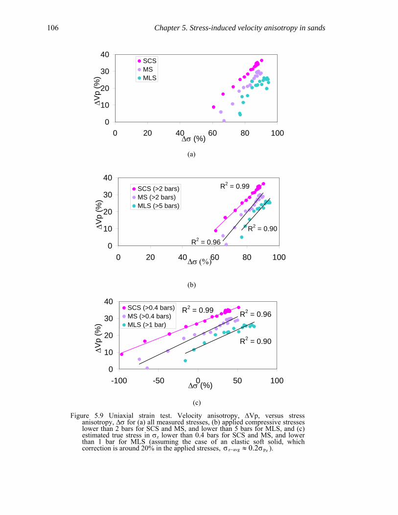
106 Chapter 5. Stress-induced velocity anisotropy in sands
(a)
(b)
(c) Figure 5.9 Uniaxial strain test. Velocity anisotropy, ∆Vp, versus stress
anisotropy, ∆σ for (a) all measured stresses, (b) applied compressive stresses lower than 2 bars for SCS and MS, and lower than 5 bars for MLS, and (c) estimated true stress in σz lower than 0.4 bars for SCS and MS, and lower than 1 bar for MLS (assuming the case of an elastic soft solid, which correction is around 20% in the applied stresses, Pzavgz 0.2σσ ≈− ).
R2 = 0.99 R2 = 0.96
R2 = 0.90
0
10
20
30
40
-100 -50 0 50 100∆σ (%)
∆V
p (%
)
SCS (>0.4 bars)MS (>0.4 bars)MLS (>1 bar)
R2 = 0.99
R2 = 0.96
R2 = 0.90
0
10
20
30
40
0 20 40 60 80 100∆σ (%)
∆V
p (%
)
SCS (>2 bars)MS (>2 bars)MLS (>5 bars)
0
10
20
30
40
0 20 40 60 80 100∆σ (%)
∆Vp
(%)
SCSMSMLS

Chapter 5. Stress-induced velocity anisotropy in sands 107
5.3.4 Comparison with other data I compared the results of SCS (finest-grain) and MS (coarsest-grain) with other
acoustic data from sands to find the differences and similarities with previous studies on
sands. For this task I used three sets of data: one is referred to as Yin’s data (Yin, 1993),
other as Prasad’s data (Prasad and Meissner, 1992), and the last one as Zimmer (Zimmer,
2003). Results of triaxial stress tests in Ottawa sand made by Yin (Yin’s data) are shown
in Figure 5.10. Yin (1993) applied compressive stress in the three Cartesian directions by
varying σz and maintaining σx and σy at 17.2 bars. Results of hydrostatic stress
experiments for fine and coarse sands made by Prasad and Meissner (Prasad’s data) are
also shown in Figure 5.10a and Figure 5.10b, respectively. In addition, velocities
measured in SCS under hydrostatic pressure at frequency of 20KHz made by Zimmer
(2003) are shown in Figure 5.10.
In Figure 5.10a, data for SCS is compared with Prasad’s data for a fine sand, Yin’s
data for Ottawa sand, and SCS measured at frequency of 20KHz. We notice that in SCS
measured under uniaxial strain test, Vpz and Vpy were lower than Yin’s Vpz and Vpy,
Prasad’s Vp for fine grained sand, same SCS measured under hydrostatic pressure. This
difference in velocity is most likely because Yin’s, Prasad’s, and Zimmer’s experiments
were not at uniaxial strain, as was observed in Chapter 3. In our uniaxial strain
experiments, the samples were compressed only in the Z direction, inducing compressive
stresses lower than 17.5 bars in the X and Y directions (Figure 5.5). Hence, the samples
were effectively less compressed. In Figure 5.10b, MS is compared with Prasad’s data for
a coarse sand and Yin’s data for Ottawa sand. As for SCS (Figure 5.10a), Vpz and Vpy in
MS were lower than Yin’s and Prasad’s data. These results also corroborate the findings
in Chapter 3, where velocities under hydrostatic stress were found to be higher than
velocities under isotropic compressive stress in the polyaxial apparatus.

108 Chapter 5. Stress-induced velocity anisotropy in sands
(a)
(b)
Figure 5.10 Comparison of Vp for different sands and tests. Velocity as a
function of applied compressive stress for (a) fine grained sands comparison under uniaxial strain test (SCS), uniaxial stress test (Yin), and hydrostatic pressure (Prasad, and Zimmer); and (b) coarse grained sands comparison under uniaxial strain test (MS), uniaxial stress test (Yin), and hydrostatic pressure (Prasad).
5.3.5 Vp and frequency To find the dominant frequency in the waveforms, I used the program “Spectrum
Division”, which calculates the Fourier transform of the waves to obtain signals in the
frequency domain. The frequency at the maximum amplitude of these signals was taken
as the dominant frequency of the waves.
200
300
400
500
600
700
800
900
0 10 20 30 40σz (bars)
Vp
(m/s
)
SCS Yin Prasad Zimmer
Vpz
Vpy
VpzVpy
VpVp
200
300
400
500
600
700
800
900
0 10 20 30 40σz (bars)
Vp
(m/s
)
MS Yin Prasad
Vpz
Vpy
VpzVpy
Vp
Chapter 5. Stress-induced velocity anisotropy in sands 109
Figure 5.11 shows that the P-waveforms in X, Y, and Z had different dominant
frequencies, which are lower than the source frequency (1MHz) due to attenuation. In
SCS and MS, the frequency of the P-wave propagating in Z increased with compressive
stress during loading, and decreased with compressive stress during unloading. The
frequency of the P-wave propagating in Z was higher than that of the P-wave propagating
in X and Y. The signal frequency was also higher for SCS than for MS. For MS, the
frequencies of the signals in X and Y increased with stress for compressive stresses lower
than 14 bars and then remained fairly constant at about 16.2 KHz. For SCS, these
frequencies were constant at 17 KHz for all compressive stresses.
On the other hand, MLS showed a different frequency-stress behavior than SCS and
MS. At compressive stresses lower than 2 bars for X and Y, and 7 bars for Z, all
frequencies increased with compressive stress during loading and decreased with
compressive stress during unloading. At higher compressive stresses, the frequencies
were constant at 15, 12.5, and 17 KHz for X, Y, and Z, respectively.
These results may indicate that frequency anisotropy is related to stress-induced
velocity anisotropy. The highest frequency difference between the X, Y, and Z directions
appeared in SCS (Figure 5.11a), corresponding to the highest velocity anisotropy (Figure
5.7a and Figure 5.9). A lower frequency difference in MS (Figure 5.16b) corresponded to
lower velocity anisotropy (Figure 5.7b and Figure 5.9). Finally, the smallest frequency
difference, with no preferential direction in frequency, was found in MLS, which had the
lowest velocity anisotropy (Figure 5.7c and Figure 5.8).
In addition, the corresponding mean wavelengths (λp') were 2.5, 3.6, and 3.8 cm for
SCS, MS, and MLS, respectively. This means that the wavelengths were much larger
than the mean grain sizes, which helps to justify the use of effective medium theory.
These wavelengths were around 2 to 3 times the sample lengths, with wavelength
resolution (λp'/4) of 0.63, 0.9, and 0.95 cm for SCS, MS, and MLS, respectively. In other
words, heterogeneity sizes lower than these resolutions, such as grains and thin layers
(<λp'/4), were not detected with the P-waves, just seen as an “average”.

110 Chapter 5. Stress-induced velocity anisotropy in sands
(a)
(b)
(c) Figure 5.11 Uniaxial strain test. P-wave frequency as a function of applied
compressive stress for (a) SCS, (b) MS, and (c) MLS.
0
5
10
15
20
25
30
35
40
0 5 10 15 20 25 30 35 40 45σz (bars)
Freq
uenc
y (K
Hz)
Vpz
Vpx
Vpy
0
10
20
30
40
0 5 10 15 20 25 30 35 40 45σz (bars)
Freq
uenc
y (K
Hz)
Vpz
Vpx
Vpy
0
10
20
30
40
0 5 10 15 20 25 30 35 40 45σz (bars)
Freq
uenc
y (K
Hz)
Vpz
Vpx
Vpy

Chapter 5. Stress-induced velocity anisotropy in sands 111
5.3.6 Vs and stress anisotropy Shear waves often are difficult to acquire in soft sediments, especially at low
compressive stresses. I measured Vs at compressive stresses higher than 15-20 bars in
MLS. Figure 5.12 introduces the Vs notation used here, the arrows represent polarization
direction. Figure 5.13 shows these velocities in the Z, X and Y directions in two
polarization directions (Vs1 and Vs2). In the propagation direction Z (Figure 5.13a),
Vs1z was polarized in the direction of X (Vzx), and Vs2z was polarized in the direction
of Y (Vzy). Vs1z and Vs2z were similar, as we would expect, since both of them were
polarized in the plane of induced compressive stresses (XY). In the propagation direction
X (Figure 5.13b), Vs1x was polarized in Y (Vxy), and Vs2x was polarized in Z (Vxz).
Again as we would expect, Vs1x and Vs2x showed anisotropy, with Vs1x (polarized in
the direction of the induced compressive stress σy) lower than Vs2x (polarized in the
direction of applied compressive stress σz). Vs1y (Vyx) and Vs2y (Vyz) showed similar
behavior (Figure 5.13b). The shear velocities changed only slightly from cycle to cycle,
as did Vp, as a consequence of the very small compaction at these compressive stresses.
Figure 5.14a and Figure 5.14b show that Vzx was higher than Vxz, and Vzy was
higher than Vyz. The difference was around 15% on the ZX plane, and 30% on the ZY
plane. On the other hand, Vxy and Vyx showed similar velocities (Figure 5.14c), with an
average difference of 6%. In other words, the higher velocities were for Vs propagating
in Z where σz > σx ≈ σy. The significant Vs difference was on ZX and ZY, such as the
shear-velocities propagating in Z were higher than the shear-velocities polarizing in Z.
These results suggest that the propagation direction is more sensitive to the stress
anisotropy than the polarization direction.
Figure 5.12 Sketch of shear waves notation. Arrows show polarization directions.
Vzy=Vs2zVzx=Vs1z
Vyz=Vs2yVyx=Vs1y
Vxz=Vs2xVxy=Vs1x
Z
Y
X
Vzy=Vs2zVzx=Vs1z
Vyz=Vs2yVyx=Vs1y
Vxz=Vs2xVxy=Vs1x
Z
Y
X

112 Chapter 5. Stress-induced velocity anisotropy in sands
(a)
(b)
(c) Figure 5.13 Uniaxial strain test. Shear velocity in MLS first cycle in the direction
of propagation of (a) Z, (b) X, and (c) Y, as a function of applied compressive stress, σz.
100
200
300
400
500
600
0 10 20 30 40σz (bars)
Vs
(m/s
)
Vs1x
Vs2x
100
200
300
400
500
600
0 10 20 30 40 50σz (bars)
Vs
(m/s
)
Vs1y
Vs2y
100
200
300
400
500
600
0 10 20 30 40σz (bars)
Vs
(m/s
)
Vs1z
Vs2z

Chapter 5. Stress-induced velocity anisotropy in sands 113
(a)
(b)
(c) Figure 5.14 Uniaxial strain test. Shear velocity as a function of applied
compressive stress, σz. Comparison in the (a) ZX plane: Vs1z=Vzx and Vs2x=Vxz, (b) ZY plane: Vs2z=Vzy and Vs2y=Vyz, and (c) XY plane: Vs1x=Vxy and Vs1y=Vyx.
100
200
300
400
500
600
0 10 20 30 40σz (bars)
Vs
(m/s
)
Vs1z
Vs2x
100
200
300
400
500
600
0 10 20 30 40σz (bars)
Vs
(m/s
)
Vs2y
Vs2z
100
200
300
400
500
600
0 10 20 30 40σz (bars)
Vs
(m/s
)
Vs1x
Vs1y

114 Chapter 5. Stress-induced velocity anisotropy in sands
5.3.7 Vs and frequency Figure 5.15 shows that S waves contained higher frequency at higher compressive
stresses. These frequencies were higher (1-80 KHz) and more scattered than the P-wave
frequencies (0-17 KHz). S-waves propagating in Z had higher frequencies than S-waves
propagating in X and Y, as was true for P-waves (Figure 5.11c). However, S-wave
frequencies for waves propagating in X and Y were more scattered than the
corresponding P-wave frequencies. This result indicates that the S-wave frequencies
cannot be clearly related to stress-induced anisotropy in MLS, perhaps because MLS
showed the lowest velocity anisotropy.
In addition, the corresponding mean wavelength (λs') was 0.7cm, which was much
larger than the mean grain size. This wavelength was around 10 times smaller than the
sample length with a wavelength resolution (λs'/4) of 0.18 cm.

Chapter 5. Stress-induced velocity anisotropy in sands 115
(a)
(b) Figure 5.15 Uniaxial strain test. S-wave frequency in all directions as a function
of (a) applied compressive stress, and (b) each stress direction.
5.4 Model and experiments comparison
5.4.1 Norris and Johnson model (Nonlinear Elasticity of granular media)
Norris and Johnson (1997) developed an effective medium theory (EMT) of non-
linear elasticity. It is derived from the analysis of energy in a random sphere pack for
0
10
20
30
40
50
60
70
80
90
0 10 20 30 40 50σz (bars)
Freq
uenc
y (K
Hz)
Vs1zVs2zVs1xVs2xVs1yVs2y
0
10
20
30
40
50
60
70
80
90
0 10 20 30 40 50σx,y,z (bars)
Freq
uenc
y (K
Hz)
Vs1zVs2zVs1xVs2xVs1yVs2y
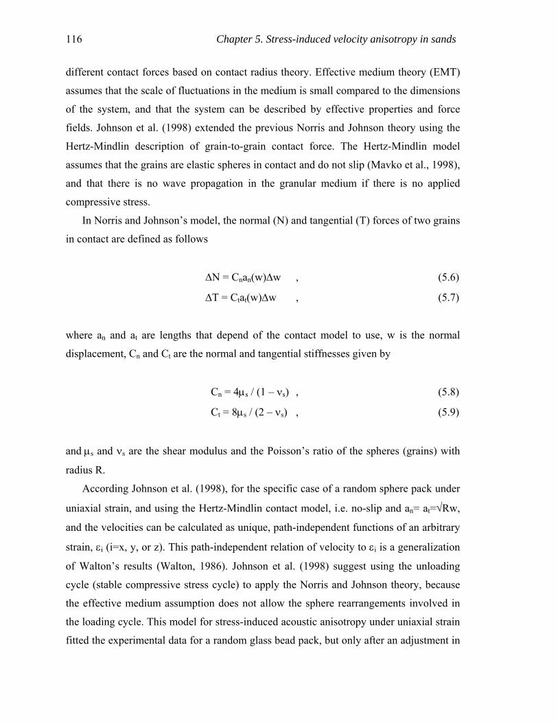
116 Chapter 5. Stress-induced velocity anisotropy in sands
different contact forces based on contact radius theory. Effective medium theory (EMT)
assumes that the scale of fluctuations in the medium is small compared to the dimensions
of the system, and that the system can be described by effective properties and force
fields. Johnson et al. (1998) extended the previous Norris and Johnson theory using the
Hertz-Mindlin description of grain-to-grain contact force. The Hertz-Mindlin model
assumes that the grains are elastic spheres in contact and do not slip (Mavko et al., 1998),
and that there is no wave propagation in the granular medium if there is no applied
compressive stress.
In Norris and Johnson’s model, the normal (N) and tangential (T) forces of two grains
in contact are defined as follows
∆N = Cnan(w)∆w , (5.6)
∆T = Ctat(w)∆w , (5.7)
where an and at are lengths that depend of the contact model to use, w is the normal
displacement, Cn and Ct are the normal and tangential stiffnesses given by
Cn = 4µs / (1 – νs) , (5.8)
Ct = 8µs / (2 – νs) , (5.9)
and µs and νs are the shear modulus and the Poisson’s ratio of the spheres (grains) with
radius R.
According Johnson et al. (1998), for the specific case of a random sphere pack under
uniaxial strain, and using the Hertz-Mindlin contact model, i.e. no-slip and an= at=√Rw,
and the velocities can be calculated as unique, path-independent functions of an arbitrary
strain, εi (i=x, y, or z). This path-independent relation of velocity to εi is a generalization
of Walton’s results (Walton, 1986). Johnson et al. (1998) suggest using the unloading
cycle (stable compressive stress cycle) to apply the Norris and Johnson theory, because
the effective medium assumption does not allow the sphere rearrangements involved in
the loading cycle. This model for stress-induced acoustic anisotropy under uniaxial strain
fitted the experimental data for a random glass bead pack, but only after an adjustment in

Chapter 5. Stress-induced velocity anisotropy in sands 117
the normal and tangential stiffness ratio (Johnson et al., 1998), which may indicate that
there is slip between the grains that “lowers” the apparent stiffness.
Makse et al. (1999) found that the coordination number (n) depends on the
hydrostatic pressure (p) as follows
n(p) = 6 + ( p / 0.06 MPa )1/3. (5.10)
In this section, I introduce this dependency into the equations of Johnson et al. (1998)
as a correction. I use σ = (σx + σy + σz)/3 as an approximation of p. I calculate Vpz,
Vpx=Vpy=Vpxy, σz, and σx=σy using the Norris and Johnson model with and without
Makse’s correction (Equation 5.10). The input parameters are: shear modulus and
Poisson ratio (using values for quartz, as these sands were predominantly quartz), density
of the grains, the permanent strain (1e-6) after stress cycles, initial porosity, grain size,
and an average coordination number (for the Norris and Johnson model without Makse’s
correction). My experimental data are the Vpz, Vpx, and Vpy (Vpxy = (Vpx+Vpy)/2) in
the unloading cycle for uniaxial strain in SCS and MS.
In the Norris and Johnson model, I find that a coordination number of 5 fits the data
best for both samples. However, this value is unrealistic, because the packing with the
lowest coordination number is simple cubic, with n=6, for 0.476 porosity (Mavko et al.,
1998; Santamarina, 2001). Using n > 5 or Makse’s correction in the model, I find that the
model overestimates velocity values. Therefore, as suggested by Johnson et al. (1998), I
adjust the model by changing the values of Cn. Thus, the grain normal effective stiffness
is reduced or increased by a factor (γ), such that Cn′= γCn.
5.4.2 Velocity and compressive stress Figure 5.16 and Figure 5.17 show measured and predicted velocities versus the
applied compressive stress (σz) for SCS and MS, respectively. The top graphics (Figure
5.16a and 5.18a) show the model predictions without adjustments in Cn, and the bottom
graphics correspond to an adjusted Cn. For both samples, Makse’s correction slightly
improved the match between the modeled and measured Vp (Vpz and Vpxy) as a
function of σz. Without the Cn adjustment, there is a good fit of Vpxy as a function of σz

118 Chapter 5. Stress-induced velocity anisotropy in sands
for both samples. Vpz as a function of σz was overestimated, and the predicted behavior
seemed to differ slightly from the lab data. Also, the model overestimated the sensitivity
of Vpxy to the induced compressive stress, σx,y, (Figure 5.18 and Figure 5.19). In other
words, the model duplicated fairly well the dependence of Vpxy on the applied
compressive stress but did not match the dependence of Vpxy on the induced
compressive stresses for the uniaxial strain test in sands.
I found that the best adjustable Cn for SCS was 150 GPa (Figure 5.16b); for MS, the
best value was 130 GPa (Figure 5.17b). These Cn values were lower than the Cn
calculated in equation 5.8 (191 GPa) and the Ct calculated in equation 5.9 (183 GPa). As
a result, γ < 1 or Cn′< Cn. γ was 0.78 for SCS, and 0.68 for MS, while it was 0.74 for the
glass beads in Johnson (1998), which may indicate that there is slip between the grains
that “lowers” the apparent stiffness. Nevertheless, these adjustments in the Norris and
Johnson model need to be investigated further.
Figure 5.20 shows predictions using the coordination number n=6 in the Norris and
Johnson model, and the coordination number calculated in Makse’s correction. It seems
that Makse’s correction does not significantly affect the model’s prediction in the range
of compressive stresses studied here. This effect can be seen in Figures 5.17 to 5.19.

Chapter 5. Stress-induced velocity anisotropy in sands 119
(a)
(b) Figure 5.16 Vp versus applied compressive stress for the Norris and Johnson
model, and experimental data comparison in SCS for. (a) Cn from equation 5.8, and (b) adjusted Cn. (Uniaxial strain test).
0 1 2 3 4 5200
300
400
500
600
700
800
900
σz (MPa)
Vp
(m/s
)
Cn = 150000MPa
Vpz( SCS)Norris&Johnson (n=6)Makse-correctionVpxy( SCS)
0 1 2 3 4 5200
300
400
500
600
700
800
900
σz (MPa)
Vp
(m/s
)
Cn = 191304MPa
Vpz( SCS)Norris&Johnson (n=6)Makse-correctionVpxy( SCS)

120 Chapter 5. Stress-induced velocity anisotropy in sands
(a)
(b)
Figure 5.17 Vp versus applied compressive stress for the Norris and Johnson
model, and experimental data comparison in MS: (a) Cn from equation 5.8, and (b) adjusted Cn. (Uniaxial strain test).
0 1 2 3 4 5200
300
400
500
600
700
800
900
σz (MPa)
Vp
(m/s
)
Cn = 191304MPa
Vpz( MS)Norris&Johnson (n=6)Makse-correctionVpxy( MS)
0 1 2 3 4 5200
300
400
500
600
700
800
900
σz (MPa)
Vp
(m/s
)
Cn = 130000MPa
Vpz( MS)Norris&Johnson (n=6)Makse-correctionVpxy( MS)

Chapter 5. Stress-induced velocity anisotropy in sands 121
(a)
(b)
Figure 5.18 Vp versus induced compressive stress for the Norris and Johnson
model, and experimental data comparison in SCS: (a) Cn from equation 5.8, and (b) adjusted Cn. (Uniaxial strain test).
0 0.2 0.4 0.6 0.8200
300
400
500
600
700
800
900
σx, σy (MPa)
Vp
(m/s
)
Cn = 191304MPa
Vpx( SCS)Vpy( SCS)Norris&Johnson (n=6)Makse-correction
0 0.2 0.4 0.6 0.8200
300
400
500
600
700
800
900
σx, σy (MPa)
Vp
(m/s
)
Cn = 150000MPa
Vpx( SCS)Vpy( SCS)Norris&Johnson (n=6)Makse-correction

122 Chapter 5. Stress-induced velocity anisotropy in sands
(a)
(b) Figure 5.19 Vp versus induced compressive stress the for Norris and Johnson
model, and experimental data comparison in MS: (a) Cn from equation 5.8, and (b) adjusted Cn. (Uniaxial strain test).
0 0.2 0.4 0.6 0.8200
300
400
500
600
700
800
900
σx, σy (MPa)
Vp
(m/s
)
Cn = 191304MPa
Vpx( MS)Vpy( MS)Norris&Johnson (n=6)Makse-correction
0 0.2 0.4 0.6 0.8200
300
400
500
600
700
800
900
σx, σy (MPa)
Vp
(m/s
)
Cn = 130000MPa
Vpx( MS)Vpy( MS)Norris&Johnson (n=6)Makse-correction

Chapter 5. Stress-induced velocity anisotropy in sands 123
Figure 5.20 Coordination number versus applied compressive stress for the
Norris and Johnson model, and experimental data comparison (SCS).
5.4.3 Static stress-strain I also compared the stress-strain curves obtained in the modeling and the
experimental data, and I found a mismatch (Figure 5.21 and Figure 5.23). Assuming that
the main difference between the modeled and experimental strain was due to the first
deformation-gap, I shifted the modeled data by the initial experimental strain (Figures
5.23 and Figure 5.24). We can see that the general stress-strain behavior was predicted
for the models, except for the initial strains and the first deformation-gap (Figure 5.21-
5.24).
10-2 10-1 100 1014
5
6
7
8
9
10
11
12
σz (MPa)
N(P
)
Cn = 191304MPa Makse-correctionNorris&Johnson (n=6)

124 Chapter 5. Stress-induced velocity anisotropy in sands
(a)
(b) Figure 5.21 Strain versus applied compressive stress for the Norris and Johnson
model, and experimental data comparison in SCS: (a) Cn from equation 5.7, and (b) adjusted Cn. (Uniaxial strain test).
0 1 2 3 4 50
0.005
0.01
0.015
0.02
ε z
σz(MPa)
Cn = 191304MPa
SCSNorris&Johnson (n=6)Makse-correction
0 1 2 3 4 50
0.005
0.01
0.015
0.02
ε z
σz(MPa)
Cn = 150000MPa
SCSNorris&Johnson (n=6)Makse-correction

Chapter 5. Stress-induced velocity anisotropy in sands 125
(a)
(b)
Figure 5.22 Strain versus applied compressive stress for the Norris and Johnson
model (shifted), and experimental data comparison in SCS: (a) Cn from equation 5.8, and (b) adjusted Cn. (Uniaxial strain test).
0 1 2 3 4 50
0.005
0.01
0.015
0.02
0.025
0.03
ε z
σz(MPa)
Cn = 191304MPa SCSNorris&Johnson (n=6)Makse-correction
0 1 2 3 4 50
0.005
0.01
0.015
0.02
0.025
0.03
ε z
σz(MPa)
Cn = 150000MPa SCSNorris&Johnson (n=6)Makse-correction

126 Chapter 5. Stress-induced velocity anisotropy in sands
(a)
(b)
Figure 5.23 Strain versus applied compressive stress for the Norris and Johnson
model, and experimental data comparison in MS: (a) Cn from equation 5.8, and (b) adjusted Cn. (Uniaxial strain test).
0 1 2 3 4 50
0.005
0.01
0.015
0.02
ε z
σz(MPa)
Cn = 191304MPa
MSNorris&Johnson (n=6)Makse-correction
0 1 2 3 4 50
0.005
0.01
0.015
0.02
ε z
σz(MPa)
Cn = 130000MPa
MSNorris&Johnson (n=6)Makse-correction

Chapter 5. Stress-induced velocity anisotropy in sands 127
(a)
(b) Figure 5.24 Strain versus applied compressive stress for the Norris and Johnson
(shifted) model, and experimental data comparison in MS: (a) Cn from equation 5.8, and (b) adjusted Cn. (Uniaxial strain test).
5.4.4 Model comparison: infinitely rough and infinitely smooth The Norris and Johnson theory with Hertz-Mindlin model (infinitely rough contact)
was shown in the previous sections. In this section, I compare this model for both
infinitely rough contacts (no slip and an=at= √Rw), and infinitely smooth contacts (at=0).
0 1 2 3 4 50
0.005
0.01
0.015
0.02
0.025
0.03
ε z
σz(MPa)
Cn = 191304MPa MSNorris&Johnson (n=6)Makse-correction
0 1 2 3 4 50
0.005
0.01
0.015
0.02
0.025
0.03
ε z
σz(MPa)
Cn = 130000MPa MSNorris&Johnson (n=6)Makse-correction

128 Chapter 5. Stress-induced velocity anisotropy in sands
Figure 5.25 shows Vp as a function of the applied compressive stress for both
samples. We can see that the model prediction for Vpz was slightly better for the
infinitely smooth contact (Figure 5.25) than for the infinitely rough contact (Figure 5.16a
and 5.17a), and this prediction was better for MS than for SCS. Vpxy was underestimated
in the infinitely smooth contact model, while in Figure 5.16a and 5.17a the model
matched the experimental data well. In addition, Vpxy as a function of the induced
compressive stress (Figure 5.26) was better-predicted by the infinitely smooth contact
than by the former model, which overestimated with Norris and Johnson, and
underestimated with Makse’s correction. Nevertheless, this model was still far from the
experimental data. In addition, there was no difference in stress-strain behavior between
the infinitely rough and infinitely smooth models.

Chapter 5. Stress-induced velocity anisotropy in sands 129
(a)
(b)
Figure 5.25 Vp versus applied compressive stress for the Norris and Johnson
model (infinitely smooth), and experimental data comparison in (a) SCS, and (b) MS. (Uniaxial strain test).
0 1 2 3 4 5200
300
400
500
600
700
800
900
σz (MPa)
Vp
(m/s
)
Cn = 191304MPa
Vpz( SCS)Norris&Johnson (n=6)Makse-correctionVpxy( SCS)
0 1 2 3 4 5200
300
400
500
600
700
800
900
σz (MPa)
Vp
(m/s
)
Cn = 191304MPa
Vpz( MS)Norris&Johnson (n=6)Makse-correctionVpxy( MS)

130 Chapter 5. Stress-induced velocity anisotropy in sands
(a)
(b) Figure 5.26 Vp versus induced compressive stress for the Norris and Johnson
model (infinitely smooth), and experimental data comparison in (a) SCS, and (b) MS. (Uniaxial strain test).
0 0.2 0.4 0.6 0.8200
300
400
500
600
700
800
900
σx, σy (MPa)
Vp
(m/s
)
Cn = 191304MPa
Vpx( SCS)Vpy( SCS)Norris&Johnson (n=6)Makse-correction
0 0.2 0.4 0.6 0.8200
300
400
500
600
700
800
900
σx, σy (MPa)
Vp
(m/s
)
Cn = 191304MPa
Vpx( MS)Vpy( MS)Norris&Johnson (n=6)Makse-correction

Chapter 5. Stress-induced velocity anisotropy in sands 131
5.5 Static and dynamic elastic constants comparison Dynamic elastic constants, derived from Vp and Vs, can be different from static
constants derived from stress-strain relations (Jaeger and Cook, 1979). For example,
Cheng and Johnston (1981) showed that the ratio between the static and dynamic bulk
moduli, Ks/Kd, at atmospheric pressure is lower for samples with higher crack porosity:
Ks/Kd is around 0.15 for tuff, 0.4-0.5 for sandstones, and 0.5 for granite.
In this section, I compare dynamic and static elastic constants for MLS, which had
both P and S waves measurements. Dynamic constants were calculated using the
following equations:
1)VsizVpz(
2)VsizVpz(
21
2
2
id
−
−=ν (5.11)
)Vsiz34Vpz(K 22
id −ρ= (5.12)
)21(K3E ididid ν−= (5.13)
2id VsizG ρ= , (5.14)
where νd, Kd, Ed, and Gd are the dynamic Poisson ratio, bulk modulus, Young’s modulus,
and shear modulus, respectively; i=1 or 2, corresponding to X or Y polarization,
respectively. The propagation of the velocities was taken in the Z direction, which was
the applied compressive stress direction.
Static constants were calculated using the following equations for uniaxial strain:
o
os K
K+
=1
ν (5.15)
z
zsM
εσ
= (5.16)
)1()21)(1(
ννν
−−+
=MEs (5.17)

132 Chapter 5. Stress-induced velocity anisotropy in sands
)1(3)1(
νν
−+
=MKs (5.18)
43 KMGs
−= (5.19)
where νs, Ms, Ks, Es, and Gs are the static Poisson ratio, P wave modulus, bulk modulus,
Young’s modulus, and shear modulus, respectively; εz and σz are is the strain and stress
in Z, respectively. All of these equations are approximate, because they assume an elastic
and isotropic material.
I found that both dynamic and static Poisson ratio depend on compressive stress: the
higher the compressive stress, the higher the Poisson ratio. Dynamic Poisson ration also
depended on the propagation and polarization directions of the shear waves: (1) for Vs
propagating in Z and polarized in both X and Y, νd ranged from 0.15 to 0.31; (2) for Vs
propagating in X and polarized in Y, νd ranged from 0.33 to 0.35; (3) for Vs propagating
in X and polarized in Z, νd ranged from 0 to 0.18; (4) for Vs propagating in Y and
polarized in X, νd ranged from 0.33 to 0.41; and (5) for Vs propagating in Y and
polarized in Z, νd ranged from 0.18 to 0.28. Static Poisson ratio, which was calculated
from the stress ratio, ranged from 0.05 to 0.33.
Figure 5.27 compares dynamic and static Poisson ration (νs/νd) as functions of
applied compressive stress for three loading cycles. In the first cycle, νs/νd in X (red
points) had values around 1 that fluctuated at compressive stresses lower than 25 bars.
On the other hand, νs/νd in Y increased with compressive stress during loading (blue
closed points), and was almost constant at 0.8 for unloading (blue open points). In the
second cycle, νs/νd for both X and Y directions was around 0.95 for compressive stresses
higher than 10 bars. In the third cycle, νs/νd was around 0.88 for all compressive stresses.
This result indicates that νs/νd tends to stabilize after the main rearrangement in the first
cycle.
Figure 5.28, 5.29, and 5.30 show the ratio of static and dynamic Young’s, bulk, and
shear moduli, respectively, as functions of applied compressive stress. All these ratios
presented similar trends: the higher the compressive stress, the higher the ratio, as we
seen in the sandstones and granites studied by Cheng and Johnston (1981). In the first

Chapter 5. Stress-induced velocity anisotropy in sands 133
cycle, for compressive stresses lower than 30 bars during loading, the ratios were higher
than for higher compressive stresses and unloading. It seems that during loading below
30 bars, rearrangement occurred; while during unloading, and also during loading above
30 bars, and during subsequent cycles there was little rearrangement and little difference
between X and Y directions.

134 Chapter 5. Stress-induced velocity anisotropy in sands
(a)
(b)
(c) Figure 5.27 Uniaxial strain test. Ratio of static and dynamic Poisson’s ratios,
νs/νd, as a function of applied compressive stress, σz, in MLS for: (a)first cycle, (b) second cycle, and (c) third cycle. ((x,s1) indicates Vs propagating in Z and polarized in S1(X), and (y,s2) indicates Vs propagating in Z and polarized in S2(Y)).
0.00
0.40
0.80
1.20
0 10 20 30 40 50σz (bars)
νs/ ν
d
(x,s1)
(y, s2)
0.00
0.40
0.80
1.20
0 10 20 30 40 50σz (bars)
νs/ ν
d
(x,s1)
(y, s2)
0.00
0.40
0.80
1.20
0 10 20 30 40 50σz (bars)
νs/ ν
d
(x,s1)
(y, s2)

Chapter 5. Stress-induced velocity anisotropy in sands 135
(a)
(b)
(c) Figure 5.28 Uniaxial strain test. Ratio of static and dynamic bulk moduli, Ks/Kd,
as a function of applied compressive stress, σz, in MLS for: (a)first cycle, (b) second cycle, and (c) third cycle. ((x,s1) indicates Vs propagating in Z and polarized in S1(X), and (y,s2) indicates Vs propagating in Z and polarized in S2(Y)).
0.00
0.02
0.04
0.06
0.08
0.10
0.12
0.14
0 10 20 30 40 50σz (bars)
Ks/
Kd
(x,s1)
(y, s2)
0.00
0.02
0.04
0.06
0.08
0.10
0.12
0.14
0 10 20 30 40 50σz (bars)
Ks/
Kd
(x,s1)
(y,s2)
0.00
0.02
0.04
0.06
0.08
0.10
0.12
0.14
0 10 20 30 40 50σz (bars)
Ks/
Kd
(x,s1)
(y,s2)

136 Chapter 5. Stress-induced velocity anisotropy in sands
(a)
(b)
(c) Figure 5.29 Uniaxial strain test. Ratio of static and dynamic Young’s moduli,
νs/νd, as a function of applied compressive stress, σz, in MLS for: (a)first cycle, (b) second cycle, and (c) third cycle. ((x,s1) indicates Vs propagating in Z and polarized in S1(X), and (y,s2) indicates Vs propagating in Z and polarized in S2(Y)).
0.00
0.05
0.10
0.15
0.20
0.25
0 10 20 30 40 50σz (bars)
Es/
Ed
(x,s1)
(y, s2)
0.00
0.05
0.10
0.15
0.20
0.25
0 10 20 30 40 50σz (bars)
Es/
Ed
(x,s1)
(y, s2)
0.00
0.05
0.10
0.15
0.20
0.25
0 10 20 30 40 50σz (bars)
Es/
Ed
(x,s1)
(y, s2)
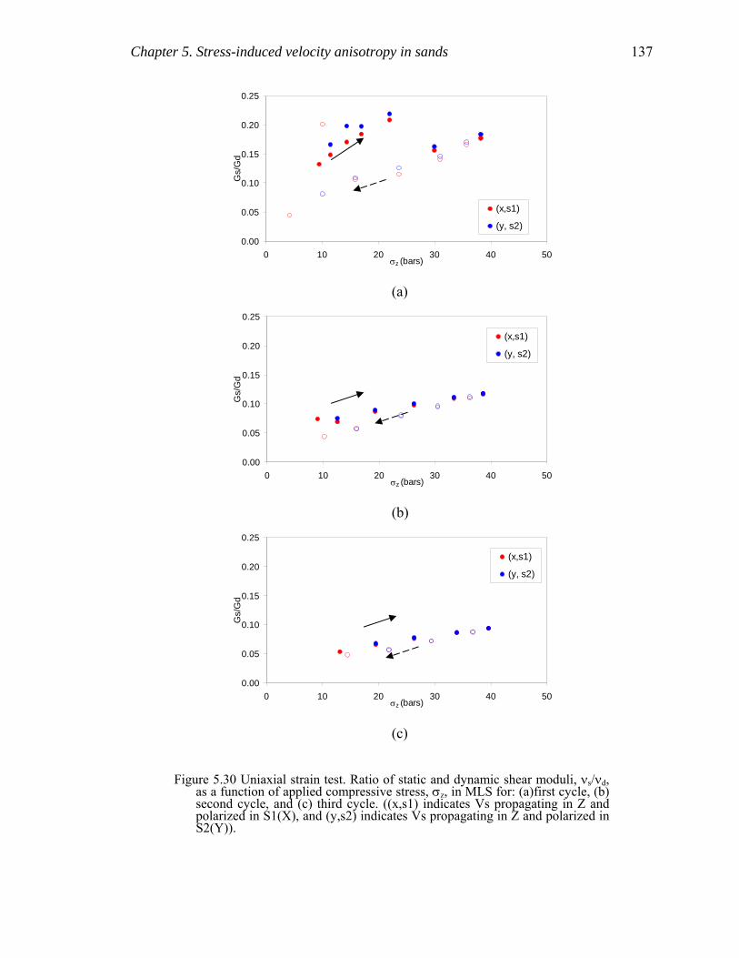
Chapter 5. Stress-induced velocity anisotropy in sands 137
(a)
(b)
(c)
Figure 5.30 Uniaxial strain test. Ratio of static and dynamic shear moduli, νs/νd,
as a function of applied compressive stress, σz, in MLS for: (a)first cycle, (b) second cycle, and (c) third cycle. ((x,s1) indicates Vs propagating in Z and polarized in S1(X), and (y,s2) indicates Vs propagating in Z and polarized in S2(Y)).
0.00
0.05
0.10
0.15
0.20
0.25
0 10 20 30 40 50σz (bars)
Gs/
Gd
(x,s1)
(y, s2)
0.00
0.05
0.10
0.15
0.20
0.25
0 10 20 30 40 50σz (bars)
Gs/
Gd
(x,s1)
(y, s2)
0.00
0.05
0.10
0.15
0.20
0.25
0 10 20 30 40 50σz (bars)
Gs/
Gd
(x,s1)
(y, s2)

138 Chapter 5. Stress-induced velocity anisotropy in sands
5.6 Conclusions I measured velocity anisotropy due to stress anisotropy in three different sands in a
higher compressive stress range (0-40 bars) than previous studies (0-8 bars). I found that
each separate sample displayed a linear dependence of velocity anisotropy with stress
anisotropy. This stress anisotropy was reduced if boundary effects were taking in account
using the approximation of a half space surface with an applied periodic normal stress. In
addition, Vp showed a steep slope at low applied compressive stress and a flatter slope at
higher compressive stress; most previous work has been done only at lower compressive
stresses. The results suggest that velocity anisotropy is more significantly affected by
stress anisotropy than by textural anisotropy. In addition, Vpz was slightly higher in the
coarse-grained sample than in the fine-grained sample as a result of grain size.
The strain showed hysteresis during loading and unloading for the sands, in
complement to previous studies, with larger value of strain for the coarse-grained sand
than for the fine-grained sand. This hysteresis corresponded to the stress accumulation in
the XY plane, due to overconsolidation, which also led to higher velocities in that plane
and lower velocity anisotropy. Future research will study the effect of grain size, packing,
and sorting on the strain, as well as on the velocity anisotropy behavior.
The Vp change with porosity was larger in the finer-grained sands than in the coarser-
grained sand. This result suggests that finer-grained sands present larger compaction than
coarser-grained sands. Nevertheless, the relation between grain size and compaction need
further research.
Vp frequencies seem to be related to stress anisotropy for velocity anisotropy higher
than 29%. Vp and Vs frequencies did not show correlation with stress-induced velocity
anisotropy in MLS, with the lowest ∆Vp.
The Norris and Johnson model for infinitely rough contacts predicts well Vpx and
Vpy as functions of applied compressive stress under uniaxial strain test in sands. The
Norris and Johnson model for infinitely smooth contacts and Makse’s correction more
accurately predicts Vpz as a function of applied compressive stress than does the model
with infinitely rough contacts. However, even the improvement prediction does not
match the experimental Vpz data well.

Chapter 5. Stress-induced velocity anisotropy in sands 139
Static and dynamic elastic constants in sands appear to be correlated. The correlations
for the first cycle and initial rearrangements differed from the correlations for latter
cycles with the same sample.
5.7 References Chang, C. T., 1998, Time-dependent deformation in unconsolidated reservoir sands:
Ph.D. thesis, Stanford University, Stanford, CA.
Cheng, C. H., and Johnston, D. H., 1981, Dynamic and static moduli: Geophysical
Research Letters, 8, 39-42.
Cizeau, P., Makse, H. A., and Stanley, E., 1999, Mechanisms of granular spontaneous
stratification and segregation in two-dimensional silos: Physical Review E, 59, 4408-
4421.
Dvorkin, K, and Nur, A., 1996, Elasticity of high porosity sandstones: Theory for two
North Sea datasets: Geophysics, 61, 1362-1370.
Finkbeiner, T., 1998, In situ stress, pore pressure, and hydrocarbon migration and
accumulation in sedimentary basins: Ph.D. thesis, Stanford University, Stanford, CA.
Fioravante, V., and Capoferri, R., 2001, On the use of multi-directional piezoelectric
transducers in triaxial testing: Geotechnical Testing Journal, 24, 243-255.
Jaeger, J. C., and Cook, N. G. W., 1979, Fundamentals of Rock Mechanics, Chapman
and Hall, London.
Jiang, G-L., Tatsuoka, F., Flora, A., and Koseki, J., 1997, Inherent and stress-state-
induced anisotropy in very small strain stiffness of a sand gravel: Geotechnique, 47,
509-521.
Johnson, D. L., Schwartz, L. M., Elata, D., Berryman, J.G., Hornby, B., and Norris, A.
N., 1998, Linear and nonlinear elasticity of granular media: stress-induced anisotropy
of a random sphere pack: Transactions of the ASME, 65, 380-388.
Makse, H. A., Gland, N., Johnson, D. L., Schwartz, L. M., 1999, Why effective medium
theory fails in granular materials: Physical Review Letter, 83, 5070-5073.
Mavko, G., Mukerji, T., and Godfrey, N., 1995, Predicting stress-induced velocity
anisotropy in rocks: Geophysics, 61, 1081-1087.
Mavko, G., Tapan, M., and Dvorkin, J., 1998, The Rock Physics Handbook: Cambridge
University Press, NY.

140 Chapter 5. Stress-induced velocity anisotropy in sands
Mayne, P., W., and Kulhawy, F., H., 1982, Ko-OCR relationships in soil: Geotechnical
Engineering Division, 108, 851-872.
Midndlin, R. D., 1949, Compliance of elastic bodies in contact: Journal of Applied
Mechanics, 16, 259-268.
Norris, A. N., and Johnson, D. L., 1997, Nonlinear elasticity of granular media: ASME
Journal of Applied Mechanics, 64, 39-49.
Nur, A. and Simmons, G., 1969, Stress-induced velocity anisotropy in rock: an
experimental study: Journal of Geophysical Research, 74, 6667-6674.
Nur, A., 1971, Effects of stress on velocity anisotropy in rocks with cracks: Journal of
Geophysical Research, 76, 2022-2034.
Prasad, M., and Meissner, R., 1992, Attenuation mechanisms in sands: Laboratory versus
theoretical (Biot) data: Geophysics, 57, 710-719.
Santamarina, J. C., and Cascante, G., 1996, Stress anisotropy and wave propagation: a
micromechanical view: Canadian Geotechnical Journal, 33, 770-782.
Santamarina, J. C., 2001, Soils and waves. Particulate materials behavior,
characterization and process monitoring: John Wiley and Sons, Ltd., West Sussex,
England.
Sinha, B. K. and Kostek, S., 1996, Stress-induced azimuthal anisotropy in borehole
flexural waves: Geophysics, 61, 1899-1907.
Sinha, B. K., and Plona, T. J., 2001, Wave propagation in rocks with elastic-plastic
deformations: Geophysics, 66, 772-785.
Sivakumar, V., Doran, I. G., Graham, J. and Navaneethan, T., 2001, Relationship
Between Ko and Overconsolidation Ratio - A Theoretical Approach: Geotechnique,
52, 225-230.
Walton, K., 1987, The effective elastic moduli of a random packing of spheres: Journal of
Mechanics and Physics of Solids, 35, 213-226.
Yin, H., 1993, Acoustic velocity and attenuation of rocks: isotropy, intrinsic anisotropy,
and stress-induced anisotropy: Ph.D. thesis, Stanford University, pp. 118-178,
Stanford, CA.
Zeng, X., 1999, Stress-induced anisotropic Gmax of sands and its measurements: Journal
of Geotechnical and Geoenvironmental Engineering, 125, 741-749.

143
Appendix A Data tables
Table A1. Uniaxial strain test (Chapter 5). Measured stress, velocity, and strain data of SCS (Santa Cruz sand, 0.45 of porosity, mean grain size of 0.25 mm, and 2.606 of grain density).
σz σx σy Vpz Vpx Vpy εz εx εy
bars bars bars m/s m/s m/s
9.2 0.9 0.6 0.051 -0.003 -0.004 3.8 0.4 0.3 489 327 295 0.051 -0.003 -0.004
15.8 1.8 1.3 0.054 -0.003 -0.006 8.8 1.2 0.9 578 402 360 0.054 -0.003 -0.006
24.5 3.0 2.3 0.057 -0.004 -0.006 15.9 2.2 1.8 664 447 428 0.057 -0.004 -0.007 25.6 3.4 2.5 0.058 -0.004 -0.007 20.7 2.8 2.2 702 468 449 0.058 -0.004 -0.007 28.7 4.0 2.9 0.058 -0.004 -0.007 24.4 3.4 2.7 728 484 461 0.058 -0.004 -0.007 33.3 4.8 3.4 0.059 -0.005 -0.007 28.2 4.0 3.0 747 502 473 0.059 -0.005 -0.007 37.9 5.5 3.8 0.060 -0.005 -0.008 31.8 4.7 3.5 763 519 491 0.060 -0.005 -0.008 40.4 5.9 4.1 0.061 -0.005 -0.008 34.6 5.2 3.8 782 524 497 0.061 -0.005 -0.008 49.3 7.1 5.0 0.062 -0.005 -0.008 40.5 6.1 4.5 807 542 524 0.062 -0.005 -0.008 35.0 5.0 4.0 0.062 -0.006 -0.008 34.9 5.1 4.1 787 531 518 0.062 -0.006 -0.008 31.3 4.9 3.9 0.062 -0.006 -0.008 31.4 5.0 3.9 773 526 514 0.062 -0.006 -0.008 27.1 4.6 3.7 0.062 -0.006 -0.008 27.3 4.6 3.7 743 519 502 0.062 -0.006 -0.008 23.2 4.3 3.5 0.062 -0.006 -0.008 23.6 4.3 3.5 732 515 496 0.062 -0.006 -0.008 19.1 4.0 3.2 0.062 -0.006 -0.008 19.6 3.9 3.2 699 509 492 0.062 -0.006 -0.008 15.4 3.6 3.0 0.062 -0.006 -0.008 15.9 3.6 2.9 657 491 473 0.062 -0.006 -0.008 11.5 3.1 2.5 0.062 -0.006 -0.008 12.0 3.0 2.5 622 473 459 0.062 -0.006 -0.008 7.6 2.5 2.0 0.062 -0.006 -0.008 8.2 2.5 2.0 556 449 432 0.062 -0.006 -0.008

144 Appendix A. Data tables
σz σx σy Vpz Vpx Vpy εz εx εy
bars bars bars m/s m/s m/s
4.2 1.7 1.4 0.061 -0.006 -0.008 4.6 1.7 1.4 478 405 393 0.061 -0.006 -0.008 2.0 1.1 0.8 0.061 -0.006 -0.007 2.4 1.1 0.8 387 358 348 0.061 -0.006 -0.007 0.1 0.1 0.1 0.056 -0.005 -0.007 0.1 0.1 0.1 0.055 -0.002 -0.006
Table A2. Uniaxial strain test (Chapter 5). Measured stress, velocity, and strain
data of MS (Monterrey sand, 0.41 of porosity, mean grain size of 0.91 mm, and 2.613 of grain density).
σz σx σy Vpz Vpx Vpy εz εx εy
bars bars bars m/s m/s m/s
3.9 0.3 0.4 0.017 0.000 -0.003 2.0 0.2 0.3 435 312 311 0.017 0.000 -0.003 5.9 0.3 0.6 0.020 0.001 -0.004 3.9 0.3 0.5 500 350 361 0.020 0.001 -0.004 11.7 0.9 1.4 0.023 0.012 -0.005 7.2 0.7 1.1 579 413 431 0.024 0.001 -0.005 15.6 1.6 2.0 0.025 0.001 -0.005 14.0 1.6 1.8 682 477 487 0.026 0.001 -0.005 20.8 2.2 2.4 0.027 0.005 -0.005 16.4 1.8 2.1 705 483 506 0.027 0.003 -0.005 23.4 2.5 2.8 0.028 0.000 -0.005 21.0 2.3 2.6 742 509 531 0.028 0.000 -0.005 27.3 3.0 3.2 0.029 0.000 -0.005 24.3 2.7 3.0 760 531 538 0.029 0.000 -0.005 31.2 3.7 3.7 0.030 0.000 -0.005 28.0 3.2 3.4 797 554 573 0.030 0.000 -0.005 35.1 4.4 4.2 0.031 0.000 -0.005 31.4 3.8 3.9 822 577 580 0.031 0.000 -0.005 39.0 5.3 4.8 0.033 0.000 -0.005 37.1 4.8 4.6 854 596 611 0.033 -0.001 -0.005 43.3 5.8 5.2 0.034 -0.001 -0.005 39.6 5.2 4.9 874 604 632 0.034 -0.001 -0.005 35.0 4.9 4.6 0.034 -0.001 -0.005 35.1 4.9 4.6 826 594 610 0.034 -0.001 -0.005 31.2 4.6 4.4 0.034 -0.001 -0.005 31.3 4.6 4.4 795 585 596 0.034 -0.001 -0.005 27.5 4.3 4.3 0.034 -0.001 -0.005 27.5 4.3 4.2 757 568 584 0.034 -0.001 -0.005 23.1 4.0 4.0 0.034 -0.001 -0.005 23.4 3.9 3.9 727 558 579 0.034 -0.001 -0.005

Appendix A. Data tables 145
σz σx σy Vpz Vpx Vpy εz εx εy
bars bars bars m/s m/s m/s
19.5 3.6 3.7 0.034 -0.001 -0.005 19.7 3.6 3.7 707 553 564 0.034 -0.001 -0.005 15.5 3.3 3.3 0.033 -0.001 -0.005 15.7 3.2 3.3 676 528 549 0.033 -0.001 -0.005 11.7 2.8 2.9 0.033 -0.001 -0.005 12.0 2.8 2.8 630 498 533 0.033 -0.001 -0.005 7.8 2.2 2.3 0.033 -0.001 -0.005 8.1 2.2 2.3 557 486 509 0.033 -0.001 -0.005 3.9 1.3 1.4 0.032 -0.001 -0.005 4.2 1.4 1.4 457 444 464 0.032 -0.001 -0.005 2.3 0.8 0.9 0.031 -0.001 -0.004 2.6 0.9 0.9 393 406 426 0.031 -0.001 -0.004 0.1 0.1 0.1 0.023 -0.002
Table A3. Uniaxial strain test (Chapter 5). Measured stress, velocity, and strain
data of MLS (Moss Landing sand, 0.42 of porosity, mean grain size of 0.39 mm, and 2.629 of grain density).
σz σx σy Vpz Vs1z Vs2z Vpx Vs1x Vs2x Vpy Vs1y Vs2y εz εx εy
bars bars bars m/s m/s m/s m/s m/s m/s m/s m/s m/s
0.0 0.0 0.0 135 149 0.002 0.006 0.010 2.3 0.1 0.2 0.045 -
0.001 0.002
1.5 0.1 0.1 286 216 243 0.045 -0.002
0.002
4.7 0.2 0.3 0.045 -0.004
-0.002
3.9 0.2 0.2 399 291 321 0.045 -0.004
-0.002
6.6 0.4 0.4 0.045 -0.006
-0.004
5.7 0.3 0.4 464 332 362 0.045 -0.006
-0.004
8.9 0.4 0.8 0.055 -0.009
-0.007
7.7 0.4 0.6 495 342 390 0.055 -0.009
-0.007
10.7 0.6 0.9 0.056 -0.010
-0.008
9.4 0.5 0.7 525 336 368 417 0.056 -0.010
-0.007
12.7 0.8 1.2 0.056 -0.011
-0.008
11.4 0.7 1.1 558 347 328 394 437 0.056 -0.011
-0.008
16.1 1.1 1.6 0.056 -0.012
-0.009
14.4 1.0 1.4 605 364 338 426 469 0.056 -0.012
-0.010
19.3 1.2 2.1 0.056 -0.013
-0.011
17.0 1.2 1.8 634 380 367 451 314 505 0.056 -0.013
-0.011

146 Appendix A. Data tables
σz σx σy Vpz Vs1z Vs2z Vpx Vs1x Vs2x Vpy Vs1y Vs2y εz εx εy
bars bars bars m/s m/s m/s m/s m/s m/s m/s m/s m/s
24.3 1.8 2.8 0.056 -0.015
-0.012
22.0 1.8 2.5 674 404 394 509 352 541 274 350 0.056 -0.015
-0.012
33.7 3.1 4.1 0.063 -0.016
-0.014
30.0 2.9 3.7 757 431 422 556 283 368 594 309 362 0.063 -0.016
-0.014
41.7 4.4 5.6 0.063 -0.018
-0.016
38.2 4.2 5.2 810 452 444 627 302 396 637 336 383 0.063 -0.018
-0.016
35.7 4.1 4.9 807 451 445 638 301 395 626 333 381 0.063 -
0.018 -
0.016 31.0 3.7 4.6 0.064 -
0.018 -
0.016 31.0 3.7 4.6 792 441 434 622 297 391 619 301 378 0.064 -
0.018 -
0.016 23.6 3.2 4.3 0.064 -
0.018 -
0.016 23.6 3.1 4.3 744 422 403 585 288 377 601 272 344 0.064 -
0.018 -
0.016 15.7 2.5 3.4 0.063 -
0.017 -
0.015 15.9 2.5 3.4 663 358 353 547 277 355 573 330 0.063 -
0.018 -
0.015 9.9 1.8 2.5 0.063 -
0.017 -
0.015 10.1 1.8 2.5 584 327 324 501 330 533 312 0.063 -
0.017 -
0.015 5.8 1.2 1.6 0.062 -
0.016 -
0.014 6.0 1.2 1.6 469 451 440 0.062 -
0.016 -
0.014 4.0 0.9 1.1 0.062 -
0.016 -
0.014 4.2 0.8 1.1 406 287 410 436 0.062 -
0.016 -
0.014 2.1 0.4 0.5 0.061 -
0.015 -
0.013 2.3 0.4 0.5 312 349 368 0.061 -
0.015 -
0.013 1.4 0.2 0.2 0.061 -
0.015 -
0.013 1.5 0.2 0.2 245 301 307 0.061 -
0.015 -
0.013 0.0 0.1 0.0 0.056 -
0.008 -
0.005 0.1 0.1 0.0 114 165 177 0.056 -
0.008 -
0.005
0.1 0.2 0.0 113 171 188 0.055 -0.007
-0.003
3.0 0.3 0.2 0.063 -0.010
-0.008
2.2 0.2 0.1 340 296 287 0.063 -0.010
-0.008
5.0 0.5 0.4 0.063 -0.012
-0.010
4.2 0.4 0.3 421 331 346 0.063 -0.012
-0.010
10.3 0.9 0.9 0.063 - -

Appendix A. Data tables 147
σz σx σy Vpz Vs1z Vs2z Vpx Vs1x Vs2x Vpy Vs1y Vs2y εz εx εy
bars bars bars m/s m/s m/s m/s m/s m/s m/s m/s m/s
0.014 0.013 9.0 0.9 0.9 542 341 396 0 0.063 0.070 0.066
14.1 1.3 1.5 0.063 -0.015
-0.014
12.6 1.2 1.4 601 364 350 425 315 475 0.069 -0.015
-0.014
21.4 1.9 2.8 0.069 -0.017
-0.016
19.4 1.8 2.5 687 395 389 490 253 322 541 238 310 0.069 -0.017
-0.016
29.2 2.7 4.3 0.071 -0.018
-0.017
26.3 2.6 3.9 749 420 414 524 278 362 585 288 358 0.071 -0.018
-0.017
36.3 3.7 5.7 0.071 -0.019
-0.018
33.4 3.6 5.2 802 439 434 566 293 387 603 300 380 0.071 -0.019
-0.018
42.1 4.5 6.6 0.072 -0.020
-0.019
38.6 4.4 6.0 831 451 449 598 306 402 642 313 400 0.072 -0.020
-0.019
36.2 4.2 5.8 843 450 446 603 306 403 645 313 397 0.072 -
0.020 -
0.019 30.4 4.0 5.0 0.072 -
0.020 -
0.019 30.5 4.0 5.0 799 442 437 597 302 394 634 311 388 0.072 -
0.020 -
0.019 23.8 3.6 4.6 0.072 -
0.020 -
0.019 24.0 3.6 4.6 753 423 418 582 294 384 609 298 377 0.072 -
0.020 -
0.019 15.9 2.8 3.9 0.072 -
0.019 -
0.019 16.0 2.8 3.9 681 395 399 555 279 362 576 249 320 0.072 -
0.019 -
0.019 10.0 2.2 2.7 0.071 -
0.019 -
0.018 10.3 2.2 2.7 586 360 512 256 339 538 0.071 -
0.019 -
0.018 5.9 1.6 1.7 0.071 -
0.018 -
0.018 6.1 1.5 1.7 501 464 192 318 490 0.071 -
0.018 -
0.018 4.1 1.1 1.3 0.070 -
0.018 -
0.017 4.3 1.0 1.2 420 422 181 290 445 0.070 -
0.018 -
0.017 2.2 0.5 0.7 0.070 -
0.017 -
0.017
1.3 0.3 0.3 0.069 -0.016
-0.016
1.5 0.3 0.4 258 304 314 0.069 -0.016
-0.016
0.1 0.1 0.0 0.065 -0.011
-0.009
0.1 0.1 0.0 67 170 187 0.063 -0.010
-0.007
0.1 0.1 0.0 87 173 187 0.062 - -

148 Appendix A. Data tables
σz σx σy Vpz Vs1z Vs2z Vpx Vs1x Vs2x Vpy Vs1y Vs2y εz εx εy
bars bars bars m/s m/s m/s m/s m/s m/s m/s m/s m/s
0.009 0.006 3.0 0.3 0.2 0.072 -
0.013 -
0.011 2.1 0.2 0.1 327 298 294 0.072 -
0.013 -
0.011 5.1 0.5 0.4 0.073 -
0.014 -
0.013 4.4 0.5 0.4 428 342 346 0.073 -
0.014 -
0.013 10.7 1.1 1.2 0.075 -
0.016 -
0.015 9.3 1.0 1.1 564 408 435 0.075 -
0.016 -
0.016 14.5 1.6 1.8 0.075 -
0.017 -
0.016 13.1 1.4 1.7 625 369 442 293 473 0.075 -
0.017 -
0.016 21.4 2.1 3.0 0.077 -
0.018 -
0.018 19.5 2.0 2.7 706 398 393 492 255 319 511 319 0.077 -
0.018 -
0.018 28.8 2.7 4.3 0.078 -
0.019 -
0.018 26.4 2.6 4.0 755 422 418 527 277 339 574 222 358 0.078 -
0.019 -
0.019 36.9 3.7 5.6 0.078 -
0.020 -
0.019 34.0 3.7 5.2 835 444 442 574 293 365 626 268 388 0.078 -
0.020 -
0.019 42.8 4.7 6.4 0.079 -
0.021 -
0.020 39.6 4.6 6.1 870 455 454 608 312 380 656 303 403 0.079 -
0.021 -
0.020
36.8 4.4 5.7 852 454 453 598 311 380 644 302 402 0.079 -0.021
-0.020
29.3 4.2 5.2 0.079 -0.021
-0.020
29.5 4.1 5.2 808 442 441 616 305 369 631 299 396 0.079 -0.021
-0.020
21.7 3.6 4.7 0.079 -0.021
-0.020
21.9 3.6 4.7 749 419 424 587 295 353 606 382 0.079 -0.021
-0.020
14.2 2.8 3.9 0.079 -0.020
-0.020
14.4 2.8 3.9 681 363 550 279 333 568 249 347 0.079 -0.020
-0.020
9.2 2.1 3.0 0.078 -0.020
-0.019
9.4 2.1 3.0 594 510 249 308 524 324 0.078 -0.020
-0.019
6.1 1.5 2.2 0.078 -0.019
-0.019
6.4 1.5 2.2 509 463 226 293 482 0.078 -0.019
-0.019
4.1 1.1 1.7 0.077 -0.019
-0.019
4.3 1.1 1.6 453 423 212 279 441 0.077 -0.019
-0.019
2.1 0.7 0.8 0.076 -0.018
-0.018
2.3 0.6 0.8 335 370 377 0.076 - -

Appendix A. Data tables 149
σz σx σy Vpz Vs1z Vs2z Vpx Vs1x Vs2x Vpy Vs1y Vs2y εz εx εy
bars bars bars m/s m/s m/s m/s m/s m/s m/s m/s m/s
0.018 0.018 1.3 0.4 0.4 0.076 -
0.017 -
0.017 1.4 0.4 0.4 255 319 317 0.076 -
0.017 -
0.017 0.2 0.1 0.1 0.071 -
0.012 -
0.010 0.2 0.1 0.1 83 191 189 0.071 -
0.011 -
0.009 0.2 0.1 0.1 0.071 -
0.011 -
0.009 Table A4. Quasi-hydrostatic stress test (Chapter 3 and 4). Measured stress,
velocity, and strain data of QNS1 (poured Santa Cruz Sand, 0.48 of porosity, mean grain size of 0.25 mm, and 2.606 of grain density, loading order: Z X
Y).
σz σx σy Vpz Vpx Vpy εz εx εy
bars bars bars m/s m/s m/s
0.1 0.1 0.0 185 134 72 0.009 0.009 0.001 3.3 3.0 3.0 0.018 0.037 -0.011 2.3 2.4 2.1 408 487 488 0.018 0.036 -0.012 4.6 4.5 4.6 0.018 0.038 -0.010 4.1 4.2 4.0 462 574 573 0.018 0.038 -0.010 8.3 8.2 8.0 0.019 0.040 -0.007 7.1 7.2 6.7 528 662 650 0.019 0.040 -0.007
13.3 13.2 13.1 0.020 0.041 -0.003 11.7 11.4 11.3 600 738 728 0.020 0.041 -0.003 17.8 17.6 17.8 0.020 0.043 0.000 16.0 15.8 15.5 648 794 793 0.020 0.042 0.000 21.0 21.3 21.3 0.020 0.043 0.002 19.5 19.9 19.3 696 838 848 0.020 0.043 0.002 24.4 24.3 24.7 0.020 0.044 0.003 22.9 22.8 22.6 705 878 879 0.020 0.044 0.003 29.1 29.2 29.5 0.021 0.045 0.006 27.3 27.4 27.1 735 915 923 0.021 0.045 0.006 32.7 33.1 32.8 0.021 0.046 0.007 30.6 30.8 30.0 759 952 963 0.021 0.046 0.007 36.1 36.9 36.9 0.021 0.047 0.008 34.2 34.9 34.1 782 985 1000 0.021 0.047 0.008 40.9 41.2 41.1 0.021 0.048 0.009 38.9 39.0 38.0 814 1016 1035 0.021 0.048 0.009
37.1 37.5 36.4 821 1012 1036 0.021 0.047 0.009 32.3 30.9 32.1 0.021 0.047 0.009
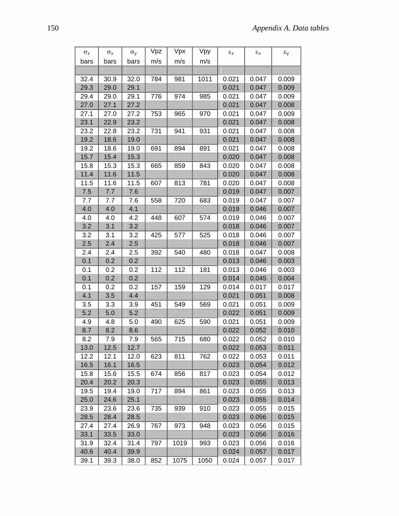
150 Appendix A. Data tables
σz σx σy Vpz Vpx Vpy εz εx εy
bars bars bars m/s m/s m/s
32.4 30.9 32.0 784 981 1011 0.021 0.047 0.009 29.3 29.0 29.1 0.021 0.047 0.009 29.4 29.0 29.1 776 974 985 0.021 0.047 0.009 27.0 27.1 27.2 0.021 0.047 0.008 27.1 27.0 27.2 753 965 970 0.021 0.047 0.009 23.1 22.9 23.2 0.021 0.047 0.008 23.2 22.8 23.2 731 941 931 0.021 0.047 0.008 19.2 18.6 19.0 0.021 0.047 0.008 19.2 18.6 19.0 691 894 891 0.021 0.047 0.008 15.7 15.4 15.3 0.020 0.047 0.008 15.8 15.3 15.3 665 859 843 0.020 0.047 0.008 11.4 11.6 11.5 0.020 0.047 0.008 11.5 11.6 11.5 607 813 781 0.020 0.047 0.008 7.5 7.7 7.6 0.019 0.047 0.007 7.7 7.7 7.6 558 720 683 0.019 0.047 0.007 4.0 4.0 4.1 0.019 0.046 0.007 4.0 4.0 4.2 448 607 574 0.019 0.046 0.007 3.2 3.1 3.2 0.018 0.046 0.007 3.2 3.1 3.2 425 577 525 0.018 0.046 0.007 2.5 2.4 2.5 0.018 0.046 0.007 2.4 2.4 2.5 392 540 480 0.018 0.047 0.008 0.1 0.2 0.2 0.013 0.046 0.003 0.1 0.2 0.2 112 112 181 0.013 0.046 0.003 0.1 0.2 0.2 0.014 0.045 0.004 0.1 0.2 0.2 157 159 129 0.014 0.017 0.017 4.1 3.5 4.4 0.021 0.051 0.008 3.5 3.3 3.9 451 549 569 0.021 0.051 0.009 5.2 5.0 5.2 0.022 0.051 0.009 4.9 4.8 5.0 490 625 590 0.021 0.051 0.009 8.7 8.2 8.6 0.022 0.052 0.010 8.2 7.9 7.9 565 715 680 0.022 0.052 0.010
13.0 12.5 12.7 0.022 0.053 0.011 12.2 12.1 12.0 623 811 762 0.022 0.053 0.011 16.5 16.1 16.5 0.023 0.054 0.012 15.8 15.6 15.5 674 856 817 0.023 0.054 0.012 20.4 20.2 20.3 0.023 0.055 0.013 19.5 19.4 19.0 717 894 861 0.023 0.055 0.013 25.0 24.6 25.1 0.023 0.055 0.014 23.9 23.6 23.6 735 939 910 0.023 0.055 0.015 28.5 28.4 28.5 0.023 0.056 0.015 27.4 27.4 26.9 767 973 948 0.023 0.056 0.015 33.1 33.5 33.0 0.023 0.056 0.016 31.9 32.4 31.4 797 1019 993 0.023 0.056 0.016 40.6 40.4 39.9 0.024 0.057 0.017 39.1 39.3 38.0 852 1075 1050 0.024 0.057 0.017

Appendix A. Data tables 151
σz σx σy Vpz Vpx Vpy εz εx εy
bars bars bars m/s m/s m/s
37.8 38.2 36.6 840 1075 1053 0.024 0.058 0.017 29.4 28.4 29.3 0.024 0.057 0.017 29.4 28.4 29.2 794 1008 988 0.023 0.057 0.017 21.1 20.7 21.3 0.023 0.057 0.017 21.2 20.7 21.3 735 943 912 0.023 0.057 0.017 19.0 18.6 18.8 0.023 0.057 0.016 19.0 18.6 18.9 732 913 894 0.023 0.057 0.016 13.7 13.6 13.7 0.023 0.057 0.015 13.7 13.5 13.7 686 851 813 0.023 0.056 0.015 9.4 9.6 9.5 0.022 0.055 0.015 9.4 9.6 9.5 623 784 719 0.022 0.055 0.015 5.8 5.7 5.9 0.022 0.055 0.014 5.7 5.7 5.9 529 695 631 0.022 0.055 0.015 3.8 3.7 3.8 0.021 0.055 0.014 3.7 3.7 3.8 454 617 550 0.021 0.055 0.014 2.7 2.7 2.7 0.021 0.055 0.014 2.6 2.7 2.7 414 565 501 0.021 0.055 0.014 1.5 1.6 1.6 0.020 0.054 0.013 1.4 1.6 1.6 350 475 383 0.020 0.054 0.013 0.5 0.5 0.5 0.019 0.054 0.009 0.5 0.6 0.5 263 338 209 0.019 0.054 0.010 0.1 0.2 0.2 0.018 0.050 0.009 0.1 0.2 0.2 0.018 0.048 0.009 2.3 2.0 2.3 0.025 0.049 0.011 1.9 1.9 2.0 387 462 444 0.025 0.049 0.011 4.3 3.9 4.2 0.025 0.057 0.013 3.9 3.7 3.9 486 594 574 0.025 0.057 0.012 8.8 8.0 8.7 0.026 0.059 0.014 8.2 7.8 8.2 596 724 695 0.026 0.059 0.014
25.2 23.9 25.2 0.027 0.062 0.017 23.9 23.1 23.7 778 942 926 0.027 0.063 0.017 39.6 39.5 39.4 0.028 0.064 0.019 37.5 37.9 36.8 913 1095 1053 0.028 0.065 0.019 43.9 43.9 44.3 0.029 0.065 0.018 41.2 41.6 38.1 921 1110 1053 0.029 0.065 0.019 48.1 49.4 48.3 0.029 0.065 0.019 47.0 48.1 46.4 919 1153 1097 0.029 0.065 0.020 32.5 32.1 32.3 0.028 0.065 0.019 32.6 32.1 32.3 860 1050 1039 0.028 0.065 0.020 24.8 24.2 24.8 0.028 0.064 0.019 24.8 24.2 24.9 797 981 973 0.028 0.064 0.018 8.9 8.3 9.1 0.026 0.063 0.018 8.8 8.3 9.0 638 764 715 0.026 0.063 0.018 5.0 4.8 5.1 0.025 0.063 0.017

152 Appendix A. Data tables
σz σx σy Vpz Vpx Vpy εz εx εy
bars bars bars m/s m/s m/s
4.8 4.7 5.1 556 662 618 0.025 0.063 0.018 2.6 2.4 2.7 0.024 0.063 0.017 2.5 2.4 2.7 410 538 500 0.024 0.063 0.017 0.9 1.0 1.1 0.022 0.062 0.017 0.9 1.0 1.1 294 396 304 0.022 0.062 0.017 0.1 0.2 0.2 0.020 0.057 0.012 0.0 0.1 0.2 0.023 0.055 0.011 0.0 0.1 0.2 0.023 0.054 0.011 0.0 0.1 0.1 0.023 0.053 0.011 0.0 0.1 0.1 0.023 0.053 0.011
Table A5. Quasi-hydrostatic stress test (Chapter 3). Measured stress, velocity,
and strain data of QNS2 (poured Santa Cruz Sand, 0.47 of porosity, mean grain size of 0.25 mm, and 2.606 of grain density, loading order: X Y Z).
σz σx σy Vpz Vpx Vpy εz εx εy bars bars bars m/s m/s m/s
0.1 0.1 0.0 0.003 0.006 0.005
0.0 0.1 0.0 193 145 143 0.003 0.005 0.006 0.4 0.5 0.5 0.001 0.019 0.011 0.2 0.4 0.3 234 268 257 0.001 0.019 0.011 1.6 1.8 1.6 0.001 0.027 0.013 1.1 1.5 1.2 340 410 387 0.001 0.027 0.012 3.6 3.7 3.5 0.002 0.033 0.014 2.4 3.1 2.6 417 535 482 0.002 0.033 0.014 5.6 5.8 5.3 0.003 0.035 0.016 4.3 5.2 4.4 468 613 574 0.003 0.035 0.016 7.8 7.6 7.4 0.003 0.037 0.017 6.4 7.0 6.3 514 663 619 0.003 0.037 0.020 9.5 9.3 9.2 0.003 0.039 0.021 8.2 8.8 8.2 544 710 661 0.003 0.039 0.020
13.1 12.9 12.8 0.004 0.040 0.022 11.5 12.1 11.5 593 764 734 0.004 0.040 0.022 16.8 16.8 16.5 0.004 0.042 0.023 15.2 16.0 15.1 620 819 787 0.004 0.042 0.023 21.1 21.1 20.9 0.004 0.045 0.026 19.0 19.9 19.1 664 868 827 0.004 0.045 0.026 25.3 25.0 24.9 0.004 0.047 0.027 23.4 24.0 23.2 712 908 878 0.004 0.047 0.027 29.2 29.3 29.2 0.004 0.047 0.028

Appendix A. Data tables 153
σz σx σy Vpz Vpx Vpy εz εx εy bars bars bars m/s m/s m/s
27.2 28.1 27.3 739 951 905 0.004 0.047 0.028 33.1 33.2 32.9 0.005 0.049 0.030 31.1 31.9 31.1 768 994 938 0.005 0.049 0.030 37.0 37.4 36.9 0.005 0.049 0.031 34.8 35.9 34.8 778 1022 965 0.005 0.049 0.031 41.2 40.9 40.9 0.005 0.050 0.032 38.8 39.5 38.8 803 1057 994 0.005 0.050 0.032
36.6 37.7 36.8 799 1051 984 0.005 0.050 0.032 32.6 32.6 32.0 0.005 0.050 0.030 32.5 32.6 32.0 779 1007 955 0.005 0.050 0.030 29.1 29.2 28.8 0.005 0.050 0.030 29.1 29.2 28.9 763 982 944 0.005 0.050 0.030 24.8 24.2 24.5 0.004 0.049 0.030 24.9 24.2 24.5 727 956 906 0.004 0.049 0.030 19.9 19.4 19.4 0.004 0.049 0.030 19.9 19.4 19.5 693 895 850 0.004 0.049 0.029 17.6 17.2 17.3 0.004 0.049 0.029 17.6 17.2 17.4 683 876 831 0.004 0.049 0.029 13.6 13.1 13.5 0.004 0.049 0.028 13.6 13.1 13.5 643 819 793 0.004 0.049 0.028 9.5 17.1 17.1 0.003 0.048 0.027 9.5 9.3 9.4 591 741 706 0.003 0.048 0.026 5.5 5.4 5.5 0.002 0.048 0.026 5.6 5.4 5.6 546 626 608 0.002 0.048 0.026 3.6 3.4 3.5 0.002 0.047 0.025 3.6 3.4 3.5 471 530 517 0.002 0.002 0.002 2.3 2.3 2.2 0.001 0.047 0.025 2.4 2.3 2.2 414 470 440 0.001 0.047 0.025 1.2 1.1 1.2 0.001 0.046 0.024 1.2 1.2 1.2 340 343 340 0.001 0.046 0.025 0.4 0.4 0.4 0.001 0.041 0.022 0.4 0.4 0.5 230 174 166 0.001 0.041 0.022 0.0 0.2 0.2 0.003 0.038 0.019 0.0 0.2 0.2 0.003 0.034 0.019 0.0 0.2 0.1 0.003 0.034 0.017 0.0 0.1 0.0 0.004 0.034 0.017 0.6 0.7 0.7 0.004 0.047 0.022 0.4 0.6 0.5 303 296 285 0.004 0.047 0.022 1.8 1.9 1.8 0.004 0.049 0.024 1.5 1.8 1.7 386 456 422 0.004 0.049 0.024 3.6 3.8 3.7 0.004 0.051 0.025 3.0 3.7 3.5 447 571 522 0.004 0.051 0.025 5.6 5.8 5.7 0.004 0.052 0.027 4.9 5.6 5.4 493 644 586 0.004 0.052 0.027
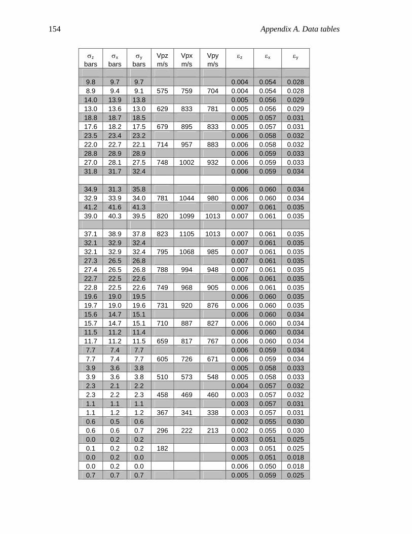
154 Appendix A. Data tables
σz σx σy Vpz Vpx Vpy εz εx εy bars bars bars m/s m/s m/s
9.8 9.7 9.7 0.004 0.054 0.028 8.9 9.4 9.1 575 759 704 0.004 0.054 0.028
14.0 13.9 13.8 0.005 0.056 0.029 13.0 13.6 13.0 629 833 781 0.005 0.056 0.029 18.8 18.7 18.5 0.005 0.057 0.031 17.6 18.2 17.5 679 895 833 0.005 0.057 0.031 23.5 23.4 23.2 0.006 0.058 0.032 22.0 22.7 22.1 714 957 883 0.006 0.058 0.032 28.8 28.9 28.9 0.006 0.059 0.033 27.0 28.1 27.5 748 1002 932 0.006 0.059 0.033 31.8 31.7 32.4 0.006 0.059 0.034
34.9 31.3 35.8 0.006 0.060 0.034 32.9 33.9 34.0 781 1044 980 0.006 0.060 0.034 41.2 41.6 41.3 0.007 0.061 0.035 39.0 40.3 39.5 820 1099 1013 0.007 0.061 0.035
37.1 38.9 37.8 823 1105 1013 0.007 0.061 0.035 32.1 32.9 32.4 0.007 0.061 0.035 32.1 32.9 32.4 795 1068 985 0.007 0.061 0.035 27.3 26.5 26.8 0.007 0.061 0.035 27.4 26.5 26.8 788 994 948 0.007 0.061 0.035 22.7 22.5 22.6 0.006 0.061 0.035 22.8 22.5 22.6 749 968 905 0.006 0.061 0.035 19.6 19.0 19.5 0.006 0.060 0.035 19.7 19.0 19.6 731 920 876 0.006 0.060 0.035 15.6 14.7 15.1 0.006 0.060 0.034 15.7 14.7 15.1 710 887 827 0.006 0.060 0.034 11.5 11.2 11.4 0.006 0.060 0.034 11.7 11.2 11.5 659 817 767 0.006 0.060 0.034 7.7 7.4 7.7 0.006 0.059 0.034 7.7 7.4 7.7 605 726 671 0.006 0.059 0.034 3.9 3.6 3.8 0.005 0.058 0.033 3.9 3.6 3.8 510 573 548 0.005 0.058 0.033 2.3 2.1 2.2 0.004 0.057 0.032 2.3 2.2 2.3 458 469 460 0.003 0.057 0.032 1.1 1.1 1.1 0.003 0.057 0.031 1.1 1.2 1.2 367 341 338 0.003 0.057 0.031 0.6 0.5 0.6 0.002 0.055 0.030 0.6 0.6 0.7 296 222 213 0.002 0.055 0.030 0.0 0.2 0.2 0.003 0.051 0.025 0.1 0.2 0.2 182 0.003 0.051 0.025 0.0 0.2 0.0 0.005 0.051 0.018 0.0 0.2 0.0 0.006 0.050 0.018 0.7 0.7 0.7 0.005 0.059 0.025

Appendix A. Data tables 155
σz σx σy Vpz Vpx Vpy εz εx εy bars bars bars m/s m/s m/s
0.5 0.6 0.5 314 307 286 0.005 0.059 0.025 1.8 2.0 1.8 0.005 0.061 0.027 1.5 1.9 1.7 398 477 419 0.005 0.061 0.027 3.7 3.9 3.7 0.005 0.062 0.028 3.2 3.8 3.5 461 601 538 0.005 0.062 0.028 5.7 5.9 5.7 0.006 0.063 0.030 5.2 5.8 5.4 511 691 609 0.006 0.063 0.030 9.6 9.9 9.6 0.006 0.065 0.031 8.8 9.7 9.2 573 794 701 0.006 0.065 0.031
13.9 14.5 14.0 0.007 0.066 0.033 12.8 14.0 13.4 633 879 789 0.007 0.066 0.033 19.7 20.3 19.5 0.007 0.067 0.034 18.3 19.7 18.7 691 959 856 0.007 0.067 0.034 27.2 28.0 27.2 0.007 0.068 0.036 25.5 27.3 26.1 738 1036 926 0.008 0.068 0.036 40.6 41.2 40.3 0.008 0.071 0.038 38.2 40.1 38.8 799 1114 1018 0.008 0.071 0.038
36.3 39.1 37.3 807 1114 1019 0.008 0.071 0.038 30.6 30.2 30.4 0.008 0.070 0.038 30.5 30.2 30.4 815 1048 979 0.008 0.070 0.038 21.2 19.9 20.7 0.008 0.070 0.038 21.4 19.9 20.8 736 954 907 0.008 0.070 0.038 17.3 16.6 17.1 0.008 0.069 0.037 17.4 16.7 17.2 697 909 862 0.008 0.070 0.037 13.4 13.0 13.2 0.008 0.069 0.037 13.6 13.0 13.3 673 857 807 0.008 0.069 0.037 9.8 20.8 21.2 0.008 0.069 0.036 9.9 9.1 9.6 620 789 735 0.008 0.069 0.036 5.9 5.3 5.7 0.007 0.069 0.035 5.9 5.3 5.7 552 674 645 0.007 0.069 0.035 2.8 2.8 3.0 0.006 0.068 0.035 2.8 2.8 3.0 461 548 532 0.006 0.068 0.035 1.8 2.0 2.0 0.005 0.068 0.034 1.9 2.0 2.0 410 450 432 0.005 0.068 0.034 0.6 0.5 0.7 0.005 0.064 0.032 0.6 0.6 0.7 299 233 242 0.005 0.064 0.032 0.1 0.2 0.1 0.006 0.060 0.022 0.1 0.2 0.1 184 0.006 0.060 0.022 0.0 0.2 0.0 0.006 0.059 0.020 0.0 0.0 0.0 179 0.006 0.057 0.017

156 Appendix A. Data tables
Table A6. Quasi-hydrostatic stress test (Chapter 3 and 4). Measured stress, velocity, and strain data of SCR (poured and rotated Santa Cruz Sand, 0.47 of porosity, mean grain size of 0.25 mm, and 2.606 of grain density, loading order: Z X Y).
σz σx σy Vpz Vpx Vpy εz εx εy bars bars bars m/s m/s m/s
0.0 0.0 0.0 0.004 0.004 0.003 0.2 0.2 0.2 0.004 0.004 0.003 0.1 0.2 0.2 113 180 0.003 0.004 0.004 0.6 0.6 0.5 0.025 0.006 0.004 0.4 0.5 0.3 270 306 276 0.025 0.007 0.005 1.7 1.7 1.6 0.029 0.009 0.004 1.3 1.4 1.1 389 443 405 0.029 0.009 0.004 3.5 3.4 3.3 0.032 0.011 0.005 2.8 2.8 2.5 491 559 505 0.032 0.011 0.005 5.4 5.3 5.4 0.033 0.012 0.006 4.6 4.6 4.3 567 638 589 0.033 0.013 0.006 9.0 8.9 8.9 0.034 0.014 0.006 8.2 7.8 7.3 663 738 669 0.034 0.014 0.007
13.4 13.1 13.7 0.035 0.016 0.007 12.4 11.9 11.7 730 833 749 0.034 0.016 0.008 17.4 17.9 17.8 0.035 0.016 0.008 16.2 16.2 15.3 783 901 806 0.035 0.016 0.009 24.5 24.6 25.2 0.017 0.010 22.7 22.6 22.1 861 985 880 0.036 0.017 0.010 33.6 34.0 34.4 0.037 0.018 0.010 31.8 31.7 30.6 965 1110 962 0.037 0.018 0.013 42.3 43.5 44.2 0.084 0.052 0.035 39.9 40.5 39.2 1005 1159 1015 0.079 0.004 -0.046
38.1 39.2 37.5 993 1153 1012 0.034 0.020 0.014
37.7 38.7 37.2 1010 1160 1001 0.034 0.020 0.014 29.2 28.7 29.3 0.034 0.020 0.014 29.2 28.8 29.2 924 1078 966 0.034 0.020 0.014 22.2 21.5 22.2 0.034 0.019 0.013 22.2 21.6 22.2 875 998 898 0.034 0.019 0.013 17.1 17.0 17.0 0.034 0.019 0.013 17.1 17.0 17.2 846 950 855 0.034 0.019 0.013 11.8 11.7 11.9 0.034 0.019 0.013 11.8 11.7 11.9 739 881 774 0.034 0.019 0.013 8.0 7.9 8.0 0.033 0.019 0.012 8.0 7.9 8.0 661 801 702 0.033 0.019 0.012 4.2 4.3 4.1 0.032 0.018 0.011 4.2 4.3 4.2 556 667 590 0.032 0.018 0.012 2.8 2.7 2.6 0.032 0.018 0.011 2.8 2.8 2.7 468 579 515 0.032 0.018 0.011

Appendix A. Data tables 157
σz σx σy Vpz Vpx Vpy εz εx εy bars bars bars m/s m/s m/s
1.5 1.5 1.6 0.031 0.017 0.011 1.5 1.5 1.6 367 447 440 0.031 0.017 0.011 0.5 0.6 0.6 0.031 0.016 0.011 0.6 0.6 0.7 276 267 286 0.031 0.016 0.011 0.2 0.3 0.2 0.031 0.012 0.011 0.2 0.3 0.3 161 97 192 0.031 0.012 0.011 0.1 0.2 0.0 0.030 0.008 0.010
0.0 0.2 0.3 0.030 0.008 0.010
0.7 0.7 0.7 0.042 0.013 0.010 0.4 0.6 0.6 265 286 278 0.042 0.013 0.010 2.0 2.0 2.0 0.043 0.016 0.010 1.5 1.8 1.6 411 474 424 0.042 0.016 0.010 4.1 4.1 4.1 0.043 0.018 0.011 3.4 3.8 3.6 552 635 557 0.043 0.018 0.011 6.4 6.2 6.3 0.042 0.019 0.011 5.6 5.9 5.7 623 712 636 0.042 0.019 0.012
10.2 9.6 10.0 0.043 0.020 0.012 9.3 9.2 8.9 706 802 706 0.043 0.020 0.012
14.4 13.9 14.0 0.043 0.021 0.013 13.5 13.4 12.8 776 892 777 0.043 0.021 0.013 18.2 18.2 17.9 0.043 0.022 0.014 17.2 17.2 16.3 834 955 839 0.043 0.022 0.014 25.3 25.1 25.6 0.044 0.023 0.016 23.9 23.8 23.5 908 1015 909 0.044 0.023 0.016 34.7 34.5 35.4 0.045 0.024 0.017 32.9 32.8 32.7 1003 1103 989 0.045 0.024 0.017 44.2 44.6 45.1 0.046 0.025 0.018 42.3 42.4 41.7 1067 1200 1053 0.046 0.025 0.018
41.1 41.3 40.3 1064 1205 1050 0.046 0.025 0.018 30.7 31.0 30.9 0.046 0.025 0.018 30.8 30.9 30.9 984 1108 993 0.046 0.025 0.018 24.0 23.8 24.0 0.046 0.024 0.018 24.2 23.8 24.0 930 1063 948 0.046 0.024 0.018 17.1 16.5 17.1 0.046 0.024 0.017 17.1 16.6 17.2 858 974 861 0.046 0.024 0.017 11.9 11.7 11.8 0.045 0.024 0.017 11.9 11.7 11.8 771 914 780 0.045 0.024 0.017 8.0 7.8 8.0 0.045 0.023 0.016 8.0 7.8 8.0 691 817 710 0.045 0.023 0.016 4.3 4.3 4.3 0.044 0.023 0.016 4.3 4.3 4.4 588 692 610 0.044 0.023 0.016 3.3 3.3 3.3 0.044 0.023 0.015

158 Appendix A. Data tables
σz σx σy Vpz Vpx Vpy εz εx εy bars bars bars m/s m/s m/s
3.4 3.3 3.4 545 636 566 0.044 0.023 0.015 1.7 1.7 1.8 0.044 0.022 0.015 1.8 1.7 1.8 425 489 466 0.044 0.022 0.015 0.5 0.5 0.5 0.043 0.020 0.015 0.5 0.6 0.6 262 260 256 0.043 0.020 0.015 0.1 0.2 0.1 0.042 0.012 0.014 0.1 0.2 0.2 0.042 0.012 0.014
0.1 0.1 0.4 0.042 0.012 0.014 1.0 1.0 1.0 0.049 0.019 0.013 0.7 1.0 0.7 340 393 331 0.049 0.019 0.013 2.1 2.1 2.1 0.049 0.021 0.014 1.8 2.0 1.9 440 511 459 0.049 0.021 0.014 4.6 4.5 4.6 0.050 0.022 0.014 4.0 4.3 4.1 577 669 577 0.050 0.022 0.014 6.3 6.2 6.2 0.050 0.023 0.015 5.8 5.9 5.7 620 724 627 0.050 0.023 0.015
10.3 9.9 10.1 0.051 0.024 0.016 9.6 9.6 9.2 719 846 708 0.051 0.024 0.016
14.3 14.1 14.2 0.051 0.025 0.016 13.5 13.5 13.0 778 930 780 0.051 0.025 0.016 18.3 18.2 18.2 0.051 0.025 0.017 17.5 17.2 16.9 834 984 844 0.051 0.025 0.017 24.4 24.3 24.2 0.052 0.026 0.018 23.4 23.3 22.7 905 1077 911 0.052 0.026 0.018 33.8 33.9 33.5 0.052 0.027 0.019 32.5 32.5 31.2 992 1125 1002 0.052 0.027 0.019 41.2 41.3 40.9 0.053 0.028 0.020 39.7 39.6 38.3 1042 1184 1060 0.053 0.028 0.020
38.7 38.8 37.3 1061 1192 1061 0.053 0.028 0.020 29.5 28.8 29.4 0.053 0.027 0.020 29.4 29.0 29.5 986 1106 1008 0.053 0.027 0.020 24.8 24.3 24.8 0.052 0.027 0.020 24.9 24.6 24.7 933 1090 948 0.052 0.027 0.020 18.1 17.9 18.1 0.052 0.027 0.019 18.2 18.0 18.0 887 1009 887 0.052 0.027 0.019 12.6 12.5 12.6 0.052 -0.036 0.019 12.6 12.5 12.4 805 927 808 0.052 0.027 0.019 9.1 9.0 9.2 0.051 0.026 0.018 9.2 9.1 9.1 721 859 731 0.051 0.026 0.018 5.0 4.9 5.0 0.051 0.026 0.018 5.0 4.9 5.0 614 734 643 0.051 0.026 0.018 3.1 3.1 3.2 0.050 0.026 0.018 3.2 3.1 3.3 541 631 564 0.050 0.026 0.018

Appendix A. Data tables 159
σz σx σy Vpz Vpx Vpy εz εx εy bars bars bars m/s m/s m/s
1.8 1.8 1.8 0.050 0.025 0.017 1.9 1.9 1.9 453 528 478 0.050 0.025 0.017 1.0 0.9 1.1 0.049 0.025 0.017 1.1 0.9 1.1 369 386 373 0.049 0.025 0.017 0.4 0.5 0.5 0.049 0.024 0.016 0.5 0.5 0.6 260 278 249 0.049 0.024 0.016 0.1 0.2 0.2 0.047 0.018 0.015 0.1 0.2 0.2 0.047 0.019 0.015 0.1 0.2 0.3 0.047 0.019 0.016
Table A7. Quasi-hydrostatic stress test (Chapter 4). Measured stress, velocity,
and strain data of GB1 (poured glass beads 1, 0.41 of porosity, mean grain size of 0.28 mm, and 2.5 of grain density, loading order: Z X Y).
σz σx σy Vpz Vpx Vpy εz εx εy bars bars bars m/s m/s m/s
0.0 0.0 0.1 150 154 0.005 0.048 0.002 0.9 0.7 0.7 0.022 0.056 -0.004 0.5 0.6 0.4 399 458 486 0.022 0.056 -0.003 2.1 2.1 2.1 0.020 0.056 -0.003 1.6 1.9 1.6 488 605 607 0.020 0.056 -0.003 4.8 4.2 4.1 0.022 0.058 -0.004 3.9 3.9 3.4 637 736 714 0.022 0.058 -0.004
13.9 9.0 9.1 0.029 0.067 -0.002 12.3 8.5 8.3 772 790 784 0.029 0.071 -0.002 13.1 12.5 12.1 0.029 0.068 0.000 12.8 12.2 11.4 772 845 854 0.029 0.068 0.000 23.0 20.9 22.3 0.029 0.069 0.001 21.8 20.2 20.9 869 936 994 0.029 0.069 0.001 28.0 26.6 28.0 0.029 0.070 0.002 26.9 26.1 27.1 905 981 1026 0.029 0.070 0.002 36.6 36.1 36.2 0.029 0.071 0.003 35.1 35.3 34.7 937 1054 1093 0.029 0.071 0.002 45.8 45.8 45.4 0.030 0.071 0.003 44.0 45.1 43.8 1001 1107 1151 0.030 0.071 0.003
42.7 43.9 42.4 1006 1121 1159 0.030 0.072 0.003 29.8 28.4 30.0 0.029 0.071 0.003 29.8 28.3 29.9 918 1011 1053 0.029 0.071 0.003 22.3 21.8 22.1 0.028 0.071 0.003

160 Appendix A. Data tables
22.3 21.7 22.1 862 965 986 0.028 0.071 0.003 14.6 15.2 14.9 0.028 0.071 0.002 14.7 15.1 14.9 769 902 906 0.028 0.071 0.002 6.9 7.0 7.0 0.026 0.071 0.002 6.9 6.9 7.0 658 754 721 0.026 0.071 0.002 3.1 3.2 3.2 0.025 0.070 0.002 3.1 3.2 3.2 533 631 620 0.025 0.070 0.002 1.9 1.9 1.9 0.024 0.070 0.002 1.9 1.9 2.0 471 548 559 0.024 0.070 0.002 0.7 0.7 0.7 0.022 0.070 0.002 0.7 0.7 0.7 358 397 424 0.022 0.070 0.003 0.1 0.2 0.0 0.024 0.068 0.004 0.1 0.2 0.0 206 170 178 0.024 0.067 0.004
Table A8. Quasi-hydrostatic stress test (Chapter 4). Measured stress, velocity,
and strain data of GB2 (poured glass beads 2, 0.39 of porosity, mean grain size of 0.55 mm, and 2.5 of grain density, loading order: Z X Y).
σz σx σy Vpz Vpx Vpy εz εx εy bars bars bars m/s m/s m/s
0.1 0.2 0.2 182 213 285 0.078 0.004 0.011 1.2 1.1 1.1 0.089 0.006 0.005 0.7 0.9 0.7 396 540 546 0.089 0.006 0.005 2.7 2.5 2.5 0.090 0.007 0.005 1.9 2.2 2.0 512 651 664 0.090 0.007 0.005 5.0 4.8 4.9 0.090 0.007 0.005 3.8 4.4 4.1 590 769 770 0.090 0.007 0.005 9.6 9.2 9.6 0.091 0.008 0.005 7.8 8.6 8.7 700 892 903 0.091 0.008 0.005
14.5 13.7 13.9 0.092 0.009 0.005 12.6 13.1 13.0 772 990 983 0.092 0.009 0.005 21.8 20.9 21.4 0.092 0.010 0.006 19.7 20.1 19.7 832 1093 1080 0.092 0.010 0.006 34.1 33.6 33.4 0.093 0.011 0.006 31.4 32.9 31.7 920 1189 1207 0.093 0.011 0.006 42.9 42.2 42.7 0.094 0.012 0.006 40.0 41.6 40.7 993 1254 1280 0.094 0.012 0.006
37.9 40.3 39.1 982 1249 1277 0.094 0.012 0.006 32.0 32.1 32.1 0.093 0.012 0.006 31.9 32.0 32.1 914 1158 1201 0.093 0.012 0.006 19.7 19.7 19.6 0.093 0.011 0.006 19.7 19.5 19.5 799 1061 1062 0.093 0.011 0.006 12.7 12.8 12.6 0.092 0.011 0.005

Appendix A. Data tables 161
σz σx σy Vpz Vpx Vpy εz εx εy bars bars bars m/s m/s m/s
12.7 12.6 12.6 726 950 944 0.092 0.011 0.005 9.3 9.5 9.3 0.092 0.010 0.005 9.4 9.4 9.2 680 890 865 0.092 0.010 0.005 4.7 4.9 4.6 0.090 0.010 0.005 4.7 4.9 4.7 585 747 742 0.090 0.010 0.005 1.9 2.1 1.9 2.0 2.1 2.0 495 602 603 0.089 0.009 0.005 0.8 0.9 0.8 0.088 0.009 0.005 0.9 0.9 0.9 412 480 486 0.088 0.009 0.005 0.1 0.2 0.1 0.087 0.007 0.006 0.1 0.2 0.2 244 244 321 0.087 0.007 0.006 0.1 0.2 0.2 0.087 0.006 0.006 0.1 0.0 0.3 0.087 0.006 0.006
Table A9. Quasi-hydrostatic stress test (Chapter 4). Measured stress, velocity,
and strain data of GB3 (poured glass beads 3, 0.41 of porosity, mean grain size of 3.061 mm, and 2.5 of grain density, loading order: Z X Y).
σz σx σy Vpz Vpx Vpy εz εx εy bars bars bars m/s m/s m/s
0.0 0.0 0.0 0.340 0.342 0.007 0.008 0.005 0.9 1.1 0.9 0.043 0.014 -0.003 0.7 0.9 0.6 473 766 664 0.042 0.014 -0.003 1.8 2.0 1.8 0.047 0.014 -0.003 1.4 1.8 1.5 600 880 788 0.047 0.014 -0.003 3.4 3.7 3.3 0.051 0.015 -0.004 2.7 3.4 2.8 710 985 879 0.051 0.015 -0.004 8.5 7.7 8.3 0.057 0.015 -0.003 7.1 7.3 7.5 838 1147 1059 0.057 0.015 -0.003
14.2 13.2 14.0 0.058 0.016 -0.003 12.9 12.7 13.2 950 1336 1173 0.058 0.016 -0.003 21.3 21.0 21.3 0.060 0.017 -0.003 20.2 20.5 20.2 1038 1523 1327 0.060 0.016 -0.003 34.1 32.9 34.1 0.062 0.017 -0.002 32.6 32.4 32.6 1146 1527 1523 0.062 0.017 -0.002 42.8 42.0 43.3 0.063 0.018 -0.001 41.4 41.6 42.0 1190 1688 1557 0.063 0.017 -0.001
39.8 41.0 41.0 1106 1645 1547 0.063 0.018 -0.001 31.1 31.1 31.1 0.062 0.017 -0.001

162 Appendix A. Data tables
σz σx σy Vpz Vpx Vpy εz εx εy bars bars bars m/s m/s m/s
31.1 31.1 31.1 1040 1520 1507 0.062 0.017 -0.001 22.9 22.5 22.9 0.062 0.017 -0.001 22.9 22.6 22.5 951 1399 1332 0.062 0.017 -0.001 13.7 13.9 13.8 0.061 0.016 -0.002 13.8 13.7 13.7 866 1263 1179 0.061 0.016 -0.002 11.3 11.2 11.3 0.061 0.016 -0.002 11.4 11.2 11.3 801 1189 1153 0.061 0.016 -0.002 7.2 7.1 7.1 0.060 0.016 -0.002 7.3 7.1 7.1 745 1036 1066 0.060 0.016 -0.002 3.7 3.3 3.8 0.058 0.015 -0.002 3.7 3.2 3.8 642 909 947 0.058 0.015 -0.002 2.3 2.3 2.2 0.057 0.015 -0.002 2.3 2.2 2.0 564 829 797 0.057 0.015 -0.002 1.3 1.3 1.2 0.054 0.015 -0.002 1.4 1.3 1.2 547 755 728 0.054 0.015 -0.002 0.5 0.5 0.5 0.048 0.014 -0.001 0.5 0.5 0.5 443 566 647 0.048 0.014 -0.001 0.1 0.1 0.0 0.033 0.013 0.002 0.1 0.1 0.0 472 522 0.032 0.013 0.002 0.0 0.0 0.0 0.025 0.009 0.006
Table A10. Hydrostatic stress test (Chapter 3). Confining pressure, velocity, and
strain data of NHS (poured Santa Cruz sand, 0.46 of porosity, mean grain size of 0.25 mm, and 2.606 of grain density).
Pc Vpz=Vh εz Pc Vpz=Vh εz Pc Vpz=Vh εz bars m/s strain bars m/s strain bars m/s strain
2.0 0.007 2.0 0.007 2.0 0.007 2.0 667 0.007 2.0 620 0.007 2.0 621 0.007 5.0 0.017 5.0 0.017 5.0 0.017 5.0 619 0.017 5.0 660 0.017 5.0 624 0.017
10.5 0.035 10.0 0.034 10.0 0.034 10.5 780 0.035 10.0 780 0.034 10.0 776 0.034 15.0 0.051 15.0 0.051 15.0 0.051 15.0 869 0.051 15.0 865 0.051 15.0 867 0.051 21.0 0.071 20.0 0.067 22.0 0.074 21.0 955 0.071 20.0 953 0.067 22.0 953 0.074 30.0 0.101 30.0 0.101 32.0 0.108 30.0 1052 0.101 30.0 1076 0.101 31.0 1093 0.105 40.5 0.137 42.0 0.142 42.0 0.142 40.0 1108 0.135 41.5 1125 0.140 41.5 1163 0.140

Appendix A. Data tables 163
Pc Vpz=Vh εz Pc Vpz=Vh εz Pc Vpz=Vh εz bars m/s strain bars m/s strain bars m/s strain
0.0 0.000 0.0 0.000 0.000
36.0 1101 0.121 39.5 1117 0.133 39.0 1150 0.132 30.0 0.101 29.5 0.100 29.0 0.098 30.0 1085 0.101 29.5 1074 0.100 29.5 1089 0.100 20.0 0.067 20.0 0.067 20.0 0.067 20.0 953 0.067 20.0 953 0.067 20.0 950 0.067 15.0 0.051 15.0 0.051 15.0 0.051 15.0 862 0.051 15.0 864 0.051 15.0 865 0.051 10.0 0.034 10.0 0.034 10.0 0.034 10.0 786 0.034 10.5 778 0.035 10.0 778 0.034 5.0 0.017 5.0 0.017 5.0 0.017 5.5 669 0.019 5.0 621 0.017 5.0 621 0.017 2.5 0.008 2.0 0.007 2.0 0.007 2.5 667 0.008 2.0 617 0.007 2.0 0.007 0.5 0.002 0.9 0.003 2.0 0.007 0.0 0.000 0.0 0.000 1.0 0.003