introducing bioma - europabioma.jrc.ec.europa.eu/tutorials/creating_modeling_solution.pdf · 1 –...

Tutorial:Creating a modeling solution

Fumagalli D., Ferrari G.

2016

Introducing BioMA

2 Tutorial - Creating a modeling solution

This publication is a Technical report by the Joint Research Centre (JRC), the European Commission’s science and knowledge service. It aims to provide evidence-based scientific support to the European policymaking process. The scientific output expressed does not imply a policy position of the European Commission. Neither the European Commission nor any person acting on behalf of the Commission is responsible for the use that might be made of this publication.

JRC Science Hubhttps://ec.europa.eu/jrc

© European Union, 1995-2017

The reuse of the document is authorised, provided the source is acknowledged and the original meaning or message of the texts are not distorted. The European Commission shall not be held liable for any consequences stemming from the reuse.

How to cite this report: D. Fumagalli, G. Ferrari, Introducing BioMA: Tutorial - Creating a modelling solution, rel. 2, EUR, January 2016

Printed in Italy

Tutorial - Creating a modeling solution 1

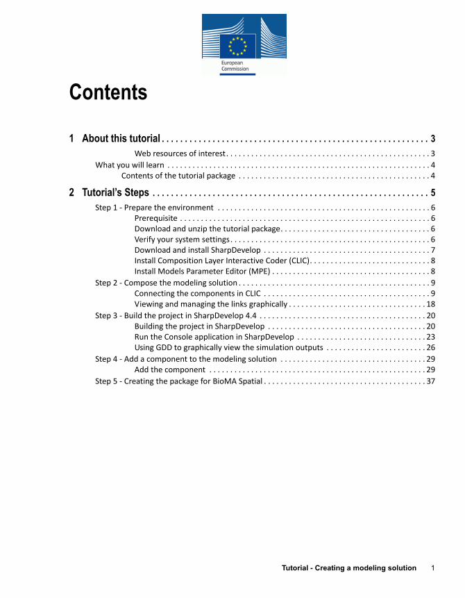
Contents

1 About this tutorial . . . . . . . . . . . . . . . . . . . . . . . . . . . . . . . . . . . . . . . . . . . . . . . . . . . . . . . . . . 3Web resources of interest. . . . . . . . . . . . . . . . . . . . . . . . . . . . . . . . . . . . . . . . . . . . . . . . . 3

What you will learn . . . . . . . . . . . . . . . . . . . . . . . . . . . . . . . . . . . . . . . . . . . . . . . . . . . . . . . . . . . . . . . 4Contents of the tutorial package . . . . . . . . . . . . . . . . . . . . . . . . . . . . . . . . . . . . . . . . . . . . . . 4

2 Tutorial’s Steps . . . . . . . . . . . . . . . . . . . . . . . . . . . . . . . . . . . . . . . . . . . . . . . . . . . . . . . . . . . . 5Step 1 ‐ Prepare the environment . . . . . . . . . . . . . . . . . . . . . . . . . . . . . . . . . . . . . . . . . . . . . . . . . . . 6

Prerequisite . . . . . . . . . . . . . . . . . . . . . . . . . . . . . . . . . . . . . . . . . . . . . . . . . . . . . . . . . . . . 6Download and unzip the tutorial package. . . . . . . . . . . . . . . . . . . . . . . . . . . . . . . . . . . . 6Verify your system settings. . . . . . . . . . . . . . . . . . . . . . . . . . . . . . . . . . . . . . . . . . . . . . . . 6Download and install SharpDevelop . . . . . . . . . . . . . . . . . . . . . . . . . . . . . . . . . . . . . . . . 7Install Composition Layer Interactive Coder (CLIC). . . . . . . . . . . . . . . . . . . . . . . . . . . . . 8Install Models Parameter Editor (MPE) . . . . . . . . . . . . . . . . . . . . . . . . . . . . . . . . . . . . . . 8

Step 2 ‐ Compose the modeling solution . . . . . . . . . . . . . . . . . . . . . . . . . . . . . . . . . . . . . . . . . . . . . . 9Connecting the components in CLIC . . . . . . . . . . . . . . . . . . . . . . . . . . . . . . . . . . . . . . . . 9Viewing and managing the links graphically . . . . . . . . . . . . . . . . . . . . . . . . . . . . . . . . . 18

Step 3 ‐ Build the project in SharpDevelop 4.4 . . . . . . . . . . . . . . . . . . . . . . . . . . . . . . . . . . . . . . . . 20Building the project in SharpDevelop . . . . . . . . . . . . . . . . . . . . . . . . . . . . . . . . . . . . . . 20Run the Console application in SharpDevelop . . . . . . . . . . . . . . . . . . . . . . . . . . . . . . . 23Using GDD to graphically view the simulation outputs . . . . . . . . . . . . . . . . . . . . . . . . 26

Step 4 ‐ Add a component to the modeling solution . . . . . . . . . . . . . . . . . . . . . . . . . . . . . . . . . . . 29Add the component . . . . . . . . . . . . . . . . . . . . . . . . . . . . . . . . . . . . . . . . . . . . . . . . . . . . 29

Step 5 ‐ Creating the package for BioMA Spatial . . . . . . . . . . . . . . . . . . . . . . . . . . . . . . . . . . . . . . . 37

CONTENTS



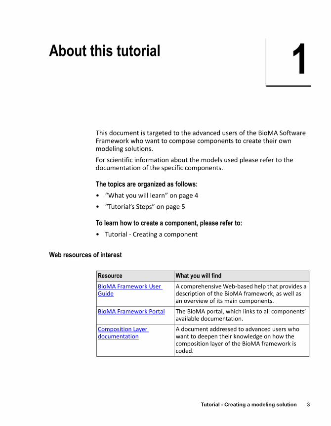
1About this tutorial

This document is targeted to the advanced users of the BioMA Software Framework who want to compose components to create their own modeling solutions.

For scientific information about the models used please refer to the documentation of the specific components.

The topics are organized as follows:

• “What you will learn” on page 4

• “Tutorial’s Steps” on page 5

To learn how to create a component, please refer to:

• Tutorial ‐ Creating a component

Web resources of interest

Resource What you will find

BioMA Framework User Guide

A comprehensive Web‐based help that provides a description of the BioMA framework, as well as an overview of its main components.

BioMA Framework Portal The BioMA portal, which links to all components’ available documentation.

Composition Layer documentation

A document addressed to advanced users who want to deepen their knowledge on how the composition layer of the BioMA framework is coded.

http://bioma.jrc.ec.europa.eu/bioma/help/

http://bioma.jrc.ec.europa.eu/

1 – ABOUT THIS TUTORIAL


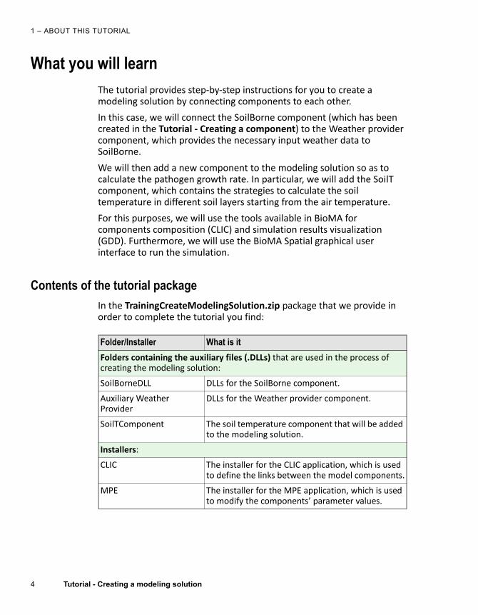
What you will learnThe tutorial provides step‐by‐step instructions for you to create a modeling solution by connecting components to each other.

In this case, we will connect the SoilBorne component (which has been created in the Tutorial ‐ Creating a component) to the Weather provider component, which provides the necessary input weather data to SoilBorne.

We will then add a new component to the modeling solution so as to calculate the pathogen growth rate. In particular, we will add the SoilT component, which contains the strategies to calculate the soil temperature in different soil layers starting from the air temperature.

For this purposes, we will use the tools available in BioMA for components composition (CLIC) and simulation results visualization (GDD). Furthermore, we will use the BioMA Spatial graphical user interface to run the simulation.

Contents of the tutorial packageIn the TrainingCreateModelingSolution.zip package that we provide in order to complete the tutorial you find:

Folder/Installer What is it

Folders containing the auxiliary files (.DLLs) that are used in the process of creating the modeling solution:

SoilBorneDLL DLLs for the SoilBorne component.

Auxiliary Weather Provider

DLLs for the Weather provider component.

SoilTComponent The soil temperature component that will be added to the modeling solution.

Installers:

CLIC The installer for the CLIC application, which is used to define the links between the model components.

MPE The installer for the MPE application, which is used to modify the components’ parameter values.


2Tutorial’s Steps

The steps are organized as follows:

• “Step 1 ‐ Prepare the environment” on page 6

• “Step 2 ‐ Compose the modeling solution” on page 9

• “Step 3 ‐ Build the project in SharpDevelop 4.4” on page 20

• “Step 4 ‐ Add a component to the modeling solution” on page 29

• “Step 5 ‐ Creating the package for BioMA Spatial” on page 37

See also:

• “What you will learn” on page 4

• “Contents of the tutorial package” on page 4

2 – TUTORIAL’S STEPS


Step 1 - Prepare the environmentThis step involves:

• “Download and unzip the tutorial package” on page 6

• “Verify your system settings” on page 6

• “Download and install SharpDevelop” on page 7

• “Install Composition Layer Interactive Coder (CLIC)” on page 8

• “Install Models Parameter Editor (MPE)” on page 8

Prerequisite

You have completed the first Tutorial ‐ Creating a component, which is located in the tutorial package.

Download and unzip the tutorial package

The ZIP package you will download includes all the files you need to complete the tutorial (see “Contents of the tutorial package” on page 4).

To download it:

1 Go to the Agri4Cast Resources Portal (http://agri4cast.jrc.ec.europa.eu/DataPortal/Index.aspx?o=s). Do the following:

a. If you are not registered yet, click Register at the top‐right, then follow the instructions to register.

b. In the Create Bioma Modelling Solution area, click the Download Resources button and download the TrainingCreateModelingSolution.zip file.

2 Unzip the TrainingCreateModelingSolution.zip package we have provided in a folder at your choice in your PC.

Verify your system settings

In order to complete the tutorial, you must have:

• Windows PC (at least 2/3 GB of RAM)

• Administrative rights on the machine

• Microsoft .NET 3.5 (or above) installed

http://agri4cast.jrc.ec.europa.eu/DataPortal/Index.aspx?o=s

http://agri4cast.jrc.ec.europa.eu/DataPortal/Index.aspx?o=s


STEP 1 - PREPARE THE ENVIRONMENT

• A developer IDE (Integrated Developer Environment) installed. This can either be:

‐ Visual Studio 2008 or later versions, or

‐ SharpDevelop 4.4 (free and open source, downloadable from www.icsharpcode.net. See below for instructions.)

• Drivers to use a SQL Server Compact Edition database. You can download the drivers here: http://www.microsoft.com/en‐us/download/details.aspx?displaylang=en&id=5783

• In the settings of the PC, the dot ('.') must be set as the decimal separator. To check this setting:

‐ Access the Windows Control Panel (click the Start button, then select Control Panel > Clock, Language, and Region > Region and Language).

‐ In the Region and Language window, click Additional settings.

‐ Be sure that the Decimal symbol is set to “point” (.).

Download and install SharpDevelop

SharpDevelop is the free and open‐source IDE (Integrated Developer Environment) that allows writing applications in languages including C#, VB.NET and Boo projects on Microsoft's .NET platform.

To install SharpDevelop:

1 Download the Version 4.4 here: www.icsharpcode.net

This tutorial has been prepared using SharpDevelop 4.4. We cannot guarantee it will work with a later version even if it is very likely.

2 Follow the instructions to install the application. As a result, a shortcut will be created on the desktop.

3 Double‐click the shortcut to launch the application.

Note:

If you have Microsoft Visual Studio 2008 or above installed in your PC, you can use it rather than using SharpDevelop. The procedure for creating and editing a project is very similar.

www.icsharpcode.net

http://www.microsoft.com/en-us/download/details.aspx?displaylang=en&id=5783

http://www.microsoft.com/en-us/download/details.aspx?displaylang=en&id=5783

http://www.icsharpcode.net/OpenSource/SD/Download/#SharpDevelop4x



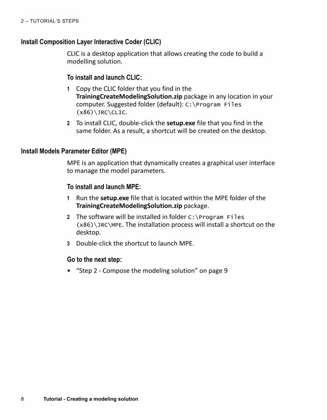
Install Composition Layer Interactive Coder (CLIC)

CLIC is a desktop application that allows creating the code to build a modelling solution.

To install and launch CLIC:

1 Copy the CLIC folder that you find in the TrainingCreateModelingSolution.zip package in any location in your computer. Suggested folder (default): C:\Program Files (x86)\JRC\CLIC.

2 To install CLIC, double‐click the setup.exe file that you find in the same folder. As a result, a shortcut will be created on the desktop.

Install Models Parameter Editor (MPE)

MPE is an application that dynamically creates a graphical user interface to manage the model parameters.

To install and launch MPE:

1 Run the setup.exe file that is located within the MPE folder of the TrainingCreateModelingSolution.zip package.

2 The software will be installed in folder C:\Program Files (x86)\JRC\MPE. The installation process will install a shortcut on the desktop.

3 Double‐click the shortcut to launch MPE.

Go to the next step:

• “Step 2 ‐ Compose the modeling solution” on page 9


STEP 2 - COMPOSE THE MODELING SOLUTION

Step 2 - Compose the modeling solution

Before starting this step

We assume that you have completed the Tutorial ‐ Creating a component located in the package we have provided (see “Download and unzip the tutorial package” on page 6). The tutorial guides you through the steps of creating the new component MY.EXAMPLE.SoilBorne containing a strategy with the aim to simulate the soil borne fungal pathogens growth. This is actually the output of the first tutorial.

Goal of this step

In this step we will build the modeling solution by connecting two model components to each other and by defining their order of execution in the model.

At the end, the modelling solution will contain two components:

• SoilBorne pathogen component

• WeatherProvider component

The aim of this modeling solution is to calculate the pathogen growth rate by using the air temperature.

See:

• “Connecting the components in CLIC” on page 9

• “Viewing and managing the links graphically” on page 18

Connecting the components in CLIC

To launch CLIC and build the model:

1 Launch CLIC by double‐clicking the shortcut that was created during the installation process (see “Install Composition Layer Interactive Coder (CLIC)” on page 8).

2 Note that two windows are displayed, the CLIC start window and a Visio window, which opens on the back:

Note:

For further information on how to use CLIC, please refer to the embedded help online, which you can reach by clicking the Help button at the bottom-right of the application’s window.



The window on the back provides a graphical view of the components’ links once these have been connected. (See “Viewing and managing the links graphically” on page 18).

3 Click the Create/modify a model runner button.

4 In the Load existing components window that is displayed, click the Load libraries button.

5 Browse to the [TutorialInstallationFolder]/SoilBorneDLL folder of the tutorial package, select all the DLLs and click Open.

As a result, the DLLs will be listed in the Loaded libraries upper pane.

6 Click the Load libraries button, again.



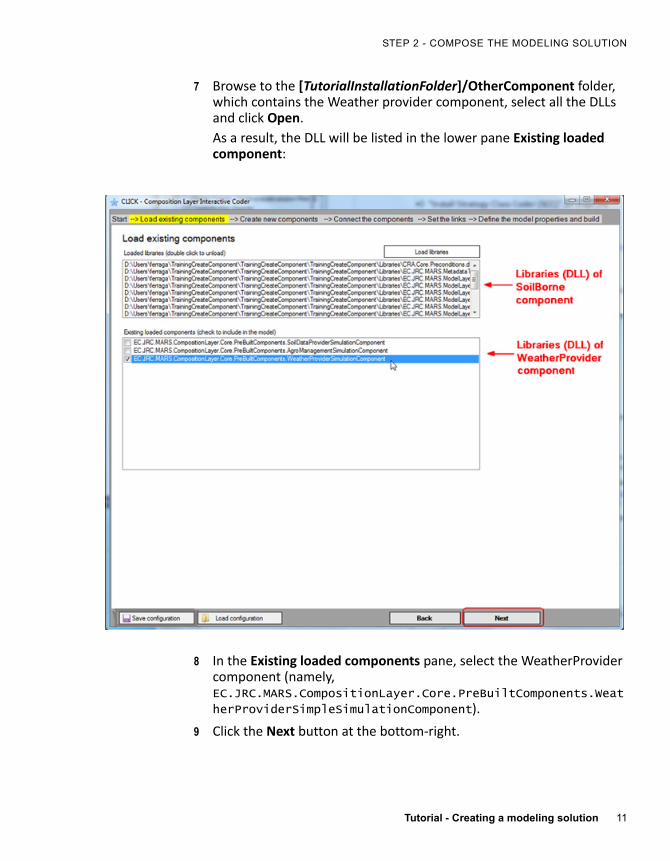
7 Browse to the [TutorialInstallationFolder]/OtherComponent folder, which contains the Weather provider component, select all the DLLs and click Open.

As a result, the DLL will be listed in the lower pane Existing loaded component:

8 In the Existing loaded components pane, select the WeatherProvider component (namely, EC.JRC.MARS.CompositionLayer.Core.PreBuiltComponents.Weat

herProviderSimpleSimulationComponent).

9 Click the Next button at the bottom‐right.



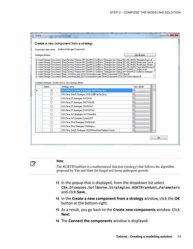
10 In the Create new components window that is displayed, enter a name for the component, for example, SoilBornePathogenComponent:

11 Click the Create component from strategy button.

12 In the window that is displayed, select from the Available strategies list the RGRTRYanHunt strategy, as shown below:



13 In the popup that is displayed, from the dropdown list select CRA.Diseases.SoilBorne.Strategies.RGRTRYanHunt_Parameters and click Save.

14 In the Create a new component from a strategy window, click the OK button at the bottom‐right.

15 As a result, you go back to the Create new components window. Click Next.

16 The Connect the components window is displayed:

Note:

The RGRTRYanHunt is a mathematical function (strategy) that follows the algorithm proposed by Yan and Hunt for fungal soil borne pathogens growth.



17 Under Specify connections, select from the dropdown lists the following (as shown above):

‐ Source component: WeatherProviderSimulationComponent

‐ Destination component: SoilBornePathogenComponent

18 Click the Next button at the bottom‐right. The Set the links between components window is displayed:

19 Click the Edit links button.

20 In the Set the links between the domain classes of the components window that is displayed, select from the dropdown lists the following:

‐ Source domain class: Grid_weather

‐ Destination domain class: Exogenous

21 Click the Edit properties links button:



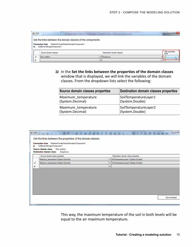
22 In the Set the links between the properties of the domain classes window that is displayed, we will link the variables of the domain classes. From the dropdown lists select the following:

This way, the maximum temperature of the soil in both levels will be equal to the air maximum temperature.

Source domain classes properties Destination domain classes properties

Maximum_temperature (System.Decimal)

SoilTemperatureLayer1 (System.Double)

Maximum_temperature (System.Decimal)

SoilTemperatureLayer2 (System.Double)



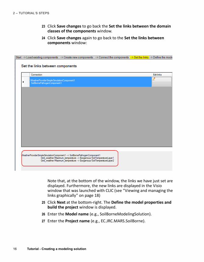
23 Click Save changes to go back the Set the links between the domain classes of the components window.

24 Click Save changes again to go back to the Set the links between components window:

Note that, at the bottom of the window, the links we have just set are displayed. Furthermore, the new links are displayed in the Visio window that was launched with CLIC (see “Viewing and managing the links graphically” on page 18)

25 Click Next at the bottom‐right. The Define the model properties and build the project window is displayed.

26 Enter the Model name (e.g., SoilBorneModelingSolution).

27 Enter the Project name (e.g., EC.JRC.MARS.SoilBorne).



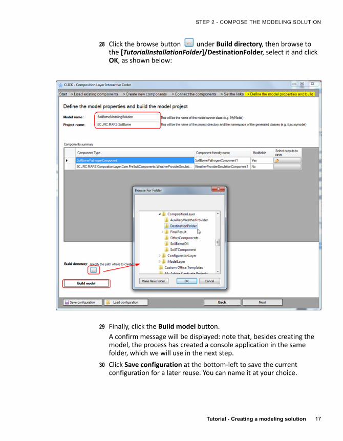
28 Click the browse button under Build directory, then browse to the [TutorialInstallationFolder]/DestinationFolder, select it and click OK, as shown below:

29 Finally, click the Build model button.

A confirm message will be displayed: note that, besides creating the model, the process has created a console application in the same folder, which we will use in the next step.

30 Click Save configuration at the bottom‐left to save the current configuration for a later reuse. You can name it at your choice.



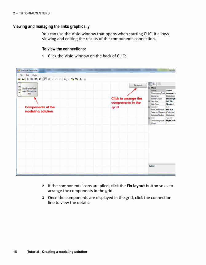
Viewing and managing the links graphically

You can use the Visio window that opens when starting CLIC. It allows viewing and editing the results of the components connection.

To view the connections:

1 Click the Visio window on the back of CLIC:

2 If the components icons are piled, click the Fix layout button so as to arrange the components in the grid.

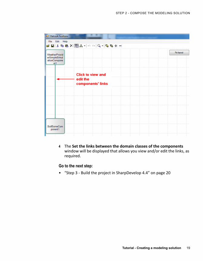
3 Once the components are displayed in the grid, click the connection line to view the details:



4 The Set the links between the domain classes of the components window will be displayed that allows you view and/or edit the links, as required.


• “Step 3 ‐ Build the project in SharpDevelop 4.4” on page 20



Step 3 - Build the project in SharpDevelop 4.4In this step, we will complete two tasks:

• Build the project that was created in the previous step and add the console application. (See “Building the project in SharpDevelop” on page 20)

• Run the console application and launch Graphic Data Display (GDD). (See “Run the Console application in SharpDevelop” on page 23)

• Use GDD to graphically view the simulation outputs (see “Using GDD to graphically view the simulation outputs” on page 26).

Building the project in SharpDevelop

To build the SoilBorne project:

1 Launch SharpDevelop by double‐clicking the shortcut that was created on your desktop through the installation process.

2 From the SharpDevelop menu bar, select File > Open > Project/Solution.

3 Browse to select the [TutorialInstallationFolder]/Destination Folder /CompositionLayerModelingSolution folder, then select the EC.JRC.MARS.SoilBorne.csproj you have created in the previous step and click Open.

4 In the Projects pane of SharpDevelop, right‐click the project and select Build:


STEP 3 - BUILD THE PROJECT IN SHARPDEVELOP 4.4

I

Wait for the procedure to complete. The project should build successfully.

To add the ConsoleApplication and build the project:

Now, we will add to the SharpDevelop solution the ConsoleApplication that was created via CLIC in Step 2:

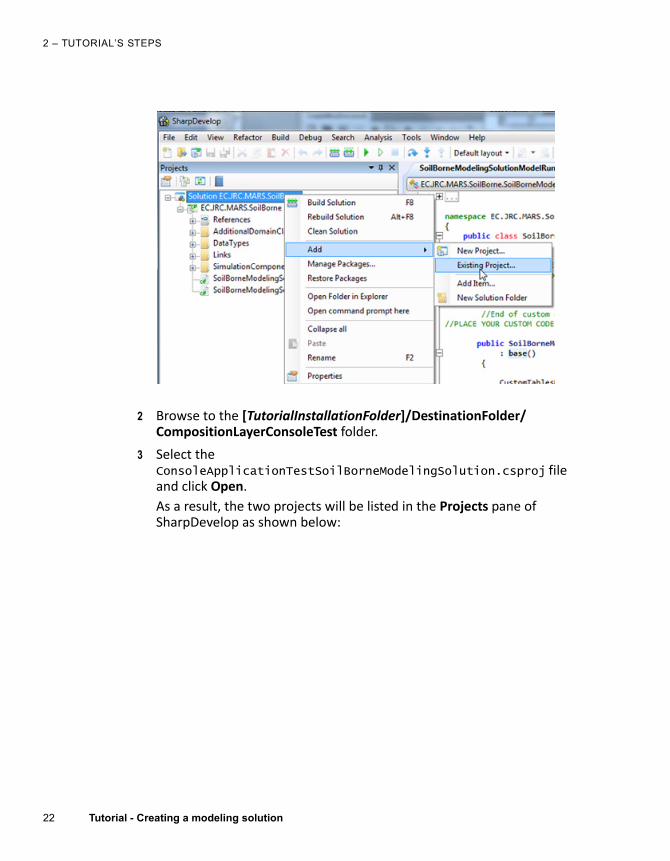
1 in the Project pane of SharpDevelop, right‐click the main solution (as shown below) and select Add > Existing project:



2 Browse to the [TutorialInstallationFolder]/DestinationFolder/CompositionLayerConsoleTest folder.

3 Select the ConsoleApplicationTestSoilBorneModelingSolution.csproj file and click Open.

As a result, the two projects will be listed in the Projects pane of SharpDevelop as shown below:



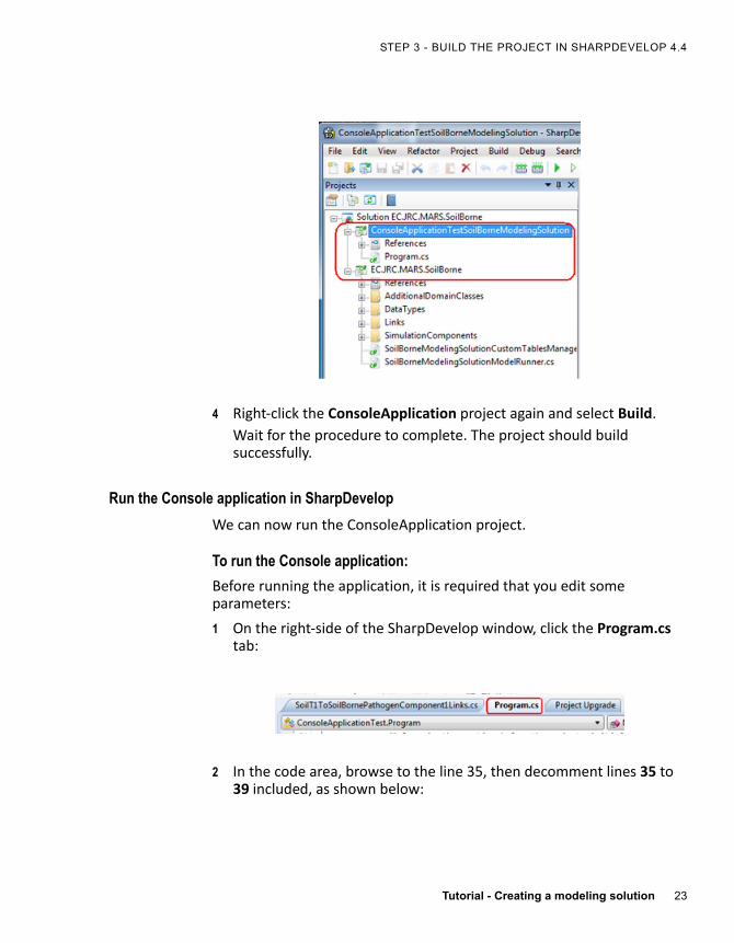
4 Right‐click the ConsoleApplication project again and select Build.

Wait for the procedure to complete. The project should build successfully.

Run the Console application in SharpDevelop

We can now run the ConsoleApplication project.

To run the Console application:

Before running the application, it is required that you edit some parameters:

1 On the right‐side of the SharpDevelop window, click the Program.cs tab:

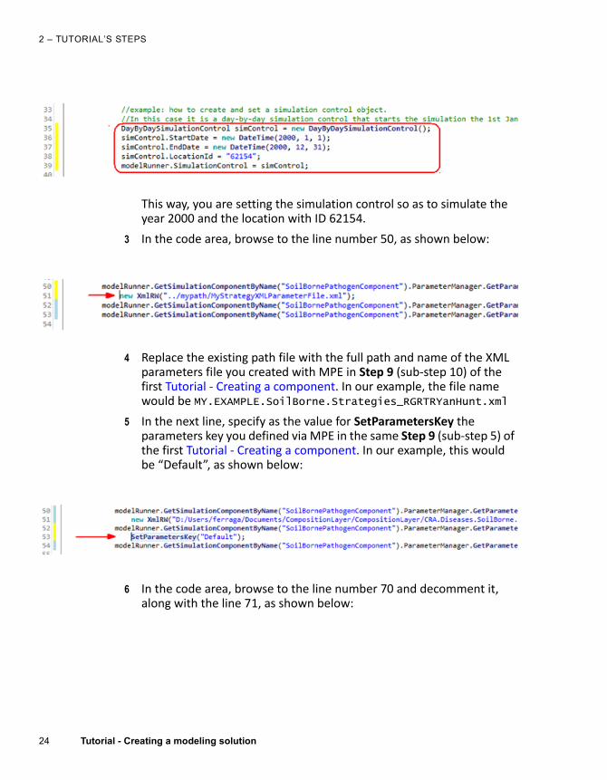
2 In the code area, browse to the line 35, then decomment lines 35 to 39 included, as shown below:



This way, you are setting the simulation control so as to simulate the year 2000 and the location with ID 62154.

3 In the code area, browse to the line number 50, as shown below:

4 Replace the existing path file with the full path and name of the XML parameters file you created with MPE in Step 9 (sub‐step 10) of the first Tutorial ‐ Creating a component. In our example, the file name would be MY.EXAMPLE.SoilBorne.Strategies_RGRTRYanHunt.xml

5 In the next line, specify as the value for SetParametersKey the parameters key you defined via MPE in the same Step 9 (sub‐step 5) of the first Tutorial ‐ Creating a component. In our example, this would be “Default”, as shown below:

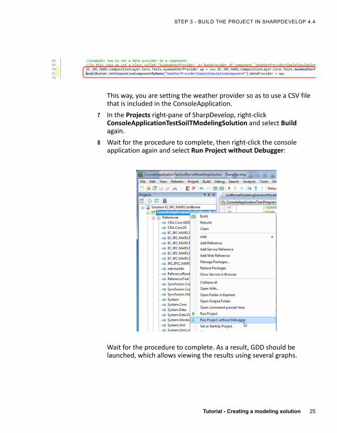
6 In the code area, browse to the line number 70 and decomment it, along with the line 71, as shown below:



This way, you are setting the weather provider so as to use a CSV file that is included in the ConsoleApplication.

7 In the Projects right‐pane of SharpDevelop, right‐click ConsoleApplicationTestSoilTModelingSolution and select Build again.

8 Wait for the procedure to complete, then right‐click the console application again and select Run Project without Debugger:

Wait for the procedure to complete. As a result, GDD should be launched, which allows viewing the results using several graphs.



Using GDD to graphically view the simulation outputs

GDD, that opens after running the console application, allows viewing the model simulation outputs, both in graphical and tabular forms.

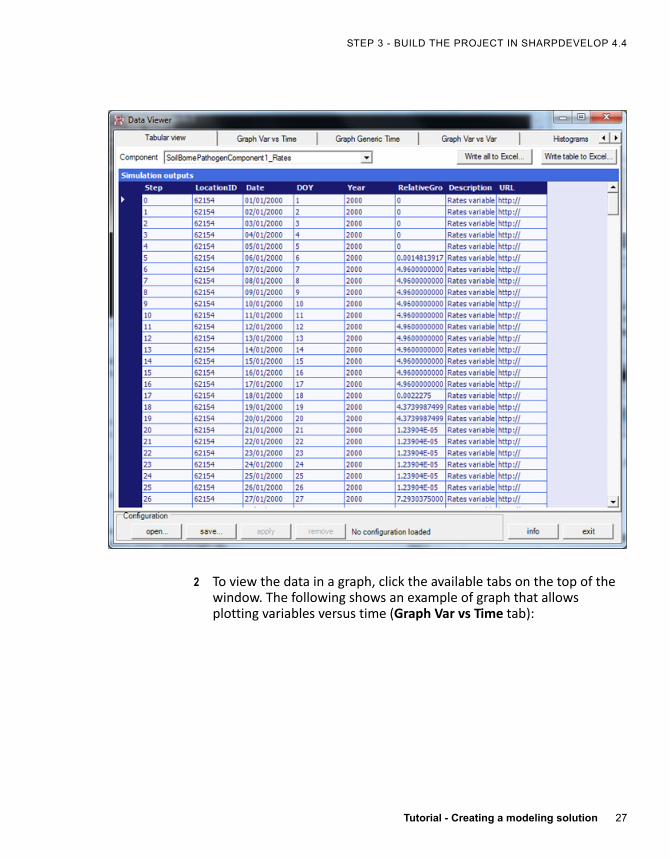
1 In the GDD main window, from the Component dropdown list at the top, select an item. For the sake of this tutorial, we will select SoilBornePathogenComponent_Rates:

As a result the Simulation outputs’ data will be displayed in the window:



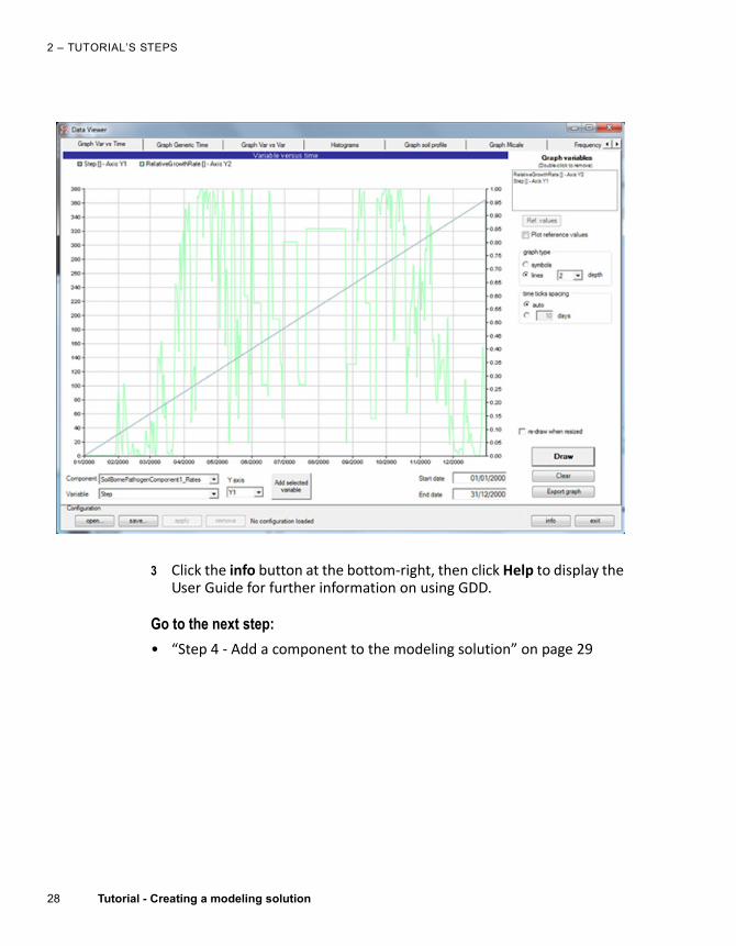
2 To view the data in a graph, click the available tabs on the top of the window. The following shows an example of graph that allows plotting variables versus time (Graph Var vs Time tab):



3 Click the info button at the bottom‐right, then click Help to display the User Guide for further information on using GDD.


• “Step 4 ‐ Add a component to the modeling solution” on page 29


STEP 4 - ADD A COMPONENT TO THE MODELING SOLUTION

Step 4 - Add a component to the modeling solutionIn this step, we will add a new component (SoilT) to the new modelling solution, which, as a result, will contain three components:

• SoilBorne pathogen component

• WeatherProvider component

• SoilT component (which is provided in the tutorial package within the folder [TutorialInstallationFolder]/SoilTComponent)

Modeling solution purpose - Why SoilT must be added

We want to calculate the pathogen growth rate by using the soil temperature rather than the air temperature.

For this purpose, we must use the SoilT component, which contains the strategies to calculate the soil temperature in different soil layers starting from the air temperature.

The inputs needed by the SoilT component are:

• Minimum air temperature

• Maximum air temperature

• Solar radiation

We will then set the links between the WeatherComponent and the SoilT components, as well as, between the SoilT and the SoilBorne pathogen components.

Add the component

To add the SoilT component in CLIC:

1 Go back to CLIC. (If you closed CLIC without saving your configuration, you must repeat “Step 2 ‐ Compose the modeling solution” on page 9).

2 Click the Load configuration button at the bottom‐left, then browse to select the configuration you saved in Step 2.

3 In the Load existing components window that is displayed, click Load libraries, then browse to the [TutorialInstallationFolder]/SoilTComponent folder of the tutorial package, select all DLLs, and click Open. The libraries will be added to the Loaded libraries upper pane.



4 In the Existing loaded components lower pane, select the SoilT component (namely, EC.JRC.MARS.SoilTComponent.SoilT).

5 Click the Next button at the bottom‐right.

6 In the Create new components window that is displayed, click Next. The Connect the components window is displayed.

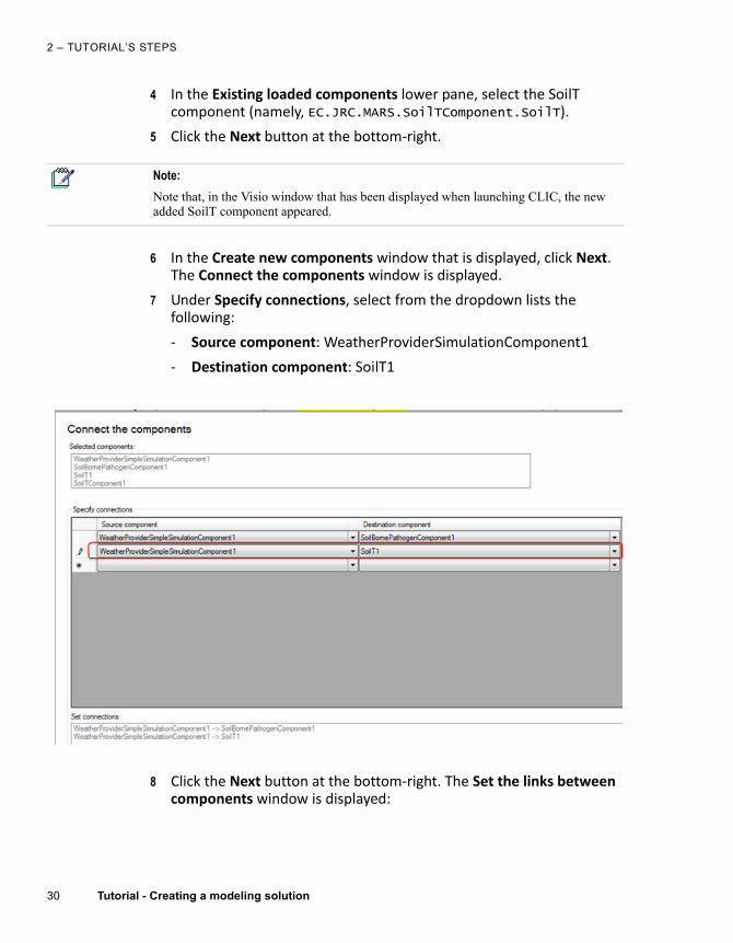
7 Under Specify connections, select from the dropdown lists the following:

‐ Source component: WeatherProviderSimulationComponent1

‐ Destination component: SoilT1

8 Click the Next button at the bottom‐right. The Set the links between components window is displayed:

Note:

Note that, in the Visio window that has been displayed when launching CLIC, the new added SoilT component appeared.



9 Select the Connection you just created (as shown above) and click the Edit links button.

10 In the Set the links between the domain classes of the components window that is displayed, select from the dropdown lists the following:

‐ Source domain class: Grid_weather

‐ Destination domain class: SoilTemperatureExogenous

as shown below:

11 Click the Edit properties links button.

12 The window Set the links between the properties of the domain classes is displayed. We want to set the links in both levels so that the soil temperature is equal to the max air temperature.

For this purpose, set the following values:



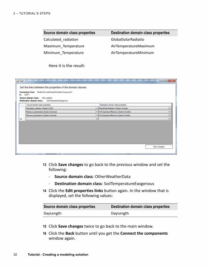
Here it is the result:

13 Click Save changes to go back to the previous window and set the following:

‐ Source domain class: OtherWeatherData

‐ Destination domain class: SoilTemperatureExogenous

14 Click the Edit properties links button again. In the window that is displayed, set the following values:

15 Click Save changes twice to go back to the main window.

16 Click the Back button until you get the Connect the components window again.

Source domain class properties Destination domain class properties

Calculated_radiation GlobalSolarRadiatio

Maximum_Temperature AirTemperatureMaximum

Minimum_Temperature AirTemperatureMinimum


DayLength DayLength



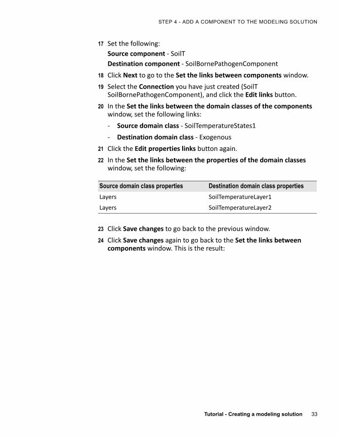
17 Set the following:

Source component ‐ SoilT

Destination component ‐ SoilBornePathogenComponent

18 Click Next to go to the Set the links between components window.

19 Select the Connection you have just created (SoilT SoilBornePathogenComponent), and click the Edit links button.

20 In the Set the links between the domain classes of the components window, set the following links:

‐ Source domain class ‐ SoilTemperatureStates1

‐ Destination domain class ‐ Exogenous

21 Click the Edit properties links button again.

22 In the Set the links between the properties of the domain classes window, set the following:

23 Click Save changes to go back to the previous window.

24 Click Save changes again to go back to the Set the links between components window. This is the result:


Layers SoilTemperatureLayer1

Layers SoilTemperatureLayer2



25 Click Next at the bottom‐right of the window. The Define the model properties and build the project window is displayed.

26 Enter the Model name (e.g., SoilTModelingSolution).

27 Enter the Project name (e.g., EC.JRC.MARS.SoilT).

28 Click the browse button under Build directory.

29 In the Browse For Folder popup that is displayed browse to the [TutorialInstallationFolder] folder, select it, and then click the Make New Folder button.

30 Name the new folder at your choice (e.g., DestinationFolder2), select it, and then click OK.

31 Click Build model.

At this point, all the components have been connected as the Visio window on the back of CLIC will shows (click Fix layout to order the elements on the grid, if needed):



By clicking the arrows that connect the components, the following is displayed, which allows you to view and edit the links between the components’ domain classes:




• “Step 5 ‐ Creating the package for BioMA Spatial” on page 37


STEP 5 - CREATING THE PACKAGE FOR BIOMA SPATIAL

Step 5 - Creating the package for BioMA SpatialIn this step, we will create a package to run the modelling solution in BioMA Spatial.

For this purpose we will add the project that was created via CLIC (see “Step 4 ‐ Add a component to the modeling solution” on page 29) to the Projects pane in SharpDevelop.

To add the project in SharpDevelop:

1 Launch SharpDevelop (which you installed as described in “Download and install SharpDevelop” on page 7).

2 Open the solution you created in “Step 3 ‐ Build the project in SharpDevelop 4.4” on page 20.

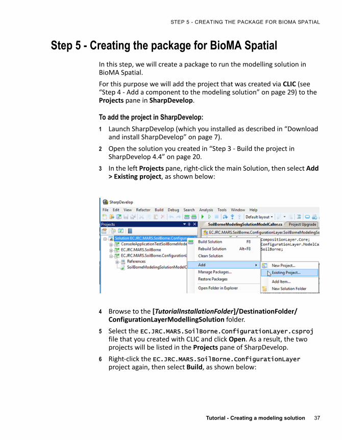
3 In the left Projects pane, right‐click the main Solution, then select Add > Existing project, as shown below:

4 Browse to the [TutorialInstallationFolder]/DestinationFolder/ConfigurationLayerModellingSolution folder.

5 Select the EC.JRC.MARS.SoilBorne.ConfigurationLayer.csproj file that you created with CLIC and click Open. As a result, the two projects will be listed in the Projects pane of SharpDevelop.

6 Right‐click the EC.JRC.MARS.SoilBorne.ConfigurationLayer project again, then select Build, as shown below:



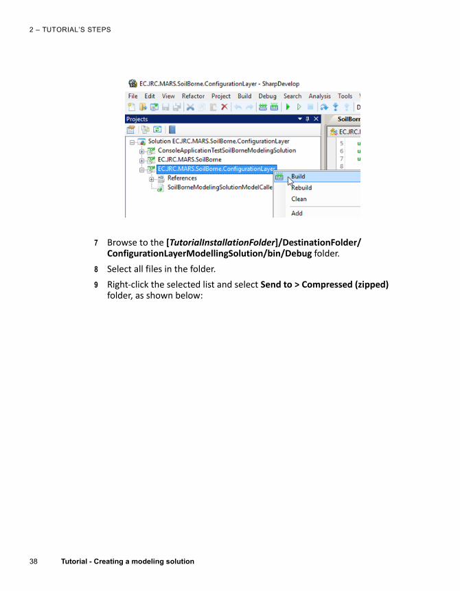
7 Browse to the [TutorialInstallationFolder]/DestinationFolder/ConfigurationLayerModellingSolution/bin/Debug folder.

8 Select all files in the folder.

9 Right‐click the selected list and select Send to > Compressed (zipped) folder, as shown below:


STEP 5 - CREATING THE PACKAGE FOR BIOMA SPATIAL

10 Rename the resulting zipped file by changing the name and the extension from .zip to .bpkg (e.g.: SoilBorne.bpkg).

Now the package is ready and it can be used to run the modelling solution in BioMA Spatial.

For information on how to use BioMA Spatial see the “BioMA Spatial User Guide”:

• Online version: http://bioma.jrc.ec.europa.eu/spatial/Help/index.htm

• PDF version: http://bioma.jrc.ec.europa.eu/documentation/BioMA_Spatial_User_Guide.pdf.

http://bioma.jrc.ec.europa.eu/spatial/Help/index.htm

http://bioma.jrc.ec.europa.eu/documentation/BioMA_Spatial_User_Guide.pdf

http://bioma.jrc.ec.europa.eu/documentation/BioMA_Spatial_User_Guide.pdf

introducing bioma - europabioma.jrc.ec.europa.eu/tutorials/creating_modeling_solution.pdf · 1 –...

Documents