introducing spm® infrastructure - minitab.com · the spm® can be installed on windows 7 and...
TRANSCRIPT

Introducing SPM®
Infrastructure

© 2019 Minitab, LLC. All Rights Reserved.
Minitab®, SPM®, SPM Salford Predictive Modeler®, Salford Predictive Modeler®, Random Forests®, CART®, TreeNet®, MARS®, RuleLearner®, and the Minitab logo are registered trademarks of Minitab, LLC. in the United States and other countries. Additional trademarks of Minitab, LLC. can be found at www.minitab.com. All other marks referenced remain the property of their respective owners.

Salford Predictive Modeler® Introducing SPM® Infrastructure
3
Introducing SPM® Infrastructure
The SPM® application is structured around major predictive analysis scenarios. In general, the workflow
of the application can be described as follows.
Bring data for analysis to the application.
Research the data, if needed.
Configure and build a predictive analytics model.
Review the results of the run. Discover the model that captures valuable insight about the data.
Score the model. For example, you could simulate future events.
Export the model to a format other systems can consume. This could be PMML or executable code in a mainstream or specialized programming language.
Document the analysis.
The nature of predictive analysis methods you use and the nature of the data itself could dictate particular
unique steps in the scenario. Some actions and mechanisms, though, are common. For any analysis you
need to bring the data in and get some understanding of it. When reviewing the results of the modeling
and preparing documentation, you can make use of special features embedded into charts and grids.
While we make sure to offer a display to visualize particular results, there’s always a Summary window
that brings you a standard set of results represented the same familiar way throughout the application.
The SPM® also provides a handy unified way to document the analysis.
This guide discusses common mechanisms available all over the user interface. It augments the
information specific to Analysis Engines (CART®, TreeNet® etc.) provided by other guides.
Installing and Starting SPM®
The SPM® can be installed on Windows 7 and higher versions of Windows. Although application may run
on older versions of the Windows Operating System we strongly recommend that you rely on the latest
version of Windows.
Minimum Windows System Requirements
Operating System Windows 7 SP 1 or later, Windows 8 or 8.1, Windows 10.
RAM 2 GB.
Processor Intel® Pentium® 4 or AMD Athlon™ Dual Core, with SSE2 technology.
Hard Disk Space 2 GB (minimum) free space available.
Screen Resolution 1024 x 768 or higher.
Minimum Linux System Requirements
Operating System Ubuntu 14.04 or 16.04, CentOS 6.9 or 7.5, RHEL 6.9 or 7.5.
RAM 2 GB.
Processor Intel® Pentium® 4 or AMD Athlon™ Dual Core, with SSE2 technology
Hard Disk Space 2 GB (minimum) free space available.
Salford Predictive Modeler® Introducing SPM® Infrastructure
4
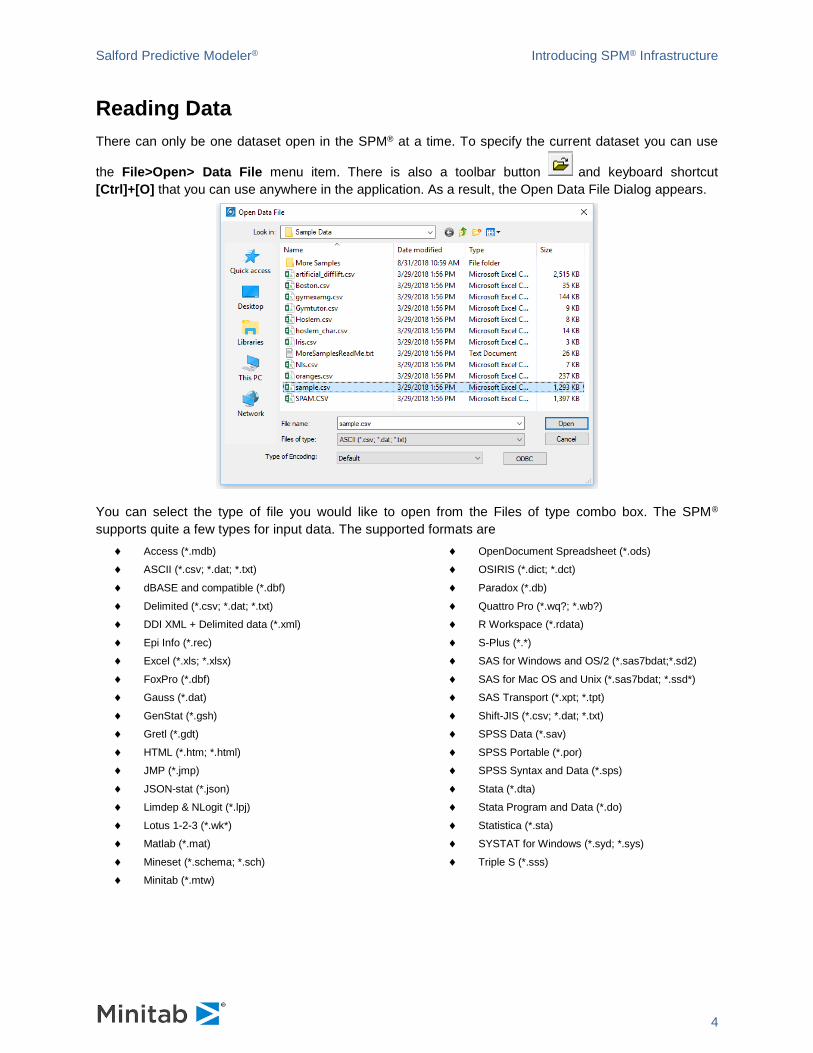
Reading Data
There can only be one dataset open in the SPM® at a time. To specify the current dataset you can use
the File>Open> Data File menu item. There is also a toolbar button and keyboard shortcut
[Ctrl]+[O] that you can use anywhere in the application. As a result, the Open Data File Dialog appears.
You can select the type of file you would like to open from the Files of type combo box. The SPM®
supports quite a few types for input data. The supported formats are
Access (*.mdb)
ASCII (*.csv; *.dat; *.txt)
dBASE and compatible (*.dbf)
Delimited (*.csv; *.dat; *.txt)
DDI XML + Delimited data (*.xml)
Epi Info (*.rec)
Excel (*.xls; *.xlsx)
FoxPro (*.dbf)
Gauss (*.dat)
GenStat (*.gsh)
Gretl (*.gdt)
HTML (*.htm; *.html)
JMP (*.jmp)
JSON-stat (*.json)
Limdep & NLogit (*.lpj)
Lotus 1-2-3 (*.wk*)
Matlab (*.mat)
Mineset (*.schema; *.sch)
Minitab (*.mtw)
OpenDocument Spreadsheet (*.ods)
OSIRIS (*.dict; *.dct)
Paradox (*.db)
Quattro Pro (*.wq?; *.wb?)
R Workspace (*.rdata)
S-Plus (*.*)
SAS for Windows and OS/2 (*.sas7bdat;*.sd2)
SAS for Mac OS and Unix (*.sas7bdat; *.ssd*)
SAS Transport (*.xpt; *.tpt)
Shift-JIS (*.csv; *.dat; *.txt)
SPSS Data (*.sav)
SPSS Portable (*.por)
SPSS Syntax and Data (*.sps)
Stata (*.dta)
Stata Program and Data (*.do)
Statistica (*.sta)
SYSTAT for Windows (*.syd; *.sys)
Triple S (*.sss)
Salford Predictive Modeler® Introducing SPM® Infrastructure
5
For any of the formats you can specify character encoding using the Type of Encoding combo box.
Default will let the data reading layer to determine the encoding. The supported encodings are
US-ASCII
SHIFT-JIS
SHIFT_JIS
CP932
EUC-JP
ISO-2022-JP
ISO-2022-JP-1
ISO-2022-JP-2
UTF-8
UTF-16
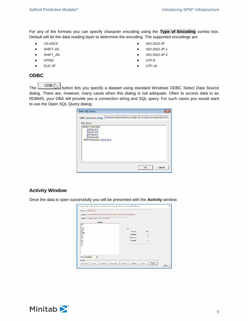
ODBC
The button lets you specify a dataset using standard Windows ODBC Select Data Source
dialog. There are, however, many cases when this dialog is not adequate. Often to access data in an
RDBMS, your DBA will provide you a connection string and SQL query. For such cases you would want
to use the Open SQL Query dialog:
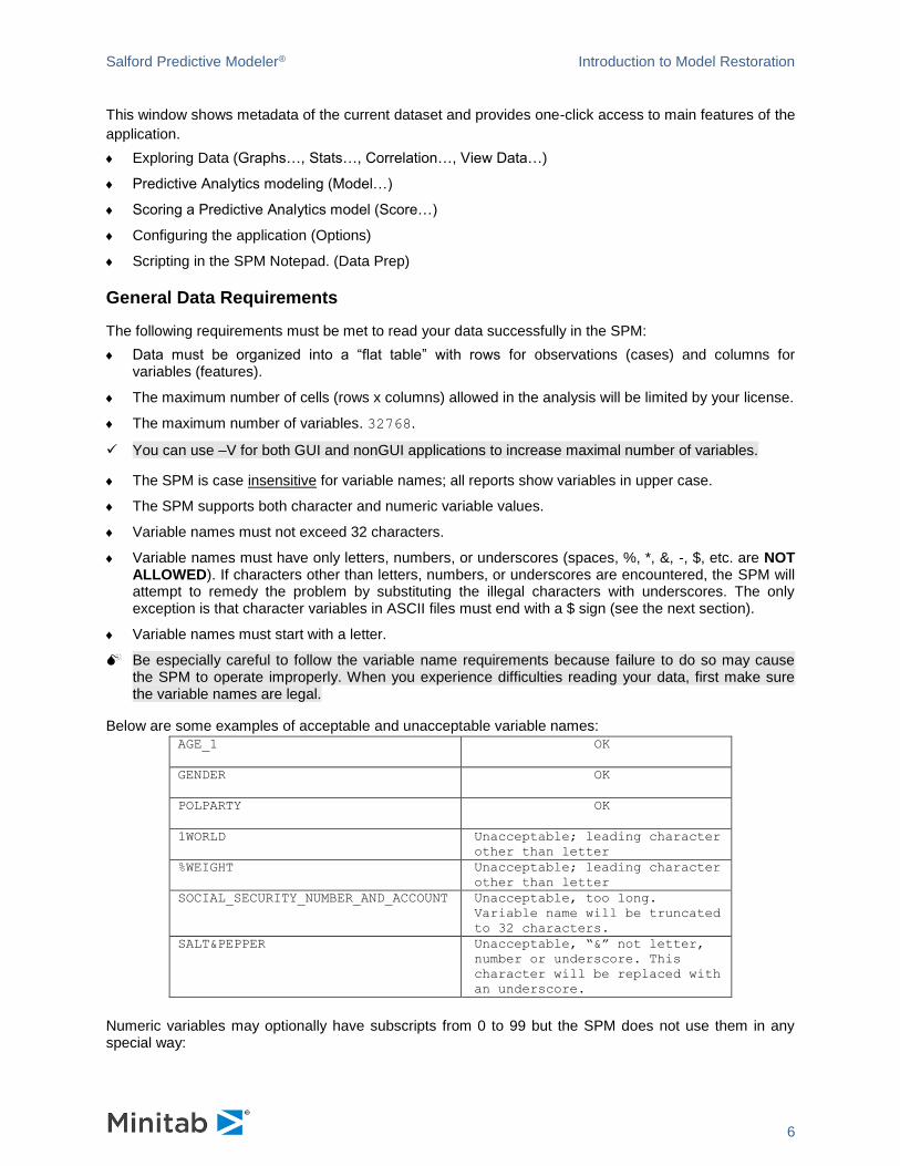
Activity Window
Once the data is open successfully you will be presented with the Activity window.
Salford Predictive Modeler® Introduction to Model Restoration
6
This window shows metadata of the current dataset and provides one-click access to main features of the
application.
Exploring Data (Graphs…, Stats…, Correlation…, View Data…)
Predictive Analytics modeling (Model…)
Scoring a Predictive Analytics model (Score…)
Configuring the application (Options)
Scripting in the SPM Notepad. (Data Prep)
General Data Requirements
The following requirements must be met to read your data successfully in the SPM:
Data must be organized into a “flat table” with rows for observations (cases) and columns for variables (features).
The maximum number of cells (rows x columns) allowed in the analysis will be limited by your license.
The maximum number of variables. 32768.
✓ You can use –V for both GUI and nonGUI applications to increase maximal number of variables.
The SPM is case insensitive for variable names; all reports show variables in upper case.
The SPM supports both character and numeric variable values.
Variable names must not exceed 32 characters.
Variable names must have only letters, numbers, or underscores (spaces, %, *, &, -, $, etc. are NOT ALLOWED). If characters other than letters, numbers, or underscores are encountered, the SPM will attempt to remedy the problem by substituting the illegal characters with underscores. The only exception is that character variables in ASCII files must end with a $ sign (see the next section).
Variable names must start with a letter.
Be especially careful to follow the variable name requirements because failure to do so may cause the SPM to operate improperly. When you experience difficulties reading your data, first make sure the variable names are legal.
Below are some examples of acceptable and unacceptable variable names: AGE_1 OK
GENDER OK
POLPARTY OK
1WORLD Unacceptable; leading character
other than letter
%WEIGHT Unacceptable; leading character
other than letter
SOCIAL_SECURITY_NUMBER_AND_ACCOUNT Unacceptable, too long.
Variable name will be truncated
to 32 characters.
SALT&PEPPER Unacceptable, “&” not letter,
number or underscore. This
character will be replaced with
an underscore.
Numeric variables may optionally have subscripts from 0 to 99 but the SPM does not use them in any special way:

Salford Predictive Modeler® Introduction to Model Restoration
7
CREDIT(1) OK
SCORE(99) OK
ARRAY(0) OK
ARRAY(100) Unacceptable; parenthesis will be
replaced with underscore.
(1) Unacceptable; parenthesis will be
replaced with underscore.
x() Unacceptable; parenthesis will be
replaced with underscore.
x(1)(2) Unacceptable; parenthesis will be
replaced with underscore.
When using raw ASCII text does not check for, or alter, duplicate variable names in your datasets. SPM does not check for, or alter, duplicate variable names in your dataset.
Comments on Specific Data Formats
Many data analysts already have preferred database formats and use widely known systems such as
SAS® to manage and store data. If you use a format we support, then reading in data is as simple as
opening the file. The Excel file format is the most challenging because Excel allows you to enter data and
column headers in a free format that may conflict with most data analysis conventions. To successfully
import Excel spreadsheets, be sure to follow the variable (column header) naming conventions below.
If you prefer to manage your data as plain ASCII files you will need to follow the simple rules we list below to ensure successful data import.
Reading ASCII Files
The SPM has the built-in capability to read various forms of delimited raw ASCII text files. Optionally,
spaces, tabs or semicolons instead of commas can separate the data, although a single delimiter must be
used throughout the text data file.
ASCII files must have one observation per line. The first line shall contain variable names (see the
necessary requirements for variable names in the previous section). As previously noted, variable names
and values are usually separated using the comma (“,”) character. For example:
DPV,PRED1,CHAR2$,PRED3,CHAR4$,PRED5,PRED6,PRED7,PRED8,PRED9,PRED10,IDVAR
0,-2.32,"MALE",-3.05,"B",-0.0039,-0.32,0.17,0.051,-0.70,-0.0039,1
0,-2.32,"FEMALE",-2.97,"O",0.94,1.59,-0.80,-1.86,-0.68,0.940687,2
1,-2.31,"MALE",-2.96,"H",0.05398,0.875059,-1.0656,0.102,0.35215,0.0539858,3
1,-2.28,"FEMALE",-2.9567,"O",-1.27,0.83,0.200,0.0645709,1.62013,-1.2781,4
The SPM uses the following assumptions to distinguish numeric variables from character variables in
ASCII files:
When a variable name ends with "$," or if the data value is surrounded by quotes (either ' or ") on the first record, or both, it is processed as a character variable. In this case, a $ will be added to the variable name if needed.
If a variable name does NOT end with "$," and if the first record data value is NOT surrounded by quotes, the variable is treated as numeric.
✓ It is safest to use "$" to indicate character fields. Quoting character fields is necessary if "$" is not used at the end of the variable name or if the character data string contains commas (which would otherwise be construed as field separators).

Salford Predictive Modeler® Introduction to Model Restoration
8
✓ Character variables are automatically treated as discrete (categorical). Logically, this is because only numeric values can be continuous in nature.
When a variable name does not end with a $ sign, the variable is treated as numeric. In this case, if a character value is encountered it is automatically replaced by a missing value.
Missing Value Indicators
When a variable contains missing values, SPM® uses the following missing values indicator conventions.
Numeric
Either a dot or nothing at all (e.g., comma followed by comma). In the following example records, the third
variable is missing.
DPV$,PRED1,PRED2,PRED3
"male",1,,5
"female",2,.,6

Salford Predictive Modeler® Introduction to Model Restoration
9
Character
Either an empty quote string (quote marks with nothing in between), or nothing at all (e.g., comma
followed by comma). In the following example records, the first and fourth variables are missing.
DPV$,CHAR1$,PRED2, CHAR3$,PRED4
"male","",1,3.5,,"Calif"
"female",,2,4,'',"Illinois"
Reading Excel Files
We have found that many users like to use Excel files. However, care must be exercised when doing this.
Make sure that the following requirements are met:
The Excel file must contain only a single data sheet; no charts, macros or other items are allowed.
Currently, the Excel data format limits the number of variables to 256 and the number of records to 65535.
The Excel file must not be currently open in another application (e.g. Microsoft Office Excel) otherwise the Operating System will block any access to it by an external application such as the SPM. On some Operating Systems, if the Excel file was recently open in Excel, the Excel application must be closed to entirely release the file to be opened by the SPM.
The first row must contain legal variable names (see the beginning of this chapter for details).
Missing values must be represented by blank cells (no spaces or any other visible or invisible characters are allowed).
Any cell with a character value will cause the entire column to be treated as a character variable (will show up ending in a $ sign within the Model Setup). This situation may be difficult to notice right away, especially in large files.
Any cell explicitly declared as a character format in Excel will automatically render the entire column as character even though the value itself might look like a number
Such cases are extremely difficult to track down.
It is best to use the cut-and-paste-values technique to replace all formulas in your spreadsheet with actual values. Formulas have sometimes been reported to cause problems with reading data correctly.
Alternatively, you may save a copy of your Excel file as a comma-delimited file (.CSV) and read it as an ASCII file
Caution: make sure no commas are part of the data values.
Salford Predictive Modeler® Introduction to Model Restoration
10
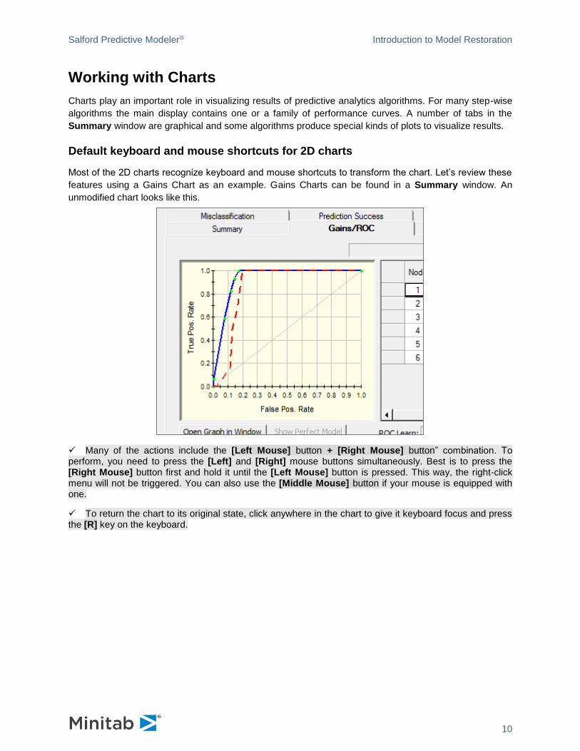
Working with Charts
Charts play an important role in visualizing results of predictive analytics algorithms. For many step-wise
algorithms the main display contains one or a family of performance curves. A number of tabs in the
Summary window are graphical and some algorithms produce special kinds of plots to visualize results.
Default keyboard and mouse shortcuts for 2D charts
Most of the 2D charts recognize keyboard and mouse shortcuts to transform the chart. Let’s review these
features using a Gains Chart as an example. Gains Charts can be found in a Summary window. An
unmodified chart looks like this.
✓ Many of the actions include the [Left Mouse] button + [Right Mouse] button” combination. To perform, you need to press the [Left] and [Right] mouse buttons simultaneously. Best is to press the [Right Mouse] button first and hold it until the [Left Mouse] button is pressed. This way, the right-click menu will not be triggered. You can also use the [Middle Mouse] button if your mouse is equipped with one.
✓ To return the chart to its original state, click anywhere in the chart to give it keyboard focus and press the [R] key on the keyboard.

Salford Predictive Modeler® Introduction to Model Restoration
11
Move the chart – [Shift] button + [Left Mouse] button + [Right Mouse] button
Move the mouse to move the chart. The chart in the screenshot below was moved to the right.
Scale the chart – [Ctrl] button + [Left Mouse] button + [Right Mouse] button
Move the mouse to scale the chart. The chart in the screenshot below was scaled and then moved up
and right to see the axes origin.

Salford Predictive Modeler® Introduction to Model Restoration
12
Zoom the chart graphically – [Ctrl] button + [Left Mouse] button
Holding the [Left Mouse] button, draw a rectangle around the area of interest.
When you release the [Left Mouse] button you will get a larger picture of the selected area.
You can repeat the action again on the resulting view.
Salford Predictive Modeler® Introduction to Model Restoration
13
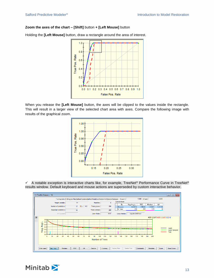
Zoom the axes of the chart – [Shift] button + [Left Mouse] button
Holding the [Left Mouse] button, draw a rectangle around the area of interest.
When you release the [Left Mouse] button, the axes will be clipped to the values inside the rectangle.
This will result in a larger view of the selected chart area with axes. Compare the following image with
results of the graphical zoom.
✓ A notable exception is interactive charts like, for example, TreeNet® Performance Curve in TreeNet® results window. Default keyboard and mouse actions are superseded by custom interactive behavior.

Salford Predictive Modeler® Introduction to Model Restoration
14
Default keyboard and mouse shortcuts for 3D charts
Most of the 3D charts recognize keyboard and mouse shortcuts to transform the chart. Let’s review these
features using a TreeNet® two variable dependency plot.
✓ Many of the actions include the [Left Mouse] button + [Right Mouse] button” combination. To perform, you need to press the [Left] and [Right] mouse buttons simultaneously. Best is to press the [Right Mouse] button first and hold it until the [Left Mouse] button is pressed. This way, the right-click menu will not be triggered. You can also use the [Middle Mouse] button if your mouse is equipped with one.
✓ To return the chart to its original state, click anywhere in the chart to give it keyboard focus and press the [R] key on the keyboard.
Rotate the chart – [Left Mouse] button + [Right Mouse] button
Press and hold both mouse buttons. A guiding cube will appear on the screen. The cube will rotate in
response to the movement of the mouse.

Salford Predictive Modeler® Introduction to Model Restoration
15
When you release both mouse buttons you will see the rotated chart.
✓ During rotation, you can press the [X], [Y] or [Z] button to rotate only around a specific axis or [E] to rotate around a custom axis. Press [N] to return to free rotation. The rotation cube shows the rotation axis if one of these keys was pressed.

Salford Predictive Modeler® Introduction to Model Restoration
16
In contrast to other transformations, the ‘R’ keyboard key does not reset the rotated chart to its original state. Most charts can be closed and reopened again to revert to the original look.
Move the chart – [Shift] button + [Left Mouse] button + [Right Mouse] button
Move the mouse to move the guiding cube. The chart in the screenshot below was moved to the right.

Salford Predictive Modeler® Introduction to Model Restoration
17
Scale the chart – [Ctrl] button + [Left Mouse] button + [Right Mouse] button
Move the mouse to scale the guiding cube. Once you release the mouse the scaled chart will appear.
Zoom the chart graphically – [Ctrl] button + [Left Mouse] button
Holding the [Left Mouse] button, draw a rectangle around the area of interest.

Salford Predictive Modeler® Introduction to Model Restoration
18
When you release the [Left Mouse] button you will get a larger picture of the selected area.
Standard right-click menu for charts
When you right-click on the chart a context menu appears.
The items on the menu allow you to perform the following actions.
Copy
Copies the image of the chart to the Clipboard.
Add To Report
Appends the image to the Report window.
Export
Exports the image of the chart to one of the supported graphical file formats.
Open in New Window
Opens a separate chart window with a copy of the chart in it.
Salford Predictive Modeler® Introduction to Model Restoration
19
Edit Chart
Shows Chart Editor for the chart.
Custom items
A chart right-click menu might have custom items. For example, the Gains Chart on the screenshot above
has a Gains Charts… menu item. It opens a Gains Charts comparison window.
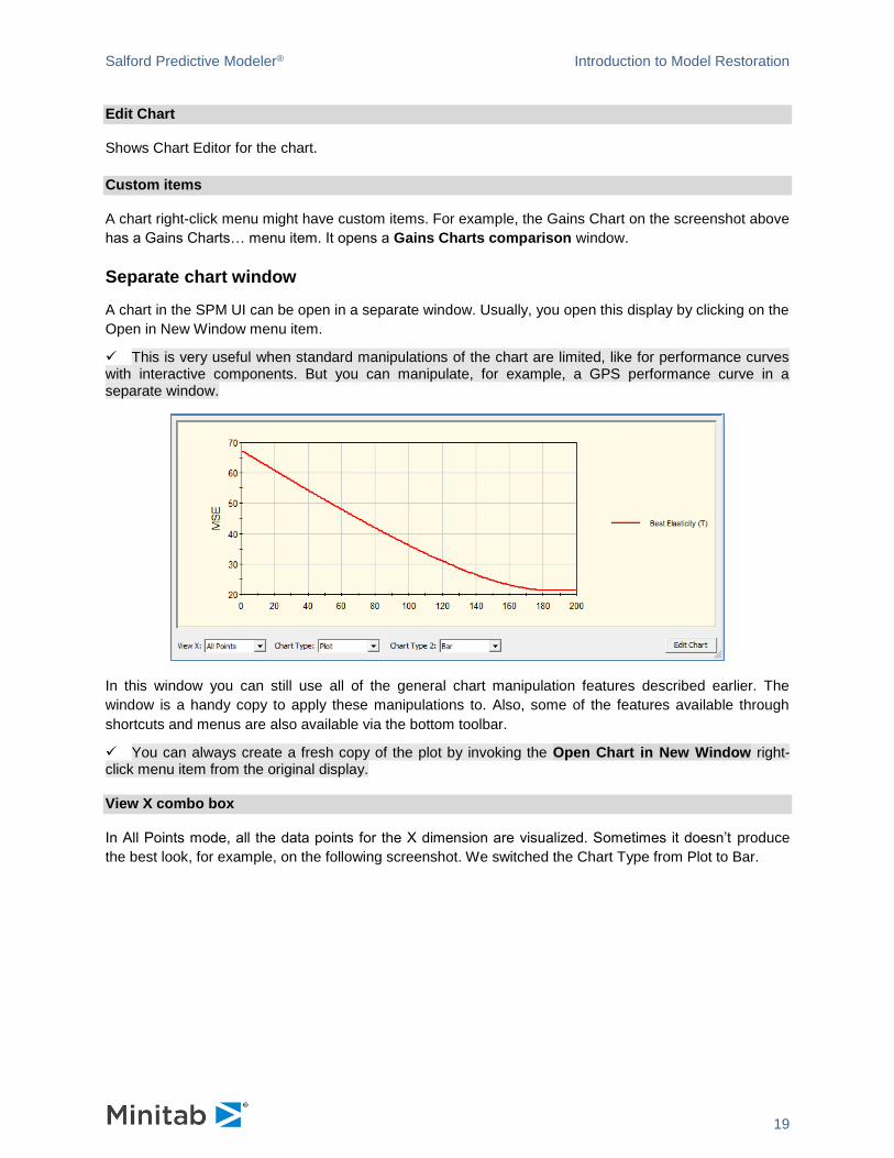
Separate chart window
A chart in the SPM UI can be open in a separate window. Usually, you open this display by clicking on the
Open in New Window menu item.
✓ This is very useful when standard manipulations of the chart are limited, like for performance curves with interactive components. But you can manipulate, for example, a GPS performance curve in a separate window.
In this window you can still use all of the general chart manipulation features described earlier. The
window is a handy copy to apply these manipulations to. Also, some of the features available through
shortcuts and menus are also available via the bottom toolbar.
✓ You can always create a fresh copy of the plot by invoking the Open Chart in New Window right-click menu item from the original display.
View X combo box
In All Points mode, all the data points for the X dimension are visualized. Sometimes it doesn’t produce
the best look, for example, on the following screenshot. We switched the Chart Type from Plot to Bar.
Salford Predictive Modeler® Introduction to Model Restoration
20
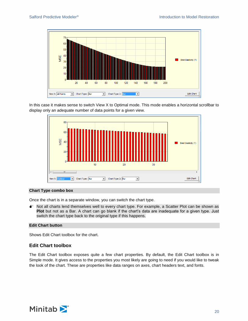
In this case it makes sense to switch View X to Optimal mode. This mode enables a horizontal scrollbar to
display only an adequate number of data points for a given view.
Chart Type combo box
Once the chart is in a separate window, you can switch the chart type.
Not all charts lend themselves well to every chart type. For example, a Scatter Plot can be shown as Plot but not as a Bar. A chart can go blank if the chart’s data are inadequate for a given type. Just switch the chart type back to the original type if this happens.
Edit Chart button
Shows Edit Chart toolbox for the chart.
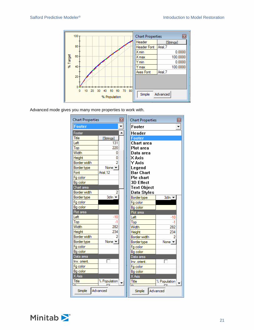
Edit Chart toolbox
The Edit Chart toolbox exposes quite a few chart properties. By default, the Edit Chart toolbox is in
Simple mode. It gives access to the properties you most likely are going to need if you would like to tweak
the look of the chart. These are properties like data ranges on axes, chart headers text, and fonts.
Salford Predictive Modeler® Introduction to Model Restoration
21
Advanced mode gives you many more properties to work with.

Salford Predictive Modeler® Introduction to Model Restoration
22
The combo box at the top helps navigating to a particular section. The changes you make are
immediately reflected on the chart associated with the toolbox.
Working with Grids
All the predictive modeling artifacts are ultimately numeric results. Many of these results can be effectively
represented as a table. Thus, grid controls are employed quite heavily in the application. For example, the
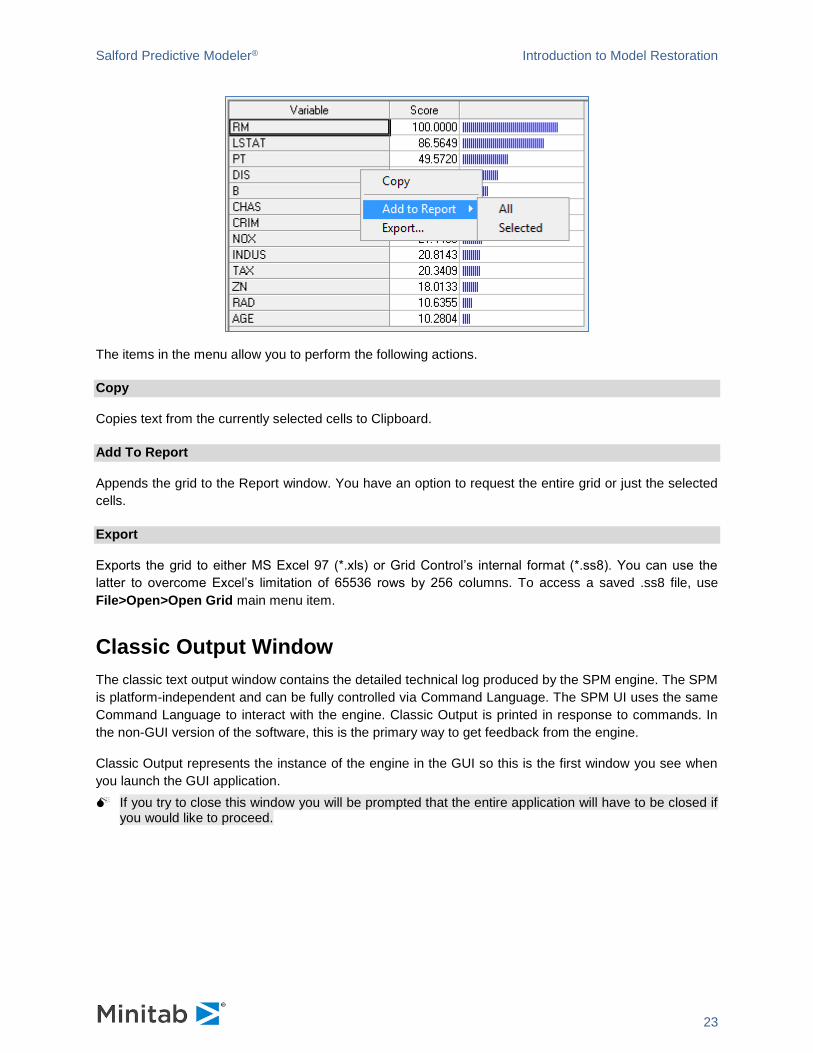
grid below shows Scores of Variable Importance in the model.
You can click on the title of any column to sort it in Ascending or Descending order. A sort indicator will
appear in the title of the column sorted. For example, a click on the Variable column will sort the grid by
Variable name.
Standard right-click menu for grids
When you right-click on the grid, a context menu appears:
Salford Predictive Modeler® Introduction to Model Restoration
23
The items in the menu allow you to perform the following actions.
Copy
Copies text from the currently selected cells to Clipboard.
Add To Report
Appends the grid to the Report window. You have an option to request the entire grid or just the selected
cells.
Export
Exports the grid to either MS Excel 97 (*.xls) or Grid Control’s internal format (*.ss8). You can use the
latter to overcome Excel’s limitation of 65536 rows by 256 columns. To access a saved .ss8 file, use
File>Open>Open Grid main menu item.
Classic Output Window
The classic text output window contains the detailed technical log produced by the SPM engine. The SPM
is platform-independent and can be fully controlled via Command Language. The SPM UI uses the same
Command Language to interact with the engine. Classic Output is printed in response to commands. In
the non-GUI version of the software, this is the primary way to get feedback from the engine.
Classic Output represents the instance of the engine in the GUI so this is the first window you see when
you launch the GUI application.
If you try to close this window you will be prompted that the entire application will have to be closed if you would like to proceed.

Salford Predictive Modeler® Introduction to Model Restoration
24
Classic Output is the first item in the application’s Window menu and you can always bring it up using
the [Ctrl]+[Alt]+[C] keyboard shortcut.
The right-hand pane of the window is a text editor that works like a console window. It has a reduced set
of features available in a Notepad window. You have an option to enable the command prompt to type
commands directly into the Classic Output window via the File>Command Prompt menu item or the
toolbar button. Whether an interactive prompt is enabled or not, the engine prints out all commands
issued to it. Each command is prepended with the ‘>’ symbol. On the screenshot below you can see
commands to setup a CART® model that uses MV (Boston Housing Dataset) as a Target variable. The
cursor is at the prompt where you can, for example, type CART® GO to start the analysis. The effect will
be the same if you run a CART® model from the GUI.

Salford Predictive Modeler® Introduction to Model Restoration
25
For your convenience, the Classic Output window is editable. You can add and remove text anywhere and even remove the prompt symbol itself. In this case it is useful to know that when you press Enter after the last line of the editor, that line is passed to the engine as a command. Alternatively, you can use the File>Command Prompt menu or toolbar button to disable and enable the command prompt again.
Report Contents pane
The left-hand pane of the Classic Output window is Report Contents. It provides useful navigation links
into the console output on the right, structured by model and organized into sections. The screenshot
below is produced by running a TreeNet® logistic binary model.
✓ You can always regenerate most of the classic output from a model saved into a Grove file by using the TRANSLATE facility built into every grove.
Salford Predictive Modeler® Introduction to Model Restoration
26
Saving Classic Output
Some models can generate an excessive amount of output. Showing it all in the Classic Output window
will eventually put considerable pressure on the UI sub-system of the OS. As a safeguard against UI
resource exhaustion, Classic Output will prompt you to save the captured output after it reaches 1 million
lines. After you confirm, the output will be preserved in the file of your choice and the window will be
cleared to receive more output. If you would like to ensure that a lengthy job runs uninterrupted, you
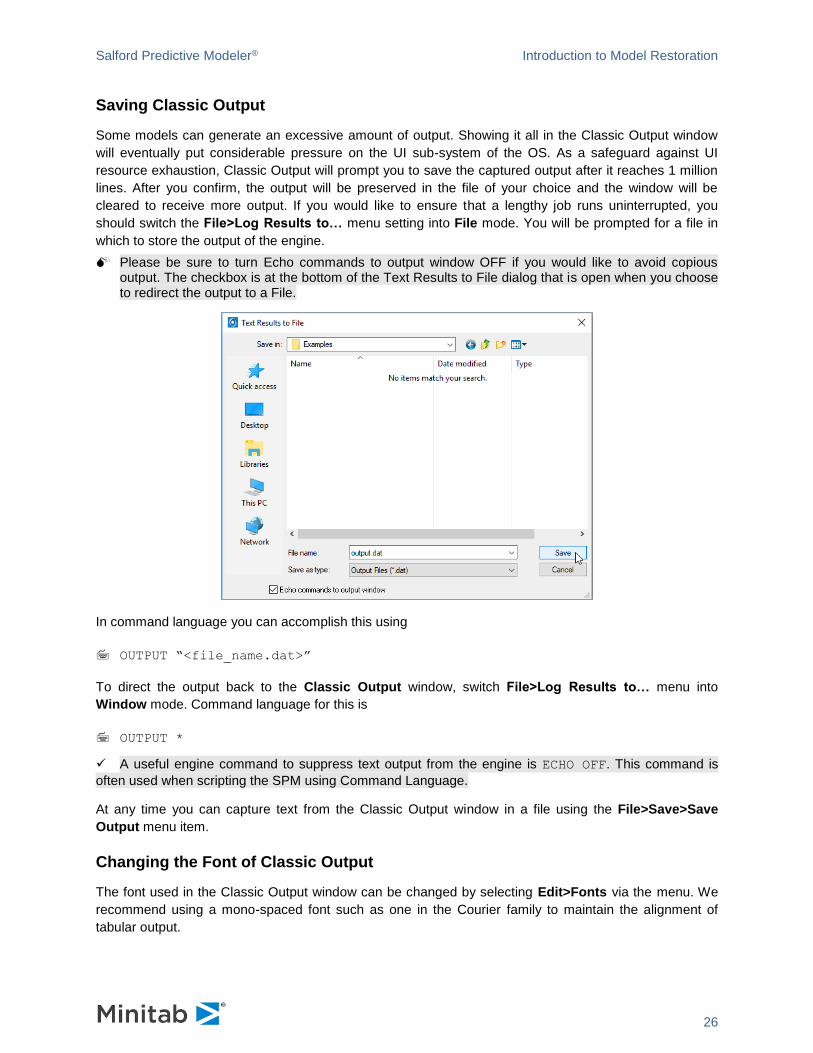
should switch the File>Log Results to… menu setting into File mode. You will be prompted for a file in
which to store the output of the engine.
Please be sure to turn Echo commands to output window OFF if you would like to avoid copious output. The checkbox is at the bottom of the Text Results to File dialog that is open when you choose to redirect the output to a File.
In command language you can accomplish this using
OUTPUT “<file_name.dat>”
To direct the output back to the Classic Output window, switch File>Log Results to… menu into
Window mode. Command language for this is
OUTPUT *
✓ A useful engine command to suppress text output from the engine is ECHO OFF. This command is
often used when scripting the SPM using Command Language.
At any time you can capture text from the Classic Output window in a file using the File>Save>Save
Output menu item.
Changing the Font of Classic Output
The font used in the Classic Output window can be changed by selecting Edit>Fonts via the menu. We
recommend using a mono-spaced font such as one in the Courier family to maintain the alignment of
tabular output.
Salford Predictive Modeler® Introduction to Model Restoration
27
Report Writer
The SPM includes a facility called Report Writer. This is a report generator, word processor and text editor. It allows you to construct custom reports from results, diagrams, tables and graphs as well as the “classic” SPM’s output appearing in the Classic Output window.
Using the Report Writer is easy! One way is to copy certain reports and diagrams to the Report window
as you view the SPM results dialog or output windows. Once processing is complete, a SPM results
window appears, allowing you to explore the performance with a variety of graphic reports, statistics, and
diagrams. Virtually any graph, table, grid display, or diagram can be copied to the Report Writer. Simply
right-click the item you wish to add to the Report Writer and select Add to Report. The selection will be
appended to the content in the Report window.
The SPM also produces Classic output for those users more comfortable with a text-based summary of
the model and its performance. To add any (or all) of the SPM’s classic output to the Report window,
highlight text in the Classic Output window, copy it to the Windows clipboard (Ctrl+C), switch to the
Report window and paste (Ctrl+V) at the point you want the text inserted. Thus, you can combine those
SPM result elements you find most useful—either graphic in nature and originating in the SPM results
dialog, or textual in nature from the Classic Output – into a single custom report.
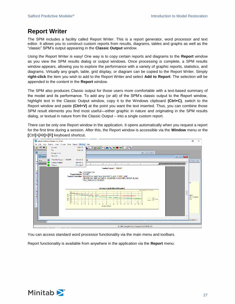
There can be only one Report window in the application. It opens automatically when you request a report
for the first time during a session. After this, the Report window is accessible via the Window menu or the
[Ctrl]+[Alt]+[R] keyboard shortcut.
You can access standard word processor functionality via the main menu and toolbars.
Report functionality is available from anywhere in the application via the Report menu:
Salford Predictive Modeler® Introduction to Model Restoration
28
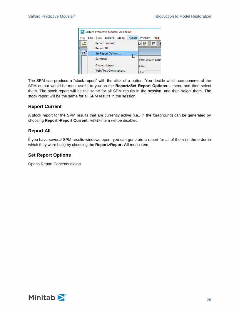
The SPM can produce a “stock report” with the click of a button. You decide which components of the
SPM output would be most useful to you on the Report>Set Report Options… menu and then select
them. The stock report will be the same for all SPM results in the session. and then select them. The
stock report will be the same for all SPM results in the session.
Report Current
A stock report for the SPM results that are currently active (i.e., in the foreground) can be generated by
choosing Report>Report Current.  item will be disabled.
Report All
If you have several SPM results windows open, you can generate a report for all of them (in the order in
which they were built) by choosing the Report>Report All menu item.
Set Report Options
Opens Report Contents dialog.
Salford Predictive Modeler® Introduction to Model Restoration
29
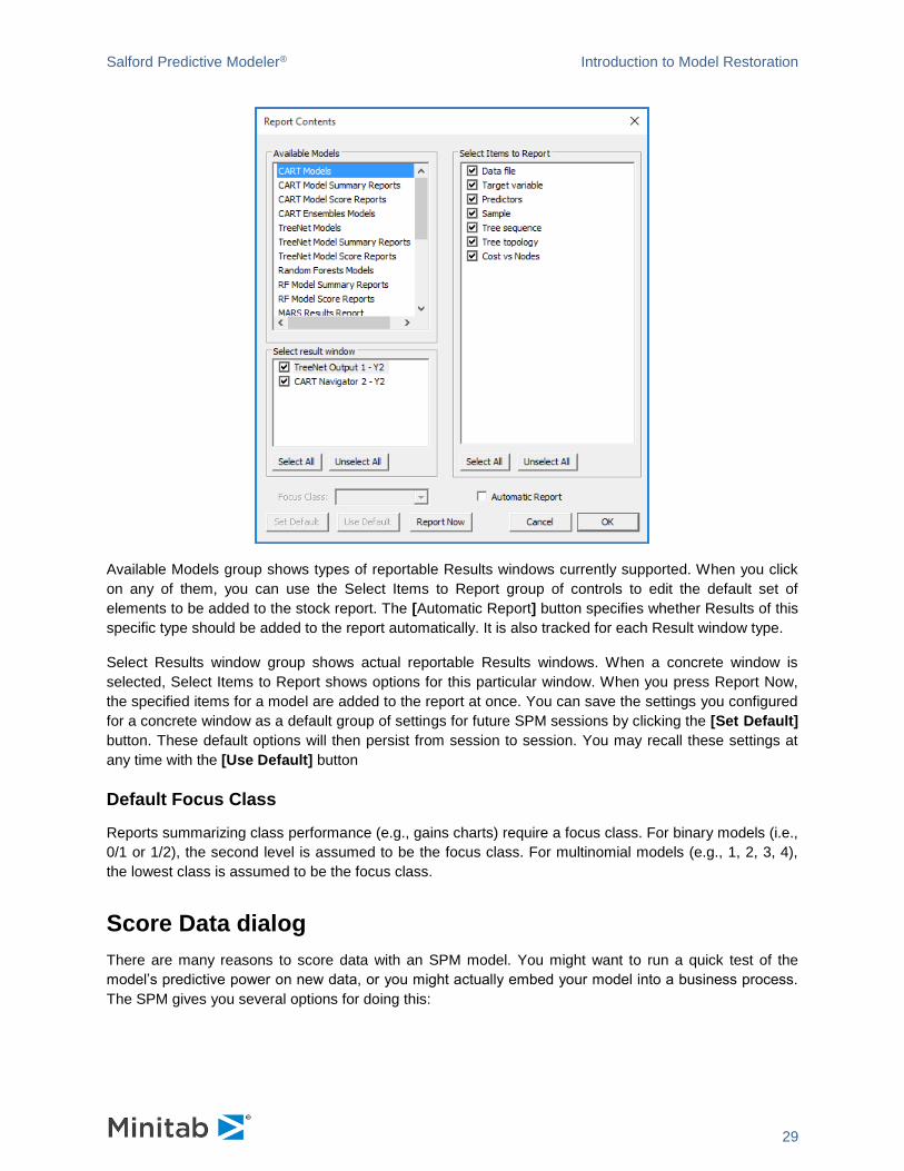
Available Models group shows types of reportable Results windows currently supported. When you click
on any of them, you can use the Select Items to Report group of controls to edit the default set of
elements to be added to the stock report. The [Automatic Report] button specifies whether Results of this
specific type should be added to the report automatically. It is also tracked for each Result window type.
Select Results window group shows actual reportable Results windows. When a concrete window is
selected, Select Items to Report shows options for this particular window. When you press Report Now,
the specified items for a model are added to the report at once. You can save the settings you configured
for a concrete window as a default group of settings for future SPM sessions by clicking the [Set Default]
button. These default options will then persist from session to session. You may recall these settings at
any time with the [Use Default] button
Default Focus Class
Reports summarizing class performance (e.g., gains charts) require a focus class. For binary models (i.e.,
0/1 or 1/2), the second level is assumed to be the focus class. For multinomial models (e.g., 1, 2, 3, 4),
the lowest class is assumed to be the focus class.
Score Data dialog
There are many reasons to score data with an SPM model. You might want to run a quick test of the
model’s predictive power on new data, or you might actually embed your model into a business process.
The SPM gives you several options for doing this:
Salford Predictive Modeler® Introduction to Model Restoration
30
The SPM can score data from any source using any previously-built SPM model. All you need to do is to attach to your data source, let the SPM know which grove file to use, and decide where you want the results to be stored.
The SPM scoring engines are available for deployment on high performance servers that can rapidly process millions of records in batch processes.
You can TRANSLATE your model into one of several programming languages including C, SAS, Java and PMML. The code produced needs little or no modification and is ready to be run in the target environment.
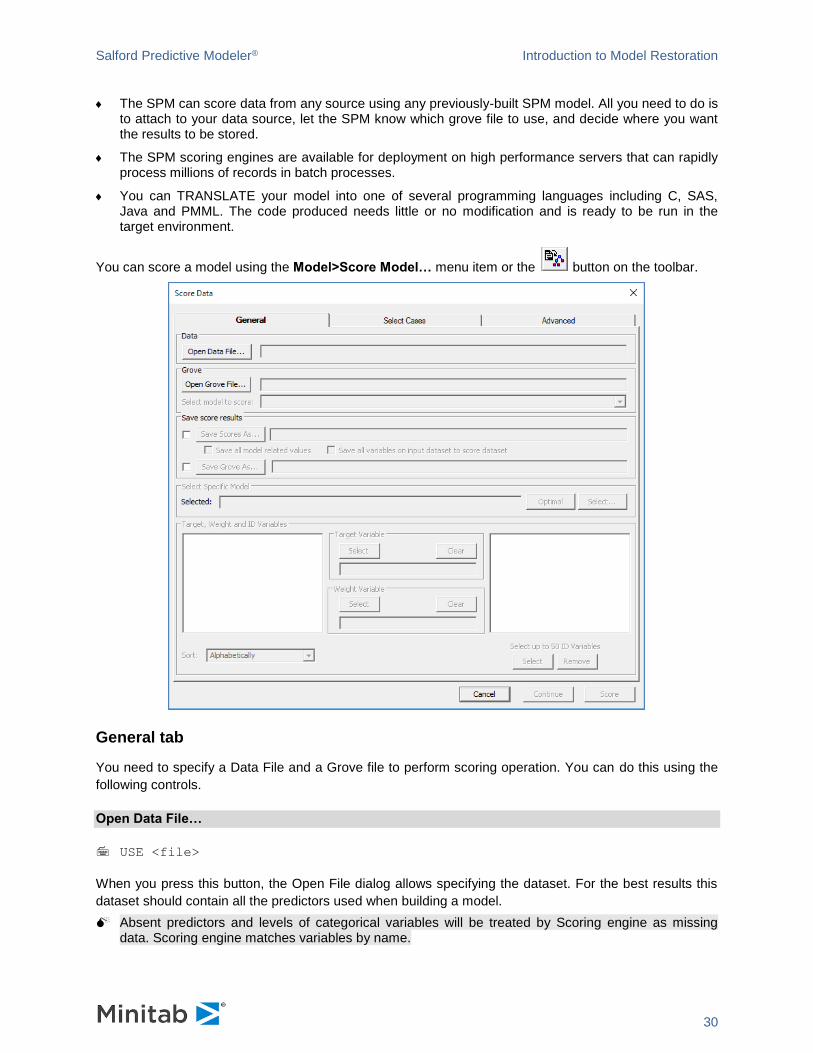
You can score a model using the Model>Score Model… menu item or the button on the toolbar.
General tab
You need to specify a Data File and a Grove file to perform scoring operation. You can do this using the
following controls.
Open Data File…
USE <file>
When you press this button, the Open File dialog allows specifying the dataset. For the best results this
dataset should contain all the predictors used when building a model.
Absent predictors and levels of categorical variables will be treated by Scoring engine as missing data. Scoring engine matches variables by name.
Salford Predictive Modeler® Introduction to Model Restoration
31
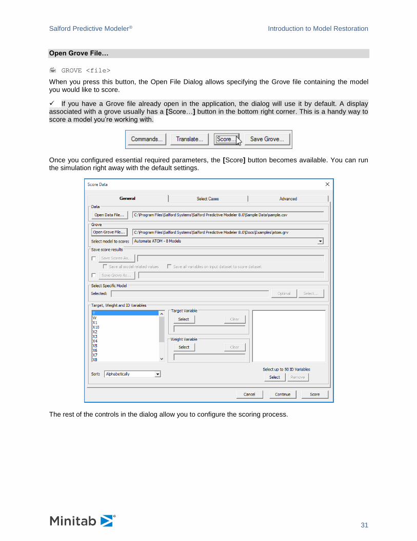
Open Grove File…
GROVE <file>
When you press this button, the Open File Dialog allows specifying the Grove file containing the model you would like to score.
✓ If you have a Grove file already open in the application, the dialog will use it by default. A display associated with a grove usually has a [Score…] button in the bottom right corner. This is a handy way to score a model you’re working with.
Once you configured essential required parameters, the [Score] button becomes available. You can run the simulation right away with the default settings.
The rest of the controls in the dialog allow you to configure the scoring process.
Salford Predictive Modeler® Introduction to Model Restoration
32
Select model to score
HARVEST ENGINE=<Engine Name>, SELECT <Model Selection parameters>
A Grove file may contain multiple models. For example, on the screenshot above the grove contains 8
models produced as a result of AUTOMATE ATOM. Using this combo box, you can either specify an
individual model or request to score all the models at once as an ensemble.
✓ HARVEST command is quite versatile and flexible. To make good use of it, please check the
documentation.
Select Specific Model
HARVEST PRUNE <Model Specific parameters>
Many of the algorithms produce a group of related models. These models represent various tradeoffs
between simplicity and accuracy. For more details, please see documentation on a specific algorithm
(CART®, TreeNet, etc.). Select Specific Model group of controls allows you to either request an optimal
model to be scored or invoke a model-specific selection dialog.
Save Scores As
SAVE <file> [MODEL, COMPLETE]
You can specify that you would like raw scores to be saved in a dataset. You can request additional data
to be saved for each observation, along with the raw scores. Save all model related values instructs the
engine to save model-specific data. For example, classification models can produce class probabilities.
Save all variables on input dataset to score dataset adds all the variables used to construct the model to
the resulting dataset. Target, Weight and ID Variables group gives a more flexible, alternative way to
handle variables in the simulation dataset.
Save Grove As
SCORE GROVE=<file>
Scoring engine produces descriptive information about the simulation (Performance Stats, Prediction
Success table, etc.). All these results are displayed in the GUI and can be saved into a Grove file for later
reference.
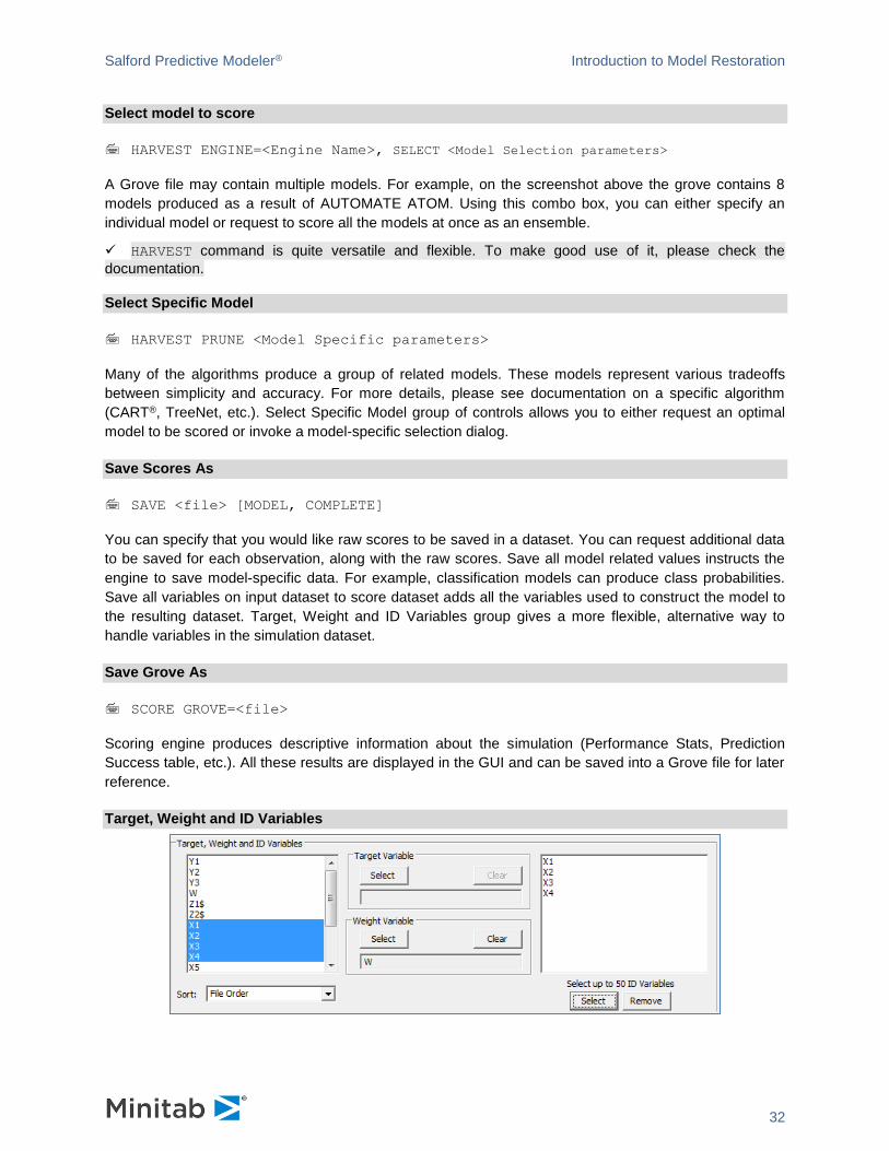
Target, Weight and ID Variables

Salford Predictive Modeler® Introduction to Model Restoration
33
The list on the left-hand side contains all the variables in the simulation dataset. The controls in the group
allow you to include specific variables into the resulting dataset and assign specific roles to them.
Target Variable
SCORE DEPVAR=<variable>
Specifies which variable in the source dataset contains actual values of the Target variable. When actual
Target is available, the Scoring engine can produce scoring performance measures. If available, actual
target variable is saved to the resulting dataset.
✓ By default, the engine matches the Target variable by name.
Weight Variable
WEIGHT <variable>
You can use a variable to identify Case Weights during simulation.
ID Variables
IDVAR <var1>, <var2>, ....
Allows you to specify which variables should be included into the resulting dataset. The variable does not
necessarily have to be a variable used to build a model.
Select Cases tab
Please refer to Select Cases tab documentation for Model Setup.
Salford Predictive Modeler® Introduction to Model Restoration
34
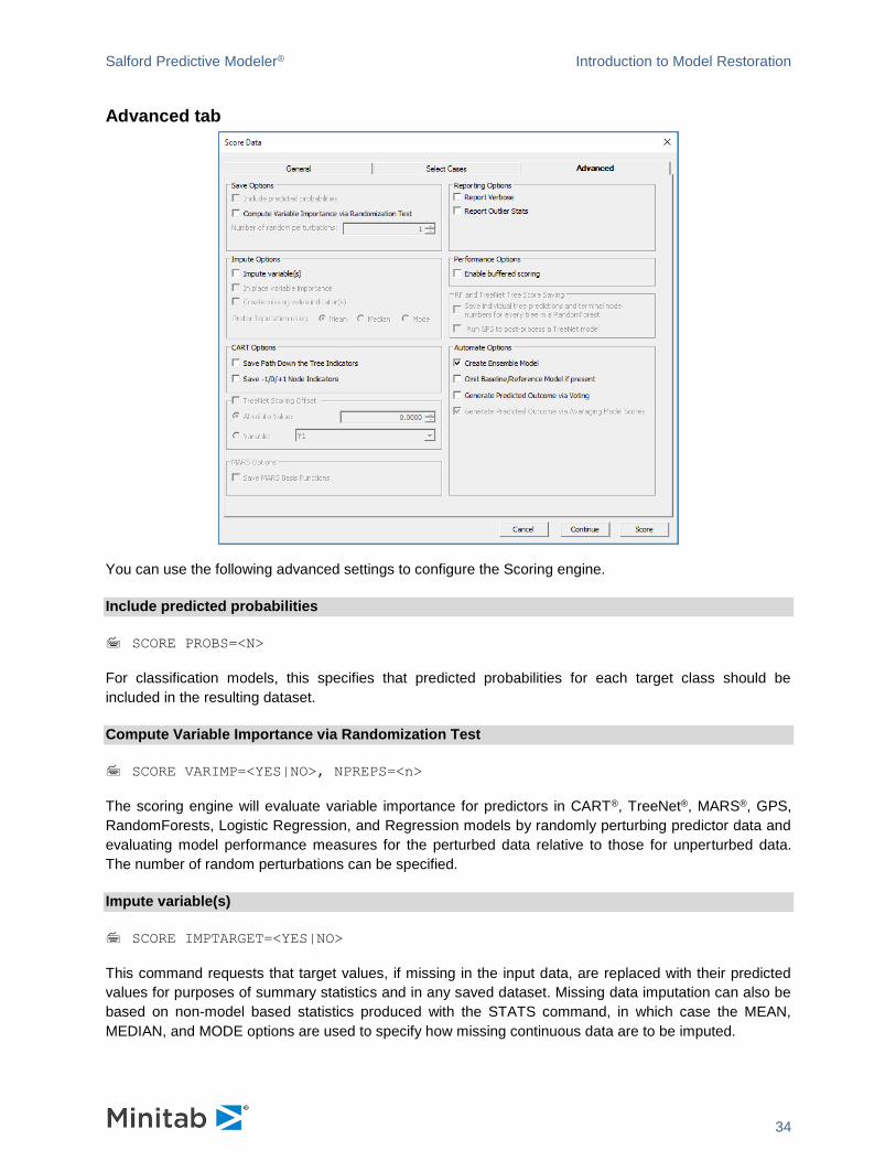
Advanced tab
You can use the following advanced settings to configure the Scoring engine.
Include predicted probabilities
SCORE PROBS=<N>
For classification models, this specifies that predicted probabilities for each target class should be
included in the resulting dataset.
Compute Variable Importance via Randomization Test
SCORE VARIMP=<YES|NO>, NPREPS=<n>
The scoring engine will evaluate variable importance for predictors in CART®, TreeNet®, MARS®, GPS,
RandomForests, Logistic Regression, and Regression models by randomly perturbing predictor data and
evaluating model performance measures for the perturbed data relative to those for unperturbed data.
The number of random perturbations can be specified.
Impute variable(s)
SCORE IMPTARGET=<YES|NO>
This command requests that target values, if missing in the input data, are replaced with their predicted
values for purposes of summary statistics and in any saved dataset. Missing data imputation can also be
based on non-model based statistics produced with the STATS command, in which case the MEAN,
MEDIAN, and MODE options are used to specify how missing continuous data are to be imputed.
Salford Predictive Modeler® Introduction to Model Restoration
35
In place variable importance
SCORE INPLACE=<YES|NO>
When IMPTARGET=YES, this option will control whether imputations are made “in place” or not. Missing
values will be replaced with imputations while leaving all non-missing data points unchanged. Without this
option, the original variable is unchanged and an imputed version of the variable is added to the output
dataset.
Create missing value indicator(s)
SCORE MVI=<YES|NO>
When IMPTARGET=YES, this option can be used to create an additional “missing value indicator”
variable that flags whether the original value was missing or not (i.e. was it imputed).
CART® Options – Save "Path Down the Tree" Indicators
SCORE PATH =<YES|NO>
For CART® models, requests that for each observation an index is recorded of each node the observation
is assigned to. Variables in form PATH_<number> are added to the output dataset. Each column contains
either
1-based index of an intermediate node.
A negative number, the absolute value of which is a 1-based index of a terminal node.
0 to indicate no node assignment. Used as a placeholder after an assignment to a terminal node is recorded.
CART® Options – Save -1/0/+1 Node Indicators
SCORE ND=<YES|NO>
For CART® models, requests that node dummies be added to the output dataset.
TreeNet® Scoring Offset
SCORE OFFSET=<x>
OFFSET defines an "offset value" for binary and regression TreeNet® models. It is similar to the INIT
option but is specified as a literal value (not a variable name).
SCORE INIT=<variable>
INIT defines a "start value" for binary and regression TreeNet® models. It is the scoring counterpart to the
TREENET INIT option used when building the model. INIT is a variable on your dataset, while OFFSET is
a literal value.
Save MARS® Basis Functions
SCORE BASIS=<YES|NO>
Salford Predictive Modeler® Introduction to Model Restoration
36
This option adds values for each of the basis functions in a MARS® model to the output dataset. This
allows the possibility for a rich set of second-stage models.
Report Verbose
SCORE IMPUTE=<YES|NO>, MEAN | MEDIAN | MODE, VERBOSE
Requests that target values, if missing in the input data, are replaced with their predicted values for
purposes of summary statistics and in any saved dataset.
Report Outlier Stats
SCORE OUTLIER=<YES|NO>
Produces several tables in Classic Output showing model performance measures as a function of outlier
trimming.
Performance Options – Enable buffered scoring
SCORE BUFFERED=<YES|NO>
The Scoring engine will score each model separately, passing once through the dataset for each model,
and will reconcile all the model scores in a post-processing step. Use this option to minimize the memory
footprint of your scoring process for large groves with many models to score.
Save individual tree predictions and terminal node numbers for every tree in a RandomForest
SCORE TREESCORES=<YES|NO>, TREENODES=<YES|NO>
For classification and regression RandomForests models, this command requests that predictions of each
tree and terminal node numbers are saved along with the prediction of the forest.
Run GPS to post-process a TreeNet® model
SCORE GPS=<YES|NO>
Builds a second-stage pipeline model on the TreeNet® model, using options on the GPS command.
Automate Options – Create Ensemble Model
SCORE ENSEMBLE=<YES|NO>
If a grove contains more than one model you can request whether they will be scored together as an
ensemble or each model will be scored individually. In latter case the output dataset will contain scores
for all the models in the grove.
Automate Options – Omit Baseline/Reference Model if present
SCORE OFT=<YES|NO>
Salford Predictive Modeler® Introduction to Model Restoration
37
Some automates produce first model as a baseline to compare other models against. In most cases when
such a Grove is scored as an ensemble it is recommended to exclude the baseline from it. Turn this
option ON if you would like baseline model to be part of the ensemble.
Automate Options – Generate Predicted Outcome via Voting
Automate Options – Generate Predicted Outcome via Averaging Model Scores
SCORE TNAVERAGE=<YES|NO>
The Scoring engine will score ensembles composed of classification or logistic binary TreeNet® models in
a special way. Most categorical ensembles are scored using a voting approach, in which the predicted
class of each individual model is noted and the class with the most instances, or "votes", is determined to
be the predicted class of the ensemble as a whole. However, with classification or logistic binary
TreeNet® ensembles, another approach which is typically more accurate is used by default: the raw
scores of the individual class-specific TreeNet®s are averaged over all the models in the ensemble, and
the predicted probabilities and the class are then determined.
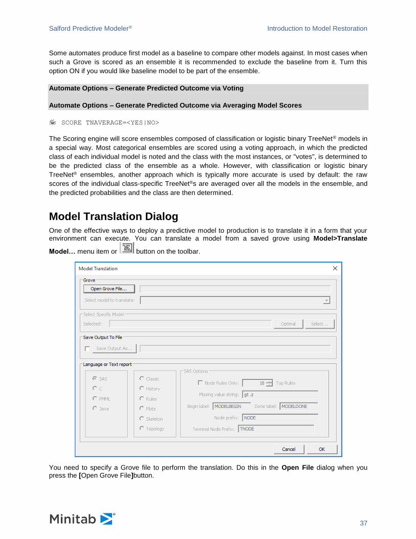
Model Translation Dialog
One of the effective ways to deploy a predictive model to production is to translate it in a form that your environment can execute. You can translate a model from a saved grove using Model>Translate
Model… menu item or button on the toolbar.
You need to specify a Grove file to perform the translation. Do this in the Open File dialog when you press the [Open Grove File]button.
Salford Predictive Modeler® Introduction to Model Restoration
38
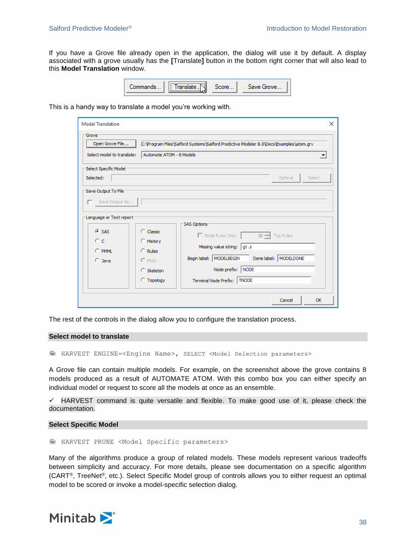
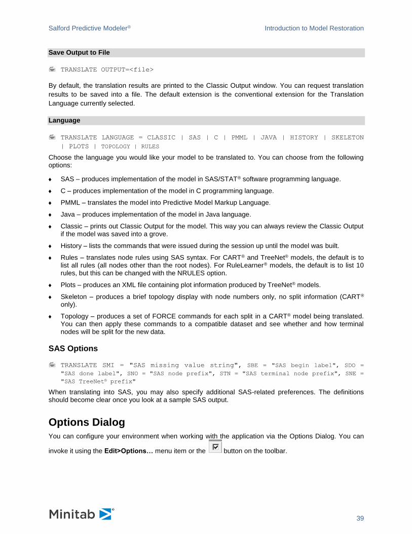
If you have a Grove file already open in the application, the dialog will use it by default. A display associated with a grove usually has the [Translate] button in the bottom right corner that will also lead to this Model Translation window.
This is a handy way to translate a model you’re working with.
The rest of the controls in the dialog allow you to configure the translation process.
Select model to translate
HARVEST ENGINE=<Engine Name>, SELECT <Model Selection parameters>
A Grove file can contain multiple models. For example, on the screenshot above the grove contains 8
models produced as a result of AUTOMATE ATOM. With this combo box you can either specify an
individual model or request to score all the models at once as an ensemble.
✓ HARVEST command is quite versatile and flexible. To make good use of it, please check the documentation.
Select Specific Model
HARVEST PRUNE <Model Specific parameters>
Many of the algorithms produce a group of related models. These models represent various tradeoffs
between simplicity and accuracy. For more details, please see documentation on a specific algorithm
(CART®, TreeNet®, etc.). Select Specific Model group of controls allows you to either request an optimal
model to be scored or invoke a model-specific selection dialog.
Salford Predictive Modeler® Introduction to Model Restoration
39
Save Output to File
TRANSLATE OUTPUT=<file>
By default, the translation results are printed to the Classic Output window. You can request translation
results to be saved into a file. The default extension is the conventional extension for the Translation
Language currently selected.
Language
TRANSLATE LANGUAGE = CLASSIC | SAS | C | PMML | JAVA | HISTORY | SKELETON
| PLOTS | TOPOLOGY | RULES
Choose the language you would like your model to be translated to. You can choose from the following options:
SAS – produces implementation of the model in SAS/STAT® software programming language.
C – produces implementation of the model in C programming language.
PMML – translates the model into Predictive Model Markup Language.
Java – produces implementation of the model in Java language.
Classic – prints out Classic Output for the model. This way you can always review the Classic Output if the model was saved into a grove.
History – lists the commands that were issued during the session up until the model was built.
Rules – translates node rules using SAS syntax. For CART® and TreeNet® models, the default is to list all rules (all nodes other than the root nodes). For RuleLearner® models, the default is to list 10 rules, but this can be changed with the NRULES option.
Plots – produces an XML file containing plot information produced by TreeNet® models.
Skeleton – produces a brief topology display with node numbers only, no split information (CART® only).
Topology – produces a set of FORCE commands for each split in a CART® model being translated. You can then apply these commands to a compatible dataset and see whether and how terminal nodes will be split for the new data.
SAS Options
TRANSLATE SMI = "SAS missing value string", SBE = "SAS begin label", SDO =
"SAS done label", SNO = "SAS node prefix", STN = "SAS terminal node prefix", SNE =
"SAS TreeNet® prefix"
When translating into SAS, you may also specify additional SAS-related preferences. The definitions should become clear once you look at a sample SAS output.
Options Dialog
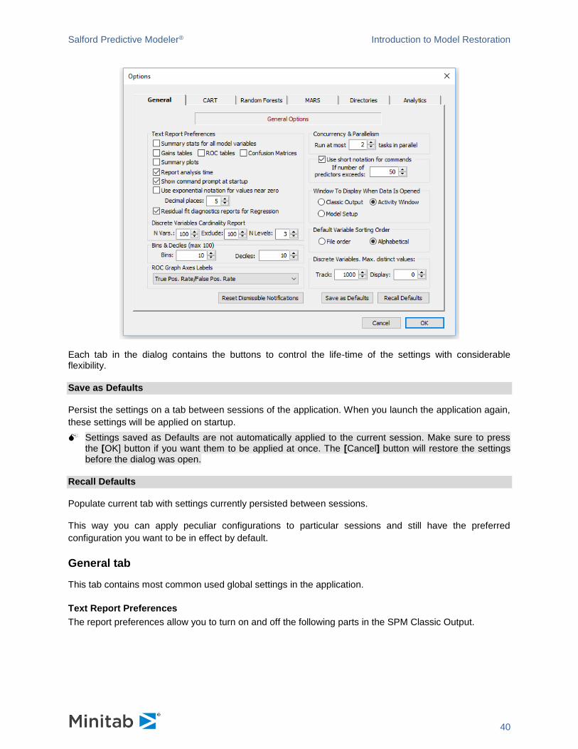
You can configure your environment when working with the application via the Options Dialog. You can
invoke it using the Edit>Options… menu item or the button on the toolbar.
Salford Predictive Modeler® Introduction to Model Restoration
40
Each tab in the dialog contains the buttons to control the life-time of the settings with considerable flexibility.
Save as Defaults
Persist the settings on a tab between sessions of the application. When you launch the application again,
these settings will be applied on startup.
Settings saved as Defaults are not automatically applied to the current session. Make sure to press the [OK] button if you want them to be applied at once. The [Cancel] button will restore the settings before the dialog was open.
Recall Defaults
Populate current tab with settings currently persisted between sessions.
This way you can apply peculiar configurations to particular sessions and still have the preferred
configuration you want to be in effect by default.
General tab
This tab contains most common used global settings in the application.
Text Report Preferences
The report preferences allow you to turn on and off the following parts in the SPM Classic Output.
Salford Predictive Modeler® Introduction to Model Restoration
41
Summary stats for all model variables
LOPTIONS MEANS=<YES|NO>
Report the summary statistics including mean, standard deviation, minimum, maximum, etc. In
classification models, the stats are reported for the overall train and test samples and then separately for
each level of the target.
Gains tables
LOPTIONS GAINS=<YES|NO>
Report Gains tables for CART® classification models.
ROC tables
LOPTIONS ROC=<YES|NO>
Report ROC tables for CART® classification models.
Confusion Matrices (prediction success tables)
LOPTIONS CONFUSION_MATRIX=<YES|NO> / [CLASS|PROB|BOTH]
LOPTIONS PREDICTION_SUCCESS=<YES|NO> / [CLASS|PROB|BOTH]
Report Confusion Matrix with misclassification counts and percents by class level. For some reports, two
tables are available: one based on class predictions and one based on predicted probabilities. You can
control them individually or request both.
Summary plots
LOPTIONS PLOTS=<YES|NO> / “<plot_character>”
Enables summary plots in the text output and allows a user-specified plotting symbol.
Report analysis time
LOPTIONS TIMING=<YES|NO>
Report CPU time required for each stage of the analysis.
Use exponential notation for values near zero / Decimal places
FORMAT=<#> / UNDERFLOW
Precision to which the numerical output is printed. This will affect all the UI as well as text output from the
engine after this option is applied. The UNDERFLOW option prints tiny numbers in scientific notation.
Residual fit diagnostics reports for Regression

Salford Predictive Modeler® Introduction to Model Restoration
42
LOPTIONS RESIDUALDIAG=<YES|NO>
Enables or suppresses residual model fit diagnostic reports for regression models only.
Other Controls
ROC Graph Labels
ROC graphs are traditionally labeled differently in different industries. You can select from the two labeling schemes displayed below:
Concurrency & Parallelism
THREADS=<n>
Specifies maximal degree of parallelism (maximal number of worker threads permitted to run in the
application). By default, the GUI application uses number of physical cores (not hyperthreading cores) on
the machine.
In our experience setting a number of tasks to run in parallel higher than the number of physical cores may significantly degrade performance.
Use Short Command Notation
Sets the minimal number of predictors that triggers a short command notation in the command log. When
the number of predictors is small, each predictor is printed in the command log (for example, KEEP or
CATEGORY commands). However, when the number of predictors exceeds the limit, the SPM uses
“dash” convention to indicate ranges of predictors (for example, X1-X5).
✓ This setting only affects how the GUI generates commands. The command parser supports both short and standard command notations.
Window to Display When Data Is Opened
When you open a data file, the SPM gives you three choices for what to do next:
Classic Output – use this if you don’t want any task-specific dialogs to pop up as soon as a dataset is open. Useful when authoring command files.
Activity Window – this dialog gives you a convenient way to access common data mining tasks once a new dataset is open.
Model Setup – in many common analysis scenarios, the window to navigate to from the Activity Window is Model Setup. For convenience, you have an option to bypass the Activity Window for a newly open dataset.
Default Variable Sorting Order
Many GUI displays include a list of variables and you can always change the sort order between
Alphabetical and File Order (the order in which the variables appear in your data file). This setting allows
you to determine the ordering that will always show first when a dialog is opened.

Salford Predictive Modeler® Introduction to Model Restoration
43
Algorithm-specific tabs
Please refer to documentation on a specific algorithm (CART®, TreeNet®, etc.) for information about tabs
with algorithm-specific options. The settings on these tabs are usually configured for a newly installed
instance of the application and only changed rarely, if ever, after that. In contrast, the Model Setup dialog
contains settings that are likely to change for every engine run.
Directories tab
This tab allows you to setup working directories. The SPM gives you flexibility to specify working directories for different categories of files.
Input Files Locations
By default, the SPM GUI looks for files at the following locations:
Data – datasets for modeling.
Model information – previously-saved the SPM model files.
Command – command files or scripts.
Output Files Locations
By default, the SPM GUI writes files to the following locations:
Model information – the SPM model files saved for later scoring or export.
Prediction results – output datasets containing scores or predictions.
Run report – classic plain text output.
✓ Depending on your working style you may choose to store input and output files at the same location or use separate locations for them.
Salford Predictive Modeler® Introduction to Model Restoration
44
Temporary Files
Specifies the location where the SPM creates temporary files, including command log files for entire
application sessions.
By default the SPM queries OS for current user’s default directory for temporary files. When selecting a
directory for temporary files please take the following into consideration.
Make sure that the drive where the temporary folder is located will have enough space (at least the size of the largest data set you are planning to use).
Temporary files with names like SPMU1227120944_s2as__.txt are records of your previous sessions. The first part of the name refers to today’s date (December 27th 2012) followed by a random series of digits and letters to give the file a unique name. These command logs provide a record of what you were doing during any session and will be stored even if you experience an Operating System crash or power outage. You may find this record invaluable if you ever need to reconstruct work you were doing.
✓ You can browse these session logs using View>Past Session Logs menu.
Temporary files with names other than SPMUnnnnn.txt are normally deleted when you shut the SPM down. If you find such files in your temporary directory it is safe to delete them as they contain no useful information.
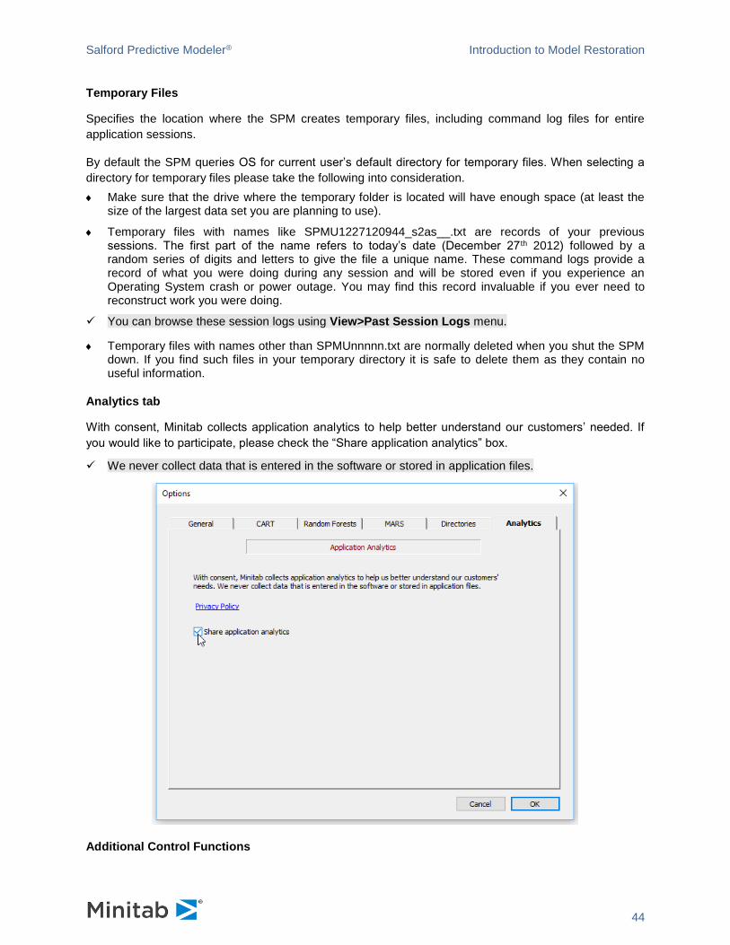
Analytics tab
With consent, Minitab collects application analytics to help better understand our customers’ needed. If
you would like to participate, please check the “Share application analytics” box.
✓ We never collect data that is entered in the software or stored in application files.
Additional Control Functions

Salford Predictive Modeler® Introduction to Model Restoration
45
–Control icon that automatically changes all path references to make them identical with the Data: entry.
–Control icon that starts the Select Default Directory dialog, allowing the user to browse for the desired directory.
–Control that allows you to select from a list of previously-used directories.
– Control that allows the user to specify how many files to show in the Most Recently Used (MRU) menu. The maximum allowable is 20 files. files. files.
Salford Predictive Modeler® Introduction to Model Restoration
46
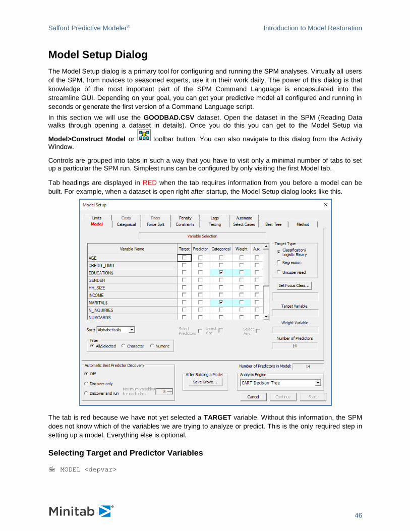
Model Setup Dialog
The Model Setup dialog is a primary tool for configuring and running the SPM analyses. Virtually all users
of the SPM, from novices to seasoned experts, use it in their work daily. The power of this dialog is that
knowledge of the most important part of the SPM Command Language is encapsulated into the
streamline GUI. Depending on your goal, you can get your predictive model all configured and running in
seconds or generate the first version of a Command Language script.
In this section we will use the GOODBAD.CSV dataset. Open the dataset in the SPM (Reading Data walks through opening a dataset in details). Once you do this you can get to the Model Setup via
Model>Construct Model or toolbar button. You can also navigate to this dialog from the Activity Window.
Controls are grouped into tabs in such a way that you have to visit only a minimal number of tabs to set up a particular the SPM run. Simplest runs can be configured by only visiting the first Model tab.
Tab headings are displayed in RED when the tab requires information from you before a model can be
built. For example, when a dataset is open right after startup, the Model Setup dialog looks like this.
The tab is red because we have not yet selected a TARGET variable. Without this information, the SPM
does not know which of the variables we are trying to analyze or predict. This is the only required step in
setting up a model. Everything else is optional.
Selecting Target and Predictor Variables
MODEL <depvar>
Salford Predictive Modeler® Introduction to Model Restoration
47
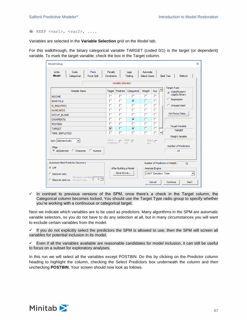
KEEP <var1>, <var2>, ....
Variables are selected in the Variable Selection grid on the Model tab.
For this walkthrough, the binary categorical variable TARGET (coded 0/1) is the target (or dependent)
variable. To mark the target variable, check the box in the Target column.
✓ In contrast to previous versions of the SPM, once there’s a check in the Target column, the Categorical column becomes locked. You should use the Target Type radio group to specify whether you’re working with a continuous or categorical target.
Next we indicate which variables are to be used as predictors. Many algorithms in the SPM are automatic
variable selectors, so you do not have to do any selection at all, but in many circumstances you will want
to exclude certain variables from the model.
✓ If you do not explicitly select the predictors the SPM is allowed to use, then the SPM will screen all variables for potential inclusion in its model.
✓ Even if all the variables available are reasonable candidates for model inclusion, it can still be useful to focus on a subset for exploratory analyses.
In this run we will select all the variables except POSTBIN. Do this by clicking on the Predictor column
heading to highlight the column, checking the Select Predictors box underneath the column and then
unchecking POSTBIN. Your screen should now look as follows.

Salford Predictive Modeler® Introduction to Model Restoration
48
✓ It is always a good idea to exclude bookkeeping columns such as ID variables. These are not suitable for prediction.
✓ You can select groups of cells with mouse and keyboard and then use checkboxes under the grid to check and uncheck boxes in all selected rows at once. The grid supports selecting nonadjacent cells when you press and hold the [Ctrl] key and adjacent cells when you press and hold the [Shift] key.
Categorical Predictors
CATEGORY <var1>, <var2>, ....
Categorical column allows you to specify which of the numeric variables are categorical by nature. Character variables, like MARITAL$, have been automatically checked as categorical. Let’s select GENDER as a numeric categorical predictor.
Salford Predictive Modeler® Introduction to Model Restoration
49
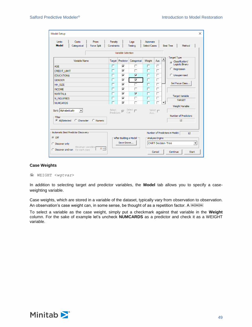
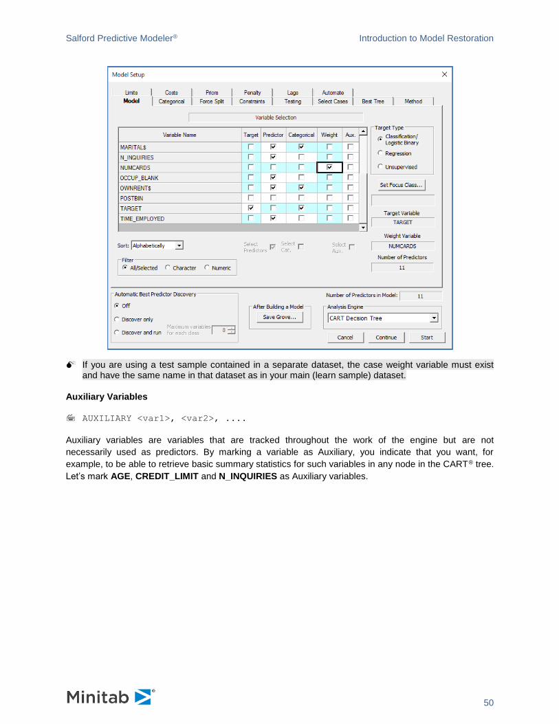
Case Weights
WEIGHT <wgtvar>
In addition to selecting target and predictor variables, the Model tab allows you to specify a case-
weighting variable.
Case weights, which are stored in a variable of the dataset, typically vary from observation to observation.
An observation’s case weight can, in some sense, be thought of as a repetition factor. A 
To select a variable as the case weight, simply put a checkmark against that variable in the Weight column. For the sake of example let’s uncheck NUMCARDS as a predictor and check it as a WEIGHT variable.
Salford Predictive Modeler® Introduction to Model Restoration
50
If you are using a test sample contained in a separate dataset, the case weight variable must exist and have the same name in that dataset as in your main (learn sample) dataset.
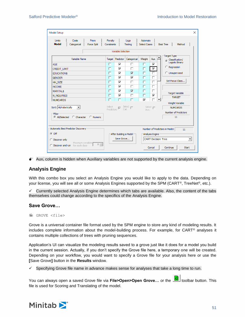
Auxiliary Variables
AUXILIARY <var1>, <var2>, ....
Auxiliary variables are variables that are tracked throughout the work of the engine but are not
necessarily used as predictors. By marking a variable as Auxiliary, you indicate that you want, for
example, to be able to retrieve basic summary statistics for such variables in any node in the CART® tree.
Let’s mark AGE, CREDIT_LIMIT and N_INQUIRIES as Auxiliary variables.
Salford Predictive Modeler® Introduction to Model Restoration
51
Aux. column is hidden when Auxiliary variables are not supported by the current analysis engine.
Analysis Engine
With this combo box you select an Analysis Engine you would like to apply to the data. Depending on
your license, you will see all or some Analysis Engines supported by the SPM (CART®, TreeNet®, etc.).
✓ Currently selected Analysis Engine determines which tabs are available. Also, the content of the tabs themselves could change according to the specifics of the Analysis Engine.
Save Grove…
GROVE <file>
Grove is a universal container file format used by the SPM engine to store any kind of modeling results. It
includes complete information about the model-building process. For example, for CART® analyses it
contains multiple collections of trees with pruning sequences.
Application’s UI can visualize the modeling results saved to a grove just like it does for a model you build
in the current session. Actually, if you don’t specify the Grove file here, a temporary one will be created.
Depending on your workflow, you would want to specify a Grove file for your analysis here or use the
[Save Grove] button in the Results window.
✓ Specifying Grove file name in advance makes sense for analyses that take a long time to run.
You can always open a saved Grove file via File>Open>Open Grove… or the toolbar button. This
file is used for Scoring and Translating of the model.

Salford Predictive Modeler® Introduction to Model Restoration
52
Automatic Best Predictor Discovery
TREENET DISCOVER = (MANUAL | AUTO)[, TOP = <n>]
You can use the TreeNet® algorithm to discover most important predictors before you run the analysis.
This could be useful if the desired Analysis Engine could benefit from narrowing down the predictor list.
Discover only will show results of the discovery and give you control to select the predictors while
Discover and run will make a selection automatically and proceed to run the analysis.
In many cases it is advisable to just run a TreeNet® model and explore its results rather than using auto-discovery. Variable Importance tab has a facility to configure the SPM engine with the list of most important predictors.
Model tab
The Variable Selection grid is described in the Selecting Target and Predictor Variables section. The tab
also has the following controls.
Setting Focus Class
In classification runs, some of the reports generated by the SPM (gains, prediction success, color-coding, etc.) have one target class in focus. By default, the SPM will put the first class it finds in the dataset in focus. A user can overwrite this by pressing the [Set Focus Class] button
Sorting Variable List
The variable list can be sorted either in physical order or alphabetically by changing the Sort: control box. Depending on the dataset, one of those modes will be preferable, which is usually helpful when dealing with large variable lists.
Specifying Target Type
The SPM uses the Target Type radio group to determine how the Target variable will be interpreted by the engine. The following Target Types are supported:
Classification/Logistic Binary – the Target is categorical or binary, may have 2 or more categories.
Regression – the Target is continuous.
Unsupervised – no Target variable is required in the data.
✓ The content of other tabs depends quite substantially on the Target Type selected.
Salford Predictive Modeler® Introduction to Model Restoration
53
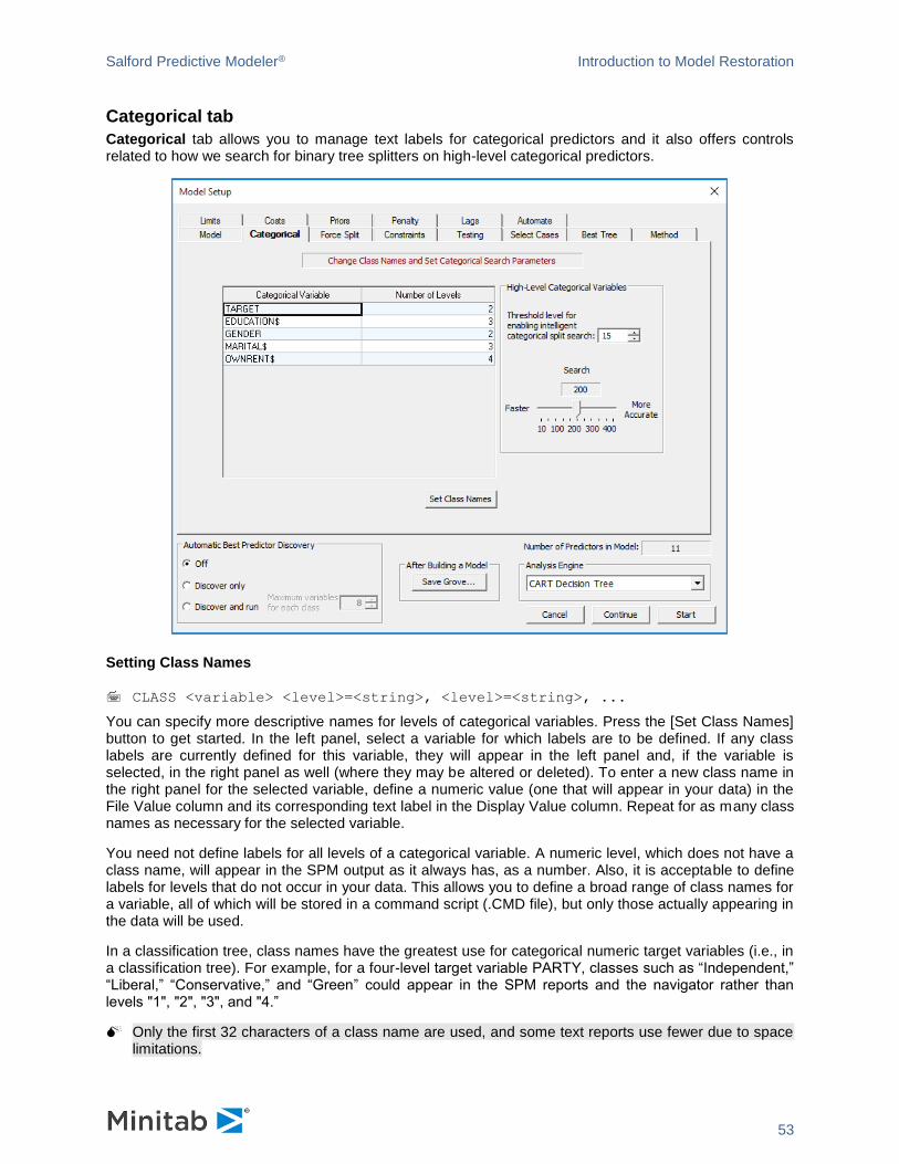
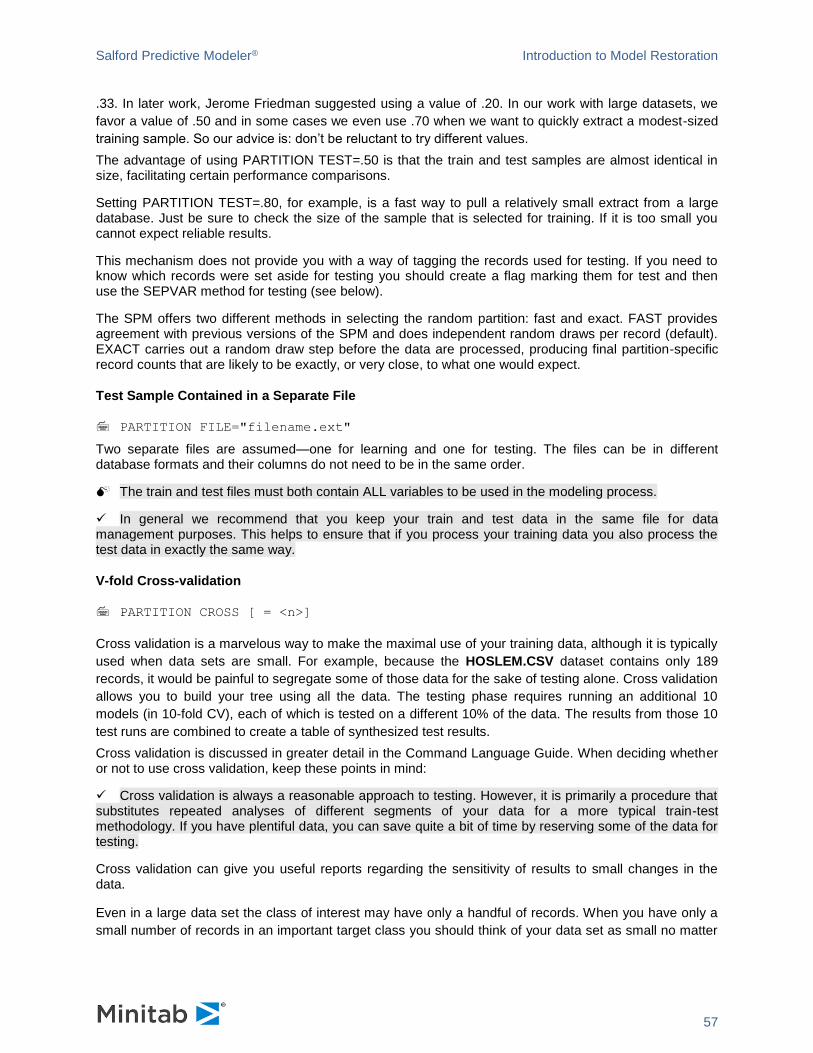
Categorical tab
Categorical tab allows you to manage text labels for categorical predictors and it also offers controls related to how we search for binary tree splitters on high-level categorical predictors.
Setting Class Names
CLASS <variable> <level>=<string>, <level>=<string>, ...
You can specify more descriptive names for levels of categorical variables. Press the [Set Class Names] button to get started. In the left panel, select a variable for which labels are to be defined. If any class labels are currently defined for this variable, they will appear in the left panel and, if the variable is selected, in the right panel as well (where they may be altered or deleted). To enter a new class name in the right panel for the selected variable, define a numeric value (one that will appear in your data) in the File Value column and its corresponding text label in the Display Value column. Repeat for as many class names as necessary for the selected variable.
You need not define labels for all levels of a categorical variable. A numeric level, which does not have a class name, will appear in the SPM output as it always has, as a number. Also, it is acceptable to define labels for levels that do not occur in your data. This allows you to define a broad range of class names for a variable, all of which will be stored in a command script (.CMD file), but only those actually appearing in the data will be used.
In a classification tree, class names have the greatest use for categorical numeric target variables (i.e., in a classification tree). For example, for a four-level target variable PARTY, classes such as “Independent,” “Liberal,” “Conservative,” and “Green” could appear in the SPM reports and the navigator rather than levels "1", "2", "3", and "4.”
Only the first 32 characters of a class name are used, and some text reports use fewer due to space limitations.

Salford Predictive Modeler® Introduction to Model Restoration
54
For example, let’s give more descriptive names to the levels of GENDER variable. The Categorical Variable Class Names dialog appears as follows.
✓ If you use the GUI to define class names and wish to reuse the class names in a future session, save the command log before exiting the SPM. Cut and paste the CLASS commands appearing in the command log into a new command file.
High-Level Categorical Predictors in Decision Trees
BOPTIONS NCLASSES=<n>
BOPTIONS HLC= <n1>, <n2>
We take great pride in noting that the SPM is capable of handling categorical predictors with thousands of
levels (given sufficient RAM workspace) when searching for a split for a decision tree. However, using
such predictors in their raw form is generally not a good idea. Rather, it is usually advisable to reduce the
number of levels by grouping or aggregating levels, as this will likely yield more reliable predictive models.
It is also advisable to impose the HLC penalty on such variables (from the Model Setup—Penalty tab).
These topics are discussed at greater length later in the Guide. In this section we discuss the simple
mechanics for handling any HLC predictors you have decided to use.
For the binary target, high-level categorical predictors pose no special computational problem as exact
short cut solutions are available and the processing time is minimal no matter how many levels there are.
For the multi-class target variable (more than two classes), we know of no similar exact short cut
methods, although research has led to substantial acceleration. HLCs present a computational challenge
because of the sheer number of possible ways to split the data in a node. The number of distinct splits
that can be generated using a categorical predictor with K levels is 2K-1 -1. If K=4, for example, the number
of candidate splits is 7; if K=11, the total is 1,023; if K=21, the number is over one million; and if K=35, the
number of splits is more than 34 billion! Naïve processing of such problems could take days, weeks,
months, or even years to complete!
Salford Predictive Modeler® Introduction to Model Restoration
55
To deal more efficiently with high-level categorical (HLC) predictors, the SPM has an intelligent search
procedure that efficiently approximates the exhaustive split search procedure normally used. The HLC
procedure can radically reduce the number of splits actually tested and still find a near optimal split for a
high-level categorical.
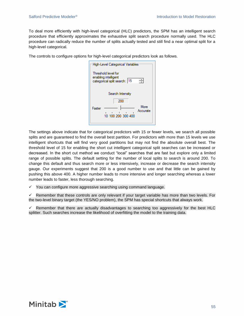
The controls to configure options for high-level categorical predictors look as follows.
The settings above indicate that for categorical predictors with 15 or fewer levels, we search all possible
splits and are guaranteed to find the overall best partition. For predictors with more than 15 levels we use
intelligent shortcuts that will find very good partitions but may not find the absolute overall best. The
threshold level of 15 for enabling the short cut intelligent categorical split searches can be increased or
decreased. In the short cut method we conduct “local” searches that are fast but explore only a limited
range of possible splits. The default setting for the number of local splits to search is around 200. To
change this default and thus search more or less intensively, increase or decrease the search intensity
gauge. Our experiments suggest that 200 is a good number to use and that little can be gained by
pushing this above 400. A higher number leads to more intensive and longer searching whereas a lower
number leads to faster, less thorough searching.
✓ You can configure more aggressive searching using command language.
✓ Remember that these controls are only relevant if your target variable has more than two levels. For the two-level binary target (the YES/NO problem), the SPM has special shortcuts that always work.
✓ Remember that there are actually disadvantages to searching too aggressively for the best HLC splitter. Such searches increase the likelihood of overfitting the model to the training data.
Salford Predictive Modeler® Introduction to Model Restoration
56
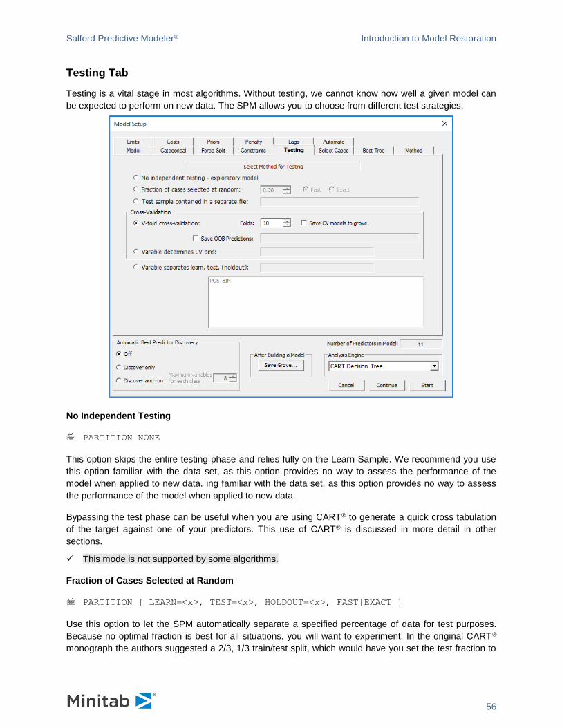
Testing Tab
Testing is a vital stage in most algorithms. Without testing, we cannot know how well a given model can
be expected to perform on new data. The SPM allows you to choose from different test strategies.
No Independent Testing
PARTITION NONE
This option skips the entire testing phase and relies fully on the Learn Sample. We recommend you use
this option familiar with the data set, as this option provides no way to assess the performance of the
model when applied to new data. ing familiar with the data set, as this option provides no way to assess
the performance of the model when applied to new data.
Bypassing the test phase can be useful when you are using CART® to generate a quick cross tabulation
of the target against one of your predictors. This use of CART® is discussed in more detail in other
sections.
✓ This mode is not supported by some algorithms.
Fraction of Cases Selected at Random
PARTITION [ LEARN=<x>, TEST=<x>, HOLDOUT=<x>, FAST|EXACT ]
Use this option to let the SPM automatically separate a specified percentage of data for test purposes.
Because no optimal fraction is best for all situations, you will want to experiment. In the original CART®
monograph the authors suggested a 2/3, 1/3 train/test split, which would have you set the test fraction to
Salford Predictive Modeler® Introduction to Model Restoration
57
.33. In later work, Jerome Friedman suggested using a value of .20. In our work with large datasets, we
favor a value of .50 and in some cases we even use .70 when we want to quickly extract a modest-sized
training sample. So our advice is: don’t be reluctant to try different values.
The advantage of using PARTITION TEST=.50 is that the train and test samples are almost identical in size, facilitating certain performance comparisons.
Setting PARTITION TEST=.80, for example, is a fast way to pull a relatively small extract from a large database. Just be sure to check the size of the sample that is selected for training. If it is too small you cannot expect reliable results.
This mechanism does not provide you with a way of tagging the records used for testing. If you need to know which records were set aside for testing you should create a flag marking them for test and then use the SEPVAR method for testing (see below).
The SPM offers two different methods in selecting the random partition: fast and exact. FAST provides agreement with previous versions of the SPM and does independent random draws per record (default). EXACT carries out a random draw step before the data are processed, producing final partition-specific record counts that are likely to be exactly, or very close, to what one would expect.
Test Sample Contained in a Separate File
PARTITION FILE="filename.ext"
Two separate files are assumed—one for learning and one for testing. The files can be in different database formats and their columns do not need to be in the same order.
The train and test files must both contain ALL variables to be used in the modeling process.
✓ In general we recommend that you keep your train and test data in the same file for data management purposes. This helps to ensure that if you process your training data you also process the test data in exactly the same way.
V-fold Cross-validation
PARTITION CROSS [ = <n>]
Cross validation is a marvelous way to make the maximal use of your training data, although it is typically
used when data sets are small. For example, because the HOSLEM.CSV dataset contains only 189
records, it would be painful to segregate some of those data for the sake of testing alone. Cross validation
allows you to build your tree using all the data. The testing phase requires running an additional 10
models (in 10-fold CV), each of which is tested on a different 10% of the data. The results from those 10
test runs are combined to create a table of synthesized test results.
Cross validation is discussed in greater detail in the Command Language Guide. When deciding whether or not to use cross validation, keep these points in mind:
✓ Cross validation is always a reasonable approach to testing. However, it is primarily a procedure that substitutes repeated analyses of different segments of your data for a more typical train-test methodology. If you have plentiful data, you can save quite a bit of time by reserving some of the data for testing.
Cross validation can give you useful reports regarding the sensitivity of results to small changes in the data.
Even in a large data set the class of interest may have only a handful of records. When you have only a
small number of records in an important target class you should think of your data set as small no matter

Salford Predictive Modeler® Introduction to Model Restoration
58
how many records you have for other classes. In such circumstances, cross validation may be the only
viable testing method.
Reducing the number of cross validation folds below ten is generally not recommended. In the original
CART® monograph, Breiman, Friedman, Olshen and Stone report that the CV results become less
reliable as the number of folds is reduced below 10. Further, for classification problems there is very little
benefit from going up to 20 folds.
If there are few cases in the class of interest you may need to run with fewer than 10 CV folds. For
example, if there are only 32 YES records in a YES/NO classification data set (and many more NOs) then
eight-fold cross validation would allow each fold to contain four of these cases. Choosing 10-fold for such
data would probably induce the SPM to create nine folds with three YES records and one fold with five
YES records. In general, the better balance obtained from the eight-fold CV would be preferable.
There is nothing technically wrong with two-fold cross validation but the estimates of the predictive performance of the model tend to be too pessimistic. With 10-fold cross validation you get more accurate assessments of the model’s predictive power.
Every target class must have at least as many records as the number of folds in the cross validation. Otherwise, the process breaks down, an error message is reported (e.g. for CART® “No Tree Built” situation occurs). This means that if your data set contains only nine YES records in a YES/NO problem, you cannot run more than nine-fold cross validation. Modelers usually run into this problem when dealing with, say, a three-class target where two of the classes have many records and one class is very small. In such situations, consider either eliminating rare class cases from the dataset or merging them into a larger class.
✓ If your dataset has more than 3,000 records and you select cross validation as your testing method for CART® analysis, a dialog will automatically open informing you that you must increase the setting for the “maximum number of observations in learning dataset with cross validation” in the Model Setup — Limits tab. This warning is intended to prevent you from inadvertently using cross validation on larger datasets and thus growing eleven trees instead of just one. To raise the threshold, adjust the value as shown below:
Variable Determines CV Bins
PARTITION CROSS [ = <n> | <variable>, OOB=<"filename.ext">]
You can create your own partitioning for cross-validation. You must add a variable with bin number to the
dataset and use the Variable determines CV bins testing strategy.
Whether the bins are generated (see previous section) or specified, you can gain useful insight from
predictions for each record when the record is in the test partition. You can specify a file you want to save
these scores to using Save OOB Predictions control. OOB stands for Out Of Bag.
✓ Most algorithms do report Test partition performance measures when Cross-Validation is used.
Variable Separates Learn, Test (and Validate) Samples
PARTITION SEPVAR=<variable>

Salford Predictive Modeler® Introduction to Model Restoration
59
A variable on your data set can be used to indicate which records are to be used for learning (training)
and which are to be used for testing or validation.
Use a numeric variable to define simple learn/test/holdout partitions. Such variables shall be coded with 0 indicating “train”, 1 indicating “test” and -1 indicating “holdout”.
If you prefer you can use a text variable with the values “LEARN”, “TEST” and “HOLDOUT”. (You can use lower case if you prefer.)
This option gives you complete control over train/test partitions because you can dictate which records are assigned to which partition during the data preparation process.
✓ Consider creating several separation variables to explore the sensitivity of the model-building process to random data partition variation.
Select Cases tab
SELECT <var$> <relation> '<string$>'
This tab allows you to specify up to ten selection criteria. A selection criterion can be specified in terms of any variable appearing in the data set, whether or not that variable is involved in the model, and is constructed as follows:. A selection criterion can be specified in terms of any variable appearing in the data set, whether or not that variable is involved in the model, and is constructed as follows:
Select a variable in the variable list puts it to Select text box.
Select one of the predefined logical relations by clicking its button.
Enter a value of the variable to compare against in the Value text box.
Click the [Add to List]to add the constructed criterion to the right window (and use the [Delete from List] button to remove).
For example, if you want to exclude all people over 35 years of age from the analysis, double-click on
AGE. Click on the =< button and enter 35 in the Value text box. When you click on the [Add to List]
button, AGE=<35 will now appear in the previously-blank panel on the right, as illustrated above.

Salford Predictive Modeler® Introduction to Model Restoration
60
✓ The SELECT criteria are “ANDed,” meaning that if you specify two conditions, both must be satisfied for a record to be selected into the analysis. If you want to create logical selection criteria that allow some but not all conditions to be met, you will need to use the built-in BASIC programming language.
Cost Tab
✓ This is a classification-only feature.
MISCLASSIFY COST=<value> CLASSIFY <origin_class> AS <predicted>
Because not all mistakes are equally serious or equally costly, decision makers are constantly weighing
quite different costs. If a direct mail marketer sends a flyer to a person who is uninterested in the offer the
marketer may waste $1.00. If the same marketer fails to mail to a would-be customer, the loss due to the
foregone sale might be $50.00. A false positive on a medical test might cause additional more costly tests
amounting to several hundreds of dollars. A false negative might allow a potentially life-threatening illness
to go untreated. In data mining, costs can be handled in two ways:
On a post-analysis basis where costs are considered after a cost-agnostic model has been built.
During analysis in which case costs are allowed to influence the details of the model.
The SPM is unique in allowing you to incorporate costs into your analysis and decision making using
either of these two strategies.
To incorporate costs of mistakes directly into your SPM model, complete the matrix in the Model Setup—
Costs tab illustrated below. For example, if misclassifying bad loans (TARGET=1) is more costly than
misclassifying good loans (TARGET=0), you may want to assign a penalty of two to misclassifying class 1
as 0. (See the Guide for the algorithm of your choice for a detailed discussion of misclassification costs.)
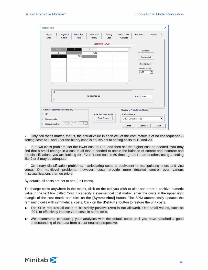
Salford Predictive Modeler® Introduction to Model Restoration
61
✓ Only cell ratios matter, that is, the actual value in each cell of the cost matrix is of no consequence—setting costs to 1 and 2 for the binary case is equivalent to setting costs to 10 and 20.
✓ In a two-class problem, set the lower cost to 1.00 and then set the higher cost as needed. You may find that a small change in a cost is all that is needed to obtain the balance of correct and incorrect and the classifications you are looking for. Even if one cost is 50 times greater than another, using a setting like 2 or 3 may be adequate.
✓ On binary classification problems, manipulating costs is equivalent to manipulating priors and vice versa. On multilevel problems, however, costs provide more detailed control over various misclassifications than do priors.
By default, all costs are set to one (unit costs).
To change costs anywhere in the matrix, click on the cell you wish to alter and enter a positive numeric
value in the text box called Cost. To specify a symmetrical cost matrix, enter the costs in the upper right
triangle of the cost matrix and click on the [Symmetrical] button. The SPM automatically updates the
remaining cells with symmetrical costs. Click on the [Defaults] button to restore the unit costs.
The SPM requires all costs to be strictly positive (zero is not allowed). Use small values, such as .001, to effectively impose zero costs in some cells.
We recommend conducting your analyses with the default costs until you have acquired a good understanding of the data from a cost-neutral perspective.

Salford Predictive Modeler® Introduction to Model Restoration
62
Priors tab
✓ This is a classification-only feature.
PRIORS EQUAL
PRIORS DATA
PRIORS MIX
PRIORS LEARN
PRIORS TEST
PRIORS SPECIFY <class1>=<value1>, <class2>=<value2>, ...
The Model Setup—Priors tab is one of the most important options you can set in shaping a classification
analysis and you need to understand the basics of it to get the most out of the SPM. Although the
PRIORS terminology is unfamiliar to most analysts, the core concepts are relatively easy to grasp. Market
researchers and biomedical analysts make use of the priors concepts routinely but in the context of a
different vocabulary.
We start by discussing a straightforward 0/1 or YES/NO classification problem. In most real world
situations, the YES or 1 group is relatively rare. For example, in a large field of prospects only a few
become customers, relatively few borrowers default on their loans, only a tiny fraction of credit card
transactions and insurance claims are fraudulent, etc. The relative rarity of a class in the real world is
usually reflected in the data available for analysis. A file containing data on 100,000 borrowers might
include no more than 4,000 bankrupts for a mainstream lender.
Such unbalanced data sets are quite natural for SPM and pose no special problems for analysis. This is
one of SPM’s great strengths and differentiates SPM from other analytical tools that do not perform well
unless the data are “balanced”.
The SPM default method for dealing with unbalanced data is to conduct all analyses using measures that
are relative to each class. In our example of 100,000 records containing 4,000 bankrupts, we will always
work with ratios that are computed relative to 4,000 for the bankrupts and relative to 96,000 for the non-
bankrupts. By doing everything in relative terms we bypass completely the fact that one of the two groups
is 24 times the size of the other.
This method of bookkeeping is known as PRIORS EQUAL. It is the default method used for classification
models and it often works supremely well. This is the setting we almost always use to start our exploration
of new data. This default setting frequently gives the most satisfactory results because each class is
treated as equally important for the purpose of achieving classification accuracy.
Priors are usually specified as fractions that sum to 1.0. In a two-class problem EQUAL priors would be
expressed numerically as 0.50, 0.50, and in a three-class problem they would be expressed as 0.333,
0.333, 0.333.
PRIORS may look like weights but they are not weights. Priors reflect the relative size of a class after SPM has made its adjustments. Thus, PRIORS EQUAL assures that no matter how small a class may be relative to the other classes, it will be treated as if it were of equal size.
PRIORS DATA (or PRIORS LEARN or PRIORS TEST) makes no adjustments for relative class sizes. Under this setting small classes will have less influence on the SPM tree and may even be ignored if they interfere with the SPM’s ability to classify the larger classes accurately.
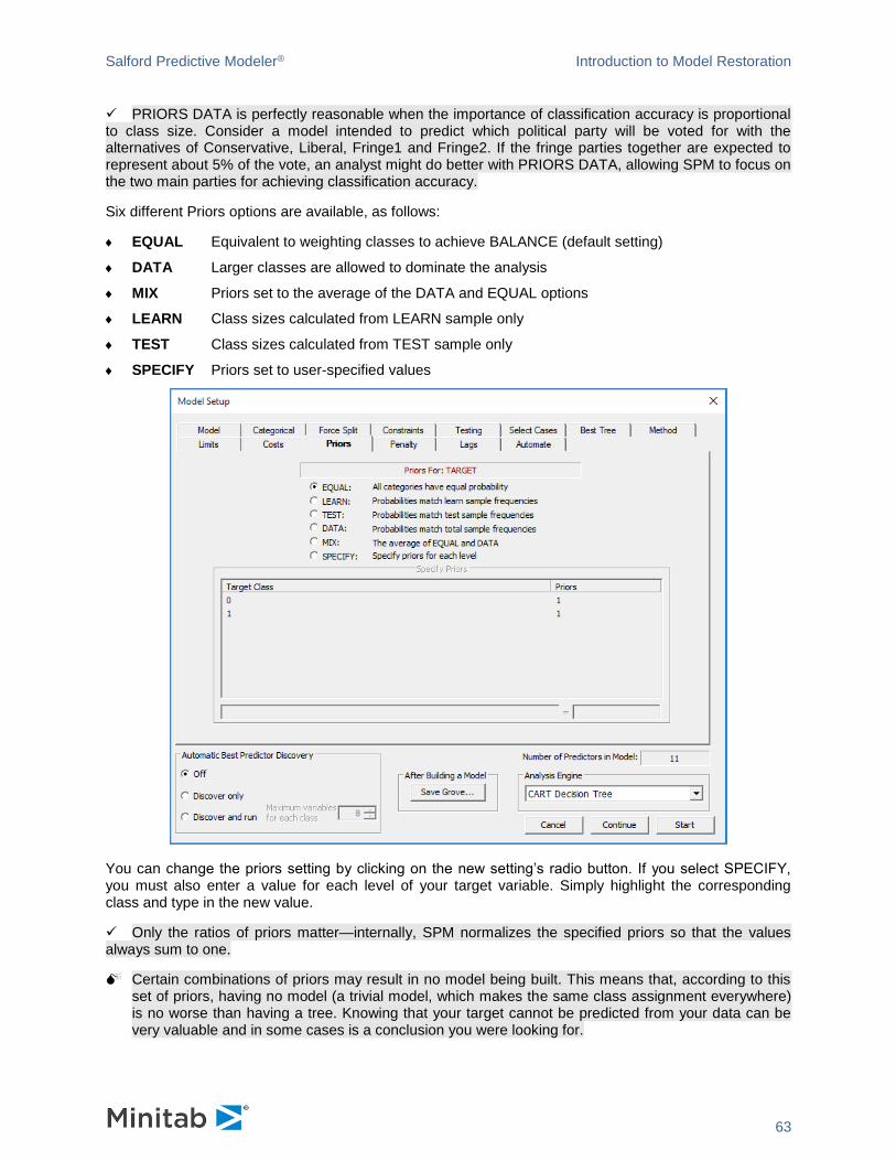
Salford Predictive Modeler® Introduction to Model Restoration
63
✓ PRIORS DATA is perfectly reasonable when the importance of classification accuracy is proportional to class size. Consider a model intended to predict which political party will be voted for with the alternatives of Conservative, Liberal, Fringe1 and Fringe2. If the fringe parties together are expected to represent about 5% of the vote, an analyst might do better with PRIORS DATA, allowing SPM to focus on the two main parties for achieving classification accuracy.
Six different Priors options are available, as follows:
EQUAL Equivalent to weighting classes to achieve BALANCE (default setting)
DATA Larger classes are allowed to dominate the analysis
MIX Priors set to the average of the DATA and EQUAL options
LEARN Class sizes calculated from LEARN sample only
TEST Class sizes calculated from TEST sample only
SPECIFY Priors set to user-specified values
You can change the priors setting by clicking on the new setting’s radio button. If you select SPECIFY, you must also enter a value for each level of your target variable. Simply highlight the corresponding class and type in the new value.
✓ Only the ratios of priors matter—internally, SPM normalizes the specified priors so that the values always sum to one.
Certain combinations of priors may result in no model being built. This means that, according to this set of priors, having no model (a trivial model, which makes the same class assignment everywhere) is no worse than having a tree. Knowing that your target cannot be predicted from your data can be very valuable and in some cases is a conclusion you were looking for.

Salford Predictive Modeler® Introduction to Model Restoration
64
If the target variable contains >5000 values, you must use the Command Language for user-specified priors.
Penalty tab
✓ This section uses CART® to demonstrate how penalties work, but they are available for other Analysis Engines too.
PENALTY <var>=<penalty>, /MISSING=<mis_val1>,<mis_val2>,
HLC=<hlc_val1>,<hlc_val2>
PENALTY /MISSING=1,1, HLC=1,1
The penalties available in SPM were introduced by Salford Systems starting in 1997 and represent
important extensions to machine learning technology. Penalties can be imposed on variables to reflect a
reluctance to use a variable as a predictor. Of course, the modeler can always exclude a variable; the
penalty offers an opportunity to permit a variable into the model but only under special circumstances.
The three categories of penalty are:
Missing Value Penalty: Predictors are penalized to reflect how frequently they are missing. The penalty is recalculated for every node in the tree.
High Level Categorical Penalty: Categorical predictors with many levels can distort a tree due to their explosive splitting power. The HLC penalty levels the playing field.
Predictor Specific Penalties: Each predictor can be assigned a custom penalty.
In CART®, a penalty will lower a predictor’s improvement score, thus making it less likely to be chosen as
the primary splitter. Penalties specific to particular predictors are entered in the left panel next to the
predictor name and may range from zero to one inclusive.
Penalties for missing values (for categorical and continuous predictors) and a high number of levels (for categorical predictors only) can range from "No Penalty" to "High Penalty" and are normally set via the slider on the Penalty tab, as seen in the following illustration.
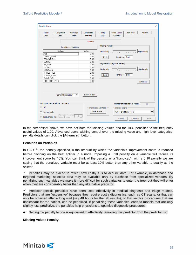
Salford Predictive Modeler® Introduction to Model Restoration
65
In the screenshot above, we have set both the Missing Values and the HLC penalties to the frequently useful values of 1.00. Advanced users wishing control over the missing value and high-level categorical penalty details can click the [Advanced] button.
Penalties on Variables
In CART®, the penalty specified is the amount by which the variable’s improvement score is reduced
before deciding on the best splitter in a node. Imposing a 0.10 penalty on a variable will reduce its
improvement score by 10%. You can think of the penalty as a “handicap”: with a 0.10 penalty we are
saying that the penalized variable must be at least 10% better than any other variable to qualify as the
splitter.
✓ Penalties may be placed to reflect how costly it is to acquire data. For example, in database and targeted marketing, selected data may be available only by purchase from specialized vendors. By penalizing such variables we make it more difficult for such variables to enter the tree, but they will enter when they are considerably better than any alternative predictor.
✓ Predictor-specific penalties have been used effectively in medical diagnosis and triage models. Predictors that are “expensive” because they require costly diagnostics, such as CT scans, or that can only be obtained after a long wait (say 48 hours for the lab results), or that involve procedures that are unpleasant for the patient, can be penalized. If penalizing these variables leads to models that are only slightly less predictive, the penalties help physicians to optimize diagnostic procedures.
Setting the penalty to one is equivalent to effectively removing this predictor from the predictor list.
Missing Values Penalty
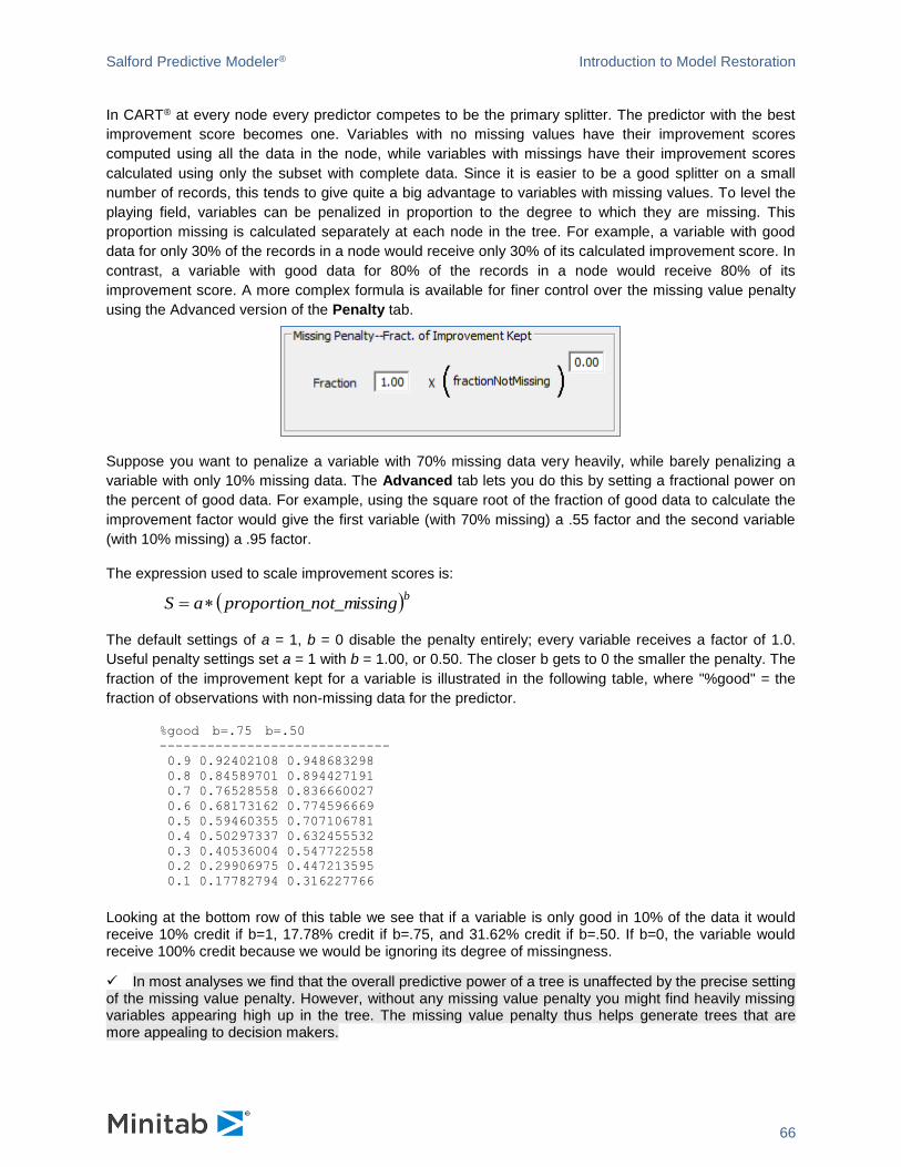
Salford Predictive Modeler® Introduction to Model Restoration
66
In CART® at every node every predictor competes to be the primary splitter. The predictor with the best
improvement score becomes one. Variables with no missing values have their improvement scores
computed using all the data in the node, while variables with missings have their improvement scores
calculated using only the subset with complete data. Since it is easier to be a good splitter on a small
number of records, this tends to give quite a big advantage to variables with missing values. To level the
playing field, variables can be penalized in proportion to the degree to which they are missing. This
proportion missing is calculated separately at each node in the tree. For example, a variable with good
data for only 30% of the records in a node would receive only 30% of its calculated improvement score. In
contrast, a variable with good data for 80% of the records in a node would receive 80% of its
improvement score. A more complex formula is available for finer control over the missing value penalty
using the Advanced version of the Penalty tab.
Suppose you want to penalize a variable with 70% missing data very heavily, while barely penalizing a
variable with only 10% missing data. The Advanced tab lets you do this by setting a fractional power on
the percent of good data. For example, using the square root of the fraction of good data to calculate the
improvement factor would give the first variable (with 70% missing) a .55 factor and the second variable
(with 10% missing) a .95 factor.
The expression used to scale improvement scores is:
The default settings of a = 1, b = 0 disable the penalty entirely; every variable receives a factor of 1.0.
Useful penalty settings set a = 1 with b = 1.00, or 0.50. The closer b gets to 0 the smaller the penalty. The
fraction of the improvement kept for a variable is illustrated in the following table, where "%good" = the
fraction of observations with non-missing data for the predictor.
%good b=.75 b=.50
-----------------------------
0.9 0.92402108 0.948683298
0.8 0.84589701 0.894427191
0.7 0.76528558 0.836660027
0.6 0.68173162 0.774596669
0.5 0.59460355 0.707106781
0.4 0.50297337 0.632455532
0.3 0.40536004 0.547722558
0.2 0.29906975 0.447213595
0.1 0.17782794 0.316227766
Looking at the bottom row of this table we see that if a variable is only good in 10% of the data it would receive 10% credit if b=1, 17.78% credit if b=.75, and 31.62% credit if b=.50. If b=0, the variable would receive 100% credit because we would be ignoring its degree of missingness.
✓ In most analyses we find that the overall predictive power of a tree is unaffected by the precise setting of the missing value penalty. However, without any missing value penalty you might find heavily missing variables appearing high up in the tree. The missing value penalty thus helps generate trees that are more appealing to decision makers.
( )bng_not_missiproportionaS =

Salford Predictive Modeler® Introduction to Model Restoration
67
High-Level Categorical Penalty
Categorical predictors present a special challenge to decision trees. Because a 32-level categorical
predictor can split a data set in over two billion ways, even a totally random variable has a high probability
of becoming the primary splitter in many nodes. Such spurious splits will not prevent the SPM from
eventually detecting the true data structure in large datasets, but they make the process inefficient. First,
they add unwanted nodes to a tree, and as they promote the fragmentation of the data into added nodes,
the reduced sample size as we progress down the tree makes it harder to find the best splits.
To protect against this possibility, SPM offers a high-level categorical predictor penalty used to reduce the
measured splitting power. On the Basic Penalty dialog, this is controlled with a simple slider.
The Advanced Penalty dialog allows access to the full penalty expression. The improvement factor is
expressed as:
By default, c = 1 and d = 0; these values disable the penalty. We recommend that the categorical variable
penalty be set to (c = 1, d = 1), which ensures that a categorical predictor has no inherent advantage over
a continuous variable with unique values for every record.
The missing value and HLC penalties apply uniformly for all variables. You cannot set different HLC or missing value penalties to different variables. You choose one setting for each penalty and it will apply to all variables.
✓ You can set variable-specific penalties and general missing value and HLC penalties. Thus, if you have a categorical variable Z that is also sometimes missing you could have all three penalties applying to this variable at the same time.
−+= −1
1_
_log1,1min 2
d
categoriesN
sizenodecS
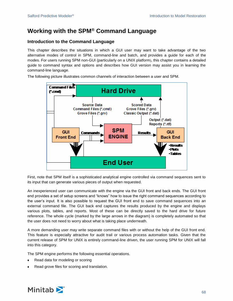
Salford Predictive Modeler® Introduction to Model Restoration
68
Working with the SPM® Command Language
Introduction to the Command Language
This chapter describes the situations in which a GUI user may want to take advantage of the two
alternative modes of control in SPM, command-line and batch, and provides a guide for each of the
modes. For users running SPM non-GUI (particularly on a UNIX platform), this chapter contains a detailed
guide to command syntax and options and describes how GUI version may assist you in learning the
command-line language.
The following picture illustrates common channels of interaction between a user and SPM.
First, note that SPM itself is a sophisticated analytical engine controlled via command sequences sent to
its input that can generate various pieces of output when requested.
An inexperienced user can communicate with the engine via the GUI front and back ends. The GUI front
end provides a set of setup screens and “knows” how to issue the right command sequences according to
the user’s input. It is also possible to request the GUI front end to save command sequences into an
external command file. The GUI back end captures the results produced by the engine and displays
various plots, tables, and reports. Most of these can be directly saved to the hard drive for future
reference. The whole cycle (marked by the large arrows in the diagram) is completely automated so that
the user does not need to worry about what is taking place underneath.
A more demanding user may write separate command files with or without the help of the GUI front end.
This feature is especially attractive for audit trail or various process automation tasks. Given that the
current release of SPM for UNIX is entirely command-line driven, the user running SPM for UNIX will fall
into this category.
The SPM engine performs the following essential operations.
Read data for modeling or scoring
Read grove files for scoring and translation.
Salford Predictive Modeler® Introduction to Model Restoration
69
Read and executes command files.
Write new data composed of original data and scoring information.
Save models into grove files.
Save classic text output.
The following sections provide in-depth discussions for users who have chosen to use command line controls.
Alternative Control Modes in SPM® for Windows
In addition to controlling SPM with the graphical user interface (GUI), you can control the program via
commands issued at the command prompt or via submission of a command (.cmd) file. This built-in
flexibility enables you to avoid repetition, create an audit trail, and take advantage of the BASIC
programming language.
Avoiding Repetition
You may need to interact with several dialogs to define your model and set model estimation options.
This is particularly true when a model has a large number of variables or many categorical variables, or
when more than just a few options must be set to build the desired model. Suppose that a series of runs
are to be accomplished, with little variation between each. A batch command file, containing the
commands that define the basic model and options, provides an easy way to perform many SPM
command functions in one user step. For each run in the series, the “core” batch command file can be
submitted to SPM, followed by the few graphical user interface selections necessary for the particular run
in question.
Creating an Audit Trail
The Command Log window can help you create an audit trail when one is needed. Imagine not being
able to reproduce a particular analysis track, perhaps because the specific set of options used to create a
model (e.g., the name of the data set itself) was never recorded. The updated command log provides you
with the entire command set necessary to exactly reproduce your analysis, provided the input data do not
change.
Taking Advantage of SPM’s Built-In Programming Language
SPM offers an integrated BASIC programming language that allows the user to define new variables,
modify existing variables, access mathematical, statistical and probability distribution functions, and
define flexible criteria to control case deletion and the partitioning of data into learn and test samples.
Small BASIC programs are defined near the beginning of your analysis session, after you have opened
your dataset but before you estimate (or apply) the model and usually before defining the list of predictor
variables. BASIC is powerful enough that in many cases users do not need to resort to a stand-alone data
manipulation program.
Open a Notepad
Notepad window facilitates both creating and executing the scripts or Command Files. To create a new
Command File you can
Create New Notepad from main menu.
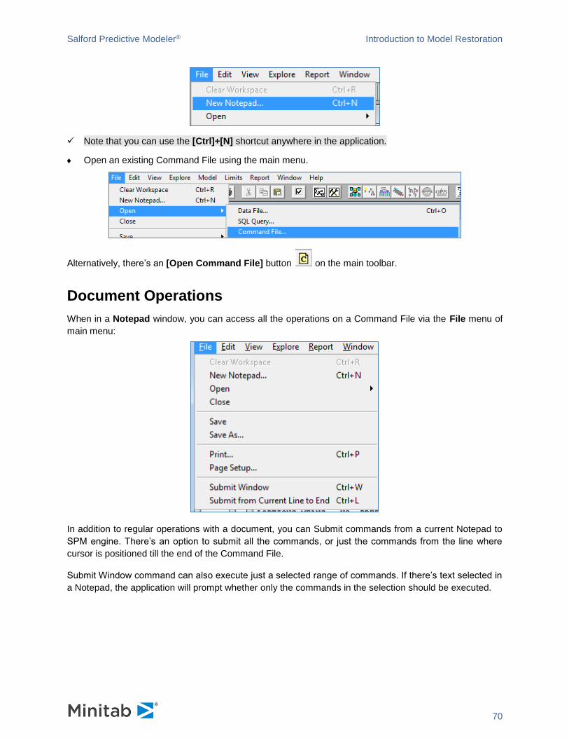
Salford Predictive Modeler® Introduction to Model Restoration
70
✓ Note that you can use the [Ctrl]+[N] shortcut anywhere in the application.
Open an existing Command File using the main menu.
Alternatively, there’s an [Open Command File] button on the main toolbar.
Document Operations
When in a Notepad window, you can access all the operations on a Command File via the File menu of
main menu:
In addition to regular operations with a document, you can Submit commands from a current Notepad to
SPM engine. There’s an option to submit all the commands, or just the commands from the line where
cursor is positioned till the end of the Command File.
Submit Window command can also execute just a selected range of commands. If there’s text selected in
a Notepad, the application will prompt whether only the commands in the selection should be executed.
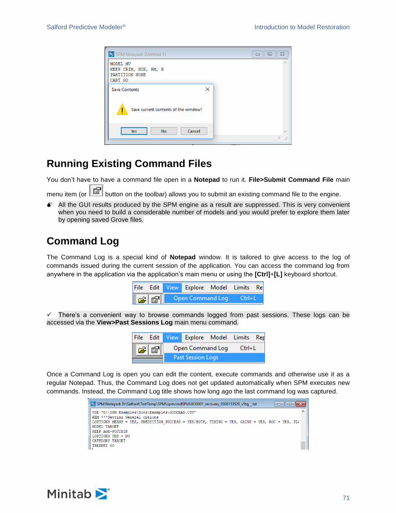
Salford Predictive Modeler® Introduction to Model Restoration
71
Running Existing Command Files
You don’t have to have a command file open in a Notepad to run it. File>Submit Command File main
menu item (or button on the toolbar) allows you to submit an existing command file to the engine.
All the GUI results produced by the SPM engine as a result are suppressed. This is very convenient when you need to build a considerable number of models and you would prefer to explore them later by opening saved Grove files.
Command Log
The Command Log is a special kind of Notepad window. It is tailored to give access to the log of
commands issued during the current session of the application. You can access the command log from
anywhere in the application via the application’s main menu or using the [Ctrl]+[L] keyboard shortcut.
✓ There’s a convenient way to browse commands logged from past sessions. These logs can be accessed via the View>Past Sessions Log main menu command.
Once a Command Log is open you can edit the content, execute commands and otherwise use it as a
regular Notepad. Thus, the Command Log does not get updated automatically when SPM executes new
commands. Instead, the Command Log title shows how long ago the last command log was captured.

Salford Predictive Modeler® Introduction to Model Restoration
72
To refresh the Command Log, [Right-Click] anywhere in the Command Log window and select Update
Command Log menu item:
All the modifications to the Command Log window will be lost during the update. To preserve the edits they must be copied to a regular Notepad window.
✓ This feature is helpful for learning command syntax.
✓ You may save the Command Log into a command file on your hard drive using the File>Save menu. CART® session, the resulting command file will contain the audit trail of the entire session.
Authoring Command Files
One of the common scenarios to author a command file is to take a Command Log and extract the
relevant commands. This way you can reproduce the analysis you did at any time in the future. This is
also a good starting point to acquire practical understanding of the SPM Command Language. Even most
experienced users in many cases prefer using the Model Setup window to prepare a sketch of the
command file and then take generated command log as a basis for the script.
When working with a script, the Command Builder window comes in handy to lookup command syntax,
variables available in the current dataset, and code snippets for typical tasks.
The Command Builder window can be turned ON and OFF via View menu item of the main menu.
Command Builder content structure
Lookup information in the Command Builder is organized into 3 major sections.
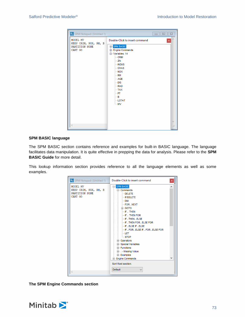
Salford Predictive Modeler® Introduction to Model Restoration
73
SPM BASIC language
The SPM BASIC section contains reference and examples for built-in BASIC language. The language
facilitates data manipulation. It is quite effective in prepping the data for analysis. Please refer to the SPM
BASIC Guide for more detail.
This lookup information section provides reference to all the language elements as well as some
examples.
The SPM Engine Commands section
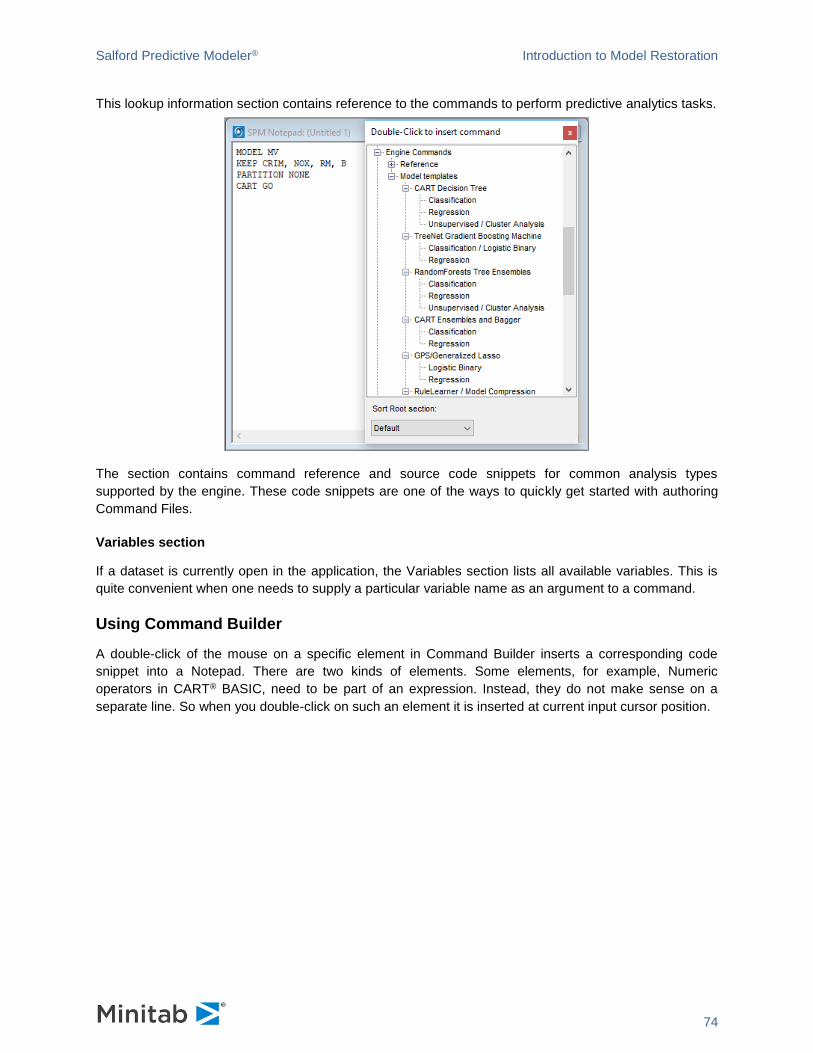
Salford Predictive Modeler® Introduction to Model Restoration
74
This lookup information section contains reference to the commands to perform predictive analytics tasks.
The section contains command reference and source code snippets for common analysis types
supported by the engine. These code snippets are one of the ways to quickly get started with authoring
Command Files.
Variables section
If a dataset is currently open in the application, the Variables section lists all available variables. This is
quite convenient when one needs to supply a particular variable name as an argument to a command.
Using Command Builder
A double-click of the mouse on a specific element in Command Builder inserts a corresponding code
snippet into a Notepad. There are two kinds of elements. Some elements, for example, Numeric
operators in CART® BASIC, need to be part of an expression. Instead, they do not make sense on a
separate line. So when you double-click on such an element it is inserted at current input cursor position.
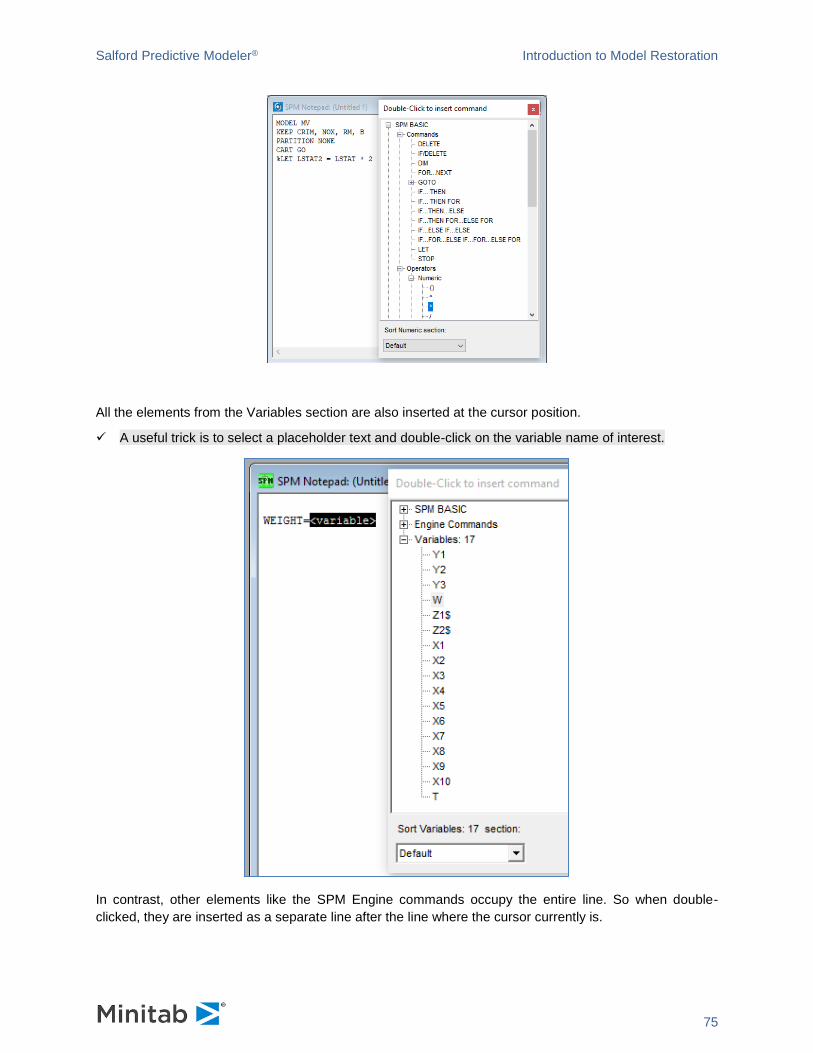
Salford Predictive Modeler® Introduction to Model Restoration
75
All the elements from the Variables section are also inserted at the cursor position.
✓ A useful trick is to select a placeholder text and double-click on the variable name of interest.
In contrast, other elements like the SPM Engine commands occupy the entire line. So when double-
clicked, they are inserted as a separate line after the line where the cursor currently is.
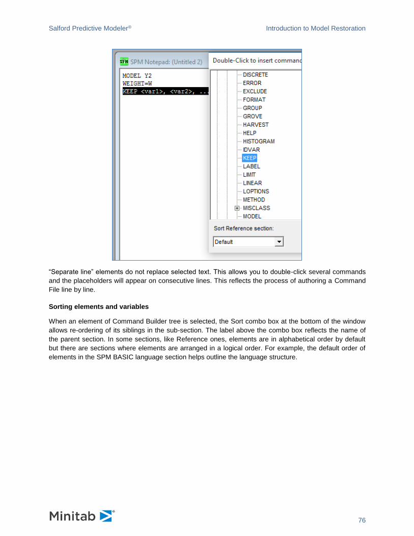
Salford Predictive Modeler® Introduction to Model Restoration
76
“Separate line” elements do not replace selected text. This allows you to double-click several commands
and the placeholders will appear on consecutive lines. This reflects the process of authoring a Command
File line by line.
Sorting elements and variables
When an element of Command Builder tree is selected, the Sort combo box at the bottom of the window
allows re-ordering of its siblings in the sub-section. The label above the combo box reflects the name of
the parent section. In some sections, like Reference ones, elements are in alphabetical order by default
but there are sections where elements are arranged in a logical order. For example, the default order of
elements in the SPM BASIC language section helps outline the language structure.
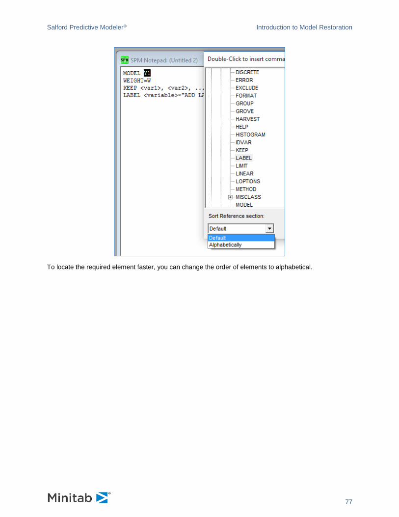
Salford Predictive Modeler® Introduction to Model Restoration
77
To locate the required element faster, you can change the order of elements to alphabetical.
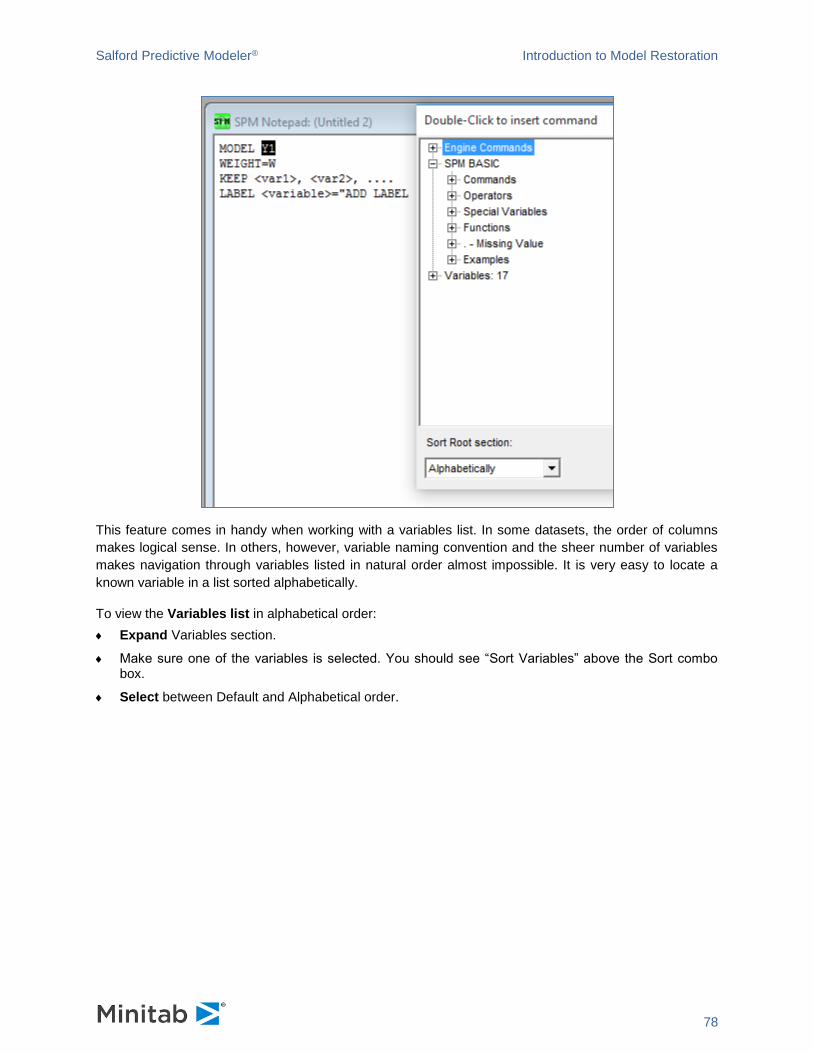
Salford Predictive Modeler® Introduction to Model Restoration
78
This feature comes in handy when working with a variables list. In some datasets, the order of columns
makes logical sense. In others, however, variable naming convention and the sheer number of variables
makes navigation through variables listed in natural order almost impossible. It is very easy to locate a
known variable in a list sorted alphabetically.
To view the Variables list in alphabetical order:
Expand Variables section.
Make sure one of the variables is selected. You should see “Sort Variables” above the Sort combo box.
Select between Default and Alphabetical order.
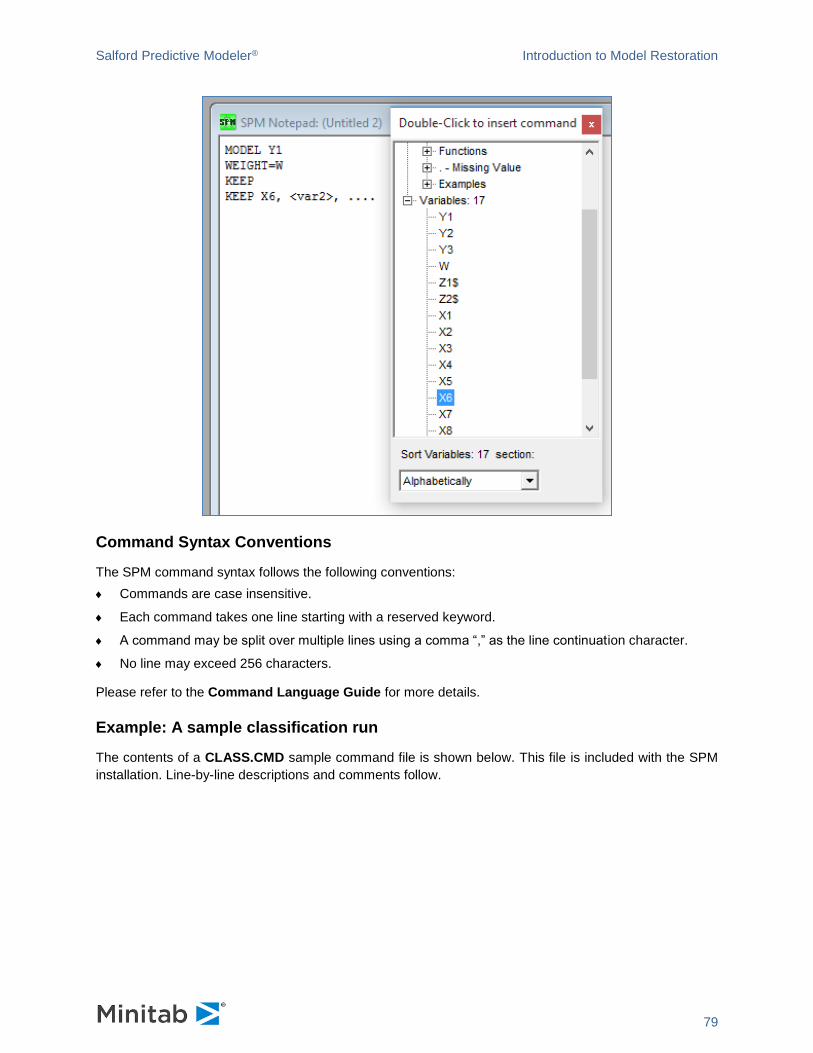
Salford Predictive Modeler® Introduction to Model Restoration
79
Command Syntax Conventions
The SPM command syntax follows the following conventions:
Commands are case insensitive.
Each command takes one line starting with a reserved keyword.
A command may be split over multiple lines using a comma “,” as the line continuation character.
No line may exceed 256 characters.
Please refer to the Command Language Guide for more details.
Example: A sample classification run
The contents of a CLASS.CMD sample command file is shown below. This file is included with the SPM
installation. Line-by-line descriptions and comments follow.
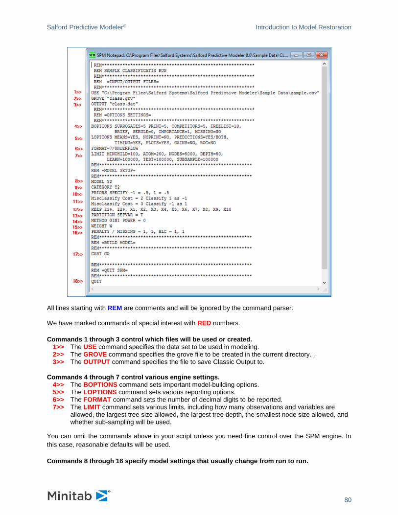
Salford Predictive Modeler® Introduction to Model Restoration
80
All lines starting with REM are comments and will be ignored by the command parser.
We have marked commands of special interest with RED numbers.
Commands 1 through 3 control which files will be used or created. 1>> The USE command specifies the data set to be used in modeling. 2>> The GROVE command specifies the grove file to be created in the current directory. . 3>> The OUTPUT command specifies the file to save Classic Output to.
Commands 4 through 7 control various engine settings. 4>> The BOPTIONS command sets important model-building options. 5>> The LOPTIONS command sets various reporting options. 6>> The FORMAT command sets the number of decimal digits to be reported. 7>> The LIMIT command sets various limits, including how many observations and variables are
allowed, the largest tree size allowed, the largest tree depth, the smallest node size allowed, and whether sub-sampling will be used.
You can omit the commands above in your script unless you need fine control over the SPM engine. In
this case, reasonable defaults will be used.
Commands 8 through 16 specify model settings that usually change from run to run.

Salford Predictive Modeler® Introduction to Model Restoration
81
8>> The MODEL command sets the target variable. 9>> The CATEGORY command lists all categorical numeric variables.
✓ Character variables are always treated as categorical and need not be listed here.
✓ For classification models, numeric targets must be declared categorical.
10>> The PRIORS command sets the prior probabilities for all target classes.
The commands PRIORS DATA or PRIORS EQUAL are useful aliases for common situations. 11>> The MISCLASSIFY commands set the cost matrix.
✓ Only non-unit costs need to be introduced explicitly.
✓ There will be as many MISCLASSIFY commands as there are non-unit cost cells in the cost matrix.
12>> The KEEP command sets the predictor list.
This command is NOT cumulative.
13>> The PARTITION command specifies the LEARN/TEST partition method.
✓ In this example, a dummy variable T separates the TEST part (T=1) from the LEARN part (T=0).
14>> The METHOD command sets the improvement calculation method.
✓ The commands METHOD GINI and METHOD TWOING are the most widely-used methods.
✓ POWER>0 results in more even splits.
15>> The WEIGHT command sets the weight variable, if applicable. 16>> The PENALTY command induces additional penalties on missing-value and high-level
categorical predictors.
✓ We recommend always using the listed penalties.
The remaining two commands are “action” commands. 17>> The BUILD command signals the SPM engine to start the model-building process. 18>> The QUIT command terminates the program.
Anything following QUIT in the command file will be ignored.
Multiple runs may be conducted using a single command file by inserting additional commands.
Example: A sample regression run
The contents of a REG.CMD (or REGRESS.CMD) sample command file are shown below. This file is included with the SPM installation. Line-by-line descriptions and comments follow.
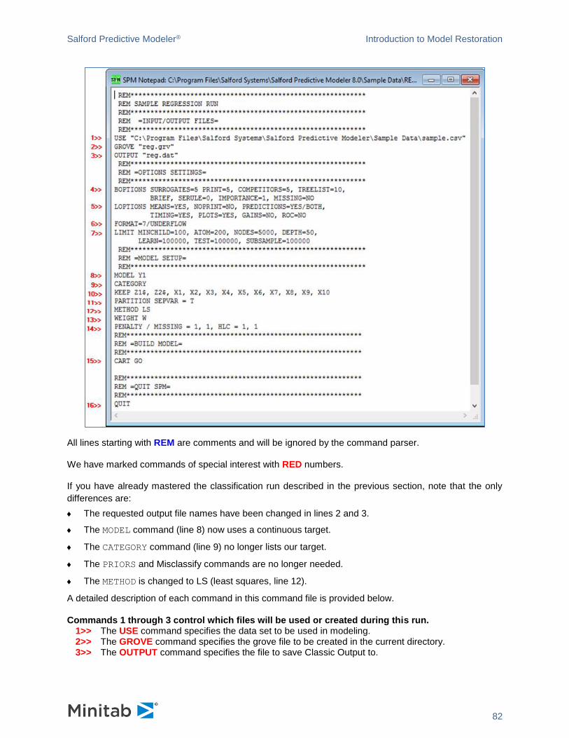
Salford Predictive Modeler® Introduction to Model Restoration
82
All lines starting with REM are comments and will be ignored by the command parser.
We have marked commands of special interest with RED numbers.
If you have already mastered the classification run described in the previous section, note that the only
differences are:
The requested output file names have been changed in lines 2 and 3.
The MODEL command (line 8) now uses a continuous target.
The CATEGORY command (line 9) no longer lists our target.
The PRIORS and Misclassify commands are no longer needed.
The METHOD is changed to LS (least squares, line 12).
A detailed description of each command in this command file is provided below.
Commands 1 through 3 control which files will be used or created during this run. 1>> The USE command specifies the data set to be used in modeling. 2>> The GROVE command specifies the grove file to be created in the current directory. 3>> The OUTPUT command specifies the file to save Classic Output to.

Salford Predictive Modeler® Introduction to Model Restoration
83
Commands 4 through 7 control various engine settings. 4>> The BOPTIONS command sets important model-building options. 5>> The LOPTIONS command sets various reporting options. 6>> The FORMAT command sets the number of decimal digits to be reported. 7>> The LIMIT command sets various limits, including how many how many observations and
variables are allowed are allowed, the largest tree size allowed, the largest tree depth, the smallest node size allowed, and whether sub-sampling will be used.
For the most part, these commands should be left unchanged unless you need fine control over the SPM
engine. A more detailed description can be found in the Appendix III Command Reference.
Commands 8 through 16 specify model settings that usually change from run to run. 8>> The MODEL command sets the target variable. 9>> The CATEGORY command lists all categorical numeric variables.
✓ Character variables are always treated as categorical and need not be listed here.
✓ In regression runs, the target is always a continuous numeric variable.
10>> The KEEP command sets the predictor list.
This command is NOT cumulative.
11>> The PARTITION command specifies the LEARN/TEST partition method.
✓ In this example, a dummy variable T separates the TEST part (T=1) from the LEARN part (T=0).
12>> The METHOD command sets the loss function.
✓ For regression CART® models, LS is least squares loss and LAD is least absolute deviation loss.
13>> The WEIGHT command sets the weight variable if applicable. 14>> The PENALTY command induces additional penalties on missing-value and high-level
categorical predictors.
✓ We recommend always using the listed penalties.
The remaining two commands are “action” commands. 15>> The BUILD command signals the SPM engine to start the model-building process. 16>> The QUIT command terminates the program.
✓ Anything following QUIT in the command file will be ignored.
Multiple runs may be conducted using a single command file by inserting additional commands.
Example: A sample scoring run
The contents of a SCORE.CMD sample command file are shown below. This file is included with the SPM
installation. Line-by-line descriptions and comments follow.
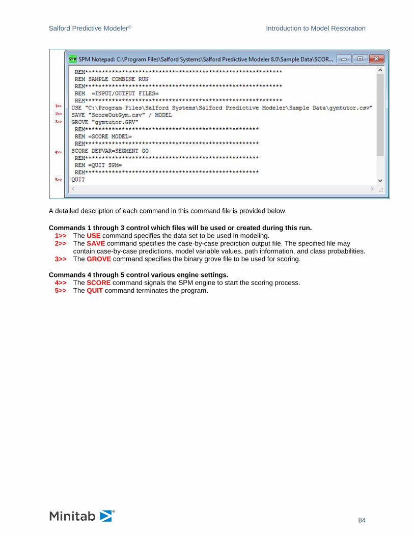
Salford Predictive Modeler® Introduction to Model Restoration
84
A detailed description of each command in this command file is provided below.
Commands 1 through 3 control which files will be used or created during this run. 1>> The USE command specifies the data set to be used in modeling. 2>> The SAVE command specifies the case-by-case prediction output file. The specified file may
contain case-by-case predictions, model variable values, path information, and class probabilities. 3>> The GROVE command specifies the binary grove file to be used for scoring.
Commands 4 through 5 control various engine settings. 4>> The SCORE command signals the SPM engine to start the scoring process. 5>> The QUIT command terminates the program.

Salford Predictive Modeler® Introduction to Model Restoration
85
Introduction to Model Restoration
This guide describes this new feature in SPM 8.0 used to save and restore the “state of the session”
allowing model restoration at a future point in time.
Introductory User Story:
Morgan has just spent the last two hours working with a data file containing 2,000 variables of which only
1,600 are to be selected as predictors. Some of the variables are categorical. Morgan experimented with
many different test methods, various selection methods, and experimented with defining control
parameters, options, and settings. Morgan is happy with resulting model based on the last two hours of
work.
Question:
How does Morgan save the work accumulated over the last two hours and return to this stopping point at
some later point in time? Morgan would also like to send the progress to colleagues who can use as a
starting point for further modeling.
Answer:
What Morgan needs is the ability to capture the state of the modeling session currently being worked with
into some type of file (container). The history of a session leading up to any given point in time results in
an "engine state" of the session, complete with hundreds of user parameters, options, and settings. This
file will contain an “engine state” and a “session state” which will be discussed later in the walk-about.
As a result, SPM introduces the functionality of “Model Restoration”. The concept of Model Restoration is
to use a file (container) to recall and restore Morgan’s modeling session. As a result, SPM enables
Morgan to return to a previous modeling session, allowing Morgan and his colleagues to pick up work
where they left off.
Given the user’s story above, this functionality can significantly reduce the manual burden on setting up
and running models in the graphical user interface. With 1,500 variables to select, automatically
identifying and selecting target, predictor, and categorical variables alone is a time saver. Considering all
other factors and activities that usually take place during the modeling cycle, various time savings that
may result from being able to restore engine and session settings becomes significant added value to the
modeler.
Getting Started with Model Restoration
The next stage of this walk-about is a guided tutorial through the detailed steps of setting up, creating,
and saving the modeling session file. This is followed by the saving of the model file (container), and
finally the recall and restore step.

Salford Predictive Modeler® Introduction to Model Restoration
86
Requirements and Approaches
What are the requirements and approaches for model restoration? The following is an outline of the
requirements which are discussed later in this document.
Grove Must be Created with SPM v8.3.
• While earlier versions of groves can still be used for scoring and model translation, this feature is not supported for grove files created in earlier versions of SPM.
Input Data File
• File name
• Variable names
• Variable ordering
• Variable count (more, less, etc.)
Model Restoration Tutorial
This tutorial will show you how to save and restore a SPM model. For this tutorial we will be building and
saving a simple binary TreeNet® model using the data file GOODBAD.CSV which is used in many
examples in this reference publication.
To open the input file GOODBAD.CSV:
Select Open>Data File… from the File menu.
✓ You may simply click on the button in the toolbar.
Use the Open Data File dialog window to navigate to the Sample Data folder in the SPM installation directory.
To speed up further access to the given location, you may want to set up the corresponding working directory first via Options dialog.
Choose Delimited (*.csv,*.dat,*.txt) in the Files of type: selection box.
Highlight GOODBAD.CSV.

Salford Predictive Modeler® Introduction to Model Restoration
87
Click the [Open] button to load the data set into TreeNet®.
Make sure that the data set is not currently being accessed by another application. If it is, the data loading will fail. This is a common source of problems when dealing with Excel and ASCII files.
In the resulting Activity window showing the basic info about the dataset, click the button
✓ The activity window step can be skipped using the Options dialog.
Setting up the Model
Controls are grouped into tabs in such a way that you need to visit only a minimal number of tabs to set up a SPM run. Simplest runs can be configured by only visiting the first Model tab.
In this tutorial we will visit only a selected set of these tabs to demonstrate some of the GUI controls
which can be saved and restored in the Model Restoration process.
Tab headings are displayed in RED when the tab requires information from you before a model can be
built. For example, when a dataset is open right after startup, the Model Setup dialog looks like this.
✓ Note: To ensure the ordering of variables match this guide, ensure you have select File Order for the Sort order.
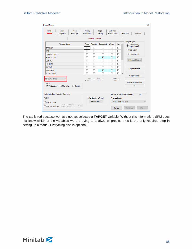
Salford Predictive Modeler® Introduction to Model Restoration
88
The tab is red because we have not yet selected a TARGET variable. Without this information, SPM does
not know which of the variables we are trying to analyze or predict. This is the only required step in
setting up a model. Everything else is optional.
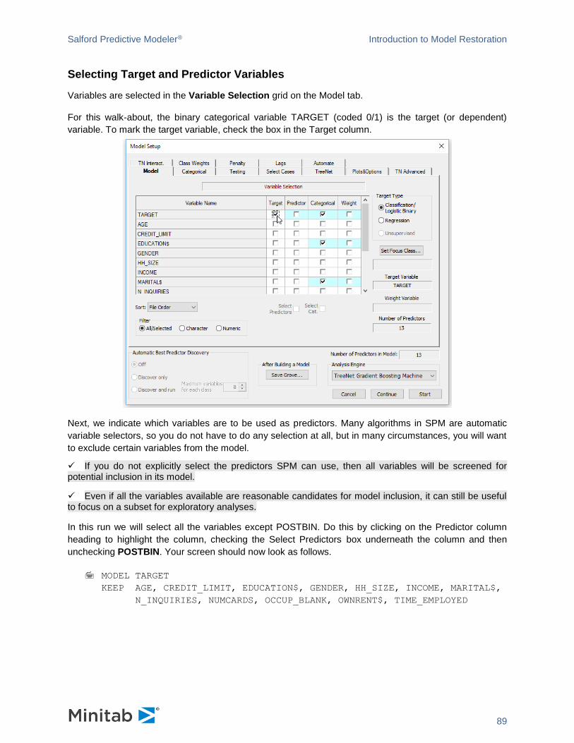
Salford Predictive Modeler® Introduction to Model Restoration
89
Selecting Target and Predictor Variables
Variables are selected in the Variable Selection grid on the Model tab.
For this walk-about, the binary categorical variable TARGET (coded 0/1) is the target (or dependent)
variable. To mark the target variable, check the box in the Target column.
Next, we indicate which variables are to be used as predictors. Many algorithms in SPM are automatic
variable selectors, so you do not have to do any selection at all, but in many circumstances, you will want
to exclude certain variables from the model.
✓ If you do not explicitly select the predictors SPM can use, then all variables will be screened for potential inclusion in its model.
✓ Even if all the variables available are reasonable candidates for model inclusion, it can still be useful to focus on a subset for exploratory analyses.
In this run we will select all the variables except POSTBIN. Do this by clicking on the Predictor column
heading to highlight the column, checking the Select Predictors box underneath the column and then
unchecking POSTBIN. Your screen should now look as follows.
MODEL TARGET
KEEP AGE, CREDIT_LIMIT, EDUCATION$, GENDER, HH_SIZE, INCOME, MARITAL$,
N_INQUIRIES, NUMCARDS, OCCUP_BLANK, OWNRENT$, TIME_EMPLOYED
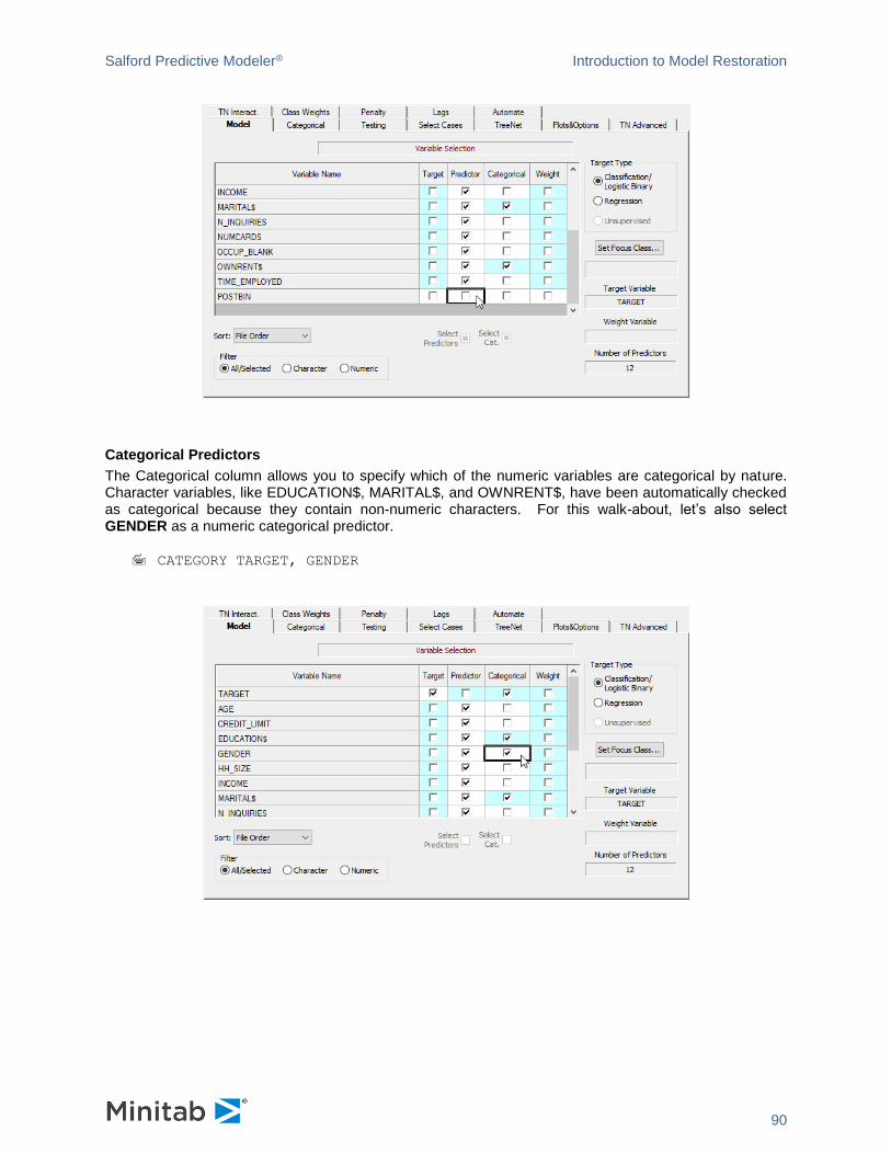
Salford Predictive Modeler® Introduction to Model Restoration
90
Categorical Predictors
The Categorical column allows you to specify which of the numeric variables are categorical by nature. Character variables, like EDUCATION$, MARITAL$, and OWNRENT$, have been automatically checked as categorical because they contain non-numeric characters. For this walk-about, let’s also select GENDER as a numeric categorical predictor.
CATEGORY TARGET, GENDER

Salford Predictive Modeler® Introduction to Model Restoration
91
Analysis Engine
This combo box allows you to select the Analysis Engine you would like to apply to the data. This walk-
about is focused on TreeNet® Gradient Boosting Machine
✓ The currently selected Analysis Engine determines which tabs are available. Also, the content of the tabs themselves could change according to the specifics of the Analysis Engine.
Choose the Classification/Logistic Binary radio button in the section labeled Target Type. In addition, be sure to select TreeNet Gradient Boosting Machine as the Analysis Engine.

Salford Predictive Modeler® Introduction to Model Restoration
92
Additional Model Setup Controls
Now that we have setup our Target and Predictor variables, let’s make some changes in additional tabs
which will demonstrate the value of Model Restoration. In this stage of the walk-about, we will visit the
following Model Setup dialog tabs making changes to various control parameters, options, and settings.
One of the objectives of Model Restoration that you will see is that all settings made in these next steps
will be preserved and become restorable for future use.
• Testing tab
• Select Cases tab
• TreeNet tab
• Plots & Options tab
• TN Interact tab
• Class Weights tab
• Penalty tab
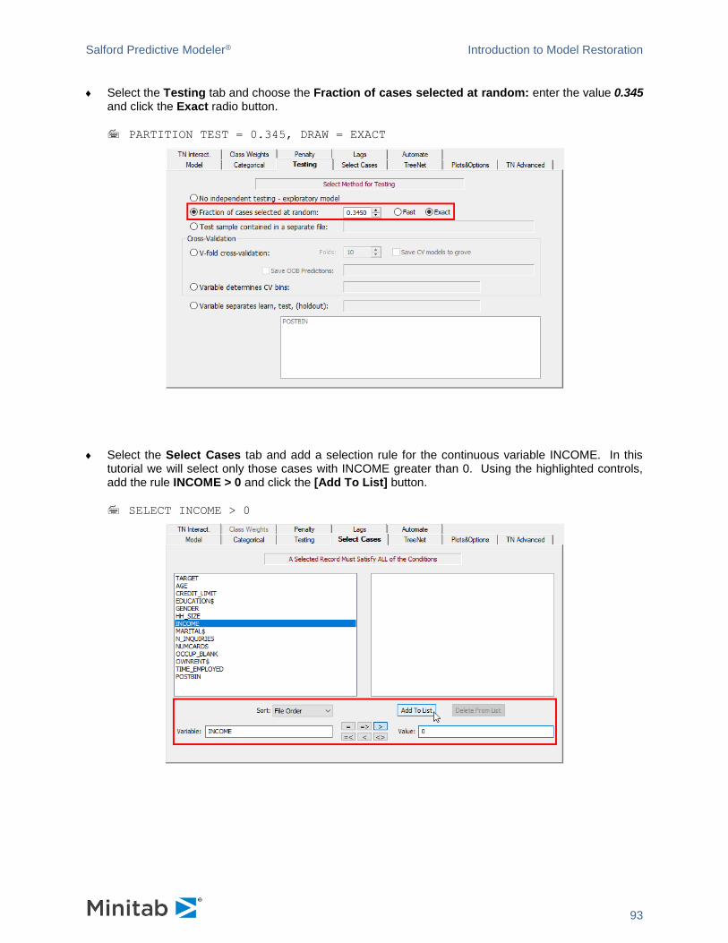
Salford Predictive Modeler® Introduction to Model Restoration
93
Select the Testing tab and choose the Fraction of cases selected at random: enter the value 0.345 and click the Exact radio button.
PARTITION TEST = 0.345, DRAW = EXACT
Select the Select Cases tab and add a selection rule for the continuous variable INCOME. In this tutorial we will select only those cases with INCOME greater than 0. Using the highlighted controls, add the rule INCOME > 0 and click the [Add To List] button.
SELECT INCOME > 0
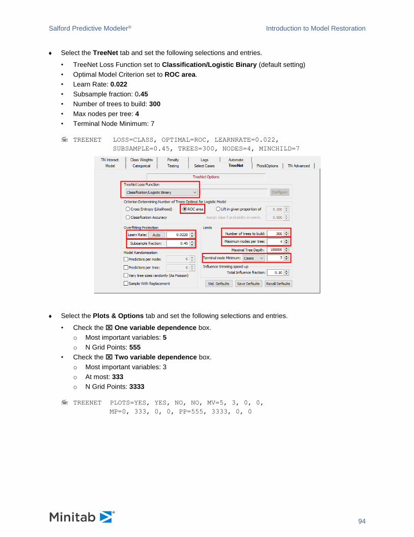
Salford Predictive Modeler® Introduction to Model Restoration
94
Select the TreeNet tab and set the following selections and entries.
• TreeNet Loss Function set to Classification/Logistic Binary (default setting)
• Optimal Model Criterion set to ROC area.
• Learn Rate: 0.022
• Subsample fraction: 0.45
• Number of trees to build: 300
• Max nodes per tree: 4
• Terminal Node Minimum: 7
TREENET LOSS=CLASS, OPTIMAL=ROC, LEARNRATE=0.022,
SUBSAMPLE=0.45, TREES=300, NODES=4, MINCHILD=7
Select the Plots & Options tab and set the following selections and entries.
• Check the One variable dependence box.
o Most important variables: 5
o N Grid Points: 555
• Check the Two variable dependence box.
o Most important variables: 3
o At most: 333
o N Grid Points: 3333
TREENET PLOTS=YES, YES, NO, NO, MV=5, 3, 0, 0,
MP=0, 333, 0, 0, PP=555, 3333, 0, 0
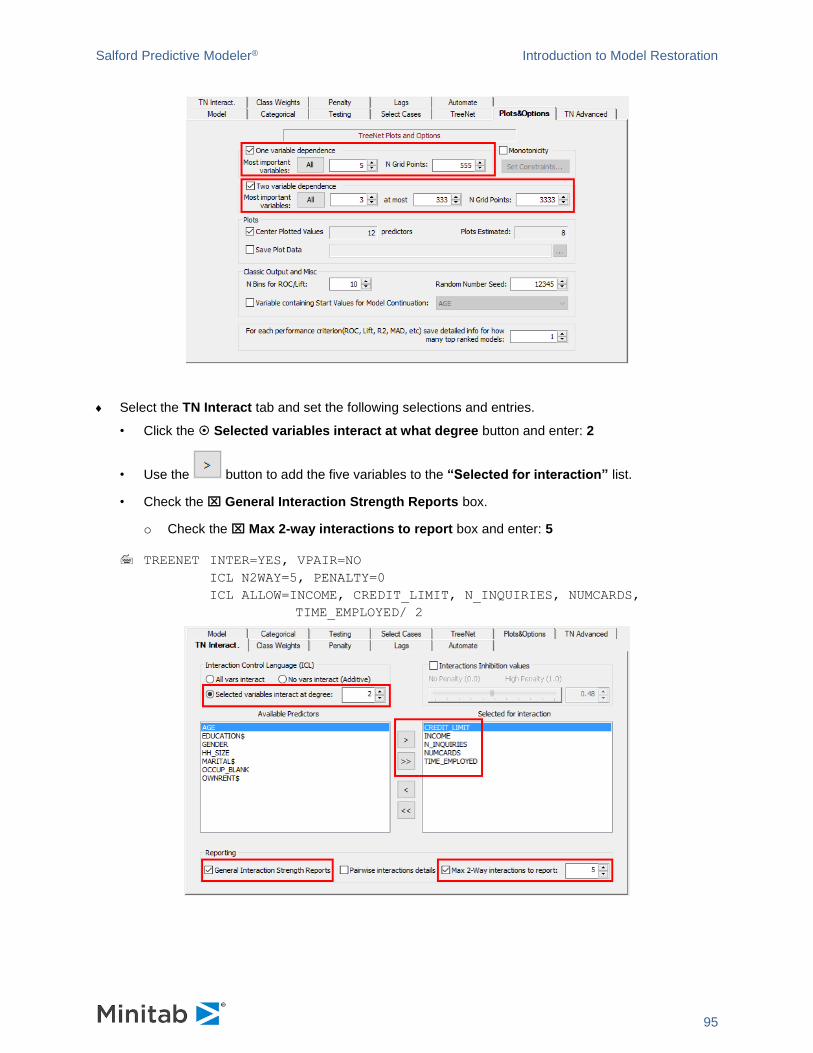
Salford Predictive Modeler® Introduction to Model Restoration
95
Select the TN Interact tab and set the following selections and entries.
• Click the Selected variables interact at what degree button and enter: 2
• Use the button to add the five variables to the “Selected for interaction” list.
• Check the General Interaction Strength Reports box.
o Check the Max 2-way interactions to report box and enter: 5
TREENET INTER=YES, VPAIR=NO
ICL N2WAY=5, PENALTY=0
ICL ALLOW=INCOME, CREDIT_LIMIT, N_INQUIRIES, NUMCARDS,
TIME_EMPLOYED/ 2
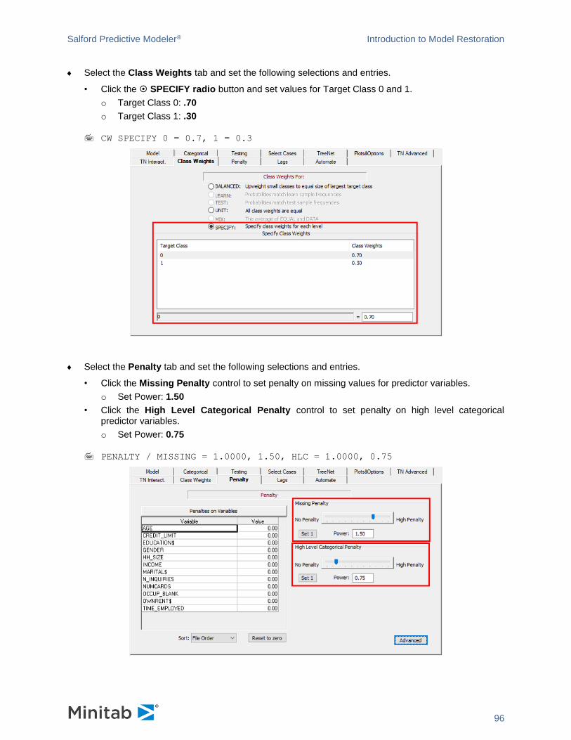
Salford Predictive Modeler® Introduction to Model Restoration
96
Select the Class Weights tab and set the following selections and entries.
• Click the SPECIFY radio button and set values for Target Class 0 and 1.
o Target Class 0: .70
o Target Class 1: .30
CW SPECIFY 0 = 0.7, 1 = 0.3
Select the Penalty tab and set the following selections and entries.
• Click the Missing Penalty control to set penalty on missing values for predictor variables.
o Set Power: 1.50
• Click the High Level Categorical Penalty control to set penalty on high level categorical predictor variables.
o Set Power: 0.75
PENALTY / MISSING = 1.0000, 1.50, HLC = 1.0000, 0.75

Salford Predictive Modeler® Introduction to Model Restoration
97
Saving the Grove File
Now that we have completed the model setup by defining of our model parameters, options, settings and
values, we need to ensure we save our work prior to, or after, launching and running the model.
Before we walk through saving the grove we need to define what the grove file is.
What is a grove file?
The grove file (.GRV) is a proprietary binary file (universal container) used by the SPM engine to store
any kind of modeling results. It includes complete information about the model-building process, including
the model itself. For example, the TreeNet® modeling engine will generate a series of trees, performance
statistics, dependency plots, interaction reports and other pieces of information. All these details will be
saved into the grove file.
The grove can be used to score new data and to produce descriptive information about the scoring
process (performance stats, prediction success table, etc.). The grove can also be used to translate the
model into one of the supported languages.
SPM can display the modeling results saved to a grove just like it does for a model you build in the
current session. In fact, if one does not specify a grove file, a temporary file will be created.
Depending on workflow, one could specify a named grove file for the analysis using the [Save Grove…]
button in the model results window.
The grove file will be created on your hard drive only after the process is completely finished. You won’t be able to create more plots using interactive GUI controls after you save the model.
✓ Specifying Grove file name in advance makes sense for analyses that take a long time to run.
✓ You can also save the grove file from the results window (see below) after the run is finished.
GROVE <file>
Grove contains “engine state”
The grove file (.GRV) now contains the “engine state”. The engine state allows SPM to collect all user
settings into a session object which is now saved as part of the grove structure. This allows the grove to
be saved and later recalled in a new session at any point in time. Upon saving and recalling of the
session, the principal goal is to be able to capture and save a comprehensive set of user parameters and
settings at any moment in time during a model building session. This is the "state of the engine", or
“engine state”. It represents the history of a session leading up to any given point in time, complete with
hundreds of user options.
Another way to think about it is that at any given point in time during a modeling session, the user might
launch a modeling session via an action command, or via a GUI control. It is at that moment that the user
has both a history (of actions during the session) and a state. The history constitutes all the actions the
user has taken during the session, while the state represents the settings of all SPM control parameters
at a given point in time.
When any GUI action or command is given which starts a process, the user can elect to preserve the
state of the session by saving the grove (.GRV).
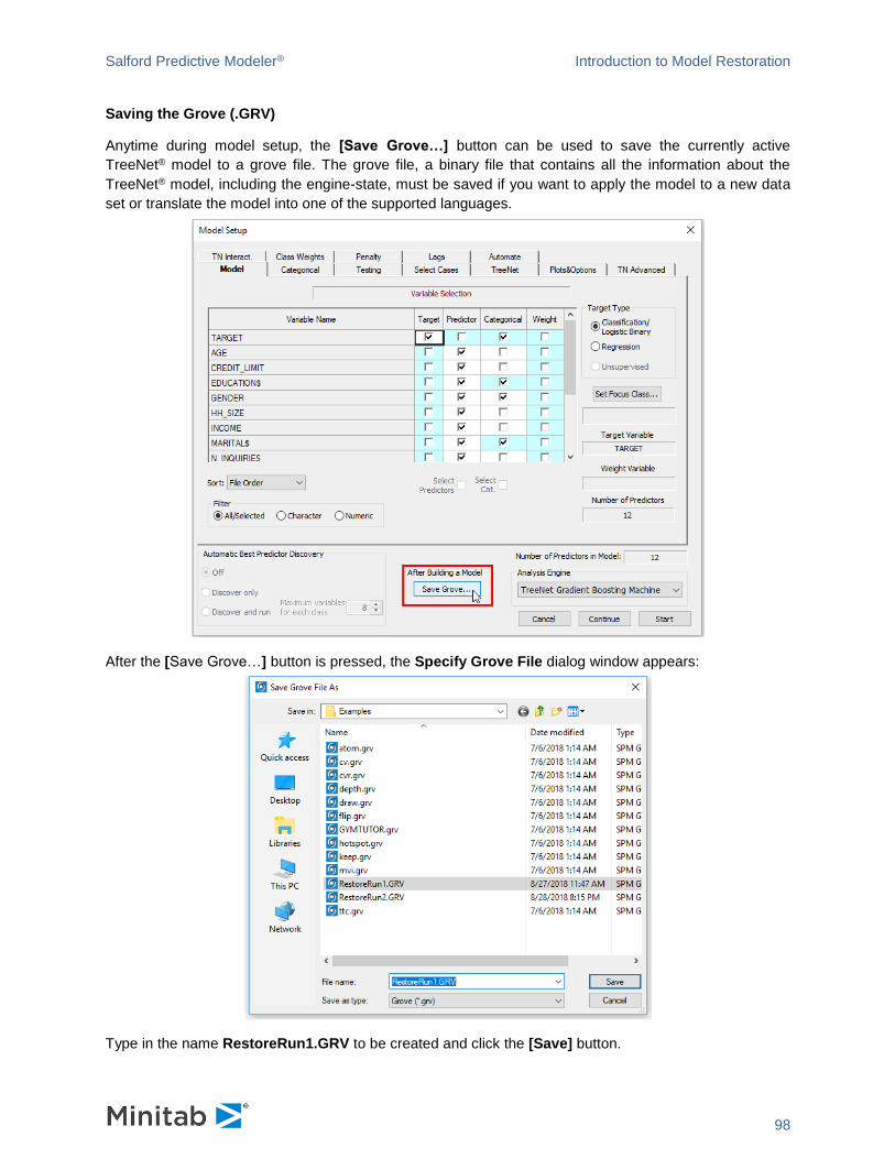
Salford Predictive Modeler® Introduction to Model Restoration
98
Saving the Grove (.GRV)
Anytime during model setup, the [Save Grove…] button can be used to save the currently active
TreeNet® model to a grove file. The grove file, a binary file that contains all the information about the
TreeNet® model, including the engine-state, must be saved if you want to apply the model to a new data
set or translate the model into one of the supported languages.
After the [Save Grove…] button is pressed, the Specify Grove File dialog window appears:
Type in the name RestoreRun1.GRV to be created and click the [Save] button.
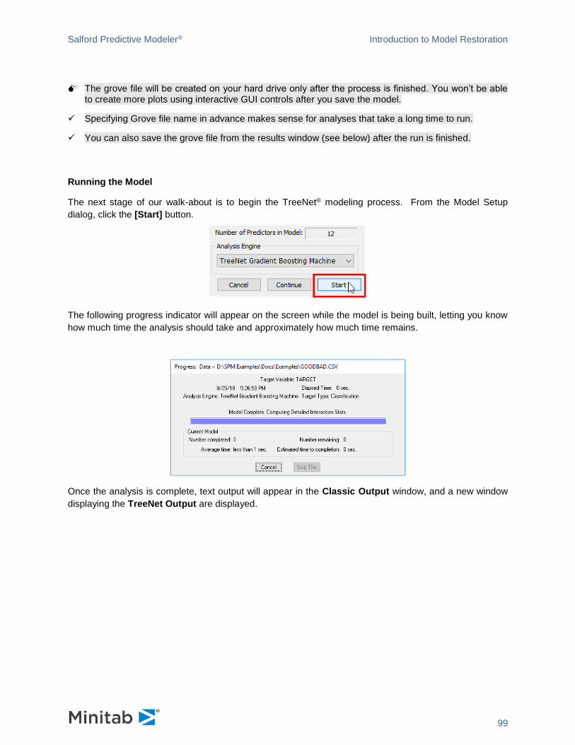
Salford Predictive Modeler® Introduction to Model Restoration
99
The grove file will be created on your hard drive only after the process is finished. You won’t be able to create more plots using interactive GUI controls after you save the model.
✓ Specifying Grove file name in advance makes sense for analyses that take a long time to run.
✓ You can also save the grove file from the results window (see below) after the run is finished.
Running the Model
The next stage of our walk-about is to begin the TreeNet® modeling process. From the Model Setup
dialog, click the [Start] button.
The following progress indicator will appear on the screen while the model is being built, letting you know
how much time the analysis should take and approximately how much time remains.
Once the analysis is complete, text output will appear in the Classic Output window, and a new window
displaying the TreeNet Output are displayed.
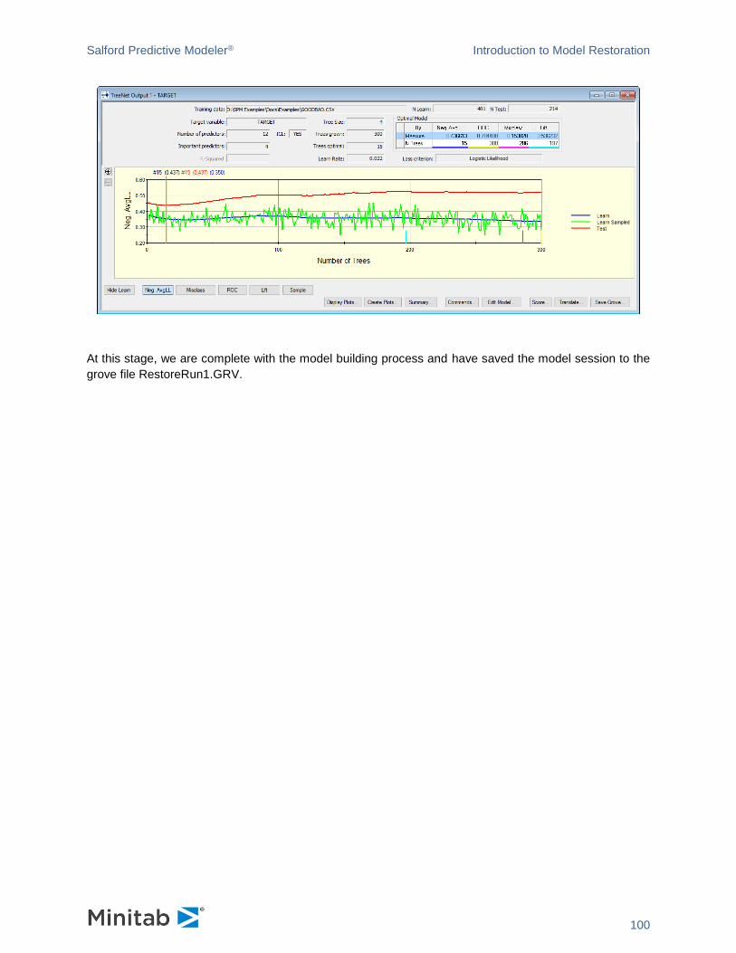
Salford Predictive Modeler® Introduction to Model Restoration
100
At this stage, we are complete with the model building process and have saved the model session to the
grove file RestoreRun1.GRV.
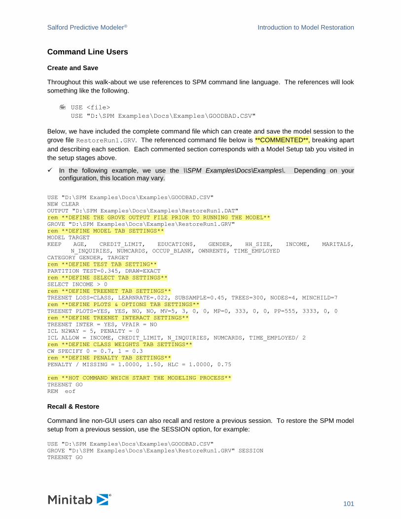
Salford Predictive Modeler® Introduction to Model Restoration
101
Command Line Users
Create and Save
Throughout this walk-about we use references to SPM command line language. The references will look
something like the following.
USE <file>
USE "D:\SPM Examples\Docs\Examples\GOODBAD.CSV"
Below, we have included the complete command file which can create and save the model session to the
grove file RestoreRun1.GRV. The referenced command file below is **COMMENTED**, breaking apart
and describing each section. Each commented section corresponds with a Model Setup tab you visited in
the setup stages above.
✓ In the following example, we use the \\SPM Examples\Docs\Examples\. Depending on your configuration, this location may vary.
USE "D:\SPM Examples\Docs\Examples\GOODBAD.CSV"
NEW CLEAR
OUTPUT "D:\SPM Examples\Docs\Examples\RestoreRun1.DAT"
rem **DEFINE THE GROVE OUTPUT FILE PRIOR TO RUNNING THE MODEL**
GROVE "D:\SPM Examples\Docs\Examples\RestoreRun1.GRV"
rem **DEFINE MODEL TAB SETTINGS**
MODEL TARGET
KEEP AGE, CREDIT_LIMIT, EDUCATION$, GENDER, HH_SIZE, INCOME, MARITAL$,
N_INQUIRIES, NUMCARDS, OCCUP_BLANK, OWNRENT$, TIME_EMPLOYED
CATEGORY GENDER, TARGET
rem **DEFINE TEST TAB SETTING**
PARTITION TEST=0.345, DRAW=EXACT
rem **DEFINE SELECT TAB SETTINGS**
SELECT INCOME > 0
rem **DEFINE TREENET TAB SETTINGS**
TREENET LOSS=CLASS, LEARNRATE=.022, SUBSAMPLE=0.45, TREES=300, NODES=4, MINCHILD=7
rem **DEFINE PLOTS & OPTIONS TAB SETTINGS**
TREENET PLOTS=YES, YES, NO, NO, MV=5, 3, 0, 0, MP=0, 333, 0, 0, PP=555, 3333, 0, 0
rem **DEFINE TREENET INTERACT SETTINGS**
TREENET INTER = YES, VPAIR = NO
ICL N2WAY = 5, PENALTY = 0
ICL ALLOW = INCOME, CREDIT_LIMIT, N_INQUIRIES, NUMCARDS, TIME_EMPLOYED/ 2
rem **DEFINE CLASS WEIGHTS TAB SETTINGS**
CW SPECIFY 0 = 0.7, 1 = 0.3
rem **DEFINE PENALTY TAB SETTINGS**
PENALTY / MISSING = 1.0000, 1.50, HLC = 1.0000, 0.75
rem **HOT COMMAND WHICH START THE MODELING PROCESS**
TREENET GO
REM eof
Recall & Restore
Command line non-GUI users can also recall and restore a previous session. To restore the SPM model
setup from a previous session, use the SESSION option, for example:
USE "D:\SPM Examples\Docs\Examples\GOODBAD.CSV"
GROVE "D:\SPM Examples\Docs\Examples\RestoreRun1.GRV" SESSION
TREENET GO

Salford Predictive Modeler® Introduction to Model Restoration
102
Session Recall & Restore
The next stage of this walk-about is to revisit the grove file we created in the previous stage and open it
within the SPM user interface allowing you to recall and restore the previous TreeNet® model that we
patiently set up.
Requirements and Approaches
There are several requirements you should understand about the model restoration process.
• Groves must be created and saved in SPM v8.3.
o While earlier versions of groves can still be used for model viewing, scoring, and translation, the restore and recall functionality is not supported for grove files created with earlier versions of SPM.
• Input Data File
o File names: There are no additional requirements other than the standard SPM input data file requirements. By default, the process will first look for the original filenames and directory path used to create the model.
• Variable names
o Original variables: Every variable that was used to build the model when the session state was created must be present in the input data used during the recall and restore process. If any of the variables expected is not available, the process will stop with variable mismatch.
o Variable ordering: The recall and restore process is agnostic to the order in which variables are arranged within the input data file.
o Different variable count: There are no issues with additional variables appearing within the input data file if the original modeling variables are present.
Paths to Successful Recall/Restore
There are several paths one could choose to recall and restore the session state. All of them have to do
with three main questions we can ask sequentially to determine the next step following the opening of a
grove (.GRV) file. They are as follows. After opening a grove and selecting the option:
Q1.) Does the user want to restore engine session (YES/NO)?
a. If YES, then ask Q2.
b. If NO, stop and open standard results window.
Q2.) Is there a data file open (YES/NO)?
a. If YES, then ask Q3.
b. If NO, pause and display the Open Data File window identifying the original filename to
locate. This pause allows the user to locate and open a data file selected for
recalling/restoring the session state.
Q3.) Do all the variables needed by the session being recalled appear in the selected data file
(YES/NO)?
a. If YES, stop and return users to model setup dialog with restored session state available.
b. If NO, stop and open standard results window.
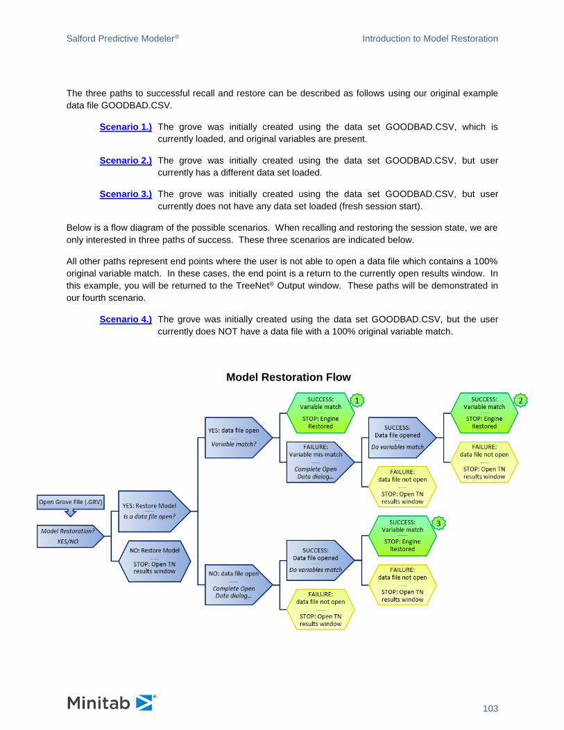
Salford Predictive Modeler® Introduction to Model Restoration
103
The three paths to successful recall and restore can be described as follows using our original example
data file GOODBAD.CSV.
Scenario 1.) The grove was initially created using the data set GOODBAD.CSV, which is
currently loaded, and original variables are present.
Scenario 2.) The grove was initially created using the data set GOODBAD.CSV, but user
currently has a different data set loaded.
Scenario 3.) The grove was initially created using the data set GOODBAD.CSV, but user
currently does not have any data set loaded (fresh session start).
Below is a flow diagram of the possible scenarios. When recalling and restoring the session state, we are
only interested in three paths of success. These three scenarios are indicated below.
All other paths represent end points where the user is not able to open a data file which contains a 100%
original variable match. In these cases, the end point is a return to the currently open results window. In
this example, you will be returned to the TreeNet® Output window. These paths will be demonstrated in
our fourth scenario.
Scenario 4.) The grove was initially created using the data set GOODBAD.CSV, but the user
currently does NOT have a data file with a 100% original variable match.
Model Restoration Flow
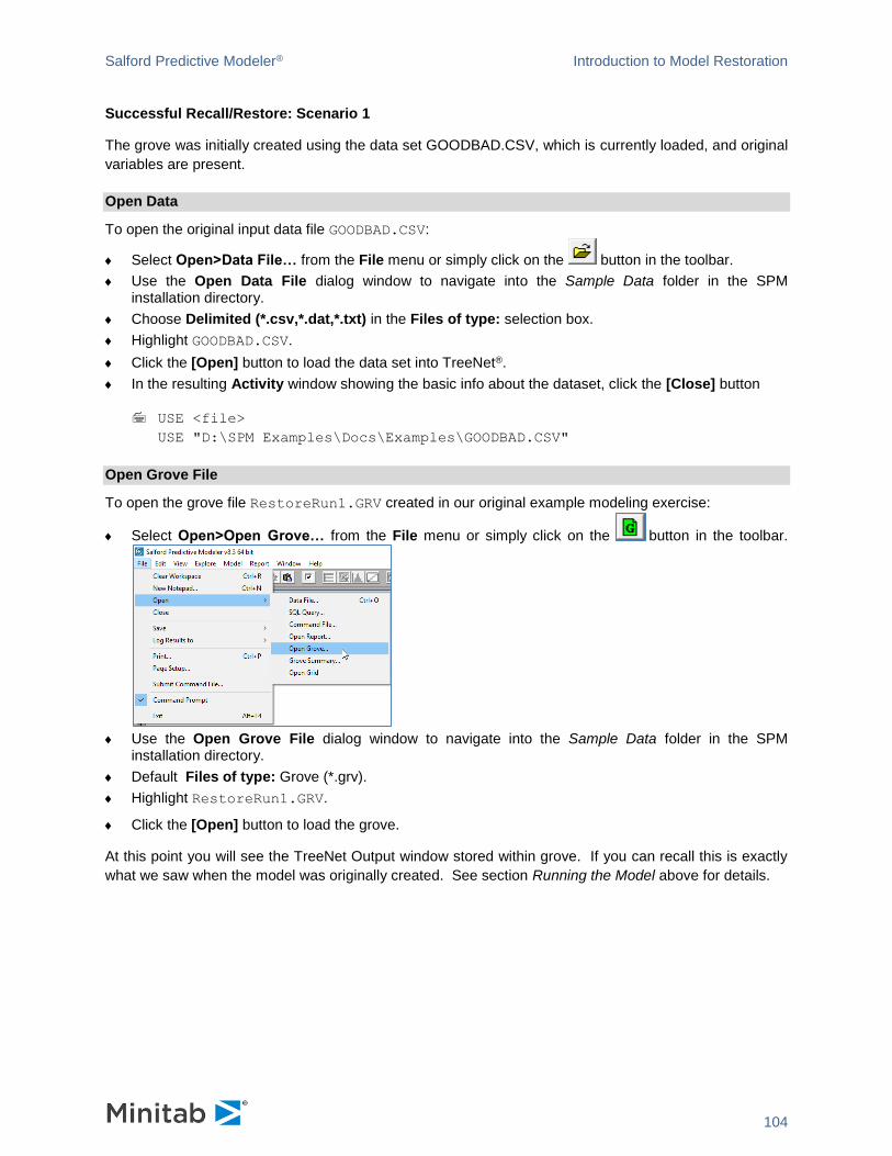
Salford Predictive Modeler® Introduction to Model Restoration
104
Successful Recall/Restore: Scenario 1
The grove was initially created using the data set GOODBAD.CSV, which is currently loaded, and original
variables are present.
Open Data
To open the original input data file GOODBAD.CSV:
Select Open>Data File… from the File menu or simply click on the button in the toolbar.
Use the Open Data File dialog window to navigate into the Sample Data folder in the SPM installation directory.
Choose Delimited (*.csv,*.dat,*.txt) in the Files of type: selection box.
Highlight GOODBAD.CSV.
Click the [Open] button to load the data set into TreeNet®.
In the resulting Activity window showing the basic info about the dataset, click the [Close] button
USE <file>
USE "D:\SPM Examples\Docs\Examples\GOODBAD.CSV"
Open Grove File
To open the grove file RestoreRun1.GRV created in our original example modeling exercise:
Select Open>Open Grove… from the File menu or simply click on the button in the toolbar.
Use the Open Grove File dialog window to navigate into the Sample Data folder in the SPM installation directory.
Default Files of type: Grove (*.grv).
Highlight RestoreRun1.GRV.
Click the [Open] button to load the grove.
At this point you will see the TreeNet Output window stored within grove. If you can recall this is exactly
what we saw when the model was originally created. See section Running the Model above for details.
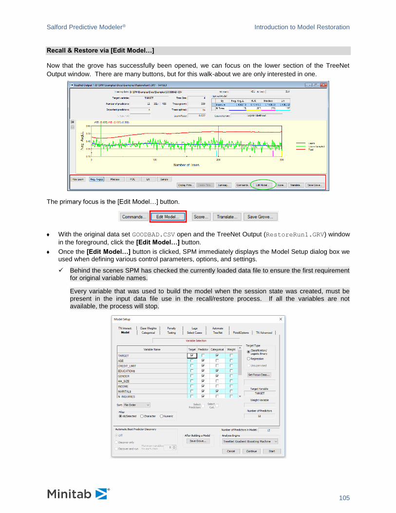
Salford Predictive Modeler® Introduction to Model Restoration
105
Recall & Restore via [Edit Model…]
Now that the grove has successfully been opened, we can focus on the lower section of the TreeNet
Output window. There are many buttons, but for this walk-about we are only interested in one.
The primary focus is the [Edit Model…] button.
With the original data set GOODBAD.CSV open and the TreeNet Output (RestoreRun1.GRV) window
in the foreground, click the [Edit Model…] button.
Once the [Edit Model…] button is clicked, SPM immediately displays the Model Setup dialog box we used when defining various control parameters, options, and settings.
✓ Behind the scenes SPM has checked the currently loaded data file to ensure the first requirement for original variable names.
Every variable that was used to build the model when the session state was created, must be present in the input data file use in the recall/restore process. If all the variables are not available, the process will stop.
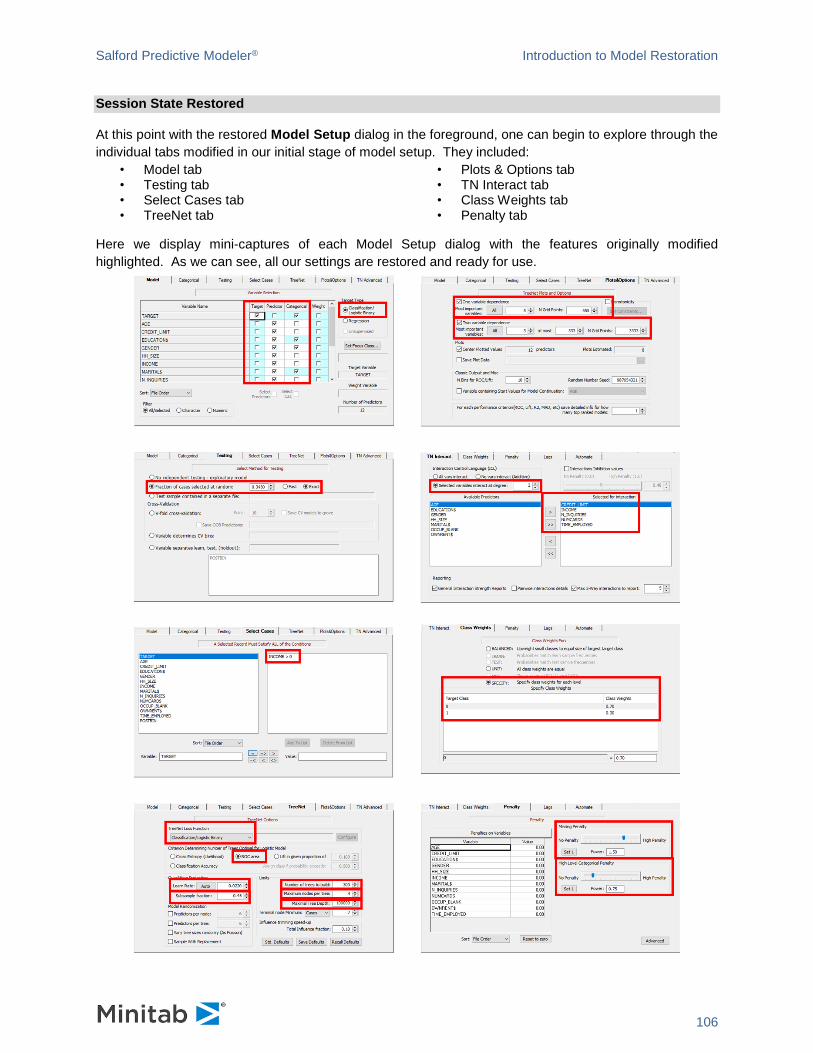
Salford Predictive Modeler® Introduction to Model Restoration
106
Session State Restored
At this point with the restored Model Setup dialog in the foreground, one can begin to explore through the
individual tabs modified in our initial stage of model setup. They included:
• Model tab • Testing tab • Select Cases tab • TreeNet tab
• Plots & Options tab • TN Interact tab • Class Weights tab • Penalty tab
Here we display mini-captures of each Model Setup dialog with the features originally modified
highlighted. As we can see, all our settings are restored and ready for use.

Salford Predictive Modeler® Introduction to Model Restoration
107
Next Steps
With the model session restored, you are now able to:
Recreate your model. As an exercise, at this point we can replicate our original model by clicking the [Start] button.
Quickly modify the various control parameters, options, and settings of the model.
Scenario 1: Conclusion and Summary
Opened original data file GOODBAD.CSV.
Opened original model session stored in RestoreRun1.GRV.
Restored model session by clicking the [Edit Model…] button.
Began working with successfully restored model session.
This concludes the Scenario 1 walk-about. Please see other Successful Recall/Restore: Scenario # for
further examples.

Salford Predictive Modeler® Introduction to Model Restoration
108
Successful Recall/Restore: Scenario 2
The grove was initially created using the data set GOODBAD.CSV, but user currently has a new and
different data set loaded which contains variable mis-matches.
Open Data
For this scenario, we are using a different data file rather than the original GOODBAD.CSV. This
example will start with the data file GYMTUTOR.CSV. This is just another data file which can be
found the Sample Data folder. We are using GYMTUTOR.CSV because this scenario demonstrates
what occurs when the user attempts to recall/restore a session when the original model variables are not present in active data file.
Select Open>Data File… from the File menu or simply click on the button in the toolbar.
Use the Open Data File dialog window to navigate into the Sample Data folder in the SPM installation directory.
Choose Delimited (*.csv,*.dat,*.txt) in the Files of type: selection box.
Highlight GYMTUTOR.CSV.
Click the [Open] button to load the data set into TreeNet®.
In the resulting Activity window showing the basic info about the dataset, click the [Close] button
USE <file>
USE "D:\SPM Examples\Docs\Examples\GYMTUTOR.CSV"
Open Grove File
To open the grove file RestoreRun1.GRV created in our original example modeling exercise:
Select Open>Open Grove… from the File menu or simply click on the button in the toolbar. See “Successful Recall/Restore: Scenario 1” for more details.
Use the Open Grove File dialog window to navigate into the Sample Data folder in the SPM installation directory.
Default Files of type: Grove (*.grv).
Highlight RestoreRun1.GRV.
Click the [Open] button to load the grove.
At this point you will see the TreeNet® Output window stored within grove. If you can recall this is exactly
what we saw when the model was originally created. See section Running the Model above for details.
Recall & Restore via [Edit Model…]
Now that the grove has successfully been open, we can focus on the lower section of the TreeNet Output
window. There are many buttons, but for this walk-about we are only interested in one. The primary
focus is the [Edit Model…] button.
With the original data set GOODBAD.CSV open and the TreeNet Output (RestoreRun1.GRV) window
in the foreground, click the [Edit Model…] button.
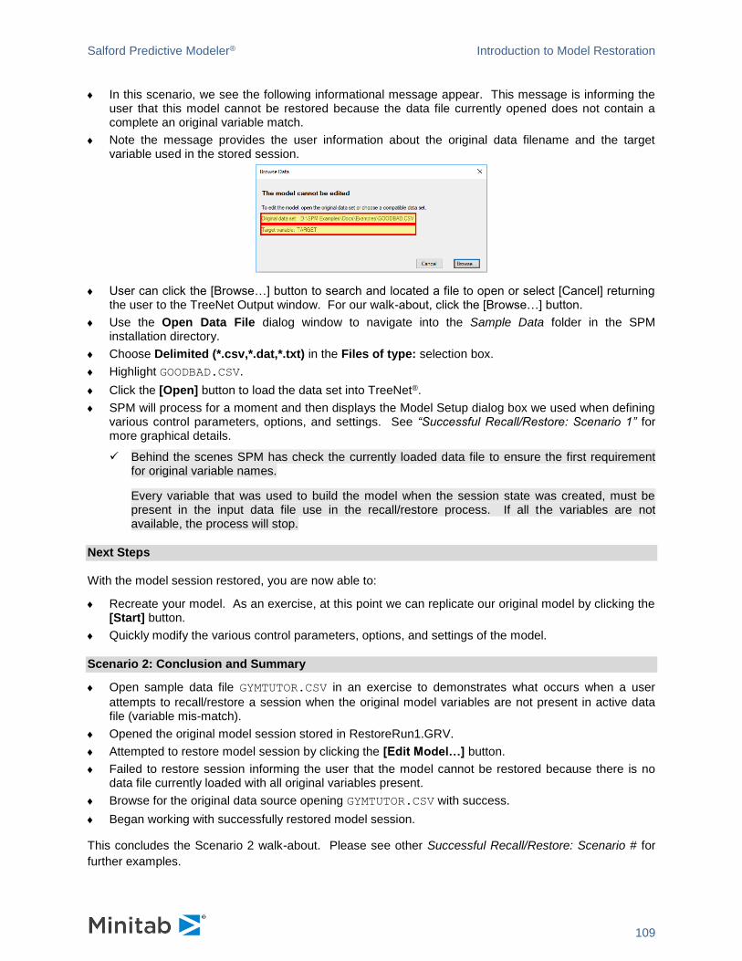
Salford Predictive Modeler® Introduction to Model Restoration
109
In this scenario, we see the following informational message appear. This message is informing the user that this model cannot be restored because the data file currently opened does not contain a complete an original variable match.
Note the message provides the user information about the original data filename and the target variable used in the stored session.
User can click the [Browse…] button to search and located a file to open or select [Cancel] returning the user to the TreeNet Output window. For our walk-about, click the [Browse…] button.
Use the Open Data File dialog window to navigate into the Sample Data folder in the SPM installation directory.
Choose Delimited (*.csv,*.dat,*.txt) in the Files of type: selection box.
Highlight GOODBAD.CSV.
Click the [Open] button to load the data set into TreeNet®.
SPM will process for a moment and then displays the Model Setup dialog box we used when defining various control parameters, options, and settings. See “Successful Recall/Restore: Scenario 1” for more graphical details.
✓ Behind the scenes SPM has check the currently loaded data file to ensure the first requirement for original variable names.
Every variable that was used to build the model when the session state was created, must be present in the input data file use in the recall/restore process. If all the variables are not available, the process will stop.
Next Steps
With the model session restored, you are now able to:
Recreate your model. As an exercise, at this point we can replicate our original model by clicking the [Start] button.
Quickly modify the various control parameters, options, and settings of the model.
Scenario 2: Conclusion and Summary
Open sample data file GYMTUTOR.CSV in an exercise to demonstrates what occurs when a user
attempts to recall/restore a session when the original model variables are not present in active data file (variable mis-match).
Opened the original model session stored in RestoreRun1.GRV.
Attempted to restore model session by clicking the [Edit Model…] button.
Failed to restore session informing the user that the model cannot be restored because there is no data file currently loaded with all original variables present.
Browse for the original data source opening GYMTUTOR.CSV with success.
Began working with successfully restored model session.
This concludes the Scenario 2 walk-about. Please see other Successful Recall/Restore: Scenario # for
further examples.
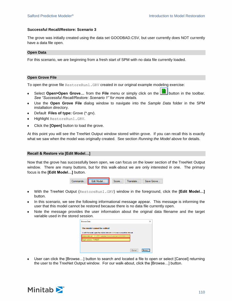
Salford Predictive Modeler® Introduction to Model Restoration
110
Successful Recall/Restore: Scenario 3
The grove was initially created using the data set GOODBAD.CSV, but user currently does NOT currently
have a data file open.
Open Data
For this scenario, we are beginning from a fresh start of SPM with no data file currently loaded.
Open Grove File
To open the grove file RestoreRun1.GRV created in our original example modeling exercise:
Select Open>Open Grove… from the File menu or simply click on the button in the toolbar. See “Successful Recall/Restore: Scenario 1” for more details.
Use the Open Grove File dialog window to navigate into the Sample Data folder in the SPM installation directory.
Default Files of type: Grove (*.grv).
Highlight RestoreRun1.GRV.
Click the [Open] button to load the grove.
At this point you will see the TreeNet Output window stored within grove. If you can recall this is exactly
what we saw when the model was originally created. See section Running the Model above for details.
Recall & Restore via [Edit Model…]
Now that the grove has successfully been open, we can focus on the lower section of the TreeNet Output
window. There are many buttons, but for this walk-about we are only interested in one. The primary
focus is the [Edit Model…] button.
With the TreeNet Output (RestoreRun1.GRV) window in the foreground, click the [Edit Model…]
button.
In this scenario, we see the following informational message appear. This message is informing the user that this model cannot be restored because there is no data file currently open.
Note the message provides the user information about the original data filename and the target variable used in the stored session.
User can click the [Browse…] button to search and located a file to open or select [Cancel] returning the user to the TreeNet Output window. For our walk-about, click the [Browse…] button.

Salford Predictive Modeler® Introduction to Model Restoration
111
Use the Open Data File dialog window to navigate into the Sample Data folder in the SPM installation directory.
Choose Delimited (*.csv,*.dat,*.txt) in the Files of type: selection box.
Highlight GOODBADmorevariables.csv.
Click the [Open] button to load the data set into TreeNet®.
✓ NOTE: We are using a different data file GOODBADmorevariables.csv. It is a version of the
original data file with ten additional variables added (x1-x10). This addition to the scenario demonstrates that SPM does not care if additional variables are part of the data file if the first requirement is passed.
SPM will process for a moment and then displays the Model Setup dialog box we used when defining various control parameters, options, and settings. See “Successful Recall/Restore: Scenario 1” for more graphical details.
✓ Behind the scenes SPM has check the currently loaded data file to ensure the first requirement for original variable names.
Every variable that was used to build the model when the session state was created, must be present in the input data file use in the recall/restore process. If all the variables are not available, the process will stop.
Next Steps
With the model session restored, you are now able to:
Recreate your model. As an exercise, at this point we can replicate our original model by clicking the [Start] button.
Use the restored session as the starting point of additional modeling sessions.
Quickly modify the various control parameters, options, and settings of the model.
Continue to work with RestoreRun1.GRV in other tasks like scoring new data or translating the model into one of the supported languages later.
Scenario 3: Conclusion and Summary
From a fresh SPM start with no data file loaded, opened the original model session stored in RestoreRun1.GRV.
Attempted to restore model session by clicking the [Edit Model…] button.
Failed to restore session informing the user that the model cannot be restored because there is no data file currently open.
Browse for the original data source opening GYMTUTOR.CSV with success.
Began working with successfully restored model session.
This concludes the Scenario 3 walk-about. Please see other Successful Recall/Restore: Scenario # for
further examples.
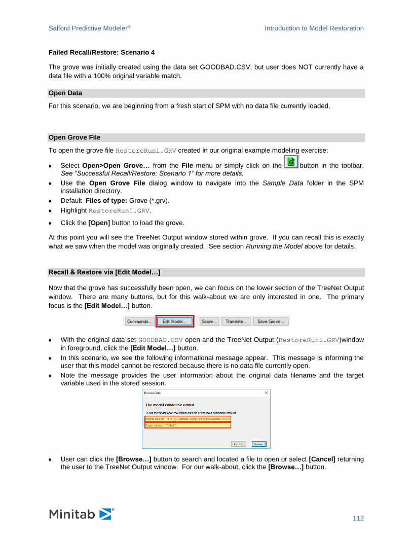
Salford Predictive Modeler® Introduction to Model Restoration
112
Failed Recall/Restore: Scenario 4
The grove was initially created using the data set GOODBAD.CSV, but user does NOT currently have a
data file with a 100% original variable match.
Open Data
For this scenario, we are beginning from a fresh start of SPM with no data file currently loaded.
Open Grove File
To open the grove file RestoreRun1.GRV created in our original example modeling exercise:
Select Open>Open Grove… from the File menu or simply click on the button in the toolbar. See “Successful Recall/Restore: Scenario 1” for more details.
Use the Open Grove File dialog window to navigate into the Sample Data folder in the SPM installation directory.
Default Files of type: Grove (*.grv).
Highlight RestoreRun1.GRV.
Click the [Open] button to load the grove.
At this point you will see the TreeNet Output window stored within grove. If you can recall this is exactly
what we saw when the model was originally created. See section Running the Model above for details.
Recall & Restore via [Edit Model…]
Now that the grove has successfully been open, we can focus on the lower section of the TreeNet Output
window. There are many buttons, but for this walk-about we are only interested in one. The primary
focus is the [Edit Model…] button.
With the original data set GOODBAD.CSV open and the TreeNet Output (RestoreRun1.GRV)window
in foreground, click the [Edit Model…] button.
In this scenario, we see the following informational message appear. This message is informing the user that this model cannot be restored because there is no data file currently open.
Note the message provides the user information about the original data filename and the target variable used in the stored session.
User can click the [Browse…] button to search and located a file to open or select [Cancel] returning the user to the TreeNet Output window. For our walk-about, click the [Browse…] button.
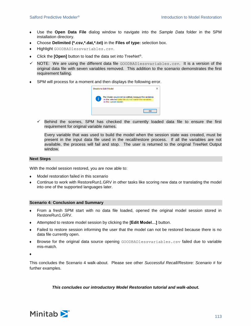
Salford Predictive Modeler® Introduction to Model Restoration
113
Use the Open Data File dialog window to navigate into the Sample Data folder in the SPM installation directory.
Choose Delimited (*.csv,*.dat,*.txt) in the Files of type: selection box.
Highlight GOODBADlessvariables.csv.
Click the [Open] button to load the data set into TreeNet®.
✓ NOTE: We are using the different data file GOODBADlessvariables.csv. It is a version of the
original data file with seven variables removed. This addition to the scenario demonstrates the first requirement failing.
SPM will process for a moment and then displays the following error.
✓ Behind the scenes, SPM has checked the currently loaded data file to ensure the first requirement for original variable names.
Every variable that was used to build the model when the session state was created, must be present in the input data file used in the recall/restore process. If all the variables are not available, the process will fail and stop. The user is returned to the original TreeNet Output window.
Next Steps
With the model session restored, you are now able to:
Model restoration failed in this scenario
Continue to work with RestoreRun1.GRV in other tasks like scoring new data or translating the model into one of the supported languages later.
Scenario 4: Conclusion and Summary
From a fresh SPM start with no data file loaded, opened the original model session stored in RestoreRun1.GRV.
Attempted to restore model session by clicking the [Edit Model…] button.
Failed to restore session informing the user that the model can not be restored because there is no data file currently open.
Browse for the original data source opening GOODBADlessvariables.csv failed due to variable
mis-match.
This concludes the Scenario 4 walk-about. Please see other Successful Recall/Restore: Scenario # for
further examples.
This concludes our introductory Model Restoration tutorial and walk-about.

Salford Predictive Modeler® Introduction to Model Restoration
114
UNIX/Console Usage Notes
The nature of UNIX-like operating environments affects the operation of the SPM in non-trivial ways. This
section discusses the operation of the SPM in the UNIX operating environment and the operation of
console (non-GUI) SPM in general. Both GUI and console SPM are offered for Windows; only the console
is offered for UNIX or Linux.
Case Sensitivity
The SPM command interpreter is case-insensitive; in fact, commands are generally converted internally
to upper-case letters. The only exception to this rule is that the text placed between quotation marks is
not converted, remaining in its original case. UNIX file systems, on the other hand, are case-sensitive,
meaning that upper and lower case letters are treated as completely different characters. Thus, one could
not refer to a file named “this.csv” as “THIS.CSV,” or vice-versa.
It is therefore important to remember that unquoted filenames are assumed to be upper case; lower and
mixed case names must be quoted.
Use Caution When Transferring PC Files
It is always important to use binary mode when copying non-text files from a DOS/Windows environment
to a UNIX environment (or vice-versa). Failure to do so will cause the files to be corrupted.
Supporting Database Conversion Libraries
On selected platforms, the SPM will use the Stat/Transfer database engine to read and write any file
format supported by Stat/Transfer.
The SPM executable can function without Stat/Transfer interface. Proper installation for supported platform installs Stat/Transfer modules too and makes them discoverable by SPM.
To access data through the Stat/Transfer interface, one simply uses the USE, SAVE, or PROPORTION
FILE commands; the file name must be quoted.
To disable the Stat/Transfer interface, one can use the command "LOPTIONS STATTRAN=NO"; likewise, to re-enable the Stat/Transfer interface, one uses the command "LOPTIONS STATTRAN=YES".
If data translation engine is disabled, the only supported file format is plain-text CSV.
✓ Since v6, SPM includes native support for text datasets, which are, for many users, the most flexible and natural formats in which to maintain data. A single delimiter is used throughout the dataset. It is usually a comma, but semicolon, space, and tab are also supported as delimiters.
The FPATH Command
The FPATH command can be used to specify locations for different types of input and output files. For
example, the following command will cause SPM to read and write files in the directory “Salford,” under
your home directory by default (on UNIX-like systems):
FPATH “~Salford”
Thereafter, if one gives an input/output command such as USE, OUTPUT, or SAVE, SPM will look in
~/Salford unless the filename is quoted or the FPATH command is canceled by giving an FPATH
command without arguments.
Salford Predictive Modeler® Introduction to Model Restoration
115
One can also specify different default directories for different sorts of files. To specify a default directory
for input datasets, use:
FPATH <pathname> /use
To specify a default directory for output datasets, use:
FPATH <pathname> /save
For command files, use:
FPATH <pathname> /submit
For text output files, use:
FPATH <pathname> /output
FPATH without arguments restores the default, which is to use the current working directory. FPATH with
an option but no pathname restores the default for the specified file type.
Built-in Help
HELP [<command>]
Console SPM has its own built-in help system, which can be accessed by opening the SPM in interactive
mode and typing "HELP" at the prompt. To read the entry for a particular command, type “HELP” followed
by the name of the command.
Workspace Allocation
Console SPM can allocate arbitrary amounts of memory. The default workspace size is 25 MB, but this
can be altered with either the SALFORD_M environment variable, or the -m command line flag. We
suggest that SALFORD_M be set in the system-wide startup files (/etc/profile and /etc/csh.login on most
UNIX-like systems), as appropriate for the hardware.
Limit on Number of Variables
By default, the SPM will read datasets with up to 32,768 variables. This number can be increased with the
-v command line flag.
Modes of Operation
Console SPM can be invoked interactively by launching it at the command prompt without arguments.
You will get a series of startup messages looking something like this:
This launch supports up to 32768 variables.
This launch supports unlimited data.
Salford Predictive Modeler(R) software suite version 8.3.0.001
CART(R) ProEx, TreeNet(R) ProEX, MARS(R) ProEX, RandomForests(R) ProEX,
GPS/Generalized Lasso(TM) ProEX, RuleLearner(R), ISLE, Logit ProEX,
REGRESS ProEX
Copyright, 1991-2018, Salford Systems, San Diego, California, USA
Salford Predictive Modeler® Introduction to Model Restoration
116
SPM Salford Predictive Modeler(R) software suite includes selected
versions of the following:
CART(R) (c)1984-2018 California Statistical Software, Inc.
TreeNet(R) (c)2001-2018 Salford Systems
MARS(R) (c)1991-2018 Jeril, Inc.
RandomForests(R) (c)2002-2018 Leo Breiman, Adele Cutler and Salford Systems
PRIM(TM) (c)1997-2018 Jeril, Inc.
GeneralizedPathSeeker(TM) (c)2009-2018 Jeril, Inc.
PathSeeker(TM) (c)2004-2018 Jeril, Inc.
RuleLearner(R) (c)2012-2018 Salford Systems
ISLE (c)2012-2018 Salford Systems
2SLS (c)1988-2018 Salford Systems
SPM uses zlib software from www.zlib.net
SPM uses LZ compression.
The license supports unlimited learn sample data.
You can then enter commands and receive responses. Your session ends when you enter the QUIT
command.
Since the SPM in interactive mode will accept commands through standard input and send responses
through standard output, it is sometimes convenient to invoke it in the following way from a script or batch
file. For example, the commands below read the SPM commands from a set of command files and write
results to output.dat.
$ cat runit1.cmd runit2.cmd runit3.cmd|SPM >output.dat
Generally, the more convenient way to run console SPM is in batch mode, which can be invoked by
specifying a command file as an argument. For example, let’s execute runit1.cmd in batch mode.
$ SPM runit1.cmd
When operating in batch mode, the SPM does not send any output to your screen, other than startup and
error messages, unless ECHO ON is in effect, or the -e command line flag has been specified. It is
therefore a good idea to specify an output file with the OUTPUT command inside your command file.
Otherwise you may never see Classic Output results at all. The SPM will terminate either when it has
encountered a QUIT command, or there are no more commands to be executed.
Startup File
When console SPM is started in interactive mode, it looks for a file named SALFORD.CMD, first in your
current working directory and then in the directory pointed to by the SALFORD environment variable. If
the file is found, the SPM will execute its contents before displaying the command prompt. This allows
one to specify default settings for all Salford Systems applications. SALFORD.CMD is not automatically
executed in batch mode.
Command Line Startup Options
The SPM has a number of other command-line options. You can get the list of options by invoking the
SPM with the -h flag.
Salford Predictive Modeler® Introduction to Model Restoration
117
The command line syntax is:
SPM [options] [commandfile] [options]
Options are:
-e Echo results to console
-q Quiet, suppress all output including errors
-o<output_file> Direct text results to a file
-u<use_file> Attach to a dataset
-g<use_file> Identify a grove file
-w<Path> Identify Stat/Transfer dll path
-t<Path> Identify scratch file path
-s<MBytes> Data amount in MB, subject to license threshold
-m<MBytes> Model space in MB, subject to hardware limits
-l<optional_logfile> Error/warnings to text logfile
-mt<Nnumeric,Nchar> Lookup table capacities, 0 to grow without bound
-v<N> Specifies max N variables for the session
Examples: SPM -e model1.cmd
SPM \DataMining\Jobs-1\simulate.cmd -q
SPM job1.cmd -o\RESULTS\job1.txt -u\AnalysisData\sample1.sys
SPM -u\MyData\joint_data.xls[xls5]
SPM -s512 -m128
Environment variables can be used in lieu of command line switches: SALFORD_S in lieu of -s
SALFORD_M in lieu of -m
Examples: SPM -e model1.cmd
SPM /DataMining/Jobs-1/simulate.cmd -q
SPM job1.cmd -o/RESULTS/job1.txt -u/AnalysisData/sample1.sys
SPM -d/Progra~1/DBMSCopy7 -u/MyData/joint_data.xls[xls5]
SPM -s512 -p64 -m128
Environment variables can be used in lieu of command line switches:
SALFORD_S in lieu of -s
SALFORD_M in lieu of -m

Salford Predictive Modeler® Introduction to Model Restoration
118
An Overview of Model Summary Window
Model Summary window is a unified way to represent information about the model. It’s usually
accessible from model results windows (e.g. CART Navigator, TreeNet Output) via the [Summary]
button.
✓ After some analyses, this is the default Results window.
The information in Model Summary window is organized in tabs. This chapter describes general ones,
the tabs that are applicable to several or all of the Analysis Engines.
Summary tab
Summary tab is usually the first tab in a Model Summary window.
Model group to the left lists Target variable name and counts of Observation, Predictors, and categories
of the Target. For Regression models, the Target is continuous and the word “Regression” is used to
indicate that.
In some cases we show additional information like number of coefficients for linear models.
Model error measures grid shows performance statistics for each data sample in the model. Depending
on Target Type and other aspects of the model, appropriate performance measures are available. The
screenshot above shows the Summary for a CART® Regression model. Some of the regression
performance measures (MSE, MAD, R-Sq., etc.) are universally used for regression models. Relative
Error is specific to CART® models.
Dataset tab
Dataset tab represents information about the dataset used to build the model. It contains sizes of each
data sample, statistical information about the Target and number of records that may have been deleted
by one of the following reasons:
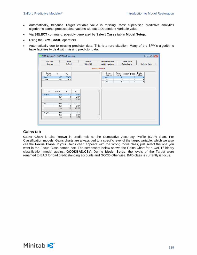
Salford Predictive Modeler® Introduction to Model Restoration
119
Automatically, because Target variable value is missing. Most supervised predictive analytics algorithms cannot process observations without a Dependent Variable value.
Via SELECT command, possibly generated by Select Cases tab in Model Setup.
Using the SPM BASIC operators.
Automatically due to missing predictor data. This is a rare situation. Many of the SPM’s algorithms have facilities to deal with missing predictor data.
Gains tab
Gains Chart is also known in credit risk as the Cumulative Accuracy Profile (CAP) chart. For Classification models, Gains charts are always tied to a specific level of the target variable, which we also call the Focus Class. If your Gains chart appears with the wrong focus class, just select the one you want in the Focus Class combo box. The screenshot below shows the Gains Chart for a CART® binary classification model against GOODBAD.CSV. During Model Setup, the levels of the Target were renamed to BAD for bad credit standing accounts and GOOD otherwise. BAD class is currently is focus.
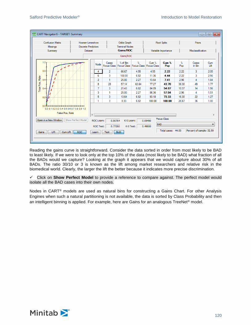
Salford Predictive Modeler® Introduction to Model Restoration
120
Reading the gains curve is straightforward. Consider the data sorted in order from most likely to be BAD to least likely. If we were to look only at the top 10% of the data (most likely to be BAD) what fraction of all the BADs would we capture? Looking at the graph it appears that we would capture about 30% of all BADs. The ratio 30/10 or 3 is known as the lift among market researchers and relative risk in the biomedical world. Clearly, the larger the lift the better because it indicates more precise discrimination.
✓ Click on Show Perfect Model to provide a reference to compare against. The perfect model would isolate all the BAD cases into their own nodes.
Nodes in CART® models are used as natural bins for constructing a Gains Chart. For other Analysis
Engines when such a natural partitioning is not available, the data is sorted by Class Probability and then
an intelligent binning is applied. For example, here are Gains for an analogous TreeNet® model.
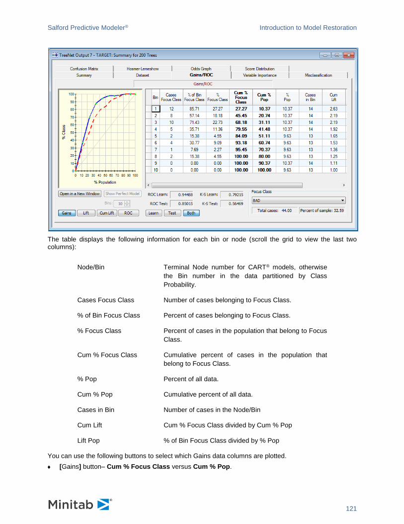
Salford Predictive Modeler® Introduction to Model Restoration
121
The table displays the following information for each bin or node (scroll the grid to view the last two columns):
Node/Bin Terminal Node number for CART® models, otherwise
the Bin number in the data partitioned by Class
Probability.
Cases Focus Class Number of cases belonging to Focus Class.
% of Bin Focus Class Percent of cases belonging to Focus Class.
% Focus Class Percent of cases in the population that belong to Focus
Class.
Cum % Focus Class Cumulative percent of cases in the population that
belong to Focus Class.
% Pop Percent of all data.
Cum % Pop Cumulative percent of all data.
Cases in Bin Number of cases in the Node/Bin
Cum Lift Cum % Focus Class divided by Cum % Pop
Lift Pop % of Bin Focus Class divided by % Pop
You can use the following buttons to select which Gains data columns are plotted.
[Gains] button– Cum % Focus Class versus Cum % Pop.
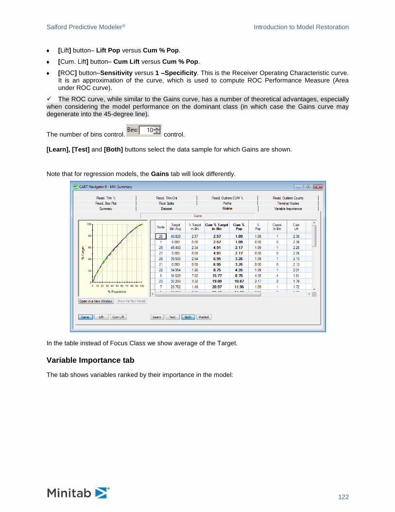
Salford Predictive Modeler® Introduction to Model Restoration
122
[Lift] button– Lift Pop versus Cum % Pop.
[Cum. Lift] button– Cum Lift versus Cum % Pop.
[ROC] button–Sensitivity versus 1 –Specificity. This is the Receiver Operating Characteristic curve. It is an approximation of the curve, which is used to compute ROC Performance Measure (Area under ROC curve).
✓ The ROC curve, while similar to the Gains curve, has a number of theoretical advantages, especially when considering the model performance on the dominant class (in which case the Gains curve may degenerate into the 45-degree line).
The number of bins control. control.
[Learn], [Test] and [Both] buttons select the data sample for which Gains are shown.
Note that for regression models, the Gains tab will look differently.
In the table instead of Focus Class we show average of the Target.
Variable Importance tab
The tab shows variables ranked by their importance in the model:

Salford Predictive Modeler® Introduction to Model Restoration
123
Each engine has a peculiar way to compute variable importance and might introduce specific features on
the tab. Please refer to the guide for a particular engine for more details. For example, here’s how
Variable Importance for a CART® model looks:
In any version of Variable Importance, you can highlight some variables in the grid and generate
commands to mark the selected variables as predictors using the [New Keep List] button. You can
request these commands to be applied at once via the [New Keep & Go] button. The [Select All] button
is a handy shortcut to select all the variables in the grid.
Relative importance checkbox toggles between raw and normalized scores.

Salford Predictive Modeler® Introduction to Model Restoration
124
Confusion Matrix tab
✓ This is a classification-only feature.
✓ This tab is called Prediction Success in previous versions of SPM.
The confusion matrix is a standard summary for classifiers of all kinds and has been used to assess
statistical models such as logistic regression as well as more exotic data mining models. We call it the
Confusion Matrix or Prediction Success table following Nobel Prize-winning economist Daniel
McFadden’s 1979 paper on the subject. The table is a simple report cross-classifying true class
membership against the predictions of the model.
Actual Class column lists actual levels of the Target Variable. For each class:
Total Class column shows total number of observations for the class.
Percent Correct column shows percent of the class observations that were classified correctly.
Other columns show how the model breaks down observations by the predicted class, the one assigned by the model.
You have an option to see Counts (the default, the [Count] button), percentages of actual class (the
[Row %] button) and percentages of predicted class (the [Column %] button). The buttons are in the
lower right corner of the display.
Under the confusion matrix you can find summary statistics for Percent Correct column. We show
Average percent correct and Overall % Correct. The latter is the percent of correctly classified cases out
of all cases in the dataset.
✓ For binary target models, class assignments are based on a specific threshold, which can be changed using the Threshold control at the bottom. A higher threshold will decrease sensitivity and increase specificity. There is the [Baseline] button that will set threshold to percent of target class in the sample. The [Balance] button tries to find a threshold that minimizes difference in Percent Correct between classes. The [Show Table…] button opens a new window with a table summarizing misclassification stats for each available threshold.

Salford Predictive Modeler® Introduction to Model Restoration
125
For binary targets we provide values for Specificity, Sensitivity/Recall, Precision, and F1 statistic.
These values are shown for the Focus class specified in the Focus Class combo box.
Sensitivity/Recall Probability for the Focus class cases to
be classified by the model as Focus
class ones. Computed as number of
correctly classified Focus class cases
divided by total number of Focus class
cases in the dataset. This measure is
also known as Recall.
Specificity Probability for the non-Focus class cases
to be classified as non-Focus class ones.
Computed as number of correctly
classified non-Focus class cases divided
by total number of non-Focus class
cases in the dataset.
Precision Computed as number of correctly
classified Focus class cases divided by
total number of cases classified as Focus
class.
F1 statistic 2 x Precision x Recall / (Precision +
Recall)
Prediction success tables based on the learn sample are usually too optimistic. You should always use
prediction success tables based on the test sample (or on cross validation, when a separate test sample
is not available) as fair estimates of a Classification Model performance.
Misclassification tab
✓ This is a classification-only feature.
The Misclassification report shows how many cases were incorrectly classified in the overall tree for both learn and test samples.
✓ Stats for cross-validated samples are shown as Test.

Salford Predictive Modeler® Introduction to Model Restoration
126
For binary target models, class assignments are based on a specific threshold, which can be changed using the Threshold control at the bottom. A higher threshold will decrease sensitivity and increase specificity. The [Balance], [Baseline] and [Show table…] buttons are explained in the Confusion Matrix tab sub-section.
Hosmer-Lemeshow tab
✓ This is a binary classification-only feature.
This tab shows the results of Hosmer-Lemeshow goodness of fit test for binary classification models.
Responses from model are binned into ten deciles and several statistics are computed for each bin.
For a given bin i Chi squared component is computed by the following formula.
𝑋𝑖2 =
(𝑅𝑒𝑠𝑝𝑜𝑛𝑠𝑒𝑂𝑏𝑠𝑒𝑟𝑣𝑒𝑑𝑖 − 𝑅𝑒𝑠𝑝𝑜𝑛𝑠𝑒𝐸𝑥𝑝𝑒𝑐𝑡𝑒𝑑𝑖)2
𝑅𝑒𝑠𝑝𝑜𝑛𝑠𝑒𝐸𝑥𝑝𝑒𝑐𝑡𝑒𝑑𝑖 ∙ (1 −𝑅𝑒𝑠𝑝𝑜𝑛𝑠𝑒𝐸𝑥𝑝𝑒𝑐𝑡𝑒𝑑𝑖
𝑛𝑖)
Under the table we show the Total Chi-Square value (sum of Chi-Sq statistics per each bin) and P-value
of Hosmer-Lemeshow statistics (HL Stat. P-value) under the grid.
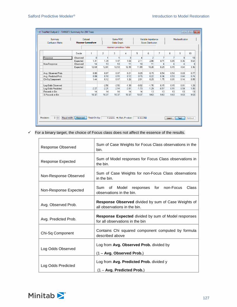
Salford Predictive Modeler® Introduction to Model Restoration
127
✓ For a binary target, the choice of Focus class does not affect the essence of the results.
Response Observed Sum of Case Weights for Focus Class observations in the
bin.
Response Expected Sum of Model responses for Focus Class observations in
the bin.
Non-Response Observed Sum of Case Weights for non-Focus Class observations
in the bin.
Non-Response Expected Sum of Model responses for non-Focus Class
observations in the bin.
Avg. Observed Prob. Response Observed divided by sum of Case Weights of
all observations in the bin.
Avg. Predicted Prob. Response Expected divided by sum of Model responses
for all observations in the bin
Chi-Sq Component Contains Chi squared component computed by formula
described above
Log Odds Observed Log from Avg. Observed Prob. divided by
(1 – Avg. Observed Prob.)
Log Odds Predicted Log from Avg. Predicted Prob. divided y
(1 – Avg. Predicted Prob.)
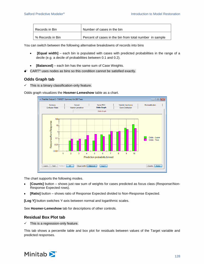
Salford Predictive Modeler® Introduction to Model Restoration
128
Records in Bin Number of cases in the bin
% Records in Bin Percent of cases in the bin from total number in sample
You can switch between the following alternative breakdowns of records into bins
• [Equal width] – each bin is populated with cases with predicted probabilities in the range of a
decile (e.g. a decile of probabilities between 0.1 and 0.2).
• [Balanced] – each bin has the same sum of Case Weights.
CART® uses nodes as bins so this condition cannot be satisfied exactly.
Odds Graph tab
✓ This is a binary classification-only feature.
Odds graph visualizes the Hosmer-Lemeshow table as a chart.
The chart supports the following modes.
[Counts] button – shows just raw sum of weights for cases predicted as focus class (Response\Non-Response Expected rows).
[Ratio] button – shows ratio of Response Expected divided to Non-Response Expected.
[Log Y] button switches Y-axis between normal and logarithmic scales.
See Hosmer-Lemeshow tab for descriptions of other controls.
Residual Box Plot tab
✓ This is a regression-only feature.
This tab shows a percentile table and box plot for residuals between values of the Target variable and
predicted responses.
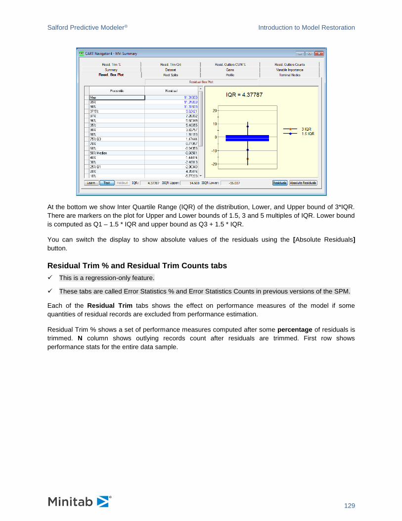
Salford Predictive Modeler® Introduction to Model Restoration
129
At the bottom we show Inter Quartile Range (IQR) of the distribution, Lower, and Upper bound of 3*IQR.
There are markers on the plot for Upper and Lower bounds of 1.5, 3 and 5 multiples of IQR. Lower bound
is computed as Q1 – 1.5 * IQR and upper bound as Q3 + 1.5 * IQR.
You can switch the display to show absolute values of the residuals using the [Absolute Residuals]
button.
Residual Trim % and Residual Trim Counts tabs
✓ This is a regression-only feature.
✓ These tabs are called Error Statistics % and Error Statistics Counts in previous versions of the SPM.
Each of the Residual Trim tabs shows the effect on performance measures of the model if some
quantities of residual records are excluded from performance estimation.
Residual Trim % shows a set of performance measures computed after some percentage of residuals is
trimmed. N column shows outlying records count after residuals are trimmed. First row shows
performance stats for the entire data sample.
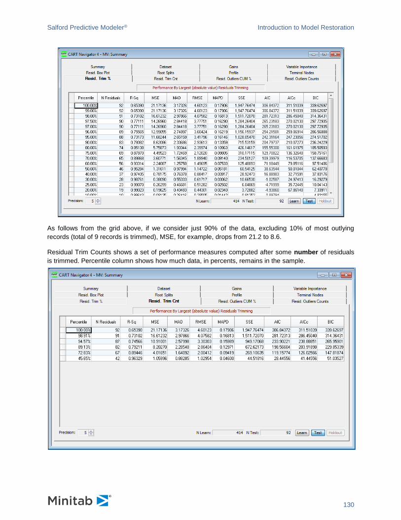
Salford Predictive Modeler® Introduction to Model Restoration
130
As follows from the grid above, if we consider just 90% of the data, excluding 10% of most outlying
records (total of 9 records is trimmed), MSE, for example, drops from 21.2 to 8.6.
Residual Trim Counts shows a set of performance measures computed after some number of residuals
is trimmed. Percentile column shows how much data, in percents, remains in the sample.

Salford Predictive Modeler® Introduction to Model Restoration
131
Residual Outliers % and Residual Outliers Counts tabs
✓ This is a regression-only feature.
✓ These tabs are called Error Outliers % and Error Outliers Counts in previous versions of SPM.
Each of the Residual Outliers tabs shows the effect on performance measures of the model if some
quantities of outlier records are excluded from performance estimation.
Residual Outlier CUM % tab shows for each performance measure a percentage of performance
measure value that is attributed to specific percent of outliers. N column shows number of outlying
records for each percentage of outliers.
As follows from the grid above, removing 1 record (1 percent) of outlying records will reduce MSE by
22%.
Residual Outliers Counts tab shows for each performance measure a percentage that is attributed to
specific count of outliers. %Residuals column shows the percentage of outlying records for each
number of residuals.
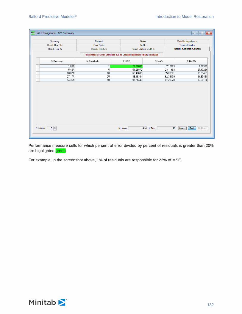
Salford Predictive Modeler® Introduction to Model Restoration
132
Performance measure cells for which percent of error divided by percent of residuals is greater than 20%
are highlighted green.
For example, in the screenshot above, 1% of residuals are responsible for 22% of MSE.