Introducing the R languageStatistical analysis made easy

Finlay ThompsonDragonfly Ltd.

Wellington Perl Mongers9 March 2009

Outline

1 Introducting RR is a tool for statistical analysisSome historyPackaged for your favourite distributionKind of like perl reallyActually quite different from perl

2 Looking at some iostat dataLoading the data into a frameUnderstanding through plotsTesting theories

R is a tool for statistical analysisIntroducing R

• Programming language for doing statisticalanalysis

• Excellent graphing and plotting routines,outputs SVG, PNG, PDF, etc..

• Hundreds of sophisticated algorithmscontributed via package system

• Plays the same role as SAS, S-Plus,Matlab, or SciPy

Some historyIntroducing R

• Project started by Ross Ihaka and RobertGentleman at Auckland University in 1993.

• Ross explains that he was experimentingwith Lisp, Scheme, and statisticalcomputing.

• Designed to be compatible with S, aproprietary statistical computing package.

R is free softwareIntroducing R

• In 1995 released with a GPL license.• Explosive growth in development,

with dozens of contributors.• Organized by the non-for-profit R

Foundation for statistical computing.

Large community of usersIntroducing R

• Intel Capital estimate over 1 million users.• CRAN - Comprehensive R Archive Network.• 70 mirrors in 33 different countries.• http://cran.stat.auckland.ac.nz/

• Heaps of contributed packages, all easily installed.• Corporate support available from Revolution Computinghttp://www.revolution-computing.com/

• Revolution estimate that there are over 2 million users.

Packaged for UbuntuIntroducing R

• Super easy to install on Ubuntu and Debiansudo aptitude install r-base-core r-recommended

• You can get the bleeding edge from:deb http://cran.stat.auckland.ac.nz/bin/linux/ubuntu karmic/

• approx 140 contributed packaged:

$ aptitude search r-cranp r-cran-abind - GNU R abind multi-dimensional array combinp r-cran-acepack - GNU R package for regression transformatiop r-cran-adapt - GNU R package providing multidimentional ip r-cran-amelia - GNU R package supporting multiple imputatip r-cran-bayesm - GNU R package for Bayesian inferencei A r-cran-bitops - GNU R package implementing bitwise operatii A r-cran-boot - GNU R package for bootstrapping functionsp r-cran-cairodevice - GNU R Cairo/Gtk2 device driver packagep r-cran-car - GNU R Companion to Applied Regression by Ji A r-cran-catools - GNU R package providing various utility fui r-cran-chron - GNU R package for chronologically orderedi A r-cran-cluster - GNU R package for cluster analysis by Rousi r-cran-coda - Output analysis and diagnostics for MCMC si A r-cran-codetools - GNU R package providing code analysis toolp r-cran-colorspace - GNU R Color Space Manipulationp r-cran-combinat - GNU R package with utilities for combinatop r-cran-date - GNU R package for date handlingp r-cran-dbi - GNU R package providing a generic database

Installing a packageIntroducing R

• Also possible to install packages using R, which compiles directlyfrom CRAN.

> install.packages(’afc’)trying URL ’http://cran.stat.auckland.ac.nz/src/contrib/afc_1.03.tar.gz’Content type ’application/x-gzip’ length 23469 bytes (22 Kb)opened URL==================================================downloaded 22 Kb

* Installing *source* package a f c ...

** R

** data

** preparing package for lazy loading

** help

*** installing help indices>>> Building/Updating help pages for package ’afc’

Formats: text html latex exampleafc-package text html latexafc text html latex exampleafc.cc text html latex exampleafc.ce text html latex example... cut some lines ...cnrm.nino34.mp text html latexrank.ensembles text html latex example

** building package indices ...

* DONE (afc)

The downloaded packages are in/tmp/RtmpXCB1I4/downloaded_packages

Kind of like perl reallyIntroducing R

• An open source, interpreted programming language.• Huge, well designed package archive CRAN.• Stable core system, with millions of users.• Weird tacked on support for object oriented programming.• Excellent syntax, with lots of $, @, and <-

1 apply_time <- function(datestring, lat, long, suffix){2 datetime <- strptime(datestring, ’%Y-%m-%d %H:%M:%S’)3 year <- datetime$year + 19004 mon <- datetime$mon + 15 day <- datetime$mday6 hour <- datetime$hour7 min <- datetime$min8 sec <- datetime$sec9 time <- hour + min/60 + sec/(60*60)

10 }

Actually quite different from perlIntroducing R

Pass by value semantics

• Easy to write memory inefficient programs.• Need to think carefully about memory usage.

Everything is an array

• The basic data type is an array.• All functions map over arrays.• Can be character, numeric, factor, etc

Loading the data into a frameiostat data

iostat collects disk usage information

• Thanks to Mark Kirkwood for providing a few days worth of iostatdata from a busy production computer.

• iostat sampled eleven statistics from two disks, every second.

Linux 2.6.26-2-amd64 (computer2) 03/02/10 _x86_64_

Time: 09:54:36Device: rrqm/s wrqm/s r/s w/s rMB/s wMB/s avgrq-sz avgqu-sz await svctm %utilsda 2.68 40.24 6.96 10.19 0.34 0.20 65.13 0.06 3.45 4.37 7.50sdb 2.66 40.32 6.88 10.39 0.33 0.22 65.45 0.56 32.39 4.04 6.98

Time: 09:54:37Device: rrqm/s wrqm/s r/s w/s rMB/s wMB/s avgrq-sz avgqu-sz await svctm %utilsda 0.00 54.55 4.04 9.09 0.03 0.26 45.54 0.08 6.15 5.54 7.27sdb 0.00 54.55 3.03 9.09 0.02 0.26 47.33 0.10 8.00 7.33 8.89

Loading the data into a frameiostat data

Use a perl script to flatten the data

Because this is a perl meeting, I used a perl script to flatten the datainto a simple csv type format.

1 #!/usr/bin/perl -nl2 next if /Linux/; # Skip first line3 next if /ˆ\s*$/; # Skip blank lines4 # Write header5 if (/ˆDevice:/) {6 print join ",", (’Time:’, split /\s+/) unless $header++;7 next;8 }9 # save time

10 if (/ˆTime:\s+(.*)$/) {11 $time = $1;12 next;13 }14 # Write line15 print join ",", $time, split /\s+/;

Loading the data into a frameiostat data

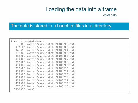
The data is stored in a bunch of files in a directory

$ wc -l iostat/raw/*16362 iostat/raw/iostat-20100202.out144462 iostat/raw/iostat-20100203.out143692 iostat/raw/iostat-20100204.out414002 iostat/raw/iostat-20100205.out414002 iostat/raw/iostat-20100206.out414002 iostat/raw/iostat-20100207.out414002 iostat/raw/iostat-20100208.out414002 iostat/raw/iostat-20100209.out414002 iostat/raw/iostat-20100210.out414002 iostat/raw/iostat-20100211.out414002 iostat/raw/iostat-20100212.out414002 iostat/raw/iostat-20100213.out414002 iostat/raw/iostat-20100214.out414002 iostat/raw/iostat-20100215.out275472 iostat/raw/iostat-20100216.out

5134010 total

Loading the data into a frameiostat data

We can load data into R using the perl script

1 days <- 20100203:201002162

3 iostat <- c()4 for (day in days[4]) {5 file <- pipe(sprintf(’perl load.pl raw/iostat-%d.out’, day))6 d <- read.csv(file)7 iostat <- rbind(iostat, cbind(day, d))8 }

Loading the data into a frameiostat data

Interactively

$ RR version 2.9.2 (2009-08-24)Copyright (C) 2009 The R Foundation for Statistical ComputingISBN 3-900051-07-0

> days <- 20100203:20100216> days[1] 20100203 20100204 20100205 20100206 20100207 20100208 20100209 20100210[9] 20100211 20100212 20100213 20100214 20100215 20100216

>

Loading the data into a frameiostat data

Interactively check this out

> iostat <- c()> for (day in days[4]) {+ file <- pipe(sprintf(’perl load.pl raw/iostat-%d.out’, day))+ d <- read.csv(file)+ iostat <- rbind(iostat, cbind(day, d))+ }> str(iostat)’data.frame’: 165600 obs. of 14 variables:$ day : int 20100206 20100206 20100206 20100206 20100206 20100206 20100206 20100206 20100206 20100206 ...$ Time. : Factor w/ 82797 levels "00:31:01","00:31:02",..: 1 1 2 2 3 3 4 4 5 5 ...$ Device. : Factor w/ 2 levels "sda","sdb": 1 2 1 2 1 2 1 2 1 2 ...$ rrqm.s : num 2.71 2.69 0 0 0 0 0 0 0 0 ...$ wrqm.s : num 40.5 40.59 9.09 8.08 873 ...$ r.s : num 7.09 7.01 1.01 0 0 0 0 0 0 0 ...$ w.s : num 10.2 10.4 20.2 18.2 84 ...$ rMB.s : num 0.35 0.34 0.01 0 0 0 0 0 0 0 ...$ wMB.s : num 0.2 0.22 0.12 0.11 3.76 3.76 0.31 0.31 0.1 0.1 ...$ avgrq.sz: num 65.1 65.4 12.2 12 91.7 ...$ avgqu.sz: num 0.08 0 0.17 0.13 5.73 5.43 0.04 0.04 0.08 0.06 ...$ await : num 4.58 32.22 8.95 7.11 68.19 ...$ svctm : num 4.36 4.03 5.71 5.11 4.95 4.29 5.6 7.2 6.67 5 ...$ X.util : num 7.56 7.03 12.12 9.29 41.6 ...

>

Loading the data into a frameiostat data

Thin the data by sampling 3500 from each file

1 iostat <- c()2 for (day in days) {3 file <- pipe(sprintf(’perl load.pl raw/iostat-%d.out’, day))4 d <- read.csv(file)5 d <- d[sort(sample(1:dim(d)[1], 3500)),]6 iostat <- rbind(iostat, cbind(day, d))7 }

The function sample takes an array and sample a given number ofelements from it. In this case we are sampling from the first index ofthe data frame d.

Loading the data into a frameiostat data

Now we can cast the parse the times into time objects

1 library(chron)2 iostat$times <- with(iostat, times(Time.))

The function with is a local scoping tool, simplifying expressions.The library chron has useful data types for dealing with dates andtimes. Like perl, there are a number of date/time libraries.

Understanding through plotsiostat data

Reads per second through the day

1 with(iostat,2 plot(x=times, y=r.s, type=’p’, pch=16, cex=0.4)3 )

Understanding through plotsiostat data

Reads per second through the day

1 with(iostat,2 plot(x=times, y=r.s, type=’p’, pch=16, cex=0.4, log=’y’)3 )

Understanding through plotsiostat data

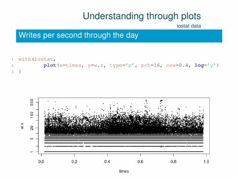
Writes per second through the day

1 with(iostat,2 plot(x=times, y=w.s, type=’p’, pch=16, cex=0.4, log=’y’)3 )

Understanding through plotsiostat data

Writes per second through the day, on first disk

1 with(iostat[iostat$Device. == ’sda’,],2 plot(x=times, y=w.s, type=’p’, pch=16, cex=0.4, log=’y’)3 )

Understanding through plotsiostat data

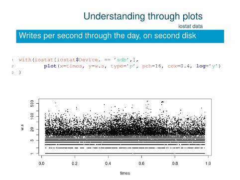
Writes per second through the day, on second disk

1 with(iostat[iostat$Device. == ’sdb’,],2 plot(x=times, y=w.s, type=’p’, pch=16, cex=0.4, log=’y’)3 )

Understanding through plotsiostat data

Looking at the density

1 sda <- iostat$Device. == ’sda’2 sdb <- iostat$Device. == ’sdb’3 with(iostat[sda,], plot(density(log(w.s)),label=""))4 with(iostat[sdb,], lines(density(log(w.s)), col="blue"))

Understanding through plotsiostat data

Correlations

1 with(iostat, pairs(˜ avgrq.sz + await + avgqu.sz))2 with(iostat, pairs(˜ avgqu.sz + r.s + w.s))

Testing theoriesiostat data

Writes per second versus average request size

1 with(iostat[iostat$w.s>0 & iostat$avgqu.sz > 0,],2 plot(log(avgqu.sz), log(w.s))3 )

Testing theoriesiostat data

Writes per second versus average request size

1 with(iostat[iostat$w.s>0 & iostat$avgqu.sz > 0,],2 points(supsmu(log(avgqu.sz), log(w.s)),type=’l’, col=’red’)3 )

Testing theoriesiostat data

> m <- lm(I(log(avgqu.sz)) ˜ I(log(w.s)),data=iostat[iostat$w.s>0 & iostat$avgqu.sz > 0,])

> summary(m)

Call:lm(formula = I(log(avgqu.sz)) ˜ I(log(w.s)), data = iostat[iostat$w.s >

0 & iostat$avgqu.sz > 0, ])

Residuals:Min 1Q Median 3Q Max

-2.9405 -0.4823 -0.1745 0.3059 6.0819

Coefficients:Estimate Std. Error t value Pr(>|t|)

(Intercept) -5.165586 0.011770 -438.9 <2e-16 ***I(log(w.s)) 1.456640 0.004682 311.1 <2e-16 ***---Signif. codes: 0 *** 0.001 ** 0.01 * 0.05 . 0.1 1

Residual standard error: 0.8095 on 33225 degrees of freedomMultiple R-squared: 0.7445, Adjusted R-squared: 0.7445F-statistic: 9.68e+04 on 1 and 33225 DF, p-value: < 2.2e-16