introduction a freefem++` · freefem++ est un solveur permettant de r esoudre les equations aux d...

Introduction a FreeFem++J.Morice

Laboratoire Jacques-Louis Lions

Universite Pierre et Marie Curie

Paris, France

avec O. Pironneau, F. Hecht

http://www.freefem.org mailto:[email protected]

Finance par l’Agence National de La Recherche(ANR) ANR-07-CIS7-002-01

http://www.freefem.org/ff2a3/ http://www-anr-ci.cea.fr/

FreeFem++ Cours M2, dec. 2009 1

http://www.freefem.org

mailto:[email protected]

http://www.freefem.org/ff2a3/

http://www-anr-ci.cea.fr/

PLAN

– Introduction Freefem++

– Element Syntaxe

– Formulation Variationnelle et EF

– Generation de maillage 2D

– Examples :

– Equation de Poisson avec condition de Neumann et condition de Dirichlet

– Equation de Poisson avec systeme matricielle

– Adaptation de Maillage avec indication d’erreur

– Probleme de Stokes 3D

– Generation de maillage 3D


Introduction

FreeFem++ est un solveur permettant de resoudre les equations aux derivees

partielles (PDE) en 2d et 3d.

Methode employe : Methode d’elements finis. EF : P0, P1, P2,

Raviart-Thomas, P1 diconstinue,

FreeFem++ est un logiciel sous licence LGPL. Il fonctionne sous Mac, Unix

et Window. Algorithme // avec MPI.


The main characteristics of FreeFem++ I/II (2D)

– Wide range of finite elements : linear (2d,3d) (P1) and quadratic Lagran-

gian (2d,3d) elements (P2), discontinuous P1 and Raviart-Thomas elements

(2d,3d), 3d Edge element , vectorial element, mini-element( 2d, 3d), ...

– Automatic interpolation of data from a mesh to an other one, so a finite

element function is view as a function of (x, y, z) or as an array.

– Definition of the problem (complex or real value) with the variational form

with access to the vectors and the matrix if needed

– Discontinuous Galerkin formulation (only 2d to day).


The main characteristics of FreeFem++ II/II (2D)

– Analytic description of boundaries, with specification by the user of the

intersection of boundaries in 2d.

– Automatic mesh generator, based on the Delaunay-Voronoi algorithm. (2d,3d)

– load and save Mesh, solution

– Mesh adaptation based on metric, possibly anisotropic, with optional auto-

matic computation of the metric from the Hessian of a solution.

– LU, Cholesky, Crout, CG, GMRES, UMFPack, SuperLU, MUMPS, ... sparse

linear solver ; eigenvalue and eigenvector computation with ARPACK.

– Online graphics, C++ like syntax.

– Link with other soft : modulef, emc2, medit, gnuplot, tetgen, superlu,

mumps ...

– Dynamic linking to add functonality.

– Wide range of of examples : Navier-Stokes 3d, elasticity 3d, fluid structure,

eigenvalue problem, Schwarz’ domain decomposition algorithm, residual er-

ror indicator, ...


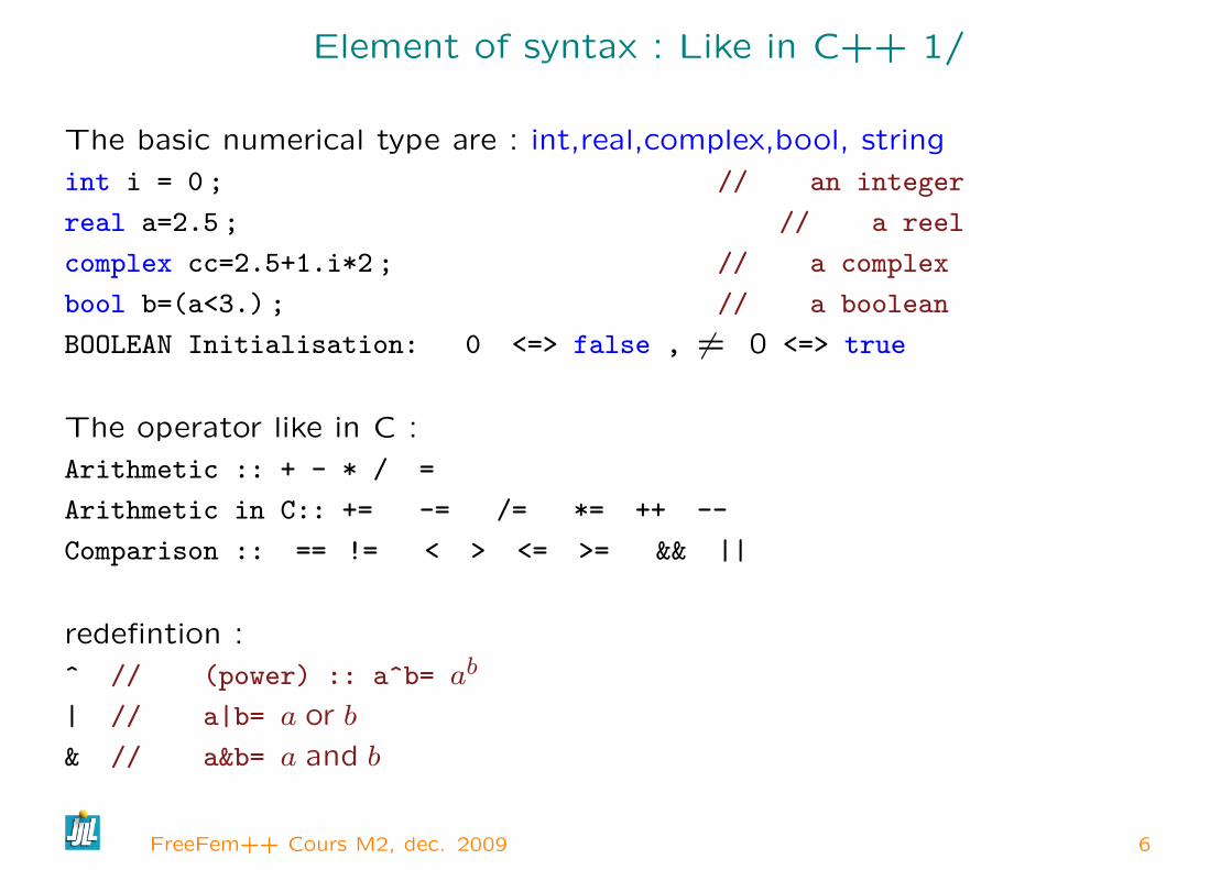
Element of syntax : Like in C++ 1/

The basic numerical type are : int,real,complex,bool, string

int i = 0 ; // an integer

real a=2.5 ; // a reel

complex cc=2.5+1.i*2 ; // a complex

bool b=(a<3.) ; // a boolean

BOOLEAN Initialisation: 0 <=> false , 6= 0 <=> true

The operator like in C :

Arithmetic :: + - * / =

Arithmetic in C:: += -= /= *= ++ --

Comparison :: == != < > <= >= && ||

redefintion :

^ // (power) :: a^b= ab

| // a|b= a or b

& // a&b= a and b


Element of syntax : Like in C++ 2

// Automatic cast for numerical value : bool, int, reel, complex

func f=x+y ; // a formal line function

func real g(int i, real a) ..... ; return i+a ;

// Loops

for (int i=0 ;i<n ;i++) ... ;

if ( <bool exp> ) ... ; else ... ; ;

while ( <bool exp> ) ... ;

break continue key words

// The scoop of a variable the current block :

int a=1 ; // a block

cout << a << endl ; // error the variable a not existe here.

lots of math function : exp, log, tan, ...


Element of syntax : 4/4

Les Entrees / sorties comme en c++

Ecran : : cout, cin, ...

Pour ouvrir un fichier en lecture :ifstream name(nom_fichier) ;

Pour ouvrir un fichier en ecriture :ofstream name(nom_fichier) ;

Lire / ecriture dans un fichier >> /<<

ofstream gnu("plot.gp") ;

gnu.precision(14) ; // gnu.fixed() ; gnu.scientific() ; (Section 4.10

doc FreeFem++)

for (int i=0 ;i<n ;i++)

gnu << x[i] << " " << y[i] << endl ;


Element of syntax 3 : Array, Tabular and Matrix

real[int] Realarray(10) ; // a real array of 10 value

int[int] IntArray(20) ; // an integer array of 20 value

real[int,int] T(30,30) // a Tabular of size 30 × 30

T(2,3) = 5.0 ;

⇒ Pb : Tabular T ' Full Matrix

// Sparse Matrix (all non zero value are not storage)

matrix M1=T ; // Matrix of size 30 × 30 with value of Tabular T

// Block matrix

matrix M2= [ [A, 0, B ],

[ 0, A, B ],

[B’, B’, M] ] ; // where B’ is the transpose of matrix B.


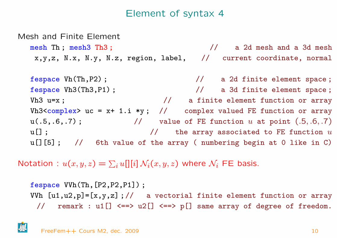
Element of syntax 4

Mesh and Finite Element

mesh Th ; mesh3 Th3 ; // a 2d mesh and a 3d mesh

x,y,z, N.x, N.y, N.z, region, label, // current coordinate, normal

fespace Vh(Th,P2) ; // a 2d finite element space ;

fespace Vh3(Th3,P1) ; // a 3d finite element space ;

Vh3 u=x ; // a finite element function or array

Vh3<complex> uc = x+ 1.i *y ; // complex valued FE function or array

u(.5,.6,.7) ; // value of FE function u at point (.5, .6, .7)

u[] ; // the array associated to FE function u

u[][5] ; // 6th value of the array ( numbering begin at 0 like in C)

Notation : u(x, y, z) =∑i u[][i]Ni(x, y, z) where Ni FE basis.

fespace VVh(Th,[P2,P2,P1]) ;

VVh [u1,u2,p]=[x,y,z] ;// a vectorial finite element function or array

// remark : u1[] <==> u2[] <==> p[] same array of degree of freedom.


probleme variationnel

Definition du probleme

Vh u,v ;

problem pbname(u,v,solver=CG,eps=1.e-6)= a(u,v) - l(v) + (conditions aux

limites) ; /

pbname ; // resolution du probleme variationnel

solver= CG, GMRES, UMFPACK, Crout, LU, Cholesky


probleme modele On va considerer le problem definition dans la section Weak

form and Boundary Condition de la documentation FreeFem++.

The problem is : Find u a real function defined on domain Ω of Rd (d = 2,3)

such that

−∇.(κ∇u) = f, in Ω,

au+ κ∂u

∂n= b on Γr,

u = g on Γd

Varitionnal Form Find u ∈ Vg = v ∈ H1(Ω)/v = g on Γd such that∫Ωκ∇v.∇u dω +

∫Γrauv dγ =

∫Ωfv dω +

∫Γrbv dγ, ∀v ∈ V0 (1)

where V0 = v ∈ H1(Ω)/v = 0 on Γd


2D case

Find u ∈ Vg = v ∈ H1(Ω)/v = g on Γd such that∫Ωκ∇v.∇u dω +

∫Γrauv dγ =

∫Ωfv dω +

∫Γrbv dγ, ∀v ∈ V0 (2)

where V0 = v ∈ H1(Ω)/v = 0 on Γd

problem Pw(u,v) =

int2d(Th)( kappa*( dx(u)*dx(u) + dy(u)*dy(u)) ) //∫Ω κ∇v.∇u dω

+ int1d(Th,gr)( a * u*v ) //∫Γr auv dγ

- int2d(Th)(f*v) //∫Ω fv dω

- int1d(Th,gr)( b * v ) //∫Γr bv dγ

+ on(gd)(u= g) ; // u = g on Γd

Also

intalledge(Th) // integration over the all edges in the mesh


3D case

∫Ωκ∇v.∇u dω +

∫Γrauv dγ =

∫Ωfv dω +

∫Γrbv dγ, ∀v ∈ V0 (3)

where V0 = v ∈ H1(Ω)/v = 0 on Γdmacro Grad(u) [dx(u),dy(u),dz(u) ] // EOM : definition of the 3d Grad

macro

problem Pw(u,v) =

int3d(Th)( kappa*( Grad(u)’*Grad(v) ) ) //∫Ω κ∇v.∇u dω

+ int2d(Th,gr)( a * u*v ) //∫Γr auv dγ

- int3d(Th)(f*v) //∫Ω fv dω

- int2d(Th,gr)( b * v ) //∫Γr bv dγ

+ on(gd)(u= g) ; // u = g on Γd


Mesh 1

mesh Th ; mesh3 Th3 ; // a 2d mesh and a 3d mesh

First a 10× 10 grid mesh of unit square ]0,1[2mesh Th1 = square(10,10) ; // boundary label:int[int] re=[1,1, 2,1, 3,1, 4,1] // 1 -> 1 bottom, 2 -> 1 right,

// 3->1 top, 4->1 leftTh1=change(Th1,refe=re) ; // boundary label is 1plot(Th1,wait=1) ;

Get a extern mesh

mesh Th2("april-fish.msh") ;

mesh Th2=readmesh("april-fish.msh") ;


Mesh 2 : parametrized boundary

A domain is defined as being on the left (resp right) of its parameterized

boundary

Γj = (x, y) | x = ϕx(t), y = ϕy(t), t0 ≤ t ≤ t1

border GammaJ(t=t0,t1)x=varphiX(t) ;y=varphiY(t) ;label=1 ; ;

In the figure, the domain lie on the shaded area.

G j

t = t 0

t = t 1( x = j x ( t ) , y = j y ( t ) )

( d j x ( t ) / d t , d j y ( t ) / d t )( x = t , y = t ) ( x = t , y = - t )t = t 0

t = t 1

t = t 1

t = t 0


Mesh 3 : triangulate a two dimension domain

The general expression to define a triangulation with buildmesh is

mesh MeshName = buildmesh(Γ1(m1) + · · ·+ ΓJ(mj), OptionalParameter

);

where mj are positive or negative numbers to indicate how may point should

be put on Γj, Γ = ∪Jj=1ΓJ, and the optional parameter are

fixeborder=<bool value> , to say if the mesh generator can change the boun-

dary mesh or not (by default the boundary mesh can change).

⇒ periodic boundary problem and gluing mesh.


Mesh 4 ; Example

first a mesh with a hole

1: border a(t=0,2*pi) x=cos(t) ; y=sin(t) ;label=1 ;2: border b(t=0,2*pi) x=0.3+0.3*cos(t) ; y=0.3*sin(t) ;label=2 ;3: plot(a(50)+b(+30)) ; // to see a plot of the border mesh4: mesh Thwithouthole= buildmesh(a(50)+b(+30)) ;5: mesh Thwithhole = buildmesh(a(50)+b(-30)) ;6: plot(Thwithouthole,wait=1,ps="Thwithouthole.eps") ;7: plot(Thwithhole,wait=1,ps="Thwithhole.eps") ;


Mesh 5 triangulate a two dimension domain

second a L shape domain ]0,1[2\[12,1[2

border a(t=0,1.0)x=t ; y=0 ; label=1 ; ;border b(t=0,0.5)x=1 ; y=t ; label=2 ; ;border c(t=0,0.5)x=1-t ; y=0.5 ;label=3 ; ;border d(t=0.5,1)x=0.5 ; y=t ; label=4 ; ;border e(t=0.5,1)x=1-t ; y=1 ; label=5 ; ;border f(t=0.0,1)x=0 ; y=1-t ;label=6 ; ;plot(a(6) + b(4) + c(4) +d(4) + e(4) + f(6),wait=1) ; // to see the 6 bordersmesh Th2 = buildmesh (a(6) + b(4) + c(4) +d(4) + e(4) + f(6)) ;


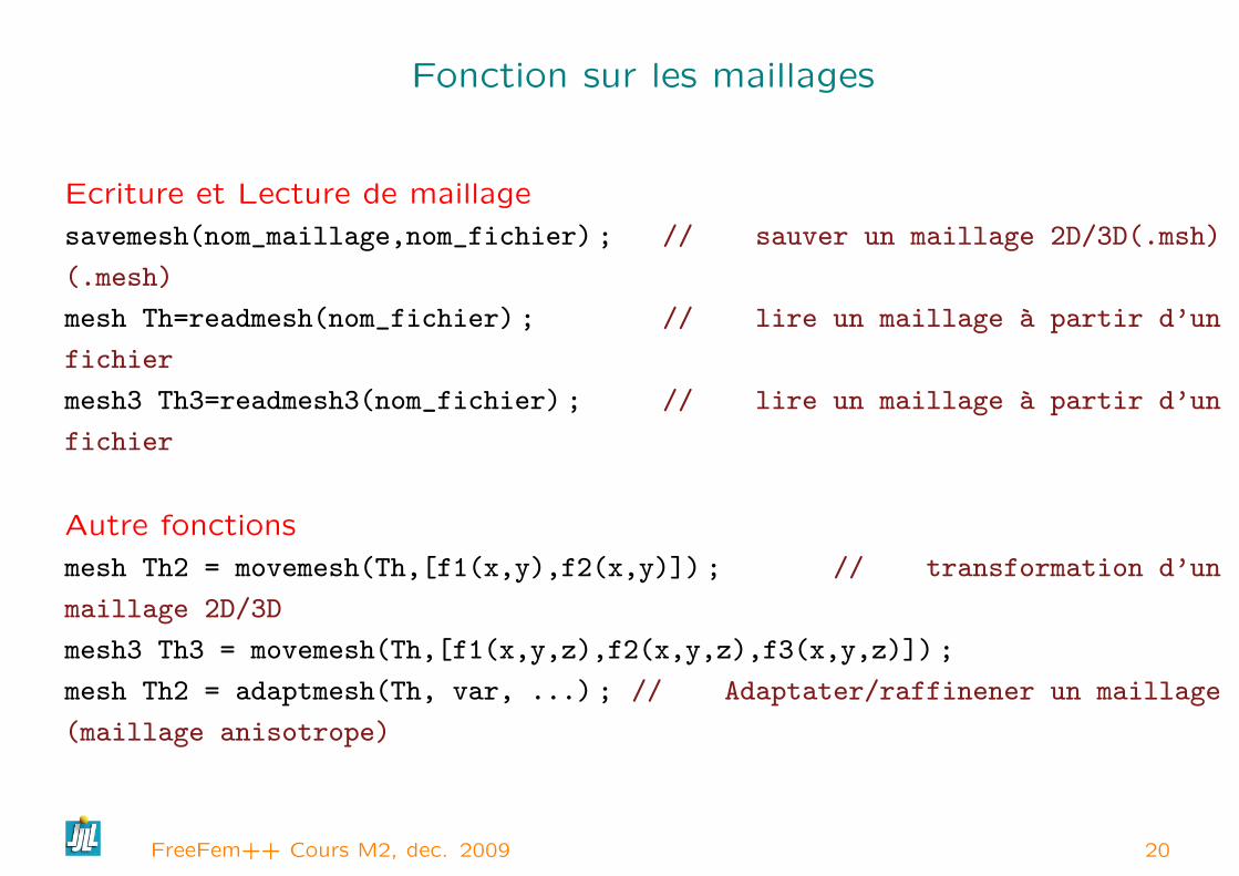
Fonction sur les maillages

Ecriture et Lecture de maillage

savemesh(nom_maillage,nom_fichier) ; // sauver un maillage 2D/3D(.msh)

(.mesh)

mesh Th=readmesh(nom_fichier) ; // lire un maillage a partir d’un

fichier

mesh3 Th3=readmesh3(nom_fichier) ; // lire un maillage a partir d’un

fichier

Autre fonctions

mesh Th2 = movemesh(Th,[f1(x,y),f2(x,y)]) ; // transformation d’un

maillage 2D/3D

mesh3 Th3 = movemesh(Th,[f1(x,y,z),f2(x,y,z),f3(x,y,z)]) ;

mesh Th2 = adaptmesh(Th, var, ...) ; // Adaptater/raffinener un maillage

(maillage anisotrope)


vizualisations des resultats

– Directement avec Freefem++ Afficher des maillages, solutions scalaires et

vectorielles

– Fonction plot :

plot(var1,[var2,var3],...[liste d’options]) ;

// options

wait=true/false,

value=true/false, :: isolines and arrow vector

fill=true/false, :: colloriage du domaine

ps="nom_fichier",...

Les raccourci de la fenetre sont obtenue en ?

– Fonction medit :

medit("sol1 sol2 ",Th,sca,[Vx,Vy],wait=1,save="resultats.sol", order=1) ;

– Exporter vers un autre logiciel Gnuplot, Medit (savemesh, savesol), Paraview,

...


Laplace equation, weak form

Let a domain Ω with a partition of ∂Ω in Γ2,Γe.

Find u a solution in such that :

−∆u = 1 in Ω, u = 2 on Γ2,∂u

∂~n= 0 on Γe (4)

Denote Vg = v ∈ H1(Ω)/v|Γ2= g .

The Basic variationnal formulation with is : find u ∈ V2(Ω) , such that∫Ω∇u.∇v =

∫Ω

1v+∫

Γ

∂u

∂nv, ∀v ∈ V0(Ω) (5)


Laplace equation in FreeFem++

The finite element method is just : replace Vg with a finite element space,

and the FreeFem++ code :

fespace Xh(Th,P1) ; // define the P1 EF space

Xh u,v ;

solve laplace(u,v,solver=CG) =

int2d(Th)( dx(u)*dx(v)+dy(u)*dy(v) ) - int2d(Th) ( 1*v)

+ on(2,u=2) ; // int on γ2

plot(u,fill=1,wait=1,value=0) ;


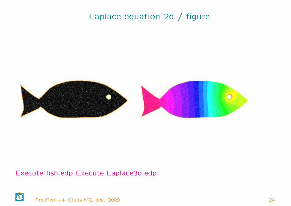
Laplace equation 2d / figure

Execute fish.edp Execute Laplace3d.edp


Matrix and vector

The 2d FreeFem++ code :

fespace Xh(Th,P2) ; // define the P2 EF space

Xh u,v ;

varf vlaplace(u,v,solver=CG) =

int2d(Th)( dx(u)*dx(v)+dy(v)*dy(v) ) + int2d(Th) ( 1*v) //

vlaplace(u,v) = a(u,v)+b(v)

+ on(2,u=2) ; // on γ2

matrix A= vlaplace(Xh,Xh,solver=CG) ; // bilinear part

real[int] b=vlaplace(0,Vh) ; // // linear part

u[] = A^-1*b ;

Execute fish-MatrixVector.edp


Remark on varf

The functions appearing in the variational form are formal and local to thevarf definition, the only important think in the order in the parameter list,like invarf vb1([u1,u2],[q]) = int2d(Th)( (dy(u1)+dy(u2)) *q)) + int2d(Th)(1*q) ;

varf vb2([v1,v2],[p]) = int2d(Th)( (dy(v1)+dy(v2)) *p)) + int2d(Th)(1*p) ;

To build matrix A from the bilinear part the the variational form a of typevarf do simplymatrix B1 = vb1(Vh,Wh [, ... optional named param ] ) ;

matrix<complex> C1 = vb1(Vh,Wh [, ... optional named param ] ) ;

// where

// the fespace have the correct number of component

// Vh is "fespace" for the unknown fields with 2 components

// ex fespace Vh(Th,[P2,P2]) ; or fespace Vh(Th,RT0) ;

// Wh is "fespace" for the test fields with 1 component

To build matrix a vector, the u1 = u2 = 0.real[int] b = vb2(0,Wh) ;

complex[int] c = vb2(0,Wh) ;


The boundary condition terms

– An ”on” scalar form (for Dirichlet ) : on(1, u = g )

The meaning is for all degree of freedom i of this associated boundary,

the diagonal term of the matrix aii = tgv with the terrible giant value tgv

(=1030 by default) and the right hand side b[i] = ”(Πhg)[i]” × tgv, where

the ”(Πhg)g[i]” is the boundary node value given by the interpolation of g.

– An ”on” vectorial form (for Dirichlet ) : on(1,u1=g1,u2=g2) If you have

vectorial finite element like RT0, the 2 components are coupled, and so you

have : b[i] = ”(Πh(g1, g2))[i]”× tgv, where Πh is the vectorial finite element

interpolant.

– a linear form on Γ (for Neumann in 2d )

-int1d(Th)( f*w) or -int1d(Th,3))( f*w)

– a bilinear form on Γ or Γ2 (for Robin in 2d)

int1d(Th)( K*v*w) or int1d(Th,2)( K*v*w).

– a linear form on Γ (for Neumann in 3d )

-int2d(Th)( f*w) or -int2d(Th,3))( f*w)

– a bilinear form on Γ or Γ2 (for Robin in 3d)

int2d(Th)( K*v*w) or int2d(Th,2)( K*v*w).


Laplace equation (mixted formulation) II/II

Now we solve −∆p = f on Ω and p = g on ∂Ω, with ~u = ∇p

so the problem becomes :

Find ~u, p a solution in a domain Ω such that :

−∇.~u = f, ~u−∇p = 0 in Ω, p = g on Γ = ∂Ω (6)

Mixted variationnal formulation

find ~u ∈ Hdiv(Ω), p ∈ L2(Ω) , such that

∫Ωq∇.~u+

∫Ωp∇.~v + ~u.~v =

∫Ω−fq +

∫Γg~v.~n, ∀(~v, q) ∈ Hdiv × L2


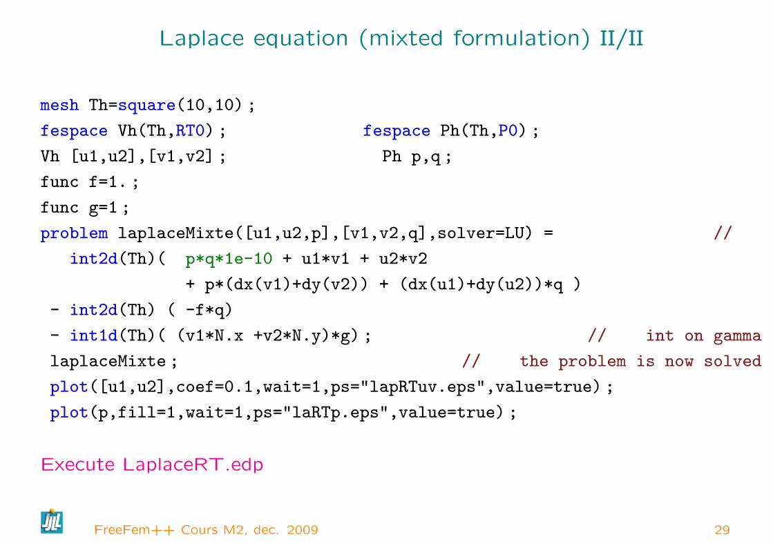
Laplace equation (mixted formulation) II/II

mesh Th=square(10,10) ;

fespace Vh(Th,RT0) ; fespace Ph(Th,P0) ;

Vh [u1,u2],[v1,v2] ; Ph p,q ;

func f=1. ;

func g=1 ;

problem laplaceMixte([u1,u2,p],[v1,v2,q],solver=LU) = //

int2d(Th)( p*q*1e-10 + u1*v1 + u2*v2

+ p*(dx(v1)+dy(v2)) + (dx(u1)+dy(u2))*q )

- int2d(Th) ( -f*q)

- int1d(Th)( (v1*N.x +v2*N.y)*g) ; // int on gamma

laplaceMixte ; // the problem is now solved

plot([u1,u2],coef=0.1,wait=1,ps="lapRTuv.eps",value=true) ;

plot(p,fill=1,wait=1,ps="laRTp.eps",value=true) ;

Execute LaplaceRT.edp


a corner singularity adaptation with metric

The domain is an L-shaped polygon Ω =]0,1[2\[12,1]2 and the PDE is

Find u ∈ H10(Ω) such that −∆u = 1 in Ω,

The solution has a singularity at the reentrant angle and we wish to capture

it numerically.

example of Mesh adaptation


FreeFem++ corner singularity program

border a(t=0,1.0)x=t ; y=0 ; label=1 ; ;border b(t=0,0.5)x=1 ; y=t ; label=2 ; ;border c(t=0,0.5)x=1-t ; y=0.5 ;label=3 ; ;border d(t=0.5,1)x=0.5 ; y=t ; label=4 ; ;border e(t=0.5,1)x=1-t ; y=1 ; label=5 ; ;border f(t=0.0,1)x=0 ; y=1-t ;label=6 ; ;

mesh Th = buildmesh (a(6) + b(4) + c(4) +d(4) + e(4) + f(6)) ;fespace Vh(Th,P1) ; Vh u,v ; real error=0.01 ;problem Problem1(u,v,solver=CG,eps=1.0e-6) =

int2d(Th)( dx(u)*dx(v) + dy(u)*dy(v)) - int2d(Th)( v)+ on(1,2,3,4,5,6,u=0) ;

int i ;for (i=0 ;i< 7 ;i++)Problem1 ; // solving the pde problemTh=adaptmesh(Th,u,err=error) ; // the adaptation with Hessian of uplot(Th,wait=1) ;u=u ;error = error/ (1000^(1./7.)) ;

;

Execute adapt.edp


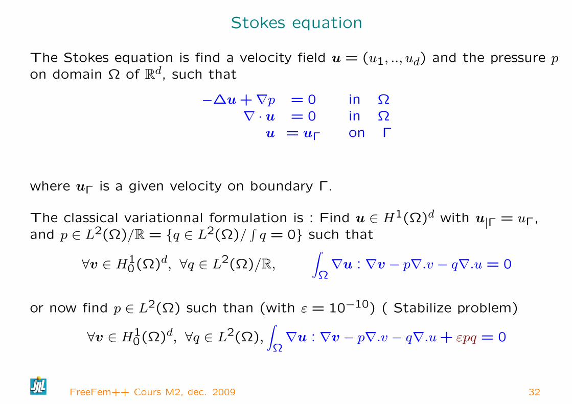
Stokes equation

The Stokes equation is find a velocity field u = (u1, .., ud) and the pressure pon domain Ω of Rd, such that

−∆u +∇p = 0 in Ω∇ · u = 0 in Ω

u = uΓ on Γ

where uΓ is a given velocity on boundary Γ.

The classical variationnal formulation is : Find u ∈ H1(Ω)d with u|Γ = uΓ,and p ∈ L2(Ω)/R = q ∈ L2(Ω)/

∫q = 0 such that

∀v ∈ H10(Ω)d, ∀q ∈ L2(Ω)/R,

∫Ω∇u : ∇v − p∇.v − q∇.u = 0

or now find p ∈ L2(Ω) such than (with ε = 10−10) ( Stabilize problem)

∀v ∈ H10(Ω)d, ∀q ∈ L2(Ω),

∫Ω∇u : ∇v − p∇.v − q∇.u+ εpq = 0


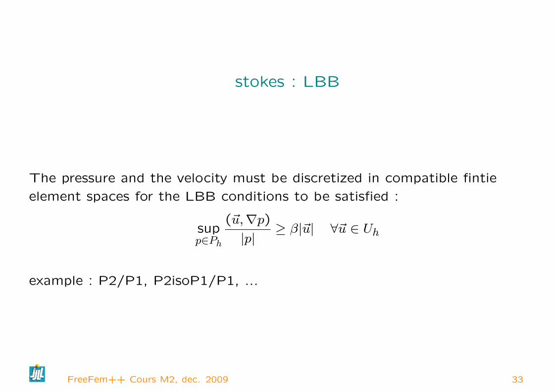
stokes : LBB

The pressure and the velocity must be discretized in compatible fintie

element spaces for the LBB conditions to be satisfied :

supp∈Ph

(~u,∇p)

|p|≥ β|~u| ∀~u ∈ Uh

example : P2/P1, P2isoP1/P1, ...


Stokes equation 3D in FreeFem++

... Build mesh .... Th (3d) T2d ( 2d)

fespace VVh(Th,[P2,P2,P2,P1]) ; // Taylor Hood Finite element.

macro Grad(u) [dx(u),dy(u),dz(u)] // EOM

macro div(u1,u2,u3) (dx(u1)+dy(u2)+dz(u3)) // EOM

varf vStokes([u1,u2,u3,p],[v1,v2,v3,q]) = int3d(Th)(

Grad(u1)’*Grad(v1) + Grad(u2)’*Grad(v2) + Grad(u3)’*Grad(v3)

- div(u1,u2,u3)*q - div(v1,v2,v3)*p + 1e-10*q*p )

+ on(1,u1=0,u2=0,u3=0) + on(2,u1=1,u2=0,u3=0) ;

matrix A=vStokes(VVh,VVh) ; set(A,solver=UMFPACK) ;

real[int] b= vStokes(0,VVh) ;

VVh [u1,u2,u3,p] ; u1[]= A^-1 * b ;

// 2d intersection of plot

fespace V2d(T2d,P2) ; // 2d finite element space ..

V2d ux= u1(x,0.5,y) ; V2d uz= u3(x,0.5,y) ; V2d p2= p(x,0.5,y) ;

plot([ux,uz],p2,cmm=" cut y = 0.5") ;

Execute Stokes3d.edp


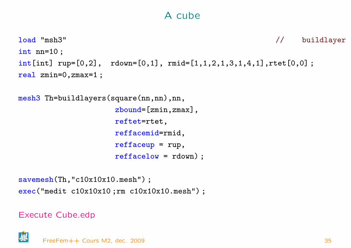
A cube

load "msh3" // buildlayer

int nn=10 ;

int[int] rup=[0,2], rdown=[0,1], rmid=[1,1,2,1,3,1,4,1],rtet[0,0] ;

real zmin=0,zmax=1 ;

mesh3 Th=buildlayers(square(nn,nn),nn,

zbound=[zmin,zmax],

reftet=rtet,

reffacemid=rmid,

reffaceup = rup,

reffacelow = rdown) ;

savemesh(Th,"c10x10x10.mesh") ;

exec("medit c10x10x10 ;rm c10x10x10.mesh") ;

Execute Cube.edp


3D layer mesh of a Lac

load "msh3"// buildlayer

load "medit"// buildlayer

int nn=5 ;

border cc(t=0,2*pi)x=cos(t) ;y=sin(t) ;label=1 ;

mesh Th2= buildmesh(cc(100)) ;

fespace Vh2(Th2,P2) ;

Vh2 ux,uz,p2 ;

int[int] rup=[0,2], rdown=[0,1], rmid=[1,1] ;

func zmin= 2-sqrt(4-(x*x+y*y)) ; func zmax= 2-sqrt(3.) ;

// we get nn*coef layers

mesh3 Th=buildlayers(Th2,nn,

coef= max((zmax-zmin)/zmax,1./nn),

zbound=[zmin,zmax],

reffacemid=rmid, reffaceup = rup,

reffacelow = rdown) ; // label def

medit("lac",Th) ;

Execute Lac.edp Execute 3d-leman.edp


sortie d’une matrice

matrix A= [[0, 1, 6 ],

[0, 0, 2 ],

[3, 0, 0 ]] ;

cout << A << endl ;

# Sparse Matrix (Morse)

# first line : n m (is symmetic) nbcoef

# after for each nonzero coefficient : i j ai j where (i, j) ∈ 1, ..., n × 1, ...,m

3 3 0 4

1 2 1

1 3 6

2 3 2

3 1 3


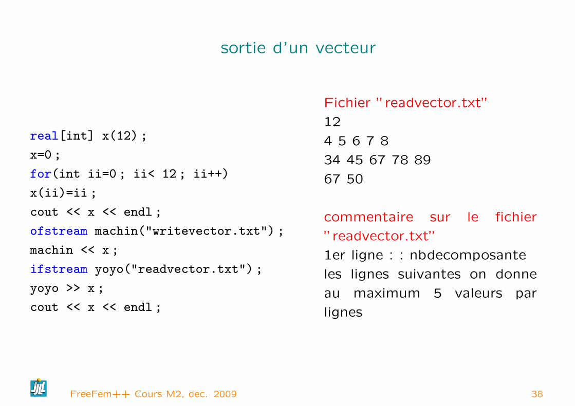
sortie d’un vecteur

real[int] x(12) ;

x=0 ;

for(int ii=0 ; ii< 12 ; ii++)

x(ii)=ii ;

cout << x << endl ;

ofstream machin("writevector.txt") ;

machin << x ;

ifstream yoyo("readvector.txt") ;

yoyo >> x ;

cout << x << endl ;

Fichier ”readvector.txt”

12

4 5 6 7 8

34 45 67 78 89

67 50

commentaire sur le fichier

”readvector.txt”

1er ligne : : nbdecomposante

les lignes suivantes on donne

au maximum 5 valeurs par

lignes


sortie d’un tableau a deux entrees

int n1=4 ;

int n2=5 ;

real[int,int] x(n1,n2) ;

x=0 ;

for(int ii=0 ; ii< 4 ;

ii++)

for(int jj=0 ; jj <5 ;

jj++)

x(ii,jj)=10+jj+1 ;

cout << x << endl ;

Resultats

4 5

1 2 3 4 5

11 12 13 14 15

21 22 23 24 25

31 32 33 34 35

Ecriture d’un fichier permettant de lire

un tableau

1er ligne : : n1 n2

x(0,0)x(0,1) . . . x(0, n2− 1)

.....

x(ii,0)x(ii,1) . . . x(ii, n2− 1)

....

x(n1−1,0)x(n1−1,1) . . . x(n1−1, n2−1)


introduction a freefem++` · freefem++ est un solveur permettant de r esoudre les equations aux d...

Documents