1

1 Introduction into the analysis of panel data Statistical models for the analysis panel data are a rapidly growing field of methodological

inquiry. Given the myriad of techniques now available in statistical programs, it is difficult for

the novice users of panel data to make an informed choice of what methods best suit their

research questions. This chapter is meant to provide some basic orientation, before we

introduce more specific methods in the following chapters. Another point of confusion are the

different names under which these methods are discussed in the literature. We mention the

most important ones and show that most of them are special cases of a very general statistical

model.

As a general guideline for this and the following chapters, we distinguish statistical models

for panel data according to the type of dependent variable they focus on. More specifically,

we differentiate between models for continuous and models for categorical dependent

variables, i.e., between variables having few discrete values and variables having values that –

at least in principle – could be measured on a continuous scale. Employment status

(employed, unemployed, out of the labor force), political attitudes (measured, e.g., on a

7-point scale of political liberalism), or number of children (0, 1, 2, ...) are examples of

categorical variables. Income, firm size, gross domestic product, or the amount of social

expenditures are examples of continuous variables.

Statistical methods for categorical variables typically focus on the probability of observing a

certain value (category) of that variable. “Does the probability of being unemployed change

with labor force experience?” is a representative research question. This is no feasible strategy

for continuous variables, because of the many different values these variables can take on.

Therefore, statistical methods for continuous variables focus on certain distributional

characteristics of these variables, e.g., their expected values. “Does income – on average –

increase with educational attainment?” would be a typical research question in this context.

The following text is organized alongside the typical questions a researcher will ask when

doing a statistical analysis of panel data. How do we organize the data in order to analyze

them with statistical software (Section §1.1)? What is so specific about panel data that

traditional statistical models will fail in many cases (Section §1.2)? Yet, what simple

statistical tools are available to provide a first and descriptive overview of the available

information (Section §1.3)? Having a description of the data and an understanding of their

2

potential problems, the researcher will then possibly ask: What are the predictors that explain

the time path of the variables of interest (Section §1.4) and how does a formal model look like

that tests these hypotheses (Section §1.5). Furthermore, what new statistical techniques do we

have to learn to cope with the specifics of panel data and to test our formal models (Section

§1.6). And finally, what new statistical challenges may come up that we should be alerted of

when applying these more refined methods to panel data (Section §1.6)? The chapter ends

with a short outlook on the multitude of statistical techniques for panel data (Section §1.7).

The most important ones will be discussed more concretely in the following chapters.

1.1 Managing panel data As a starting pointing, it is helpful to remember the structure of panel data that has already

been introduced in Chapter §. In principal, panel data can be organized in a data cube having

three dimensions: units ni ,,1K= , measurements (panel waves) Tt ,,1K= , and variables

V,,1K=υ (some time-constant, some time-dependent). Units could be individuals, firms,

nations, or other objects of analysis. In this introduction we use the generic term unit,

although in some instances it may sound a little bit technical. If each unit is observed T

times, the data are called a balanced panel. If there are missing data, the number of

measurements, iT , varies between individuals and we are analyzing an unbalanced panel. In

this chapter we assume for simplicity that we are dealing with balanced data.

Throughout this text we make a distinction between what we call micro and macro panels.

The term micro panel refers to panel data where the number of units is much larger than the

number of measurements )( Tn >> as it is usually the case with large panel surveys of the

resident population. A macro panel, on the other hand, is characterized by data where the

number of units is much smaller, sometimes even smaller than the number of measurements

)( Tn < . Compared to micro panels, however, the number of measurements over time is quite

sizeable. A typical example is a time series data set collected for a sample of countries (a

panel of countries), which sometimes includes more than fifty yearly observations for each

country. Obviously, macro panels include much more information to analyze the time

dimension of the data and to test sophisticated statistical models of the underlying process; a

task that is often not feasible with micro panels because of their limited number of

measurements over time. Micro panels have their strengths when it comes to the analysis of

unit heterogeneity. The terms “micro” and “macro” refer to the fact that the former are mostly

based on micro units (e.g., individuals), while the later mostly include macro units (e.g.,

3

countries). Since this book is primarily written for people interested in the analysis of large

panels of individuals, the following chapters will primarily focus on statistical models for

micro panels.

Independently of the type of panel data (micro or macro), before we proceed with our

statistical analysis, we have to rearrange these three-dimensional data into a two-dimensional

data matrix in order to put them into a computer program ($refer to Figure in Chapter§?).

• This can be done either in wide format with one record for each unit including all

measurements over time for all variables. This matrix has n rows and VT ⋅ columns. The

number of records, N , in the corresponding data file equals the number of units )( nN = .

• Or we use a long format with one record for each measurement per unit that includes the

values for all variables at that particular time point. This matrix has Tn ⋅ rows and V

columns. The number of records in the corresponding data file is TnN ⋅= .

The wide format has been the traditional way of organizing panel data, especially when the

number of measurements has been small (e.g., 4<T ). In this format it is easy to correlate

variables that have been measured at different points in time. However, when the number of

measurements increases, the data matrix becomes excessively wide and if some units are

missing at certain points in time, it includes a lot of empty cells. In this case, it is much more

practical to organize the data in long format (like in many time series applications where this

format originates from). Although it is not without cost (see the following section), the long

format has now become the “modern” way of organizing panel data in a computer. It is also

easy to show that most statistical models for panel data can be much easier specified within

long than within wide format.1

1 “Short” panels )4( <T are often used in election research. Consider, for example, a three-wave panel focusing on political preferences before, during, and after an election in a random sample of voters. Political sociology usually assumes that party preferences – compared to the actual party vote – are rather stable attitudes. A simple starting point, therefore, is a model that uses the preference score of the last panel wave to predict party preferences in the current wave. With your data stored in long format, you would simply regress the variable named polpref on its lagged values and use the regression coefficient of the lagged variable as an estimate of preference persistence. In wide format you store your measurements in different variables (e.g., polpref1, polpref2 and polpref3). Now you have to specify two different regressions (polpref3 on polpref2 and polpref2 on polpref1). In general, the regression coefficients of polpref2 and polpref1 will be different. To test the assumption of constant preference persistence you would need to constrain the regressions coefficients to be the same across the two regression equations. This may not be possible in your software, but with data stored in long format it is obviously no problem. Even if you think that having different estimates of preference persistence at 3=t and 2=t is much more informative, this is also easily achieved within the long format by simply including an interaction effect between the lagged preference score and

4

Because records (measurements) are nested within units, the long format is also a typical

example of a hierarchical data set. Obviously, measuring each variable over time results in a

small time series for each unit. And because all values from each time series belong each to

the same unit, they will probably have more in common with each other than with values from

time series belonging to other units. In other words, the hierarchical nature of panel data

organized in long format implies a grouping structure with each group consisting of data from

one unit and possibly higher statistical associations within each group than between groups.

Panel data share this feature with other hierarchical data structures like cross-sectional

surveys of pupils within classes, children within families, or respondents within countries in

cross-national surveys. The only difference is the ordering of units within “groups”. While

panel data have a natural ordering with respect to time, pupils can be ordered in different

ways within the class. As a consequence, adjacent panel measurements will have more in

common than panel measurements several years apart, while measurements for one pupil can

be correlated with measurements for any other pupil within the class. But in any case, the

assumption of independent observations that is so often made for randomly selected cross-

section data does not hold for any kind of hierarchical data, be it the aforementioned

“grouped” cross-section data or panel data we are interested in. This is one of the most

important statistical problems that have to be dealt with in the following chapters (see also the

following Section §1.2).

The long format is also called a pooled data set. The motivation for this term comes from the

observation that panel data can be conceived of as consisting of many individual (unit-

specific) time series that are put (pooled) together in one big data file. Alternatively, one

could think of each panel wave as one cross-section and these different cross-sections are put

(pooled) together in one big file. Viewing panel data as a collection of n unit-specific time

series or, alternatively, as a collection of T cross-sections explains why economists and

political scientists call these data pooled cross-section time-series (TSCS) data.2

dummies for wave 2 and 3. Furthermore, time of measurement )3,2,1( =t is easily stored as a separate variable in long format allowing us to use it as an additional predictor of party preferences. 2 TSCS data (panel data) should not be confused with data sets that pool independent cross-sections. For example, the European Social Survey (ESS, a harmonized survey in different European countries), the International Social Survey Program (ISSP, a similar survey that includes countries all over the world), and the General Social Survey (GSS, a harmonized biennial survey in the USA) include pooled cross-sections, either from different countries (ESS, ISSP) or from different years (GSS).

5

Some researchers also argue that pooling increases the number of cases and hence the

statistical power of your analyses.3 Instead of n units, they say, your data now include

TnN ⋅= “cases”. But from the former discussion you will recall that the seemingly increased

number of “cases” only partially includes independent information. This fallacy is not

possible with the wide format. It explicitly shows that measurements over time belong to one

and the same unit by putting them all in one record for each unit (in this case nN = ).

1.2 Measurements over time are not independent Before proceeding with our general discussion, we want to illustrate the statistical

dependencies inherent to panel data with two concrete examples. One concerns the hourly

wage (a continuous variable) of 545 male employees that have been observed for eight

consecutive years (1980-87).4 The other one focuses on union membership (a categorical

variable) of 700 female employees in the years 1970-73.5 In the following, ity denotes a

single measurement of the dependent variable at time point t for unit i . That measurements

over time are not independent can easily be shown for both variables by correlating the yearly

measurements. This is a simple command in the wide data format, where each (yearly)

measurement is a variable of its own. For data in long format the software must be able to

correlate data from different records and it must also know which records belong to the same

unit. Thus, data organized in long format needs software that is able to identify measurements

within cases and to retrieve data values from adjacent (preceding and following) records of

the same individual (technically: lags and leads of the corresponding variable). These are the

costs of the long data format we have talked about in the previous section.

3 This argument is often advanced in macro-sociological or political research that is interested in the characteristics of macro units like countries. Typically, the number of cases is limited in this context. For example, much statistical information on countries is available from the OECD and the number of member states currently amounts to thirty countries. A statistical analysis of only thirty cases does not have much statistical power, but sociologists and political scientists argue that the number of cases can be increased by using information from different years for each country. Obviously, these yearly data are not independent observations in the sense that they represent additional countries. 4 For more information on these data see the next Chapter §, where this data set is extensively used. 5 These data are actually a subset of a data set (union.dta) provided on the Website of the statistical software Stata. The file contains panel data on employed women aged 14-24 in 1968. In the US National Longitudinal Survey of Women they have interviewed several times between 1970 and 1988. However, panel observations are not equally spaced all over the observation period and some women did not participate in every panel wave. For this introductory example we only use data from the first four panel waves, which have been equally spaced, and from those women that participated in all these four waves.

6

Insert Table §1.1 about here (wages)

Std.dev.log(y) y log(y) (t, t-1) (t, t=1)

1980 545 1.393 4.03 0.5581981 545 1.513 4.54 0.531 0.454 0.4541982 545 1.572 4.81 0.497 0.611 0.4321983 545 1.619 5.05 0.481 0.690 0.4081984 545 1.690 5.42 0.524 0.675 0.3161985 545 1.739 5.69 0.523 0.664 0.3561986 545 1.800 6.05 0.515 0.632 0.2971987 545 1.866 6.47 0.467 0.693 0.310

log(y) y (t, t-1) (t, t=1)1980 545 -0.256 0.77 0.4521981 545 -0.136 0.87 0.357 0.025 0.0251982 545 -0.077 0.93 0.292 0.032 -0.1091983 545 -0.030 0.97 0.270 0.062 -0.1871984 545 0.041 1.04 0.312 0.028 -0.3501985 545 0.090 1.09 0.304 0.034 -0.2891986 545 0.151 1.16 0.336 0.035 -0.2911987 545 0.217 1.24 0.295 0.251 -0.284

Log hourly wage: original data

Log hourly wage: deviation from unit-specific mean

Year n Sd

Year Serial correlationn Mean

Mean Serial correlation

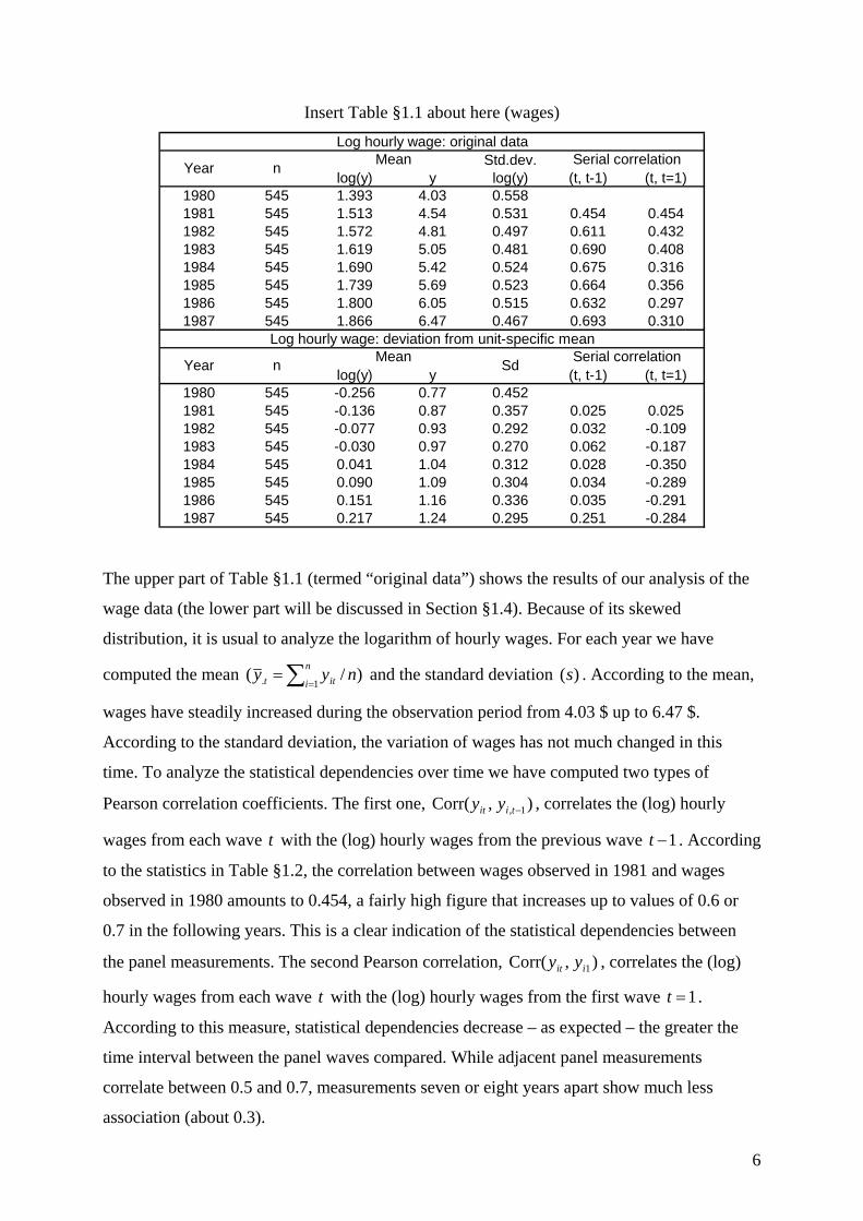
The upper part of Table §1.1 (termed “original data”) shows the results of our analysis of the

wage data (the lower part will be discussed in Section §1.4). Because of its skewed

distribution, it is usual to analyze the logarithm of hourly wages. For each year we have

computed the mean )/(1. ∑=

=n

i itt nyy and the standard deviation )(s . According to the mean,

wages have steadily increased during the observation period from 4.03 $ up to 6.47 $.

According to the standard deviation, the variation of wages has not much changed in this

time. To analyze the statistical dependencies over time we have computed two types of

Pearson correlation coefficients. The first one, ),Corr( 1, −tiit yy , correlates the (log) hourly

wages from each wave t with the (log) hourly wages from the previous wave 1−t . According

to the statistics in Table §1.2, the correlation between wages observed in 1981 and wages

observed in 1980 amounts to 0.454, a fairly high figure that increases up to values of 0.6 or

0.7 in the following years. This is a clear indication of the statistical dependencies between

the panel measurements. The second Pearson correlation, ),Corr( 1iit yy , correlates the (log)

hourly wages from each wave t with the (log) hourly wages from the first wave 1=t .

According to this measure, statistical dependencies decrease – as expected – the greater the

time interval between the panel waves compared. While adjacent panel measurements

correlate between 0.5 and 0.7, measurements seven or eight years apart show much less

association (about 0.3).

7

In the following we will call ),Corr( 1, −tiit yy and ),Corr( 1iit yy serial correlation coefficients

(of order 1 or k ). It has been tempting to call them autocorrelations, but these measures have

a very specific meaning in the context of time series (and panel) analysis.6 The term “serial

correlation”, on the other side, makes clear what is at stake here: ),Corr( 1, −tiit yy and

),Corr( 1iit yy are measures of the temporal (serial) dependencies in the data, which are

apparently quite high in the wage data (though decreasing with temporal distance between

measurements). Later on, we will discuss more concretely possible reasons for these high

serial correlations (Section §1.4).

Insert Table §1.2 about here (union membership)

no member member no member member no member member memberno member 535 76.43 91.96 8.04 91.96 8.04

member 165 23.57 25.45 74.55 25.45 74.55 25.45 74.55 74.55no member 534 76.29 92.88 7.12 91.59 8.41

member 166 23.71 23.49 76.51 27.27 72.73 12.20 87.80 65.45no member 535 76.43 93.08 6.92 90.84 9.16

member 165 23.57 26.67 73.33 33.94 66.06 15.74 84.26 55.15no member 542 77.43

member 158 22.57

1972

1973

n State probability

1970

1971

Year t

Union membership

Survival probability

Conditional transition probability (members)

First-order transition matrix (t, t+1)

Higher-order transition matrix (t=1, t+1)

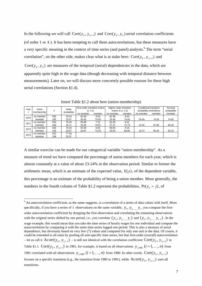
A similar exercise can be made for our categorical variable “union membership”. As a

measure of trend we have computed the percentage of union members for each year, which is

almost constantly at a value of about 23-24% in the observation period. Similar to former the

arithmetic mean, which is an estimate of the expected value, )E(y , of the dependent variable,

this percentage is an estimate of the probability of being a union member. More generally, the

numbers in the fourth column of Table §1.2 represent the probabilities, )Pr( jyit = , of

6 An autocorrelation coefficient, as the name suggests, is a correlation of a series of data values with itself. More specifically, if you have a series of t observations on the same variable, tyyy ,,21, K , you compute the first-order autocorrelation coefficient by dropping the first observation and correlating the remaining observations with the original series shifted by one period, i.e., you correlate ),( ,,32 tyyy K and ),( 1,,21 −tyyy K . In the wage example, this would mean that you take the time series of hourly wages for one individual and compute the autocorrelation by comparing it with the same time series lagged one period. This is also a measure of serial dependence, but obviously based on very few (7) values and computed for only one unit in the data. Of course, it could be extended to all units by pooling all unit-specific time series, but that first-order (overall) autocorrelation – let us call it ),orr(Ac 1, −tiit yy – is still not identical with the correlation coefficient ),Corr( 1, −tiit yy in

Table §1.1. ),Corr( 1, −tiit yy in 1981, for example, is based on all observations ),,1(1981, niyi K= from

1981 correlated with all observations ),,1(1980, niyi K= from 1980. In other words, ),Corr( 1, −tiit yy

focuses on a specific transition (e.g., the transition from 1980 to 1981), while ),orr(Ac 1, −tiit yy uses all transitions.

8

observing the corresponding category j of the dependent variable ity . Within the context of

Markov modeling this is also called a state probability.

To get an idea of the statistical dependencies in the union membership data we compute

conditional percentages: How many of the present union members are still members next

years and how many leave the union? According to the statistics in Table §1.2 nearly three

quarters (25.45%) of the 1970 members quit their union in the following year. Similar

questions can be asked for the non-members: How many enter a union and how many prefer

not to join a union? All in all, the four percentages in each cell of the fifth column of Table

§1.2 constitute a matrix of transition probabilities. Each entry in this matrix estimates a

(conditional) probability, )|Pr( 1, jyky itti ==+ , of being in certain state k of the dependent

variable in the following year, 1, +tiy , given the unit has been in state j of ity in the current

year. This matrix of transition probabilities is the equivalent for the former first-order serial

correlation.7 Its diagonal elements give an indication of the persistence of union membership

and non-membership. According to the statistics in Table §1.2, the probability of remaining in

the same status is quite high (about 75% for members and above 90% for non-members).

We have also computed an equivalent for ),Corr( 1iit yy . These are the higher order transition

probabilities, )|Pr( 1 jyky iit == , in the sixth column of Table §1.2. They condition on

membership status in the first wave )( 1iy . We observe a similar result as in the continuous

case. The longer the time interval between both measurements ity and 1iy , the lower the

diagonal cells in the transition matrix and hence the probability of constant membership

status. For example, while three quarters of the union members are still organized in the

following year, three years later only two thirds (66.06%) abide by their union.

Both examples (wages and union membership) tell the same story. Irrespective of the nature

of our dependent variable, be it continuous or categorical, repeated observations over time 7 Some of you may wonder why in the continuous case one correlates ity (from the present wave) with 1, −tiy

(from the previous wave), while in the categorical case ity (from the present wave) is tabulated with 1, +tiy (from the next wave). This has mainly historical reasons, and is of no practical relevance. For example, we could equally well compute ),Corr( 1, +tiit yy . Traditionally, Markov models have focused on predicting the future (state) distribution of the dependent variable given its present distribution. To this end, we need the state probabilities in the present wave and the transition matrix from the present to the next wave. Regression models for continuous variables, on the other hand, have focused on explaining the present values of the dependent variable with information from the past.

9

will almost always correlate with each other8 and later on we will see why this is the case (see

Section §1.4) and how to cope with it (see Section §1.6). In other words, panel data by no

means include independent information. We have certainly more information than in a cross-

section of n units, but not as much as in a cross-section of TnN ⋅= units. Ignoring these

statistical dependencies is potentially dangerous when applying regression models, because

traditional estimation procedures assume independent observations. Thus, they will estimate

standard errors that tend to be too low, and as a consequence, test statistics will be too high, p-

values correspondingly too low such that significance tests will lead to erroneous conclusions.

Furthermore, although parameter estimates are unbiased, they could be estimated more

efficiently, if the statistical dependencies would be explicitly modeled.

1.3 Describing panel data Before proceeding with a deeper understanding of these statistical dependencies, it is always a

good idea to have a descriptive overview of the data at hand. This is already a difficult task

with cross-section data, but what to do with the much more complex panel data. Simple

techniques are the ones used in the previous section. Means and standard deviations describe

the overall trend and the spread of continuous variables. Proportions do the same job for

categorical data. Correlating a continuous variable (cross-tabulating a categorical variable)

over time informs us about short- and long-term serial dependencies. However, the longer the

time interval between ity and xtiy +, , the more difficult it is to tell the trajectory how the unit

got from ity to xtiy +, . Consider, for example, the transition from 1970 to 1973 in the union

data. According to Table §1.2, forty-nine (9.16%) of the non-members from 1970 were

members of a union in 1973. Not all of them joined a union in 1973. Some may have done so

in preceding years and some may have even joined and again quitted the union in between.

Thus, besides measures of trend, spread, and serial dependence we would like to have more

information on the unit-specific trajectories of the corresponding variables.

8 In all practical situations this correlation will be positive, because above (below) average units tend to remain above (below) the average in the continuous case or to remain in the same state in the categorical case. A negative correlation implies that change is more often observed than stability. A union member will have a high probability of being a non-member next year and again a member in the year to follow, etc. Individuals with high wages this year will have low wages next year and again high wages in the following year, and so on. Such alternating processes are not very realistic.

10

Insert Table §1.3 (sequences) about here

1970 Sequence n % Total0000 442 63.140001 24 3.430010 19 2.710011 7 1.000100 21 3.000101 3 0.430110 4 0.570111 15 2.141000 27 3.861001 3 0.431010 4 0.571011 8 1.141100 8 1.141101 7 1.001110 17 2.431111 91 13.00

no u

nion

mem

ber

unio

n m

embe

r

165

535

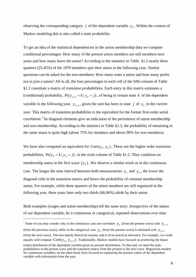
For categorical data it is easy to make tabular summaries because the number of combinations

is limited (at least for short panels). Consider again the union example: If union membership

is coded with a dummy variable (member coded 1, 0 otherwise) a series of zeros and ones

summarizes the membership career of each individual. For example, the series 1000 −−−

indicates that an individual has been out of the union during the observation period except in

the last year 1973. Such a series is also called a sequence. With four measurements over time

and a dichotomous dependent variable there are 1624 = different sequences. Table §1.3

shows the frequency of different sequences of union membership as they appear in the data.

Only two sequences – constant membership )1111( and non-membership )0000( – are

observed more often ( 442=n and 91=n ). The rest of the sample is scattered across the other

sequences and it is, therefore, difficult to detect additional patterns of interest.9 In other

words: While the former measures of trend, spread, and serial dependence may be too coarse,

this technique apparently provides too detailed information (and this information will increase

exponentially with the number of measurements).

It seems to be a much more promising strategy to decompose the heterogeneity of individual

sequences into simpler processes of change. If you go back to the first-order transition

matrices in Table §1.2, a starting hypothesis could be that the pattern of stability and change

that is summarized in these figures is more or less constant in the whole observation period.

This implies the assumption that the differences between single transition matrices are simple

9 $Refer to literature on sequence analysis.

11

random noise and an average of all three matrices describes the process equally well. Finding

the correct transition matrix that describes the observed process is at the heart of Markov

modeling. An even more promising approach is to look at single transitions (e.g., the exit

from a union) and to reconstruct the observed process from this and other transitions.

This is shown in columns 7 and 8 of Table §1.2, which include estimates of conditional

transition probabilities and the probability of surviving for the union members in the first year

1970. A conditional transition probability, )|Pr( 1,1 jyyky tiiit ==== −K , measures the

probability of being observed in category (state) k of the dependent variable, ty , in the

current wave given no change in the former years (i.e., 1iy up to 1, −tiy have the same value,

say, j ). Table §1.2 shows these conditional transition probabilities for the origin state of

union membership )1( =j . For example, of the individuals that are still union members in

1972 more than four fifths (84.26%) leave the union in 1973 and 15.74% remain union

members for another year. Nota bene, these conditional probabilities focus on those

individuals only that have remained union members up to the preceding panel wave and hence

the denominator of the corresponding frequency ratio changes with each panel wave. If you

are interested in seeing what this all means for the original union members from wave 1, you

better look at the probability of survival or the survivor function for short.

)1|1Pr()(S 11 === iit yyt conditions on the union members of 1973 (i.e., 11 =iy ). According

to the statistics in the eighth column of Table §1.2 a little bit more than half (55.15%) of the

original members abide by their union.

12

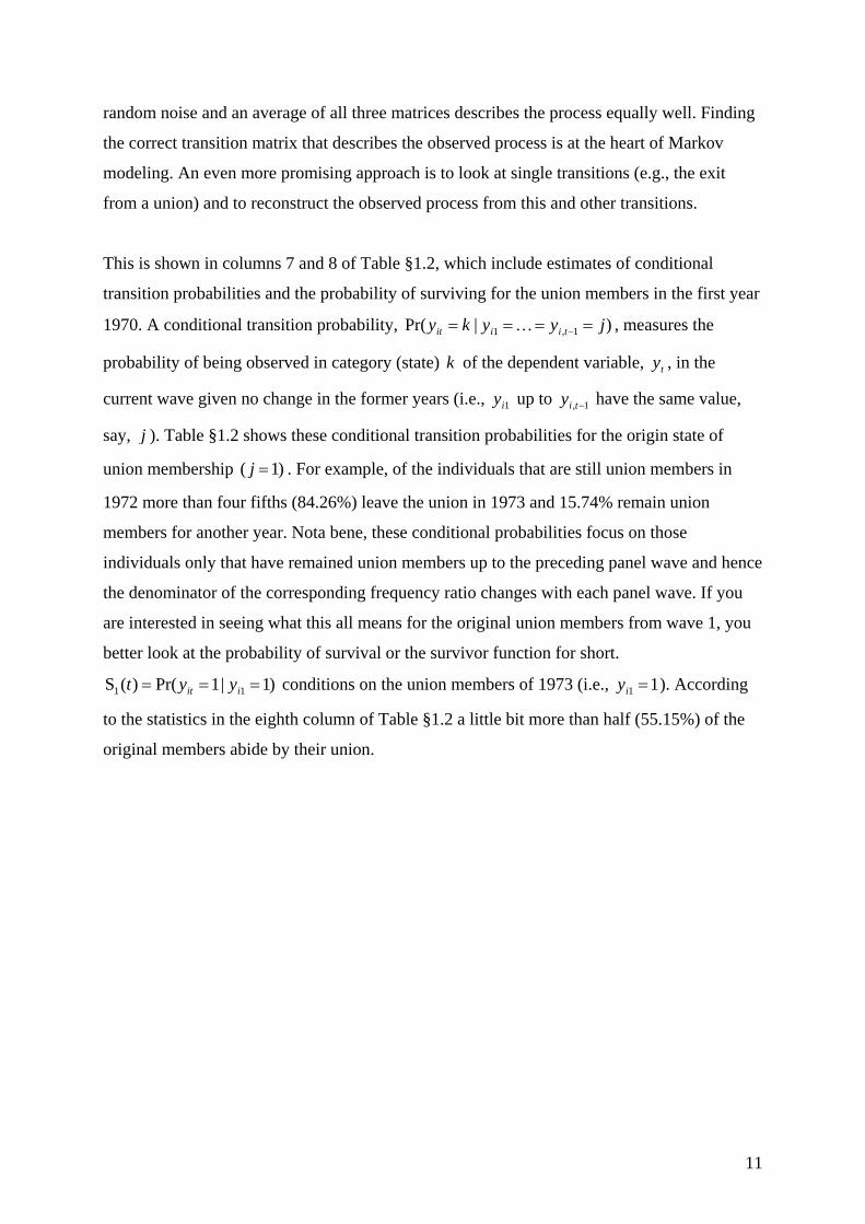
Insert Figure §1.1 (Probability of survival by region) about here (§add perhaps a plot of the

conditional transition probability and survivor for all)

As Figure §1.1 shows, the survivor function is easily plotted in a two-dimensional graph and

by differentiating group-specific survivor functions important information on possible

explanatory factors can be obtained. It appears that union membership is a little less stable in

the Southern states than in the rest of the US, because the probability of surviving declines

faster in the South. We will see later on that the conditional transition probability is the main

variable of interest if one models change in categorical dependent variables. The primary

motivation for the conditioning on the “surviving” units is the observation that patterns of

change may change over time.10

10 Instead of plotting the survivor function, we could have drawn the conditional transition probability. In most cases, however, it will show a much more irregular pattern, because its base – the number of units remaining in the origin state – is declining over time. Thus, the conditional transition probability is based on increasingly smaller number of cases and without a measure of its standard error, it is hard to differentiate random from substantive changes over time.

0.00

0.25

0.50

0.75

1.00

prob

abili

ty o

f sur

viva

l

0 1 2 3 4wave

region = other region = South

13

Insert Table §1.4 (data listing) about here

1981 1982 1983 1984 1985 1986 1987 Mean2.937 3.473 2.971 3.777 4.052 3.293 3.096 3.1742.541 3.086 3.229 2.620 2.691 2.606 2.236 2.6851.972 2.232 2.554 2.905 2.966 2.990 3.132 2.6252.338 2.416 2.514 2.648 2.636 2.719 2.769 2.5502.510 2.593 2.564 2.465 2.613 2.645 2.282 2.5302.391 2.356 2.562 2.636 2.643 2.807 2.813 2.5232.412 2.315 2.508 2.599 2.700 2.741 2.663 2.5181.962 2.276 2.195 2.428 2.723 2.966 3.065 2.4541.574 1.442 2.547 2.991 3.011 3.099 3.097 2.4372.531 2.171 2.197 2.455 2.069 2.429 2.602 2.377⋅⋅⋅ ⋅⋅⋅ ⋅⋅⋅ ⋅⋅⋅ ⋅⋅⋅ ⋅⋅⋅ ⋅⋅⋅ ⋅⋅⋅

0.030 0.688 0.676 0.647 0.955 1.564 1.301 0.7930.898 0.970 0.804 1.306 1.477 -0.981 0.791 0.7820.541 0.195 0.383 1.104 1.066 1.202 1.046 0.7770.289 0.906 0.339 1.213 1.502 1.277 -0.191 0.7641.079 0.840 1.508 1.021 0.543 0.115 0.313 0.7630.075 0.172 0.948 1.227 0.435 0.639 1.678 0.7600.606 0.865 0.512 0.684 1.000 1.435 1.177 0.738-1.417 -0.670 0.703 0.713 0.820 1.069 1.039 0.414-0.149 0.181 -0.036 0.397 0.973 0.563 0.759 0.333

For continuous data it is even more difficult to get an overview of the unit-specific

trajectories. In most cases tabular presentations are more or less data listings without any kind

of data summary, because continuous variables can take on so many different values. Table

§1.4 demonstrates that without classifying wages into different classes each income trajectory

is more or less unique. In principal, graphical displays are a better way of presenting this

differentiated information, but if the sample size gets large these techniques usually fail

because of heavy overprinting. Therefore, the left panel of Figure §1.2 uses only a subsample

of the original wage data to provide a graphical impression of individual differences in level

and change. We have selected ten individuals with the highest and another ten with the lowest

average wages.11 You can easily imagine how this line plot would look like, if we had used

the data of all 545=n individuals. Possibly, we would have only hatched the plot region.12

11 Actually, we plotted only nine of the low wage trajectories, because one individual had extremely low wages. 12 In principle, such line plots could also be used for categorical data. But here we are faced with the opposite problem. The dependent variable includes only few distinct values resulting in lots of lines plotted on top of each other.

14

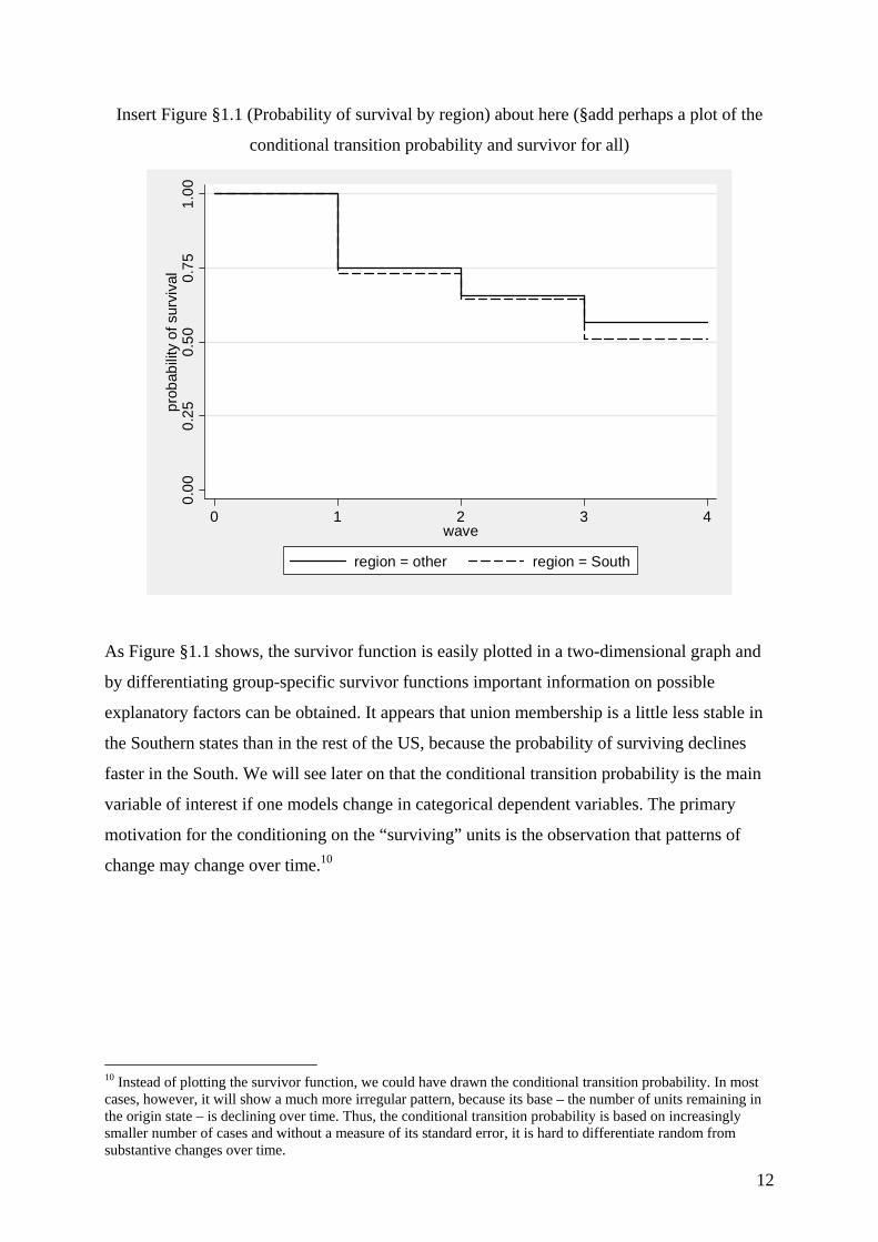
Insert Figure §1.2 (income trajectories: very high and very low wages) about here.

Nevertheless, Figure §1.2 provides some interesting insights into panel data in general and the

wage data in particular. Imagine first two different groups behind these ten respectively nine

income trajectories. The two thick black lines illustrate the linear wage growth observed in

both groups. Obviously, the first group – on average – earns much higher wages than the

second group and it seems as if their wages grow a little bit faster during the course of the

panel (although the latter is hardly visible; both lines are more or less in parallel). Thus, if the

sample size is not too large and if the data are as clearly structured as the ones in Figure §1.2,

line plots provide important information on possible explanatory factors (similar to survivor

plots in the categorical case).

Now image we had estimated a linear growth model for each individual. This is shown in the

right panel of Figure §1.2. Similar to the two (thick black) group-specific lines these unit-

specific lines differ with respect to level and amount of growth. In principle, each unit has its

own intercept and slope. At the moment, this plot simply illustrates the internal heterogeneity

within each group. Later on we will have to ask how to model this unit-specific variance of

slopes and intercepts.

-20

24

log

hour

ly w

age

1980 1982 1984 1986 1988Year

-20

24

log

hour

ly w

age

1980 1982 1984 1986 1988Year

15

Finally, Figure §1.2 shows that the overall variation of the wages derives from two sources:

one is the heterogeneity of average wages between individuals (between-unit variance), the

other is the heterogeneity of yearly wages over time for each individual (within-unit

variance). Let ∑ ∑= =⋅=

n

i

T

t it Tnyy1 1.. )/( be the overall arithmetic mean of all yearly wages for

all individuals and Tyy T

i iti /1. ∑=

= the corresponding mean for all yearly wages of one

specific individual i . With this notation estimates of both variance terms can be computed as

follows:

)1(

)(ˆ)Var(

1

)(ˆ)Var(

1 1

2.

2

1

2...

2

−⋅

−==

−

−==

∑∑

∑

= =

=

Tn

yyWithin

n

yyBetween

n

i

T

tiit

e

n

ii

u

σ

σ. (§1.1)

For the total sample of all 545=n individuals we estimate 0.3907 ˆ 2 =uσ and 0.3872ˆ 2 =eσ ,

indicating that in this sample the variance between units is nearly as large as the variance

within units. In other words, wage heterogeneity across different individuals does not differ

very much from wage heterogeneity across different years (taking into account the average

level of wages for each individual). Furthermore, both variance estimates can be used to

compute an overall measure of serial dependence, which is known as the intra-class

correlation coefficient ICCρ :

22

2

eu

uICC σσ

σρ+

= . (§1.2)

Formally, it is the amount of between-unit variance as a proportion of the total variance of the

dependent variable. Given certain assumptions about the underlying process, it can be shown

that it measures the correlation between any two measurements within the unit-specific (thus

“intra-class”) time series.13 Originally, the intra-class correlation coefficient has been used as

a measure of test-retest reliability (a test-retest study is equivalent to a two wave panel study).

In our case it measures the “closeness” of measurements on the same unit relative to the

13 We will discuss these assumptions in greater detail in Chapter §, but you should note that there are different versions of the intra-class correlation coefficient and equation (§1.3) presents a very specific one.

16

closeness of measurements between different units. For the wage data it amounts to

.50450ˆ =ICCρ , indicating again a fairly high amount of serial dependence.14

1.4 Explaining panel data Having an idea of how our dependent variable looks like, we now turn to the question of how

to explain its distribution over time and between units. Why do some individuals earn higher

wages or have higher probabilities of union membership? Why do wages increase more

steeply for some individuals? Why is union membership rather stable for some individuals,

but a more transient phenomenon for others? These questions concern the level and the

change of the dependent variable. In the following our primary interest is not in substantive

arguments concerning the two examples (which would imply an excursus, e.g., into human

capital theory or rational choice models of political action). Instead we will provide a synopsis

of the typical explanatory variables that are used to answer these kinds of questions and

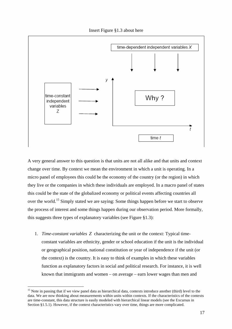
discuss their statistical properties. This is illustrated in Figure §1.3 with an empty line plot, in

which you can imagine the time trajectories of your dependent variable (wages, union

membership or whatever you like). The question is now: Why do they behave the way they

do?

14 You may wonder why the intra-class correlation coefficient is much smaller than the first-order serial correlations of Table §1.1. You should note, however, that both statistics are based on different concepts: While

ICCρ is a measure of absolute agreement, the correlations of Table §1.1 are measures of relative agreement (Rabe-Hesketh & Skrondal, 2005: 14).

17

Insert Figure §1.3 about here

A very general answer to this question is that units are not all alike and that units and context

change over time. By context we mean the environment in which a unit is operating. In a

micro panel of employees this could be the economy of the country (or the region) in which

they live or the companies in which these individuals are employed. In a macro panel of states

this could be the state of the globalized economy or political events affecting countries all

over the world.15 Simply stated we are saying: Some things happen before we start to observe

the process of interest and some things happen during our observation period. More formally,

this suggests three types of explanatory variables (see Figure §1.3):

1. Time-constant variables Z characterizing the unit or the context: Typical time-

constant variables are ethnicity, gender or school education if the unit is the individual

or geographical position, national constitution or year of independence if the unit (or

the context) is the country. It is easy to think of examples in which these variables

function as explanatory factors in social and political research. For instance, it is well

known that immigrants and women – on average – earn lower wages than men and

15 Note in passing that if we view panel data as hierarchical data, contexts introduce another (third) level to the data. We are now thinking about measurements within units within contexts. If the characteristics of the contexts are time-constant, this data structure is easily modeled with hierarchical linear models (see the Excursus in Section §1.5.1). However, if the context characteristics vary over time, things are more complicated.

18

native born employees. Much research has also been done on the effect of regime type

(democracy versus dictatorship) on economic growth or on the effect of geographical

position on foreign trade.

2. Time-dependent variables X characterizing the unit or the context: Examples include

variables like labor force experience, on-the-job training, economic growth (of the

economy or the firm), amount of public spending, etc. Again, it is quite obvious that

these variables can be used as explanatory factors in different settings. For example,

human capital theorists assume that wages increase with labor force experience and

on-the-job training. Organization researchers may add that pay rises are much easier in

prospering companies. Or consider a panel analysis of countries: Here we could

expect, e.g., that economic growth increases government stability.

3. Time t : Finally, many researchers also mention “time” as an explanatory variable.

However, it is questionable whether time itself is an explanatory variable of its own. In

many cases, time is only an indicator for other characteristics that change over time

(e.g., labor force experience or economic growth). Sometimes, however, we have no

idea of what these time-dependent characteristics might be or we lack the necessary

data to control for them. In these cases it is a good idea to control for possible time

trends in the data by including a variable “time” into the statistical model (see below).

Depending on your research interests it is also advisable to think about a good

definition of time. It could be chronological time (e.g., as an indicator of the business

cycle) or time since an event (e.g., entry into the labor force as an indicator of labor

force experience). It is even possible to include different time variables into the model

(e.g., chronological time and labor force experience) as long as these time variables

are not linearly dependent.16

A necessary condition for all kinds of explanatory variables is that they show some variation.

Put differently, constants are useless when it comes to explaining variation in the dependent

variable. Technically, time-dependent variables X vary across units and measurements, time-

constant variables Z vary only across units, and time t varies only across measurements.

There may be a problem with time-constant variables describing the context, because usually

we have fewer contexts than units (in the extreme case one context for all units, e.g., a sample

16 The classical example comes from cohort analysis, which tries to disentangle the effects of generation, maturation and time period. If, for example, in an analysis of political attitudes someone tries to include year of birth (generation), age in years (maturation) and year of the interview (time period) as independent variables, such a model will not be feasible because all three time variables are linearly dependent: (year of interview) = (year of birth) + age. However, with longitudinal data )2( ≥T it is possible to include two of these variables into the model (e.g., year of birth and age).

19

of individuals from one country). Thus, if a context variable is time-constant, there should

exist at least several contexts in the data to observe some variation. Time-dependent variables

characterizing the context usually pose no problems. In the extreme case (only one context),

there is at least some variation over time (but not over units).

There is one possible misunderstanding with Figure §1.3: The text and the figure (especially

the horizontal arrows) may suggest that Z only affects the level of the dependent level

)( YZ → , while X only affects the change of Y )( YX Δ→Δ . This is not the case and the

following section will discuss possible relationships between X , Z , and Y more thoroughly.

The horizontal arrows should simply indicate that Z remains constant over time, while the

vertical arrows should indicate that X can change from one time point to the next. Note also

that not many explanatory variables are time-constant by nature. Remember the two

aforementioned examples “school education” and “national constitution”. Both may very well

change (by further education or by political reforms), but after labor market entry it may be

acceptable to treat school (!) education as time-constant and constitutional change may be so

seldom within one country that the national constitution may be treated as a stable

characteristic. Very often we also lack the necessary temporal information, which forces us to

treat a time-dependent variable as if it were time-constant.

Having discussed possible explanatory factors for our dependent variable, we can now come

back to the question why measurements over time show high degrees of serial correlation.

The answer is now quite obvious: First of all, having certain characteristics Z that do not

change over time causes the dependent variable to have similar values next period. An Afro-

American individual having a low income this year will not have a very much different

income next year (all other factors held constant).17 A second source of serial dependence are

the time-dependent variables X . This may be a bit surprising, because we have just argued

that the fact that these variables change over time explains why our dependent variable

changes as well (and is not the same next year). However, this does not mean that the time-

dependent characteristics change every year and/or to a large amount. Although they may not

be identical next year, they may nevertheless correlate over time (in a similar way as the

dependent variable does). This serial correlation among the time-dependent variables X is

17 The situation resembles very much the spurious causal correlation problem known from the analysis of cross-sectional data. Two variables x and y may be correlated because both of them are associated with a third

variable z . With panel data, measurements itii yyy ,,2,1 K will be correlated because all of them are correlated with a “third” variable z that characterizes the unit.

20

another source of statistical dependence among the measurements of the dependent variable.

Finally, that a given unit has a certain value of the dependent variable this year may have a

direct impact on the dependent variable’s value next year. Consider, e.g., the case of union

membership: Being member of a union implies having contact with other people of similar

opinions and being exposed to political ideas of the organization, which may increase positive

sentiments about the union movement and thus increase membership stability.

With these arguments in mind, it becomes obvious why measurements of the dependent

variable over time must correlate. While the first two arguments are purely statistical (often

termed spurious state dependence), the later one provides a substantive cause of serial

correlation (often termed true state dependence). To the extent that we are able to control for

all relevant time-constant and time-dependent explanatory variables ( Z , X and lagged

values of Y if necessary), measurements of the dependent variable should be independent

over time. Or more specifically, the residuals of this model should be pure random noise.

This can be shown with the data in the lower part of Table §1.1. Having made the distinction

between time-constant and time-dependent explanatory variables (including time itself), we

realize that the serial correlations computed earlier have two components: one is due to the

time-constant cross-sectional variation (some individuals – on average – have higher incomes

than other individuals) and the other is due to variation in the time dimension. The time-

constant cross-sectional variation is easily controlled away by subtracting from each data

value ity the unit-specific mean Tyy T

i iti /1. ∑=

= . Let us call the transformation )( .iit yy −

“demeaning”. The lower part of Table §1.1 shows the first-order serial correlations computed

on the demeaned data, which are all much smaller than those computed on the original data.

As a final point in this section let us contemplate why serial correlations get smaller with

increasing time lag between measurements. The answer is quite easy. Let us begin with an

extreme case: If only time-constant explanatory variables Z determine the process and if they

only affect the level of the dependent variable (effects being constant over time), the

dependent variable will have the same values in each panel wave and nothing changes at all

(resulting in serial correlations that are all equal to 1). This is a very unrealistic case and in

fact we do not need panel data to analyze it (the first cross-section will suffice). However, if

the effects of the time-constant explanatory variables change over time, if Z also affects the

change of Y )( YZ Δ→ , if time-dependent explanatory variables X come into play and if

21

random error exists, the values of Y are not the same next year and possibly these “noise

factors” will accumulate over time. All of this results in decreasing higher order serial

correlations as they are shown in the upper part of Table §1.1.

1.5 Modeling panel data In this section we discuss how the independent variables may influence the dependent

variable and how we can formalize this. When we say “formalize”, we mean a mathematical

model (a regression function) that tells us numerically how the values of the dependent

variable are related to the values of the independent variables. As already mentioned, we can

model either the level )(Y or the change )( YΔ of the dependent variable and we can use

either the level ),( ZX or the change )( XΔ of our independent variables as explanatory

factors ( 0=ΔZ by definition). A few examples from our two data sets and other sources shall

illustrate this:

a) ),( YZX → : For example, human capital theory asserts that higher levels of labor force

experience are associated with higher earned incomes suggesting a (positive) association

between the level of income )(Y and a time-dependent variable measuring employment

duration )(X . Rational choice models assume that the benefits of union membership are

higher for low-status employees suggesting a (negative) association between the level of

school education ( Z , assumed to be time-constant after labor market entry) and the level

of union membership )(Y . As you may have noticed, these are also the kinds of

relationships we normally use in the analysis of cross-sectional data, but obviously they

can also be applied to panel data. Nevertheless, this observation raises the question why

we should use these more complicated and possibly more costly data to answer simple

cross-sectional questions. As we shall see later on (Section §1.6), panel data provides

additional information that allows us to avoid some of the specification errors that are

typical for cross-sectional data.

b) )( YX →Δ : Besides models of type (a), we sometimes have applications where the level

of the dependent variable is the result of changes in the independent variables. A good

example is adaptive behavior. For example, subjective well-being )(Y is much less related

to absolute income )(X than to income changes )( XΔ . This can be illustrated with

research on the effects of unemployment. Becoming unemployed and having less income

is usually associated with significantly less subjective well-being. In the long run,

however, people often return to their former levels of subjective well-being, because they

adapt to the new financial situation.

22

c) ),( YZX Δ→ : This type of relationship is typical for many change processes in the

natural sciences. For example, radioactive decay )( YΔ is assumed to be related to the

(time-dependent) quantity of radioactive nuclei )(X that has not yet decayed. In our

income data, the rate of income increases )( YΔ could be related to (time-constant)

ethnicity )(Z , because discrimination theories suggest that ethnic minorities are less often

promoted than members of the majority population. Another example is the higher life

expectancy of women compared to men. In this case, the change of physical existence

( YΔ , death) is related to the time-constant variable gender )(Z .

d) )( YX Δ→Δ : When we think about processes of change, this kind of relationship always

comes to our mind. The dependent variable changes, because something changes for the

unit or the context (cf. the discussion in the former section). Thus, it is not necessary to

provide any specific examples. But you should note the connections with relationships of

the first type ),( YZX → . For example, if we interpret regression coefficients )(β from

cross-sectional models we say that a unit change of the independent variable causes a

change of β units in the dependent variable. Thus, if models of type (a) are true, models

of type (d) are true as well. Later on, we will see more formally that it is easy to transform

models of type (a) into models of type (d). In other words, they are conceptually

equivalent. Nevertheless, it is important to make a distinction between them, because

estimates based on data in levels generally will not be identical to estimates based on

changes, although both models are conceptually equivalent. Besides that, we can think of

examples where models of type (d) are true, while models of type (a) are not. These are

processes, where the initial levels of X and Y are independent, but changes in X cause

changes in Y (Menard 2002: pp. 55).

e) )( txt YY →− : Finally, as already noted in the previous section, there are instances of true

state dependence, in which previous levels influence the present level of the dependent

variable. Models including these kinds of relationships are called dynamic, because they

describe the development of the dependent variable given its previous history. Consider,

for example, government spending: The federal government’s budget is fixed in large

parts by decisions that have been made years before. Thus, only a minor portion of the

budget is available for new policies and large parts of present government spending can be

explained by last year’s budget. Or remember the union example in the last section: Being

member of a union may increase positive sentiments about the union movement and thus

increase membership stability. Models of partial adjustment and adaptive expectations

23

($references) that have been popularized in economics also result in relationships, in

which previous levels influence the present level of the dependent variable.

In the following, we discuss models for levels (§1.5.1 and §1.5.2) and change (§1.5.3 and

§1.5.4) of the dependent variable focusing on relationships of type (a) and (d). We conclude

with a short view on the other types of relationships, including models with lagged variables

and dynamic models (§1.5.5). Throughout we will make a distinction between continuous and

categorical variables. As already mentioned, models for continuous variables focus on the

expected value, )E(y , of the dependent variable, while models for categorical variables focus

on the probability, )Pr( kyit = , of observing a certain category, say k , of the dependent

variable.

1.5.1 Modeling the level of continuous dependent variables For continuous dependent variables, a typical panel regression model in levels is a simple

extension of the well-known linear regression model for cross-section data. The following

linear model regresses the expected value of a continuous and time-dependent dependent

variable Y on a set of independent variables, which – according to the discussion in the

previous section – may be either time-constant )(Z or time-dependent )(X . By using

appropriate subscripts, we take care of the time dimension in the data:

444 3444 21K

4444 34444 21K

partconstant -time

11

partdependent -time

110 )()E( jijikitkitit zzxxty γγβββ ++++++= . (§1.3)

Subscript i refers to the ni ,,1K= units, which have been observed at Tt ,,1K= equidistant

points in time. ity denotes the value of the dependent variable for individual i at time point t .

It is modeled as a linear function of the values of j time-constant ),,( 1 jii zz K and k time-

dependent independent variables ),,( 1 kitit xx K .18 kββ ,,1 K and jγγ ,,1 K denote the

corresponding regression coefficients. The regression constant )(0 tβ determines the overall

level of the dependent variable. Since its level may change over time, the regression constant

can be any function of time, if it is necessary to control for time trends (or 00 )( αβ =t , if it is

not). Possible functions of time include linear ))(( 100 tt ααβ += , quadratic

18 Readers familiar with the linear regression model might miss an error term in equation (§1.3). They should remember, however, that at this point of our discussion we only look at the expected value of the dependent variable and thus, the systematic part of the regression model. Nevertheless, it will be necessary to consider an error term when we discuss the estimation of (§1.3) (see Section §1.6).

24

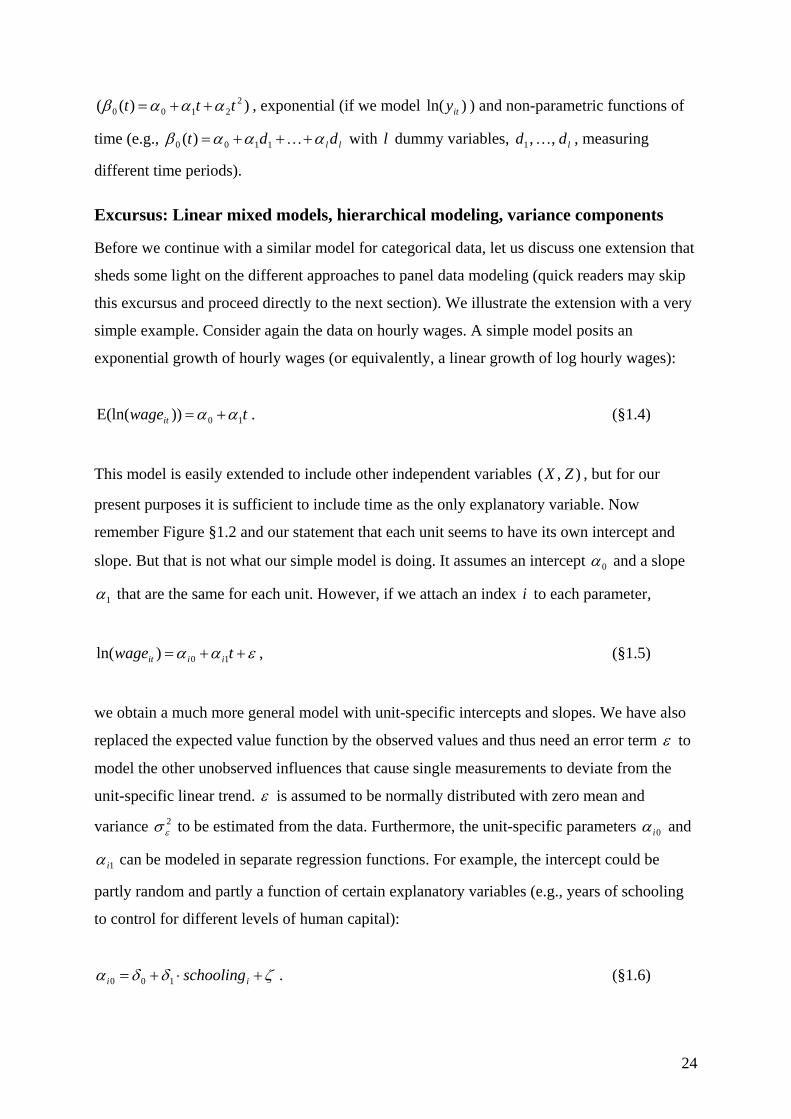
))(( 22100 ttt αααβ ++= , exponential (if we model )ln( ity ) and non-parametric functions of

time (e.g., ll ddt αααβ +++= K1100 )( with l dummy variables, ldd ,,1 K , measuring

different time periods).

Excursus: Linear mixed models, hierarchical modeling, variance components

Before we continue with a similar model for categorical data, let us discuss one extension that

sheds some light on the different approaches to panel data modeling (quick readers may skip

this excursus and proceed directly to the next section). We illustrate the extension with a very

simple example. Consider again the data on hourly wages. A simple model posits an

exponential growth of hourly wages (or equivalently, a linear growth of log hourly wages):

twageit 10))E(ln( αα += . (§1.4)

This model is easily extended to include other independent variables ),( ZX , but for our

present purposes it is sufficient to include time as the only explanatory variable. Now

remember Figure §1.2 and our statement that each unit seems to have its own intercept and

slope. But that is not what our simple model is doing. It assumes an intercept 0α and a slope

1α that are the same for each unit. However, if we attach an index i to each parameter,

εαα ++= twage iiit 10)ln( , (§1.5)

we obtain a much more general model with unit-specific intercepts and slopes. We have also

replaced the expected value function by the observed values and thus need an error term ε to

model the other unobserved influences that cause single measurements to deviate from the

unit-specific linear trend. ε is assumed to be normally distributed with zero mean and

variance 2εσ to be estimated from the data. Furthermore, the unit-specific parameters 0iα and

1iα can be modeled in separate regression functions. For example, the intercept could be

partly random and partly a function of certain explanatory variables (e.g., years of schooling

to control for different levels of human capital):

ζδδα +⋅+= ii schooling100 . (§1.6)

25

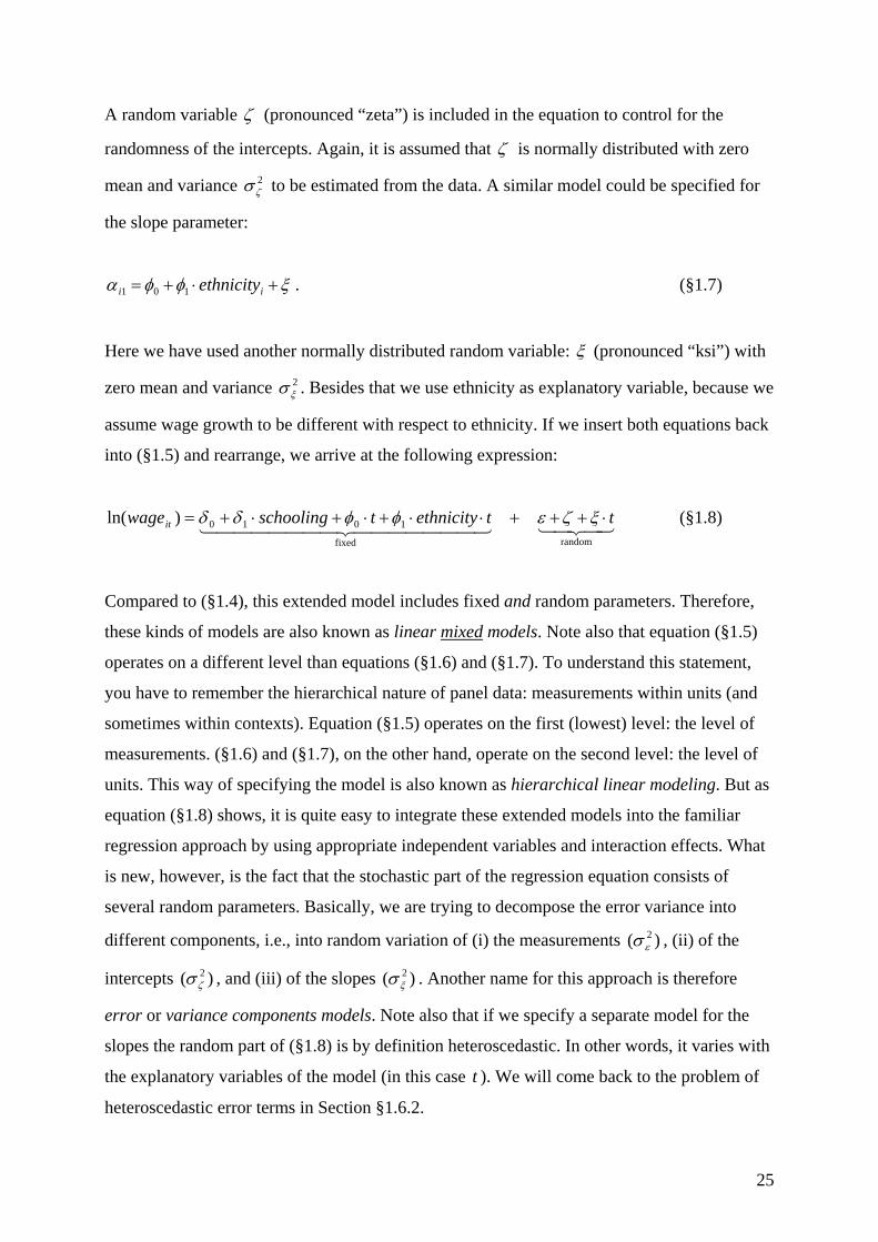
A random variable ζ (pronounced “zeta”) is included in the equation to control for the

randomness of the intercepts. Again, it is assumed that ζ is normally distributed with zero

mean and variance 2ζσ to be estimated from the data. A similar model could be specified for

the slope parameter:

ξφφα +⋅+= ii ethnicity101 . (§1.7)

Here we have used another normally distributed random variable: ξ (pronounced “ksi”) with

zero mean and variance 2ξσ . Besides that we use ethnicity as explanatory variable, because we

assume wage growth to be different with respect to ethnicity. If we insert both equations back

into (§1.5) and rearrange, we arrive at the following expression:

434214444444 34444444 21randomfixed

1010)ln( ttethnicitytschoolingwageit ⋅+++⋅⋅+⋅+⋅+= ξζεφφδδ (§1.8)

Compared to (§1.4), this extended model includes fixed and random parameters. Therefore,

these kinds of models are also known as linear mixed models. Note also that equation (§1.5)

operates on a different level than equations (§1.6) and (§1.7). To understand this statement,

you have to remember the hierarchical nature of panel data: measurements within units (and

sometimes within contexts). Equation (§1.5) operates on the first (lowest) level: the level of

measurements. (§1.6) and (§1.7), on the other hand, operate on the second level: the level of

units. This way of specifying the model is also known as hierarchical linear modeling. But as

equation (§1.8) shows, it is quite easy to integrate these extended models into the familiar

regression approach by using appropriate independent variables and interaction effects. What

is new, however, is the fact that the stochastic part of the regression equation consists of

several random parameters. Basically, we are trying to decompose the error variance into

different components, i.e., into random variation of (i) the measurements )( 2εσ , (ii) of the

intercepts )( 2ζσ , and (iii) of the slopes )( 2

ξσ . Another name for this approach is therefore

error or variance components models. Note also that if we specify a separate model for the

slopes the random part of (§1.8) is by definition heteroscedastic. In other words, it varies with

the explanatory variables of the model (in this case t ). We will come back to the problem of

heteroscedastic error terms in Section §1.6.2.

26

1.5.2 Modeling the level of categorical dependent variables The approach in Section 1.5.1 is easily transferred to categorical dependent variables, so that

we can be rather brief. If k denotes the category of Y we are interested in (e.g., being

member of a union), then the probability, )Pr( kyit = , of observing category k for unit i at

time point t equals the following expression:

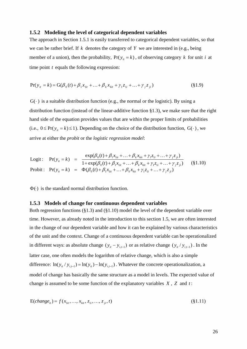
))(G()Pr( 11110 jijikitkitit zzxxtky γγβββ ++++++== KK (§1.9)

)G( ⋅ is a suitable distribution function (e.g., the normal or the logistic). By using a

distribution function (instead of the linear-additive function §1.3), we make sure that the right

hand side of the equation provides values that are within the proper limits of probabilities

(i.e., 1)Pr(0 ≤=≤ kyit ). Depending on the choice of the distribution function, )G( ⋅ , we

arrive at either the probit or the logistic regression model:

))(()Pr(:Probit))(exp(1

))(exp()Pr(:Logit

11110

11110

11110

jijikitkitit

jijikitkit

jijikitkitit

zzxxtkyzzxxt

zzxxtky

γγβββγγβββ

γγβββ

++++++Φ==+++++++

++++++==

KK

KK

KK

(§1.10)

)(⋅Φ is the standard normal distribution function.

1.5.3 Models of change for continuous dependent variables Both regression functions (§1.3) and (§1.10) model the level of the dependent variable over

time. However, as already noted in the introduction to this section 1.5, we are often interested

in the change of our dependent variable and how it can be explained by various characteristics

of the unit and the context. Change of a continuous dependent variable can be operationalized

in different ways: as absolute change )( 1, −− tiit yy or as relative change )/( 1, −tiit yy . In the

latter case, one often models the logarithm of relative change, which is also a simple

difference: )ln()ln()/ln( 1,1, −− −= tiittiit yyyy . Whatever the concrete operationalization, a

model of change has basically the same structure as a model in levels. The expected value of

change is assumed to be some function of the explanatory variables X , Z and t :

),,,,,,()E( 11 tzzxxfchange jiikititit KK= (§1.11)

27

On the right hand side, we have included only the absolute level of the explanatory variables

X and Z , but as we see later on (Section 1.5.5) this could include change and lagged

variables as well.

Now consider again the model in levels (§1.3). For two arbitrary time points, t and 1−t , it

looks as follows:

jijitkiktiti

jijikitkitit

zzxxtytzzxxtyt

γγβββγγβββ

++++++−=−++++++=

−−− KK

KK

111,1,1101,

11110

)1()E(:1)()E(:

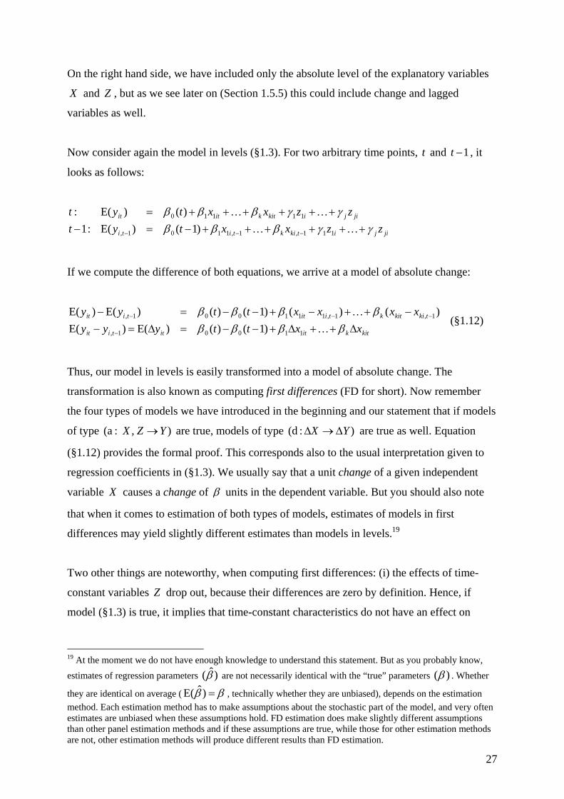
If we compute the difference of both equations, we arrive at a model of absolute change:

kitkitittiit

tkikitktiittiit

xxttyyyxxxxttyy

Δ++Δ+−−=Δ=−−++−+−−=−

−

−−−

ββββββββ

K

K

11001,

1,1,111001,

)1()()E()E()()()1()()E()E( (§1.12)

Thus, our model in levels is easily transformed into a model of absolute change. The

transformation is also known as computing first differences (FD for short). Now remember

the four types of models we have introduced in the beginning and our statement that if models

of type ), :(a YZX → are true, models of type ):(d YX Δ→Δ are true as well. Equation

(§1.12) provides the formal proof. This corresponds also to the usual interpretation given to

regression coefficients in (§1.3). We usually say that a unit change of a given independent

variable X causes a change of β units in the dependent variable. But you should also note

that when it comes to estimation of both types of models, estimates of models in first

differences may yield slightly different estimates than models in levels.19

Two other things are noteworthy, when computing first differences: (i) the effects of time-

constant variables Z drop out, because their differences are zero by definition. Hence, if

model (§1.3) is true, it implies that time-constant characteristics do not have an effect on

19 At the moment we do not have enough knowledge to understand this statement. But as you probably know, estimates of regression parameters )ˆ(β are not necessarily identical with the “true” parameters )(β . Whether

they are identical on average ( ββ =)ˆE( , technically whether they are unbiased), depends on the estimation method. Each estimation method has to make assumptions about the stochastic part of the model, and very often estimates are unbiased when these assumptions hold. FD estimation does make slightly different assumptions than other panel estimation methods and if these assumptions are true, while those for other estimation methods are not, other estimation methods will produce different results than FD estimation.

28

change of the dependent variable. (ii) If one assumes the time trend to be linear, i.e.

tt 100 )( ααβ += , it will be eliminated as well because 11010 ))1(()( ααααα =−+−+ tt .

After seeing the first result (i), you might ask: How is it possible to specify models in which

the level of a time-constant independent variable explains the change in Y ? In other words,

how are models of type (c) ),( YZX Δ→ feasible? Well, consider the former equation (§1.8)

that assumes wage growth to be different for different ethnicities. To make things simple, we

switch back to the expected value of Y and use a simple dummy variable for ethnicity

(ethnicity=1: Afro-American, ethnicity=0: other). If we compute first differences of (§1.8),

we arrive at the following model of change:

iit ethnicitywage ⋅+=Δ 10))ln(E( φφ .

As expected, schooling, which is also assumed to be time-constant, cancels out. But the other

time-constant variable “ethnicity” is still part of the model. More generally speaking, any time

we interact a time-constant with a time-dependent variable in the model on levels of Y , this

time-constant variable is also part of a model on the change of Y . In our simple model of

change, both parameters have an interesting interpretation. 0̂φ estimates the overall linear

trend of log hourly wages and 1̂φ estimates how much this trend is different for Afro-

American employees.

1.5.4 Models of change for categorical dependent variables Models of change for categorical variables are less obvious. There are different options

discussed in the literature. One of them uses the previous value of Y )( 1, −tiy as an

independent variable in a model of levels like (§1.9). Thus, effects of X , Z and t are

estimated controlling for the former status of the unit. Methods for these kinds of dynamic

models, however, are not readily available for categorical data. Another option that originates

from the analysis of tabular data is Markov modeling. In this case one tries to find a simple

structure for the various transition matrices observed over time (cf. Table §1.2). One approach

that fits perfectly in our line of thinking picks out one category of the dependent variable and

models its change. More specifically, it models the conditional transition probability of

making a change from category j to category k of the dependent variable, given the unit has

been observed in category j in all former measurements:

29

))(G()|Pr( 111101,1 jijikitkittiiit zzxxtjyyky γγβββ ++++++===== − KKK (§1.13)

Again, )G(⋅ is a suitable distribution function to make sure that the right hand side of the

equation provides values that are within the proper limits of probabilities (i.e.,

1)|Pr(0 1,1 ≤====≤ − jyyky tiiit K ). As will discussed in Chapter §, )G(⋅ is either the

logistic or the extreme value distribution.

The opposite of a change from j to k is stability or “survival” in the former state j (see the

survivor function in Figure §1.1). Therefore, these kinds of methods are termed survival

analysis. The (sudden) change from j to k is also called an event and some people prefer the

term event history analysis. As equation (§1.13) shows one usually prefers to model change

and not the opposite (survival). For descriptive purposes the survivor function is perfect (and

sometimes easier to analyze than the conditional transition probability, cf. footnote §10). But

for explanatory purposes one uses the conditional transition probability, because it measures

the current rate of change for those who are still at risk, while the survival probability

incorporates the history of all previous transitions and non-transitions. Thus, the conditional

transition probability is a recent measure of change, which you need when you assume that

the process itself changes over time (e.g., when you assume that the probability of union

membership increases with membership duration). Moreover, it can be shown that the

conditional transition probability is a more fundamental parameter of the process from which

all the parameters (survival probability, unconditional transition probabilities, etc.) derive.

1.5.5 Additional models In the preceding sections we have discussed models for levels and change of the dependent

variable mostly focusing on relationships of type ),:a( YZX → and ):d( YX Δ→Δ . But as

we have already seen in one example of Section §1.5.3, other types of relationship between

independent and dependent variables are equally possible (including YX Δ→ , YX →Δ , and

any combination thereof). In the following chapters we will focus on functional forms like

(§1.3), (§1.9), (§1.11), and (§1.13). All of them are called static models, because the current

level (or change) of Y is a function of current levels (or change) of the independent variables.

For this introductory textbook, this is perfectly alright, but you should know that even more

complicated specifications are possible. The right hand side may include past values of the

30

time-dependent explanatory variables (e.g., K,, 2,11,1 −− titi xx ). This would be called a

distributed lag model, because the explanatory variables affect the dependent variable with a

time lag. Furthermore, a so called dynamic model results if the right hand side includes lagged

values, K,, 2,11,1 −− titi yy , of the dependent variable. Finally, all the models posit that there is no

feedback between X and Y , which may be an unrealistic assumption in some applications.

Consider, for example, the relation between union membership and wages. Some economists

ask whether there is a wage premium for union members. On the other hand, it is not

unrealistic to assume that some employees become union members because they expect

higher wages from being a union member. These kinds of reciprocal relationships )( YX ↔

are called (somewhat irritating) non-recursive models, while the former unidirectional

relationships are termed recursive. Non-recursive and dynamic models are extremely difficult

to handle and will not be covered in this book.

1.6 Estimating models for panel data Having discussed how we can put our hypotheses into a formal model, we now turn to the

question of how to find “good” estimates of the model parameters. When estimating the

model with empirical data, our first goal is to reveal the “true” parameters that were “really”

operating when the values of the dependent variable have been observed. The problem is that

we are making inferences about another world (the “population”) with limited data (the

“sample”) that are more or less reliable (they are only “indicators”) without really knowing

the process (the “model”) that generated our data. Therefore, our inferences may be fallacious

for several reasons:

a) We have specified a wrong model for the data-generating process (e.g., a model in levels

when it should be in changes).

b) Our data neglect important explanatory factors.

c) The available measurements are not very reliable representations of the true values of

interest.

d) The available data are not a random, but rather a selective sample from the population

(e.g., because of unit and item non-response).

This, of course, is only a selection of possible specification errors and most discussions in

panel analysis – like in other quantitative methods – revolve around the question of how to

deal with these (and other) specification errors. Given the wealth of information that panel

data provide, we expect that it is easier than with cross-sectional data to resolve some of the

specification problems. However, panel data are not a panacea and at various places we will

31

still be forced to make simplified assumptions that may not be true, but necessary to arrive at

estimates of the model parameters.

This introductory chapter is not the right place to discuss these specification problems at

length, but we want to give at least a flavor of the most important ones and how panel data

can be used to deal with them. We start with a discussion of omitted variable bias. It is closely

connected with assumptions about the stochastic part of the model, which we have not yet

dealt with. Section §1.6.1 introduces a simple specification of the error term that allows to

control for certain kinds of omitted variables. Section §1.6.2 extends these ideas to more

general types of error structures. Section §1.6.3 discusses problems resulting from

measurement error. Finally, Section §1.6.4 provides a formal summary. As it turns out, panel

data are an excellent tool to deal with omitted variable bias, but they are much more

susceptible to measurement error than cross-sectional data.

Overall, our discussion focuses mostly on models for continuous variables, but of course

similar considerations apply as well to models for categorical variables. Whenever necessary,

we will include special comments for categorical variables. Besides these introductory

sections we have provided a separate chapter on item and unit non-response (see Chapter §).

Questions of model choice are discussed in the following Chapters §-§ on specific statistical

methods.

1.6.1 Omitted variable bias (unobserved heterogeneity)

What is the problem? Students of multivariate statistics know that neglecting important explanatory factors can

seriously bias the estimates of the effects of the independent variables in a regression model.

This is easily demonstrated in the context of income analysis. Figure §1.4 shows data on labor

force experience and log hourly wages in a sample of middle-aged women.20 The regression

line running from the lower left to the upper right corner of the plot area measures the effect

of labor force experience. As human capital theory assumes, wages are higher for women

with more experience in the labor market. But this simple regression model neglects

important determinants of labor income and, hence, raises the question whether the estimated

positive effect of labor force experience is really true.

20 You may wonder why these data look so nice. They have been simulated to get the problem of omitted variable bias to the point. But the following conclusion (overestimated labor force experience when education is neglected) is a typical result in applied income analyses.

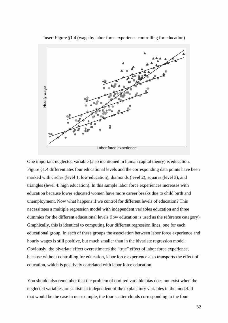
32

Insert Figure §1.4 (wage by labor force experience controlling for education)

One important neglected variable (also mentioned in human capital theory) is education.

Figure §1.4 differentiates four educational levels and the corresponding data points have been

marked with circles (level 1: low education), diamonds (level 2), squares (level 3), and

triangles (level 4: high education). In this sample labor force experiences increases with

education because lower educated women have more career breaks due to child birth and

unemployment. Now what happens if we control for different levels of education? This

necessitates a multiple regression model with independent variables education and three

dummies for the different educational levels (low education is used as the reference category).

Graphically, this is identical to computing four different regression lines, one for each

educational group. In each of these groups the association between labor force experience and

hourly wages is still positive, but much smaller than in the bivariate regression model.

Obviously, the bivariate effect overestimates the “true” effect of labor force experience,

because without controlling for education, labor force experience also transports the effect of

education, which is positively correlated with labor force education.

You should also remember that the problem of omitted variable bias does not exist when the

neglected variables are statistical independent of the explanatory variables in the model. If

that would be the case in our example, the four scatter clouds corresponding to the four

Hou

rly w

age

Labor force experience

33

education levels would be totally parallel (their centers would be on the some vertical line)

and there would be no difference between the slope of the overall and the group-specific

regression lines. Hence, the effect of labor force experience on the hourly wage would be the

same independent of the kind of (bivariate or multiple) regression model.

How to extend the model? Controlling for such “third” factors is an easy task, if we have information about them (like in

the case of education which is available in many surveys). We simply put them as another

independent variable into our regression model. But what about factors that are hard to

measure (“ability” is a prominent example in the context of income analysis) or about which

we have not yet thought about? – First of all, we should make explicit in our models that we

may have neglected certain important explanatory variables. And this applies both to our

time-constant and our time-dependent explanatory variables. Instead of writing them all down

(we don’t know them anyway), we add a time-constant and a time-dependent error component

to our model that include the overall impact of all the unknown factors of each type:

ijijiitkitkitit uzzexxty ++++++++= γγβββ KK 11110 )( (§1.14)

iqjqjijji zzu ,,11 ++++ ++= γγ K summarizes the effect of the q unknown time-constant

explanatory variables and ititskskitkkit vxxe +++= ++++ ,,11 ββ K stands for the s unknown time-

dependent explanatory variables plus all random error )( itv that affects the dependent variable

(e.g., measurement error). iu , the error pertaining to the unit i , is termed unobserved

heterogeneity, because it captures all the variation at the unit level that is not controlled for by

the independent variables in the model. ite , the error pertaining to each single measurement, is

termed idiosyncratic error, because it captures all peculiarities that affect the dependent

variable over time for each unit besides the effects that are already controlled for in the model.

Note in passing that we have dropped the expected value function on the left hand side of the

equation, because (§1.14) models not only the systematic part of the dependent variable but

also the stochastic part )( iti eu + , which we have ignored in the former section §1.5. Note also

that models for categorical data are easily extended in a similar fashion (simply insert the

right hand side of §1.14 into )G( ⋅ in equation §1.9).

34

Some people may view the inclusion of iu and ite only as a notational amendment, since it

does not really let us off the hook of missing information. But it allows us to define the

conditions more concretely that are necessary to achieve unbiased estimates of the parameters

in the model. Since all effects are biased if the corresponding variables are correlated with the

neglected factors (compare the example in Figure §1.4), we must assume – at least at the

present state – that both X and Z are independent of iu and ite to assure unbiasedness of the

parameter estimates. Variables X and Z that meet these criteria are called exogenous in the

econometric literature. We will come back to the issue of exogeneity in Section §1.6.4, when

we know a little bit more about the other specification problems.

When it comes to the question of unbiased estimates, we should also say a few words about

the concrete estimation methods to arrive at these estimates. Models for continuous variables

are usually estimated by ordinary least squares (OLS), while maximum likelihood (ML) is the

preferred method for categorical data.21 The following chapters will show examples of both

estimation methods. Much of the statistical discussion turns around questions of unbiasedness

and efficiency of the estimates and under what conditions these are true for OLS and ML. We

have just stated one of these assumptions, i.e., the exogeneity of X and Z which assures

unbiased estimates. Others will follow. Statistical theory proves that OLS provides unbiased

and efficient estimates given these assumptions, certainly in large samples, but very often also

in small samples. For ML the situation is a little more complicated. The essential assumption

is that the model describes the likelihood of the observed data correctly. Given this

assumption, unbiasedness and efficiency can often be proven only for large samples. If certain

OLS assumptions are violated, but one knows why and how, it is often possible to incorporate

this information into the estimation method and use some kind of generalized least squares

(GLS) algorithm. With ML, however, if the model does not describe the likelihood correctly,

we have no other choice than looking for a better model. All of this may sound like ML has

more disadvantages than OLS. This is difficult to discuss in the abstract, but it is clear that

ML is the much more general estimation method and sometimes we even have no other

choice (e.g., with categorical data).

Why are panel data useful to control for unobserved heterogeneity? First, let us repeat the conclusion from the previous discussion: In order to get unbiased

estimates we have to assume that our explanatory variables are independent of the error terms

21 Naturally, models for continuous data could as well be estimated by ML.

35

(for short, they have to be exogenous). However, stating an assumption without proving it is

true is always a bit disappointing. But with panel data the situation is not hopeless. As we will

shortly see, they are especially suited to deal with at least one of the error terms )( iu , even if

this error term is correlated with the explanatory variables in the model. The necessary

statistical tools are not entirely new. In fact, you will have encountered the fundamental

techniques already during your basic training in statistics.

Let us start with the example on (log) hourly wages. How do we test whether these wages

increased significantly from 1981 to 1982? The increase from 1.513 in 1981 to 1.557 in 1982

(see Table §1.1) could be due to random fluctuations. As you will probably remember, the

significance of this increase can be checked with a T -test for dependent observations. The

corresponding test statistic uses the difference of both arithmetic means and their standard

error:

nyy

yyt y

iiyyyy

2

81,82,2

)()(

81.,82., 2)),Corr(1(ˆwith

ˆ 81.,82.,

81.,82.,

σσ

σ−=

−= −

−

. (§1.15)

For the wage data the standard error is estimated as 0.0195. With an increase of log hourly

wages by 0.0588 points, it results in a highly significant test statistic: 0212.3=t and (one-

sided) 01.0<p .22 Thus, from 1981 to 1982 hourly wages increased significantly by 27 cent or

roughly 6%.

Now consider a simple panel regression model for both years with one time-constant and one

time-dependent explanatory variable and a linear time trend. We drop all observations from

the other years (i.e., make the data a two wave panel study) and write down the regression

equation for each of the two remaining years

iiiii

iiiii

uzexyuzexy

++++⋅+=++++⋅+=

1181,81,111081,

1182,82,111082,

1981:19811982:1982

γβααγβαα

(§1.16)

and then compute their difference

22 Differences between 0212.3=t and )0154.30195(0.0588/0. = are due to rounding.

36

82,82,11182,:FD iii exy Δ+Δ+=Δ βα (§1.17)

The differenced equation does not include the error term iu anymore. Thus, by computing a

regression on the differenced data we get rid of time-constant heterogeneity, whether it is

observed )( 1iz or unobserved )( iu . Consequently, we do not need to bother about potential

correlations between unobserved heterogeneity )( iu and any explanatory variables. First

differences (FD) estimation controls for possible exogeneity bias caused by iu and the

estimated regression coefficients )ˆ(β are unbiased estimates of the “true” effects of the time-

dependent explanatory variables in the model.23 If model (§1.16) includes only a linear time

trend and no explanatory variables, equation (§1.17) reduces to 82,182, ii ey Δ+=Δ α and

0588.0ˆ1 =α will equal the former difference in log hourly wages (with a standard error of

0195.0ˆ1=ασ ). The corresponding t statistic is identical with the test statistic of the former

T -Test. In other words, the T -test for dependent observations known from elementary

statistics is a special case of one important estimation method for panel data.

The formula for the standard error given in (§1.15) is also instructive, because it illustrates our

former statement about the inefficiency of traditional procedures ignoring the serial

dependence in the data. Consider the traditional T -test for independent observations: In this

case we test the difference in (log) hourly wages as if the data were coming from two

independent cross-sections in 1981 and 1982. The nominator of the T statistic remains the

same, but the standard error reduces to nyyy /2ˆ 22)tindependen,( 81.,82.,

σσ =− , which is obviously larger

than the former nyy yiiyy /2)),Corr(1(ˆ 281,82,

2)dependent,( 81.,82.,

σσ ⋅−=− if there is positive serial

correlation )0),(Corr( 81,82, >ii yy . Hence, with a T -test ignoring the dependencies in the data,

our standard errors will be overestimated and we will have less power to falsify our null

hypothesis of no change.

Note also that the nominator of the test statistic (§1.15) is nothing else than the arithmetic

mean of all unit-specific differences 81,82,82, iii yyy −=Δ . Instead of looking at the differences

23 Some other assumptions should be given as well, but these details are not important to understand the main idea of FD estimation. Unfortunately, the FD model (§1.17) also excludes the observed time-constant variables Z . Thus, we have no numerical estimates of their effects, but similar to unobserved heterogeneity iu , their effects on the dependent variable are controlled for (see the discussion in Chapter §).

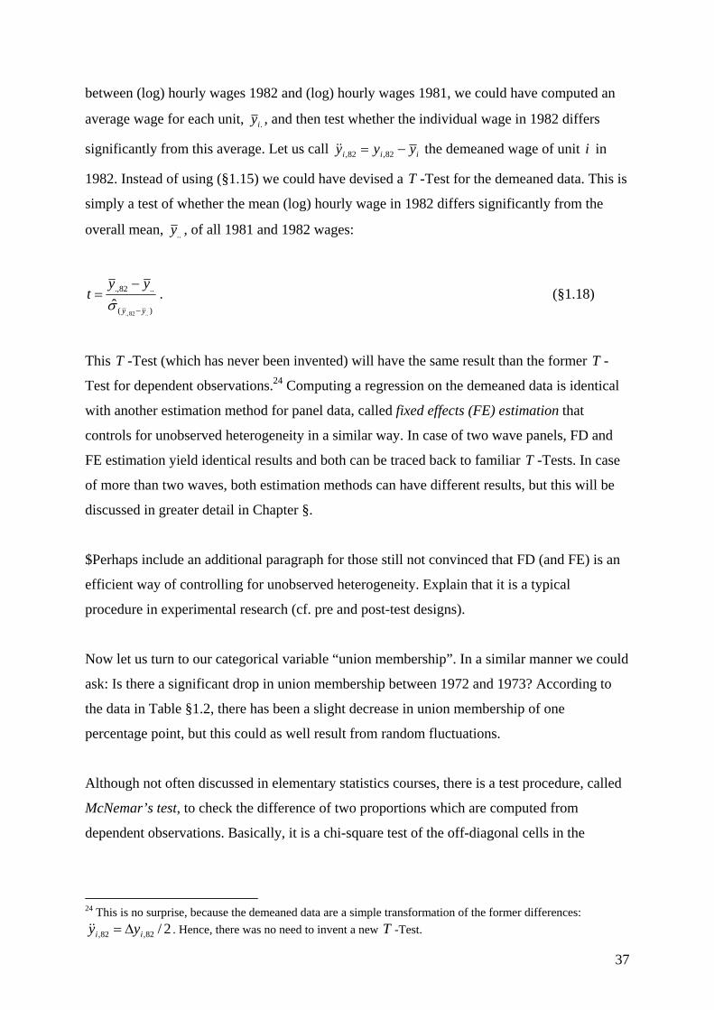
37

between (log) hourly wages 1982 and (log) hourly wages 1981, we could have computed an

average wage for each unit, .iy , and then test whether the individual wage in 1982 differs

significantly from this average. Let us call iii yyy −= 82,82,&& the demeaned wage of unit i in

1982. Instead of using (§1.15) we could have devised a T -Test for the demeaned data. This is

simply a test of whether the mean (log) hourly wage in 1982 differs significantly from the

overall mean, ..y , of all 1981 and 1982 wages:

)(

..82.,

..82.,ˆ yy

yyt

−

−=σ

. (§1.18)

This T -Test (which has never been invented) will have the same result than the former T -

Test for dependent observations.24 Computing a regression on the demeaned data is identical

with another estimation method for panel data, called fixed effects (FE) estimation that

controls for unobserved heterogeneity in a similar way. In case of two wave panels, FD and

FE estimation yield identical results and both can be traced back to familiar T -Tests. In case

of more than two waves, both estimation methods can have different results, but this will be

discussed in greater detail in Chapter §.

$Perhaps include an additional paragraph for those still not convinced that FD (and FE) is an

efficient way of controlling for unobserved heterogeneity. Explain that it is a typical

procedure in experimental research (cf. pre and post-test designs).

Now let us turn to our categorical variable “union membership”. In a similar manner we could

ask: Is there a significant drop in union membership between 1972 and 1973? According to

the data in Table §1.2, there has been a slight decrease in union membership of one

percentage point, but this could as well result from random fluctuations.

Although not often discussed in elementary statistics courses, there is a test procedure, called

McNemar’s test, to check the difference of two proportions which are computed from

dependent observations. Basically, it is a chi-square test of the off-diagonal cells in the

24 This is no surprise, because the demeaned data are a simple transformation of the former differences:

2/82,82, ii yy Δ=&& . Hence, there was no need to invent a new T -Test.

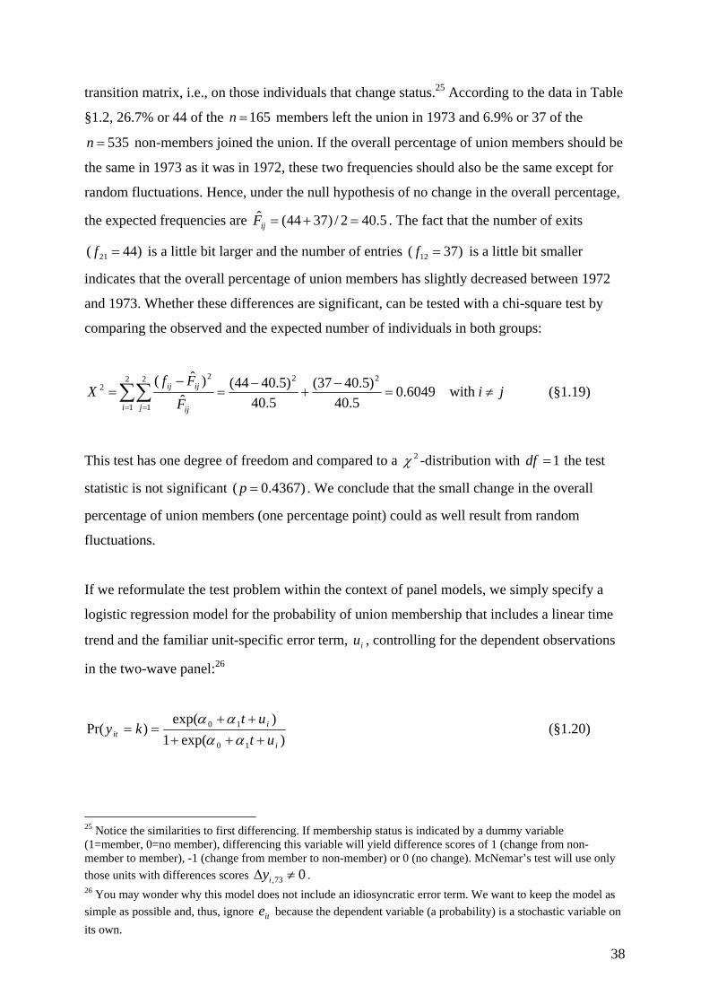
38

transition matrix, i.e., on those individuals that change status.25 According to the data in Table

§1.2, 26.7% or 44 of the 165=n members left the union in 1973 and 6.9% or 37 of the

535=n non-members joined the union. If the overall percentage of union members should be

the same in 1973 as it was in 1972, these two frequencies should also be the same except for

random fluctuations. Hence, under the null hypothesis of no change in the overall percentage,

the expected frequencies are 5.402/)3744(ˆ =+=ijF . The fact that the number of exits

)44( 21 =f is a little bit larger and the number of entries )37( 12 =f is a little bit smaller

indicates that the overall percentage of union members has slightly decreased between 1972

and 1973. Whether these differences are significant, can be tested with a chi-square test by

comparing the observed and the expected number of individuals in both groups:

jiF

FfX

i j ij

ijij ≠=−

+−

=−

=∑∑= =

with6049.05.40

)5.4037(5.40

)5.4044(ˆ

)ˆ( 222

1

2

1

22 (§1.19)

This test has one degree of freedom and compared to a 2χ -distribution with 1=df the test

statistic is not significant 0.4367)( =p . We conclude that the small change in the overall

percentage of union members (one percentage point) could as well result from random

fluctuations.

If we reformulate the test problem within the context of panel models, we simply specify a

logistic regression model for the probability of union membership that includes a linear time

trend and the familiar unit-specific error term, iu , controlling for the dependent observations

in the two-wave panel:26

)exp(1)exp(

)Pr(10

10

i

iit ut

utky

+++++

==αα

αα (§1.20)

25 Notice the similarities to first differencing. If membership status is indicated by a dummy variable (1=member, 0=no member), differencing this variable will yield difference scores of 1 (change from non-member to member), -1 (change from member to non-member) or 0 (no change). McNemar’s test will use only those units with differences scores 073, ≠Δ iy . 26 You may wonder why this model does not include an idiosyncratic error term. We want to keep the model as simple as possible and, thus, ignore ite because the dependent variable (a probability) is a stochastic variable on its own.

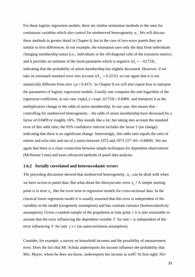
39

For these logistic regression models, there are similar estimation methods to the ones for

continuous variables which also control for unobserved heterogeneity iu . We will discuss

these methods in greater detail in Chapter §, but in the case of two-wave panels they are

similar to first differences. In our example, the estimation uses only the data from individuals

changing membership status (i.e., individuals in the off-diagonal cells of the transition matrix)

and it provides an estimate of the trend parameter which is negative )17330 ˆ( 1 .−=α ,

indicating that the probability of union membership has slightly decreased. However, if we

take its estimated standard error into account )2231.0ˆ(1=ασ we see again that it is not

statistically different from zero )437.0( =p . In Chapter § we will also repeat how to interpret

the parameters of logistic regression models. Usually one computes the anti-logarithm of the

regression coefficient, in our case 8409.0)17330exp( )ˆexp( 1 =−= .α , and interprets it as the

multiplicative change in the odds of union membership. In our case, this means that –

controlling for unobserved heterogeneity – the odds of union membership have decreased by a

factor of 0.8409 or roughly 16%. This sounds like a lot, but taking into account the standard

error of this odds ratio, the 95% confidence interval includes the factor 1 (no change)

indicating that there is no significant change. Interestingly, this odds ratio equals the ratio of

entries and exits into and out of a union between 1972 and 1973 )8409.044/37( = . We see

again that there is a close connection between simple techniques for dependent observations

(McNemar’s test) and more advanced methods of panel data analysis.

1.6.2 Serially correlated and heteroscedastic errors

The preceding discussion showed that unobserved heterogeneity, iu , can be dealt with when

we have access to panel data. But what about the idiosyncratic error ite ? A simple starting

point is to treat ite like the error term in regression models for cross-sectional data. In the

classical linear regression model it is usually assumed that this error is independent of the

variables in the model (exogeneity assumption) and has constant variance (homoscedasticity

assumption). Given a random sample of the population at time point t it is also reasonable to

assume that the error influencing the dependent variable Y for unit i is independent of the

error influencing Y for unit ij ≠ (no autocorrelation assumption).

Consider, for example, a survey on household incomes and the possibility of measurement

error. Does the fact that Mr. Schulz underreports his income influence the probability that

Mrs. Mayer, whom he does not know, underreports her income as well? At first sight: No!

40

Thus, it is a plausible starting point to assume that errors across units (respondents) in cross-

section data are independent. You may object, however, that underreporting income is typical

for certain social groups (e.g., self-employed individuals) and if Schulz and Mayer belong to

the same group it is nevertheless possible that measurement error is similar for both

respondents (and all the other individuals in the same social group). In this case, you should

control for this characteristic by including a suitable indicator into your regression model

(e.g., occupational status, which – by the way – should be included in income equations

anyway as an important predictor).27 Now the assumption of uncorrelated error terms still

holds, at least within the groups defined by the independent variables in your regression

model.

The situation is less easy when you are analyzing panel data, because you observe the same

units repeatedly over time. If there is measurement error, it is not plausible that it happens

only at one point in time. For example, if it is true that self-employed individuals underreport

their incomes, then it is likely that they do it more or less so in each consecutive panel wave.

Hence, the assumption of uncorrelated error terms ite is highly questionable with panel data.

Remember also that ite )( ,,11 ititskskitkk vxx +++= ++++ ββ K includes all unknown time-

dependent factors that affect the dependent variable besides measurement error. In Section

§1.4, when we talked about the serial dependence in our data caused by Z and X , we argued

that the time-dependent independent variables X are not identical each year by definition, but

that they may correlate over time. Consider, for example, the business situation of the

companies that have employed the respondents of our income survey. The business situation

will certainly influence the wages that these companies are able to pay and consequently the

incomes of our respondents. But this information is not easy to obtain for the social scientist

and, therefore, a possible candidate for an unknown time-dependent variable. If the sales

situation correlates over time, so do the error terms ite in our model, which are a function of

theses unknowns.

In sum, the assumption of uncorrelated error terms is at risk with panel data. It is well known

from the analysis of time series data that OLS estimation of linear models is no more efficient

27 If you are not controlling for this variable (let us call it P ), you may have an additional specification problem, if the variables in the model )(X correlate with variable P that predicts measurement error. Necessarily, the variables in the model )(X will correlate with the error term (via the omitted variable P ) and this violates the assumption of independent error terms. All estimated effects for the X will be biased.

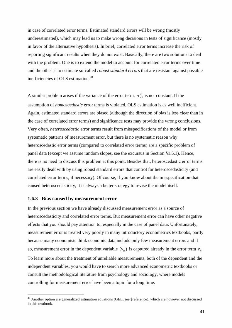
41

in case of correlated error terms. Estimated standard errors will be wrong (mostly

underestimated), which may lead us to make wrong decisions in tests of significance (mostly

in favor of the alternative hypothesis). In brief, correlated error terms increase the risk of

reporting significant results when they do not exist. Basically, there are two solutions to deal

with the problem. One is to extend the model to account for correlated error terms over time

and the other is to estimate so-called robust standard errors that are resistant against possible

inefficiencies of OLS estimation.28

A similar problem arises if the variance of the error term, 2eσ , is not constant. If the

assumption of homoscedastic error terms is violated, OLS estimation is as well inefficient.

Again, estimated standard errors are biased (although the direction of bias is less clear than in

the case of correlated error terms) and significance tests may provide the wrong conclusions.

Very often, heteroscedastic error terms result from misspecifications of the model or from

systematic patterns of measurement error, but there is no systematic reason why

heteroscedastic error terms (compared to correlated error terms) are a specific problem of

panel data (except we assume random slopes, see the excursus in Section §1.5.1). Hence,

there is no need to discuss this problem at this point. Besides that, heteroscedastic error terms

are easily dealt with by using robust standard errors that control for heteroscedasticity (and

correlated error terms, if necessary). Of course, if you know about the misspecification that

caused heteroscedasticity, it is always a better strategy to revise the model itself.

1.6.3 Bias caused by measurement error

In the previous section we have already discussed measurement error as a source of

heteroscedasticity and correlated error terms. But measurement error can have other negative

effects that you should pay attention to, especially in the case of panel data. Unfortunately,

measurement error is treated very poorly in many introductory econometrics textbooks, partly

because many economists think economic data include only few measurement errors and if

so, measurement error in the dependent variable )( itv is captured already in the error term ite .

To learn more about the treatment of unreliable measurements, both of the dependent and the

independent variables, you would have to search more advanced econometric textbooks or

consult the methodological literature from psychology and sociology, where models

controlling for measurement error have been a topic for a long time.

28 Another option are generalized estimation equations (GEE, see $reference), which are however not discussed in this textbook.

42

An important distinction in this context is the distinction between latent and manifest

variables. Our theories focus on the “true” error-free relationships between variables that

represent our theoretical constructs (e.g., human capital, productivity, union commitment).

These are called latent variables. The possibly unreliable indicators of these theoretical

constructs that are provided by social science data (e.g., years of education, earned income,

union membership) are called manifest variables. A simple model assumes that the values of a

manifest variable, say Y , are a linear function of the corresponding latent variable, *Y , plus

some random measurement error:

ititit vyy += *λ (§1.21)

Equation (§1.21) assumes that all variables have been standardized and thus includes no

regression constant. λ is also called the reliability of the manifest variable. It is a measure of

the correlation between the indicator (the manifest variable) and its underlying construct (the

latent variable). In case of categorical variables, measurement error can be modeled as a

process of misclassification, in which only a certain percentage of each category of the latent

variable is assigned correctly to the corresponding category of the manifest variable, while the

rest is erroneously assigned to other categories.

As it turns out, measurement error is much more of a problem for panel than for cross-

sectional data. Although we do not have the space in this textbook to treat models with

measurement error more thoroughly, we would at least provide some advice where models for

panel data may be problematic in case of measurement error. We start with the seemingly

simple case of an unreliable dependent variable (many people will argue that with ite we have

already considered that in our model) and then proceed to the seemingly more difficult case of

unreliable independent variables (because that is poorly treated in the introductory textbook

literature).

Measurement error in the dependent variable

Measurement error in the dependent variable is no problem for cross-sectional data. In that

case it is indeed sufficiently treated in the error term of the model. But for panel data it is a

problem. It can be shown that estimates of true state dependence will be attenuated, i.e.,

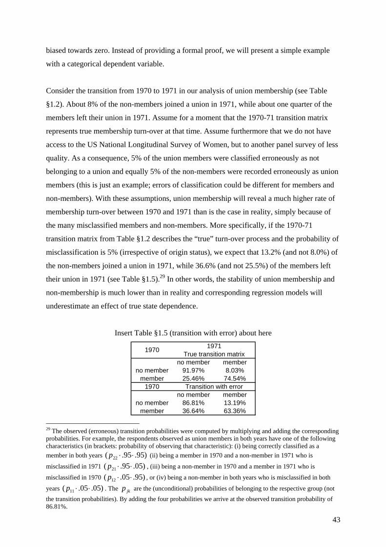
43

biased towards zero. Instead of providing a formal proof, we will present a simple example

with a categorical dependent variable.

Consider the transition from 1970 to 1971 in our analysis of union membership (see Table

§1.2). About 8% of the non-members joined a union in 1971, while about one quarter of the

members left their union in 1971. Assume for a moment that the 1970-71 transition matrix

represents true membership turn-over at that time. Assume furthermore that we do not have

access to the US National Longitudinal Survey of Women, but to another panel survey of less

quality. As a consequence, 5% of the union members were classified erroneously as not

belonging to a union and equally 5% of the non-members were recorded erroneously as union

members (this is just an example; errors of classification could be different for members and

non-members). With these assumptions, union membership will reveal a much higher rate of

membership turn-over between 1970 and 1971 than is the case in reality, simply because of

the many misclassified members and non-members. More specifically, if the 1970-71

transition matrix from Table §1.2 describes the “true” turn-over process and the probability of

misclassification is 5% (irrespective of origin status), we expect that 13.2% (and not 8.0%) of

the non-members joined a union in 1971, while 36.6% (and not 25.5%) of the members left

their union in 1971 (see Table §1.5).29 In other words, the stability of union membership and

non-membership is much lower than in reality and corresponding regression models will

underestimate an effect of true state dependence.

Insert Table §1.5 (transition with error) about here

no member memberno member 91.97% 8.03%

member 25.46% 74.54%1970

no member memberno member 86.81% 13.19%

member 36.64% 63.36%

True transition matrix

Transition with error

19711970

29 The observed (erroneous) transition probabilities were computed by multiplying and adding the corresponding probabilities. For example, the respondents observed as union members in both years have one of the following characteristics (in brackets: probability of observing that characteristic): (i) being correctly classified as a member in both years )95.95.( 22 ⋅⋅p (ii) being a member in 1970 and a non-member in 1971 who is

misclassified in 1971 )05.95.( 21 ⋅⋅p , (iii) being a non-member in 1970 and a member in 1971 who is

misclassified in 1970 )95.05.( 12 ⋅⋅p , or (iv) being a non-member in both years who is misclassified in both

years )05.05.( 11 ⋅⋅p . The jkp are the (unconditional) probabilities of belonging to the respective group (not the transition probabilities). By adding the four probabilities we arrive at the observed transition probability of 86.81%.

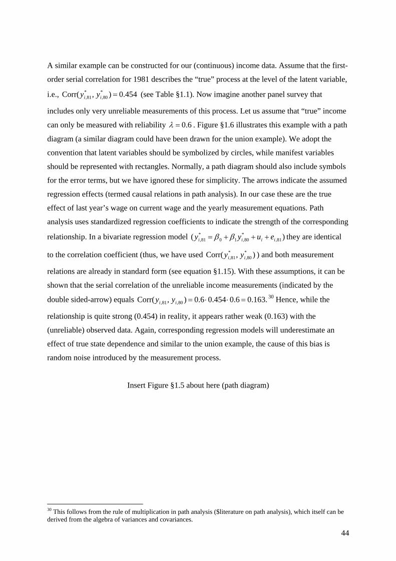
44

A similar example can be constructed for our (continuous) income data. Assume that the first-

order serial correlation for 1981 describes the “true” process at the level of the latent variable,

i.e., 454.0),Corr( *80,

*81, =ii yy (see Table §1.1). Now imagine another panel survey that

includes only very unreliable measurements of this process. Let us assume that “true” income

can only be measured with reliability 6.0=λ . Figure §1.6 illustrates this example with a path

diagram (a similar diagram could have been drawn for the union example). We adopt the

convention that latent variables should be symbolized by circles, while manifest variables

should be represented with rectangles. Normally, a path diagram should also include symbols

for the error terms, but we have ignored these for simplicity. The arrows indicate the assumed

regression effects (termed causal relations in path analysis). In our case these are the true

effect of last year’s wage on current wage and the yearly measurement equations. Path

analysis uses standardized regression coefficients to indicate the strength of the corresponding

relationship. In a bivariate regression model )( 81,*

80,10*

81, iiii euyy +++= ββ they are identical

to the correlation coefficient (thus, we have used ),Corr( *80,

*81, ii yy ) and both measurement

relations are already in standard form (see equation §1.15). With these assumptions, it can be

shown that the serial correlation of the unreliable income measurements (indicated by the

double sided-arrow) equals .163.06.0454.06.0),Corr( 80,81, =⋅⋅=ii yy 30 Hence, while the

relationship is quite strong (0.454) in reality, it appears rather weak (0.163) with the

(unreliable) observed data. Again, corresponding regression models will underestimate an

effect of true state dependence and similar to the union example, the cause of this bias is

random noise introduced by the measurement process.

Insert Figure §1.5 about here (path diagram)

30 This follows from the rule of multiplication in path analysis ($literature on path analysis), which itself can be derived from the algebra of variances and covariances.

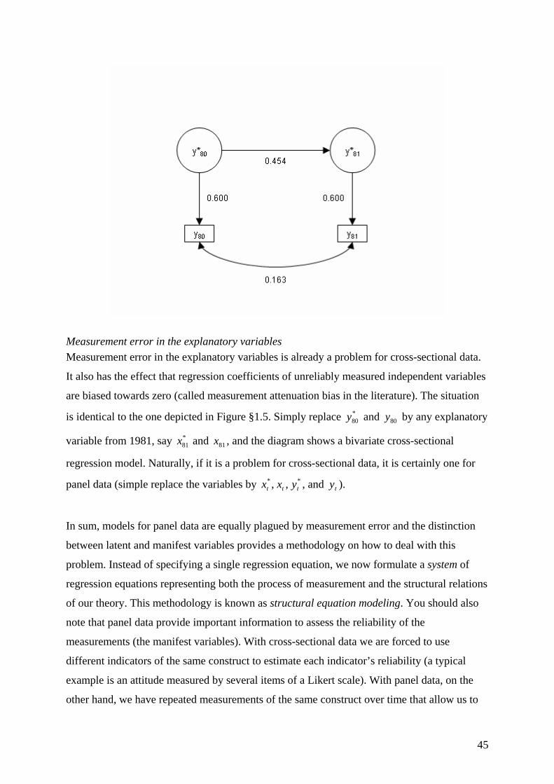
45

Measurement error in the explanatory variables Measurement error in the explanatory variables is already a problem for cross-sectional data.

It also has the effect that regression coefficients of unreliably measured independent variables

are biased towards zero (called measurement attenuation bias in the literature). The situation

is identical to the one depicted in Figure §1.5. Simply replace *80y and 80y by any explanatory

variable from 1981, say *81x and 81x , and the diagram shows a bivariate cross-sectional

regression model. Naturally, if it is a problem for cross-sectional data, it is certainly one for

panel data (simple replace the variables by ** ,, ttt yxx , and ty ).

In sum, models for panel data are equally plagued by measurement error and the distinction

between latent and manifest variables provides a methodology on how to deal with this

problem. Instead of specifying a single regression equation, we now formulate a system of

regression equations representing both the process of measurement and the structural relations

of our theory. This methodology is known as structural equation modeling. You should also

note that panel data provide important information to assess the reliability of the

measurements (the manifest variables). With cross-sectional data we are forced to use

different indicators of the same construct to estimate each indicator’s reliability (a typical

example is an attitude measured by several items of a Likert scale). With panel data, on the

other hand, we have repeated measurements of the same construct over time that allow us to

46

assess their reliability. This is identical to test-retest reliability, one of the classical methods of

reliability estimation.

1.6.4 Summary

This section has been by far the longest in this introduction and thus, it is helpful to

summarize the main conclusions. We have discussed various assumptions that are essential in

getting “good” estimates of our model parameters and we have illustrated – mostly by

examples from elementary statistics – how panel data can be used to relax some of these

assumptions. In order to get unbiased and efficient parameter estimates we have to assume

1. exogeneity, which means that our explanatory variables are independent of all the factors

that we cannot control, either because they are unknown to us or because we have no data

about them. This includes unknown factors on the unit level )( iu as well as unknown

factors on the level of measurements )( ite . Furthermore, unobserved heterogeneity )( iu

and idiosyncratic errors )( ite should be independent of each other. More specifically, we

assume:

0),,,,,,,,,|E( 11111 =itjkiTkiiTii ezzxxxxu KKK

0),,,,,,,,,|E( 11111 =ijkiTkiiTiit uzzxxxxe KKK . (A.1)

2. homoskedasticity, which means that both error terms, iu and ite , have constant variance

across all values of the explanatory variables. In formal terms: 2

11111 ˆ),,,,,,,,|Var( ujkiTkiiTii zzxxxxu σ=KKK

211111 ˆ),,,,,,,,|Var( ejkiTkiiTiit zzxxxxe σ=KKK . (A.2)

3. no autocorrelation, which means that the (time-dependent) idiosyncratic errors are

independent of each other. In formal terms:

stzzxxxxee jkiTkiiTiisit ≠= with0),,,,,,,,|,Corr( 11111 KKK . (A.3)

4. no measurement error, which means that the observed values are identical with the true

values of Y , X and Z .

There are also some other more technical assumptions, which will be discussed in the

following chapters. The most important assumption is the exogeneity assumption, because it

assures unbiasedness of the parameter estimates (besides the fourth assumption of perfectly

reliable measurements). What (A.1) says is that each error term is zero on average, once we

control for all the other variables in the model. Homoskedastic and uncorrelated error terms

(assumptions 2 and 3) guarantee efficient estimates and unbiased standard errors. Similar to

47

(A.1), (A.2) and (A.3) make a statement about the variance and the autocorrelation of the

error terms given the other variables in the model.

Why does it make sense to specify all the assumptions in terms of conditional expected

values, variances, and correlations? Well, as you may remember from our former discussion,

biased estimates, heteroscedastic error terms and autocorrelated errors may result from

misspecifications of the model. The effect of labor force experience was overestimated, when

we did not control for education. Autocorrelated errors in an analysis of labor income may

result from systematic under- or overreporting of certain groups (e.g., self-employed

individuals). And so on. These problems do not exist, if we specify our models correctly (i.e.,

include an education variable or a dummy for self-employment). Thus our assumptions 1-4

are conditional on the model we are estimating.

You may also wonder, why these conditions mention all the T measurements of each time-

dependent explanatory variable (e.g., iTit xx 11 ...,, ). This is due to the fact that we are dealing

with panel data. With one cross-section of data, it is not necessary to consider what happens

in other time periods. However, with panel data past and future values of the explanatory

variables can affect the dependent variable and thus the error terms. This more comprehensive

definition of (A.1) is also known as the assumption of strict exogeneity (as opposed to

contemporaneous exogeneity in the case of cross-section data). Strict exogeneity is at stake

when we are analyzing models with lagged dependent variables and feedback processes (non-

recursive models).

Finally, as we have seen in Section §1.6.1, the first part of assumption (A.1) is not a real

problem with panel data, because repeated observations of the same units allow us to control

for unobserved heterogeneity iu , even if it is correlated with the variables in the model. This

is one of the great advantages of panel data over cross-sectional data. We have learned that

there are special estimation methods for this problem (first differences, fixed effects) and in

the following chapters we will study these methods in greater detail. Furthermore, if both

parts of assumption (A.1) hold, panel data give us the opportunity to estimate the effects of

the explanatory variables much more efficiently than with cross-sectional data. However, it is

an interesting question what happens with FD, FE and other panel estimation methods, when

assumptions 2-4 do not hold. This discussion is deferred to the following chapters.

48

1.7 An outlook on the following chapters and the literature As already mentioned in the introduction, it is difficult for the novice user to get some basic

orientation in the field of panel data analysis. This has also to do with the different disciplines

working in the field, which all have their own methodological traditions. This diversity has its

pros and cons. An advantage is certainly that you find many good textbooks on panel data

analysis in your discipline that tie in with your methodological training. But at a certain point,

you will come across (seemingly) different panel data methods and ask yourself whether it is

a new methodology or something that you already know. Often you will have the feeling that

it is only different people talking about the same problem but using different terminologies.

This lack of interdisciplinary communication and generality is certainly a disadvantage.

Nevertheless it useful to have a look at the different methodological traditions and their

literature ($the following bullet list could be worked out and augmented by literature

recommendations, but could be dropped as well):

• Econometrics: regression analysis, time-series analysis. Mostly focusing on continuous

data (often on the aggregate level). However, with the advent of large household panels

also focusing on categorical variables. Specific contribution: FD, FE and other estimation

methods for the linear model.

• Psychology: analysis of variance. Mostly focusing on experimental data (continuous Y ,

categorical (sometimes continuous) X and Z ). Specific contribution: analysis of repeated

measurements, variance components models.

• Pedagogy/Psychology (and increasingly internationally comparative survey researchers):

analyzing grouped data (students within classes within schools, respondents within

regions within countries). Specific contribution: hierarchical linear modeling.

• Political Science: mostly focusing on continuous data on the aggregate level. Specific

contribution: methods for TSCS data (macro panels).

• Sociology and Life Sciences: analyzing duration data and events. Specific contribution:

survival and event history data.

• Micro panel researchers (Sociologists, Political Scientists): analyzing tabular data

(transition matrices). Specific contribution: Markov models.

• Sociology/Psychology: analyzing (unreliable) attitude data. Specific contribution:

structural equation modeling.

In this introduction we have attempted to capture some of the strands of these methodologies.

By making a distinction between the kind of (continuous or categorical) dependent variable

49

you are interested in and by proposing to analyze its level or its change, we hoped to give

some basic orientation. In the following chapters we will focus on models for the level and

change of continuous variables (extending equation §1.3; see Chapter §), for the level of

categorical variables (extending equation §1.9; see Chapter §) and for the change of

categorical variables (extending equation §1.13; see Chapter §). Because this is an

introductory textbook, we will not focus on systems of regression equations (that are used to

model non-recursive relationships YX ↔ ) and we will not discuss models that distinguish

latent and manifest variables (that are used to model measurement error). $Refer the reader to

some textbooks related to these more advanced methods.

References Menard, Scott (2002): Longitudinal Research. Quantitative Applications in the Social Sciences 76. Newbury Park / London / New Delhi: Sage Publications Rabe-Hesketh, Sophia/ Skrondal, Anders (2005): Multilevel and Longitudinal Modeling Using Stata. College Station, Texas: Stata Press.