COUNTEREXAMPLES TOTHE EISENBUD-GOTO REGULARITY CONJECTURE

JASON MCCULLOUGH AND IRENA PEEVA

Abstract. Our main theorem shows that the regularity of non-degenerate ho-mogeneous prime ideals is not bounded by any polynomial function of the degree;this holds over any field k. In particular, we provide counterexamples to thelongstanding Regularity Conjecture, also known as the Eisenbud-Goto Conjec-ture (1984). We introduce a method which, starting from a homogeneous ideal I,produces a prime ideal whose projective dimension, regularity, degree, dimension,depth, and codimension are expressed in terms of numerical invariants of I. Themethod is also related to producing bounds in the spirit of Stillman’s Conjecture,recently solved by Ananyan-Hochster.

1. Introduction

Hilbert’s Syzygy Theorem provides a nice upper bound on the projective dimensionof homogeneous ideals in a standard graded polynomial ring: projective dimensionis smaller than the number of variables. In contrast, there is a doubly exponentialupper bound on the Castelnuovo-Mumford regularity in terms of the number ofvariables and the degrees of the minimal generators. It is the most general boundon regularity in the sense that it requires no extra conditions. The bound is nearlysharp since the Mayr-Meyer construction leads to examples of families of ideals at-taining doubly exponential regularity. On the other hand, for reduced, irreducible,smooth (or nearly smooth) projective varieties over an algebraically closed field,regularity is well controlled by several upper bounds in terms of the degree, codi-mension, dimension or degrees of defining equations. As discussed in the influentialpaper [BM] by Bayer and Mumford, “the biggest missing link” between the gen-eral case and the smooth case is to obtain a “decent bound on the regularity ofall reduced equidimensional ideals”. The longstanding Regularity Conjecture 1.2,by Eisenbud-Goto [EG] (1984), predicts a linear bound in terms of the degree fornon-degenerate prime ideals over an algebraically closed field. In subsection 1.7 wegive counterexamples to the Regularity Conjecture 1.2.

2010 Mathematics Subject Classification. Primary: 13D02.Key words and phrases. Syzygies, Free Resolutions, Castelnuovo-Mumford Regularity.Peeva is partially supported by NSF grant DMS-1406062.

1

Our main Theorem 1.9 is much stronger and shows that the regularity of non-degenerate homogeneous prime ideals is not bounded by any polynomial functionof the degree; this holds over any field k (the case k = C is particularly important).We provide a family of prime ideals P

r

, depending on a parameter r 2 N, whosedegree is singly exponential in r and whose regularity is doubly exponential in r. Forthis purpose, we introduce an approach, outlined in subsection 1.5, which startingfrom a homogeneous ideal I, produces a prime ideal P whose projective dimension,regularity, degree, dimension, depth, and codimension are expressed in terms ofnumerical invariants of I.

1.1 Motivation and Conjectures. This subsection provides an overview of reg-ularity conjectures and related results. We consider a standard graded polynomialring U = k[z1, . . . , zp] over a field k, where all variables have degree one. Projec-tive dimension and regularity are well-studied numerical invariants that measurethe size of a Betti table. Let L be a homogeneous ideal in the ring U , and let�ij

(L) = dimk

TorUi

(L, k)j

be its graded Betti numbers. The projective dimension

pd(L) = maxn

i�

�

�

�ij

(L) 6= 0o

is the index of the last non-zero column of the Betti table �(L) :=�

�i,i+j

(L)�

, andthus it measures its width. The height of the table is measured by the index ofthe last non-zero row and is called the (Castelnuovo-Mumford) regularity of L; it isdefined as

reg(L) = maxn

j�

�

�

�i, i+j

(L) 6= 0o

.

By [EG, Theorem 1.2], (see also [Pe, Theorem 19.7]) for any q � reg(L), the trun-cated ideal L�q

is generated in degree q and has a linear minimal free resolution.A closely related invariant maxdeg(L) is the maximal degree of an element in aminimal system of homogeneous generators of L. Note that maxdeg(L) reg(L).

Alternatively, regularity can be defined using local cohomology, see for example,the expository papers [Ch, Ei] and the books [Ei2, La2].

Hilbert’s Syzygy Theorem (see for example, [Ei3, Corollary 19.7] or [Pe, Theo-rem 15.2]) provides a nice upper bound on the projective dimension of L :

pd(L) < p.

However, the general (not requiring any extra conditions) regularity bound is doublyexponential:

reg(L) (2maxdeg(L))2p�2

.

It is proved by Bayer-Mumford [BM] (using results in Giusti [Gi] and Galligo [Ga]) ifchar(k) = 0, and by Caviglia-Sbarra [CS] in any characteristic. This bound is nearlythe best possible, due to examples based on the Mayr-Meyer construction [MM]; for

2

example, there exists an ideal L in 10r + 1 variables for which maxdeg(L) = 4 and

reg(L) � 22r

by [BM, Proposition 3.11]. Other versions of the Mayr-Meyer ideals were con-structed by Bayer-Stillman [BS] and Koh [Ko].

Still more examples of ideals with high regularity have been constructed byCaviglia, Chardin-Fall, and Ullery [Ca, CF, Ul]. For more details about regularity,we refer the reader to the expository papers [BM, Ch, Ei] and the books [Ei2, La2].

In sharp contrast, a much better bound is expected if L = I(X) is the van-ishing ideal of a geometrically nice projective scheme X ⇢ Pp�1

k

. The followingelegant bound was conjectured by Eisenbud, Goto, and others, and has been verychallenging.

The Regularity Conjecture 1.2. (Eisenbud-Goto [EG], 1984) Suppose that thefield k is algebraically closed. If L ⇢ (z1, . . . , zp)

2 is a homogeneous prime ideal inU , then

(1.3) reg(L) deg(U/L)� codim(L) + 1 ,

where deg(U/L) is the multiplicity of U/L (also called the degree of U/L, or thedegree of X), and codim(L) is the codimension (also called height) of L.

The condition that L ⇢ (z1, . . . , zp)2 is equivalent to requiring that X is not con-

tained in a hyperplane in Pp�1k

. Prime ideals that satisfy this condition are callednon-degenerate.

The Regularity Conjecture holds if U/L is Cohen-Macaulay by [EG]. It isproved for curves by Gruson-Lazarsfeld-Peskine [GLP], completing classical workof Castelnuovo. It also holds for smooth surfaces by Lazarsfeld [La] and Pinkham[Pi], and for most smooth 3-folds by Ran [Ra]. In the smooth case, Kwak [Kw]gave bounds for regularity in dimensions 3 and 4 that are only slightly worse thanthe optimal ones in the conjecture; his method yields new bounds up to dimension14, but they get progressively worse as the dimension goes up. Other special casesof the conjecture and also similar bounds in special cases are proved by Brodmann[Br], Brodmann-Vogel [BV], Eisenbud-Ulrich [EU], Herzog-Hibi [HH], Hoa-Miyazaki[HM], Kwak [Kw2], and Niu [Ni].

The following variations of the Regularity Conjecture have been of interest:Eisenbud and Goto further conjectured that the hypotheses in 1.2 can be weak-

ened to say that X is reduced and connected in codimension 1. This was proved forcurves by Giaimo [Gia]. Examples show that the hypotheses cannot be weakenedmuch further: The regularity of a reduced equidimensional X cannot be boundedby its degree, as [EU, Example 3.1] gives a reduced equidimensional union of twoirreducible complete intersections whose regularity is much larger than its degree.

3

Example 3.11 in [Ei] shows that there is no bound on the regularity of non-reducedhomogeneous ideals in terms of multiplicity, even for a fixed codimension. See [Ei2,Section 5C, Exercise 4] for an example showing that the hypothesis that the field k

is algebraically closed is necessary.In 1988 Bayer and Stillman [BS, p. 136], made the related conjecture that the

regularity of a reduced scheme over an algebraically closed field is bounded by itsdegree (which is the sum of the degrees of its components). This holds if L is thevanishing ideal of a finite union of linear subspaces of Pp�1

k

by a result of Derksen-Sidman [DS].

It is a very basic problem to get an upper bound on the degrees of the definingequations of an irreducible projective variety. The following weaker form of theRegularity Conjecture provides an elegant bound.

Conjecture 1.4. (Folklore Conjecture) Suppose that the field k is algebraicallyclosed. If L is a homogeneous non-degenerate prime ideal in U , then

maxdeg(L) deg(U/L) .

1.5. Our Approach. Fix a polynomial ring S = k[x1, . . . , xn] over a field k with astandard grading defined by deg(x

i

) = 1 for every i. As discussed above, there existexamples of homogeneous ideals with high regularity (for example, based on theMayr-Meyer construction), but they are not prime. Motivated by this, we introducea method which, starting from a homogeneous ideal I, produces a prime ideal Pwhose projective dimension, regularity, maxdeg, multiplicity, dimension, depth, andcodimension are expressed in terms of numerical invariants of I. The method hastwo ingredients: Rees-like algebra and Step-by-step Homogenization.

In Section 3, we consider the prime ideal Q of defining equations of the Rees-likealgebra S[It, t2]. This was inspired by Hochster’s example in [Be] which, startingwith a family of three-generated ideals in a regular local ring, produces prime idealswith embedding dimension 7, Hilbert-Samuel multiplicity 2, and arbitrarily manyminimal generators. In contrast to the usual Rees algebra, whose defining equa-tions are di�cult to find in general (see for example [Hu], [KPU]), those of theRees-like algebra are given explicitly in Proposition 3.2. Furthermore, one can ob-tain the graded Betti numbers of Q using a mapping cone resolution described inTheorem 3.10.

We introduce Step-by-step Homogenization in Section 4. The ideal Q is ho-mogeneous but in a polynomial ring that is not standard graded. We change thedegrees of the variables to 1 and homogenize the ideal; we do this one variable at atime, in order to not drop the degrees of the defining equations. One usually needsto homogenize a Grobner basis in order to obtain a generating set of a homoge-nized ideal, but we show that in our case it su�ces to homogenize a minimal set of

4

generators. Our Step-by-step Homogenization method is expressed in Theorem 4.5,which can be applied to any non-degenerate prime ideal that is homogeneous in apositively graded polynomial ring in order to obtain a homogeneous prime ideal in astandard graded polynomial ring. Its key property is the preservation of the gradedBetti numbers, which usually change after homogenization. Applying this to theideal Q we produce a prime ideal P , by Proposition 4.8.

A set of generators of P is defined in Construction 2.4, and we prove in Propo-sition 2.9 that it is minimal. The key and striking property of the construction ofthe ideal P is that it has a nicely structured minimal free resolution (coming fromthe minimal free resolution of Q), which makes it possible to express its regularity,multiplicity, and other invariants in terms of invariants of I. We prove the followingproperties of P :

Theorem 1.6. Let k be any field. Let I be an ideal generated minimally by homo-geneous elements f1, . . . , fm (with m � 2) in the standard graded polynomial ringS = k[x1, . . . , xn].

The ideal P , defined in Construction 2.4, is homogeneous in the standard gradedpolynomial ring

R = S[y1, . . . , ym, u1, . . . , um, z, v]

with n+2m+2 variables. It is minimally generated by the elements listed in (2.5) and(2.6), (by Proposition 2.9). It is prime and non-degenerate, (by Proposition 4.8).Furthermore:

(1) The maximal degree of a minimal generator of P is

maxdeg(P ) = max

⇢

1 + maxdeg�

SyzS1 (I)�

, 2�

maxdeg(I) + 1�

�

.

(2) The multiplicity of R/P is

deg(R/P ) = 2m

Y

i=1

�

deg(fi

) + 1�

.

(3) The Castelnuovo-Mumford regularity, the projective dimension, the depth,the codimension, and the dimension of R/P are:

reg(R/P ) = reg(S/I) + 2 +m

X

i=1

deg(fi

)

pd(R/P ) = pd(S/I) +m� 1

depth(R/P ) = depth(S/I) +m+ 3

codim(P ) = m

dim(R/P ) = m+ n+ 2 .5

Property (1) holds by Corollary 2.10. Property (2) holds by Theorem 5.2.The properties listed in (3) are proved in Section 5. Above, we used reg(R/P ) =reg(P ) � 1 and pd(R/P ) = pd(P ) + 1. Since depth(R/P ) � m + 3, we may useBertini’s theorem, see [Fl], to reduce the number of variables by at least m+ 2 andthus obtain a prime ideal P 0 in a polynomial ring R0 with at most n+m variables,instead of n+ 2m+ 2 variables, and with dim(R0/P 0) n. Note that factoring outlinear homogeneous non-zerodivisors preserves projective dimension, regularity, anddegree.

1.7. Counterexamples and the Main Theorem. We provide the followingcounterexamples to the Regularity Conjecture 1.2. They are also counterexamplesto the weaker Conjecture 1.4 and the Bayer-Stillman Conjecture. For this, we useproperties (1) and (2) in Theorem 1.6.

Counterexamples 1.8. The counterexamples in (1) and (2) hold over any field k.

(1) For r � 1, Koh constructed in [Ko] an ideal Ir

generated by 22r� 3 quadricsand one linear form in a polynomial ring with 22r � 1 variables, and such

that maxdeg(Syz1(Ir)) � 22r�1

. His ideals are based on the Mayr-Meyerconstruction in [MM]. By Theorem 1.6, I

r

leads to a homogeneous primeideal P

r

(in a standard graded polynomial ring Rr

) whose multiplicity andmaxdeg are:

deg(Rr

/Pr

) 4 · 322r�3 < 422r�2 < 250r

maxdeg(Pr

) � 22r�1

+ 1 > 22r�1

.

Therefore, Conjecture 1.4 predicts

22r�1

+ 1 4 · 322r�3 ,

which fails for r � 9. Moreover, the di↵erence

reg(Pr

)� deg(Rr

/Pr

) � maxdeg(Pr

)� deg(Rr

/Pr

) > 22r�1

� 250r

can be made arbitrarily large by choosing a large r.(2) Alternatively, we can use the Bayer-Stillman example in [BS, Theorem 2.6]

instead of Koh’s example. For r � 1, they constructed a homogeneous ideal Ir

(using d = 3 in their notation) generated by 7r+5 forms of degree at most 5 ina polynomial ring with 10r+11 variables and such that maxdeg(Syz1(Ir)) �32

r�1

. The example is based on the Mayr-Meyer construction in [MM]. ByTheorem 1.6, I

r

leads to a homogeneous prime ideal Pr

whose multiplicity

is deg(Rr

/Pr

) 2 · 67r+5 and with maxdeg(Pr

) � 32r�1

+ 1. Therefore,

Conjecture 1.4 predicts 32r�1

+ 1 2 · 67r+5, which fails for r � 8.6

(3) In Section 4, we give two examples of 3-dimensional projective varieties in P5

for which the Regularity Conjecture 1.2 fails. These examples cannot proveTheorem 1.9 but are small enough to be computable with Macaulay2 [M2].

We remark that from Counterexamples 1.8(1),(2) it follows that we can obtaincounterexamples using the Rees algebras S[I

r

t] (instead of the Rees-like algebrasS[I

r

t, t2]); this is proved in [CMPV]. In that paper we also construct counterexam-ples which do not rely on the Mayr-Meyer construction.

What next? The bound in the conjecture is very elegant, so it is certainly ofinterest to study if it holds when we impose extra conditions on the prime ideal.

Suppose char(k) = 0 andX ⇢ Pp�1k

is a smooth variety. In this case the Regular-ity Conjecture is open and Kwak-Park [KP] and Noma [No] reduced it to the Castel-nuovo’s Normality Conjecture that X is r-normal for all r � deg(X) � codim(X).However, other bounds are known. Bertram-Ein-Lazarsfeld [BEL] obtained an im-portant bound that implies

regX 1 + (s� 1)codimX

if X is cut out scheme-theoretically by equations of degree s. Later this boundwas proved by Chardin-Ulrich [CU] for X satisfying weaker conditions. See [Ch2]for an overview. These results were generalized in [DE] to a large class of pro-jective schemes. On the other hand, Mumford proved in the appendix of [BM,Theorem 3.12] that if X is reduced, smooth, and pure dimensional then

regX (dimX + 1)(degX � 2) + 2 .

Note that the above bounds are di↵erent in flavor than the Regularity Conjecture:they are not linear in the degree (or the degree of the defining equations) since thereis a coe�cient involving the dimension or codimension.

In [BM] Bayer and Mumford pointed out that the main missing piece of in-formation between the general case and the geometrically nice smooth case is thatwe do not have yet a reasonable bound on the regularity of all reduced equidi-mensional ideals. Thus, instead of imposing extra conditions on the ideals we mayweaken the bound, which is linear in the Regularity Conjecture. If the residue fieldk is algebraically closed and L is a non-degenerate prime ideal, then deg(U/L) �1+codim(U/L) (see for example, [EG, p. 112]). So instead of a bound on regularityinvolving multiplicity and codimension, we could look for a bound in terms of themultiplicity alone. Counterexamples 1.8(1)(or 2) prove the main result in our paper:

Main Theorem 1.9. Over any field k (the case k = C is particularly important),the regularity of non-degenerate homogeneous prime ideals is not bounded by anypolynomial function of the multiplicity, i.e., for any polynomial ⇥(x) there exists anon-degenerate homogeneous prime ideal L in a standard graded polynomial ring V

over the field k such that reg(L) > ⇥�

deg(V/L)�

.7

Proof. In the notation and under the assumptions of Counterexmaples 1.8(1), wehave

reg(Pr

) > 22r�1

> 21/2·deg(Rr/Pr)1/50

=⇣p

2⌘deg(Rr/Pr)

1/50

.

The function f(x) =�

p2�

x

1/50

is not bounded above by any polynomial in x. ⇤

It is natural to wonder if there exists any bound in terms of the multiplicity. In[CMPV] we prove the existence of such a bound using the recent result of Ananyan-Hochster [AH2] that Stillman’s Conjecture holds. However, the bound obtained inthis way is very large.

Question 1.10. Suppose the field k is algebraically closed. What is an optimalfunction �(x) such that reg(L) �(deg(L)) for any non-degenerate homogeneousprime ideal L in a standard graded polynomial ring over k?

In the spirit of [BS] it would be nice if �(x) is singly exponential.Next we will explain how Question 1.10 is related to Stillman’s Conjecture,

which asks whether there exists an upper bound on the regularity of homogeneousideals generated by m forms of degrees a1, . . . , am (independent of the number ofvariables). Let I be an ideal in a standard graded polynomial ring S over a field K

minimally generated by homogeneous forms of degrees a1, . . . , am. We may enlargethe base field K to an algebraically closed field k without changing the regularity.Let �(x) be a function such that reg(L) �(deg(L)) for any non-degenerate homo-geneous prime ideal L in a standard graded polynomial ring over k. Let P be theprime ideal associated to I according to our method, and apply Theorem 1.6. Then

reg(I) reg(P ) �(deg(R/P )) = �

2m

Y

i=1

(ai

+ 1)

!

.

Thus, � (2Q

m

i=1 (ai + 1)) provides a bound on the regularity in terms of the degreesa1, . . . , am of the generators.

Bounds for Stillman’s Conjecture which are better than those obtained in [AH2]were obtained for all ideals generated by quadrics by Ananyan-Hochster in [AH].They have also announced bounds in the cases of generators of degree at mostthree, or generators of degree at most four and char(k) 6= 2. See the expositorypapers [FMP, MS] for a discussion of other results in this direction.

There is an equivalent form of Stillman’s Conjecture that replaces projectivedimension by regularity; the equivalence of the two conjectures was proved by Cav-iglia. Motivated by this, we discuss projective dimension of prime ideals in Section 6.Theorem 6.2 provides an analogue to Theorem 1.9.

8

2. Definition of the ideal P , starting from a given ideal I

In this section, we introduce notation which will be used in the rest of the paper.Starting form a homogeneous ideal I, we write generators for a new ideal, which wedenote by P . We will study the properties of P in the next sections.

Notation 2.1. If N is a graded module and p 2 Z, denote by N(�p) the shiftedmodule for which N(�p)

i

= Ni�p

for all i.If (V, d) is a complex, we write V[�p] for the shifted complex with V[�p]

i

=V

i+p

and di↵erential (�1)pd.

For a finitely generated graded U -module N , we denote by SyzUi

(N) the ith

syzygy module.

Assumptions and Notation 2.2. Consider the polynomial ring

S = k[x1, . . . , xn]

over a field k with a standard grading defined by deg(xi

) = 1 for every i. Let I be ahomogeneous ideal minimally generated by forms f1, . . . , fm of degrees a1, . . . , am,where m � 2. We denote by (F, dF ) the minimal graded S-free resolution of

SyzS2 (S/I) = SyzS1 (I). Thus the minimal graded S-free resolution of S/I has theform

F0 : F[2]d

F0 =(cij)�������! F�1 := S(�a1)� · · ·� S(�a

m

)d

F�1=(f1 ... fm)

�����������! F�2 := S ,

and in particular F is a truncation of F0.Denote by ⇠1, . . . , ⇠m a homogeneous basis of F�1 = S(�a1)� · · ·�S(�a

m

) such

that dF�1(⇠i) = fi

for every i. Fix a homogeneous basis µ1, . . . , µrank F0of F0 that

is mapped by the di↵erential dF0 to a homogeneous minimal system of generatorsof Ker(dF�1). Let C = (c

ij

) be the matrix of the di↵erential dF0 in these fixed

homogeneous bases. Thus SyzS1 (I) is generated by the elements

(2.3)

(

m

X

i=1

cij

⇠i

�

�

�

�

�

1 j rank (F0)

)

.

In matrix form, these elements correspond to the entries in the matrix product(⇠1, ⇠2, . . . , ⇠m)C .

Construction 2.4. In the notation and under the assumptions of 2.2, we will definean ideal P . The motivation for this construction is outlined in subsection 1.5 of theIntroduction. We consider the standard graded polynomial ring

R = S[y1, . . . , ym, u1, . . . , um, z, v] = k[x1, . . . , xn, y1, . . . , ym, u1, . . . , um, z, v] .

Let P be the ideal generated by

(2.5)�

yi

yj

uaii

uaj

j

� zvfi

fj

�

� 1 i, j m

9

and

(2.6)

(

m

X

i=1

cij

yi

uaii

�

�

�

�

�

1 j rank (F0)

)

.

The degrees of these generators are

deg(yi

yj

uaii

uaj

j

� zvfi

fj

) = deg(fi

) + deg(fj

) + 2

deg

✓

m

X

i=1

cij

yi

uaii

◆

= 1 + deg

✓

m

X

i=1

cij

⇠i

◆

,(2.7)

whereP

m

i=1 cij

⇠i

belongs to the minimal system of homogeneous generators (2.3)

of SyzS1 (I).The ideal P is homogeneous. It is non-degenerate since there are no linear forms

among the generators listed above.

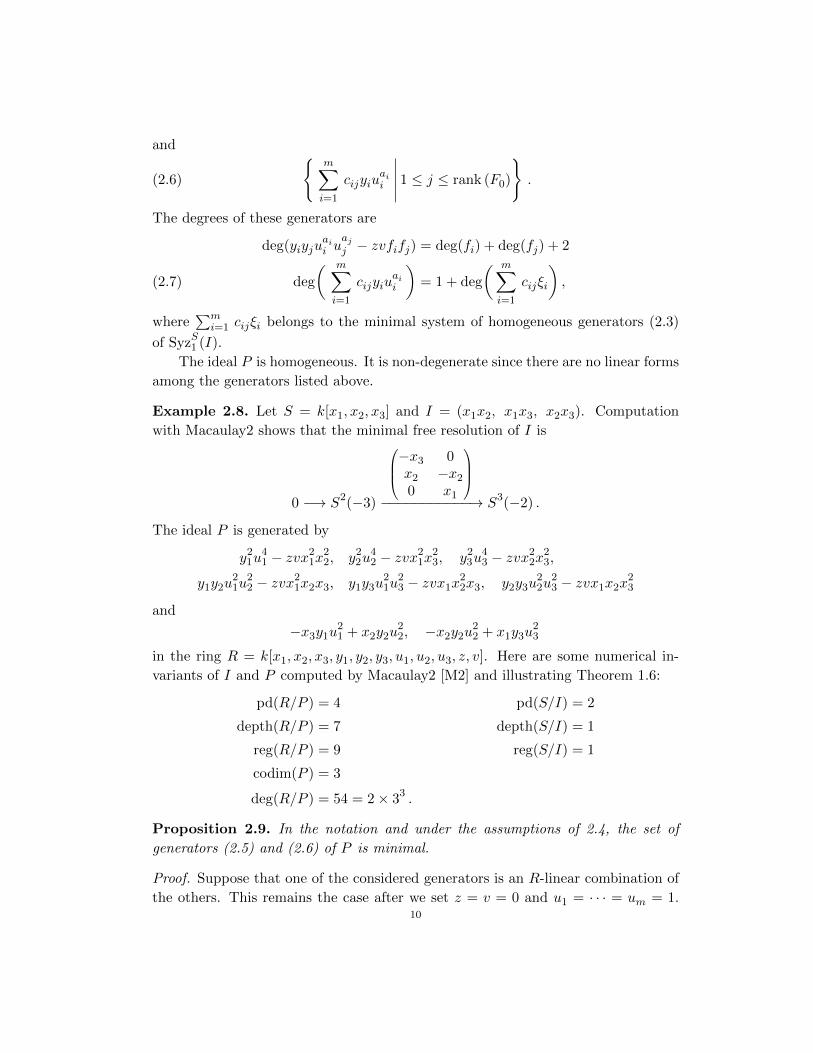
Example 2.8. Let S = k[x1, x2, x3] and I = (x1x2, x1x3, x2x3). Computationwith Macaulay2 shows that the minimal free resolution of I is

0 �! S2(�3)

0

BB@

�x3 0x2 �x20 x1

1

CCA

�����������! S3(�2) .

The ideal P is generated by

y21u41 � zvx21x

22, y22u

42 � zvx21x

23, y23u

43 � zvx22x

23,

y1y2u21u

22 � zvx21x2x3, y1y3u

21u

23 � zvx1x

22x3, y2y3u

22u

23 � zvx1x2x

23

and

�x3y1u21 + x2y2u

22, �x2y2u

22 + x1y3u

23

in the ring R = k[x1, x2, x3, y1, y2, y3, u1, u2, u3, z, v]. Here are some numerical in-variants of I and P computed by Macaulay2 [M2] and illustrating Theorem 1.6:

pd(R/P ) = 4 pd(S/I) = 2

depth(R/P ) = 7 depth(S/I) = 1

reg(R/P ) = 9 reg(S/I) = 1

codim(P ) = 3

deg(R/P ) = 54 = 2⇥ 33 .

Proposition 2.9. In the notation and under the assumptions of 2.4, the set ofgenerators (2.5) and (2.6) of P is minimal.

Proof. Suppose that one of the considered generators is an R-linear combination ofthe others. This remains the case after we set z = v = 0 and u1 = · · · = u

m

= 1.10

Thus, an element g in one of the sets

A :=�

yi

yj

| 1 i, j m

B :=

(

m

X

i=1

cij

yi

�

�

�

�

�

1 j rank (F0)

)

is an S[y1, . . . , ym]-linear combination of the other elements in these sets. We willwork over the ring S[y1, . . . , ym].

By Construction 2.2, we have cij

2 (x1, . . . , xn). Hence, B ⇢ (x1, . . . , xn), andit follows that g /2 A.

Let g 2 B. Since A generates (y1, . . . , ym)2 it follows that g is an S-linearcombination of the elements in B. This contradicts the fact that the columns of thematrix C (in the notation of Construction 2.2) form a minimal system of generators

of SyzS1 (I).

Recall from the Introduction that for a finitely generated graded module N

(over a positively graded polynomial ring), we denote by maxdeg(N) the maximaldegree of an element in a minimal system of homogeneous generators of N .

Corollary 2.10. In the notation and under the assumptions of 2.4,

maxdeg(P ) = max

⇢

1 + maxdeg�

SyzS1 (I)�

, 2�

maxdeg(I) + 1�

�

Proof. Apply (2.7), and note that the maximal degree of an element in (2.6) is

maxdeg�

SyzS1 (I)�

+ 1 .

3. Rees-like algebras

Given a homogeneous ideal I (in the notation of 2.2), we will define a prime ideal Qusing a Rees-like construction. We will give an explicit set of generators of Q andthen study its minimal free resolution.

Construction 3.1. In the notation and under the assumptions of 2.2, we willconstruct a prime ideal Q. We introduce a new polynomial ring

T = S[y1, . . . , ym, z]

graded by deg(z) = 2 and deg(yi

) = deg(fi

) + 1 for every i.Consider the graded homomorphism (of degree 0)

' : T �! S[It, t2] ⇢ S[t]

yi

7�! fi

t

z 7�! t2 ,

11

where t is a new variable and deg(t) = 1. The homogeneous ideal Q = Ker(') isprime. Note that Q \ S[z] = 0 since S[z] maps isomorphically to S[t2].

Proposition 3.2. In the notation above and 2.2, the ideal Q is generated by theelements

(3.3)�

yi

yj

� zfi

fj

�

� 1 i, j m

and

(3.4)

(

m

X

i=1

cij

yi

�

�

�

�

�

1 j rank (F0)

)

.

Proof. First note that the elements in (3.3) and (3.4) are in Q = Ker(') since

'�

yi

yj

� zfi

fj

�

= fi

tfj

t� t2fi

fj

= 0

'

m

X

i=1

cij

yi

!

= tm

X

i=1

cij

fi

= 0

by (2.3).Let e 2 Q. We may write e = f + g, where f 2 (y1, . . . , ym)2 and g 2

S[z]Spank

{1, y1, . . . , ym}. Using elements in (3.3) we reduce to the case when f = 0,so e = h(z) +

P

m

i=1 hi(z)yi with h(z), h1(z), . . . , hm(z) 2 S[z]. Then

0 = '(e) = h(t2) +m

X

i=1

hi

(t2)tfi

2 S[t]

implies that h(z) = 0 since h(t2) contains only even powers of t whileP

m

i=1 hi(t2)tf

i

contains only odd powers of t. Thus e 2 (y1, . . . , ym) and we may write

e = zpm

X

i=1

gi

yi

+ (terms in which z has degree < p)

for some p � 0 and g1, . . . , gm 2 S. We will argue by induction on p that e is in theideal generated by the elements in (3.4). Suppose e 6= 0. We consider

0 = '(e) = t2pt

m

X

i=1

gi

fi

+ (terms in which t has degree 2p� 1) ,

and conclude thatP

m

i=1 gifi = 0. As SyzS1 (I) is generated by the elements in (2.3),it follows that

P

m

i=1 giyi is in the ideal generated by the elements in (3.4). Theelement

e� zpm

X

i=1

gi

yi

2 Ker(')

has smaller degree with respect to the variable z. The base of the induction ise = 0.

12

Remark 3.5. We remark that Proposition 3.2 and its proof hold much more gen-erally in the sense that S does not need to be a standard graded polynomial ring.In this paper, we will only use Proposition 3.2 as it is stated above.

Corollary 3.6. The set of generators in Proposition 3.2 is minimal.

Proof. Suppose that one of the considered generators is a T -linear combination ofthe others. This remains the case after we set z = 0, and then we can apply theproof of Proposition 2.9.

In the rest of this section, we focus on the minimal graded free resolution ofT/Q over T .

Observation 3.7. We work in the notation and under the assumptions of 3.1. SinceQ is a non-degenerate prime, z is a non-zerodivisor on T/Q. Let

T := T/(z) = k[x1, . . . , xn, y1, . . . , ym]

and denote by Q ⇢ T the homogeneous ideal (which is the image of Q) generatedby

�

yi

yj

�

� 1 i, j m

and(

rj

:=m

X

i=1

cij

yi

�

�

�

�

�

1 j rank (F0)

)

.

It follows that the graded Betti numbers of T/Q over T are equal to those of T/Qover T .

We are grateful to Maria Evelina Rossi, who pointed out that T/Q is the Nagataidealization of S with respect to the ideal I (see [Na] for the definition of Nagataidealization).

Construction 3.8. We remark that the minimal graded free resolution of T/Q overT is not a mapping cone. However, we will construct the minimal graded free reso-lution of T/Q over T using a mapping cone. Minimality is proved in Theorem 3.10.We work in the notation and under the assumptions of 3.7. Consider the ideals

M : =�

rj

�

� 1 j rank (F0)�

N : = (y1, . . . , ym)2 ,

so Q = M +N .There is a short exact sequence

(3.9) 0 �! M/(M \N)���! T/N �! T/(M +N) = T/Q �! 0 ,

where � is the homogeneous map (of degree 0) induced by M ⇢ T . Let (B, dB) and

(G, dG) be the graded minimal free resolutions ofM/(M\N) and T/N , respectively.13

Let ⇣ : B �! G be a homogeneous lifting of �. Its mapping cone D is a gradedfree resolution of T/Q over T . It is the complex with modules

Dq

= Gq

�Bq�1

and di↵erential

Gq

Bq�1

Gq�1 dG

q

⇣q�1

Bq�2 0 (�1)q�1dB

q�1

!

.

Thus, as a bigraded (graded by homological degree and by internal degree) module

D = G�B[1] .

We will describe the resolutions G and B.The resolution G may be expressed as T ⌦ G0, where G0 is the Eliahou-

Kervaire resolution (or the Eagon-Northcott resolution) that resolves minimallyk[y1, . . . , ym]/(y1, . . . , ym)2 over the polynomial ring k[y1, . . . , ym].

Next, we consider the resolution B. Set b = rank (B0) = rank (F0). Choose abasis ⇢1, . . . , ⇢b of B0 such that ⇢

j

maps to rj

for every j. Note that (y1, . . . , ym)annihilates each r

j

2 M/(M \N), and so

(y1, . . . , ym)⇢j

2 SyzT1�

M/(M \N)�

for every j. We want to find (h1, . . . , hb) 2 B0 that minimally generate the syzygymodule. We can reduce to the case where every h

j

2 S since (y1, . . . , ym)B0 ✓SyzT1 (M/(M \N)). Let (h1, . . . , hb) 2 Sb. As

B0 �!�

M/(M \N)�

⇢j

7�! rj

=m

X

i=1

cij

yi

for 1 j b ,

we have

dB✓

b

X

j=1

hj

⇢j

◆

=b

X

j=1

hj

dB(⇢j

) =b

X

j=1

hj

rj

=b

X

j=1

hj

m

X

i=1

cij

yi

=m

X

i=1

✓

b

X

j=1

hj

cij

◆

yi

.

On the other hand, in the free resolution F0 (see 2.2 for notation) we have

F0 �! F�1

µj

7�!m

X

i=1

cij

⇠i

for 1 j b ,

14

where ⇠1, . . . , ⇠m is a basis of F�1 such that dF (⇠i

) = fi

and µ1, . . . , µb

is a basis ofF0; therefore,

dF✓

b

X

j=1

hj

µj

◆

=b

X

j=1

hj

dF (µj

) =b

X

j=1

hj

m

X

i=1

cij

⇠i

=m

X

i=1

✓

b

X

j=1

hj

cij

◆

⇠i

.

It follows thatP

b

j=1 hj⇢j is in SyzT1 (M/(M \N)) if and only ifP

b

j=1 hjcij = 0 for

every i, if and only ifP

b

j=1 hjµj

is in SyzS2 (I). We have proved:

SyzT1�

M/(M \N)�

= (y1, . . . , ym)B0 + SyzS2 (I)⌦S

T .

Therefore,

B = KT

(y1, . . . , ym)⌦T

�

F(�1)⌦S

T�

,

where

• KT

(y1, . . . , ym) is the Koszul complex on y1, . . . , ym over T .

• F is the minimal S-free resolution of SyzS1 (I) by 2.2.

We remark that the acyclicity of the tensor product of complexes above follows from

Hq

�

KT

(y1, . . . , ym)⌦T

(F⌦S

T )� ⇠= H

q

�

T/(y1, . . . , ym)⌦T

(F⌦S

T )� ⇠= H

q

�

F) = 0

for q > 0. Also, note that the shift F(�1) is explained by

deg(⇢j

) = deg(rj

) = deg(cij

) + deg(yi

) = deg(cij

) + deg(fi

) + 1

= deg(cij

) + deg(⇠i

) + 1 = deg(µj

) + 1 .

Theorem 3.10. In the notation and under the assumptions above, the graded min-imal T -free resolution of T/Q can be described as a bigraded (graded by homologicaldegree and by internal degree) module by

D = G ��

KT

(y1, . . . , ym)⌦ F(�1)�

[1] ,

where

• G = T ⌦ G0, where G0 is the Eliahou-Kervaire resolution (or the Eagon-Northcott resolution) that minimally resolves k[y1, . . . , ym]/(y1, . . . , ym)2 overk[y1, . . . , ym].

• KT

(y1, . . . , ym) is the Koszul complex on y1, . . . , ym over T .

• F is the minimal S-free resolution of SyzS1 (I) by 2.2.• F[1](�1) is obtained from F by shifting according to Notation 2.1, (we shift

the resolution F one step higher in homological degree and increase the in-ternal degree by 1).

Proof. We will prove that the free resolution D obtained in Construction 3.8 isminimal by showing that the map � can be lifted to a minimal homogeneous map

15

⇣ : B �! G . We will show by induction on the homological degree q that ⇣q

canbe chosen so that

Im(⇣q

) ✓ (x1, . . . , xn)Gq

for all q � 0. This property holds in the base case q = 0 since we may choose ⇣0(⇢j) =rj

=P

m

i=1 cijyi (where ⇢1, . . . , ⇢b is the basis of B0 chosen in Construction 3.8) andcij

2 (x1, . . . , xn) for all i and j by Construction 2.2.Consider q � 1. Let ⌧1, . . . , ⌧p be a homogeneous basis of B

q

. For each 1 r p,

we will define ⇣q

(⌧r

). As dGq�1

�

⇣q�1(d

B

q

(⌧r

))�

= ⇣q�2

�

dBq�1(d

B

q

(⌧r

)�

= 0 and G is a

resolution, there exists a homogeneous gr

2 Gq

with dGq

(gr

) = ⇣q�1

⇣

dBq

(⌧r

)⌘

. By

induction hypothesis, we conclude that dGq

(gr

) 2 (x1, . . . , xn)Gq�1. We may write

gr

= hr

+ er

, where hr

2 (x1, . . . , xn)Gq

and er

2 G0q

in view of the decomposition

G = T ⌦ G0 = S ⌦ G0 = (x1, . . . , xn)G � G0 as k[y1, . . . , ym]-modules induced bythe decomposition S = (x1, . . . , xn)� k. Hence,

dGq

(er

) = dGq

(gr

)� dGq

(hr

) 2 (x1, . . . , xn)Gq�1 .

Note that the di↵erential in the Eliahou-Kervaire resolution G0 preserves both sum-mands in the considered decomposition. Therefore,

dGq

(er

) 2�

(x1, . . . , xn)Gq�1

�

\G0q�1 = 0 .

Thus, we can define ⇣q

(⌧r

) = hr

2 (x1, . . . , xn)Gq

. ⇤

4. Step-by-step Homogenization

Recall that a polynomial ring over k is called standard graded if all the variables havedegree 1. The method of Step-by-step Homogenization, given by Theorem 4.5, canbe applied to any non-degenerate prime ideal M in a positively graded polynomialring W in order to obtain a non-degenerate prime ideal M 0 in a standard gradedpolynomial ring W 0 (with more variables). Its key property is that the graded Bettinumbers are preserved; note that the graded Betti numbers usually change afterhomogenizing an ideal.

Motivation 4.1. The ideal Q (defined in the previous section) is a prime ideal inthe polynomial ring T , which is not standard graded. Our goal is to construct aprime ideal in a standard graded ring. We may change the degrees of the variablesy1, . . . , ym, z to 1, but then Q is no longer homogeneous and we have to homogenizeit. We change the degrees of y1, . . . , ym, z one variable at a time and homogenizeat each step using new variables u1, . . . , um, v; this step-by-step homogenizationassures that the degrees of the generators in Proposition 3.2 do not get smaller afterhomogenization. Usually in order to obtain a generating set of a homogenized idealone needs to homogenize a Grobner basis, but in our case it su�ces to homogenize

16

a minimal set of generators by Lemma 4.2. We will see in Proposition 4.8 that theideal P , as defined in Construction 2.4, is obtained from Q in this way.

Consider a polynomial ring fW = k[w1, . . . , wq

] positively graded by deg(wi

) 2 N.Let g 2 fW . We write g as a sum g = g1+ · · ·+g

p

of homogeneous components. Con-

sider fW [s], where s is a new variable of degree 1. Recall that the fW -homogenizationof g is the polynomial

ghom

=X

1jp

sdeg(g)�deg(gj)gj

2 fW [s] .

One-step Homogenization Lemma 4.2. Consider a polynomial ring W = k[w1,

. . . , wq

] positively graded with deg(wi

) 2 N for every i. We say that a polynomialis W -homogeneous if it is homogeneous with respect to the grading of W . Let M

be a W -homogeneous prime ideal, and let K be a minimal set of W -homogeneousgenerators of M . Suppose deg(w1) > 1 and w1 /2 M .

Consider M as an ideal in fW = k[w1, . . . , wq

], where deg(w1) = 1 and all other

variables have the same degree as in W (thus, fW and W are the same polynomial

ring but with di↵erent gradings). Consider fW [s], where s is a new variable of degree

1, and let Mhom

be the ideal generated by the fW -homogenizations of the elements inK. Then:

(1) fW -homogenization of the elements in K is obtained by replacing the variable

w1 by w1sdegW (w1)�1, (which we call relabeling). In particular, fW -homoge-

nization preserves the degrees (with respect to the W -grading) of these ele-ments.

(2) The ideal Mhom

is prime.(3) The graded Betti numbers of M over W are the same as those of M

hom

overfW [s].

Proof. Since M is prime and w1 /2 M by assumption, none of the elements in K isdivisible by w1, and so fW -homogenization preserves their degrees with respect tothe W -grading. We have proved (1).

To simplify the notation, set U = W/M and a = sdegW (w1)�1, where degW

(w1)is taken with respect to the W -grading. Observe that we have graded isomorphisms(of degree 0):

fW [s]/Mhom

= k[w1, . . . , wq

, s]/Mhom

⇠= k[w2, . . . , wq

, s, u]/�

↵(K)�

⇠= k[w1, w2, . . . , wq

, s, u]/(M, w1 � au) = W [s, u]/(M, w1 � au)(4.3)

⇠= U [s, u]�

(w1 � au) ,

where:17

• u is a new variable of degree 1.• The first isomorphism is

k[w1, w2, . . . , wq

, s]w1 7!u�����! k[w2, . . . , wq

, s, u] .

Its purpose is just to rename the variable w1 in order to make the rest of thenotation clearer.

• The second isomorphism is induced by the isomorphism

↵ : k[w1, w2, . . . , wq

, s, u]/(w1 � au) �! k[w2, . . . , wq

, s, u]

w1 7�! au .

Statement (2) can be proved using Buchberger’s algorithm to show that the ideal

Mhom

is the homogenization ( ghom

| g 2 M ) of M in fW [s], and thus fW [s]/Mhom

is adomain. We are grateful to David Eisenbud, who suggested the following alternative:by [Ei3, Exercise 10.4], U [s, u]

�

(w1�au) is a domain. For completeness, we presenta proof of that exercise. Localizing at a, we get the homomorphism

: U [s, u] �! U [s]a

u 7�! w1a�1 .

Clearly, w1 � au 2 Ker( ). Let g 2 Ker( ). Write g =P

p

i=0 hiui with h

i

2 U [s].Then

0 = (g) =p

X

i=0

hi

wi

1a�i = a�p

p

X

i=0

hi

wi

1ap�i

in U [s]a

. Therefore, arP

p

i=0 hiwi

1ap�i = 0 in U [s] for some power r. Since a is

a non-zerodivisor in U [s], we conclude thatP

p

i=0 hiwi

1ap�i = 0 in U [s]. Hence,

hp

wp

1 = af for some f 2 U [s]. As M is prime and w1 /2 M , we have that wp

1 isa non-zerodivisor on U . Since a,wp

1 is a homogeneous regular sequence on U [s], it

follows that hp

= ae for some e 2 U [s]. Therefore, g� eup�1(au�w1) 2 Ker( ) andhas smaller degree (in the variable u) than g. Proceeding in this way, we concludeg 2 (w1 � au). Thus, Ker( ) = (w1 � au).

(3) The graded Betti numbers of W/M over W are equal to those of W [s, u]/MoverW [s, u], and hence equal to those ofW [s, u]/(M, w1�au) overW [s, u]/(w1�au)since w1�au is a homogeneous non-zerodivisor. Hence, they are equal to the gradedBetti numbers of fW [s]/M

hom

over fW [s] ⇠= W [s, u]/(w1 � au) by (4.3). ⇤

Example 4.4. We will illustrate how Lemma 4.2 works and compare it to thetraditional homogenization in the simple example of the twisted cubic curve. Wewill use notation that is di↵erent than in the rest of the paper.

18

We consider the defining ideal of the a�ne monomial curve parametrized by(t, t2, t3). It is the prime ideal E that is the kernel of the map

W := k[x, y, z] �! k[t]

x 7�! t

y 7�! t2

z 7�! t3 .

This ideal is

E = (x2 � y, xy � z) .

It is graded with respect to the grading defined by deg(x) = 1, deg(y) = 2, deg(z) =3. The graded Betti numbers of E over W are �0,2 = 1,�0,3 = 1,�1,5 = 1 and thusreg(E) = 4.

Applying Lemma 4.2 two times, in the defining equations of E we replace thevariable y by yu and we replace the variable z by zv2. Thus, we obtain the homo-geneous prime ideal

E0 = (x2 � yu, xyu� zv2)

in the ring W 0 = k[x, y, z, u, v] which is standard graded (all variables have degreeone). The graded Betti numbers of E0 over W 0 (and thus also the regularity) arethe same as the graded Betti numbers of E over W .

On the other hand, the traditional homogenization (that is, taking projectiveclosure) of E is obtained by homogenizing a Grobner basis. The generators x2 �y, xy � z and the element xz � y2 form a minimal Grobner basis with respect tothe degree-lex order. Homogenizing them with a new variable w we obtain thehomogeneous prime ideal

E00 = (x2 � yw, xy � zw, xz � y2)

in the ring W 00 = k[x, y, z, w] which is standard graded. We have fewer variables inthe ring W 00 than in W 0. However:

(1) One needs a Grobner basis computation in order to obtain the generators ofE00, while the generators of E0 are obtained from those of E.

(2) The Betti numbers of E00 over W 00 are �00,2 = 3, �01,3 = 2, and so they are

di↵erent than those of E over W ; moreover reg(E00) = 2, which is smallerthan reg(E).

Step-by-step Homogenization Theorem 4.5. Consider a polynomial ring W =k[w1, . . . , wp

] positively graded with deg(wi

) 2 N for every i. Suppose deg(wi

) > 1for i q and deg(w

i

) = 1 for i > q (for some q p). Let M be a homogeneousnon-degenerate prime ideal, and let K be a minimal set of homogeneous generators

19

of M . Consider the homogenous map (of degree 0)

⌫ : W = k[w1, . . . , wp

] �! W 0 := k[w1, . . . , wp

, v1, . . . , vq]

wi

7�! wi

vdegW (wi)�1i

for 1 i q ,

where v1, . . . , vq are new variables and W 0 is standard graded. The ideal M 0 ⇢ W 0

generated by the elements of ⌫(K) is a homogeneous non-degenerate prime ideal inW 0. Furthermore, the graded Betti numbers of W 0/M 0 over W 0 are the same asthose of W/M over W .

We say that M 0 is obtained from M by Step-by-step Homogenization or byrelabeling (the latter is motivated by a similar construction, called relabeling ofmonomial ideals, in [GPW]).

Proof. We will homogenize repeatedly, applying Lemma 4.2 at each step. The proofis by induction on an invariant j defined below. For the base case j = 0, setN(0) := M and Z(0) := W .

Suppose that by induction hypothesis, we have constructed a non-degenerateprime ideal N(j) that is homogeneous in the polynomial ring Z(j) = k[w1, . . . , wp

,

v1, . . . , vj ] graded so that deg(w1) = · · · = deg(wj

) = 1 and deg(wj+1) > 1. Now,

change the grading of the ring so that deg(wj+1) = 1, but all other variables retain

their degrees. Let N(j + 1) be the ideal N(j)hom

, defined in Lemma 4.2 using anew variable v

j+1 of degree 1, in the ring Z(j + 1) = Z(j)[vj+1]. It is generated

by the homogenizations of the generators of N(j) obtained in the previous step.By Lemma 4.2, the ideal N(j + 1) is non-degenerate, prime, and homogenous inZ(j + 1). Furthermore, the graded Betti numbers are preserved.

The process terminates at W 0 := Z(q) and M 0 := N(q).

Example 4.6. Using our Step-by-step Homogenization method, we can produce thefollowing counterexample to the Regularity Conjecture 1.2. It does not prove Theo-rem 1.9 but has the advantage of being small enough to be computed by Macaulay2[M2]. Consider the ideal I := I2,(2,1,7) constructed in [BMN] in the standard gradedpolynomial ring

S = k[u, v, w, x, y, z] ;

the ideal is

I = (u11, v11, u2w9 + v2x9 + uvwy8 + uvxz8) .

We computed with Macaulay2 over the fields k = Z2, k = Z32003, and k = Q.Consider the prime ideal M that defines the Rees algebra S[It]. Let M ⇢ W :=S[w1, w2, w3] be the defining prime ideal of S[It], where deg(w

i

) = 12 for i = 1, 2, 3.Computation shows that maxdeg(M) = 418. Apply the Step-by-step Homogeniza-tion, described in Theorem 4.5, and obtain a homogeneous non-degenerate prime

20

ideal M 0 in a standard graded polynomial ring W 0 with 12 variables. It has multi-plicity deg(W 0/M 0) = 375, which is smaller than maxdeg(M 0) = 418. It has smallcodimension codim(M 0) = 2. The computation shows that pd(W 0/M 0) = 5, and bythe Auslander-Buchsbaum Formula we conclude depth(W 0/M 0) = 7.

We enlarge the field and make it algebraically closed; note that primeness ispreserved because our prime ideal comes from a Rees algebra. By Bertini’s Theorem,see [Fl], there exists a regular sequence of 6 generic linear forms so that primenessis preserved after factoring them out. The dimension of the obtained projectivevariety X ⇢ P5 is 3. Its degree is 375 and its regularity is � 418.

Note that Kwak [Kw2] proved the inequality reg(X) deg(X) � codimX + 1if X ⇢ P5 is 3-dimensional, non-degenerate, irreducible, and smooth.

Example 4.7. We are grateful to Craig Huneke who suggested the following wayof producing counterexamples with smaller multiplicity. In the case when all thegenerators of the ideal I have the same degree, the Rees algebra S[It] has a gradedpresentation using a standard graded polynomial ring. The following is our smallestcounterexample in terms of both dimension and degree.

Consider the ideal I := I2,(2,1,2) constructed in [BMN] in the standard gradedpolynomial ring

S = k[u, v, w, x, y, z] ;

the ideal isI = (u6, v6, u2w4 + v2x4 + uvwy3 + uvxz3) .

As in Example 4.6, we consider the defining prime ideal M ⇢ W = S[w1, w2, w3] ofthe Rees algebra S[It], except now deg(w

i

) = 1 for i = 1, 2, 3. Computation withMacaulay2 [M2] shows that maxdeg(M) = 38, deg(W/M) = 31, and pd(W/M) = 5.As dim(W ) = 9, we may apply Bertini’s Theorem to obtain a projective threefoldin P5 whose degree is 31 but its regularity is 38.

In light of the previous two examples, it would be interesting to find out ifthe Regularity Conjecture 1.2 or some other small bound holds for all projectivesurfaces. Recall that the conjecture holds for all smooth surfaces by Lazarsfeld [La]and Pinkham [Pi].

We now apply the Step-by-step Homogenization to the Rees-like algebras intro-duced in Section 3.

Proposition 4.8. The ideal P , defined in Construction 2.4, is the Step-by-stepHomogenization of the ideal Q defined in 3.1. The ideal P is prime. The gradedBetti numbers of R/P over R are equal to those of T/Q over T , where T is the ringdefined in 3.1.

Proof. Recall that deg(z) = 2 and deg(yi

) = ai

+ 1 for every i by Construction 3.1.Applying the Step-by-step Homogenization to the ideal Q replaces all instances of

21

yi

in the considered generators (3.3) and (3.4) of Q with yi

uaii

, and similarly z isreplaced by zv, where u1, . . . , um, v are new variables of degree 1. Thus, in thenotation of 2.4, we obtain the ideal P in the standard graded polynomial ring R.Apply Theorem 4.5.

5. Multiplicity and other numerical invariants

In this section, we compute the multiplicity, regularity, projective dimension, depth,and codimension of P using the free resolution in Theorem 3.10. For this purpose,we briefly review the concept of Euler polynomial.

Notation 5.1. Consider a polynomial ring W = k[w1, . . . , wq

] positively gradedwith deg(w

i

) 2 N. Fix a finite graded complex V of finitely generated W -free

modules. We may write Vi

= �j2ZW (�j)bij . Suppose b

ij

= 0 if j < 0 or i < 0. TheEuler polynomial of V is

EV =X

i�0

X

j�0

(�1)ibij

tj .

Let N be a graded finitely generated W -module, and let V be a finite graded freeresolution of N . Since every graded free resolution of N is isomorphic to the directsum of the minimal graded free resolution and a trivial complex (see for example,[Ei3, Theorem 20.2]), it follows that the Euler polynomial does not depend on thechoice of the resolution, so we call it the Euler polynomial of N . We factor out amaximal possible power of 1� t and write

EV = (1� t)c hV(t) ,

where hV(1) 6= 0. If deg(w1) = · · · = deg(wq

) = 1 and the module N 6= 0 is cyclic,then hV(1) = deg(N) and c = codim(N), (see for example, [Pe, Theorem 16.7]).

Theorem 5.2. In the notation of 2.4, the multiplicity of R/P is

deg(R/P ) = 2m

Y

i=1

�

deg(fi

) + 1�

.

Proof. By Proposition 4.8, the graded Betti numbers of R/P over R are equal tothose of T/Q over T , and thus are equal to the graded Betti numbers of T/Q overT by Observation 3.7. Therefore, we can compute the multiplicity of R/P using thefree resolution D in Theorem 3.10. We will use the notation in Theorem 3.10 andNotation 5.1.

Recall that the resolution G0 resolves Y := k[y1, . . . , ym]/(y1, . . . , ym)2 and thatdeg(y

i

) = ai

+ 1. SinceEG

0Q

m

i=1 (1� tai+1)22

is the Hilbert series 1 +P

m

i=1 tai+1 of Y , it follows that the Euler polynomial of G

is

(5.3) EG = EG0 =

m

Y

i=1

(1� tai+1)

�

1 +m

X

i=1

tai+1�

.

The Euler polynomial of the Koszul complex is

EK(y1,...,ym) =m

Y

i=1

(1� tai+1)

since deg(yi

) = ai

+ 1. Note that according to 2.2 we have

EF = EF0 +

m

X

i=1

tai � 1 ,

where F0 is the minimal S-free resolution of S/I. We conclude

EB[1] = EK(y1,...,ym)⌦F(�1)[1]

= (�1)t

m

Y

i=1

(1� tai+1)

�

EF0 +

m

X

i=1

tai � 1

�

,(5.4)

where the factor (�1)t reflects the shifts of the homological and internal degrees.By (5.3), (5.4), and Theorem 3.10 it follows that the Euler polynomial of the

graded free resolution D is

ED = EG + EB[1] =

m

Y

i=1

(1� tai+1)

�

1 +m

X

i=1

tai+1 � tEF0 � t

m

X

i=1

tai + t

�

=

m

Y

i=1

(1� tai+1)

�

⇥

1 + t� tEF0⇤

.

Since codim(I) � 1, we have EF0(1) = 0. Therefore, evaluating the second

factor 1 + t� tEF0 above at t = 1, we get 2. Hence,

ED = (1� t)mhD(t)

and

hD(t) =

✓

m

Y

i=1

(1 + t+ · · ·+ tai)

◆

⇥

1 + t� tEF0⇤

.

By 5.1, the multiplicity is

hD(1) = 2m

Y

i=1

(ai

+ 1) .

Proof of Theorem 1.6 (3). By Proposition 4.8, the graded Betti numbers of R/P overR are equal to those of T/Q over T , and thus are equal to the graded Betti numbers

23

of T/Q over T by Observation 3.7. Thus, we can compute the considered numericalinvariants of R/P using the minimal graded free resolution D in Theorem 3.10.

Since reg(F) = reg(S/I) + 2, from Theorem 3.10 we obtain:

reg(R/P ) = reg(T/Q) = max�

reg(F) + reg(KT

), reg(G)

= reg(F) + reg(KT

) = reg(S/I) + 2 +m

X

i=1

deg(fi

).

The projective dimension of R/P is equal to that of T/Q, so from Theorem 3.10we obtain

pd(R/P ) = m+ pd(SyzS1 (I)) + 1 = m+ pd(S/I)� 1 ,

(where the summand +1 comes from the shifting in the mapping cone resolution).By the Auslander-Buchsbaum Formula, the depth of R/P is

depth(R/P ) = �pd(R/P ) + depth(R)

= �m� pd(S/I) + 1 + depth(S) + 2m+ 2

= m+ 3 + depth(S/I) .

The codimension of P is equal to that of Q, so by the proof of Theorem 5.2 itfollows that codim(P ) = m. Therefore, the dimension of R/P is

dim(R/P ) = dim(R)� codim(P ) = m+ n+ 2 .⇤

6. Projective Dimension

In the notation of the Introduction, the analogue to Question 1.10 for projectivedimension is:

Question 6.1. Suppose the field k is algebraically closed. What is an optimal func-tion (x) such that pd(L) (deg(L)) for any non-degenerate homogeneous primeideal L in a standard graded polynomial ring over k?

Any such bound must be rather large by the following theorem, which is theprojective dimension analogue of our Main Theorem 1.9.

Theorem 6.2. Over any field k (in particular, over k = C), the projective di-mension of non-degenerate homogeneous prime ideals is not bounded by any poly-nomial function of the multiplicity, i.e., for any polynomial ⇥(x) there exists anon-degenerate homogeneous prime ideal L in a standard graded polynomial ring V

over the field k such that pd(L) > ⇥�

deg(V/L)�

.24

Proof. In [BMN, Corollary 3.6] there is a family of ideals Ir

(for r � 1), each in apolynomial ring S

r

, with three generators in degree r2 and such that

pd(Sr

/Ir

) � rr�1 .

Applying our method to these ideals yields prime ideals Pr

in polynomial rings Rr

with codim(Pr

) = 3, and

deg(Rr

/Pr

) = 2(r2 + 1)3

pd(Rr

/Pr

) � rr�1 + 2 .

In this case, a polynomial function in the multiplicity yields a polynomial functionin r, and so it cannot bound the projective dimension which is exponential in r. ⇤

We are very grateful to David Eisenbud, who read a first draft of this paper,for helpful suggestions. We also thank Lance Miller for useful discussions. Compu-tations with Macaulay2 [M2] greatly aided in the writing of the paper.

References

[AH] T. Ananyan and M. Hochster: Ideals generated by quadratic polynomials, Math. Res.Lett. 19 (2012), 233–244.

[AH2] T. Ananyan and M. Hochster: Small subalgebras of polynomial rings and Stillman’sConjecture, arXiv:1610.09268.

[BM] D. Bayer and D. Mumford: What can be computed in Algebraic Geometry?, Com-putational Algebraic Geometry and Commutative Algebra, Symposia Mathematica,Volume XXXIV, Cambridge University Press, Cambridge, 1993, 1–48.

[BS] D. Bayer and M. Stillman: On the complexity of computing syzygies. Computationalaspects of commutative algebra, J. Symbolic Comput. 6 (1988), 135–147.

[Be] J. Becker: On the boundedness and the unboundedness of the number of generators ofideals and multiplicity, J. Algebra 48 (1977), 447–453.

[BMN] J. Beder, J. McCullough, L. Nunez-Betancourt. A. Seceleanu, B. Snapp, B. Stone:Ideals with larger projective dimension and regularity, J. Symbolic Comput. 46 (2011),1105–1113.

[BEL] A. Bertram, L. Ein, R. Lazarsfeld: Vanishing theorems, a theorem of Severi, and theequations defining projective varieties, J. Amer. Math. Soc. 4 (1991), 587–602.

[Br] M. Brodmann: Cohomology of certain projective surfaces with low sectional genusand degree, in Commutative algebra, algebraic geometry, and computational methods(Hanoi, 1996), 173–200, Springer, 1999.

[BV] M. Brodmann and W. Vogel: Bounds for the cohomology and the Castelnuovo regu-larity of certain surfaces, Nagoya Math. J. 131 (1993), 109–126.

[Ca] G. Caviglia: Koszul algebras, Castelnuovo-Mumford regularity and generic initialideals, Ph.D. Thesis, University of Kansas (2004).

[CMPV] G. Caviglia, M. Chardin, J. McCullough, I. Peeva, and M. Varbaro: Regularity ofprime ideals, submitted.

[CS] G. Caviglia and E. Sbarra: Characteristic-free bounds for the Castelnuovo-Mumfordregularity, Compos. Math. 141 (2005), 1365–1373.

25

[Ch] M. Chardin: Some results and questions on Castelnuovo-Mumford regularity, Syzygiesand Hilbert functions, Lect. Notes Pure Appl. Math. 254, Chapman & Hall/CRC,Boca Raton, FL, 2007.

[Ch2] M. Chardin: Bounds for Castelnuovo-Mumford regularity in terms of degrees of defin-ing equations, Commutative algebra, singularities and computer algebra (Sinaia, 2002),67–73, NATO Sci. Ser. II Math. Phys. Chem., 115, Kluwer Acad. Publ., Dordrecht,2003.

[CF] M. Chardin and A. Fall: Sur la regularite de Castelnuovo-Mumford des ideaux, endimension 2, C. R. Math. Acad. Sci. Paris 341 (2005), 233–238.

[CU] M. Chardin and B. Ulrich: Liaison and Castelnuovo-Mumford regularity, Amer. J.Math. 124 (2002), 1103–1124.

[DE] T. de Fernex and L. Ein: A vanishing theorem for log canonical pairs, Amer. J. Math.132 (2010) 1205–1221.

[DS] H. Derksen and J. Sidman: A sharp bound for the Castelnuovo-Mumford regularity ofsubspace arrangements, Adv. Math. 172 (2002), 151–157.

[Ei] D. Eisenbud: Lectures on the geometry of syzygies. With a chapter by Jessica Sidman,Math. Sci. Res. Inst. Publ. 51 (2004), in Trends in commutative algebra, CambridgeUniv. Press, 115–152.

[Ei2] D. Eisenbud: The geometry of syzygies. A second course in commutative algebra andalgebraic geometry, Graduate Texts in Mathematics 229, Springer-Verlag, 2005.

[Ei3] D. Eisenbud: Commutative algebra with a view toward algebraic geometry, GraduateTexts in Mathematics 150, Springer-Verlag, 1995.

[EG] D. Eisenbud and S. Goto: Linear free resolutions and minimal multiplicity, J. Algebra88 (1984), 89–133.

[EU] D. Eisenbud and B. Ulrich: Notes on regularity stabilization, Proc. Amer. Math. Soc.140 (2012), 1221–1232.

[Fl] H. Flenner: Die Satze von Bertini fur lokale Ringe, Math. Ann. 229 (1977), 97–111.[FMP] G. Fløystad, J. McCullough, I. Peeva: Three themes of syzygies, Bull. Amer. Math.

Soc. 53 (2016), 415–435.[Ga] A. Galligo: Theoreme de division et stabilite en geometrie analytique locale, Ann. Inst.

Fourier (Grenoble) 29 (1979), 107–184.[GPW] V. Gasharov, I. Peeva,V. Welker: The lcm-lattice in monomial resolutions, Math. Res.

Lett. 6 (1999), 521–532.[Gia] D. Giaimo: On the Castelnuovo-Mumford regularity of connected curves, Trans. Amer.

Math. Soc. 358 (2006), 267–284.[Gi] M. Giusti: Some e↵ectivity problems in polynomial ideal theory, in Eurosam 84, Lecture

Notes in Computer Science, 174, Springer (1984), 159–171.[GLP] L. Gruson, R. Lazarsfeld, and C. Peskine: On a theorem of Castelnuovo and the

equations defining projective varieties, Invent. Math. 72 (1983), 491–506.[HH] J. Herzog and T. Hibi: Castelnuovo-Mumford regularity of simplicial semigroup rings

with isolated singularity, Proc. Amer. Math. Soc. 131 (2003), 2641–2647.[HM] L. Hoa and Ch. Miyazaki: Bounds on Castelnuovo-Mumford regularity for generalized

Cohen-Macaulay graded rings, Math. Ann. 301 (1995), 587–598.[Hu] C. Huneke: On the symmetric and Rees algebra of an ideal generated by a d-sequence,

J. Algebra 62 (1980), 268–275.[Ko] J. Koh: Ideals generated by quadrics exhibiting double exponential degrees, J. Algebra

200 (1998), 225–245.[KPU] A. Kustin, C. Polini, B. Ulrich: Bernd Rational normal scrolls and the defining equa-

tions of Rees algebras, J. Reine Angew. Math. 650 (2011), 23–65.[Kw] S. Kwak: Castelnuovo regularity for smooth subvarieties of dimensions 3 and 4, J.

Algebraic Geom. 7 (1998), 195–206.

26

[Kw2] S. Kwak: Castelnuovo-Mumford regularity bound for smooth threefolds in P5 and ex-tremal examples, J. Reine Angew. Math. 509 (1999), 21–34.

[KP] S. Kwak and J. Park: A bound for Castelnuovo-Mumford regularity by double pointdivisors, arXiv: 1406.7404v1.

[La] R. Lazarsfeld: A sharp Castelnuovo bound for smooth surfaces, Duke Math. J. 55(1987), 423–438.

[La2] R. Lazarsfeld: Positivity in Algebraic Geometry. I. II., Ergebnisse der Mathematikund ihrer Grenzgebiete. 3. Folge. A Series of Modern Surveys in Mathematics, 48, 49,Springer-Verlag, Berlin, 2004.

[M2] D. Grayson and M. Stillman: Macaulay2, a software system for research in algebraicgeometry, Available at http://www.math.uiuc.edu/Macaulay2/.

[MM] E. Mayr and A. Meyer: The complexity of the word problem for commutative semi-groups and polynomial ideals, Adv. in Math. 46 (1982), 305–329.

[MS] J. McCullough and A. Seceleanu: Bounding Projective Dimension, in CommutativeAlgebra. Expository Papers Dedicated to David Eisenbud on the Occasion of His 65thBirthday, (I. Peeva, Ed.), Springer-Verlag, London (2013), 551–576.

[Na] M. Nagata: Local Rings, Interscience, New York, 1962.[Ni] W. Niu: Castelnuovo-Mumford regularity bounds for singular surfaces, Math. Z. 280

(2015), 609–620.[No] A. Noma: Generic inner projections of projective varieties and an application to the

positivity of double point divisors, Trans. Amer. Math. Soc. 366 (2014), 4603–4623.[Pe] I. Peeva: Graded syzygies, Springer-Verlag London Ltd., 2011.[Pi] H. Pinkham: A Castelnuovo bound for smooth surfaces, Invent. Math. 83 (1986),

321–332.[Ra] Z. Ran: Local di↵erential geometry and generic projections of threefolds, J. Di↵erential

Geom. 32 (1990), 13–137.[Ul] B. Ullery: Designer ideals with high Castelnuovo-Mumford regularity, Math. Res. Lett.

21 (2014), 1215–1225.

Mathematics Department, Iowa State University, Ames, IA 50011, USA

Mathematics Department, Cornell University, Ithaca, NY 14853, USA

27