Introduction to Bioinformatics

Lecture 16Lecture 16

Intracellular NetworksIntracellular NetworksGraph theoryGraph theory

CENTR

FORINTEGRATIVE

BIOINFORMATICSVU

E

High-throughput Biological Data

Enormous amounts of biological data are being generated by high-throughput capabilities; even more are coming– genomic sequences

– gene expression data

– mass spectrometry data

– protein-protein interaction data

– protein structures

– ......

Hidden in these data is information that reflects – existence, organization, activity, functionality …… of biological

machineries at different levels in living organisms

Bio-Data Analysis andData Mining

Existing/emerging bio-data analysis and mining tools for– DNA sequence assembly

– Genetic map construction

– Sequence comparison and database search

– Gene finding

– ….

– Gene expression data analysis

– Phylogenetic tree analysis to infer horizontally-transferred genes

– Mass spec. data analysis for protein complex characterization

– …… Current prevailing mode of work

Developing ad hoc tools for each individual application

Bio-Data Analysis and Data Mining

As the amount and types of data and the needs to establish connections across multi-data sources increase rapidly, the number of analysis tools needed will go up “exponentially”

– blast, blastp, blastx, blastn, … from BLAST family of tools– gene finding tools for human, mouse, fly, rice, cyanobacteria, …..– tools for finding various signals in genomic sequences, protein-binding sites,

splice junction sites, translation start sites, …..

Many of these data analysis problems are fundamentally the same problem(s) and can be solved using the same set of tools

Developing ad hoc tools for each application problem (by each group of individual researchers) may soon become inadequate

as bio-data production capabilities further ramp up

Data Clustering Many biological data analysis problems can be formulated

as clustering problems– microarray gene expression data analysis– arrayCGH data (chromosomal gains and losses)– identification of regulatory binding sites (similarly, splice junction

sites, translation start sites, ......)– (yeast) two-hybrid data analysis (for inference of protein

complexes)– phylogenetic tree clustering (for inference of horizontally

transferred genes)– protein domain identification– identification of structural motifs– prediction reliability assessment of protein structures– NMR peak assignments – ......

Data Clustering: an example Regulatory binding-sites are short conserved sequence fragments in

promoter regions

Solving binding-site identification as a clustering problem– Project all fragments into Euclidean space so that similar fragments are

projected to nearby positions and dissimilar fragments to far positions– Observation: conserved fragments form “clusters” in a noisy background

........acgtttataatggcg ......

........ggctttatattcgtc ......

........ccgaatataatcta .......

Data Clustering Problems

Clustering: partition a data set into clusters so that data points of the same cluster are “similar” and points of different clusters are “dissimilar”

Cluster identification -- identifying clusters with significantly different features than the background

Multivariate statistics – Cluster analysis

12345

C1 C2 C3 C4 C5 C6 ..

Raw tableAny set of numbers per column

•Multi-dimensional problems

•Objects can be viewed as a cloud of points in a multidimensional space

•Need ways to group the data

Multivariate statistics – Cluster analysis

Dendrogram

Scores

Similaritymatrix

5×5

12345

C1 C2 C3 C4 C5 C6 ..

Raw table

Similarity criterion

Cluster criterion

Any set of numbers per column

Cluster analysis – data normalisation/weighting

12345

C1 C2 C3 C4 C5 C6 ..

Raw table

Normalisation criterion

12345

C1 C2 C3 C4 C5 C6 ..

Normalised table

Column normalisation x/max

Column range normalisation (x-min)/(max-min)

Cluster analysis – (dis)similarity matrix

Scores

Similaritymatrix

5×5

12345

C1 C2 C3 C4 C5 C6 ..

Raw table

Similarity criterion

Di,j = (k | xik – xjk|r)1/r Minkowski metrics

r = 2 Euclidean distancer = 1 City block distance

Cluster analysis – Clustering criteria

Dendrogram (tree)

Scores

Similaritymatrix

5×5

Cluster criterion

Single linkage - Nearest neighbour

Complete linkage – Furthest neighbour

Group averaging – UPGMA (phylogeny)

Ward

Neighbour joining – global measure (phylogeny)

Cluster analysis – Clustering criteria

1. Start with N clusters of 1 object each

2. Apply clustering distance criterion iteratively until you have 1 cluster of N objects

3. Most interesting clustering somewhere in between

Dendrogram (tree)

distance

N clusters1 cluster

Single linkage clustering (nearest neighbour)

Char 1

Char 2

Single linkage clustering (nearest neighbour)

Char 1

Char 2

Single linkage clustering (nearest neighbour)

Char 1

Char 2

Single linkage clustering (nearest neighbour)

Char 1

Char 2

Single linkage clustering (nearest neighbour)

Char 1

Char 2

Single linkage clustering (nearest neighbour)

Char 1

Char 2

Distance from point to cluster is defined as the smallest distance between that point and any point in the cluster

Single linkage clustering (nearest neighbour)

Single linkage dendrograms typically show chaining behaviour (i.e., all the time a single object is added to existing cluster)

Let Ci and Cj be two disjoint clusters:

di,j = Min(dp,q), where p Ci and q Cj

Complete linkage clustering (furthest neighbour)

Char 1

Char 2

Complete linkage clustering (furthest neighbour)

Char 1

Char 2

Complete linkage clustering (furthest neighbour)

Char 1

Char 2

Complete linkage clustering (furthest neighbour)

Char 1

Char 2

Complete linkage clustering (furthest neighbour)

Char 1

Char 2

Complete linkage clustering (furthest neighbour)

Char 1

Char 2

Complete linkage clustering (furthest neighbour)

Char 1

Char 2

Complete linkage clustering (furthest neighbour)

Char 1

Char 2

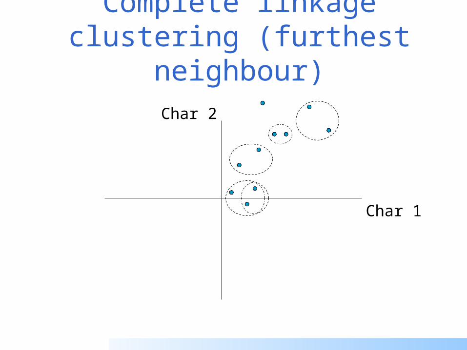
Distance from point to cluster is defined as the largest distance between that point and any point in the cluster

Complete linkage clustering (furthest neighbour)

More ‘structured’ clusters than with single linkage clustering

Let Ci and Cj be two disjoint clusters:

di,j = Max(dp,q), where p Ci and q Cj

Clustering algorithm

1. Initialise (dis)similarity matrix2. Take two points with smallest distance

as first cluster 3. Merge corresponding rows/columns in

(dis)similarity matrix4. Repeat steps 2. and 3.

using appropriate clustermeasure until last two clusters are merged

Average linkage clustering (Unweighted Pair Group Mean Averaging -UPGMA)

Char 1

Char 2

Distance from cluster to cluster is defined as the average distance over all within-cluster distances

UPGMA

Let Ci and Cj be two disjoint clusters:

1di,j = ———————— pq dp,q, where p Ci and q Cj

|Ci| × |Cj|

In words: calculate the average over all pairwise inter-cluster distances

Ci Cj

Multivariate statistics – Cluster analysis

Phylogenetic tree

Scores

Similaritymatrix

5×5

12345

C1 C2 C3 C4 C5 C6 ..

Data table

Similarity criterion

Cluster criterion

Multivariate statistics – Cluster analysis

Scores

5×5

12345

C1 C2 C3 C4 C5 C6

Similarity criterion

Cluster criterion

Scores

6×6

Cluster criterion

Make two-way ordered

table using dendrograms

Multivariate statistics – Two-way cluster analysis

14253

C4 C3 C6 C1 C2 C5

Make two-way (rows, columns) ordered table using dendrograms; This shows ‘blocks’ of numbers that are similar

Multivariate statistics – Two-way cluster analysis

Graph theory

The river Pregal in Königsberg – the Königsberg bridge problem and Euler’s graph

Can you start at some land area (S1, S2, I1, I2) and walk each bridge exactly once returning to the starting land area?

Graphs - definition

Digraphs: Directed graphs

Complete graphs: have all possible edges

Planar graphs: can be presented in 2D and have no crossing edges (e.g. chip design)

0 1 1.5 2 5 6 7 9

1 0 2 1 6.5 6 8 8

1.5 2 0 1 4 4 6 5.5

.

.

.

Graph Adjacency matrix

Graphs - definition

An undirected graph has a symmetric adjacency matrix

A digraph typically has a non-symmetric adjacency matrix

Example application – OBSTRUCT: creating

non-redundant datasets of protein structures Based on all-against-all global sequence alignment Create all-against-all sequence similarity matrix Filter matrix based on desired similarity range

(convert to ‘0’ and ‘1’ values) Form maximal clique (largest complete subgraph) by

ordering rows and columns This is an NP-complete problem (NP = non-

polynomial) and thus problem scales exponentially with number of vertices (proteins)

Example application 1 – OBSTRUCT: creating non-redundant datasets of protein

structures • Statistical research on protein structures typically

requires a database of a maximum number of non-redundant (i.e. non-homologous) structures

• Often, two structures that have a sequence identity of less than 25% are taken as non-redundant

• Given an initial set of N structures (with corresponding sequences) and all-against-all pair-wise alignments:

• Find the largest possible subset where each sequence has <25% sequence identity with any other sequence

Heringa, J., Sommerfeldt, H., Higgins, D., and Argos, P. (1992). Obstruct: a program to obtain largest cliques from a protein sequence set according to structural resolution and sequence similarity. Comp. Appl. Biosci. (CABIOS) 8, 599-600.

Example application 1 – OBSTRUCT: creating non-redundant datasets of protein

structures (Cnt.)• The problem now can be formalised as follows:

• Make a graph containing all sequences as vertices (nodes)

• Connect two nodes with an edge if their sequence identity < 25%

• Make an adjacency matrix following the above rules

Heringa, J., Sommerfeldt, H., Higgins, D., and Argos, P. (1992). Obstruct: a program to obtain largest cliques from a protein sequence set according to structural resolution and sequence similarity. Comp. Appl. Biosci. (CABIOS) 8, 599-600.

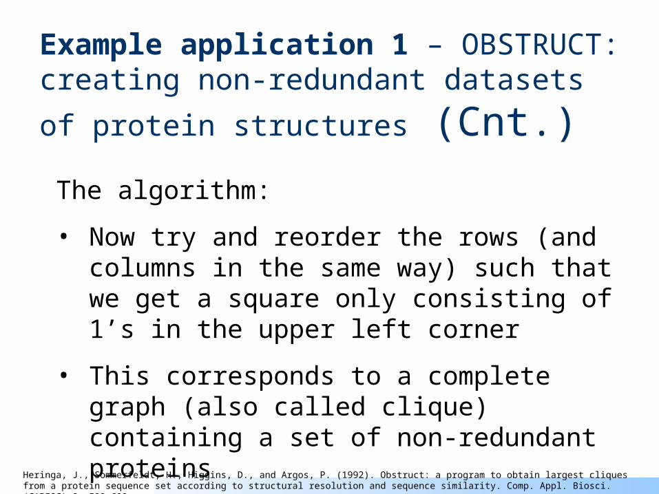
Example application 1 – OBSTRUCT: creating non-redundant datasets of protein

structures (Cnt.)

The algorithm:

• Now try and reorder the rows (and columns in the same way) such that we get a square only consisting of 1’s in the upper left corner

• This corresponds to a complete graph (also called clique) containing a set of non-redundant proteins

Heringa, J., Sommerfeldt, H., Higgins, D., and Argos, P. (1992). Obstruct: a program to obtain largest cliques from a protein sequence set according to structural resolution and sequence similarity. Comp. Appl. Biosci. (CABIOS) 8, 599-600.

Example application 1 – OBSTRUCT: creating non-redundant datasets of protein

structures (Cnt.)

1 0 1 1 1 0 0 0 1

0 1 0 0 1 1 1 0 0

1 0 1 1 1 0 1 1 0

1 0 1 1 0 0 0 0 1

. . . . . . .

5

4

6

4

..

Adjacency matrix

1. Order sum array and reorder rows and columns accordingly…

2. Estimate largest possible clique and take subset of adj. matrix containing only rows with enough 1s

3. For a clique of size N, a subset of M rows (and columns), where M N, with at least N 1s is selected.

4. Go to step 1.

Heringa, J., Sommerfeldt, H., Higgins, D., and Argos, P. (1992). Obstruct: a program to obtain largest cliques from a protein sequence set according to structural resolution and sequence similarity. Comp. Appl. Biosci. (CABIOS) 8, 599-600.

Some books call graphs containing multiple edges or loops a multigraph, and those without a graph. Other books allow multiple edges or loops in a graph, but then talk about a graph without multiple edges and loops as a simple graph.

Remarks

A multigraph might have no multiple edges or loops. Every (simple) graph is a multigraph, but not every multigraph is a (simple) graph.

Every graph is finite

Sometimes even “multigraph” folks talk about a “simple graph” to emphasize that there are no multiple edges and loops.

Further definitions

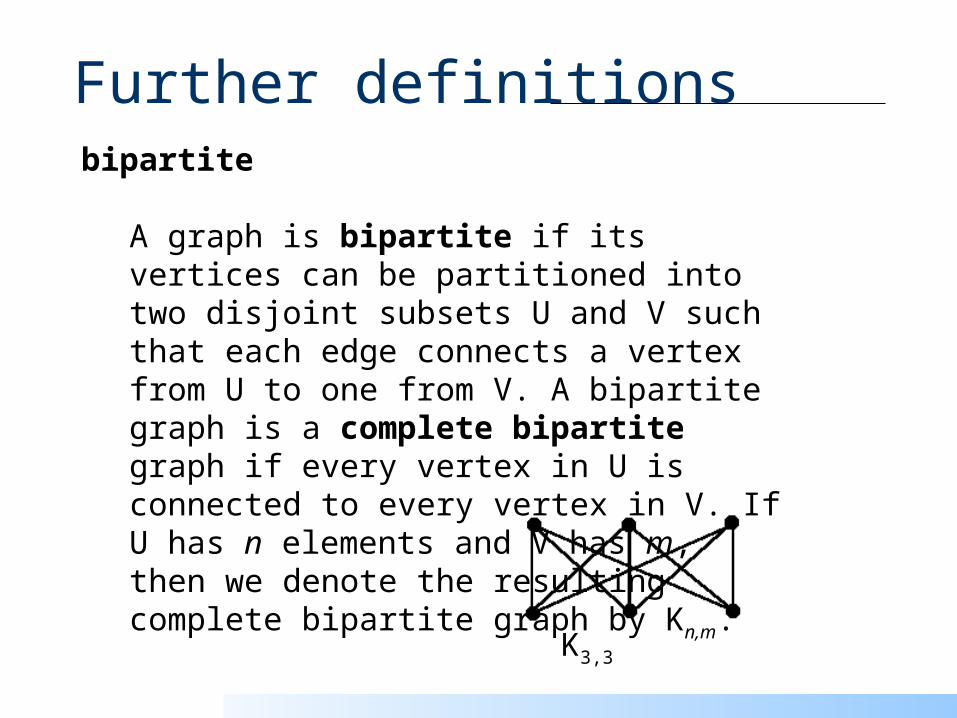
K3,3

Further definitions

K3,3

bipartite                               A graph is bipartite if its vertices can be partitioned into two disjoint subsets U and V such that each edge connects a vertex from U to one from V. A bipartite graph is a complete bipartite graph if every vertex in U is connected to every vertex in V. If U has n elements and V has m, then we denote the resulting complete bipartite graph by Kn,m.

The Stable Marriage Algorithm In mathematics, the stable marriage problem (SMP) is the

problem of finding a stable matching — a matching in which no element of the first matched set prefers an element of the second matched set that also prefers the first element.

It is commonly stated as:– Given n men and n women, where each person has ranked all

members of the opposite sex with a unique number between 1 and n in order of preference, marry the men and women off such that there are no two people of opposite sex who would both rather have each other than their current partners. If there are no such people, all the marriages are "stable".

In 1962, David Gale and Lloyd Shapley proved that, for any equal number of men and women, it is always possible to solve the SMP and make all marriages stable.

The Stable Marriage Algorithm Also called the Gale-Shapley algorithm (see preceding slide) Given two non-overlapping equally sized graphs of men (A, B,

C, ..) and women (a, b, c, …), where each man and woman has a preference list about persons of the opposite sex

A pairing denotes a 1-to-1 correspondence between men and women (each man marries one woman)

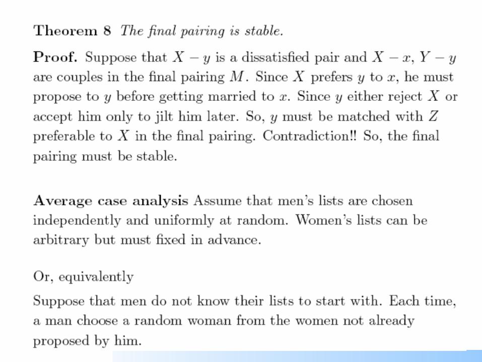
A pairing is unstable if there are couples X-x and Y-y such that X prefers y to x and y prefers X to Y– if this happens, pair X-y is called unsatisfied

A pairing in which there are no unsatisfied couples is called a stable pairing or stable marriage

The Stable Marriage Algorithm forms a bipartite graph that is stable

A: abcd denotes the preferences of A (likes a the most, then b, then c, while d is liked least)

The Stable Marriage Algorithm The Gale-Shapley pairing, in the form presented here, is male-

optimal and female-pessimal (it would be the reverse, of course, if the roles of "male" and "female" participants in the algorithm were interchanged).

To see this, consider the definition of a feasible marriage. We say that the marriage between man A and woman B is feasible if there exists a stable pairing in which A and B are married. When we say a pairing is male-optimal, we mean that every man is paired with his highest ranked feasible partner. Similarly, a female-pessimal pairing is one in which each female is paired with her lowest ranked feasible partner.

Thuis means that men pair with women higher in their preference list than where these men appear in the list of the women paired to them (on average)

0 1 1.5 2 5 6 7 9

1 0 2 1 6.5 6 8 8

1.5 2 0 1 4 4 6 5.5

.

.

.

Graph Adjacency matrix

Graphs - definition

An undirected graph has a symmetric adjacency matrix

A digraph typically has a non-symmetric adjacency matrix

A Theoretical Framework Representation of a set of n-dimensional (n-D) points as a

graph– each data point represented as a node – each pair of points represented as an edge with a weight defined by the

“distance” between the two points

0 1 1.5 2 5 6 7 9

1 0 2 1 6.5 6 8 8

1.5 2 0 1 4 4 6 5.5

.

.

.

n-D data pointsgraph

representationdistance matrix

A Theoretical Framework

Spanning tree: a sub-graph that has all nodes connected and has no cycles

Minimum spanning tree: a spanning tree with the minimum total distance

(a) (b) (c)

Spanning tree Prim’s algorithm (graph, tree)

– step 1: select an arbitrary node as the current tree – step 2: find an external node that is closest to the tree, and add it with its

corresponding edge into tree– step 3: continue steps 1 and 2 till all nodes are connected in tree.

4

10

6

7

35

8

(e)

4

7

35

(b)

4 4

(c)

7

4

3

(d)

7

(a)

Kruskal’s algorithm– step 1: consider edges in non-decreasing order – step 2: if edge selected does not form cycle, then add it into tree; otherwise

reject– step 3: continue steps 1 and 2 till all nodes are connected in tree.

(f)

4

7

35

4

10

6

7

35

8

(a) (b)

3

4

(c)

3

Spanning tree

4

3

(d)

5

4

3

(e)

5

6

reject

4

3

(e)

5

6

4

3

(e)

5

6

A Theoretical Framework A formal definition of a cluster:

– C forms a cluster in D only if for any partition C = C1 U C2, the closest point, from D-C1, to C1 is from C2, in other words, the closest connection from the points outside C1 must come from within C2

Key results

c1

c2

For any data set D, any of its cluster is represented by a sub-tree of its MST

A Theoretical Framework We can use the result on the preceding slide for

clustering using PRIM’s algorithm– The order of nodes as selected by PRIM’s algorithm defines a

linear representation, L(D), of a data set D

– We can plot the node distances in PRIM’s minimum spanning tree against the order of the nodes as they were added by PRIM’s algorithm (see earlier slide)

Any contiguous block in L(D) represents a cluster if and only if its elements form a sub-tree of the MST, plus

some minor additional conditions (each cluster forms a valley)

A B E D C

4

10

6

7

35

8

4

7

35

A AB B

C CD D

E E

edge

wei

ght

(dis

tan

ce)

PRIM’s

A Theoretical Framework

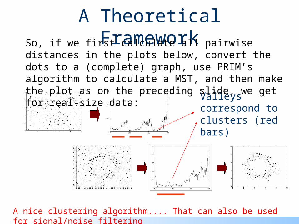
Valleys correspond to clusters (red bars)

So, if we first calculate all pairwise distances in the plots below, convert the dots to a (complete) graph, use PRIM’s algorithm to calculate a MST, and then make the plot as on the preceding slide, we get for real-size data:

A nice clustering algorithm.... That can also be used for signal/noise filtering

Take home messages Revise agglomerative clustering (e.g.

nearest/furthest neighbour, group averaging) Learn about graphs (complete, (un)directed,

adjacency matrix, bipartite, etc.) Understand the relationship between a graph and

its adjacency matrix Understand the Stable Marriage Algorithm Understand Prim’s and Kruskal’s algorithm

– Make sure you understand the clustering method based on the minimal spanning tree made by Prim’s algorithm (preceding slide)