introduction to cube - cati.org.plcati.org.pl/download/warsztaty/cube/cube-intro.pdf · cube...

of 32

INTRODUCTION TO CUBE

1 WELCOME TO CUBE...................................................................................................................... 2

1.1 OVERVIEW ................................................................................................................................... 2 1.2 THE ARCHITECTURE OF CUBE ...................................................................................................... 3 1.3 THE CUBE USER ENVIRONMENT .................................................................................................. 5 1.4 INTEGRATION WITH ARCGIS........................................................................................................ 7 1.5 INTEGRATION OF THE CUBE EXTENSIONS..................................................................................... 7

2 ABOUT THIS TUTORIAL................................................................................................................ 8

3 FORECASTING PERSONAL TRAVEL WITH CUBE................................................................. 9

3.1 GETTING STARTED WITH CUBE .................................................................................................... 9 3.2 DEVELOPING THE SCENARIO ...................................................................................................... 12

4 STUDYING A PROPOSED ROADWAY IMPROVEMENT ...................................................... 23

4.1 DEVELOPING THE SCENARIO ...................................................................................................... 24 4.2 RUNNING THE MODEL FOR THE SCENARIO ................................................................................. 24

of 32

1 Welcome to Cube

1.1 Overview

The transportation system touches almost every element of our daily lives, from how we

go to work, how our children go to school, how we move goods from place to place and

how we communicate in general. This system is intimately tied to land use, the

environment and to the economy.

The planning of the transportation system requires vision, intelligence, political savvy

and sound estimates of future travel demand. Cube is designed to accurately estimate

future travel demand and the impacts of alternative transportation policies and

improvements. Cube and its modules are used in more urban areas in the world than any

other system: from planning some of the great cities of the world (Washington, San

Francisco, Los Angeles, Hong Kong, Bangkok, Paris, and London), to helping others

prepare for the Olympics (Sydney, Atlanta, and Norway), to improving the quality of life

in many others. Cube provides robust methodologies, intelligent graphics and accurate

information within a user-friendly modern software platform.

Cube’s broad range of capabilities provides answers to all of your planning questions

from testing new public transit alternatives to road pricing strategies to new

developments to new freight terminals.

With Cube, you can generate decision-making information quickly using powerful

modeling and GIS techniques, statistics and comparisons, high quality graphical output,

and a variety of reporting methods. Cube empowers you to make smarter decisions more

quickly by uncovering key indicators for evaluating your planning alternatives. Cube is a

modular, tightly integrated, full featured product line for the transportation planning

process, covering passenger demand, freight demand, micro-simulation, air quality and

reporting.

Key features of Cube:

� Cube provides two explicit working environments:

1) The developer environment providing advanced methods and techniques

for the design and development of transport models.

2) The application environment for quick and easy application of the models

to build, test and evaluate scenarios.

� Cube has a series of Cube Extensions working within one integrated software

environment using one data source. These extensions provide capabilities for:

of 32

Passenger forecasting

Freight forecasting

Traffic micro-simulation

Trip matrix optimization

� Cube has an intuitive model design and model application workspace with

extremely easy to use data manipulation features.

� Cube provides direct access to and from ArcGIS, the industry standard for GIS

systems.

� Cube has tools for the development and sharing of high quality 2D and 3D

animations.

1.2 The Architecture of Cube

Cube is a modular system comprised of a main component, Cube Base, and Cube

Extensions which may be acquired for undertaking one or more specialized transportation

techniques.

Cube Base

Cube Base provides tools for 1) development, editing, manipulation, mapping and

graphing of data using geographic information system (GIS) techniques and other

functions, 2) design and application of the modeling and micro-simulation process,

and 3) creation, management, comparison and analysis of scenarios.

Cube Base also provides for the direct use of ArcGIS from ESRI providing

compatibility with ESRI data standards as well as the use of advanced GIS functions.

In addition to serving as the user interface for all of the Cube Extensions, Cube Base

may also be used to update and apply models developed in Citilabs’ other travel

forecasting systems, TP+, TRIPS and TRANPLAN.

Cube Extensions

1. Cube Voyager: Forecasting Personal Travel Demand

Cube Voyager combines the latest in Citilabs' technologies for the forecasting of

personal travel. Cube Voyager uses a modular and script-based structure allowing the

incorporation of any model methodology ranging from standard four-step models, to

discrete choice to activity-based approaches. Advanced methodologies provide

junction-based capacity restraint for highway analysis and discrete choice multi-route

transit path building and assignment. Cube Voyager includes highly flexible network

of 32

and matrix calculators for the calculation of travel demand and for the detailed

comparison of scenarios.

Cube Voyager was designed to provide an open and user-friendly framework for

modeling a wide variety of planning policies and improvements at the urban, regional

and long-distance level. Cube Voyager brings together these criteria within a

comprehensive library of planning functions applied under the general Cube

framework. This makes the management of data a snap, and the coding of complex

methodologies simple via a step-by-step approach.

2. Cube Cargo – Forecasting Commodity Demand and Truck Flows

Cube Cargo is used to test a wide variety of policies and infrastructure improvements,

from pricing strategies to freight-specific facilities. Cube Cargo is the Cube Extension

for freight forecasting, offering specific methodologies for studying freight demand

using a commodity-based approach. Cube Cargo operates seamlessly with all of Cube

including Cube Voyager and Cube ME. Cube Cargo also works with TP+ and TRIPS.

With Cube Cargo you can add freight forecasting by leveraging your existing

passenger data and models.

Cube Cargo forecasts:

� Matrices of tons of goods by commodity type by mode for use in the analysis of

goods flows, and

� Matrices of the number of trucks by truck type ready to be assigned to estimate

truck vehicle flows.

3. Cube Dynasim – Multimodal Traffic Microsimulation

Cube Dynasim is a powerful software system that helps the planner and engineer to

design and analyze the interaction between alternative infrastructure, operating

characteristics and travel demand. Cube Dynasim enables the user to simulate any

size system in a user-friendly graphical environment. Data are easily shared with

other Cube functional libraries.

Cube Dynasim captures the full dynamics of time dependent traffic phenomena using

sophisticated driver behavior models. Cube Dynasim performs detailed operational

analysis of complex traffic on roadways while realistically emulating the flow of

automobiles, trucks, buses, rail and pedestrians.

Cube Dynasim provides stunning 2D and 3D animations and graphics for clear

evaluation.

4. Cube ME – statistically optimized trip matrix estimation

of 32

One of the most valuable pieces of data in transportation planning is an accurate

origin-destination matrix of existing travel. It is the basis for forecasting and for

almost all important comparative analyses. Cube ME is the Cube Extension

developed specifically for estimating and updating base year automobile, truck and

public transit trip matrices. Cube ME enables the user to exploit a wide variety of data

that contribute to matrix updating and matrix development. Cube ME uses

mathematical techniques to find trip matrices that are consistent with observed

transport demand and count data. It does what many do by hand, but in a much more

accurate and efficient way.

1.3 The Cube User Environment

The user environment of Cube has 3 principal windows:

� Graphics: for network development, editing and high quality charting and

mapping

� Application Manager: the flow chart interface for building and documenting the

model process

� Scenario Manager: the left-hand column used for managing scenario and

associated input and output data and reports.

Cube Base - The User Interface of Cube

of 32

Cube has two specific modes of operation known as:

Developer Mode, and

Appliers Mode

When Cube is operating in Developer Mode, the environment is set for designing a

model structure, manipulating the associated data and for creating all of the interfaces for

efficient use of the model system. The primary interface in Developer Mode is the flow-

chart style Application Manager.

Cube in Developer Mode

By selecting Appliers Mode, much of the model system itself including the model steps,

model coefficients and other parameters are put in read-only mode. The primary interface

in Appliers Mode is Scenario Manager and its associated model menu screen. The model

menu can be customized in any way to make the use of the model system very easy to use,

eliminating the need for experts in travel modeling when developing and testing scenarios.

of 32

Cube in Applier Mode

1.4 Integration with ArcGIS

In addition to the three principal Cube windows, Cube provides direct access to ArcGIS

from ESRI. Moving data to ArcGIS is facilitated by switching from Cube Graphics to

ArcGIS via the clicking of the ArcGIS icon located at the bottom right of the Cube

interface.

All of the layers and all of their data are transferred to ArcGIS along with a standard

ArcGIS *.mxd file. These data are put within ArcGIS in ESRI standard shape format.

The analyst can then use the data within ArcGIS and easily bring this data back to Cube

for modeling and simulation.

1.5 Integration of the Cube Extensions

The Cube Extensions, Cube Voyager, Cargo, Dynasim and ME, are addressed through

the Application Manager window. Other products from Citilabs, such as TRIPS, TP+ and

TRANPLAN may also be integrated in this way.

of 32

This programs or functions are then used within Application Manager as the functions to

be used in developing a modeling and simulation process. Other User Programs

(specialized routines in C++, C, Fortran or any other programming language) can be

easily incorporated in this way. Equally, third party software products such as Microsoft

Excel and Crystal Reports from Crystal Decisions may be integrated within the

Cube working environment.

2 About This Tutorial

This tutorial was developed to help you to understand and to learn how to use Cube. It is

not intended to be a comprehensive users guide or to replace training courses, but is

intended to help you understand how Cube works, what Cube can do and how to start

using Cube in your transportation analysis.

This tutorial takes you through a series of interactive exercises to discover the

functionalities provided by Cube. The tutorial concludes with a discussion of services

offered by Citilabs to help you migrate your existing model or to develop a new model

system, our training courses our user support and our user forum.

You will be provided with a website that contains Cube and data to be used in the lessons

contained in this guide. You should run the installation Cube prior to starting the lessons

outlined below. When you install the Cube Software and Data, just click the Cube

setup.exe in your system. A startup menu should appear.

of 32

Select “install demonstration version” to install the demonstration version of Cube and

follow the instructions on the screen.

3 Forecasting Personal Travel with Cube

We take you through a project that shows how you would apply a typical travel-

forecasting model in a real situation. The project uses a forecasting model and datasets

included on the Cube web site (provided later) or in the lab. If you have not yet installed

the software and datasets, please refer to Chapter 2.

One of the most common uses of a travel forecasting system is to estimate the traffic

generated to and from a new housing, commercial or office development. In this example,

we will use the Cube Demonstration Model to estimate the consequences of a new

development on travel flow.

3.1 Getting Started with Cube

The steps to start this Cube project are as follows:

Step 1: Start Cube by double-clicking the Cube icon on your computer desktop.

(Alternatively, click the Start button on the Windows taskbar, point to

Programs, point to Citilabs, click Cube.)

Step 2: When Cube opens, you see the Cube start-up dialog on top of the application

window.

Step 3: In the Cube dialog, click the option to Demo Data.

of 32

This will open a Cube Catalog. A catalog holds all of the models, data and scenarios.

In the Cube dialog, click the option to Demo Data. The demonstration catalog is shown

with 3 sub-windows:

Scenarios: These are where we will develop our scenario and apply the model.

Data: It holds the input and output data for each of the scenarios. This provides

quick access to these files.

Applications: These are the available model processes that we can apply. In this section,

we will be using the Cube Demonstration Model.

Prior to setting up the scenario for our new development, let’s get familiar with the model

that will be used to test this new development.

Step 4: Double click on Cube Voyager Demonstration Model.app in the Applications

sub-window. The model should open shown below.

Data

Scenarios

Applications

of 32

This window of Cube is known as Application Manager. It is a flow-chart

view of the model process. Cube is operating in what is called ‘Appliers

Mode’. This has taken the model and put it in a form that is easy to use by

those who develop and run scenarios. In this mode, you cannot change the

model, but you may apply the model. Later chapters in this tutorial take you

through exercises in developing model structures where you can learn how to

design and calibrate the model.

This model is a ‘4-step’ model of Trip Generation, Trip Distribution, Mode

Choice and Assignment. It has other ‘steps’ for developing networks and for

doing various analyses of the results.

Cube is very open and flexible. Model developers are provided the tools to

build almost any structure that might be desired including emerging methods

in activity models and tour-based approaches. We have used a 4-step model in

the demonstration system as it is the most commonly used structure in most

locations in the world.

The flow chart shows the steps in the model. Each of these steps shows light

blue boxes on the left-hand side and green boxes on the right-hand side. The

light blue boxes are inputs to the step and the green are the outputs of the steps.

Linkages are made taking outputs to serve as inputs, etc.

This model also includes a ‘loop’ and a ‘branch’. In this model, a loop has

been placed around the distribution, mode choice and assignment stages of the

model. This is what is known as a ‘feedback loop’ taking the travel times from

the assignment model (congested travel time) and bringing that back to

distribution to distribute the trips from zone to zone using these congested

of 32

times. These are also used in the mode choice stage. The model iterates

between these steps until a criteria has been achieved.

The branch is used to select whether detailed analyses are requested or not.

3.2 Developing the Scenario

In this Cube project we will apply the model to see the impacts associated with a new

shopping center planned for our study town, Cubetown.

The model already has a ‘base case’ setup. It is located in the Scenarios sub-window and

called Base.

Double-click on ‘Base’ in the scenario sub-window. The interface for applying the model

opens as shown below.

This interface, along with the questions, the colors and logo, has been designed by the

developer of the model using ‘developer mode’ in Cube. A model interface can have any

questions that you would like to ask, any colors and any logos or other images. This

allows you to build a customized interface for your model.

of 32

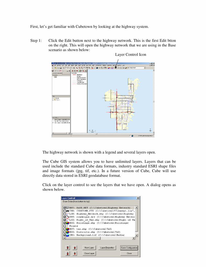
First, let’s get familiar with Cubetown by looking at the highway system.

Step 1: Click the Edit button next to the highway network. This is the first Edit btton

on the right. This will open the highway network that we are using in the Base

scenario as shown below:

Layer Control Icon

The highway network is shown with a legend and several layers open.

The Cube GIS system allows you to have unlimited layers. Layers that can be

used include the standard Cube data formats, industry standard ESRI shape files

and image formats (jpg, tif, etc.). In a future version of Cube, Cube will use

directly data stored in ESRI geodatabase format.

Click on the layer control to see the layers that we have open. A dialog opens as

shown below.

of 32

We have a highway network open and active, a public transit layer open but not shown

on the screen and various shape and image layers. A drawing layer is also open. This

layer is where you can place road signs and other information on the map.

Click on the check mark next to the TRN layer

Click Save Configuration

Click Close

The map is now re-drawn with the transit layer shown.

Now, let’s zoom to the area that will hold our shopping center.

Click View

Click Restore

Select Shopping Center

of 32

You will see the following display:

This moves the map to the area where the shopping center will be located. We had

previously bookmarked this zoom. You can bookmark up to 16 views and save this in the

GIS workspace.

of 32

Our shopping center will be located as shown in the image above.

It will have access to the roadway and transit line running in front. We also have a major

road located not far away, route 81.

3.2.1 Running the Model for the Base Case

Close the map window by clicking on the small ‘x’ in the upper right-hand corner. Save

the project file when prompted. You should now see our scenario window.

The base scenario has previously been prepared. Run the scenario by clicking on run at

the bottom of the menu.

The ‘task monitor’ window appears and shows the progress of the model run.

When the model has finished, a dialog box will appear. Click OK.

Let’s look at the traffic assigned to our shopping center area, prior to implementing the

shopping center.

Move your mouse to the Data sub-window in the column. Click on the ‘+’ on the

Outputs.

Click on ‘+’ next to Highway Assignment

Double-click the HW Intersections file.

of 32

This opens the assigned network and estimated intersection flows for the tested scenario

(see Picture below)

The map has opened to the previously zoomed area (if not select View, Restore,

Shopping Center).

Turn off the transit layer by selecting the layer control.

Uncheck the box next to TRN.

Click Save Configuration.

Click Close.

Click on the pull-down arrow on the node color icon (see Below).

of 32

Click on Level of Service

Click on the pull-down arrow on the link color icon

Click on V/C ratios

We can now see the current traffic conditions around the shopping center. The

intersections and roadways are at a good quality of level of service.

Close the map window by clicking on the small ‘x’ in the upper right hand corner.

When prompted to save the project file select Yes. This saves the selected node and color

settings and location.

of 32

3.2.2 Running the Model for the Scenario

Let’s add in the shopping center and create a new scenario.

Right-click on ‘Base’ in the scenario sub-window.

Select Add Child

Type in: Future Year

When the description dialog appears, click OK.

You could add notes here about the scenario.

Right-click on Future Year

Select Add Child

Type in: Citimart

When the description appears, click OK.

The user menu now opens and is using, by default, all of the values from the Base

scenario. We will make one change: adding in the proposed shopping center in the

demographic data.

Click on edit next to the demographic data (TAZ).

When prompted to make a copy of the file, Click Yes and name the file “tazfuture.dbf”.

Also click Yes when the below window is prompted.

Cube has made a copy and opened the new file.

Our shopping center will add 1500 retail jobs. Replace the existing values in total jobs

and retail jobs as follows:

Type in: 2885 for total jobs and 1557 for retail jobs for zone 1

of 32

After making the changes click on a different row so that you exit edit mode before

closing the file by clicking on the small ‘x’. The file will automatically be saved. Note:

there is currently no undo feature when editing DBF files.

Click the Run button

This will now apply the model for the new scenario. A dialog will appear when the model

run has completed. Close that dialog.

Now, let’s look at the assignment results.

Make sure that the scenario Citimart is highlighted in the scenarios sub-window.

Double-click on HW intersections in the Data window.

The map opens in the same zoom as before with the same color sets selected except now

we see the results from the Citimart scenario. The level of service and volume/capacity

ratio has changed with the new Citimart.

Cube can be used to obtain an enormous variety of results and tables. Not all are shown

here in this document. We have seen the volume and capacity and intersection level of

service with and without the Citimart. It may also be useful to see the location and

volume of travelers coming to and from the Citimart. This will show us the roadways that

are being impacted by the development.

Click on Path, Click on Use Path File

Navigate to c:\cubetown\model\base\future year\citimart

Select roadpaths.pth as shown below.

Click Open

of 32

An information box appears with a summary of the information contained within this file.

Click OK. A new menu is added

Pull-down on the Mode menu

Select Selected Zones

You can either click on the zone centroid for zone 1 or just type in 1 for the origin.

For the destination, enter 2-25

Check Post Volumes

Check Single Color and select Red

Click Display. The volumes coming from Citimart are displayed as shown below. It

shows the routes that they use as well. A bandwidth is displayed of the level of traffic and

the actual value is posted.

of 32

Zoom to the shopping Center as shown below:

You will see the flow as shown below:

of 32

4 Studying a Proposed Roadway Improvement

We will build on the work done in Chapter 3. In Chapter 3, we applied the model for our

base situation and then created a new scenario with our shopping center, Citimart. We

saw that the creation of Citimart leads to increased and unacceptable levels of traffic on

the roadways and intersections nearby. We also saw the routes of travelers from the new

shopping center.

We will make, in this chapter, some improvements to the roadway and intersections

nearby and test the impact of these improvements.

If Cube is not open: (otherwise, advance to Developing the Scenario)

Start Cube by double-clicking the Cube icon on your computer desktop.

(Alternatively, click the Start button on the Windows taskbar, point to Programs,

point to Citilabs, click Cube.)

When Cube opens, you see the Cube start-up dialog on top of the application window.

In the Cube dialog, click the option to Demo Data.

Open Discover Cube.cat as shown in the following graphic, and click Open.

Double click on Cube Voyager Demonstration Model.app in the Applications

sub-window. The model should open in the main window.

of 32

4.1 Developing the Scenario

In this section we will apply the model to see the impacts associated with a new shopping

center planned for our study town, Cubetown and some improvements to the roadway

and the intersections.

4.2 Running the Model for the Scenario

Citimart has already been added to our demographic data file tazcitimart.dbf. However,

we need to modify the highway network to represent the improvements that we wish to

test. First, let’s add in the new scenario.

Right-click on ‘Citimart’ in the scenario sub-window

Select Add Child

Type in: Citimart with Road

When the description dialog appears, click OK. You could add notes here about

the scenario.

The user menu now opens and is using, by default, all of the values from the Citimart

scenario—its parent scenario. We will make one change: adding in the proposed roadway

improvements near the proposed shopping center.

Click on edit next to the highway network.

When prompted to make a copy of the file, Click Yes and name the file

“citimart.net”.

Cube has made a copy and opened the new file.

The highway network opens. Let’s look at the existing roadways.

If you are not zoomed to the Citimart area, click View, click Restore and select

Shopping Center

Pull down on the link color menu and select Number of Lanes.

of 32

This splits the links into their directions and shows the number of lanes by

direction. The roadways around the shopping center have 1 lane in each direction.

In this project, we will add a lane in each direction to the roadways in the area. First let’s

zoom out a bit. Select the zoom out cursor and click once in the center of the map. You

should have the following on your screen.

Click Polygon

Click New. This changes the cursor to a crosshair.

Click on points to create a polygon similar to that shown below. To close the

polygon, either click near the beginning or hold C and click. Your polygon should

resemble that shown in the image below.

of 32

Click Link

Click Compute

On the pull-down, select set 10

In the large white box between Name: and Applies To:, right-click.

Select Insert. This will open a space to enter a dialog

Right click in the dialog white space. This will bring a list of the attributes on

your network links.

Using Right-click or typing, type in the formula as shown below.

Click OK

of 32

On the Applies To dialog, pull down and select: All Items Inside and Crossing

Polygon NOW

On the Condition, type in FUNC_CLASS=1-6

This is saying to add 1 lane to all facilities that are within or cross the polygon.

However, only add these to links where the roadway type is 1-6 (i.e. not our

centroids connectors).

Your dialog should resemble the image shown below.

Save the network by clicking on the button

We will now modify the intersections

Select Intersection

Select Open/Create Input Intersection Data File

Navigate to: C:\cubetown\highway network. Open the file titled: base.ind.

Let’s save this to a new file.

Click Intersection

of 32

Click Save Intersection Data File As

Enter: citimart.ind and click Save

Click Post

Click Intersection Locations. You should see the following on the screen.

We will now modify one of the signalized intersections and then copy that new setting to

the others.

Make sure you are in Pointing Mode and click on intersection 788 located at the bottom

of the screen within the polygon as shown below.

The highway node information appears.

Click on the cross-hair icon on this dialog. We will modify the lane geometry at

this intersection.

Click on Lane Geometry

of 32

Modify the diagram until you have as shown below.

Add a right-turn-only lane in the southbound direction with 2 straight only lanes,

a second straight-only lane in the northbound direction, and add a left-turn-only

lane in the eastbound direction. When completed, Click Save. Then, Click Save to

Library. Click Browse and select Citilabs.ilb. Click Open.

In the Intersection Name dialog, type: Cubetown and Click OK. Click OK on the

Information Dialog. Click OK to exit.

Open each of the intersections within the polygon and add a lane to the turning

movements. For the intersection that currently has a stop sign, Select Copy from

Library. Select Cubetown.

Go to the Lane Geometry and update to be as shown below:

of 32

Click Save, Click OK

After you have adjusted all of the intersections within the polygon, close the

dialog and Click Intersection

Click Save Intersection Data File

Overwrite the existing file if prompted

Click Polygon, Click Hide

Click the refresh icon

You should now have signals at each of the intersections. Your screen should

appear as below.

Close the map. If prompted save, save the project file.

of 32

You should now be back in the user menu. If not, double click on the Citimart

with Road in the Scenario sub-window.

Update the information on the screen for Citimart with Road to use the new

Intersection file (citimart.ind) and the new highway network (citimart.net). When

completed your screen should appear as below.

Click Save

Click Run. The scenario will be tested. When it finishes a dialog will appear.

Click OK.

This will now apply the model for the new scenario. A dialog will appear when

the model run has completed. Close that dialog.

Now, let’s look at the assignment results. Make sure that the scenario Citimart

with Road is highlighted in the scenarios sub-window.

Double-click on HW intersections in the Data window.

The map opens in the same zoom as before with the same color sets selected

except now we see the results from the Citimart scenario. Pull down from the link

color icon and select the VC ratio for the links. The level of service and

volume/capacity ratio has changed with the new Citimart and Road

Improvements. Some intersections continue to have level of service problems and

in a real study, further improvements might be considered and tested.

of 32

Close the map by clicking on the small ‘x’ in the upper right hand corner. When

prompted, Save the project file. Click Close on the model menu.

introduction to cube - cati.org.plcati.org.pl/download/warsztaty/cube/cube-intro.pdf · cube...

Documents