Intro to the lifecontingencies R package

Giorgio Alfredo Spedicato, Ph.D C.Stat ACAS

19th April 2015

Intro

I The lifecontingencies package (Spedicato 2013) will beintroduced.

I As first half 2015 it is the first R (Team 2012) packagemerging demographic and financial mathematics function inorder to perform actuarial evaluation of life contingentinsurances (annuities, life insurances, endowments, etc).

I The applied examples will shown: how to load the R package,how to perform basic financial mathematics and demographiccalculations, how to price and reserve financial products.

Intro

I The lifecontingencies package (Spedicato 2013) will beintroduced.

I As first half 2015 it is the first R (Team 2012) packagemerging demographic and financial mathematics function inorder to perform actuarial evaluation of life contingentinsurances (annuities, life insurances, endowments, etc).

I The applied examples will shown: how to load the R package,how to perform basic financial mathematics and demographiccalculations, how to price and reserve financial products.

Intro

I The lifecontingencies package (Spedicato 2013) will beintroduced.

I As first half 2015 it is the first R (Team 2012) packagemerging demographic and financial mathematics function inorder to perform actuarial evaluation of life contingentinsurances (annuities, life insurances, endowments, etc).

I The applied examples will shown: how to load the R package,how to perform basic financial mathematics and demographiccalculations, how to price and reserve financial products.

I The final example will show how to mix lifecontingencies anddemography (Rob J Hyndman et al. 2011) function to assessthe mortality development impact on annuities.

I The interested readers are suggested to look to the package’svignettes (also appeared in the Journal of Statistical Sofware)for a broader overview. (Dickson, Hardy, and Waters 2009; andMazzoleni 2000) provide and introduction of ActuarialMathematics theory.

I Also (Charpentier 2012) and (Charpentier 2014) discuss thesoftware.

I The final example will show how to mix lifecontingencies anddemography (Rob J Hyndman et al. 2011) function to assessthe mortality development impact on annuities.

I The interested readers are suggested to look to the package’svignettes (also appeared in the Journal of Statistical Sofware)for a broader overview. (Dickson, Hardy, and Waters 2009; andMazzoleni 2000) provide and introduction of ActuarialMathematics theory.

I Also (Charpentier 2012) and (Charpentier 2014) discuss thesoftware.

I The final example will show how to mix lifecontingencies anddemography (Rob J Hyndman et al. 2011) function to assessthe mortality development impact on annuities.

I The interested readers are suggested to look to the package’svignettes (also appeared in the Journal of Statistical Sofware)for a broader overview. (Dickson, Hardy, and Waters 2009; andMazzoleni 2000) provide and introduction of ActuarialMathematics theory.

I Also (Charpentier 2012) and (Charpentier 2014) discuss thesoftware.

First moves into the lifecontingecies package

Loading the package

I The package is loaded using

library(lifecontingencies) #load the package

I It requires a recent version of R (>=3.0) and the markovchainpackage (Spedicato 2015). The development version of thepackage requires also Rcpp package (Eddelbuettel 2013).

First moves into the lifecontingecies package

Loading the package

I The package is loaded using

library(lifecontingencies) #load the package

I It requires a recent version of R (>=3.0) and the markovchainpackage (Spedicato 2015). The development version of thepackage requires also Rcpp package (Eddelbuettel 2013).

Financial mathematics

I Actuarial mathematics calculation applies probability toquantify uncertainty on present values calculation.

I Certain present value calculations can be directly evaluated bythe package

capitals <- c(-1000,200,500,700)times <- c(0,1,2,5)#calculate a present valuepresentValue(cashFlows=capitals, timeIds=times,

interestRates=0.03)

## [1] 269.2989

Financial mathematics

I Actuarial mathematics calculation applies probability toquantify uncertainty on present values calculation.

I Certain present value calculations can be directly evaluated bythe package

capitals <- c(-1000,200,500,700)times <- c(0,1,2,5)#calculate a present valuepresentValue(cashFlows=capitals, timeIds=times,

interestRates=0.03)

## [1] 269.2989

I The presentValue function is the kernel of functions that areused to calculate annuities and accumulated values, also paidin fractional k payments.

ann1 <- annuity(i=0.03, n=5, k=1, type="immediate")ann2 <- annuity(i=0.03, n=5, k=12, type="due")c(ann1,ann2)

## [1] 4.579707 4.653791

I Such functions can be combined to price bonds and otherclassical financial products.

I The following code exemplifies the calculation of a 5% couponbond at 3% yield rate when the term is ten year.

bondPrice<-5*annuity(i=0.03,n=10)+100*1.03^-10bondPrice

## [1] 117.0604

I Such functions can be combined to price bonds and otherclassical financial products.

I The following code exemplifies the calculation of a 5% couponbond at 3% yield rate when the term is ten year.

bondPrice<-5*annuity(i=0.03,n=10)+100*1.03^-10bondPrice

## [1] 117.0604

Managing lifetables and actuarial tables

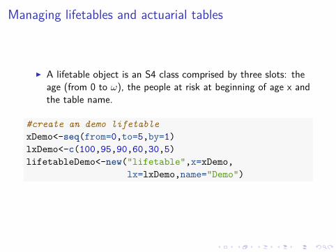
I A lifetable object is an S4 class comprised by three slots: theage (from 0 to ω), the people at risk at beginning of age x andthe table name.

#create an demo lifetablexDemo<-seq(from=0,to=5,by=1)lxDemo<-c(100,95,90,60,30,5)lifetableDemo<-new("lifetable",x=xDemo,

lx=lxDemo,name="Demo")

I In practice, it is often more convenient to load an existing tablefrom a CSV or XLS source. Some common tables have beenbundled as data.frames within the package.

I The example that follows creates the Italian IPS55 life table.

data(demoIta) #using the internal Italian LT data setlxIPS55M <- with(demoIta, IPS55M)#performing some fixingspos2Remove <- which(lxIPS55M %in% c(0,NA))lxIPS55M <-lxIPS55M[-pos2Remove]xIPS55M <-seq(0,length(lxIPS55M)-1,1)#creating the tableips55M <- new("lifetable",x=xIPS55M,lx=lxIPS55M,name="IPS 55 Males")

I In practice, it is often more convenient to load an existing tablefrom a CSV or XLS source. Some common tables have beenbundled as data.frames within the package.

I The example that follows creates the Italian IPS55 life table.

data(demoIta) #using the internal Italian LT data setlxIPS55M <- with(demoIta, IPS55M)#performing some fixingspos2Remove <- which(lxIPS55M %in% c(0,NA))lxIPS55M <-lxIPS55M[-pos2Remove]xIPS55M <-seq(0,length(lxIPS55M)-1,1)#creating the tableips55M <- new("lifetable",x=xIPS55M,lx=lxIPS55M,name="IPS 55 Males")

I It is therefore easy to perform standard demographiccalculations with the aid of package functions.

# decrements between age 65 and 70dxt(ips55M, x = 65, t = 5)

## [1] 3659.74

# probabilities of death between age 80 and 85qxt(ips55M, x = 80, t = 2)

## [1] 0.07264833

# expected curtate lifetimeexn(ips55M, x = 65)

## [1] 21.96873

Pricing and reserving Life Contingent insurances

I The pricing and reserving of pure endowments A 1x :n , term

insurances, A1x :n , annuities a{m}x , endowments A 1

x :n can beeasily handled within the package.

I Performing such actuarial calculations requires to create anactuarial table (similar to a lifetable but with one more slot forthe interest rate) that can be create as it is shown below.

#creates a new actuarial tableips55Act<-new("actuarialtable",x=ips55M@x,lx=ips55M@lx,interest=0.02,name="IPS55M")

Pricing and reserving Life Contingent insurances

I The pricing and reserving of pure endowments A 1x :n , term

insurances, A1x :n , annuities a{m}x , endowments A 1

x :n can beeasily handled within the package.

I Performing such actuarial calculations requires to create anactuarial table (similar to a lifetable but with one more slot forthe interest rate) that can be create as it is shown below.

#creates a new actuarial tableips55Act<-new("actuarialtable",x=ips55M@x,lx=ips55M@lx,interest=0.02,name="IPS55M")

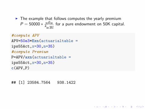
I The example that follows computes the yearly premiumP = 50000 ∗ 35E30

a30:35

for a pure endowment on 50K capital.

#compute APVAPV=50e3*Exn(actuarialtable =ips55Act,x=30,n=35)#compute PremiumP=APV/axn(actuarialtable =ips55Act,x=30,n=35)c(APV,P)

## [1] 23584.7564 938.1422

I The package allows to easily perform sensitivities on thefinancials changing key parameters like term, interest, etc as wecan see on a endowment purchased by a 30 years oldpolicyholder for 30 years.

#defining the rangesinterest.range<-seq(from=0.015, to=0.035,by=0.001)term.range<-seq(from=20, to=40,by=1)#computing APV sensitivitiesapv.interest.sensitivity<-sapply(interest.range,FUN = "AExn",actuarialtable=ips55Act,x=30,n=30)apv.term.sensitivity<-sapply(term.range,FUN = "AExn",

actuarialtable=ips55Act,x=30)

I The graph below displays sensitivities on APV varying interestrate and insurance term.

0.015 0.025 0.035

0.40

0.45

0.50

0.55

0.60

0.65

APV by Interest Rate

interest rate

AP

V

20 30 40

0.50

0.55

0.60

0.65

APV by term

term

AP

V

I Also, calculation of outstanding reserves is made easy as thefollowing example, applied on a 100K face value 40 year termterm life insurance with payments made yearly on apolicyholder aged 25, shows.

#compute the APV and premiumAPV=100e3*Axn(actuarialtable = ips55Act,x=25,n=40)P=APV/axn(actuarialtable = ips55Act,x=25,n=40)#define a reserve functionreserveFunction<-function(t)

100e3*Axn(actuarialtable = ips55Act,x=25+t,n=40-t) -P *axn(actuarialtable = ips55Act,x=25+t,n=40-t)

reserve<-sapply(0:40,reserveFunction)

0 10 20 30 40

050

010

0015

00Reserve

Policy Age

Res

erve

out

stan

ding

Stochastic evalutation

I The APV of a life contingent insurance is the expected value ofa function of a random variable (the residual life time).Knowing the interest rate and the underlying life table it ispossible both to compute the APV and to assess thedistribution of the underlying life insurance.

#analyzing and Endowment of 100K on x=40, n=25#compute APVAPV=AExn(actuarialtable = ips55Act,x=40,n=25)#samplingAEXnDistr<-rLifeContingencies(n=10e3,lifecontingency = "AExn",x = 40,t=25,object = ips55Act)

I In order to assess if the distribution is unbiased we use aclassical one sample t - test.

#assess if the expected value match the theoretical onet.test(x=AEXnDistr,mu = APV)

#### One Sample t-test#### data: AEXnDistr## t = 1.3102, df = 9999, p-value = 0.1902## alternative hypothesis: true mean is not equal to 0.6148635## 95 percent confidence interval:## 0.6146427 0.6159746## sample estimates:## mean of x## 0.6153086

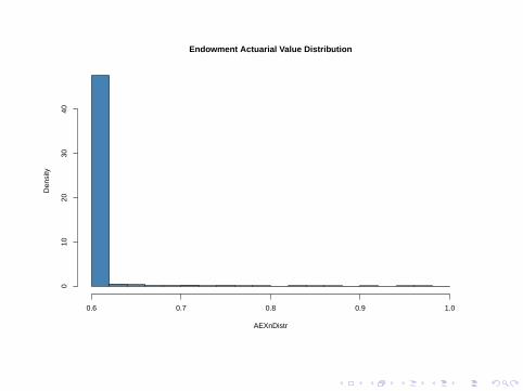
Endowment Actuarial Value Distribution

AEXnDistr

Den

sity

0.6 0.7 0.8 0.9 1.0

010

2030

40

Assessing longevity impact on annuities usinglifecontingencies and demography

I This part of the presentation will make use of the demographypackage to calibrate Lee Carter (Lee and Carter 1992) model,log (µx ,t) = ax + bx ∗ kt → px ,t = exp−µx,t ,projectingmortality and implicit life tables.

#load the package and the italian tableslibrary(demography)#italy.demo<-hmd.mx("ITA", username="yourUN",#password="yourPW")load(file="mortalityDatasets.RData") #load the dataset

I Lee Carter model is calibrated using lca function.

I Then an arima model is used to project (extrapolate) theunderlying kt over the historical period.

#calibrate lee carteritaly.leecarter<-lca(data=italyDemo,series="total",

max.age=103,adjust = "none")#perform modeling of kt serieskt.model<-auto.arima(italy.leecarter$kt)#projecting the ktkt.forecast<-forecast(kt.model,h=100)

I Lee Carter model is calibrated using lca function.I Then an arima model is used to project (extrapolate) the

underlying kt over the historical period.

#calibrate lee carteritaly.leecarter<-lca(data=italyDemo,series="total",

max.age=103,adjust = "none")#perform modeling of kt serieskt.model<-auto.arima(italy.leecarter$kt)#projecting the ktkt.forecast<-forecast(kt.model,h=100)

-The code below generates the matrix of prospective life tables

#indexing the ktkt.full<-ts(union(italy.leecarter$kt, kt.forecast$mean),

start=1872)#getting and defining the life tables matrixmortalityTable<-exp(italy.leecarter$ax+italy.leecarter$bx%*%t(kt.full))rownames(mortalityTable)<-seq(from=0, to=103)colnames(mortalityTable)<-seq(from=1872,to=1872+dim(mortalityTable)[2]-1)

historical and projected KT

year

kt

1900 1950 2000 2050 2100

−30

0−

200

−10

00

100

I now we need a function that returns the one-year deathprobabilities given a year of birth (cohort.

getCohortQx<-function(yearOfBirth){

colIndex<-which(colnames(mortalityTable)==yearOfBirth) #identify

#the column corresponding to the cohort#definex the probabilities from which#the projection is to be takenmaxLength<-min(nrow(mortalityTable)-1,

ncol(mortalityTable)-colIndex)qxOut<-numeric(maxLength+1)for(i in 0:maxLength)

qxOut[i+1]<-mortalityTable[i+1,colIndex+i]#fix: we add a fictional omega age where#death probability = 1qxOut<-c(qxOut,1)return(qxOut)

}

I Now we use such function to obtain prospective life tables andto perform actuarial calculations. For example, we cancompute the APV of an annuity on a workers’ retiring at 65assuming he were born in 1920, in 1950 and in 1980. We willuse the interest rate of 1.5% (the one used to compute ItalianSocial Security annuity factors).

I The first step is to generate the life and actuarial tables

#generate the life tablesqx1920<-getCohortQx(yearOfBirth = 1920)lt1920<-probs2lifetable(probs=qx1920,type="qx",name="Table 1920")at1920<-new("actuarialtable",x=lt1920@x,lx=lt1920@lx,interest=0.015)qx1950<-getCohortQx(yearOfBirth = 1950)lt1950<-probs2lifetable(probs=qx1950,type="qx",name="Table 1950")at1950<-new("actuarialtable",x=lt1950@x,lx=lt1950@lx,interest=0.015)qx1980<-getCohortQx(yearOfBirth = 1980)lt1980<-probs2lifetable(probs=qx1980,type="qx",name="Table 1980")at1980<-new("actuarialtable",x=lt1980@x,lx=lt1980@lx,interest=0.015)

I Now we use such function to obtain prospective life tables andto perform actuarial calculations. For example, we cancompute the APV of an annuity on a workers’ retiring at 65assuming he were born in 1920, in 1950 and in 1980. We willuse the interest rate of 1.5% (the one used to compute ItalianSocial Security annuity factors).

I The first step is to generate the life and actuarial tables

#generate the life tablesqx1920<-getCohortQx(yearOfBirth = 1920)lt1920<-probs2lifetable(probs=qx1920,type="qx",name="Table 1920")at1920<-new("actuarialtable",x=lt1920@x,lx=lt1920@lx,interest=0.015)qx1950<-getCohortQx(yearOfBirth = 1950)lt1950<-probs2lifetable(probs=qx1950,type="qx",name="Table 1950")at1950<-new("actuarialtable",x=lt1950@x,lx=lt1950@lx,interest=0.015)qx1980<-getCohortQx(yearOfBirth = 1980)lt1980<-probs2lifetable(probs=qx1980,type="qx",name="Table 1980")at1980<-new("actuarialtable",x=lt1980@x,lx=lt1980@lx,interest=0.015)

I Now we can evaluate a65 and e65 for workers born in 1920,1950 and 1980 respectively.

cat("Results for 1920 cohort","\n")

## Results for 1920 cohort

c(exn(at1920,x=65),axn(at1920,x=65))

## [1] 16.51391 15.14127

cat("Results for 1950 cohort","\n")

## Results for 1950 cohort

c(exn(at1950,x=65),axn(at1950,x=65))

## [1] 18.72669 16.83391

cat("Results for 1980 cohort","\n")

## Results for 1980 cohort

c(exn(at1980,x=65),axn(at1980,x=65))

## [1] 20.47112 18.13948

Bibliography I

Charpentier, Arthur. 2012. “Actuarial Science with R 2: LifeInsurance and Mortality Tables.”http://freakonometrics.blog.free.fr/index.php?post/2012/04/04/Life-insurance,-with-R,-Meielisalp.

———. 2014. Computational Actuarial Science. The R Series.Cambridge University Press.

Dickson, D.C.M., M.R. Hardy, and H.R. Waters. 2009. ActuarialMathematics for Life Contingent Risks. International Series onActuarial Science. Cambridge University Press.

Eddelbuettel, Dirk. 2013. Seamless R and C++ Integration withRcpp. New York: Springer.

Lee, R.D., and L.R. Carter. 1992. “Modeling and Forecasting U.S.Mortality.” Journal of the American Statistical Association 87 (419):659–75. doi:10.2307/2290201.

Bibliography IIMazzoleni, P. 2000. Appunti Di Matematica Attuariale. EDUCattUniversità Cattolica.

Rob J Hyndman, Heather Booth, Leonie Tickle, and JohnMaindonald. 2011. demography: Forecasting Mortality, Fertility,Migration and Population Data.http://CRAN.R-project.org/package=demography.

Spedicato, Giorgio Alfredo. 2013. “The lifecontingencies Package:Performing Financial and Actuarial Mathematics Calculations in R.”Journal of Statistical Software 55 (10): 1–36.http://www.jstatsoft.org/v55/i10/.

———. 2015. markovchain: discrete Time Markov Chains MadeEasy.

Team, R Development Core. 2012. R: A Language and Environmentfor Statistical Computing. Vienna, Austria: R Foundation forStatistical Computing. http://www.R-project.org/.