introduction to markov chain monte carlo | with examples from
TRANSCRIPT

Introduction to Markov chain Monte Carlo— with examples from Bayesian statistics
First winter school in eScience
Geilo, Wednesday January 31st 2007
Hakon Tjelmeland
Department of Mathematical Sciences
Norwegian University of Science and Technology
Trondheim, Norway
1

Introduction• Mixed audience
– some with (almost) no knowledge about (Markov
chain) Monte Carlo
– some know a little about (Markov chain) Monte
Carlo
– some have used (Markov chain) Monte Carlo
a lot
• Please ask questions/give comments!
• I will discuss topics also discussed by Morten and
Laurant
– Metropolis–Hastings algorithm and Bayesian
statistics
– will use different notation/terminology
• My goal: Everyone should understand
– allmost all I discuss today
– much of what I discuss tomorrow
– the essence of what I talk about on Friday
• You should
– understand the mathematics
– get intuition
• The talk will be available on the web next week
• Remember to ask questions: We have time for it
2

Plan
• The Markov chain Monte Carlo (MCMC) idea
• Some Markov chain theory
• Implementation of the MCMC idea
– Metropolis–Hastings algorithm
• MCMC strategies
– independent proposals
– random walk proposals
– combination of strategies
– Gibbs sampler
• Convergence diagnostics
– trace plots
– autocorrelation functions
– one chain or many chains?
• Typical MCMC problems — and some remedies
– high correlation between variables
– multimodality
– different scales
3

Plan (cont.)
• Bayesian statistics — hierarchical modelling
– Bayes (1763) example
– what is a probability?
– Bayesian hierarchical modelling
• Examples
– analysis of microarray data
– history matching — petroleum application
• More advanced MCMC techniques/ideas
– reversible jump
– adaptive Markov chain Monte Carlo
– mode jumping proposals
– parallelisation of MCMC algorithms
– perfect simulation
4
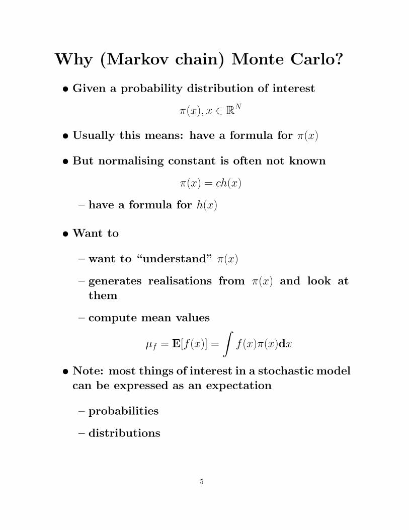
Why (Markov chain) Monte Carlo?
• Given a probability distribution of interest
π(x), x ∈ RN
• Usually this means: have a formula for π(x)
• But normalising constant is often not known
π(x) = ch(x)
– have a formula for h(x)
• Want to
– want to “understand” π(x)
– generates realisations from π(x) and look at
them
– compute mean values
µf = E[f(x)] =
∫f(x)π(x)dx
• Note: most things of interest in a stochastic model
can be expressed as an expectation
– probabilities
– distributions
5
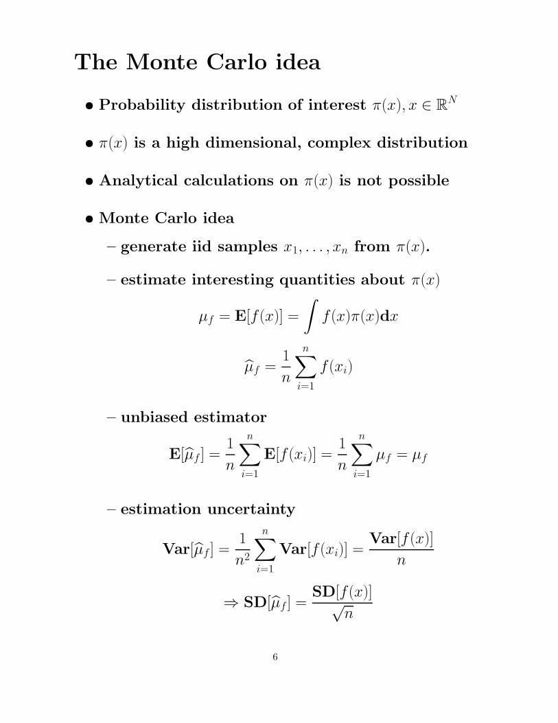
The Monte Carlo idea
• Probability distribution of interest π(x), x ∈ RN
• π(x) is a high dimensional, complex distribution
• Analytical calculations on π(x) is not possible
• Monte Carlo idea
– generate iid samples x1, . . . , xn from π(x).
– estimate interesting quantities about π(x)
µf = E[f(x)] =
∫f(x)π(x)dx
µf =1
n
n∑
i=1
f(xi)
– unbiased estimator
E[µf ] =1
n
n∑
i=1
E[f(xi)] =1
n
n∑
i=1
µf = µf
– estimation uncertainty
Var[µf ] =1
n2
n∑
i=1
Var[f(xi)] =Var[f(x)]
n
⇒ SD[µf ] =SD[f(x)]√
n
6

The Markov chain Monte Carlo idea
• Probability distribution of interest: π(x), x ∈ RN
• π(x) is a high dimensional, complex distribution
• Analytical calculations on π(x) is not possible
• Direct sampling from π(x) is not possible
• Markov chain Monte Carlo idea
– construct a Markov chain, Xi∞i=0, so that
limi→∞
P(Xi = x) = π(x)
– simulate the Markov chain for many iterations
– for m large enough, xm, xm+1, xm+2, . . . are (es-
sentially) samples from π(x)
– estimate interesting quantities about π(x)
µf = E[f(x)] =
∫f(x)π(x)dx
µf =1
n
m+n−1∑
i=m
f(xi)
– unbiased estimator
E[µf ] =1
n
m+n−1∑
i=m
E[f(xi)] =1
n
m+n−1∑
i=m
µf = µf
– what about the variance?
7

A (very) simple MCMC example
• Note: This is just for illustration, you should
never never use MCMC for this distribution!
• Let
π(x) =10x
x!e−10 , x = 0, 1, 2, . . .
0 5 10 15 20 25 30
0.0
0.1
0.2
0.3
• Set x0 to 0, 1 or 2 with probability 1/3 for each
• Markov chain kernel
P(xi+1 = xi − 1|xi) =
xi/20 if xi ≤ 9,
1/2 if xi > 9
P(xi+1 = xi|xi) =
(10 − xi)/20 if xi ≤ 9,
(xi − 9)/(2(xi + 1)) if xi > 9
P(xi+1 = xi + 1|xi) =
1/2 if xi ≤ 9,
5/(xi + 1) if xi > 9
• This Markov chain has limiting distribution π(x)
– will explain why later
8
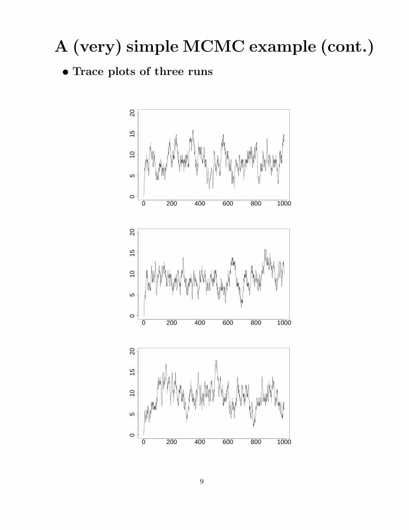
A (very) simple MCMC example (cont.)
• Trace plots of three runs
0 200 400 600 800 1000
05
1015
20
0 200 400 600 800 1000
05
1015
20
0 200 400 600 800 1000
05
1015
20
9
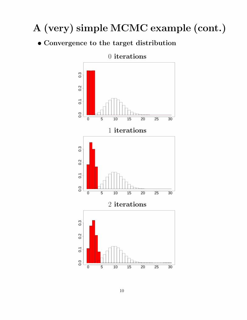
A (very) simple MCMC example (cont.)
• Convergence to the target distribution
0 iterations
0 5 10 15 20 25 30
0.0
0.1
0.2
0.3
1 iterations
0 5 10 15 20 25 30
0.0
0.1
0.2
0.3
2 iterations
0 5 10 15 20 25 30
0.0
0.1
0.2
0.3
10

A (very) simple MCMC example (cont.)
• Convergence to the target distribution
5 iterations
0 5 10 15 20 25 30
0.0
0.1
0.2
0.3
10 iterations
0 5 10 15 20 25 30
0.0
0.1
0.2
0.3
20 iterations
0 5 10 15 20 25 30
0.0
0.1
0.2
0.3
11
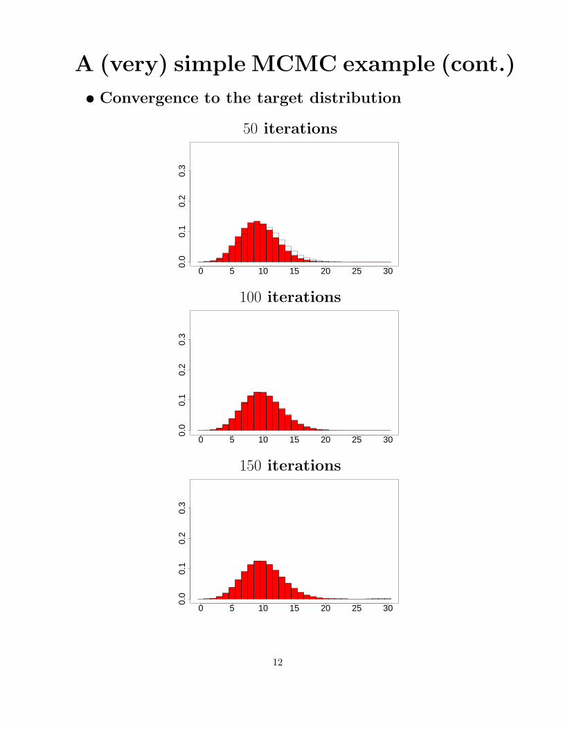
A (very) simple MCMC example (cont.)
• Convergence to the target distribution
50 iterations
0 5 10 15 20 25 30
0.0
0.1
0.2
0.3
100 iterations
0 5 10 15 20 25 30
0.0
0.1
0.2
0.3
150 iterations
0 5 10 15 20 25 30
0.0
0.1
0.2
0.3
12
Markov chain Monte Carlo
• Note:
– the chain x0, x1, x2, . . . is not converging!
– the distribution P(Xn = x) is converging
– we simulate/observe only the chain x0, x1, x2, . . .
• Need a (general) way to construct a Markov chain
for a given target distribution π(x).
• To simulate the Markov chain must be easy (or
at least possible)
• Need to decide when (we think) the chain has
converged (well enough)
13

Some Markov chain theory
• A Markov chain (x ∈ Ω discrete) is a discrete time
stochastic process Xi∞i=0, xi ∈ Ω which fulfils the
Markov assumption
PXi+1 = xi+1|X0 = x0, . . . , Xi = xi = PXi+1 = xi+1|Xi = xi
• Thus: a Markov chain can be specified by
– the initial distribution PX0 = x0 = g(x0)
– the transition kernel/matrix
P(y|x) = P(Xi+1 = y|Xi = x)
• Different notations are used
Pij Pxy P(x, y) P(y|x)
14

Some Markov chain theory
• A Markov chain (x ∈ Ω discrete) is defined by
– initial distribution: f(x0)
– transition kernel: P(y|x), note:∑
y∈Ω P (y|x) = 1
• Unique limiting distribution π(x) = limi→∞ f(xi) if
– chain is irreducible, aperiodic and positive re-
current
– if so, we have
π(y) =∑
x∈Ω
π(x)P(y|x) for all y ∈ Ω (1)
• Note: A sufficient condition for (1) is the detailed
balance condition
π(x)P(y|x) = π(y)P(x|y) for all x, y ∈ Ω
– proof:∑
x∈Ω
π(x)P(y|x) =∑
x∈Ω
π(y)P(x|y)
= π(y)∑
x∈Ω
P(x|y) = π(y)
• Note:
– in a stochastic modelling setting: P(y|x) is given,
want to find π(x)
– in an MCMC setting: π(x) is given, need to
find a P(y|x)
15

Implementation of the MCMC idea
• Given a (limiting distribution) π(x), x ∈ Ω
• Want a transition kernel so that
π(y) =∑
x∈Ω
π(x)P(y|x) for all y ∈ Ω
• Any solutions?
– # of unknowns: |Ω|(|Ω| − 1);
– # of equations: |Ω| − 1
• Difficult to construct P(y|x) from the above
• Require the detailed balance condition
π(x)P(y|x) = π(y)P(x|y) for all x, y ∈ Ω
• Any solutions:
– # of unknowns: |Ω|(|Ω| − 1)
– # of equations: |Ω|(|Ω| − 1)/2
• Still many solutions
• Recall: don’t need all solutions, one is enough!
• General (and easy) construction strategy for P(y|x)
is available → Metropolis–Hastings algorithm
16
Metropolis–Hastings algorithm
• Detailed balance condition
π(x)P(y|x) = π(y)P(x|y) for all x, y ∈ Ω
• Choose
P(y|x) = Q(y|x)α(y|x) for y 6= x,
where
– Q(y|x) is a proposal kernel, we can choose this
– α(y|x) ∈ [0, 1] is an acceptance probability, need
to find a formula for this
• Recall: must have∑
y∈Ω
P(y|x) = 1 for all x ∈ Ω
so then
P(x|x) = 1 −∑
y 6=x
Q(y|x)α(y|x)
• Simulation algorithm
– generate initial state x0 ∼ f(x0)
– for i = 1, 2, . . .
∗ propose potential new state yi ∼ Q(yi|xi−1)
∗ compute acceptance probability α(yi|xi−1)
∗ draw ui ∼ Uniform(0, 1)
∗ if ui ≤ α(yi|xi−1) accept yi, i.e. set xi = yi,
otherwise reject yi and set xi = xi−1
17
The acceptance probability• Recall: detailed balance condition
π(x)P(y|x) = π(y)P(x|y) for all x, y ∈ Ω
– Proposal kernel
P(y|x) = Q(y|x)α(y|x) for y 6= x
• Thus, must have
π(x)Q(y|x)α(y|x) = π(y)Q(x|y)α(x|y) for all x 6= y
• General solution
α(y|x) = r(x, y)π(y)Q(x|y) where r(x, y) = r(y, x)
• Recall: must have
α(y|x) = r(x, y)π(y)Q(x|y) ≤ 1 ⇒ r(x, y) ≤ 1
π(y)Q(x|y)
α(x|y) = r(x, y)π(x)Q(y|x) ≤ 1 ⇒ r(x, y) ≤ 1
π(x)Q(y|x)
• Choose r(x, y) as large as possible
r(x, y) = min
1
π(x)Q(y|x),
1
π(y)Q(x|y)
• Thus
α(y|x) = min
1,
π(y)Q(x|y)
π(x)Q(y|x)
18
Metropolis–Hastings algorithm
• Recall: For convergence it is sufficient with
– detailed balance
– irreducible
– aperiodic
– positive recurrent
• Detailed balance: ok by construction
• Irreducible: must be checked in each case
– usually easy
• Aperiodic: sufficient that P(x|x) > 0 for one x ∈ Ω
– for example by α(y|x) < 1 for one set x, y ∈ Ω
• Positive recurrent: in discrete state space, irre-
ducibility and finite state space is sufficient
– more difficult in general, but Markov chain
drifts if it is not recurrent
– usually not a problem in practice
19

Metropolis–Hastings algorithm
• Building blocks:
– target distribution π(x) (given by problem)
– proposal distribution Q(y|x) (we choose)
– acceptance probability
α(y|x) = min
1,
π(y)Q(x|y)
π(x)Q(y|x)
• Note: unknown normalising constant in π(x) ok
• A little history
– Metropolis et al. (1953). Equations of state
calculations by fast computing machines. J. of
Chemical Physics.
– Hastings (1970). Monte Carlo simulation meth-
ods using Markov chains and their applica-
tions. Biometrika.
– Green (1995). Reversible jump MCMC com-
putation and Bayesian model determination.
Biometrika.
20

A simple MCMC example (revisited)
• Let
π(x) =10x
x!e−10 , x = 0, 1, 2, . . .
0 5 10 15 20 25 30
0.0
0.1
0.2
0.3
• Proposal distribution
Q(y|x) =
1/2 for y ∈ x − 1, x + 1,0 otherwise
• Acceptance probability
y = x − 1 : α(x − 1|x) = min
1,
10x−1
(x−1)!e−10
10x
x! e−10
= min
1,
x
10
y = x + 1 : α(x + 1|x) = min
1,
10x+1
(x+1)!e−10
10x
x!e−10
= min
1,
10
x + 1
• P(y|x) then becomes as specified before
21
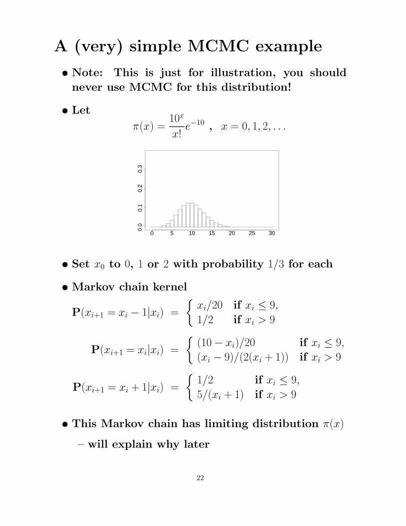
A (very) simple MCMC example
• Note: This is just for illustration, you should
never use MCMC for this distribution!
• Let
π(x) =10x
x!e−10 , x = 0, 1, 2, . . .
0 5 10 15 20 25 30
0.0
0.1
0.2
0.3
• Set x0 to 0, 1 or 2 with probability 1/3 for each
• Markov chain kernel
P(xi+1 = xi − 1|xi) =
xi/20 if xi ≤ 9,
1/2 if xi > 9
P(xi+1 = xi|xi) =
(10 − xi)/20 if xi ≤ 9,
(xi − 9)/(2(xi + 1)) if xi > 9
P(xi+1 = xi + 1|xi) =
1/2 if xi ≤ 9,
5/(xi + 1) if xi > 9
• This Markov chain has limiting distribution π(x)
– will explain why later
22

Another MCMC example — Ising
• 2D rectangular lattice of nodes
• Number the nodes from 1 to N
1 2 10
11 12
100
• xi ∈ 0, 1: value (colour) in node i, x = (x1, . . . , xN)
• First order neighbourhood
• Probability distribution
π(x) = c · exp
−β
∑
i∼j
I(xi 6= xj)
β: parameter; c: normalising constant,
c =
∑
x
exp
−β
∑
i∼j
I(xi 6= xj)
−1
23

Ising example (cont.)
• Probability distribution
π(x) = c · exp
−β
∑
i∼j
I(xi 6= xj)
• Proposal algorithm
– current state: x = (x1, . . . , xN)
– draw a node k ∈ 1, . . . , n at random
– propose to revers the value of node k, i.e.
y = (x1, . . . , xk−1, 1 − xk, xk+1, . . . , xN)
k
• Proposal kernel
Q(y|x) =
1N
if x and y differ in (exactly) one node,
0 otherwise
• Acceptance probability
α(y|x) = min
1,
π(y)Q(x|y)
π(x)Q(y|x)
= min
1, exp
−β
∑
j∼k
[I(xj 6= 1 − xk) − I(xj 6= xk)
]
24
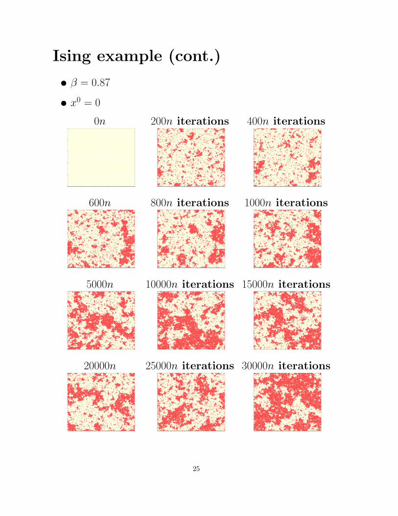
Ising example (cont.)
• β = 0.87
• x0 = 0
0n 200n iterations 400n iterations
600n 800n iterations 1000n iterations
5000n 10000n iterations 15000n iterations
20000n 25000n iterations 30000n iterations
25
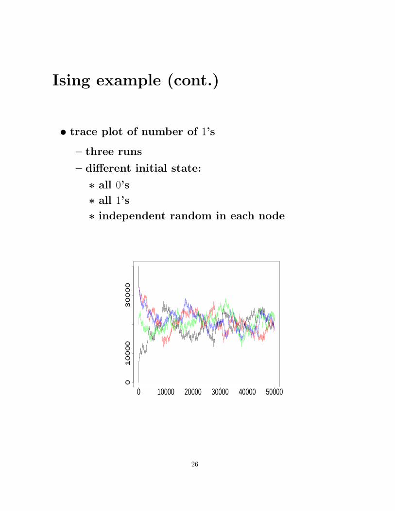
Ising example (cont.)
• trace plot of number of 1’s
– three runs
– different initial state:
∗ all 0’s
∗ all 1’s
∗ independent random in each node
0 10000 20000 30000 40000 50000
010000
30000
26

Continuous state space
• Target distribution
– discrete: π(x), x ∈ Ω
– continuous: π(x), x ∈ RN
• Proposal distribution
– discrete: Q(y|x)
– continuous: Q(y|x)
• Acceptance probability
– discrete: α(y|x)
– continuous: α(y|x)
α(y|x) = min
1,
π(y)Q(x|y)
π(x)Q(y|x)
• Rejection probability
– discrete:
r(x) = 1 −∑
y 6=x
Q(y|x)α(y|x)
– continuous:
r(x) = 1 −∫
RN
Q(y|x)α(y|x)dy
27
Plan
• The Markov chain Monte Carlo (MCMC) idea
• Some Markov chain theory
• Implementation of the MCMC idea
– Metropolis–Hastings algorithm
• MCMC strategies
– independent proposals
– random walk proposals
– combination of strategies
– Gibbs sampler
• Convergence diagnostics
– trace plots
– autocorrelation functions
– one chain or many chains?
• Typical MCMC problems — and some remedies
– high correlation between variables
– multimodality
– different scales
28