Introduction to MATLAB: Part I MATLAB is a software package that lets you do mathematics and computation, analyze data, develop algorithms, do simulation and modeling, and produce graphical displays and graphical user interfaces. This section will introduce you to how to use the MATLAB within the scope of physics laboratory experiments. The convention in this instruction is that a command in MATLAB is written in bold gray in the text. Installation of MATLAB on your own computer

If you wish to have MATLAB software installed on your own computer, you can download it from NJIT Information Services & Technology Department (visit URL of https://ist.njit.edu/matlab/). You can follow the installation instruction provided by the website.

Getting Started

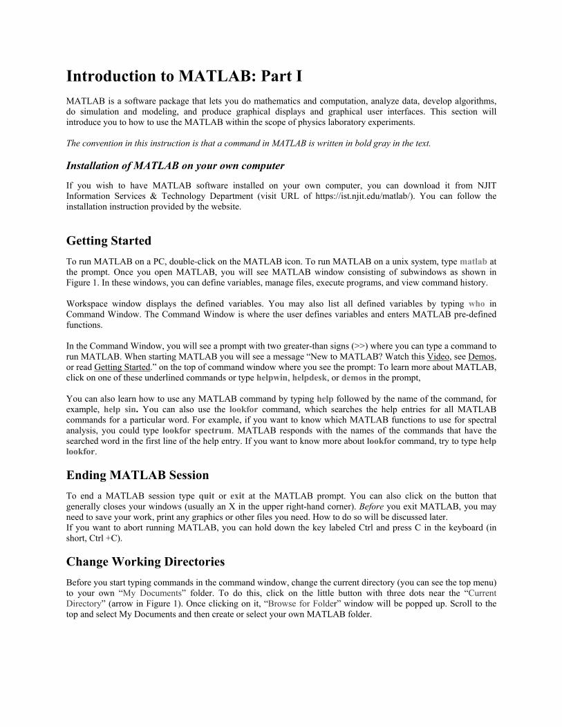
To run MATLAB on a PC, double-click on the MATLAB icon. To run MATLAB on a unix system, type matlab at the prompt. Once you open MATLAB, you will see MATLAB window consisting of subwindows as shown in Figure 1. In these windows, you can define variables, manage files, execute programs, and view command history. Workspace window displays the defined variables. You may also list all defined variables by typing who in Command Window. The Command Window is where the user defines variables and enters MATLAB pre-defined functions. In the Command Window, you will see a prompt with two greater-than signs (>>) where you can type a command to run MATLAB. When starting MATLAB you will see a message “New to MATLAB? Watch this Video, see Demos, or read Getting Started.” on the top of command window where you see the prompt: To learn more about MATLAB, click on one of these underlined commands or type helpwin, helpdesk, or demos in the prompt, You can also learn how to use any MATLAB command by typing help followed by the name of the command, for example, help sin. You can also use the lookfor command, which searches the help entries for all MATLAB commands for a particular word. For example, if you want to know which MATLAB functions to use for spectral analysis, you could type lookfor spectrum. MATLAB responds with the names of the commands that have the searched word in the first line of the help entry. If you want to know more about lookfor command, try to type help lookfor.

Ending MATLAB Session

To end a MATLAB session type quit or exit at the MATLAB prompt. You can also click on the button that generally closes your windows (usually an X in the upper right-hand corner). Before you exit MATLAB, you may need to save your work, print any graphics or other files you need. How to do so will be discussed later. If you want to abort running MATLAB, you can hold down the key labeled Ctrl and press C in the keyboard (in short, Ctrl +C).

Change Working Directories

Before you start typing commands in the command window, change the current directory (you can see the top menu) to your own “My Documents” folder. To do this, click on the little button with three dots near the “Current Directory” (arrow in Figure 1). Once clicking on it, “Browse for Folder” window will be popped up. Scroll to the top and select My Documents and then create or select your own MATLAB folder.

Figure 1. MATLAB Window

Inputting Commands

To input a command and execute it, just type it at the prompt (>>) in the Command Window and press “Enter” key in the keyboard. For example, to run simple calculation of 1 + 1, type 1 + 1 at the prompt and press enter key: >> 1 + 1 ans = 2 The “ans” in the above is now a variable that you can use again. If you want to multiply the answer by 4, type ans*4 at the prompt and press enter key. >> ans*4 ans = 8 In some cases, it is worthwhile to include comments at the end of a command and/or in the command line in the Command Window or especially in M-file. These comments might explain what is being done in the calculation, or might interpret the results of the calculation. In MATLAB, the percent sign (%) begins a comment; the rest of the line is not executed by MATLAB. See the following: >> 1+1 % this is demonstration for inputting a command ans = 2

Assigning Variables

Variables in matlab are named objects that are assigned using the equals sign = . They are limited to 31 characters and can contain upper and lowercase letters, any number of ‘_’ characters, and numerals. They may not start with a numeral. matlab is case sensitive: A and a are different variables. The following are valid matlab variable assignments: a = 1 Speed = 1500

Command Window

Work Space

Command History

kineticEnergy_inital = ½*m*v^2 name = ’John Smith’ The followings are invalid assignments. If you type invalid assignments, you get error message in MATLAB (see below): >> 2for1 = 3 ??? 2for1 = 3 Error: Unexpected MATLAB expression. first one = 1 To assign a variable without getting an echo from MATLAB end the assignment with a semi-colon (;). See the difference in the followings: >> speed = 10 MATLAB will display or echo your input of >>speed = 10 as below: speed = 10 To suppress the echo, add a “;” at the end of the input: >> speed = 10; The echo is not seen. In fact the variable of “speed” is stored in MATLAB. If you type speed, MATLAB will show the data assigned to the variable of speed: >> speed speed = 10

Inputting Vectors and Matrices

A vector is an ordered list of numbers. There are two types of vectors, row vector and column vector. For example, Row vector, A = (1 3 5 -1 0), which is 15 (number of rows number of columns) matrix and

which is 51 matrix. Column vector, You can enter a vector of any length in MATLAB by typing a list of numbers, separated by commas (,) and/or spaces, inside square brackets. For example: >> x= [-1,1,2,4,6] x = -1 1 2 4 6 >> y = [-2 0 -1 4 8] y = -2 0 -1 4 8 Suppose that you want to create a vector of values ranging from 1 to 10. Here’s how to do it without typing each number:

B

1

3

5

1

0

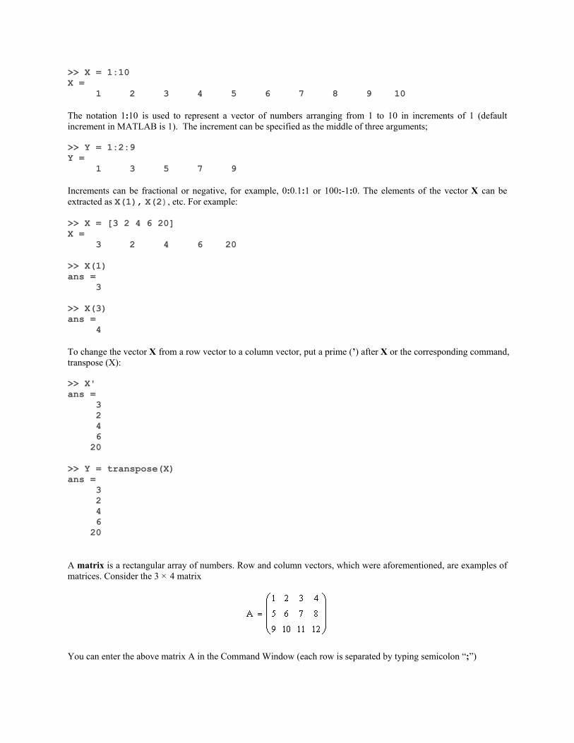
>> X = 1:10 X = 1 2 3 4 5 6 7 8 9 10 The notation 1:10 is used to represent a vector of numbers arranging from 1 to 10 in increments of 1 (default increment in MATLAB is 1). The increment can be specified as the middle of three arguments; >> Y = 1:2:9 Y = 1 3 5 7 9 Increments can be fractional or negative, for example, 0:0.1:1 or 100:-1:0. The elements of the vector X can be extracted as X(1), X(2), etc. For example: >> X = [3 2 4 6 20] X = 3 2 4 6 20 >> X(1) ans = 3 >> X(3) ans = 4 To change the vector X from a row vector to a column vector, put a prime (’) after X or the corresponding command, transpose (X): >> X' ans = 3 2 4 6 20 >> Y = transpose(X) ans = 3 2 4 6 20 A matrix is a rectangular array of numbers. Row and column vectors, which were aforementioned, are examples of matrices. Consider the 3 × 4 matrix

You can enter the above matrix A in the Command Window (each row is separated by typing semicolon “;”)

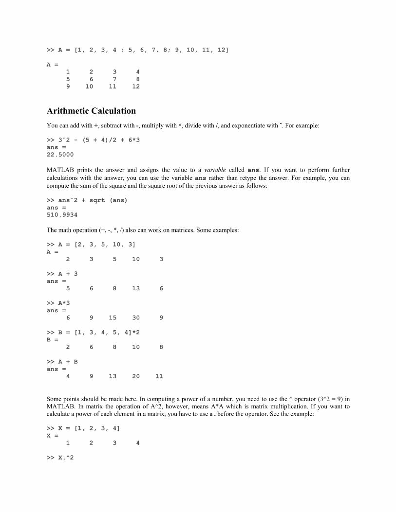
>> A = [1, 2, 3, 4 ; 5, 6, 7, 8; 9, 10, 11, 12] A = 1 2 3 4 5 6 7 8 9 10 11 12

Arithmetic Calculation

You can add with +, subtract with -, multiply with *, divide with /, and exponentiate with ˆ. For example: >> 3ˆ2 - (5 + 4)/2 + 6*3 ans = 22.5000 MATLAB prints the answer and assigns the value to a variable called ans. If you want to perform further calculations with the answer, you can use the variable ans rather than retype the answer. For example, you can compute the sum of the square and the square root of the previous answer as follows: >> ansˆ2 + sqrt (ans) ans = 510.9934 The math operation (+, -, *, /) also can work on matrices. Some examples: >> A = [2, 3, 5, 10, 3] A = 2 3 5 10 3 >> A + 3 ans = 5 6 8 13 6 >> A*3 ans = 6 9 15 30 9 >> B = [1, 3, 4, 5, 4]*2 B = 2 6 8 10 8 >> A + B ans = 4 9 13 20 11 Some points should be made here. In computing a power of a number, you need to use the ^ operator (3^2 = 9) in MATLAB. In matrix the operation of A^2, however, means A*A which is matrix multiplication. If you want to calculate a power of each element in a matrix, you have to use a . before the operator. See the example: >> X = [1, 2, 3, 4] X = 1 2 3 4 >> X.^2

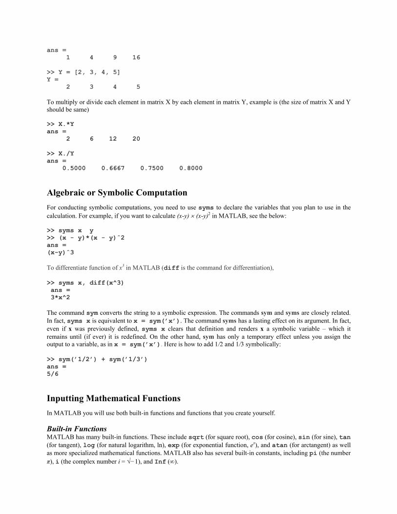
ans = 1 4 9 16 >> Y = [2, 3, 4, 5] Y = 2 3 4 5 To multiply or divide each element in matrix X by each element in matrix Y, example is (the size of matrix X and Y should be same) >> X.*Y ans = 2 6 12 20 >> X./Y ans = 0.5000 0.6667 0.7500 0.8000

Algebraic or Symbolic Computation

For conducting symbolic computations, you need to use syms to declare the variables that you plan to use in the calculation. For example, if you want to calculate (x-y) (x-y)2 in MATLAB, see the below: >> syms x y >> (x - y)*(x - y)ˆ2 ans = (x-y)ˆ3 To differentiate function of x3 in MATLAB (diff is the command for differentiation), >> syms x, diff(x^3) ans = 3*x^2 The command sym converts the string to a symbolic expression. The commands sym and syms are closely related. In fact, syms x is equivalent to x = sym(’x’). The command syms has a lasting effect on its argument. In fact, even if x was previously defined, syms x clears that definition and renders x a symbolic variable – which it remains until (if ever) it is redefined. On the other hand, sym has only a temporary effect unless you assign the output to a variable, as in x = sym(’x’). Here is how to add 1/2 and 1/3 symbolically: >> sym(’1/2’) + sym(’1/3’) ans = 5/6

Inputting Mathematical Functions

In MATLAB you will use both built-in functions and functions that you create yourself. Built-in Functions MATLAB has many built-in functions. These include sqrt (for square root), cos (for cosine), sin (for sine), tan (for tangent), log (for natural logarithm, ln), exp (for exponential function, ex), and atan (for arctangent) as well as more specialized mathematical functions. MATLAB also has several built-in constants, including pi (the number π), i (the complex number i = √−1), and Inf ().

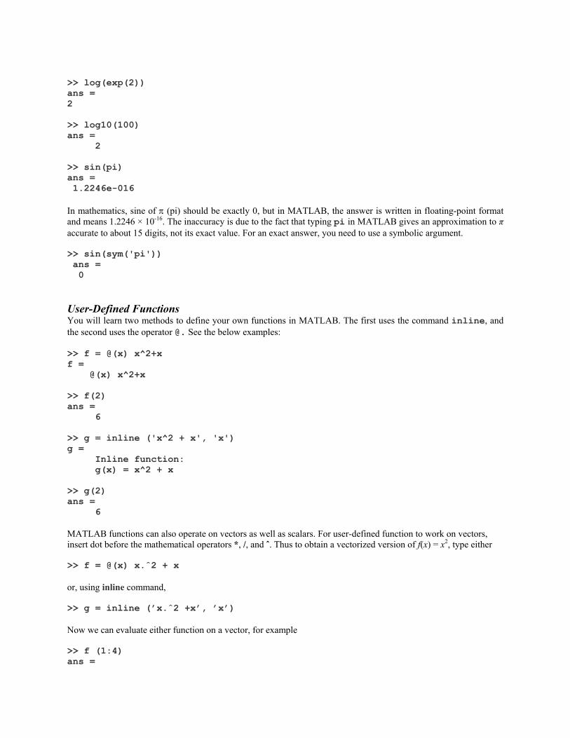
>> log(exp(2)) ans = 2 >> log10(100) ans = 2 >> sin(pi) ans = 1.2246e-016

In mathematics, sine of (pi) should be exactly 0, but in MATLAB, the answer is written in floating-point format and means 1.2246 × 10-16. The inaccuracy is due to the fact that typing pi in MATLAB gives an approximation to π accurate to about 15 digits, not its exact value. For an exact answer, you need to use a symbolic argument.

>> sin(sym('pi')) ans = 0 User-Defined Functions You will learn two methods to define your own functions in MATLAB. The first uses the command inline, and the second uses the operator @. See the below examples: >> f = @(x) x^2+x f = @(x) x^2+x >> f(2) ans = 6 >> g = inline ('x^2 + x', 'x') g = Inline function: g(x) = x^2 + x >> g(2) ans = 6 MATLAB functions can also operate on vectors as well as scalars. For user-defined function to work on vectors, insert dot before the mathematical operators *, /, and ˆ. Thus to obtain a vectorized version of f(x) = x2, type either >> f = @(x) x.ˆ2 + x or, using inline command, >> g = inline (’x.ˆ2 +x’, ’x’) Now we can evaluate either function on a vector, for example >> f (1:4) ans =

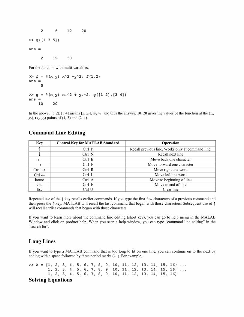
2 6 12 20 >> g([1 3 5]) ans = 2 12 30 For the function with multi-variables, >> f = @(x,y) x^2 +y^2; f(1,2) ans = 5 >> g = @(x,y) x.^2 + y.^2; g([1 2],[3 4]) ans = 10 20 In the above, [ 1 2], [3 4] means [x1 x2], [y1 y2] and thus the answer, 10 20 gives the values of the function at the (x1, y1), (x2, y2) points of (1, 3) and (2, 4).

Command Line Editing

Key Control Key for MATLAB Standard Operation

Ctrl P Recall previous line. Works only at command line. Ctrl N Recall next line Ctrl B Move back one character Ctrl F Move forward one character

Ctrl Ctrl R Move right one word Ctrl Ctrl L Move left one word home Ctrl A Move to beginning of line end Ctrl E Move to end of line Esc Ctrl U Clear line

Repeated use of the ↑ key recalls earlier commands. If you type the first few characters of a previous command and then press the ↑ key, MATLAB will recall the last command that began with those characters. Subsequent use of ↑ will recall earlier commands that began with those characters. If you want to learn more about the command line editing (short key), you can go to help menu in the MALAB Window and click on product help. When you seen a help window, you can type “command line editing” in the “search for”.

Long Lines If you want to type a MATLAB command that is too long to fit on one line, you can continue on to the next by ending with a space followed by three period marks (…). For example, >> A = [1, 2, 3, 4, 5, 6, 7, 8, 9, 10, 11, 12, 13, 14, 15, 16; ... 1, 2, 3, 4, 5, 6, 7, 8, 9, 10, 11, 12, 13, 14, 15, 16; ... 1, 2, 3, 4, 5, 6, 7, 8, 9, 10, 11, 12, 13, 14, 15, 16]

Solving Equations

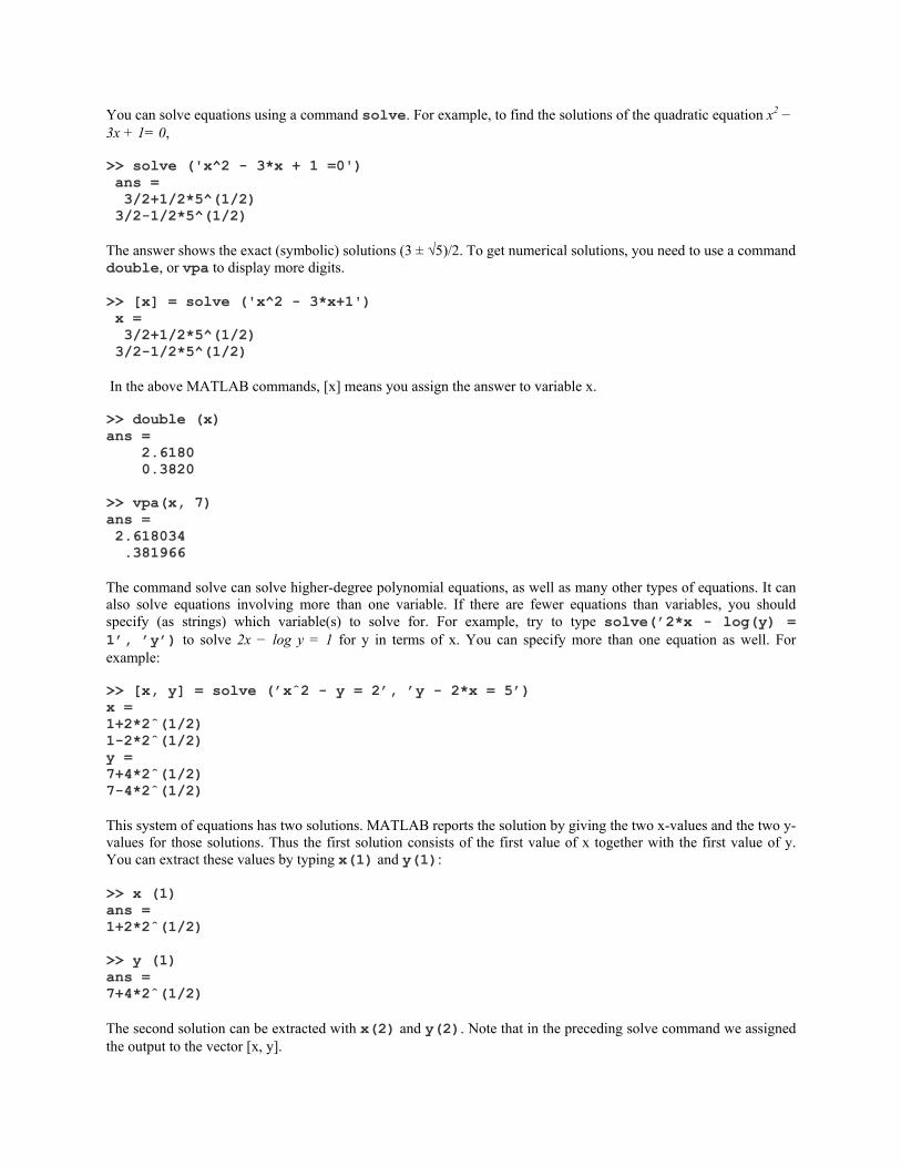
You can solve equations using a command solve. For example, to find the solutions of the quadratic equation x2 − 3x + 1= 0, >> solve ('x^2 - 3*x + 1 =0') ans = 3/2+1/2*5^(1/2) 3/2-1/2*5^(1/2) The answer shows the exact (symbolic) solutions (3 ± √5)/2. To get numerical solutions, you need to use a command double, or vpa to display more digits. >> [x] = solve ('x^2 - 3*x+1') x = 3/2+1/2*5^(1/2) 3/2-1/2*5^(1/2) In the above MATLAB commands, [x] means you assign the answer to variable x. >> double (x) ans = 2.6180 0.3820 >> vpa(x, 7) ans = 2.618034 .381966 The command solve can solve higher-degree polynomial equations, as well as many other types of equations. It can also solve equations involving more than one variable. If there are fewer equations than variables, you should specify (as strings) which variable(s) to solve for. For example, try to type solve(’2*x - log(y) = 1’, ’y’) to solve 2x − log y = 1 for y in terms of x. You can specify more than one equation as well. For example: >> [x, y] = solve (’xˆ2 - y = 2’, ’y - 2*x = 5’) x = 1+2*2ˆ(1/2) 1-2*2ˆ(1/2) y = 7+4*2ˆ(1/2) 7-4*2ˆ(1/2) This system of equations has two solutions. MATLAB reports the solution by giving the two x-values and the two y-values for those solutions. Thus the first solution consists of the first value of x together with the first value of y. You can extract these values by typing x(1) and y(1): >> x (1) ans = 1+2*2ˆ(1/2) >> y (1) ans = 7+4*2ˆ(1/2) The second solution can be extracted with x(2) and y(2). Note that in the preceding solve command we assigned the output to the vector [x, y].

Performing Calculus

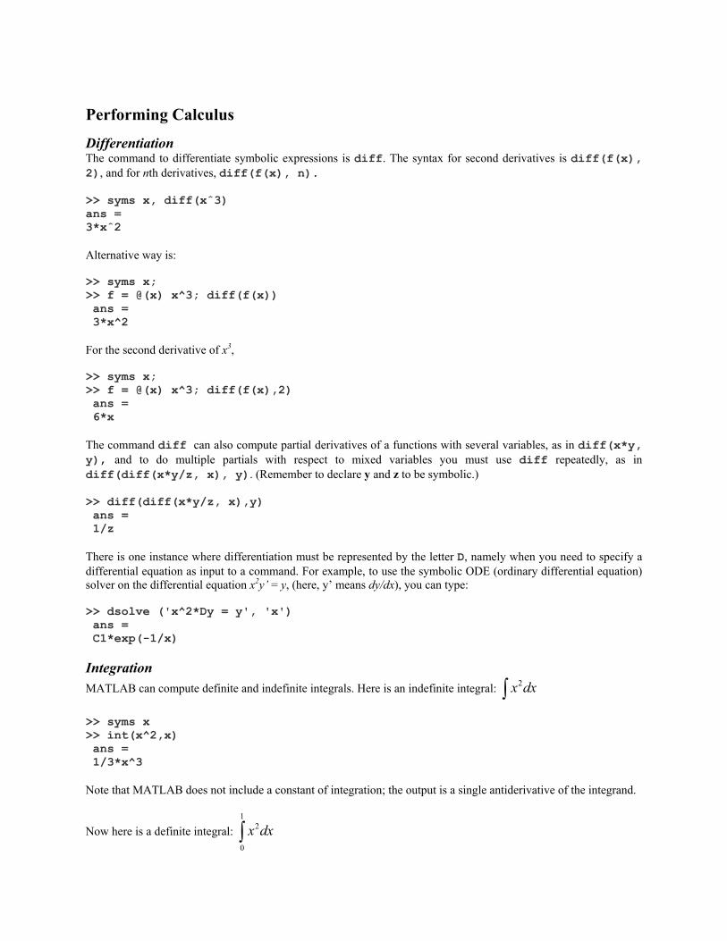
Differentiation The command to differentiate symbolic expressions is diff. The syntax for second derivatives is diff(f(x), 2), and for nth derivatives, diff(f(x), n). >> syms x, diff(xˆ3) ans = 3*xˆ2 Alternative way is: >> syms x; >> f = @(x) x^3; diff(f(x)) ans = 3*x^2 For the second derivative of x3, >> syms x; >> f = @(x) x^3; diff(f(x),2) ans = 6*x The command diff can also compute partial derivatives of a functions with several variables, as in diff(x*y, y), and to do multiple partials with respect to mixed variables you must use diff repeatedly, as in diff(diff(x*y/z, x), y). (Remember to declare y and z to be symbolic.) >> diff(diff(x*y/z, x),y) ans = 1/z There is one instance where differentiation must be represented by the letter D, namely when you need to specify a differential equation as input to a command. For example, to use the symbolic ODE (ordinary differential equation) solver on the differential equation x2y’ = y, (here, y’ means dy/dx), you can type: >> dsolve ('x^2*Dy = y', 'x') ans = C1*exp(-1/x) Integration

MATLAB can compute definite and indefinite integrals. Here is an indefinite integral: 2x dx

>> syms x >> int(x^2,x) ans = 1/3*x^3 Note that MATLAB does not include a constant of integration; the output is a single antiderivative of the integrand.

Now here is a definite integral: 1

2

0

x dx

>> int(x^2,x, 0,1) ans = 1/3 1

3

0

1x dx

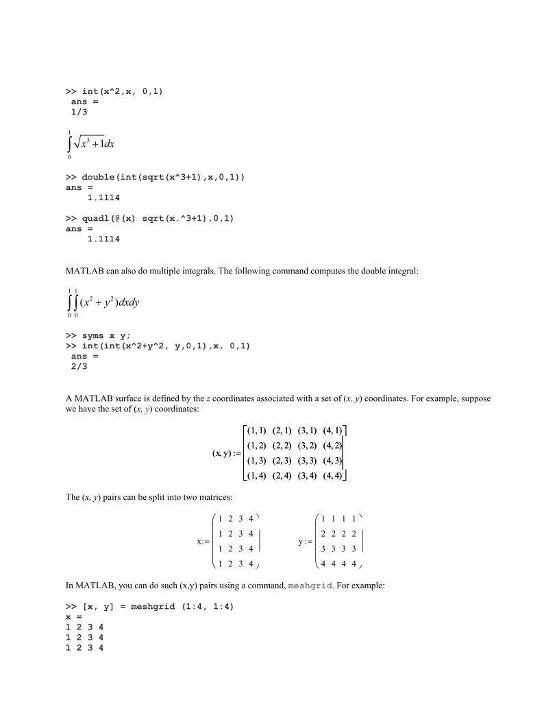
>> double(int(sqrt(x^3+1),x,0,1)) ans = 1.1114 >> quadl(@(x) sqrt(x.^3+1),0,1) ans = 1.1114 MATLAB can also do multiple integrals. The following command computes the double integral: 1 1

2 2

0 0

( )x y dxdy

>> syms x y; >> int(int(x^2+y^2, y,0,1),x, 0,1) ans = 2/3 A MATLAB surface is defined by the z coordinates associated with a set of (x, y) coordinates. For example, suppose we have the set of (x, y) coordinates:

x y( )

1 1( )

1 2( )

1 3( )

1 4( )

2 1( )

2 2( )

2 3( )

2 4( )

3 1( )

3 2( )

3 3( )

3 4( )

4 1( )

4 2( )

4 3( )

4 4( )

x y( )

1 1( )

1 2( )

1 3( )

1 4( )

2 1( )

2 2( )

2 3( )

2 4( )

3 1( )

3 2( )

3 3( )

3 4( )

4 1( )

4 2( )

4 3( )

4 4( )

The (x, y) pairs can be split into two matrices:

x

1

1

1

1

2

2

2

2

3

3

3

3

4

4

4

4

y

1

2

3

4

1

2

3

4

1

2

3

4

1

2

3

4

In MATLAB, you can do such (x,y) pairs using a command, meshgrid. For example: >> [x, y] = meshgrid (1:4, 1:4) x = 1 2 3 4 1 2 3 4 1 2 3 4

1 2 3 4 y = 1 1 1 1 2 2 2 2 3 3 3 3 4 4 4 4

The matrix x varies along its columns and y varies down its rows. We define the surface z: z x2

y2

x , which is

the distance of each (x, y) point from the origin (0, 0). To calculate z in MATLAB for the x and y matrices given above, we begin by using the meshgrid command to generates the required x and y matrices as shown above.

Now we simply convert our distance equation to MATLAB notation; z x2

y2

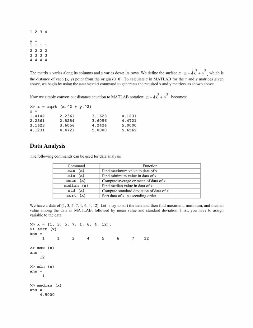
x becomes: >> z = sqrt (x.^2 + y.^2) z = 1.4142 2.2361 3.1623 4.1231 2.2361 2.8284 3.6056 4.4721 3.1623 3.6056 4.2426 5.0000 4.1231 4.4721 5.0000 5.6569

Data Analysis The following commands can be used for data analysis

Command Function max (x) Find maximum value in data of x min (x) Find minimum value in data of x mean (x) Compute average or mean of data of x median (x) Find median value in data of x std (x) Compute standard deviation of data of x sort (x) Sort data of x in ascending order

We have a data of (1, 3, 5, 7, 1, 6, 4, 12). Let ‘s try to sort the data and then find maximum, minimum, and median value among the data in MATLAB, followed by mean value and standard deviation. First, you have to assign variable to the data. >> x = [1, 3, 5, 7, 1, 6, 4, 12]; >> sort (x) ans = 1 1 3 4 5 6 7 12 >> max (x) ans = 12 >> min (x) ans = 1 >> median (x) ans = 4.5000

>> mean(x) ans = 4.8750 >> std(x) ans = 3.6031

Graphics

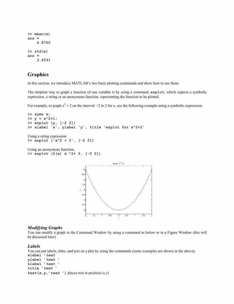
In this section, we introduce MATLAB’s two basic plotting commands and show how to use them. The simplest way to graph a function of one variable is by using a command, ezplot. which expects a symbolic expression, a string or an anonymous function, representing the function to be plotted. For example, to graph x2 + 2 on the interval −2 to 2 for x, see the following example using a symbolic expression: >> syms x; >> y = x^2+1; >> ezplot (y, [-2 2]) >> xlabel 'x', ylabel 'y', title 'ezplot for x^2+2' Using a string expression >> ezplot ('x^2 + 2', [-2 2]) Using an anonymous function, >> ezplot (@(x) x.^2+ 2, [-2 2])

Modifying Graphs You can modify a graph in the Command Window by using a command as below or in a Figure Window (this will be discussed later) . Labels You can put labels, titles, and text on a plot by using the commands (some examples are shown in the above): xlabel ’text ylabel ’text ’ zlabel ’text ’ title ’text ’ text(x,y,’text ’) places text at position (x,y)

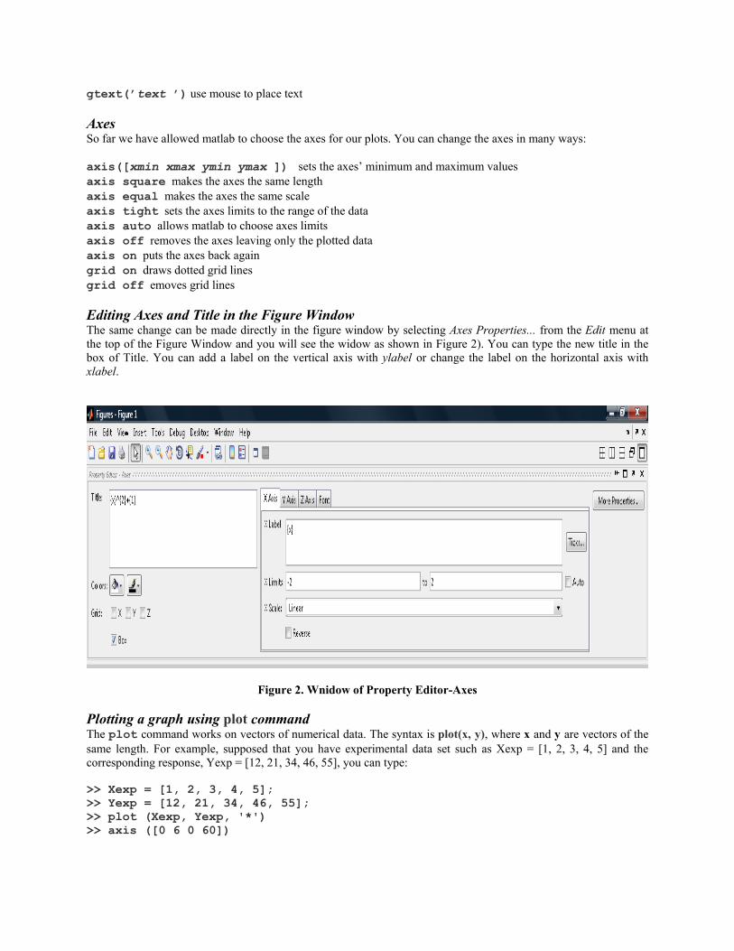
gtext(’text ’) use mouse to place text Axes So far we have allowed matlab to choose the axes for our plots. You can change the axes in many ways: axis([xmin xmax ymin ymax ]) sets the axes’ minimum and maximum values axis square makes the axes the same length axis equal makes the axes the same scale axis tight sets the axes limits to the range of the data axis auto allows matlab to choose axes limits axis off removes the axes leaving only the plotted data axis on puts the axes back again grid on draws dotted grid lines grid off emoves grid lines Editing Axes and Title in the Figure Window The same change can be made directly in the figure window by selecting Axes Properties... from the Edit menu at the top of the Figure Window and you will see the widow as shown in Figure 2). You can type the new title in the box of Title. You can add a label on the vertical axis with ylabel or change the label on the horizontal axis with xlabel.

Figure 2. Wnidow of Property Editor-Axes Plotting a graph using plot command The plot command works on vectors of numerical data. The syntax is plot(x, y), where x and y are vectors of the same length. For example, supposed that you have experimental data set such as Xexp = [1, 2, 3, 4, 5] and the corresponding response, Yexp = [12, 21, 34, 46, 55], you can type: >> Xexp = [1, 2, 3, 4, 5]; >> Yexp = [12, 21, 34, 46, 55]; >> plot (Xexp, Yexp, '*') >> axis ([0 6 0 60])

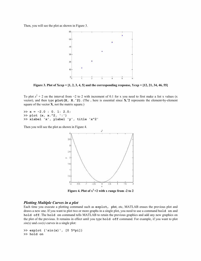
Then, you will see the plot as shown in Figure 3.

Figure 3. Plot of Xexp = [1, 2, 3, 4, 5] and the corresponding response, Yexp = [12, 21, 34, 46, 55]

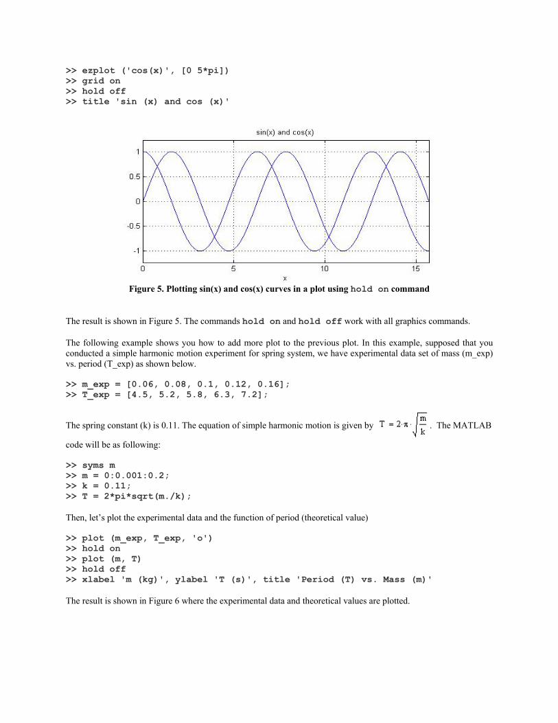
To plot x2 + 2 on the interval from −2 to 2 with increment of 0.1 for x you need to first make a list x values (x vector), and then type plot(X, X.ˆ2). (The . here is essential since X.ˆ2 represents the element-by-element square of the vector X, not the matrix square.) >> x = -2.0 : 0. 1: 2.0; >> plot (x, x.^2, ':') >> xlabel 'x', ylabel 'y', title 'x^2' Then you will see the plot as shown in Figure 4.

Figure 4. Plot of x2 +2 with x range from -2 to 2

Plotting Multiple Curves in a plot Each time you execute a plotting command such as ezplot, plot, etc, MATLAB erases the previous plot and draws a new one. If you want to plot two or more graphs in a single plot, you need to use a command hold on and hold off. The hold on command tells MATLAB to retain the previous graphics and add any new graphics on the plot of the previous. It remains in effect until you type hold off command. For example, if you want to plot sin(x) and cos(x) curves in a single plot: >> ezplot ('sin(x)', [0 5*pi]) >> hold on

>> ezplot ('cos(x)', [0 5*pi]) >> grid on >> hold off >> title 'sin (x) and cos (x)'

Figure 5. Plotting sin(x) and cos(x) curves in a plot using hold on command

The result is shown in Figure 5. The commands hold on and hold off work with all graphics commands. The following example shows you how to add more plot to the previous plot. In this example, supposed that you conducted a simple harmonic motion experiment for spring system, we have experimental data set of mass (m_exp) vs. period (T_exp) as shown below. >> m_exp = [0.06, 0.08, 0.1, 0.12, 0.16]; >> T_exp = [4.5, 5.2, 5.8, 6.3, 7.2];

The spring constant (k) is 0.11. The equation of simple harmonic motion is given by

. The MATLAB

code will be as following: >> syms m >> m = 0:0.001:0.2; >> k = 0.11; >> T = 2*pi*sqrt(m./k); Then, let’s plot the experimental data and the function of period (theoretical value) >> plot (m_exp, T_exp, 'o') >> hold on >> plot (m, T) >> hold off >> xlabel 'm (kg)', ylabel 'T (s)', title 'Period (T) vs. Mass (m)' The result is shown in Figure 6 where the experimental data and theoretical values are plotted.

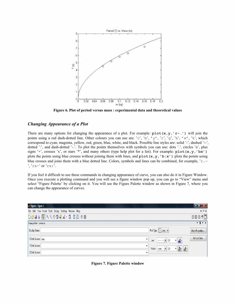
Figure 6. Plot of period versus mass : experimental data and theoretical values

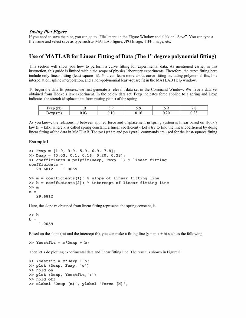
Changing Appearance of a Plot There are many options for changing the appearance of a plot. For example: plot(x,y,’r-.’) will join the points using a red dash-dotted line. Other colours you can use are: ’c’, ’m’, ’y’, ’r’, ’g’, ’b’, ’w’, ’k’, which correspond to cyan, magenta, yellow, red, green, blue, white, and black. Possible line styles are: solid ’-’, dashed ’--’, dotted ’:’, and dash-dotted ’-.’. To plot the points themselves with symbols you can use: dots ’.’, circles ’o’, plus signs ’+’, crosses ’x’, or stars ’*’, and many others (type help plot for a list). For example: plot(x,y,’bx’) plots the points using blue crosses without joining them with lines, and plot(x,y,’b:x’) plots the points using blue crosses and joins them with a blue dotted line. Colors, symbols and lines can be combined, for example, ’r.-’, ’rx-’ or ’rx:’. If you feel it difficult to use these commands in changing appearance of curve, you can also do it in Figure Window. Once you execute a plotting command and you will see a figure window pop up, you can go to “View” menu and select “Figure Palette’ by clicking on it. You will see the Figure Palette window as shown in Figure 7, where you can change the appearance of curves.

Figure 7. Figure Palette window

Saving Plot Figure If you need to save the plot, you can go to “File” menu in the Figure Window and click on “Save”. You can type a file name and select save as type such as MATLAb figure, JPG Image, TIFF Image, etc.

Use of MATLAB for Linear Fitting of Data (The 1st degree polynomial fitting) This section will show you how to perform a curve fitting for experimental data. As mentioned earlier in this instruction, this guide is limited within the scope of physics laboratory experiments. Therefore, the curve fitting here include only linear fitting (least-square fit). You can learn more about curve fitting including polynomial fits, line interpolation, spline interpolation, and a non-polynomial least-square fit in the MATLAB Help window. To begin the data fit process, we first generate a relevant data set in the Command Window. We have a data set obtained from Hooke’s law experiment. In the below data set, Fexp indicates force applied to a spring and Dexp indicates the stretch (displacement from resting point) of the spring.

Fexp (N) 1.9 3.9 5.9 6.9 7.8 Dexp (m) 0.03 0.10 0.16 0.20 0.23

As you know, the relationship between applied force and displacement in spring system is linear based on Hook’s law (F = kx, where k is called spring constant, a linear coefficient). Let’s try to find the linear coefficient by doing linear fitting of the data in MATLAB. The polyfit and polyval commands are used for the least-squares fitting. Example I >> Fexp = [1.9, 3.9, 5.9, 6.9, 7.8]; >> Dexp = [0.03, 0.1, 0.16, 0.20, 0.23]; >> coefficients = polyfit(Dexp, Fexp, 1) % linear fitting coefficients = 29.6812 1.0059 >> m = coefficients(1); % slope of linear fitting line >> b = coefficients(2); % intercept of linear fitting line >> m m = 29.6812 Here, the slope m obtained from linear fitting represents the spring constant, k. >> b b = 1.0059 Based on the slope (m) and the intercept (b), you can make a fitting line (y = mx + b) such as the following: >> Ybestfit = m*Dexp + b; Then let’s do plotting experimental data and linear fitting line. The result is shown in Figure 8. >> Ybestfit = m*Dexp + b; >> plot (Dexp, Fexp, 'o') >> hold on >> plot (Dexp, Ybestfit,':') >> hold off >> xlabel 'Dexp (m)', ylabel 'Force (N)',

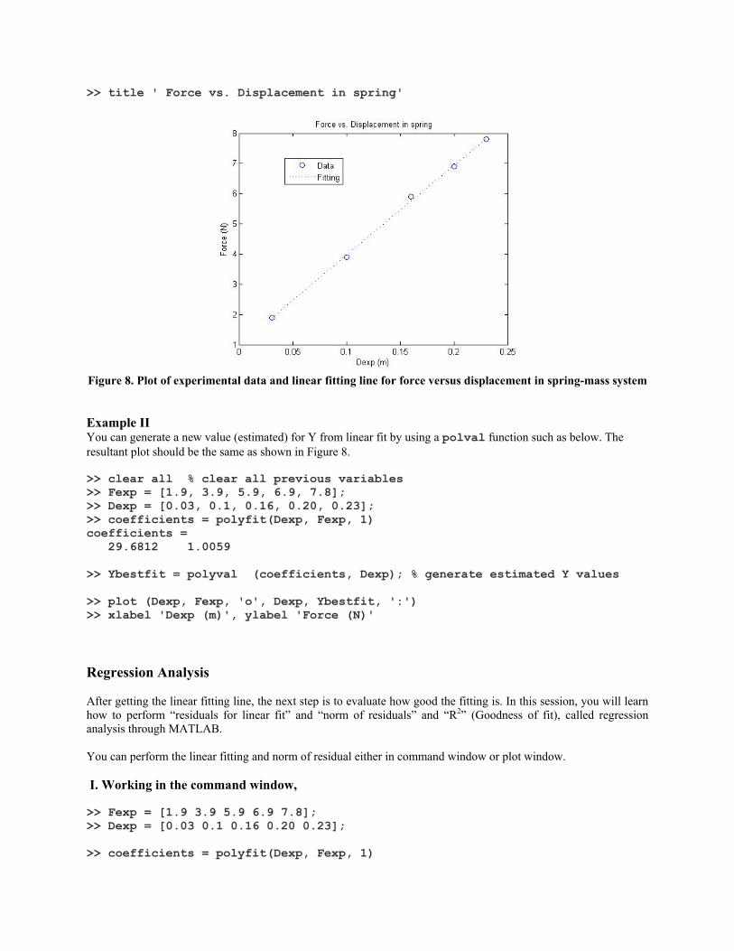
>> title ' Force vs. Displacement in spring'

Figure 8. Plot of experimental data and linear fitting line for force versus displacement in spring-mass system Example II You can generate a new value (estimated) for Y from linear fit by using a polval function such as below. The resultant plot should be the same as shown in Figure 8. >> clear all % clear all previous variables >> Fexp = [1.9, 3.9, 5.9, 6.9, 7.8]; >> Dexp = [0.03, 0.1, 0.16, 0.20, 0.23]; >> coefficients = polyfit(Dexp, Fexp, 1) coefficients = 29.6812 1.0059 >> Ybestfit = polyval (coefficients, Dexp); % generate estimated Y values >> plot (Dexp, Fexp, 'o', Dexp, Ybestfit, ':') >> xlabel 'Dexp (m)', ylabel 'Force (N)' Regression Analysis After getting the linear fitting line, the next step is to evaluate how good the fitting is. In this session, you will learn how to perform “residuals for linear fit” and “norm of residuals” and “R2” (Goodness of fit), called regression analysis through MATLAB. You can perform the linear fitting and norm of residual either in command window or plot window. I. Working in the command window, >> Fexp = [1.9 3.9 5.9 6.9 7.8]; >> Dexp = [0.03 0.1 0.16 0.20 0.23]; >> coefficients = polyfit(Dexp, Fexp, 1)

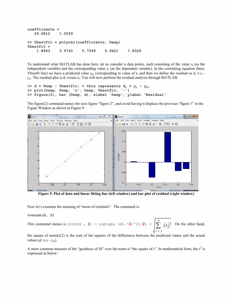
coefficients = 29.6812 1.0059 >> Ybestfit = polyval(coefficients, Dexp) Ybestfit = 1.8963 3.9740 5.7549 6.9421 7.8326 To understand what MATLAB has done here, let us consider n data points, each consisting of the value xi (as the independent variable) and the corresponding value yi (as the dependent variable). In the correlating equation (here, Ybestfit line) we have a predicted value ypi corresponding to value of xi and then we define the residual as di yi - ypi. The residual plot is di versus xi. You will now perform the residual analysis through MATLAB. >> d = Fexp - Ybestfit; % this represents di = yi – ypi >> plot(Dexp, Fexp, 'o', Dexp, Ybestfit, ':') >> figure(2), bar (Dexp, d), xlabel 'Dexp', ylabel 'Residual' The figure(2) command names the next figure “figure 2”, and avoid having it displace the previous “figure 1” in the Figure Window as shown in Figure 9.

Figure 9. Plot of data and linear fitting line (left window) and bar plot of residual (right window)

Now let’s examine the meaning of “norm of residuals”. The command is: >>norm(d, 2)

This command means is norm(d , 2) = sum(abs (d).^2)^(1/2) =

1

n

i

di 2

. On the other hand,

the square of norm(d,2) is the sum of the squares of the differences between the predicted values and the actual values (di yi - ypi). A more common measure of the “goodness of fit” over the norm is “the square of r”. In mathematical form, the r2 is expressed as below:

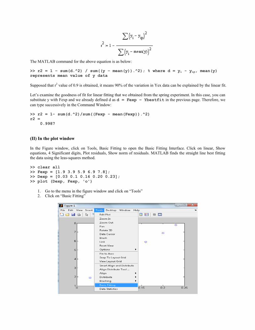
The MATLAB command for the above equation is as below: >> r2 = 1 – sum(d.^2) / sum((y – mean(y)).^2); % where d = yi - yip, mean(y) represents mean value of y data Supposed that r2 value of 0.9 is obtained, it means 90% of the variation in Yex data can be explained by the linear fit. Let’s examine the goodness of fit for linear fitting that we obtained from the spring experiment. In this case, you can substitute y with Fexp and we already defined d as d = Fexp – Ybestfit in the previous page. Therefore, we can type successively in the Command Window: >> r2 = 1- sum(d.^2)/sum((Fexp - mean(Fexp)).^2) r2 = 0.9987 (II) In the plot window In the Figure window, click on Tools, Basic Fitting to open the Basic Fitting Interface. Click on linear, Show equations, 4 Significant digits, Plot residuals, Show norm of residuals. MATLAB finds the straight line best fitting the data using the leas-squares method. >> clear all >> Fexp = [1.9 3.9 5.9 6.9 7.8]; >> Dexp = [0.03 0.1 0.16 0.20 0.23]; >> plot (Dexp, Fexp, 'o')

1. Go to the menu in the figure window and click on “Tools” 2. Click on “Basic Fitting”

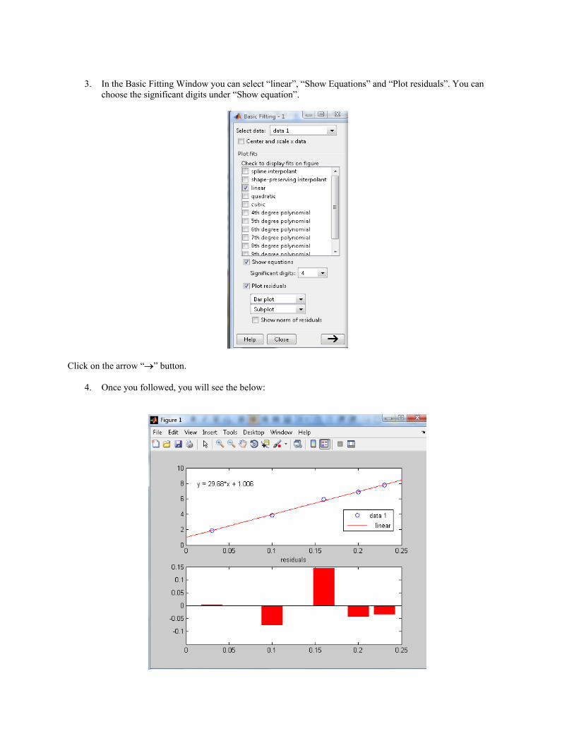
3. In the Basic Fitting Window you can select “linear”, “Show Equations” and “Plot residuals”. You can

choose the significant digits under “Show equation”.

Click on the arrow “” button.

4. Once you followed, you will see the below: