Introduction to Monte Carlo techniques and particle tracking

Luciano Pandola INFN

What Monte Carlo (MC) techniques are for?

Numerical solution of a (complex) macroscopic problem, by simulating the microscopic interactions among the components

Uses random sampling, until convergence is achieved Name after Monte Carlo's casino

Applications not only in physics and science, but also finances, traffic flow, social studies And not only problems that are intrisically

probabilistic (e.g. numerical integration)

An example: arrangement in an auditorium

Produce a configuration (or a "final state"), according to some "laws", e.g. People mostly arrive in pairs Audience members prefer an un-obstructed view of

the stage Audience members prefer seats in the middle, and

close to the front row Only one person can occupy a seat

Contrarily e.g. to physics, the laws are not known Rather use "working assumptions"

The math (exact) formulation can be impossible or unpratical MC is more effective

An example: arrangement in an auditorium

Reverse logic: find the "laws" that better fit the observed distribution Use MC to build a

(microscopic) theory of a complex system by comparison with experiments

MC in science

In physics, elementary laws are (typically) known MC is used to predict the outcome of a (complex) experiment Exact calculation from the basic laws is unpractical Optimize an experimental setup, support data

analysis Can be used to validate/disproof a theory, and/or

to provide small corrections to the theory In this course: Monte Carlo for particle tracking

(interaction of radiation with matter)

Interplay between theory, simulation and experiments

When are MC useful wrt to the math exact solution?

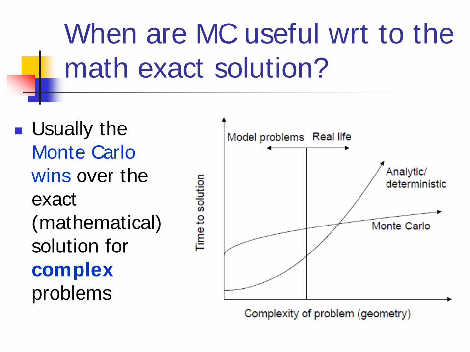
Usually the Monte Carlo wins over the exact (mathematical) solution for complex problems

A bit of history

Very concept of Monte Carlo comes in the XVIII century (Buffon, 1777, and then Laplace, 1786) Monte Carlo estimate of π

Concept of MC is much older than real computers one can also implement the

algorithms manually, with dice (= Randon Number Generator)

A bit of history

Boost in the '50 (Ulam and Von Neumann) for the development of thermonuclear weapons

Von Neumann invented the name "Monte Carlo" and settled a number of basic theorems

First (proto)computers available at that time MC mainly CPU load, minimal

I/O

The simplest MC application: numerical estimate of π

Shoot N couples (x,y) randomly in [0,1]

Count n: how many couples satisfy (x2+y2≤1)

[0,1]

[0,1]

n/N = π/4 (ratio of areas) Convergence as 1/ √N

Most common application in particle physics: particle tracking

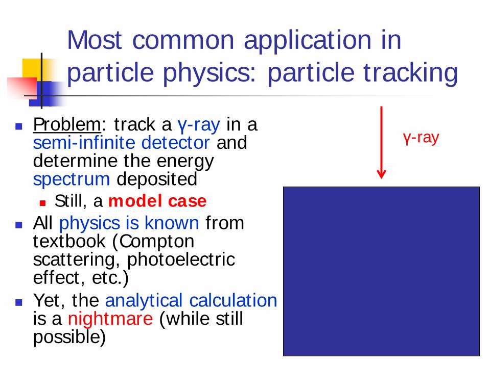
Problem: track a γ-ray in a semi-infinite detector and determine the energy spectrum deposited Still, a model case

All physics is known from textbook (Compton scattering, photoelectric effect, etc.)

Yet, the analytical calculation is a nightmare (while still possible)

γ-ray

Most common application in particle physics: particle tracking

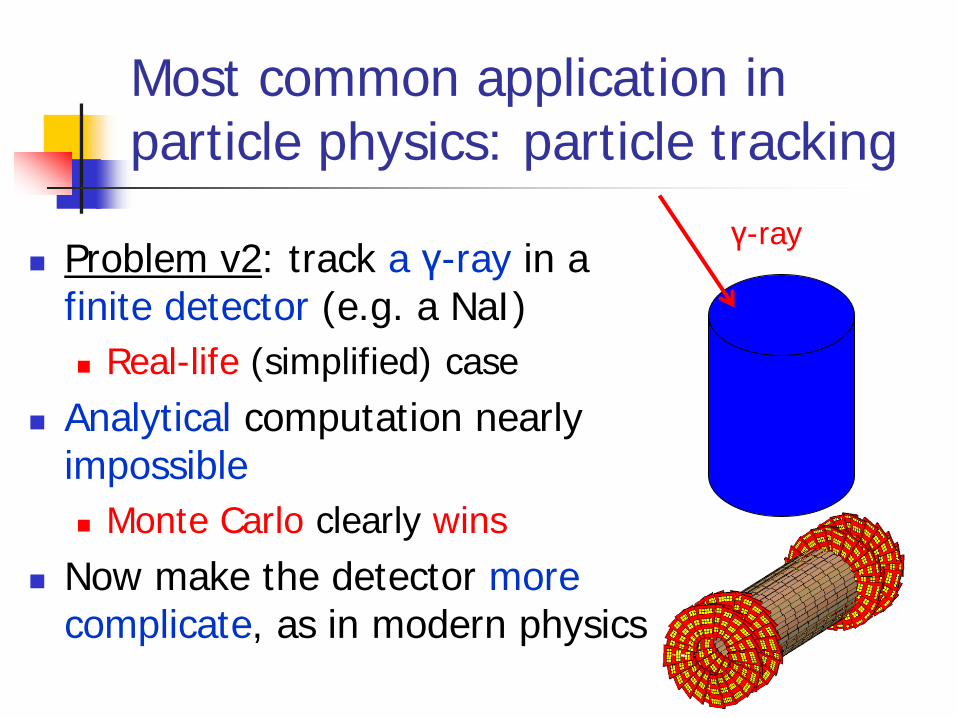
Problem v2: track a γ-ray in a finite detector (e.g. a NaI) Real-life (simplified) case

Analytical computation nearly impossible Monte Carlo clearly wins

Now make the detector more complicate, as in modern physics

γ-ray

Particle tracking

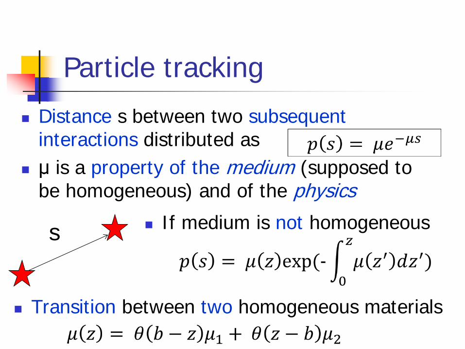
Distance s between two subsequent interactions distributed as

μ is a property of the medium (supposed to be homogeneous) and of the physics

s If medium is not homogeneous

Transition between two homogeneous materials

Particle tracking

μ is proportional to the total cross section and depends on the density of the material

s All competing processes

contribute with their own μi

Each process takes place with probability μi/μ i.e. proportionally to the partial cross sections

Particle tracking: basic recipe Divide the trajectory of the particle in "steps"

Straight free-flight tracks between consecutive physics interactions

Steps can also be limited by geometry boundaries Decide the step length s, by sampling according to

p(s)= μe-μs, with the proper μ (material+physics) Decide which interaction takes place at the end of the

step, according to μi/μ Produce the final state according to the physics of the

interaction (d2σ/dΩdE) Update direction of the primary particle Store somewhere the possible secondary particles, to be

tracked later on

Particle tracking: basic recipe

Follow all secondaries, until absorbed or leave volume Notice: μ depends on energy (cross sections do!)

s1

γ, E

s2

γ, E1

e-, E2

s3

γ, E3

e-, E4 e-, E5

Well, not so easy This basic recipe works fine for γ-rays and other

neutral particles (e.g. neutrons) Not so well for e±: the cross section (ionization &

bremsstrahlung) is very high, so the steps between two consecutive interactions are very small CPU intensive: viable for low energies and thin material

Even worse: in each interaction only a small fraction of energy is lost, and the angular displacement is small A lot of time is spent to simulate interactions having

small effect The interactions of γ are "catastrophics": large change

in energy/direction

Solution: the mixed Monte Carlo

Simulate explicitly (i.e. force step) interactions only if energy loss (or change of direction) is above threshold W0 Detailed simulation "hard" interaction (like γ interactions)

The effect of all sub-threshold interactions is described cumulatively Condensed simulation "soft" interactions

Hard interactions occur much less frequently than soft interactions Fully detailed simulation restored for W0=0

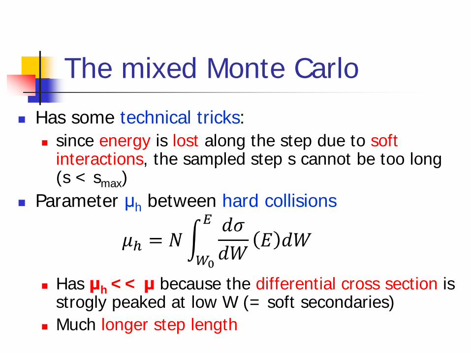
The mixed Monte Carlo

Has some technical tricks: since energy is lost along the step due to soft

interactions, the sampled step s cannot be too long (s < smax)

Parameter μh between hard collisions

Has μh << μ because the differential cross section is strogly peaked at low W (= soft secondaries)

Much longer step length

The mixed Monte Carlo

Stopping power due to soft collisions (dE/dx)

Average energy lost along the step: <w>=sSs Must be <w> << E

Fluctuations around the average value <w> have to be taken into account Appropriate random sampling of w with mean

value <w> and variance (straggling)

Extended recipe 1. Decide the step length s, by sampling according to

p(s)= μhe-μhs, with the proper μh

2. Calculate the cumulative effect of the soft interactions along the step: sample the energy loss w, with <w>=sSs, and the displacement

3. Update energy and direction of the primary particle at the end of the step E E-w

4. Decide which interaction takes place at the end of the step, according to μi,h/μh

5. Produce the final state according to the physics of the interaction (d2σ/dΩdE)

Particle tracking: mixed recipe

Follow all secondaries, until absorbed or leave volume

s1 (E)

e-, E

e-, E-w

<w> = Sss1

e-, E1

s2

e-, E2

<w> = Sss2

e-, E1-w e-, E3

γ, E4

s3

Geometry

Geometry also enters into the tracking A step can never cross a geometry boundary Always stop the step when there is a boundary,

then re-start in the new medium Navigation in the geometry can be CPU-intensive

One must know to which volume each point (x,y,z) belongs to, and how far (and in which direction) is the closest boundary

Trajectories can be affected also by EM fields, for charged particles

…luckily enough, somebody else already implemented the tracking algorithms for us (and much more)

Geant4 and the Geant4 Collaboration

Monte Carlo codes on the market

MCNP (neutrons mainly)

Penelope (e- and gamma)

PETRA (protons)

EGSnrc (e- and gammas)

PHIT (protons/ions)

FLUKA (any particle)

Geant4

-GEometry ANd Traking

-Geant4 - a simulation toolkit Nucl. Inst. and Methods Phys. Res. A, 506 250-303

-Geant4 developments and applications Transaction on Nuclear Science 53, 270-278

Facts about

Developed by an International Collaboration Established in 1998 Approximately 100 members, from Europe, US and

Japan http://geant4.org

Written in C++ language Takes advantage from the Object Oriented software

technology Open source Typically two releases per year

Major release, minor release, beta release

Basic concept of Geant4

Minimal software requirements

C++ A basic knowledge is required being Geant4 a collection

of C++ libraries It is complex but also no C++ experts can use Geant4

Object oriented technology (OO) Very basic knowledge Expertise needed for the development of complex

applications Unix/Linux

These are the standard OSs for Geant4 and a basic knowledge is required

How to compile a program, how to install from source code

Toolkit and User Application Geant4 is a toolkit (= a collection of tools)

i.e. you cannot “run” it out of the box You must write an application, which uses Geant4 tools

Consequences:

There are no such concepts as “Geant4 defaults” You must provide the necessary information to configure your

simulation You must deliberately choose which Geant4 tools to use

Guidance: many examples are provided

Basic Examples: overview of Geant4 tools Advanced Examples: Geant4 tools in real-life applications

Basic concepts

What you MUST do: Describe your experimental set-up Provide the primary particles input to your simulation Decide which particles and physics models you want to use

out of those available in Geant4 and the precision of your simulation (cuts to produce and track secondary particles)

You may also want To interact with Geant4 kernel to control your simulation To visualise your simulation configuration or results To produce histograms, tuples etc. to be further analysed

Main Geant4 capabilities

Transportation of a particle ‘step-by-step’ taking into account all possible interactions with materials and fields

The transport ends if the particle is slowed down to zero kinetic energy (and it doesn't have

any interaction at rest) disappears in some interaction reaches the end of the simulation volume

Geant4 allows the User to access the transportation process and retrieve the results (USER ACTIONS) at the beginning and end of the transport at the end of each step in transportation if a particle reaches a sensitive detector Others…

Multi-thread mode Geant4 10.0 (released Dec, 2013) supports multi-

thread approach for multi-core machines Simulation is automatically split on an event-by-

event basis different events are processed by different cores

Can fully profit of all cores available on modern machines substantial speed-up of simulations

Unique copy (master) of geometry and physics All cores have them as read-only (saves memory)

Backwards compatible with the sequential mode The MT programming requires some care: need to

avoid conflicts between threads Some modification and porting required

Who/why is using Geant4?

Experiments and MC In my knowledge, all experiments have a (more

or less detailed) full-scale Monte Carlo simulation Design phase

Evaluation of background Optimization of setup to maximize scientific yield

Minimize background, maximize signal efficiency

Running/analysis phase Support of data analysis (e.g. provide efficiency for

signal, background, coincidences, tagging, …). often, Monte Carlo is the only way to convert relative

rates (events/day) in absolute yields

Why Geant4 is a common choice in the market

Open source and object oriented/C++ No black box Freely available on all platforms Can be easily extended and customized by using the

existing interfaces New processes, new primary generators, interface to ROOT

analysis, … Can handle complex geometries Regular development, updates, bug fixes and

validation Good physics, customizable per use-cases End-to-end simulation (all particles, including optical

photons)

LHC @ CERN All four big LHC

experiments have a Geant4 simulation M of volumes Physics at the TeV scale

ATLAS

CMS

Benchmark with test-beam data

Key role for the Higgs searches

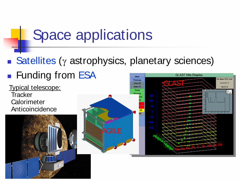
Space applications

Satellites (γ astrophysics, planetary sciences) Funding from ESA

AGILE

GLAST Typical telescope: Tracker Calorimeter Anticoincidence

Treatment planning for hadrontherapy and proton-therapy systems Goal: deliver dose to the tumor

while sparing the healthy tissues Alternative to less-precise (and

commercial) TP software Medical imaging Radiation fields from medical

accelerators and devices medical_linac gamma-knife brachytherapy

Proton-therapy beam line

GEANT4 simulation

Medical applications

Dosimetry with Geant4

Space science Radiotherapy Effects on electronics components

Nuclear spectroscopy

41 SCEPTAR

TIGRESS

Low background experiments Neutrinoless ββ

decay: GERDA, Majorana

COBRA, CUORE, EXO

Dark matter detection: Zeplin-II/III, Drift, Edelweiss, ArDM,

Xenon, CRESST, Lux, Elixir,

Solar neutrinos: Borexino, ...

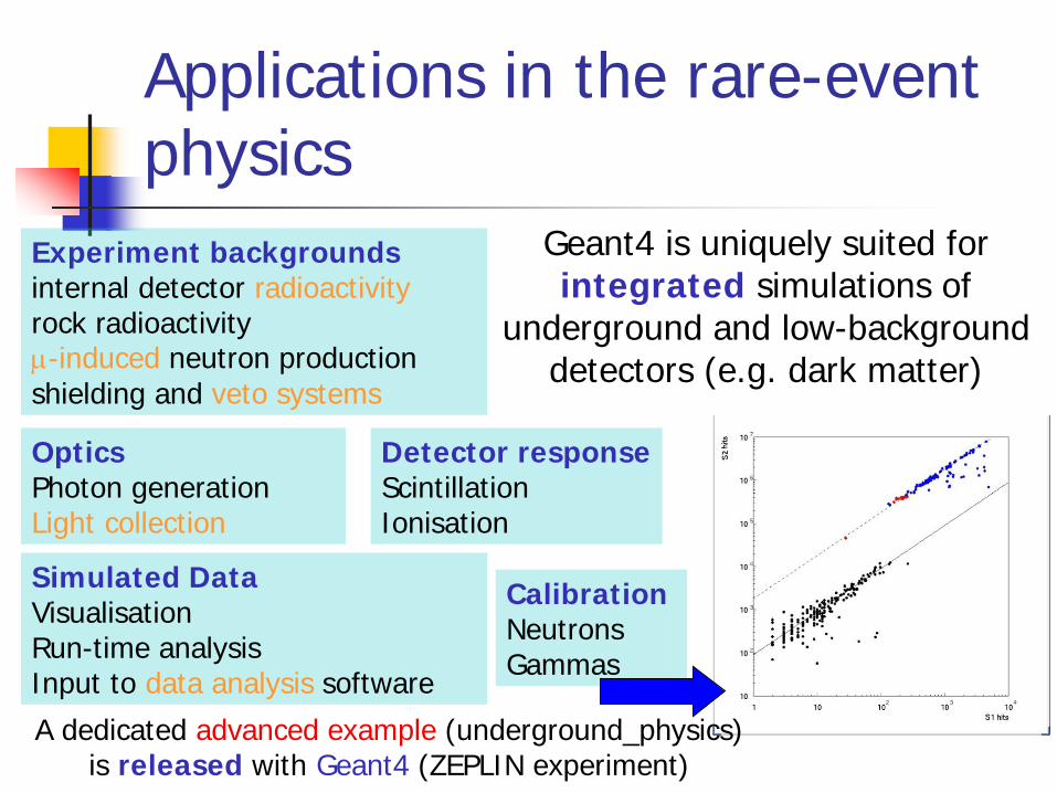
Applications in the rare-event physics

Experiment backgrounds internal detector radioactivity rock radioactivity µ-induced neutron production shielding and veto systems

Calibration Neutrons Gammas

Optics Photon generation Light collection

Detector response Scintillation Ionisation

Simulated Data Visualisation Run-time analysis Input to data analysis software

Geant4 is uniquely suited for integrated simulations of

underground and low-background detectors (e.g. dark matter)

A dedicated advanced example (underground_physics) is released with Geant4 (ZEPLIN experiment)

Geant4-based frameworks in astroparticle/neutrino physics

Geant4 is a toolkit can be used in software projects of wider scope Flexibility in selecting geometries, physics, outputs, …

A few examples in astroparticle physics: MaGe (GERDA/Majorana): double beta decay LUXSim (LUX): dark matter and undeground experiments DCGLG4sim (Double Chooz): liquid scintillator and reactor

neutrinos artG4 (FermiLab) VENOM (COBRA): double beta decay Just google "Geant4-based"

(Many more for HEP, space physics, medical physics)

Geant4-based frameworks in the medical physics

TOPAS

PTSim

GATE

Gallery