sampling methods, particle filtering, and markov-chain monte carlo

CSE598CRobert Collins

Sampling Methods, Particle Filtering, and Markov-Chain Monte Carlo

CSE598C Vision-Based TrackingFall 2012, CSE Dept, Penn State Univ


References


Recall: Bayesian Filtering

Rigorous general framework for tracking. Estimates the values of a state vector based on a time series of uncertain observations.

Key idea: use a recursive estimator to construct the posterior density function (pdf) of the state vector at each time t based on all available data up to time t.

Bayesian hypothesis: All quantities of interest, such as MAP or marginal estimates, can be computed from the posterior pdf.


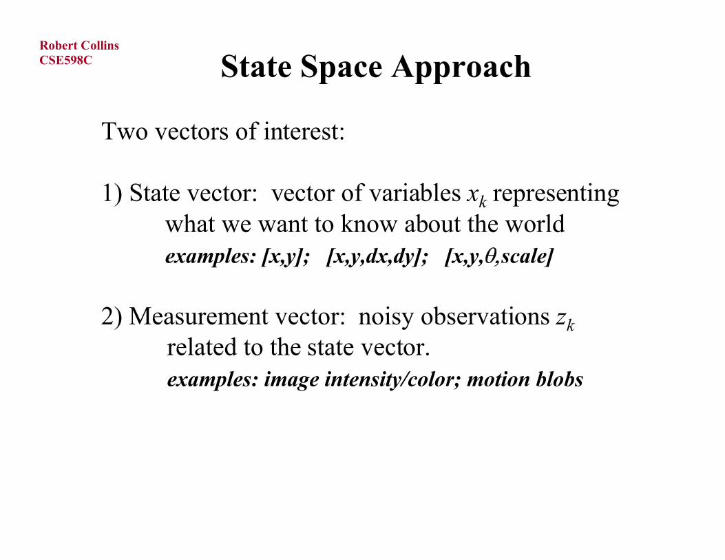
State Space Approach

Two vectors of interest:

1) State vector: vector of variables xk representingwhat we want to know about the worldexamples: [x,y]; [x,y,dx,dy]; [x,y,scale]

2) Measurement vector: noisy observations zk

related to the state vector. examples: image intensity/color; motion blobs


Discrete Time Models

Discrete Time Formulation - measurements becomeavailable at discrete time steps 1,2,3,..,k,...(very appropriate for video processing applications)

Need to specify two models:1) System model - how current state is related to previous

state (specifies evolution of state with time)xk = fk (xk-1, vk-1) v is process noise

2) Measurement model - how noisy measurements arerelated to the current state

zk = hk (xk, nk) n is measurement noise


Recursive Filter

We want to recursively estimate the current stateat every time that a measurement is received.

Two step approach:

1) prediction: propagate state pdf forward in time,taking process noise into account (translate, deform, and spread the pdf)

2) update: use Bayes theorem to modify prediction pdf based on current measurement


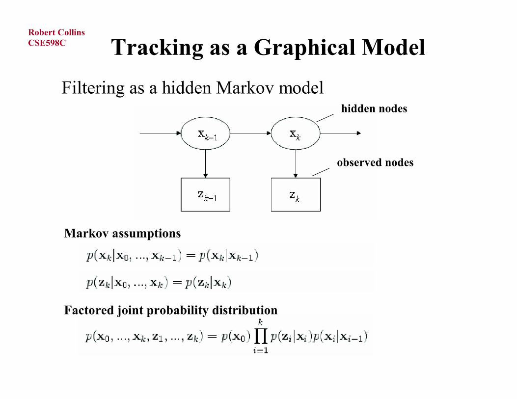
Tracking as a Graphical Model

Filtering as a hidden Markov modelhidden nodes

observed nodes

Markov assumptions

Factored joint probability distribution


Recursive Bayes Filter

Motion Prediction Step:

Data Correction Step (Bayes rule):

previous estimated statestate transitionpredicted current state

predicted current statemeasurementestimated current state

normalization term


Problem

Except in special cases, these integrals are intractible.



(examples of special cases: linear+Gaussian (Kalman); discrete state spaces)


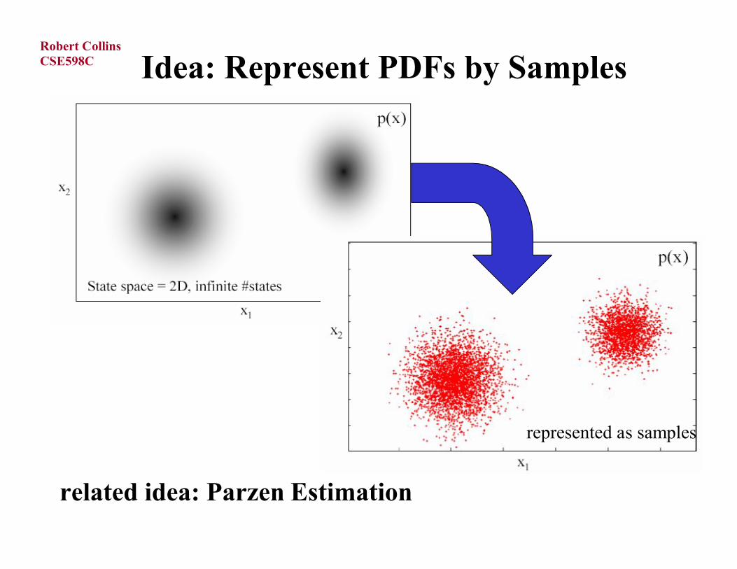
Idea: Represent PDFs by Samples

related idea: Parzen Estimation

represented as samples


Why Does This Help?

If we can generate random samples xi from a given distribution P(x), then we can estimate expected values of functions under this distribution by summation, rather than integration.

That is, we can approximate:

by first generating N i.i.d. samples from P(x) and then forming the empirical estimate:

related idea: Monte Carlo Integration


A Brief Overview of Sampling

Inverse Transform Sampling (CDF)

Rejection Sampling

Importance Sampling


Inverse Transform Sampling

It is easy to sample from a discrete 1D distribution, using the cumulative distribution function.

1 N

wk

k 1 Nk

1

0



It is easy to sample from a discrete 1D distribution, using the cumulative distribution function.

1 Nk

1

0

1) Generate uniform u in the range [0,1]

u

2) Visualize a horizontal line intersecting bars

3) If index of intersected bar is j, output new sample xj j

xj



Why it works:

inverse cumulative distribution function

cumulative distribution function


Efficient Generating Many Samples

Basic idea: choose one initial small random number; deterministically sample the rest by “crawling” up the cdf function. This is O(N).

from Arulampalam paper

odd property: you generate the “random”numbers in sorted order...


A Brief Overview of Sampling

Inverse Transform Sampling (CDF)

Rejection Sampling

Importance Sampling

For these two, we can sample from continuous distributions, and they do not even need to be normalized.

That is, to sample from distribution P, we only need to know a function P*, where P = P* / c , for some normalization constant c.


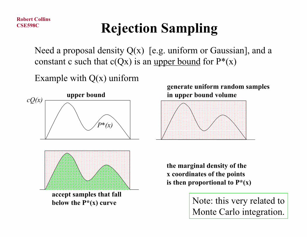
Rejection Sampling

Need a proposal density Q(x) [e.g. uniform or Gaussian], and a constant c such that c(Qx) is an upper bound for P*(x)

Example with Q(x) uniformgenerate uniform random samples in upper bound volumeupper bound

cQ(x)

P*(x)

accept samples that fallbelow the P*(x) curve

the marginal density of thex coordinates of the pointsis then proportional to P*(x)

Note: this very related toMonte Carlo integration.


Rejection Sampling

More generally:

1) generate sample xi from a proposal density Q(x)

2) generate sample u from uniform [0,cQ(xi)]

3) if u <= P*(xi) accept xi; else reject

Q(x)

cQ(xi)u

P*(x)cQ(x)

xi

reject

u accept


Importance “Sampling”

Not a method for generating samples. It is a method for estimating expected value of functions f(xi)

1) Generate xi from Q(x)

2) an empirical estimate of EQ(f(x)), the expected value of f(x) under distribution Q(x), is then

3) However, we want EP(f(x)), which is the expected value of f(x) under distribution P(x) = P*(x)/Z


Importance Sampling

Q(x)

P*(x)

When we generate from Q(x), values of x where Q(x) is greater than P*(x) are overrepresented, and values where Q(x) is less than P*(x) are underrepresented.

To mitigate this effect, introduce a weighting term


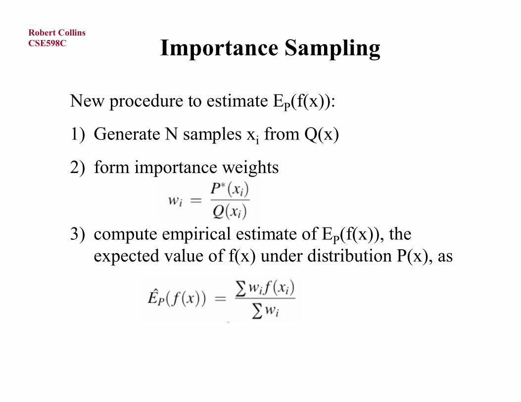
Importance Sampling

New procedure to estimate EP(f(x)):

1) Generate N samples xi from Q(x)

2) form importance weights

3) compute empirical estimate of EP(f(x)), the expected value of f(x) under distribution P(x), as


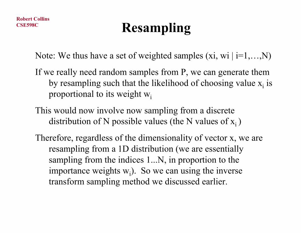
Resampling

Note: We thus have a set of weighted samples (xi, wi | i=1,…,N)

If we really need random samples from P, we can generate them by resampling such that the likelihood of choosing value xi is proportional to its weight wi

This would now involve now sampling from a discrete distribution of N possible values (the N values of xi )

Therefore, regardless of the dimensionality of vector x, we are resampling from a 1D distribution (we are essentially sampling from the indices 1...N, in proportion to the importance weights wi). So we can using the inverse transform sampling method we discussed earlier.


Note on Proposal Functions

Computational efficiency is best if the proposal distribution looks a lot like the desired distribution (area between curves is small).

These methods can fail badly when the proposal distribution has 0 density in a region where the desired distribution has non-negligeable density.

For this last reason, it is said that the proposal distribution should have heavy tails.


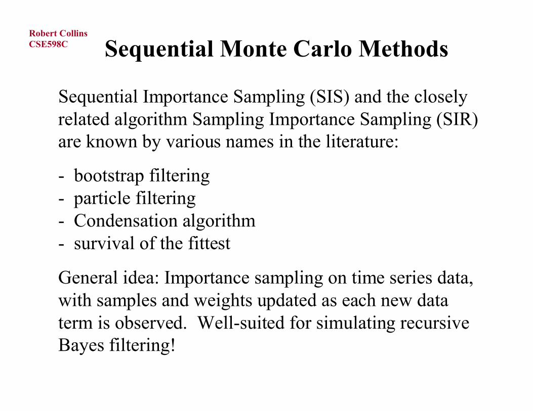
Sequential Monte Carlo Methods

Sequential Importance Sampling (SIS) and the closely related algorithm Sampling Importance Sampling (SIR) are known by various names in the literature:

- bootstrap filtering- particle filtering- Condensation algorithm- survival of the fittest

General idea: Importance sampling on time series data, with samples and weights updated as each new data term is observed. Well-suited for simulating recursive Bayes filtering!


Sequential Monte Carlo Methods

Intuition: each particle is a “guess” at the true state. For each one, simulate it’s motion update and add noise to get a motion prediction. Measure the likelihood of this prediction, and weight the resulting particles proportional to their likelihoods.


Back to Bayes Filtering

remember our intractible integrals:





This integral in the denominator of Bayes rule goes away for free, as a consequence of representing distributions by a weighted setof samples. Since we have only a finite number of samples, we can easily compute the normalization constant by summing the weights!




Now let’s write the Bayes filter by combining motion prediction and data correction steps into one equation.

motion term old posteriordata termnew posterior


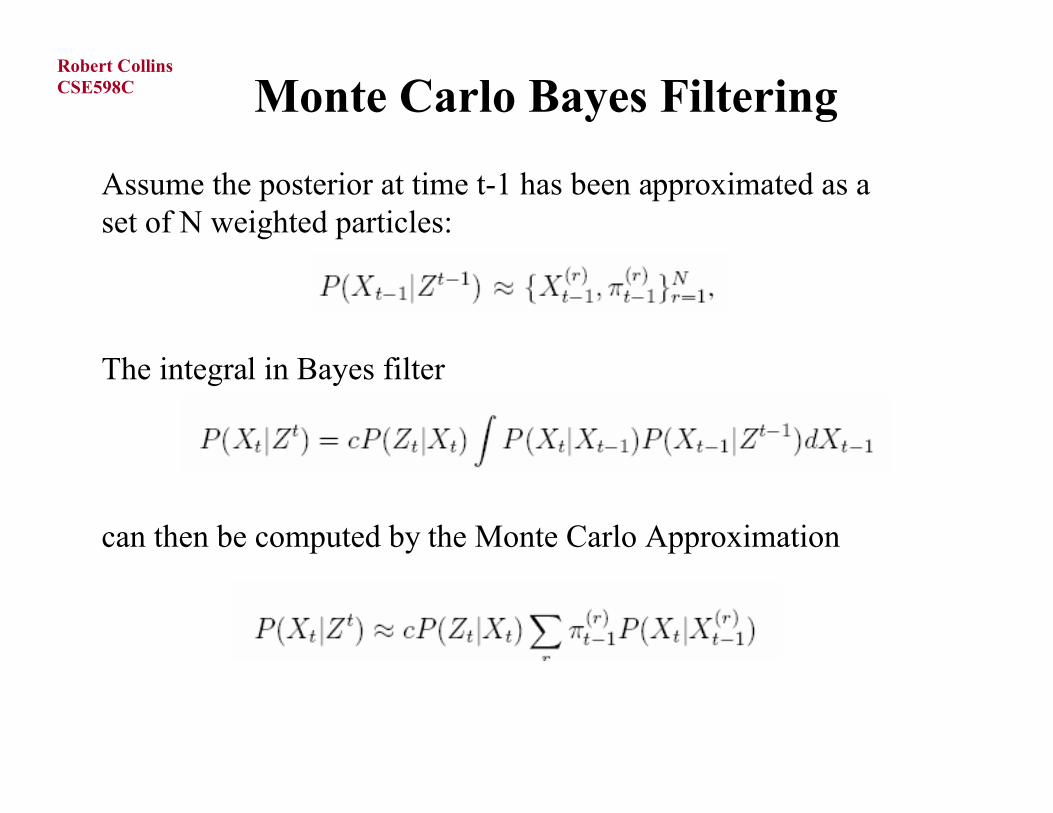
Monte Carlo Bayes Filtering

Assume the posterior at time t-1 has been approximated as a set of N weighted particles:

The integral in Bayes filter

can then be computed by the Monte Carlo Approximation


Representing the New Posterior

We can do this by importance sampling, where we draw samples from a proposal distribution q(Xt) that is a mixture density

To get a new weighted set of samples approximating the posterior at time t

Now let’s say we want to draw samples from this new posterior

The importance weights are computed as

P*Q

= =


Note

• the previous interpretation based on importance sampling from a mixture model is nonstandard, and due to Frank Dellaert.

• A more traditional interpretation can be found in the Arulampalam tutorial paper.


SIS Algorithm

SIR is then derived as a special case of SIS where1) importance density is the prior density2) resampling is done at every time step so that

all the sample weights are 1/N.


SIR Algorithm


Drawing from the Prior Density

xk = fk (xk-1, vk-1) v is process noise

note, when we use the prior as the importance density, we only need to sample from the process noise distribution (typically uniform or Gaussian).

Why? Recall:

Thus we can sample from the prior P(xk | xk-1) by generating a sample xi

k-1, generating a noise vector vik-1 from the noise process,

and forming the noisy sample

xik = fk (xi

k-1, vik-1)

If the noise is additive, this leads to a very simple interpretation: move each particle using motion prediction, then add noise.


Condensation (Isard&Blake)

time t-1

draw samples and apply motion predict

add noise (diffusion)

weight each sample by the likelihood

renormalize to get new set of samples

normalized set of weighted samples

time t


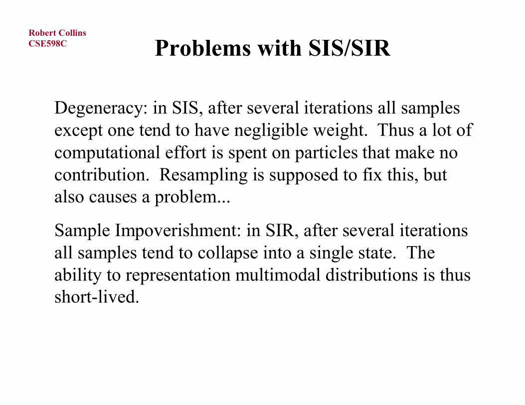
Problems with SIS/SIR

Degeneracy: in SIS, after several iterations all samples except one tend to have negligible weight. Thus a lot of computational effort is spent on particles that make no contribution. Resampling is supposed to fix this, but also causes a problem...

Sample Impoverishment: in SIR, after several iterations all samples tend to collapse into a single state. The ability to representation multimodal distributions is thus short-lived.


Next Time

We will look at the SIR sample impoverishment problem in detail, by viewing the algorithm’s behavior as a Markov Chain.

This is fruitful for two reasons.

1) understanding the limitations of SIR/Condensation

2) introduce ideas that form the basis of Markov Chain Monte Carlo (MCMC), which solves these problems.

sampling methods, particle filtering, and markov-chain monte carlo

Documents