markov chain monte carlo and applications
TRANSCRIPT

Dean Lee Facility for Rare Isotope Beams Michigan State University Nuclear Lattice EFT Collaboration Bayesian Inference in Subatomic Physics – A Wallenberg Symposium Gothenburg, Sept. 17, 2019
1
Markov Chain Monte Carlo and Applications

Outline
Markov chain Monte Carlo
Lattice effective field theory
Eigenvector continuation
Eigenvector continuation as an emulator
Summary
2

Oxygen-16
3
Animation by Gabriel Given lattice spacing = 1.32 fm

We will be discussing Markov chain algorithms, and so it is useful to review the elements and theory of Markov chains. Consider a chain of configurations labeled by order of selection. We call this integer-valued label the computation step.
Let us denote the probability of selecting configuration A at computation step n as
Suppose we have selected configuration A at computation step n. The probability that we select configuration B at computation step n + 1 is denoted
4
Markov chain Monte Carlo

This transition probability is chosen to be independent of n and independent of the history of configurations selected prior to selecting A at computation step n. This defines a Markov chain.
We note that
5
We now define the notion of ergodicity. Suppose we are at configuration A at computation step, n. Let SA be the set of all positive integers m, such that the return probability to A is nonzero
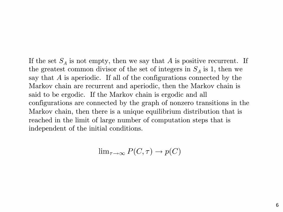
If the set SA is not empty, then we say that A is positive recurrent. If the greatest common divisor of the set of integers in SA is 1, then we say that A is aperiodic. If all of the configurations connected by the Markov chain are recurrent and aperiodic, then the Markov chain is said to be ergodic. If the Markov chain is ergodic and all configurations are connected by the graph of nonzero transitions in the Markov chain, then there is a unique equilibrium distribution that is reached in the limit of large number of computation steps that is independent of the initial conditions.
6

Detailed balance
We want the equilibrium probability distribution to be
One way to do this is to require
for every pair of configurations A and B. This condition is called detailed balance.
7
If the Markov chain is ergodic and all configurations are connected, then after many computation steps we reach the unique equilibrium distribution, which satisfies the stationary condition

for all configurations A.
Comparing with the detailed balance condition, we conclude that
8
One popular method for generating the desired detailed balance condition is the Metropolis algorithm Metropolis, Teller, Rosenbluth, J. Chem. Phys. 21 (1953) 1087
Metropolis algorithm

Usually the transition probability can be divided in terms of a proposed move probability and an acceptance probability,
In the original Metropolis algorithm the proposed move probability is symmetric
The more general case where the proposed move can be asymmetric is the Metropolis-Hastings algorithm. It is also not necessary that you use only one type of update. If you maintain detailed balance for each type of update process and and ergodicity, then you recover the target probability distribution.
9

Another algorithm that yields detail balance is the heat bath algorithm where
Heat bath algorithm
The heat bath algorithm can be generalized to allow for a large family of possible transitions
Gibbs sampling
Gibbs sampling is the heat bath algorithm applied to updates of a single degree of freedom in the system.
10

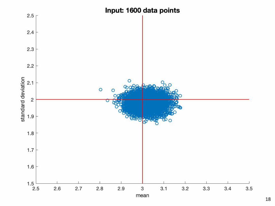
Let the data D = {xi} be N data points selected from a normal distribution with mean 3.00 and standard deviation 2.00. We use a simple model of the data of the form
We start from no previous data, and set the prior P (a, b) equal to a constant.
The posterior probability is
11
Example

In that case we can write
A sample code to perform Markov Chain Monte Carlo sampling of the posterior distribution is given on the next page.


14

15

16

17
18
n
n
p
p
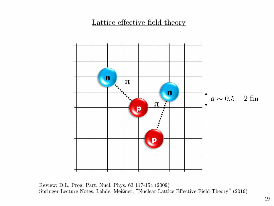
Lattice effective field theory
π
π
Review: D.L, Prog. Part. Nucl. Phys. 63 117-154 (2009) Springer Lecture Notes: Lähde, Meißner, “Nuclear Lattice Effective Field Theory” (2019)
19

Construct the effective potential order by order
20
N
N
N
N
π
N
N
N
N
N
N
N
N
ππ
N
N
N
N
Contact interactions
Leading order (LO) Next-to-leading order (NLO)
Chiral effective field theory

π
π
21
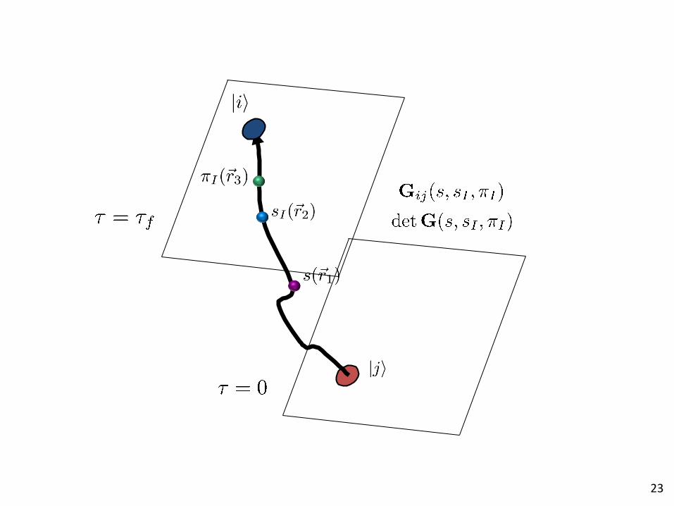
Euclidean time projection

We can write exponentials of the interaction using a Gaussian integral identity
We remove the interaction between nucleons and replace it with the interactions of each nucleon with a background field.
22
Auxiliary field method
23

0 10 20 30 40 50
-400
-300
-200
-100
0
CaArS
Si
Mg
Ne
O
C
BeHe
Lattice Exp.
Bin
ding
ene
rgy
(MeV
)
Mass number A
H Pion-less EFT Leading Order
24Lu, Li, Elhatisari, D.L., Epelbaum, Meißner, PLB 797, 134863 (2019)

Pinhole Algorithm
Consider the density operator for nucleon with spin i and isospin j
We construct the normal-ordered A-body density operator
In the simulations we do Monte Carlo sampling of the amplitude
25

i1,j1
i2,j2
i3,j3
i4,j4 i5,j5
i6,j6
i7,j7
i9,j9 i10,j10
i11,j11
i15,j15
Metropolis Monte Carlo updates of pinholes
Hybrid Monte Carlo updates of auxiliary/pion fields
i13,j13
i12,j12
i14,j14
i16,j16
i8,j8
Elhatisari, Epelbaum, Krebs, Lähde, D.L., Li, Lu, Meißner, Rupak, PRL 119, 222505 (2017)
26

Oxygen-16
27
Animation by Gabriel Given lattice spacing = 1.32 fm

We demonstrate that when a control parameter in the Hamiltonian matrix is varied smoothly, the extremal eigenvectors do not explore the large dimensionality of the linear space. Instead they trace out trajectories with significant displacements in only a small number of linearly-independent directions.
Eigenvector continuation
We can prove this empirical observation using analytic function theory and the principles of analytic continuation.
Since the eigenvector trajectory is a low-dimensional manifold embedded in a very large space, we can find the desired eigenvector using a variational subspace approximation.
28
D. Frame, R. He, I. Ipsen, Da. Lee, De. Lee, E. Rrapaj, PRL 121 (2018) 032501
29
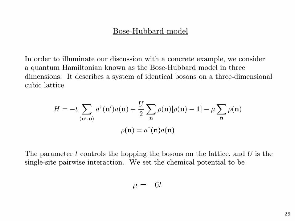
Bose-Hubbard model
In order to illuminate our discussion with a concrete example, we consider a quantum Hamiltonian known as the Bose-Hubbard model in three dimensions. It describes a system of identical bosons on a three-dimensional cubic lattice.
The parameter t controls the hopping the bosons on the lattice, and U is the single-site pairwise interaction. We set the chemical potential to be
-10
-8
-6
-4
-2
0
2
4
6
-5 -4 -3 -2 -1 0 1 2
E 0/t
U/t
exact energiesperturbation order 1perturbation order 2perturbation order 3perturbation order 4perturbation order 5perturbation order 6
30
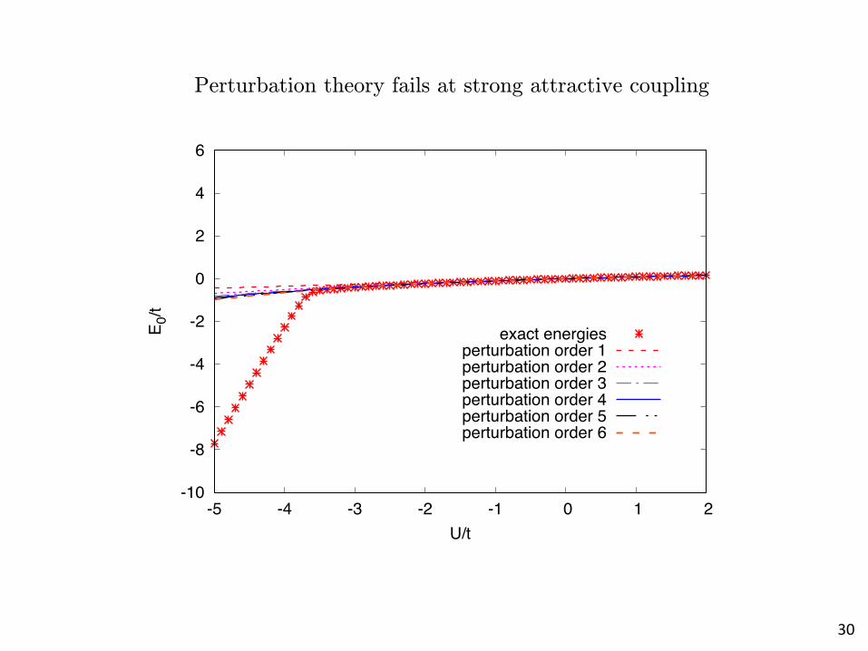
Perturbation theory fails at strong attractive coupling

-10
-8
-6
-4
-2
0
2
4
6
-5 -4 -3 -2 -1 0 1 2
E 0/t
U/t
exact energiesEC with 3 sampling points
sampling points
31
Restrict the linear space to the span of three vectors
-10
-8
-6
-4
-2
0
2
4
6
-5 -4 -3 -2 -1 0 1 2
E 0/t
U/t
exact energiesEC with 1 sampling point
EC with 2 sampling pointsEC with 3 sampling pointsEC with 4 sampling pointsEC with 5 sampling points
sampling points
32
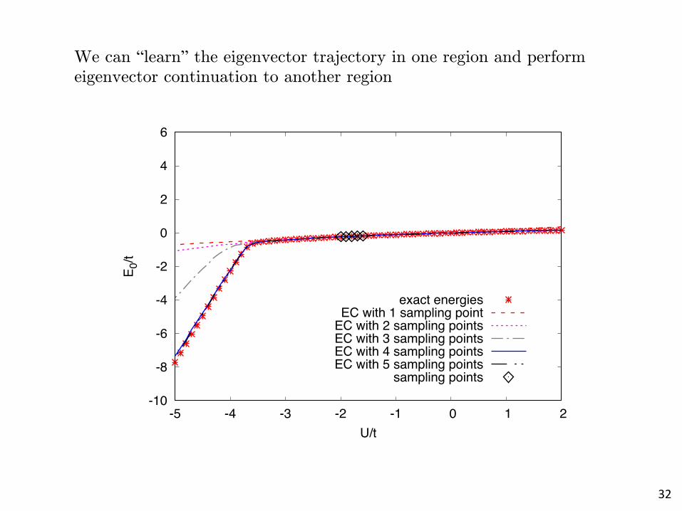
We can “learn” the eigenvector trajectory in one region and perform eigenvector continuation to another region
-10
-8
-6
-4
-2
0
2
4
6
-5 -4 -3 -2 -1 0 1 2
E/t
U/t
exact energiesEC with 1 sampling point
EC with 2 sampling pointsEC with 3 sampling pointsEC with 4 sampling pointsEC with 5 sampling points
sampling points
33
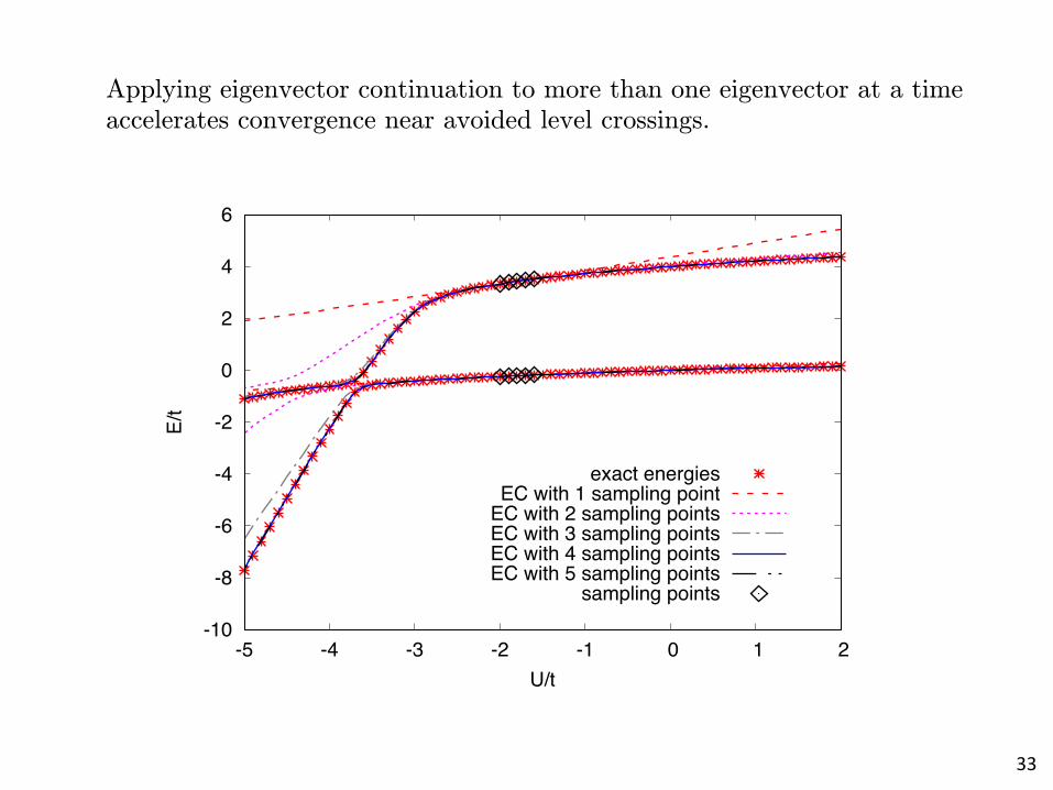
Applying eigenvector continuation to more than one eigenvector at a time accelerates convergence near avoided level crossings.
34
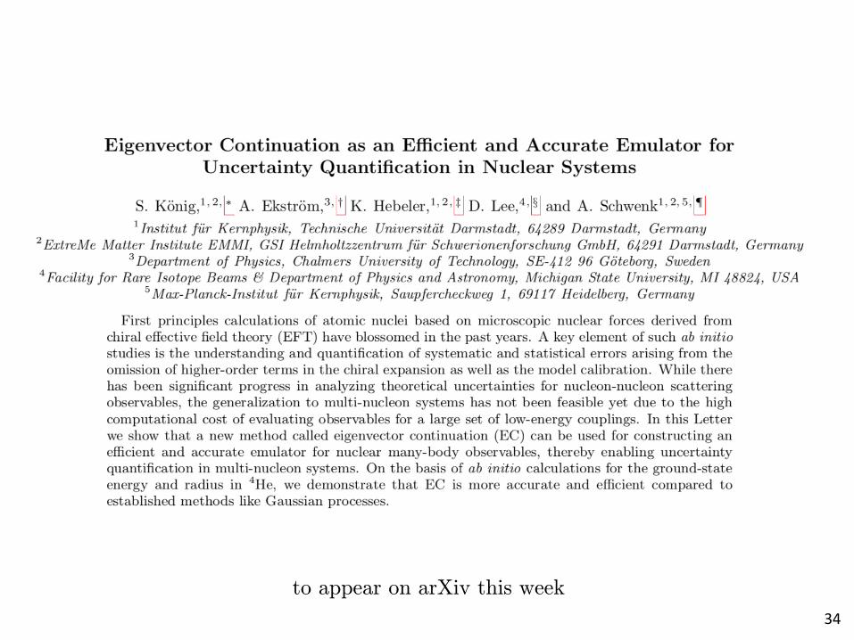
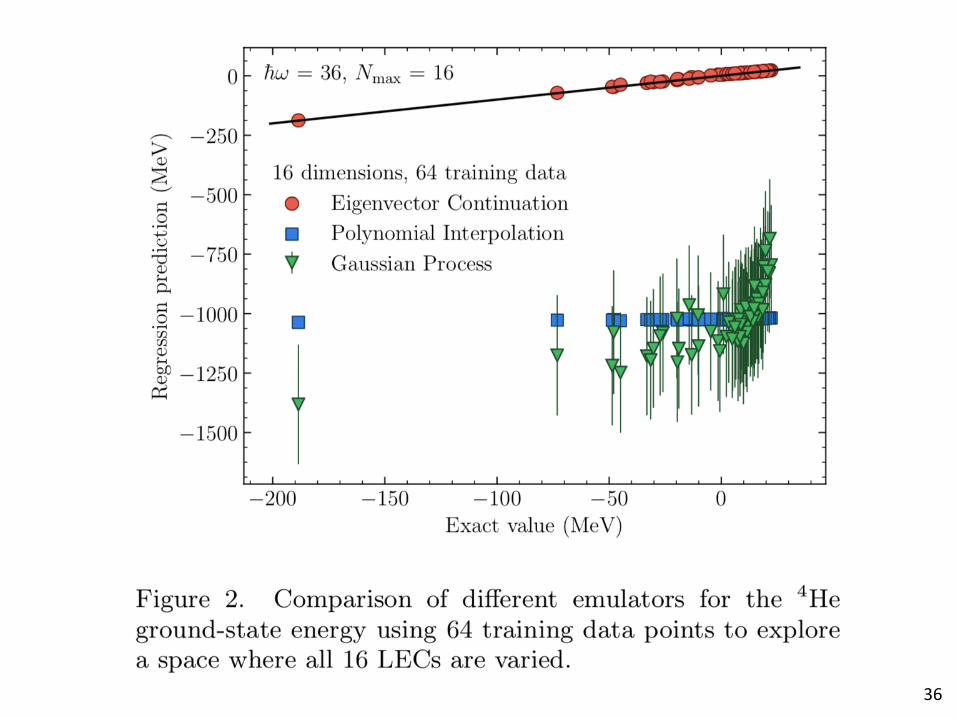
to appear on arXiv this week

35
36

37

Summary
Markov chain Monte Carlo is a powerful and flexible tool that can be used to sample probability distributions. In particular, it can be used with Bayesian inference to determine posterior probabilities.
Lattice effective field theory is a first principles method that combines lattice methods and effective field theory. It is being for calculations of nuclear structure and reactions.
38
Eigenvector continuation is based on the observation that an eigenvector varies smoothly on the parameters of the matrix. As a result, they can be well-described by a low-dimensional manifold and approximated using a small variational subspace. This can be used as a fast and accurate emulator for quantum systems.
39