Introduction to RooFit

1. Introduction and overview

2. Creation and basic use of models

3. Addition and Convolution

4. Common Fitting Problems

W. Verkerke (NIKHEF)

4. Common Fitting Problems

5. Multidimensional and Conditional models

6. Fit validation and toy MC studies

7. Constructing joint model

8. Working with the Likelihood, including systematic errors

9. Interval & Limits

Introduction & Overview1 & Overview1

Introduction -- Focus: coding a probability density function

• Focus on one practical aspect of many data analysis in HEP: How do you formulate your p.d.f. in ROOT– For ‘simple’ problems (gauss, polynomial) this is easy

1

– But if you want to do unbinned ML fits, use non-trivial functions, or work with multidimensional functions you quickly find that you need some tools to help you

Introduction – Why RooFit was developed

• BaBar experiment at SLAC: Extract sin(2β) from time dependent CP violation of B decay: e+e- à Y(4s) à BB– Reconstruct both Bs, measure decay time difference

– Physics of interest is in decay time dependent oscillation

( )[ ]( )[ ]);|BkgResol();(BkgDecay);BkgSel()1(

);|SigResol())2sin(,;(SigDecay);SigSel( sigsigsigsig

rdttqtpmf

rdttqtpmfrr

rr

⊗⋅−

+⊗⋅⋅ β

2

• Many issues arise– Standard ROOT function framework clearly insufficient to handle such

complicated functions à must develop new framework

– Normalization of p.d.f. not always trivial to calculate à may need numeric integration techniques

– Unbinned fit, >2 dimensions, many events à computation performance important à must try optimize code for acceptable performance

– Simultaneous fit to control samples to account for detector performance

( )[ ]);|BkgResol();(BkgDecay);BkgSel()1( bkgbkgbkgsig rdttqtpmfrr

⊗⋅−

Mathematic – Probability density functions

• Probability Density Functions describe probabilities, thus– All values most be >0

– The total probability must be 1 for each p, i.e.

– Can have any number of dimensions 1),(max

min

≡∫x

x

xdpxg

v

v

vvv

Wouter Verkerke, NIKHEF

• Note distinction in role between parameters (p) and observables (x)– Observables are measured quantities

– Parameters are degrees of freedom in your model

∫ ≡1)( dxxF ∫ ≡1),( dxdyyxF

Math – Functions vs probability density functions

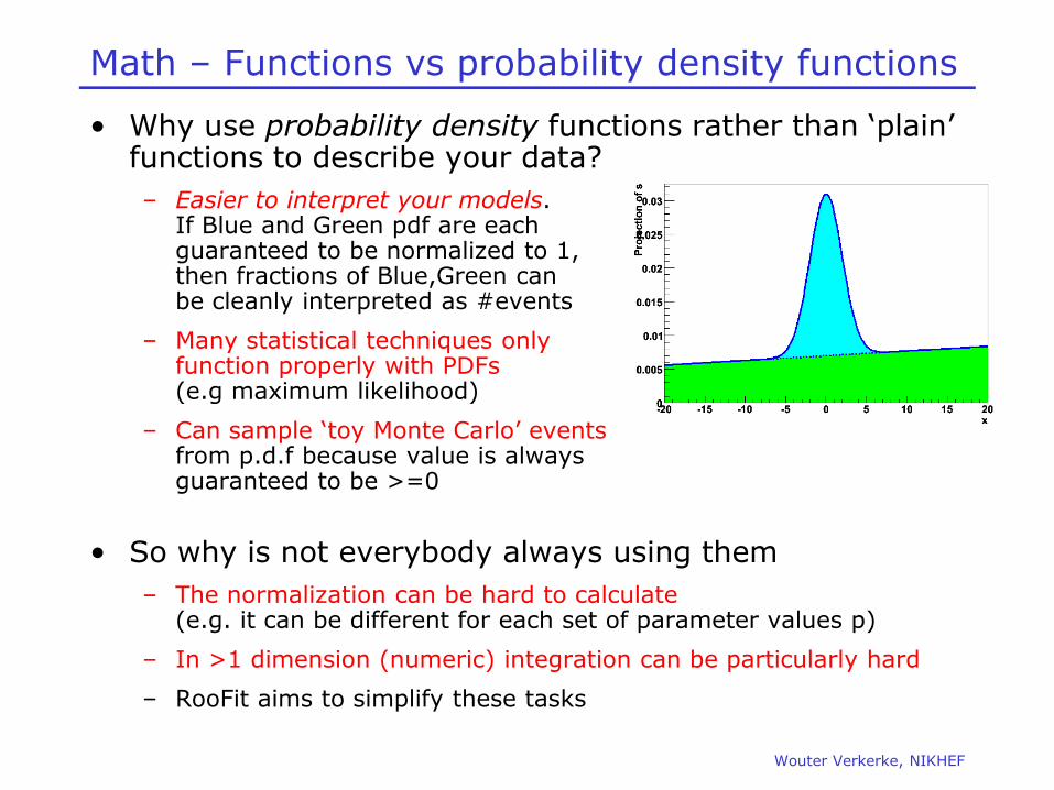
• Why use probability density functions rather than ‘plain’ functions to describe your data?– Easier to interpret your models.

If Blue and Green pdf are each guaranteed to be normalized to 1, then fractions of Blue,Green can be cleanly interpreted as #events

– Many statistical techniques onlyfunction properly with PDFs(e.g maximum likelihood)

Wouter Verkerke, NIKHEF

(e.g maximum likelihood)

– Can sample ‘toy Monte Carlo’ eventsfrom p.d.f because value is always guaranteed to be >=0

• So why is not everybody always using them– The normalization can be hard to calculate

(e.g. it can be different for each set of parameter values p)

– In >1 dimension (numeric) integration can be particularly hard

– RooFit aims to simplify these tasks

Introduction – Relation to ROOT

ToyMC data Data/Model

Data Modeling

Model

Extension to ROOT – (Almost) no overlap with existing functionality

3

C++ command line interface & macros

Data management &histogramming

Graphics interface

I/O support

MINUIT

ToyMC dataGeneration

Data/ModelFitting

Model Visualization

Project timeline

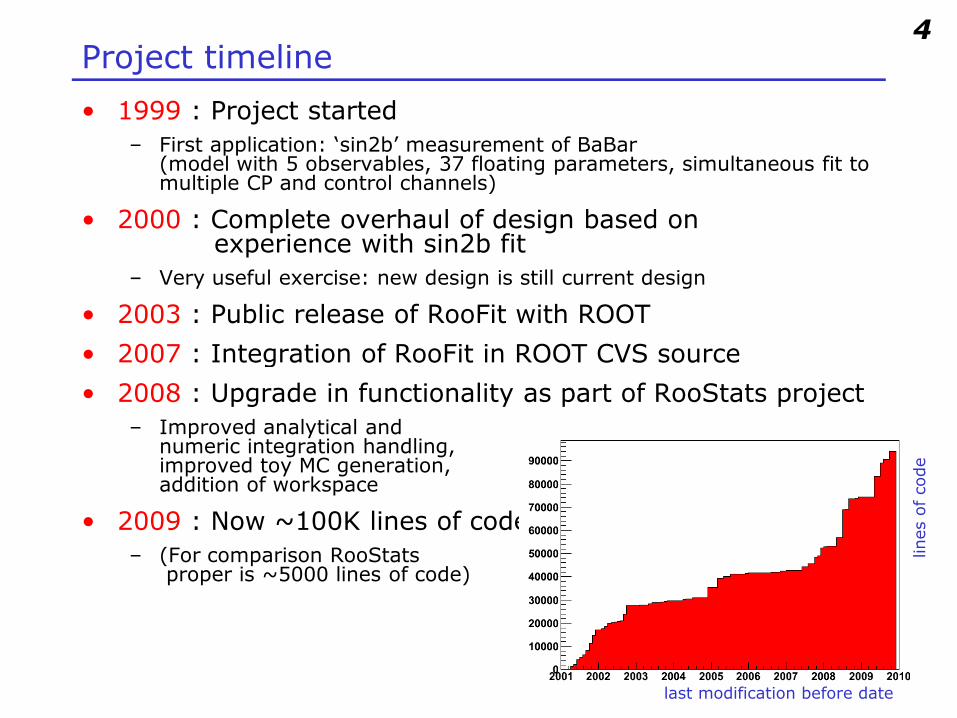
• 1999 : Project started– First application: ‘sin2b’ measurement of BaBar

(model with 5 observables, 37 floating parameters, simultaneous fit to multiple CP and control channels)

• 2000 : Complete overhaul of design based on experience with sin2b fit

– Very useful exercise: new design is still current design

• 2003 : Public release of RooFit with ROOT

• 2007 : Integration of RooFit in ROOT CVS source

4

• 2007 : Integration of RooFit in ROOT CVS source

• 2008 : Upgrade in functionality as part of RooStats project– Improved analytical and

numeric integration handling, improved toy MC generation, addition of workspace

• 2009 : Now ~100K lines of code – (For comparison RooStats

proper is ~5000 lines of code)

last modification before date

lines

of co

de

RooFit core design philosophy

• Mathematical objects are represented as C++ objects

variable RooRealVar

function RooAbsReal

RooFit classMathematical concept

x)(xf

5

PDF RooAbsPdf

space point RooArgSet

list of space points RooAbsData

integral RooRealIntegral

)(xfxr

dxxfx

x∫max

min

)(

RooFit core design philosophy

• Represent relations between variables and functionsas client/server links between objects

f(x,y,z)

RooAbsReal f

Math

6

RooRealVar x RooRealVar y RooRealVar z

RooRealVar x(“x”,”x”,5) ;RooRealVar y(“y”,”y”,5) ;RooRealVar z(“z”,”z”,5) ;RooBogusFunction f(“f”,”f”,x,y,z) ;

RooFitdiagram

RooFitcode

Basic use22

The simplest possible example

• We make a Gaussian p.d.f. with three variables: mass, mean and sigma

RooRealVar x(“x”,”Observable”,-10,10) ;

RooRealVar mean(“mean”,”B0 mass”,0.00027,”GeV”);

RooRealVar sigma(“sigma”,”B0 mass width”,5.2794,”GeV”) ;

Objects representinga ‘real’ value.

Initial range

Name of object Title of object

RooRealVar sigma(“sigma”,”B0 mass width”,5.2794,”GeV”) ;

RooGaussian model(“model”,”signal pdf”,mass,mean,sigma)PDF object

Initial value Optional unit

References to variables

Basics – Creating and plotting a Gaussian p.d.f

// Create an empty plot frameRooPlot* xframe = w::x.frame() ;

// Plot model on framemodel.plotOn(xframe) ;

// Draw frame on canvasxframe->Draw() ;

Setup gaussian PDF and plot

13

Plot range taken from limits of x

Axis label from gauss title

Unit normalizationA RooPlot is an empty frame

capable of holding anythingplotted versus it variable

Basics – Generating toy MC events

// Generate an unbinned toy MC setRooDataSet* data = w::gauss.generate(w::x,10000) ;

// Generate an binned toy MC setRooDataHist* data = w::gauss.generateBinned(w::x,10000) ;

// Plot PDFRooPlot* xframe = w::x.frame() ;

Generate 10000 events from Gaussian p.d.f and show distribution

14

RooPlot* xframe = w::x.frame() ;data->plotOn(xframe) ;xframe->Draw() ;

Can generate both binned andunbinned datasets

Basics – Importing data

• Unbinned data can also be imported from ROOT TTrees

– Imports TTree branch named “x”.

– Can be of type Double_t, Float_t, Int_t or UInt_t. All data is converted to Double_t internally

– Specify a RooArgSet of multiple observables to import

// Import unbinned dataRooDataSet data(“data”,”data”,w::x,Import(*myTree)) ;

15

– Specify a RooArgSet of multiple observables to importmultiple observables

• Binned data can be imported from ROOT THx histograms

– Imports values, binning definition and SumW2 errors (if defined)

– Specify a RooArgList of observables when importing a TH2/3.

// Import unbinned dataRooDataHist data(“data”,”data”,w::x,Import(*myTH1)) ;

Basics – ML fit of p.d.f to unbinned data

// ML fit of gauss to dataw::gauss.fitTo(*data) ;(MINUIT printout omitted)

// Parameters if gauss now

PDFautomaticallynormalizedto dataset

16

// Parameters if gauss now// reflect fitted valuesw::mean.Print()RooRealVar::mean = 0.0172335 +/- 0.0299542 w::sigma.Print()RooRealVar::sigma = 2.98094 +/- 0.0217306

// Plot fitted PDF and toy data overlaidRooPlot* xframe = w::x.frame() ;data->plotOn(xframe) ;w::gauss.plotOn(xframe) ;

to dataset

Basics – ML fit of p.d.f to unbinned data

• Can also choose to save full detail of fit

RooFitResult* r = w::gauss.fitTo(*data,Save()) ;

r->Print() ;RooFitResult: minimized FCN value: 25055.6,

estimated distance to minimum: 7.27598e-08coviarance matrix quality: Full, accurate covariance matrix

Floating Parameter FinalValue +/- Error

17

Floating Parameter FinalValue +/- Error -------------------- --------------------------

mean 1.7233e-02 +/- 3.00e-02sigma 2.9809e+00 +/- 2.17e-02

r->correlationMatrix().Print() ;

2x2 matrix is as follows

| 0 | 1 |-------------------------------

0 | 1 0.0005869 1 | 0.0005869 1

Organizing your analysis project – Factory and workspace

• When moving beyond simple Gaussian example, some need to organize analysis project.– RooFit provides 2 standard tools to help

• Workspace– A generic container class for all RooFit objects of your project

– Fill with import() from top-level pdf. Automatically imports all components and variables

RooWorkspace w(“w”) ; w.import(model) ;w.Print() ;

variables---------(mean,sigma,x)

p.d.f.s-------RooGaussian::f[ x=x mean=mean sigma=sigma ] = 0.249352

Organizing your analysis project – Factory and workspace

• Advantages of organizing code with the workspace– Allows to create and use models in separate places

– Allows to share models easily between ROOT sessions and users:Workspace objects are persistable in ROOT files(*)

• Access contents either through accessor methods

RooPlot* frame = w.var(“x”)->frame() ;

• Or through CINT namespace (interactive ROOT only)

– Must first call w.exportToCint() or create workspace with kTRUEas 2nd argument

w.pdf(“g”)->plotOn(frame) ;

RooPlot* frame = w::x.frame() ;w::g.plotOn(frame) ;

(*) Full support for a B physics pdfs by end of year

Factory and Workspace

• One C++ object per math symbol provides ultimate level of control over each objects functionality, but results in lengthy user code for even simple macros

• Solution: add factory that auto-generates objects from a math-like language

8

Gaussian::f(x[-10,10],mean[5],sigma[3])

RooRealVar x(“x”,”x”,-10,10) ;RooRealVar mean(“mean”,”mean”,5) ;RooRealVar sigma(“sigma”,”sigma”,3) ;RooGaussian f(“f”,”f”,x,mean,sigma) ;

Factory and Workspace

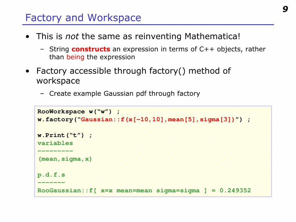
• This is not the same as reinventing Mathematica!– String constructs an expression in terms of C++ objects, rather

than being the expression

• Factory accessible through factory() method of workspace– Create example Gaussian pdf through factory

RooWorkspace w(“w”) ;

9

RooWorkspace w(“w”) ;w.factory(“Gaussian::f(x[-10,10],mean[5],sigma[3])”) ;

w.Print(“t”) ;variables---------(mean,sigma,x)

p.d.f.s-------RooGaussian::f[ x=x mean=mean sigma=sigma ] = 0.249352

Factory language

• The factory language has a 1-to-1 mapping to the constructor syntax of RooFit classes– With a few handy shortcuts for variables

• Creating variables

x[-10,10] // Create variable with given range, init val is midpointx[5,-10,10] // Create variable with initial value and range

11

• Creating pdfs (and functions)

– Can always omit leading ‘Roo’

– Curly brackets translate to set or list argument (depending on context)

x[5] // Create initially constant variable

Gaussian::g(x,mean,sigma) àààà RooGaussian(“g”,”g”,x,mean,sigma)Polynomial::p(x,{a0,a1}) àààà RooPolynomial(“p”,”p”,x”,RooArgList(a0,a1));

Factory language

• Composite expression are created by nesting statements– No limit to recursive nesting

Gaussian::g(x[-10,10],mean[-10,10],sigma[3]) àààà x[-10,10]

mean[-10,10]sigma[3]Gaussian::g(x,mean,sigma)

12

• You can also use numeric constants whenever an unnamed constant is needed

• Names of nested function objects are optional• SUM syntax explained later

Gaussian::g(x[-10,10],0,3)

SUM::model(0.5*Gaussian(x[-10,10],0,3),Uniform(x)) ;

Model building – (Re)using standard components

• RooFit provides a collection of compiled standard PDF classes

RooArgusBG

RooPolynomial

RooBMixDecay

RooHistPdf

Physics inspiredARGUS,Crystal Ball, Breit-Wigner, Voigtian,B/D-Decay,….

Non-parametricHistogram, KEYS

20

RooGaussian

BasicGaussian, Exponential, Polynomial,…Chebychev polynomial

Histogram, KEYS

Easy to extend the library: each p.d.f. is a separate C++ class

Model building – (Re)using standard components

• List of most frequently used pdfs and their factory spec

Gaussian Gaussian::g(x,mean,sigma)

Breit-Wigner BreitWigner::bw(x,mean,gamma)

Landau Landau::l(x,mean,sigma)

Exponential Exponental::e(x,alpha)

21

Polynomial Polynomial::p(x,{a0,a1,a2})

Chebychev Chebychev::p(x,{a0,a1,a2})

Kernel Estimation KeysPdf::k(x,dataSet)

Poisson Poisson::p(x,mu)

Voigtian Voigtian::v(x,mean,gamma,sigma)(=BW⊗G)

Model building – Making your own

• Interpreted expressions

• Customized class, compiled and linked on the fly

w.factory(“EXPR::mypdf(‘sqrt(a*x)+b’,x,a,b)”) ;

22

• Custom class written by you– Offer option of providing analytical integrals, custom handling of

toy MC generation (details in RooFit Manual)

• Compiled classes are faster in use, but require O(1-2) seconds startup overhead– Best choice depends on use context

w.factory(“CEXPR::mypdf(‘sqrt(a*x)+b’,x,a,b)”) ;

Model building – Adjusting parameterization

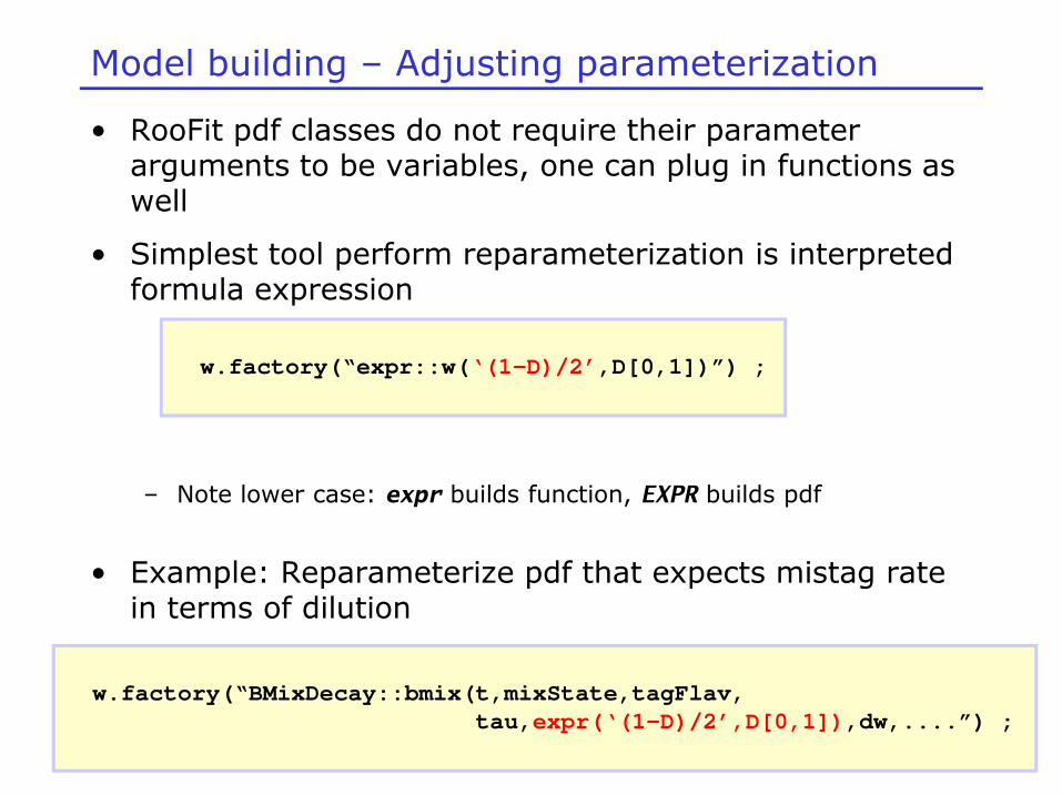
• RooFit pdf classes do not require their parameter arguments to be variables, one can plug in functions as well

• Simplest tool perform reparameterization is interpreted formula expression

w.factory(“expr::w(‘(1-D)/2’,D[0,1])”) ;

– Note lower case: expr builds function, EXPR builds pdf

• Example: Reparameterize pdf that expects mistag rate in terms of dilution

w.factory(“BMixDecay::bmix(t,mixState,tagFlav,tau,expr(‘(1-D)/2’,D[0,1]),dw,....”) ;

Composite models3 models3

RooBMixDecay

RooPolynomial

RooHistPdf

RooArgusBG

Model building – (Re)using standard components

• Most realistic models are constructed as the sum of one or more p.d.f.s (e.g. signal and background)

• Facilitated through operator p.d.f RooAddPdf

23

RooArgusBG

RooAddPdf+

RooGaussian

Adding p.d.f.s – Mathematical side

• From math point of view adding p.d.f is simple– Two components F, G

– Generically for N components P0-PN

)()1()()( xGfxfFxS −+=

)(1)(...)()()( 111100 xPcxPcxPcxPcxS ninn

−++++= ∑

−=−−

24

• For N p.d.f.s, there are N-1 fraction coefficients that should sum to less 1– The remainder is by construction 1 minus the sum of all other

coefficients

1,0 ni

∑−=

Adding p.d.f.s – Factory syntax

• Additions created through a SUM expression

– Note that last PDF does not have an associated fraction

SUM::name(frac1*PDF1,frac2*PDF2,...,PDFN)

25

• Complete example

w.factory(“Gaussian::gauss1(x[0,10],mean1[2],sigma[1]”) ;w.factory(“Gaussian::gauss2(x,mean2[3],sigma)”) ;w.factory(“ArgusBG::argus(x,k[-1],9.0)”) ;

w.factory(“SUM::sum(g1frac[0.5]*gauss1, g2frac[0.1]*gauss2, argus)”)

Extended ML fits

• In an extended ML fit, an extra term is added to the likelihood

Poisson(Nobs,Nexp)

• This is most useful in combination with a composite pdf

NNxBfxSfxF =−+⋅= exp;)()1()()(

27

shape normalization

BSBS

B

BS

S NNNxBNN

NxS

NNN

xF +=+

+⋅+

= exp;)()()(

BS NNNf ,, ⇒

SUM::name(Nsig*S,Nbkg*B)

Write like this, extended term automatically included in –log(L)

Component plotting - Introduction

• Plotting, toy event generation and fitting works identically for composite p.d.f.s– Several optimizations applied

behind the scenes that are specific to composite models (e.g. delegate event generation to components)

• Extra plotting functionality

26

• Extra plotting functionality specific to composite pdfs– Component plotting

// Plot only argus componentsw::sum.plotOn(frame,Components(“argus”),LineStyle(kDashed)) ;

// Wildcards allowedw::sum.plotOn(frame,Components(“gauss*”),LineStyle(kDashed)) ;

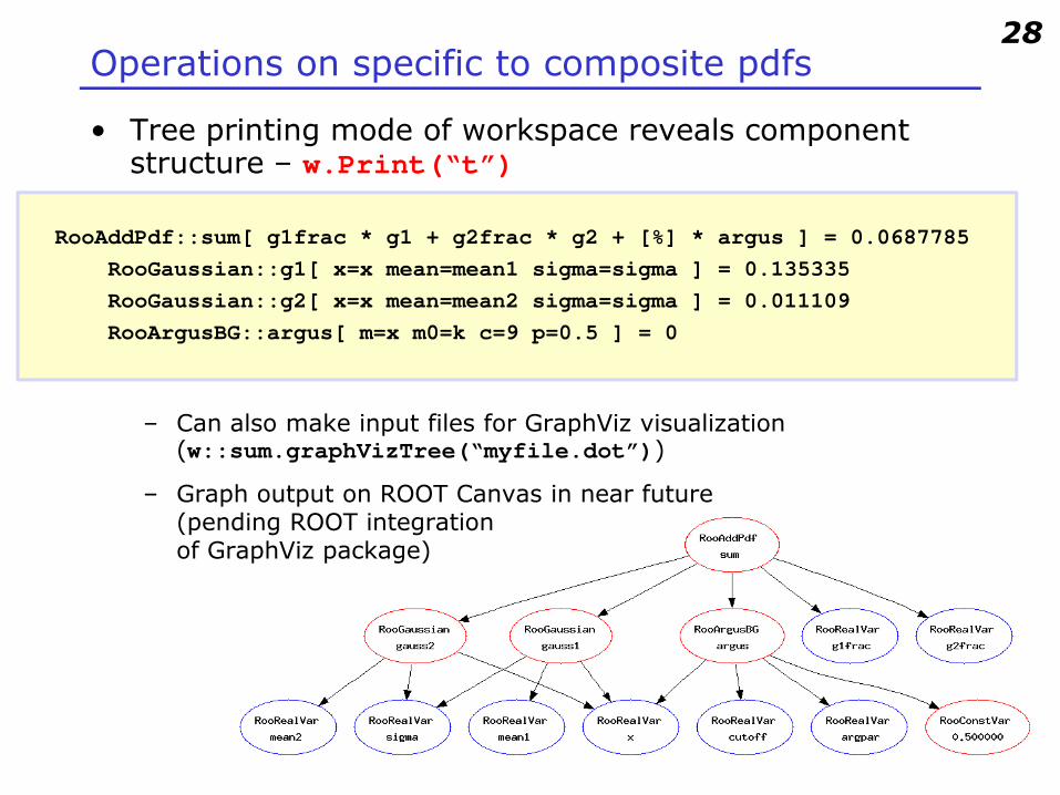
Operations on specific to composite pdfs

• Tree printing mode of workspace reveals component structure – w.Print(“t”)

RooAddPdf::sum[ g1frac * g1 + g2frac * g2 + [%] * argus ] = 0.0687785 RooGaussian::g1[ x=x mean=mean1 sigma=sigma ] = 0.135335RooGaussian::g2[ x=x mean=mean2 sigma=sigma ] = 0.011109RooArgusBG::argus[ m=x m0=k c=9 p=0.5 ] = 0

28

– Can also make input files for GraphViz visualization(w::sum.graphVizTree(“myfile.dot”))

– Graph output on ROOT Canvas in near future(pending ROOT integrationof GraphViz package)

Convolution

• Model representing a convolution of a theory model and a resolution model often useful

⊗⊗⊗⊗ =

∫+∞

∞−

′′−=⊗ xdxxgxfxgxf )()()()(

29

• But numeric calculation of convolution integral can bechallenging. No one-size-fits-all solution, but 3 options available– Analytical convolution (BW⊗Gauss, various B physics decays)

– Brute-force numeric calculation (slow)

– FFT numeric convolution (fast, but some side effects)

⊗⊗⊗⊗ =

Framework for analytical calculations of convolutions

• Convoluted PDFs that can be written if the following form can be used in a very modular way in RooFit

( )∑ ⊗=k

kk dtRdtfcdtP ,...)(,...)((...),...)(

‘basis function’coefficient

Wouter Verkerke, NIKHEF

‘basis function’coefficient

resolution function

)cos(),21(

,1/||

11

/||00

tmefwc

efwct

t

⋅∆=−±=

=∆±=−

−

τ

τExample: B0 decay with mixing

Analytical convolution

• Physics model and resolution model are implemented separately in RooFit

( )∑ ⊗= kk dtRdtfcdtP ,...)(,...)((...),...)(

RooResolutionModel

Implements Also a PDF by itself

,...)(,...)( dtRdtfi ⊗

Wouter Verkerke, NIKHEF

( )∑ ⊗=k

kk dtRdtfcdtP ,...)(,...)((...),...)(

RooAbsAnaConvPdf (physics model)

User can choose combination of physics model and resolution model at run time(Provided resolution model implements all fk declared by physics model)

Implements ckDeclares list of fk needed

Analytical convolution (for B physics decays)

• For most B meson decay time distribution (including effects of CPV and mixing) it is possible to calculate convolution analytically

• Example

w.factory(“GaussModel::gm(t[-10,10],0,1”)w.factory(“BMixDecay::bmix(t,mixState[mixed=-1,unmixed=1],

tagFlav[B0=1,B0bar=-1],tau[1.54],

• Other resolution models of interest

tagFlav[B0=1,B0bar=-1],tau[1.54],dm[0.472],w[0.2],dw[0],gm) ;

w.factory(“TruthModel::tm(t[-10,10])”) ; // Delta functionw.factory(“AddModel::am({gm1,gm2},f)”) ; // Sum of any N models

Examples

w.factory(“TruthModel::gm(t[-10,10]) ;w.factory(“Decay::bmix(t,tau[1.54],gm) ;

w.factory(“GaussModel::gm(t[-10,10],0,1”)w.factory(“GaussModel::gm(t[-10,10],0,1”)w.factory(“Decay::bmix(t,tau[1.54],gm) ;

w.factory(“AddModel::gm12({gm,GaussModel::gm2(t,0,5)},0.5)”) ;

w.factory(“Decay::bmix(t,tau[1.54],gm12);

Numeric Convolution

• Example

w.factory(“Landau::L(x[-10,30],5,1)”) :w.factory(“Gaussian::G(x,0,2)”) ;

w::x.setBins(“cache”,10000) ; // FFT sampling densityw.factory(“FCONV::LGf(x,L,G)”) ; // FFT convolution

w.factory(“NCONV::LGb(x,L,G)”) ; // Numeric convolution

30

• FFT usually best– Fast: unbinned ML fit to 10K

events take ~5 seconds

– NB: Requires installation of FFTWpackage (free, but not default)

– Beware of cyclical effects(some tools available to mitigate)

Exercises* Exercises*

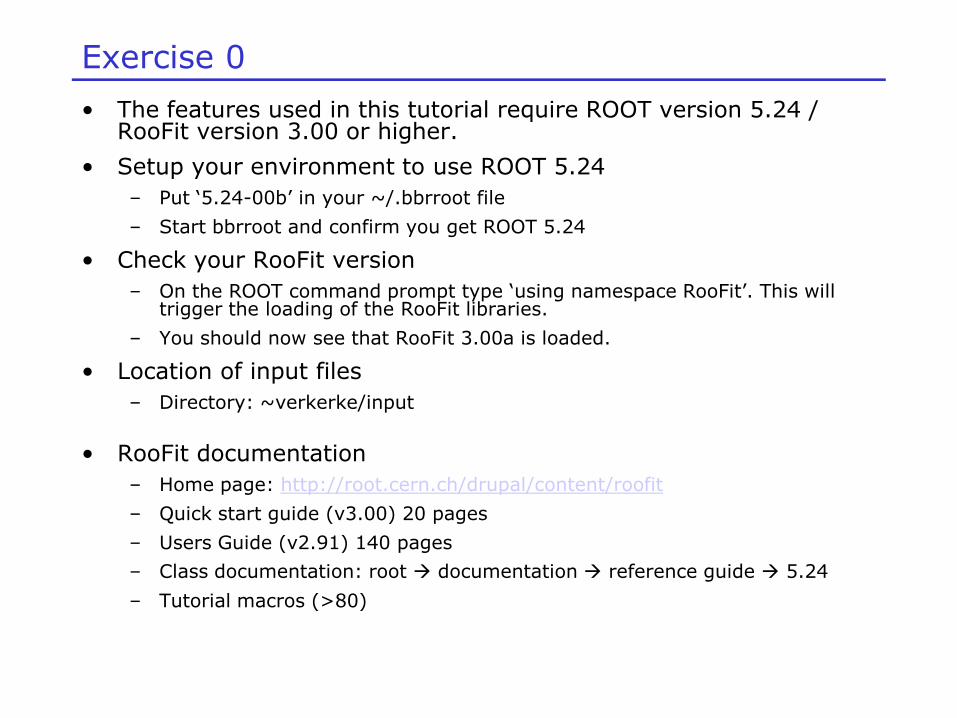
Exercise 0

• The features used in this tutorial require ROOT version 5.24 / RooFit version 3.00 or higher.

• Setup your environment to use ROOT 5.24– Put ‘5.24-00b’ in your ~/.bbrroot file

– Start bbrroot and confirm you get ROOT 5.24

• Check your RooFit version– On the ROOT command prompt type ‘using namespace RooFit’. This will

trigger the loading of the RooFit libraries.

– You should now see that RooFit 3.00a is loaded.

• Location of input files • Location of input files – Directory: ~verkerke/input

• RooFit documentation– Home page: http://root.cern.ch/drupal/content/roofit

– Quick start guide (v3.00) 20 pages

– Users Guide (v2.91) 140 pages

– Class documentation: root à documentation à reference guide à 5.24

– Tutorial macros (>80)

Exercise 1

• Take input file ex1.C, look at it and run it.

• Step 1 – Using the factory– Modify the code so that it uses the factory to create the pdf.

– Remove the code that creates the pdf directly and import() call.

– Run again to verify that you get the same result

• Step 2 – Adding background– Rename the Gaussian pdf from “model” to “signal”.

– Add an ArgusBG model named bkg to the workspace with m0=5.291 – Add an ArgusBG model named bkg to the workspace with m0=5.291 (fixed) and a slope of -40 with a range of [-100,0]

• look in $ROOTSYS/include for the constructor syntax and map that the corresponding factory call

– Create a sum of the signal and background with a signal fraction that is 20% (with range 0,1)

– Rerun the macro

– Add a plotOn() call that draws the background component of model using a Components() argument and give it a dashed linestyle (add LineStyle(kDashed)).

– Call Print() on the workspace to see the contents. Also call Print(“t”) to see the same contents shown as a tree structure

Exercise 1

• Step 3 – Making an extended ML fit– Rewrite the SUM() string so that it construct a pdf suitable for extended ML fitting: Multiply the signal pdf by Nsig (200 events, range 0,10000) and the background pdf by Nbkg (800 events, range 0,10000)

• Step 4 – Simple use of ranges– Define a ‘signal range’ in observable mes:

w.var(“mes”)->setRange(“signal”,5.27,5.29) ;

– Create an integral object that represents the fraction of background events in the signal range

w.factory(“int::sigRangeFrac(bkg,mes|signal,mes)”) ;

the first mes indicate which observable to integrate over, the second mes indicates which observables to normalize over. (Without a range specification this would result in 1 by construction)

– Retrieve the value of the fraction by calling w.function(“sigRangeFrac”)->getVal() ;

Exercise 1

– Now construct a formula named NsigRange that expresses the number of signal events in the signal range: use product operator prod::NsigRange(Nbkg,sigRangeFrac)

– Evaluate the NsigRange function in the workspace to count the number of signal events in the range [5.27,5.29]

• Step 5 – Linear error propagation (ROOT 5.25 only)– Now we calculate the error on NsigRange. To that end we first

need to save a RooFitResult object from the fitTo() operation: Save the RooFitResult* pointer returned by fitTo() in an object Save the RooFitResult* pointer returned by fitTo() in an object named fr, and add a Save() argument to fitTo() to instruct to make sure an fit resulted will be returned.

– Calculate the error on the number of signal events by callingw.function(“NsigRange”)->getPropagatedError(*fr) ;

Exercise 2

• Take input file ex2.C look at it and run it– The input macro constructs a B Decay distribution with mixing without

resolution effect (convolution with delta function). It then generates some data and plots the decay distribution of mixed and unmixed events separately, as well as the mixing asymmetry.

• Step 1 – Adding a resolution– Using the factory, construct a Gaussian resolution model (class

RooGaussModel) with mean 0 (fixed) and width 2 (floating, range 0.1-10) and change decay pdf to use that resolution model. Rerun the macro and observe the effect on the decay distributions and the asymmetry plot.asymmetry plot.

– Now construct a composite resolution model consisting of two Gaussians: 80% (fixed) of a narrow Gaussian (mean 0, width 1 (floating)) and the remainder a wide Gaussian (mean 0, width 5 (floating)). Rerun the macro and observe the effect on the decay distributions and the asymmetry plot.

• Step 2 – Visualize the correlation matrix– Look at the correlation matrix of the fit. To make a visual presentation

of the correlation matrix, save the RooFitResult object from the fitTo() command (don’t forget to add Save() as well) add the following code

gStyle->SetPalette(1) ;fr->correlationHist()->Draw(“colz”) ;

Exercise 2

– What are the largest correlations? • If correlations are very strong (>>0.9) the model may become unstable and it may

be worthwhile to fix one of the parameters in the fit.

This works best if the correlation is between two nuisance parameters (i.e. non-physics parameters such as the mistag rate)

If a correlation is between a parameter of interest (=physics, e.g. tau, ∆m) and a nuisance parameter (=others, e.g. mistag rate) fixing a nuisance parameter will strongly underestimate the uncertainty on physics parameter and you’ll need another strategy to control the error on the nuisance parameter.

• Step 3 – Visualize the uncertainty on the asymmetry• Step 3 – Visualize the uncertainty on the asymmetry– You can also visualize the uncertainty on the asymmetry curve

through linear propagation of the covariance matrix of the fit parameters. To do so duplicate the plotOn() call for the asymmetry curve in the macro and add the following argument to the first call

VisualizeError(*fr),FillColor(kOrange)) ;