introduction to the scattering matrix formalism · chapter 1 scattering matrix formalism 1.1...
TRANSCRIPT

Introduction to the Scattering MatrixFormalism
Fabrizio DolciniScuola Normale Superiore di Pisa, NEST (Italy)
Dipartimento di Fisica del Politecnico di Torino (Italy)
Lecture Notes for XXIII Physics GradDays, Heidelberg, 5-9 October 2009

Contents
1 Scattering Matrix Formalism 31.1 Introduction . . . . . . . . . . . . . . . . . . . . . . . . . . . . . . . . . . . . 31.2 Example: Ballistic Quantum Wire . . . . . . . . . . . . . . . . . . . . . . . . 4
1.2.1 The case with one impurity . . . . . . . . . . . . . . . . . . . . . . . 41.3 Relation between Transfer matrix and Scattering matrix . . . . . . . . . . . 7
1.3.1 General remarks . . . . . . . . . . . . . . . . . . . . . . . . . . . . . 71.3.2 Hybrid junction . . . . . . . . . . . . . . . . . . . . . . . . . . . . . . 9
1.4 Combining Scattering Matrices: The case with two impurities . . . . . . . . 121.4.1 Transmission Coefficient . . . . . . . . . . . . . . . . . . . . . . . . . 17
1.5 Properties of the Scattering Matrices: Unitarity and Onsager relations . . . . 191.6 Landauer-Buttiker formalism . . . . . . . . . . . . . . . . . . . . . . . . . . . 20
1.6.1 The single channel case . . . . . . . . . . . . . . . . . . . . . . . . . . 201.7 Current operator . . . . . . . . . . . . . . . . . . . . . . . . . . . . . . . . . 22
1.7.1 Definition . . . . . . . . . . . . . . . . . . . . . . . . . . . . . . . . . 221.7.2 Electrons with parabolic dispersion . . . . . . . . . . . . . . . . . . . 221.7.3 Expression in the Left Lead . . . . . . . . . . . . . . . . . . . . . . . 231.7.4 Expression in the Right Lead . . . . . . . . . . . . . . . . . . . . . . 26
1.8 Average Current and Non-linear Conductance . . . . . . . . . . . . . . . . . 271.8.1 Zero temperature limit . . . . . . . . . . . . . . . . . . . . . . . . . . 281.8.2 Source of Resistance . . . . . . . . . . . . . . . . . . . . . . . . . . . 281.8.3 Example. Fabry-Perot oscillations in carbon Nanotubes . . . . . . . . 30
1.9 Multi-channel case . . . . . . . . . . . . . . . . . . . . . . . . . . . . . . . . 321.9.1 Example: Quantum Point Contact in a Semiconductor 2DEG . . . . 36
2

Chapter 1
Scattering Matrix Formalism
1.1 Introduction
Let us consider a mesoscopic sample connected to two reservoirs on the Left(L) and Right(R),as shown in Fig.1.1.
mesoscopic sampleLEFT ELECTRODE
RIGHT ELECTRODELEAD LEAD
Figure 1.1: A mesoscopic sample connected to two (normal) metallic electrodes.
In experiments the typical size reservoirs is wide compared to the typical cross-section ofthe mesoscopic conductor. Consequently, the mesoscopic system represents only a smallperturbation for the reservoirs, which can thus be described in terms of an equilibrium state,characterized by chemical potentials µL and µR and temperatures TL and TR, respectively.The distribution functions of electrons in the reservoirs are therefore Fermi distributionfunctions
fX(E) =1
1 + e(E−µX)/kBTXX = L/R (1.1)
It is worth emphasizing the differences between the reservoirs and the mesoscopic sample:
• While in the mesoscopic sample no inelastic processes occur, in the reservoirs inelasticprocesses do occur, for otherwise no equilibrium state could be established.
• Furthermore, electrodes are characterized by a large number of modes, which are en-ergetically very closely spaced, whereas the mesoscopic system has a finite number ofmodes.
3

4 Example: Ballistic Quantum Wire
The contacts between the mesoscopic conductor and the reservoirs can be schematized asideal narrow channels widening into the large reservoirs, which are called leads, or contactregions .
We suppose for simplicity that the temperatures in the two electrodes are the same TL =TR = T , whereas we apply a voltage bias V between the two electrodes
V = (µL − µR)/q (1.2)
where q is the elementary electron charge (q = e = |e| or q = −e = −|e| depending on theconvention used in the literature). The voltage induces a current I through the sample anddrives it into a non-equilibrium state. The purpose is to determine the transport properties(average current, current fluctuations, etc.) as a function of the applied bias V and of thetypical parameters characterizing the mesoscopic system.
1.2 Example: Ballistic Quantum Wire
1.2.1 The case with one impurity
Let us consider free electrons with parabolic dispersion and with one δ-like impurity locatedat x = x0; in second quantization the Hamiltonian reads
H =
∫ +∞
−∞Ψ†(x)
(− ~2
2m
∂2
∂x2+ Λδ(x− x0)
)Ψ(x) dx
where the electron field fulfills anti-commutation relationsΨ(x),Ψ†(y)
= δ(x− y) (1.3)
Introducing
Λ = Λ2m
~2(1.4)
we can also rewrite
H = − ~2
2m
∫ +∞
−∞Ψ†(x)
(∂2Ψ(x)
∂x2+ Λ δ(x− x0)Ψ(x)
)dx
The equation of motion for the field Ψ reads
i~Ψ = [Ψ,H] (1.5)
i.e.
i~Ψ(x, t) = − ~2
2m
(∂2
∂x2Ψ(x, t) + Λδ(x− x0)Ψ(x, t)
)(1.6)
Fabrizio Dolcini, Superconductivity in Mesoscopic Systems, Lecture Notes for XXIII Physics GradDays, Heidelberg

Chap. 1. Scattering Matrix Formalism 5
From this equation we observe that ∂2xΨ has a δ-like singularity, implying that ∂xΨ is discon-
tinuous at x = x0. The field Ψ itself, in contrast, is continuous. Integrating around x = x0
we obtain that
∂xΨ(x+0 ) − ∂xΨ(x−0 ) = ΛΨ(x0) (1.7)
Thus, the equation of motion (1.6) is equivalent toi~Ψ(x, t) = − ~2
2m∂2
∂x2 Ψ(x, t) x 6= x0
Ψ(x+0 , t) = Ψ(x−0 , t)
∂xΨ(x+0 , t) − ∂xΨ(x−0 , t) = ΛΨ(x0, t)
In order to solve these equations, we make the following Ansatz
Ψk(x, t) = e−iEkt/~
aLk e
ikx + bLk e−ikx x < x0
bRk eikx + aRk e
−ikx x > x0
(1.8)
where
Ek =~2k2
2m(1.9)
which satisfies the first condition.The second and third conditions respectively yield
aLk eikx0 + bLk e
−ikx0 = bRk eikx0 + aRke
−ikx0
ik(bRk e
ikx0 − aRk e−ikx0
)− ik
(aLk e
ikx0 − bLke−ikx0
)= Λ
(aLk e
ikx0 + bLk e−ikx0
)(1.10)
The solution of this set of linear equations for the amplitude operators can easily be found(see below) and reads bRk
aRk
= Mk
aLk
bLk
(1.11)
where the matrix Mk
Mk =
1 + Λ2ik
Λ2ike−2ikx0
− Λ2ike2ikx0 1− Λ
2ik
(1.12)
Fabrizio Dolcini, Superconductivity in Mesoscopic Systems, Lecture Notes for XXIII Physics GradDays, Heidelberg

6 Example: Ballistic Quantum Wire
is called the Transfer Matrix, for it describes how the amplitude operators on the left ofthe impurity are ’transfered’ to the ones on the right of the impurity.We notice that
• the Transfer Matrix exhibits the following properties of the transfer matrix:
detMk = 1 M21 = M∗12 (1.13)
• the order of a, b operators appearing in Eq.(1.11) is different on the left and right side.This is because typically Transfer Matrix is defined as relating corresponding velocityamplitudes. A right-moving electron is described by bRk on the right of the impurity,and by aRk on the left of the impurity.
Proof of Eq.(1.10)Starting from Eqs.(1.10) one can now introduce
a′Lk = aLk eikx0
b′Lk = bLk e−ikx0
b′Rk = bRk eikx0
a′Rk = aRk e−ikx0
(1.14)
and reexpress the above equations in these new variablesa′Lk + b′Lk = b′Rk + a′Rk
ik(b′Rk − a′Rk
)− ik
(a′Lk − b′Lk
)= Λ
(a′Lk + b′Lk
)i.e.
a′Lk + b′Lk = b′Rk + a′Rk
a′Lk
(1 +
Λik
)− b′Lk
(1− Λ
ik
)= b′Rk − a′Rk
We have now two equations for four unknowns. In order to determine the transfer matrix we haveto express the variables of the RIGHT-part as a function the the ones in the LEFT part. It istherefore straightforward to replace the above equations with their sum and difference
b′Rk =(
1 + Λ2ik
)a′Lk + Λ
2ik b′Lk
a′Rk = − Λ2ik a
′Lk +
(1− Λ
2ik
)b′Lk
Fabrizio Dolcini, Superconductivity in Mesoscopic Systems, Lecture Notes for XXIII Physics GradDays, Heidelberg

Chap. 1. Scattering Matrix Formalism 7
Coming now back to the original variables (1.14) the latter equations can be rewritten asbRk =
(1 + Λ
2ik
)aLk + Λ
2ik e−2ikx0 bLk
aRk = − Λ2ik e
2ikx0 aLk +(
1− Λ2ik
)bLk
which are simply Eqs.(1.10) written in matrix form.
1.3 Relation between Transfer matrix and Scattering
matrix
1.3.1 General remarks
The Transfer matrix expresses the coefficients of the states on the right side of scatterer interms of the coefficients of the same states on the left side of the scatterer:
bR
aR
=
M11 M12
M21 M22
· aL
bL
(1.15)
The relations (1.15) between operators are linear. It is thus easy to express the same relationsalso in different equivalent ways. In particular, one can expresses the outgoing state operatorsas a function of the incoming state operators, bL
bR
=
S11 S12
S21 S22
· aL
aR
(1.16)
and the matrix S is called the Scattering Matrix.It is straightforward to verify that the S-matrix can be expressed in terms of the Transfermatrix entries as follows:
S =1
M22
−M21 1
1 M12
(1.17)
where we have used the property:detM = 1 (1.18)
Usually the Scattering matrix entries are denoted as
S =
(r t′
t r′
)(1.19)
Fabrizio Dolcini, Superconductivity in Mesoscopic Systems, Lecture Notes for XXIII Physics GradDays, Heidelberg

8 Relation between Transfer matrix and Scattering matrix
where tk, t′k and rk, r
′k are transmission and reflection amplitudes. Let us for instance assume
to ’prepare’ the incoming wave packet as coming from LEFT (we thus set aR = 0). Thenthe transmission and reflection coefficients read
T = |t|2 =
∣∣∣∣ 1
M22
∣∣∣∣2
R = |r|2 =
∣∣∣∣−M21
M22
∣∣∣∣2 =
∣∣∣∣M12
M22
∣∣∣∣2(1.20)
Exploiting the property:
M∗21 = M12 (1.21)
one can observe that the same result is obtained if the incoming wave packet comes fromRIGHT.
Example: Scattering Matrix and Transmission Coefficient for the case with oneimpurity
• In the case described above of a quantum wire with one single impurity the Scatteringmatrix can be obtained using the Transfer Matrix and applying the relation (1.17)between Scattering and Transfer matrices
S =
Λ2ik−Λ
e2ikx0 2ik2ik−Λ
2ik2ik−Λ
Λ2ik−Λ
e−2ikx0
(1.22)
• Importantly we observe that the Scattering matrix is unitary
S†S = I
• The transmission coefficient is easily computed inserting Eqs.(1.12) into Eq.(1.20).
T =1
1 + Λ2
4k2
=8mE
~2
8mE~2 + Λ2
=2~2
mE
2~2
mE + Λ2
(1.23)
We observe that the transmission coefficient does not depend on the position x0 of theimpurity.
Fabrizio Dolcini, Superconductivity in Mesoscopic Systems, Lecture Notes for XXIII Physics GradDays, Heidelberg

Chap. 1. Scattering Matrix Formalism 9
0 2 4 6 8 100.0
0.2
0.4
0.6
0.8
1.0
λ=.01
λ=3.0
λ=1T
EFigure 1.2: The Transmission coefficient for a quantum wire with parabolic dispersion inthe presence of one impurity.
1.3.2 Hybrid junction
• Let us consider a hybrid junction between two different materials (e.g. two differentsemiconductors), characterized by different effective masses, i.e. by different parabolicdispersion. Let us assume that the junction is ideal and that no backscattering term(like the δ-like impurity in the previous example) is present. In general this will notbe the case, but this is unimportant for what we want to point out here. At a givenvalue of the energy E the characteristic momenta (and velocities) in the two regionsforming the junction are different, due to the different dispersion relations. Since thesystem breaks translational invariance, momentum is not conserved and is not a goodquantum number, whereas energy is (see Fig.1.3).
• Model: The hybrid junction can be modeled as a system with a space-dependent mass
H =
∫ +∞
−∞Ψ†(x)
∂
∂x
(− ~2
2m(x)
∂Ψ(x)
∂x
)dx (1.24)
where the effective mass reads
m(x) = mL θ(x− x0) +mR θ(x0 − x) (1.25)
The equation of motion for the field Ψ reads
Fabrizio Dolcini, Superconductivity in Mesoscopic Systems, Lecture Notes for XXIII Physics GradDays, Heidelberg

10 Relation between Transfer matrix and Scattering matrix
vRvL
kL kR
mRmL
Figure 1.3: A junction between different materials.
i~Ψ(x, t) =∂
∂x
(− ~2
2m(x)
∂Ψ(x, t)
∂x
)x 6= x0
Ψ(x+0 , t) = Ψ(x−0 , t)
1
mR
∂xΨ(x+0 , t) =
1
mL
∂xΨ(x−0 , t)
To solve the above relation we make the following Ansatz
Ψ(x, t) = e−iEt/~
aLkL e
ikLx + bLkL e−ikLx x < x0
bRkR eikRx + aRkR e
−ikRx x > x0
(1.26)
where
kL =1
~√
2mLE kR =1
~√
2mRE (1.27)
It is straightforward to see that the solution is bLkL
bRkL
= SkLkR ·
aLkL
aRkL
(1.28)
with
SkLkR =1
vL + vR
(vL − vR) e2ikLx0 2vR ei(kL−kR)x0
2vL ei(kL−kR)x0 −(vL − vR) e−2ikRx0
(1.29)
where
vL(E) =~kLmL
vR(E) =~kRmR
(1.30)
Fabrizio Dolcini, Superconductivity in Mesoscopic Systems, Lecture Notes for XXIII Physics GradDays, Heidelberg

Chap. 1. Scattering Matrix Formalism 11
Here the two subscripts (kLkR) in SkLkR remind that, differently from the previous caseof a single impurity, momentum is not conserved in this problem. Importantly, onecan easily prove that this scattering matrix SkLkR is not unitary.
• Motivated by the remark that energy (and not momentum) is conserved, we try tointroduce operators that are related to energy. Let us then pass from momentum labelto energy label. In doing that, we also pass to the continuum∑
k
... =Ω
2π
∫dk... =
Ω
2π
∫1
~v(E)dE... (1.31)
We notice that
aLk, a†Lk′ = bLk, b
†Lk′ = δk,k′ =
2π
Ωδ(k − k′) =
2π
Ω~v(E)δ(E − E ′) , (1.32)
with
v(E) =1
~
∣∣∣∣∂E∂k∣∣∣∣ , (1.33)
We can thus introduce energy amplitude operators aXE and bXE, defined through therelations1
aLkL =√
2π~vLΩ
aLE
bLkL =√
2π~vLΩ
bLE
bRkR =√
2π~vRΩ
bRE
bRkR =√
2π~vRΩ
bRE
(1.34)
They obey the following anticommutation relatiosn
aLE, a†LE′ = bLE, b
†LE′ = δ(E − E ′) aLE, bLE′ = aLE, b
†LE′ = 0(1.35)
In terms of the new operators Eqs.(1.28) and (1.29) are easily rewritten as bLE
bRE
= S(E) ·
aLE
aRE
(1.36)
with a new scattering matrix
S(E) =1
vL + vR
(vL − vR) e2ikLx0 2√vRvL e
i(kL−kR)x0
2√vRvL e
i(kL−kR)x0 −(vL − vR) e−2ikRx0
(1.37)
1Notice that in Eq.(1.72) the velocity is independent of the LEFT/RIGHT or IN/OUT; it only dependson the energy. This is equivalent to assuming that the band is symmetric for k → −k. This is also consistentwith Eq.(1.65), where only one energy appears.
Fabrizio Dolcini, Superconductivity in Mesoscopic Systems, Lecture Notes for XXIII Physics GradDays, Heidelberg

12 Combining Scattering Matrices: The case with two impurities
where kL and kR are related to energy through Eq.(1.27). Notice that, due to the factthat velocities are different, the matrix (1.37) is not simply the same matrix (1.29)re-expressed in terms of energy E. Importantly the scattering matrix (1.37) for thenew energy operators is unitary.
• One can wonder: why the previous matrix (1.29) was not unitary? Why a simpleredefinition (1.34) of the operators led unitarity emerge?
v1dt v2dt
Figure 1.4: Flux conservation.
This can be understood as follows: In hybrid systems, such as heterojunctions betweentwo different semiconductors or junctions between normal and a superconductors, den-sity is typically not conserved across the junction. Indeed, as shown in Fig.1.3, ata given energy we have different kF ’s in the two sides of the junction, i.e. differentelectron densities. This is quite similar to what happens to an incompressible fluidflowing through a pipeline with inhomogeneous velocities: in order for the total num-ber of particles to be preserved, the density is not uniform. In contrast the flux ρv ispreserved: the lower the velocity the higher the density (see Fig.1.4). In our case theflux is simply the current density, which is conserved across the junction.
J = qvΨ†Ψ ∼ q v a†k ak = qva†E√2π~v
aE√2π~v
=q
ha†E aE
The conservation of J implies the unitarity for the scattering matrix connecting a†Eand b†E operators: the incoming flux must equal the outgoing flux. For this reason thescattering matrix is usually meant as refereed to the energy amplitude operators, andnot to the a†k operators.
1.4 Combining Scattering Matrices: The case with two
impurities
Let us consider free electrons with parabolic dispersion, but with two δ-like impurities locatedat x = x1 and x = x2 (with x1 < x2).This could be for instance a nice toy model to account for the presence of non-ideal contactsbetween a ballistic quantum wire and the leads (notice that ’non-ideal’ means T < 1; weshall see, however, that even for ideal contacts with T = 1 there exists an intrinsic quantum
Fabrizio Dolcini, Superconductivity in Mesoscopic Systems, Lecture Notes for XXIII Physics GradDays, Heidelberg

Chap. 1. Scattering Matrix Formalism 13
of resistance RQ).The length of the quantum wire is then
L = x2 − x1 (length of the wire) (1.38)
The Hamiltonian then reads:
H = − ~2
2m
∫ +∞
−∞Ψ†(x)
∂2
∂x2Ψ(x) dx + Λ
(Ψ†(x1)Ψ(x1) + Ψ†(x2)Ψ(x2)
)Introducing again Eq.(1.4), i.e.
Λ = Λ2m
~2(1.39)
and integrating the equation of motion around x = x1 and then around x = x2, we obtainthe following conditions
i~Ψ(x, t) = − ~2
2m
∂2
∂x2Ψ(x, t) x 6= x1, x2
Ψ(x) continuous at x = x1 and at x = x2
∂xΨ(x+1 ) − ∂xΨ(x−1 ) = ΛΨ(x1)
∂xΨ(x+2 ) − ∂xΨ(x−2 ) = ΛΨ(x2)
The following Ansatz
Ψk(x, t) = e−iEkt/~
aLk e
ikx + bLk e−ikx x < x1
γ+k e
ikx + γ−k e−ikx x1 < x < x2
bRk eikx + aRk e
−ikx x > x2
(1.40)
fulfills the first condition with energy:
Ek =~2k2
2m(1.41)
The second, third and forth conditions respectively yield
aLk eikx1 + bLk e
−ikx1 = γ+k e
ikx1 + γ−k e−ikx1
γ+k e
ikx2 + γ−k e−ikx2 = bRk e
ikx2 + aRke−ikx2
ik(γ+k e
ikx1 − γ−k e−ikx1
)− ik
(aLk e
ikx1 − bLke−ikx1
)= Λ
(aLk e
ikx1 + bLk e−ikx1
)ik(bRk e
ikx2 − aRk e−ikx2
)− ik
(γ+k e
ikx2 − γ−k e−ikx2
)= Λ
(bRk e
ikx2 + aRk e−ikx2
)(1.42)
Fabrizio Dolcini, Superconductivity in Mesoscopic Systems, Lecture Notes for XXIII Physics GradDays, Heidelberg

14 Combining Scattering Matrices: The case with two impurities
This linear system of equations can be solved straightforwardly (see below for explicit deriva-tion), and one finds that
γ+k
γ−k
=
(
1 + Λ2ik
)Λ
2ike−2ikx1
− Λ
2ike2ikx1
(1− Λ
2ik
)
︸ ︷︷ ︸Mk(x1) = Transfer Matrix at x1
·
aLk
bLk
(1.43)
bRk
aRk
=
(
1 + Λ2ik
)Λ
2ike−2ikx2
− Λ2ike2ikx2
(1− Λ
2ik
)
︸ ︷︷ ︸Mk(x2) = Transfer Matrix at x2
·
γ+k
γ−k
(1.44)
where the transfer matrices Mk(x1) and Mk(x2) are the single impurity transfer matrices(see Eq.(1.12)) respectively at x1 and x2. The whole Transfer Matrix bRk
aRk
= Mk ·
aLk
bLk
(1.45)
is thus obtained as the product
Mk = Mk(x2) ·Mk(x1) = (1.46)
=
(
1 + Λ2ik
)2
−(
Λ2ik
)2
e−2ik(x2−x1) Λ2ik
((1 + Λ
2ik
)e−2ikx1 +
(1− Λ
2ik
)e−2ikx2
)
− Λ2ik
((1− Λ
2ik
)e2ikx1 +
(1 + Λ
2ik
)e2ikx2
) (1− Λ
2ik
)2
−(
Λ2ik
)2
e2ik(x2−x1)
We now pass to energy amplitude operators
aLk =√
2π~vΩ
aLE
bLk =√
2π~vΩ
bLE
bRk =√
2π~vΩ
bRE
bRk =√
2π~vΩ
bRE
(1.47)
Fabrizio Dolcini, Superconductivity in Mesoscopic Systems, Lecture Notes for XXIII Physics GradDays, Heidelberg

Chap. 1. Scattering Matrix Formalism 15
Since in this case the velocity
vE =~kEm
=
√2E
m(1.48)
is the same everywhere, the Trasfer Matrix for the aXE and bXE operators is simply Eq.(1.46),expressed in terms of energy E. Recalling that
Λ = Λ2m
~2(1.49)
one rewrites Eq. (1.46) as
ME =
=
(
1 + Λi~vE
)2
−(
Λi~vE
)2
e−2ik(x2−x1) Λi~vE
((1 + Λ
i~vE
)e−2ikx1 +
(1− Λ
i~vE
)e−2ikx2
)
− Λi~vE
((1− Λ
i~vE
)e2ikEx1 +
(1 + Λ
i~vE
)e2ikx2
) (1− Λ
i~vE
)2
−(
Λi~vE
)2
e2ikE(x2−x1)
It is straightforward to verify that M∗E = ME; moreover, since the determinant of each
ME(xi)’s equals 1, one also has that detME = 1.
Proof of Eqs.(1.44) and (1.44):Consider Eq.(1.42) and introduce
a′Lk = aLk eikx1
b′Lk = bLk e−ikx1
b′Rk = bRk eikx2
a′Rk = aRk e−ikx2
(1.50)
and rewrite the equations as
a′Lk + b′Lk = γ+k e
ikx1 + γ−k e−ikx1
γ+k e
ikx2 + γ−k e−ikx2 = b′Rk + a′Rk
ik(γ+k e
ikx1 − γ−k e−ikx1
)− ik
(a′Lk − b′Lk
)= Λ
(a′Lk + b′Lk
)ik(b′Rk − a′Rk
)− ik
(γ+k e
ikx2 − γ−k e−ikx2
)= Λ
(b′Rk + a′Rk
)Fabrizio Dolcini, Superconductivity in Mesoscopic Systems, Lecture Notes for XXIII Physics GradDays, Heidelberg

16 Combining Scattering Matrices: The case with two impurities
i.e.
a′Lk + b′Lk = γ+k e
ikx1 + γ−k e−ikx1
b′Rk + a′Rk = γ+k e
ikx2 + γ−k e−ikx2
(1 +
Λik
)a′Lk −
(1− Λ
ik
)b′Lk = γ+
k eikx1 − γ−k e
−ikx1
(1− Λ
ik
)b′Rk −
(1 +
Λik
)a′Rk = γ+
k eikx2 − γ−k e
−ikx2
These are 4 equations for 6 unknowns; in order to determine the transfer matrix, we express noweverything in terms of the variables in the LEFT side; thus, we proceed as follows:
I → e−ikx1( I + III )
III → eikx1( I − III )
II →
(1− Λ
ik
)II − IV
IV →
(1 +
Λik
)II + IV
obtaining
γ+k = e−ikx1
((1 +
Λ2ik
)a′Lk +
Λ2ik
b′Lk
)
γ−k = eikx1
(− Λ
2ika′Lk +
(1− Λ
2ik
)b′Lk
)
a′Rk = − Λ2ik
eikx2 γ+k +
(1− Λ
2ik
)e−ikx2 γ−k
b′Rk =
(1 +
Λ2ik
)eikx2 γ+
k +Λ
2ike−ikx2 γ−k
(1.51)
Fabrizio Dolcini, Superconductivity in Mesoscopic Systems, Lecture Notes for XXIII Physics GradDays, Heidelberg

Chap. 1. Scattering Matrix Formalism 17
or, in matrix form: γ+k
γ−k
=
e−ikx1
(1 + Λ
2ik
)e−ikx1 Λ
2ik
−eikx1Λ
2ikeikx1
(1− Λ
2ik
) ·
a′Lk
b′Lk
b′Rk
a′Rk
=
eikx2
(1 + Λ
2ik
)e−ikx2 Λ
2ik
− Λ2ike
ikx2 e−ikx2
(1− Λ
2ik
) ·
γ+k
γ−k
By recalling the definition (1.50), one can see that the above equations yield (1.43) and (1.44).
1.4.1 Transmission Coefficient
The transmission coefficient is easily computed inserting the entry M22 of Eq.(1.50) intoEq.(1.20)
T =
∣∣∣∣ 1
M22
∣∣∣∣2 =1∣∣∣∣(1− Λ
i~v(E)
)2
−(
Λi~v(E)
)2
e2ikEL
∣∣∣∣2One has:∣∣∣∣∣(
1− Λ
i~v(E)
)2
−(
Λ
i~v(E)
)2
e2ikEL
∣∣∣∣∣2
=
=
(1 +
(Λ
~vE
)2)2
+
(Λ
~vE
)4
+
(Λ
~vE
)2[(
1− Λ
i~vE
)2
e−2ikEL +
(1 +
Λ
i~vE
)2
e+2ikEL
]=
= 1 + 2
(Λ
~vE
)2
+ 2
(Λ
~vE
)4
+
(Λ
~vE
)2[
2
(1−
(Λ
~vE
)2)
cos 2kEL+ 4Λ
~vEsin 2kEL
]=
= 1 + 2
(Λ
~vE
)2
+ 2
(Λ
~vE
)4
+
(Λ
~vE
)2[
2
(1−
(Λ
~vE
)2)(
2 cos2 kEL− 1)
+8Λ
~vEsin kEL cos kEL
]=
= 1 + 4
(Λ
~vE
)4
+ 4
(Λ
~vE
)2(
1−(
Λ
~vE
)2)
cos2 kEL + 8
(Λ
~vE
)3
sin kEL cos kEL =
= 1 + 4
(Λ
~vE
)4
sin2 kEL + 4
(Λ
~vE
)2
cos2 kEL + 8
(Λ
~vE
)3
sin kEL cos kEL =
= 1 + 4
(Λ
~vE
)2[(
Λ
~vE
)2
sin2 kEL + cos2 kEL + 2Λ
~vEsin kEL cos kEL
]=
= 1 + 4
(Λ
~vE
)2 [cos kEL +
Λ
~vEsin kEL
]2
whence
T (E) =1
1 + 4(
Λ~vE
)2 [cos kEL + Λ
~vE sin kEL]2 (1.52)
Fabrizio Dolcini, Superconductivity in Mesoscopic Systems, Lecture Notes for XXIII Physics GradDays, Heidelberg

18 Combining Scattering Matrices: The case with two impurities
We now recall that the typical energy range we are interested in (temperature and appliedvoltage) are much smaller than the equilibrium Fermi energy. We can thus write
E = εF + ξ |ξ| εF (1.53)
and therefore we have
kE =
√2mE
~=
√2m(εF + ξ)
~=
=1
~
√2mεF
(1 +
ξ
εF
)=
[use kF =1
~√
2mεF ]
= kF
√1 +
ξ
εF=
' kF
(1 +
ξ
2εF
)=
[use vF =~kFm
and 2εF = ~vFkF ]
= kF
(1 +
ξ
~vFkF
)=
= kF +ξ
~vF(1.54)
and one can well approximate Eq.(1.52) as
T (εF + ξ) ' 1
1 + 4λ2[cos[kFL+ ξ
EL] + λ sin[kFL+ ξ
EL]]2 (1.55)
where we have defined
EL = ~ωL =~vFL
(1.56)
and
λ =Λ
~vF(1.57)
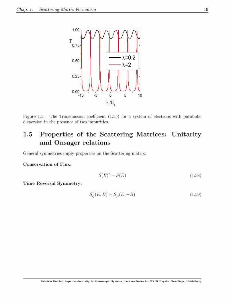
Here EL is the energy associated with the length of the wire (distance between the twocontact impurities), which is the natural characteristic lengthscale in this problem. We thusobserve that the transmission coefficient is an oscillatory function with a typical period givenby EL, as shown in Fig.1.5.
Fabrizio Dolcini, Superconductivity in Mesoscopic Systems, Lecture Notes for XXIII Physics GradDays, Heidelberg
Chap. 1. Scattering Matrix Formalism 19
-10 -5 0 5 100.00
0.25
0.50
0.75
1.00
T
E /EL
λ=0.2 λ=2
Figure 1.5: The Transmission coefficient (1.55) for a system of electrons with parabolicdispersion in the presence of two impurities.
1.5 Properties of the Scattering Matrices: Unitarity
and Onsager relations
General symmetries imply properties on the Scattering matrix:
Conservation of Flux:
S(E)† = S(E) (1.58)
Time Reversal Symmetry:
S†ij(E;B) = Sji(E;−B) (1.59)
Fabrizio Dolcini, Superconductivity in Mesoscopic Systems, Lecture Notes for XXIII Physics GradDays, Heidelberg
20 Landauer-Buttiker formalism
1.6 Landauer-Buttiker formalism
1.6.1 The single channel case
We consider independent electrons in one dimension, in the presence of scatterers. Forsimplicity we assume that we have only one band, in which we have IN-coming and OUT-going particles. Examples of this situation are given in sec.1.2 for electrons in the continuumwith parabolic dispersion. We wish here to define the general framework to treat thesemodels. Following Blanter and Buttiker, we denote:
a ↔ INoperators
b ↔ OUT
(1.60)
Similarly we shall denote the eigenfunctions asα(x) ↔ IN
eigenfunctionsβ(x) ↔ OUT
(1.61)
Once the location with respect to the set of scatterers is fixed (i.e. whether LEFT or RIGHT),the IN and OUT states are determined: for instance, for electrons with parabolic dispersion,one has
for k ≥ 0
αRkR(x) =
1√Ωe−ikRx αLkL(x) =
1√ΩeikLx
βRkR(x) =1√ΩeikRx βLkL(x) =
1√Ωe−ikLx
(1.62)
As the examples discussed in the previous sections suggest, the field operator in the LEFTand in the RIGHT lead can be respectively written as:
Ψ(x ∈ L, t) =∑k≥0
(αLkL(x) aLkL(t) + βLkL(x) bLkL(t)
)= (1.63)
=∑k≥0
e−iEkt/~(αLkL(x) aLkL + βLkL(x) bLkL
)= (1.64)
=1√Ω
∑k≥0
e−iEkt/~(eikLx aLkL + e−ikLx bLkL
)(1.65)
Ψ(x ∈ R, t) =∑k≥0
(αRk(x) aRkR(t) + βRk(x) bRkR(t)
)= (1.66)
=∑k≥0
e−iEkt/~(αRk(x) aRkR + βRkR(x) bRkR
)(1.67)
=1√Ω
∑k≥0
e−iEkt/~(e−ikRx aRkR + eikRx bRkR
)(1.68)
Fabrizio Dolcini, Superconductivity in Mesoscopic Systems, Lecture Notes for XXIII Physics GradDays, Heidelberg

Chap. 1. Scattering Matrix Formalism 21
where the operators aXk’s and bXk’s (X = L/R) fulfill
aXkX , a†Y k′
Y = δXY δk,k′ (1.69)
bXkX , b†Y k′ = δX,Y δk,k′ (1.70)
aXkX , bXk′X = aXkX , b
†Xk′
X = 0 (1.71)
Since we have explicitly separated IN and OUT states, the sum over the momentumonly runs on positive k’s.
Explicit realizations of Eqs.(1.63)-(1.68) have been provided in the previous sections; inparticular i) in (1.8) and (1.40) for electrons with parabolic dispersion in the presence of oneand two impurities.
We have also seen that it is customary to introduce energy amplitude operatorsaXE = 1√
2πΩ
~vX(E)aXkX
X = L/R
bXE = 1√2πΩ
~vX(E)bXkX
(1.72)
which obey anticommutations relations
aX kX, a†Xk′
X = bX kX
, b†Xk′X = δkX ,k′
X=
2π
Ωδ(kX − k′X) =
2π
Ω~v(E)δ(E − E ′) , (1.73)
Similarly we also relabel αLkL(x) = αLEL(x)
βLkL(x) = βLEL(x)(1.74)
where kE ≥ 0 denotes the positive momentum corresponding to the energy E (mostra infigura).We thus obtain that Eqs.(1.65) and (1.68) can be rewritten as
Ψ(x ∈ L, t) =1√2π~
∫ ET
EB
dE√vL(E)
e−iEt/~(eikLEx aLE + e−ikLEx bLE
)(1.75)
Ψ(x ∈ R, t) =1√2π~
∫ ET
EB
dE√vR(E)
e−iEt/~(e−ikREx aRE + eikREx bRE
)(1.76)
where EB and ET are respectively the bottom and top values of the energy band.
Fabrizio Dolcini, Superconductivity in Mesoscopic Systems, Lecture Notes for XXIII Physics GradDays, Heidelberg

22 Current operator
1.7 Current operator
1.7.1 Definition
The current operator is defined as
I(x, t) = qN∑i=1
1
2(δ(x− xi)vi + viδ(x− xi)) (1.77)
where vi is the velocity operator of the i-th particle, and the symmetrized form is required,because in general vi and δ(x−xi) do not commute. It is important to realize that the formof the velocity operator is not unique, it depends on the context. As a rule, in k-space thevelocity is given by:
vk =1
~∂Ek∂k
(1.78)
1.7.2 Electrons with parabolic dispersion
In the case of fermions with parabolic dispersion one has Ek = ~2k2/2m one gets vk = ~k/m,which yields, in x-space
v =p
m(1.79)
so, in second quantized formalism, one has:
I(x, t) = −i~ q
2m
(Ψ†(x, t)
∂Ψ
∂x(x, t)− ∂Ψ†
∂x(x, t)Ψ(x, t)
)(1.80)
The current is typically measured in the leads. Replacing Eq.(1.75) and Eq.(1.76) intothe general expression (1.80) we have that the current in the LEFT and RIGHT leadsrespectively.
Fabrizio Dolcini, Superconductivity in Mesoscopic Systems, Lecture Notes for XXIII Physics GradDays, Heidelberg

Chap. 1. Scattering Matrix Formalism 23
1.7.3 Expression in the Left Lead
Replacing Eq.(1.75) into Eq.(1.80) we obtain the current in the left lead
I(x ∈ L, t) .=
1
2π~· −i~q
2m
∫ ∫dE dE ′√v(E)v(E ′)
ei(E−E′)t/~ ·
·i(kE′ + kE) e−i(kE−kE′ )x a†LE aLE′ − i(kE′ + kE) ei(kE−kE′ )x b†LE bLE′+
−i(kE′ − kE) e−i(kE+kE′ ) a†LE bLE′ + i(kE′ − kE) ei(kE+kE′ )x b†LE aLE′
=
.=
q
2π~
∫ ∫dE dE ′√v(E)v(E ′)
ei(E−E′)t/~ ·
·
~(kE + kE′)
2m
[e−i(kE−kE′ )x a†LE aLE′ − ei(kE−kE′ )x b†LE bLE′+
]+
~(kE − kE′)
2m
[− e−i(kE+kE′ )x a†LE bLE′ + ei(kE+kE′ )x b†LE aLE′
](1.81)
Recalling now that
v(E) =~kEm
one obtains
I(x ∈ L, t) .=
q
2π~
∫ ∫dE dE ′ ei(E−E
′)t/~ · (1.82)
·
v(E) + v(E ′)
2√v(E)v(E ′)
[e−i(kE−kE′ )x a†LE aLE′ − ei(kE−kE′ )x b†LE bLE′+
]+v(E)− v(E ′)
2√v(E)v(E ′)
[− e−i(kE+kE′ )x a†LE bLE′ + ei(kE+kE′ )x b†LE aLE′
]
Linearization
We now observe that typically the energies which are relevant to most of the physical quan-tities are those in a narrow range with respect to the Fermi energy. We can thus linearizearound the Fermi energy and approximate
vL(E) ' vLF (1.83)
and
kLE − kLE′ ' E − E ′
~vLF(1.84)
so that Eq.(1.82) simplifies to
I(x ∈ L, t) .=
q
2π~
∫ ∫dE dE ′ ei(E−E
′)t/~ ·e−i(E−E
′)x/~vF a†LE aLE′ − ei(E−E′)x/~vF b†LE bLE′
(1.85)
Notice that the linearized form (1.85) looks much simpler than the general expression (1.82),although linearization is not a necessary condition to apply Landauer-Buttiker formalism.
Fabrizio Dolcini, Superconductivity in Mesoscopic Systems, Lecture Notes for XXIII Physics GradDays, Heidelberg

24 Current operator
The linearization procedure is equivalent to treating Dirac electrons, which are characterizedby a linear dispersion relation Ek = ~vFk, for which the velocity is operator
vk = vF (1.86)
i.e. a constant. The situation is in fact slightly more complicated, because one has twobranches, i.e. right and left movers Ψ→ and Ψ←, with velocities vk = ±vF respectively.Thus, the form of the current operator in the second quantized form for Dirac fermionsreads
I(x, t) = qvF(Ψ†→(x, t)Ψ→(x, t) − Ψ†←(x, t)Ψ←(x, t)
)(1.87)
The definition (1.87) of the current, together with the expression for the density:
ρ(x, t) = q(Ψ†→(x, t)Ψ→(x, t) + Ψ†←(x, t)Ψ←(x, t)
)ensures the continuity equation
∂tρ = −∂xJ
for the solutions of the Dirac equation.
Use of the Scattering Matrix
Suppose that we now want to compute the average current in the (say) left lead. We wouldhave
IL.= 〈I(x ∈ L, t)〉 =
=q
2π~
∫ ∫dE dE ′ ei(E−E
′)t/~ ·e−i(E−E
′)x/~vF 〈a†LE aLE′〉 − ei(E−E′)x/~vF 〈b†LE bLE′〉
Since energy is conserved we can write
〈a†LE aLE′〉 = δ(E − E ′)〈a†LE aLE〉 (1.88)
〈b†LE bLE′〉 = δ(E − E ′)〈b†LE bLE〉 (1.89)
and we can conclude that
IL =q
2π~
∫dE
〈a†LE aLE〉 − 〈b
†LE bLE〉
(1.90)
In evaluating these average values we are facing a problem. We know the the statisticalproperties of the incoming electrons, because we can experimentally control them. However,the distribution of the outgoing electrons is quite complicated.
Consider for instance a right-moving electron traveling in the left lead towards the mesoscopicsystem. This electron can only originate from the left electrode and therefore are in thermal
Fabrizio Dolcini, Superconductivity in Mesoscopic Systems, Lecture Notes for XXIII Physics GradDays, Heidelberg
Chap. 1. Scattering Matrix Formalism 25
equilibrium with it, even when the voltage bias is applied. The statistical properties of thiselectron are thus characterized by a chemical potential µL and a temperature TL:
〈a†LEaLE〉 = fL(E)
The same thing can be said for left moving electrons traveling on the right lead towards themesoscopic sample: they can only originate from the right electrode and are thus character-ized by a chemical potential µR and a temperature TR:
〈a†REaRE〉 = fR(E)
These remarks cannot hold for ougoing electrons. Indeed left moving electrons travelingin the left contact may originate either from the right electrode or from the left electrode,possibly after scattering processes through the mesoscopic sample. As a consequence, theirdistribution is strongly non-equilibrium distribution, which is not known a priori and is ingeneral not experimentally controllable :
〈b†LEbLE〉 = ? 〈b†REbRE〉 = ?
The underlying idea of the Landauer-Buttiker formalism is to exploit the Scattering Matrixto express the outgoing operators in terms of the incoming operators only:(
bLEbRE
)=
(rE t′EtE r′E
)︸ ︷︷ ︸
S(E)
(aLEaRE
)(1.91)
The S-matrix can easily be obtained by the transfer matrix M , as described in sec.1.3.1(examples of transfer matrices have been given in Eqs.(1.12) and (1.50) for fermions withparabolic dispersion).
In particular, for the current in the left lead we can use the first line of Eq.(1.91)bLE = rE aLE + t′E aRE
b†LE = r∗E a†LE + t′∗E a
†RE
(1.92)
and insert them into Eq.(1.93) to obtain
I(x ∈ L, t) .=
q
2π~
∫ ∫dE dE ′ ei(E−E
′)t/~ · (1.93)
·e−i(E−E
′)x/~vF a†LE aLE′ +
− e+i(E−E′)x/~vF(r∗ErE′ a
†LE aLE′ + r∗Et
′E′ a†LE aRE′ + t′∗ErE′ a
†RE aLE′ + t′∗Et
′E′ a†RE aRE′
)Fabrizio Dolcini, Superconductivity in Mesoscopic Systems, Lecture Notes for XXIII Physics GradDays, Heidelberg

26 Current operator
We can now collect together all the terms that involve the same operator product
I(x ∈ L, t) =q
2π~
∫ ∫dE dE ′ ei(E−E
′)t/~ ·
·[(e−i(E−E
′)x/~vF − e+i(E−E′)x/~vF r∗ErE′
)a†LE aLE′ −
−e+i(E−E′)x/~vF t′∗Et′E′ a
†RE aRE′ +
−e+i(E−E′)x/~vF r∗Et′E′ a
†LE aRE′ +
−e+i(E−E′)x/~vF t′∗ErE′ a
†RE aLE′
](1.94)
Introducing now the following dimensionless quantities:
ALLL (E,E ′;x) = e−i(E−E′)x/~vF − e+i(E−E′)x/~vF r∗ErE′
ARRL (E,E ′;x) = −e+i(E−E′)x/~vF t∗EtE′
ALRL (E,E ′;x) = −e+i(E−E′)x/~vF r∗Et′E′
ARLL (E,E ′;x) = −e+i(E−E′)x/~vF t′∗ErE′
(1.95)
we can rewrite
I(x ∈ L, t) =q
2π~∑
X,Y=L/R
∫ ∫dEdE ′ei(E−E
′)t/~ AXYL (E,E ′;x) a†XE aY E′ (1.96)
1.7.4 Expression in the Right Lead
Similarly we can proceed to evaluate the current in the right lead. Replacing Eq.(1.76) intoEq.(1.80), exploiting the second line of Eq.(1.91)
bRE = tE aLE + r′E aRE
b†RE = t∗E a†LE + r′∗E a
†RE
(1.97)
and introducing the following dimensionless quantities:
ALLR (E,E ′;x) = e−i(E−E′)x/~vF t∗EtE′
ARRR (E,E ′;x) = −e+i(E−E′)x/~vF + e−i(E−E′)x/~vF r∗ErE′
ALRR (E,E ′;x) = e−i(E−E′)x/~vF t∗Er
′E′
ARLR (E,E ′;x) = e−i(E−E′)x/~vF r′∗EtE′
(1.98)
we obtain
I(x ∈ R, t) =q
2π~∑
X,Y=L/R
∫ ∫dEdE ′ei(E−E
′)t/~ AXYR (E,E ′;x) a†XE aY E′ (1.99)
Fabrizio Dolcini, Superconductivity in Mesoscopic Systems, Lecture Notes for XXIII Physics GradDays, Heidelberg

Chap. 1. Scattering Matrix Formalism 27
1.8 Average Current and Non-linear Conductance
We now compute the average value of the expressions (1.127) and (1.99) for the currentoperator in the left and right lead, respectively. We exploit the fact that incoming electronsare statistically independent, and that in each lead electrons obey Fermi statistics
〈a†XE aY E′〉 = δXY δ(E − E ′) fX(E) X = L/R (1.100)
where fX is the Fermi distribution in the X-th electrode.
• Left LeadUsing Eq.(1.127) one obtains
IL = 〈I(x ∈ L, t)〉 =q
2π~
∫ ET
EB
dE(ALLL (E,E;x) fL(E) + ARRL (E,E;x) fR(E)
)(1.101)
Recalling the expression for the coefficients (1.95), one has that the diagonal entries(E = E ′) read
ALLL (E,E;x) = 1− |rE|2 = |tE|2 = T (E)
ARRL (E,E;x) = −|tE|2 = −T (E)(1.102)
and therefore
IL = 〈I(x ∈ L, t)〉 =q
2π~
∫ ET
EB
dE T (E) (fL(E) − fR(E)) (1.103)
• Right LeadSimilarly, using the expression (1.99) for the current operator in the right lead oneobtains
IR = 〈I(x ∈ R, t)〉 =q
2π~
∫ ET
EB
dE(ALLR (E,E;x) fL(E) + ARRR (E,E;x) fR(E)
)(1.104)
and, using the expression for the coefficients (1.98) one hasALLR (E,E ′;x) = |tE|2 = T (E)
ARRR (E,E ′;x) = −1 + |rE|2 = −|tE|2 = −T (E)(1.105)
and therefore
IR = 〈I(x ∈ R, t)〉 =q
2π~
∫ ET
EB
dE T (E) (fL(E) − fR(E)) (1.106)
Fabrizio Dolcini, Superconductivity in Mesoscopic Systems, Lecture Notes for XXIII Physics GradDays, Heidelberg

28 Average Current and Non-linear Conductance
Comparing Eqs.(1.103) and (1.106) we observe that the average current is actually indepen-dent of time and of position x (continuity of current), and equals
I = IL = IR =q
2π~
∫dE T (E) (fL(E) − fR(E)) (1.107)
We define the electrochemical potentials of the leads asµL = εF + qV
µR = εF
(1.108)
where εF is the common equilibrium Fermi level, whereas
V = (µL − µR)/q (1.109)
is the applied bias voltage.From the expression (1.110) we observe that, with the above definition of V , the cur-rent has the same sign as V , independently of the sign of the charge q.
1.8.1 Zero temperature limit
Let us consider the case of zero temperature (T = 0). Then the Fermi functions appearingin Eq.(1.110) become Heaviside functions and one obtains
I =q
2π~
∫ εF+qV
εF
T (E) dE (1.110)
Let us now consider the Non-linear Conductance: differentiating Eq.(1.110), we obtainthat
G(V ) =dI
dV=e2
hT (εF + eV ) (1.111)
where we have used the fact that q = ±e, depending on the convention adopted. In par-ticular, if the transmission coefficient can be considered as energy-independent close to theFermi energy one obtains
I =e2
hT · V (1.112)
which is a linear dependence, just like Ohm’s law, where the resistance is given by R =h/(Te2).
1.8.2 Source of Resistance
One can see that even when the mesoscopic sample has a perfectly ideal transmission (T = 1),the conductance is not infinite. There exist therefore an upper bound to the conductance (or
Fabrizio Dolcini, Superconductivity in Mesoscopic Systems, Lecture Notes for XXIII Physics GradDays, Heidelberg

Chap. 1. Scattering Matrix Formalism 29
equivalently a lower bound to the resistance), which is known as the elementary conductancequantum
G0 =e2
hRQ =
h
e2' 26kΩ (resistance quantum per spin channel) (1.113)
(We have neglected spin so far. If we include spin degeneracy the quantum of conductanceis twice as much G0 = 2e2/h.)
The natural question arises1) Where does this resistance originate from ?
Furthermore, resistance is usually associated with dissipative effects, i.e. irreversible pro-cesses of energy loss. Here we have used Hamiltonian formalism (which ensures reversibility)to compute the Scattering Matrix, and we have emphasized that in a mesoscopic systemenergy is conserved. Thus another question arises:2) Where are the irreversible processes ?
To understand this point, one should remember there are two types of chemical potential.
• On the one side we have the electrochemical potentials µL and µR of the electrodes,which are large reservoirs where inelastic scattering processes ensure thermalization.Thus µL and µR are the ones corresponding to equilibrium Fermi distribution.
• On the other side, we have the chemical potentials at the leads (here modeled as ideal1D channels). As observed when introducing the Scattering Matrix formalism, in the(say) left lead one has both electrons thermally equilibrated with the left electrode andelectrons equilibrated with the right electrode. At the left of the sample there are noequilibration processes, and the electron distribution is not a simple Fermi function.Thus, strictly speaking, it is not even obvious that such non-equilibrium chemical po-tential can be defined. However, in the linear response regime, one can formally definea chemical potential µA associated to the average electron density on the left of thesample. Similarly one can introduce a chemical potential µB on the right of the meso-scopic sample . These chemical potentials are in general different from µL and µR (seeas depicted in Fig.1.6). The difference
VAB = (µA − µB)/q
between these chemical potentials is called the voltage drop across the mesoscopicsystem, and is different from the voltage bias µL − µR. Typically one has
µA − µB = (1− T ) (µL − µR) (1.114)
As one can see the voltage drop is indeed vanishing if the sample has ideal transmissionT = 1. Expressing the current in terms of the voltage drop, one would obtain
I =e2
h
T
1− TVAB
Fabrizio Dolcini, Superconductivity in Mesoscopic Systems, Lecture Notes for XXIII Physics GradDays, Heidelberg

30 Average Current and Non-linear Conductance
If the voltage drop VAB were controllable one would conclude that a finite voltage dropacross a sample with perfect transmission (T = 1) would yield an infinite current. Tosome extent, this would seem to solve the problem (for a system with no resistanceis expected to have infinite current for a finite bias). However, it would be physicallyincorrect.
µAµB
µL
µR
T
Figure 1.6: Different chemical potentials
The crucial point is that the conductance G computed above is the one measured betweenthe two external reservoirs (V = (µL−µR)/q), and not the one measured with respect to thevoltage drop µA−µB across the sample. Indeed the leads are narrow channels, widening intolarge reservoirs, where eventually inelastic processes lead to thermalization. The reservoirsact as sources of carriers determined by the Fermi distribution, but also act as perfect sinksof carriers irrespective of the energy of the carrier that is leaving the mesoscopic system.When reaching the reservoirs, electrons are immediately thermalized. This is the reason forthe difference between µA and µL (or between µR and µB). These sinks thus represent asource of an irreversible process, which dissipates energy giving rise to a contact resistance .The energy dissipation takes place over a lengthscale given by the energy relaxation lengthof the leads.
In fact, the whole sample can be schematized as a series of 3 resistances in series, the one ofthe sample itself and the two contact resistances. Thus, the whole system exhibits voltagedrops at the contacts and across the mesoscopic sample.
1.8.3 Example. Fabry-Perot oscillations in carbon Nanotubes
• Carbon Nanotubes are shown in Fig.1.7. Their energy band is linear up to ∼ 1eV.
• Let us adopt a simplified model, where we neglect the valley quantum number, and dealwith just one single channel. We then model the non-ideal contacts with two impuritiesat the ends of the nanotube. We can thus use the model discussed above for a quantumwire with two impurities. Furthermore, due to the fact that the spectrum of nanotube
Fabrizio Dolcini, Superconductivity in Mesoscopic Systems, Lecture Notes for XXIII Physics GradDays, Heidelberg

Chap. 1. Scattering Matrix Formalism 31
Figure 1.7: Structure of Carbon Nanotubes.
is linear up to 1 eV, the approximation of linearized band is quite appropriate, and thetransmission coefficients were found to be [see Eq.81.55)]
T (εF +ξ) ' 1
1 + 4(
Λ~vF
)2 [cos[kFL+ ξ
EL] + Λ
~vE sin[kFL+ ξEL
]]2 ξ = E−εF
(1.115)Replacing Eq.(1.115) into the general expression Eq.(1.116), and setting V = 0, onecan then find the linear conductance G(V = 0)
G(V = 0) =dI
dV
∣∣∣∣V=0
=e2
hT (εF ) =
=e2
h
1
1 + 4λ2 [cos[kFL] + λ sin[kFL]]2(1.116)
• Experiments by Liang. The position of the Fermi level (and therefore kF ) can be tunedby a gate voltage Vg. Indeed by varying the gate voltage one fills or depletes chargeinto the nanotube, changing the position of the Fermi level and, as a consequence, ofthe Fermi momentum.Oscillations were found in G, as shown in Fig.1.8 These oscillations demonstrate thecoherence of transport in carbon nanotubes. Indeed they originate from the interferencebetween backscattering at the two contacts, which is possible only if coherence ispreserved along the nanotube. The nanotube represents the electronic version of awaveguide with two mirrors (the barriers). For this reason, these oscillations are calledFabry-Perot oscillations.
• In an actual nanotube the situation is more complicated because of-the presence of the valley channels-the impurity strengths may not be identical for the two contacts
Fabrizio Dolcini, Superconductivity in Mesoscopic Systems, Lecture Notes for XXIII Physics GradDays, Heidelberg

32 Multi-channel case
Figure 1.8: Fabry-Perot conductance oscillations as a function of gate bias in a carbonnanotube, after Ref.[8].
-there may be other impurities inside the wire-there may be charging effectsNevertheless, the main physics of Liang’s experiments is already captured by our simplemodel
1.9 Multi-channel case
So far we have considered a purely 1D problem, i.e. one single spinless channel. We nowwant to generalize the previous results taking into account the fact that electrons have aspin, and that a mesoscopic system is in general 3D structure.
Since we have some degree of freedom in describing the leads, we can assume without los-ing in generality that the electron motion in the leads is separable in longitudinal (x) andtransverse (y and z) directionsIn the longitudinal direction the system is open, and is characterized by the continuous wavevector kl. Transverse motion is quantized and described by the discrete index n (correspond-ing to transverse energies En (which can in principle be different for the Left and Right leads,and shall therefore be denoted as EXn). These states are referred to as transverse quantumchannels. We write thus
E = En + El (1.117)
As an example consider a 2D case, where a wire has a transverse width W . If we model suchwidth with hard-wall potential we obtain Then we have
El =~2k2
l
2mEn =
~2π2n2
2mW 2n = 1, 2, . . . (1.118)
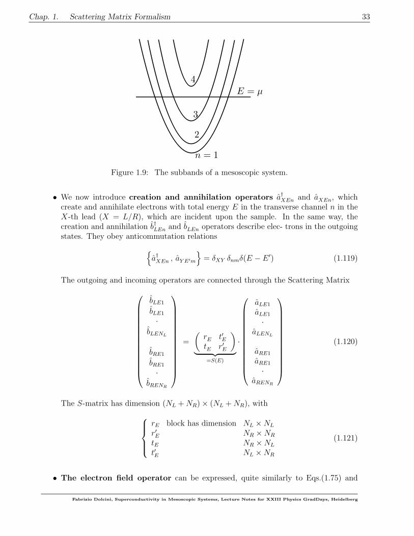
The energies EXn can be viewed as the band bottom of the longitudinal band for the n-thquantum channel in lead X = L/R, as shown in FIg.1.9 Since El ≥ 0, for a given total en-ergy E only a finite number of channels exists. The number of incoming channels is denotedNL(E) in the Left and NR(E) in the Right lead, respectively.
Fabrizio Dolcini, Superconductivity in Mesoscopic Systems, Lecture Notes for XXIII Physics GradDays, Heidelberg
Chap. 1. Scattering Matrix Formalism 33
E = µ
n = 1
3
2
4
Figure 1.9: The subbands of a mesoscopic system.
• We now introduce creation and annihilation operators a†XEn and aXEn, whichcreate and annihilate electrons with total energy E in the transverse channel n in theX-th lead (X = L/R), which are incident upon the sample. In the same way, thecreation and annihilation b†LEn and bLEn operators describe elec- trons in the outgoingstates. They obey anticommutation relations
a†XEn , aY E′m
= δXY δnmδ(E − E ′) (1.119)
The outgoing and incoming operators are connected through the Scattering Matrix
bLE1
bLE1
·bLENL
bRE1
bRE1
·bRENR
=
(rE t′EtE r′E
)︸ ︷︷ ︸
=S(E)
·
aLE1
aLE1
·aLENL
aRE1
aRE1
·aRENR
(1.120)
The S-matrix has dimension (NL +NR)× (NL +NR), withrE block has dimension NL ×NL
r′E NR ×NR
tE NR ×NL
t′E NL ×NR
(1.121)
• The electron field operator can be expressed, quite similarly to Eqs.(1.75) and
Fabrizio Dolcini, Superconductivity in Mesoscopic Systems, Lecture Notes for XXIII Physics GradDays, Heidelberg

34 Multi-channel case
(1.76), as
Ψ(r ∈ L, t) =1√2π~
∫dE e−iEt/~
NL(E)∑n=1
χLn(r⊥)√vn(E)
(eikEnx aLEn + e−ikEnx bLEn
)(1.122)
Ψ(r ∈ R, t) =1√2π~
∫dE e−iEt/~
NR(E)∑n=1
χRn(r⊥)√vn(E)
(e−ikEnx aREn + eikEnx bREn
)(1.123)
where
– kLEn =√
2m(E − EXn)/~
– χXn(r⊥)’s are the transversal wave-function in lead X = L/R, and r⊥ = (y, z) isthe transversal coordinate.
• The electron current operator along the longitudinal direction is obtained by in-tegrating over the transversal coordinates
I(x, t) = −i~ q
2m
∫∫dr⊥
(Ψ†(r, t)
∂Ψ
∂x(r, t)− ∂Ψ†
∂x(r, t)Ψ(r, t)
)(1.124)
In the Left lead:
– Replacing Eq.(1.122) into Eq.(1.124), and exploiting the normalization oftransversal wavefunctions one straightforwardly generalizes Eq.(1.93) to
I(x ∈ L, t) = −i~ q
2m
∫∫dr⊥
(Ψ†(r, t)
∂Ψ
∂x(r, t)− ∂Ψ†
∂x(r, t)Ψ(r, t)
)=
=q
2π~
∫ ∫dE dE ′ ei(E−E
′)t/~NL(E)∑n=1
· (1.125)
·vn(E) + vn(E ′)
2√vLEnvLnE′
[e−i(kEn−kE′n)x a†LEnaLE′n − ei(kLEn−kLE′n)x b†LEnbLE′n+
]+vn(E)− vn(E ′)
2√vn(E)vn(E ′)
[− e−i(kLEn+kE′ )x a†LEnbLE′n + ei(kEn+kE′n)x b†LEnaLE′n
]
– Adopting the linearization approximation one obtains
I(x ∈ L, t) =q
2π~
∫ ∫dE dE ′ ei(E−E
′)t/~NL(E)∑n=1
· (1.126)
·[
e−i(kEn−kE′n)x a†LEnaLE′n − ei(kLEn−kLE′n)x b†LEnbLE′n+]
Fabrizio Dolcini, Superconductivity in Mesoscopic Systems, Lecture Notes for XXIII Physics GradDays, Heidelberg

Chap. 1. Scattering Matrix Formalism 35
– Using the Scattering matrix one expresses the outgoing operators as a functionof the incoming ones, obtaining
I(x ∈ L, t) =q
2π~∑
X,Y=L/R
∫ ∫dEdE ′ei(E−E
′)t/~∑n,m
AXn,Y mL (E,E ′;x) a†XnE aY mE′
(1.127)where we have introduced
A =??????? (1.128)
– The average current can be expressed as
IL = 〈I(x ∈ L, t)〉 =q
2π~
∫dE Tr
[t†(E)t(E)
](fL(E) − fR(E)) (1.129)
where t(E) is the off-diagonal block of the Scattering Matrix. Notice that thetrace implies that the expression does not depend on the basis adopted for thescattering states. For every energy E the matrix t†(E)t(E) can be diagonalized,and its eigenvalues will be denoted by Tn(E)
Tr[t†(E)t(E)
]=∑n
Tn(E) (1.130)
so that the current reads
IL =q
2π~
∫dE
∑n
Tn(E) (fL(E) − fR(E)) (1.131)
Fabrizio Dolcini, Superconductivity in Mesoscopic Systems, Lecture Notes for XXIII Physics GradDays, Heidelberg

36 Multi-channel case
In the Right LeadWe proceed similarly and obtain the same expression
IR =q
2π~
∫dE
∑n
Tn(E) (fL(E) − fR(E)) (1.132)
In conclusion, the Landauer-Buttiker expression for the average current reads
I = IL = IR =q
2π~
∫dE
∑n
Tn(E) (fL(E) − fR(E)) (1.133)
• The linear conductance At zero temperature, the (linear) conductance is easilyobtained from Eq.(1.133) as
G(V = 0) =e2
h
∑n
Tn(εF ) (1.134)
1.9.1 Example: Quantum Point Contact in a Semiconductor2DEG
• A Quantum Point Contact is a narrow constriction in a 2DEG (2-Dimensional ElectronGas). The constriction is created by applying a potential to some top gates, as shownin Figs.1.10 and 1.11
split gate
split gate
In e
lect
rode
In electrode
x
y
Figure 1.10: Top view of a Quantum Point Contact.
• A nice model for a Quantum Point Contact has been proposed by Buttiker [7], whodescribed the potential inducved by the split gates as
V (x, y) = V0 −1
2ω2xx
2 +1
2ω2yy
2 (1.135)
where V0 is the electrostatic potential at the saddle, and ωx,y the strength of thecurvatures.
ELn = ERn = En = V0 + ~ωy(n−1
2) n = 1, 2, . . . (1.136)
Fabrizio Dolcini, Superconductivity in Mesoscopic Systems, Lecture Notes for XXIII Physics GradDays, Heidelberg

Chap. 1. Scattering Matrix Formalism 37
Al0.3 Ga0.7 As (n-doped)
Al0.3 Ga0.7 As (undoped)
Ga As
Ga As
Al0.3 Ga0.7 As (undoped)
barrier
carrier supplier
cap
2DEG
gate gate
Figure 1.11: Side view of the sample (see Ref.[4] p.131-134).
and it can be shown that the transmission coefficients read
Tn(E − V0) =1
1 + e−b(E−En)b = 2π/~ωx (1.137)
which exhibit a ’Fermi-like’ shape, where the ’inverse temperature’ b is given by theenergy spacing ~ωx related to the longitudinal confinement strength. The behavior ofTn(E) is shown in Fig.1.13: each coefficient changes from 0 to 1 within a smoothingenergy of ~ωx, as a function of V0.
Replacing Eq.(1.137) into the expression (1.138) for the conductance, we obtain
G(εF − V0) =e2
h
∑n=1
1
1 + e−b(εF−V0−~ωy(n− 12
))(1.138)
As one can see G exhibits a staircase dependence on V0, where the steps occurs when-ever V0 matches the values V0 = εF − ~ωy(n− 1/2). The height of the steps (plateau-to-plateau) is given by the quantum of conductance.
• This quantization of conductance has been experimentally observed in a series of fa-mous experiments by Van Wees et al. [6] (see Fig.1.14). These experiments representa striking proof of the existence of contact resistance. Furthermore it pointed out therole of transverse modes in transport properties of narrow conductor. The current iscarried by a discrete number of transverse modes. This discreteness is not evidentif the conductor is extremely wide (W λF ), for a small change in W changes thenumber of transverse channels by a large amount
Fabrizio Dolcini, Superconductivity in Mesoscopic Systems, Lecture Notes for XXIII Physics GradDays, Heidelberg

38 Multi-channel case
V (x, y)
xy
Figure 1.12: Potential profile (1.135) for a Quantum Point Contact.
Figure 1.13: Transmission coefficient (1.137) for a Quantum Point Contact.
Fabrizio Dolcini, Superconductivity in Mesoscopic Systems, Lecture Notes for XXIII Physics GradDays, Heidelberg

Chap. 1. Scattering Matrix Formalism 39
Figure 1.14: Experimental results for conductance quantization in a Quantum Point Con-tact, after Ref.[6].
Fabrizio Dolcini, Superconductivity in Mesoscopic Systems, Lecture Notes for XXIII Physics GradDays, Heidelberg

Bibliography
[1] S. Datta, Electronic Transport in Mesoscopic Systems, Cambridge University Press,Cambridge (1995).
[2] S. Datta, Quantum Transport: Atom to Transistor, Cambridge University Press, Cam-bridge (2005).
[3] Y. Imry, Introduction to Mesoscopic Physics, Oxford University Press, New York (1997).
[4] D. K. Ferry, and S. M. Goodnick, Transport in Nanostructures, Cambridge UniversityPress), Cambridge (2009).
[5] Y. Blanter and M. Buttiker, Shot Noise in Mesoscopic Conductors, [ArXiv versioncond-mat/9910158]
Articles
[6] B.J. van Wees et al., Phys. Rev. Lett. 60, 848 (1988); B.J. van Wees et al., Phys. Rev.B 43, 12431 (1991).
[7] M. Buttiker, Phys. Rev. B 41, 7906 (1990).
[8] W. Liang et al., Nature 411, 665 (2001).
40