inﬂuence of interactive stratospheric chemistry on large

Influence of interactive stratospheric chemistryon large-scale air mass exchange in a global

circulation model

T. Orgis(a),∗ S. Brand(a) U. Schwarz(b) D. Handorf(a)

K. Dethloff(a) J. Kurths(c)

May 29, 2009

(a) Alfred-Wegener Institute for Polar and Marine Research - Research Unit Potsdam(b) Center for Dynamics of Complex Systems at the University of Potsdam

(c) Potsdam Institute for Climate Impact Research

Abstract

A new globally uniform Lagrangian transport scheme for large ensembles of passive tracerparticles is presented and applied to wind data from a coupled atmosphere-ocean climate modelthat includes interactive dynamical feedback with stratospheric chemistry. This feedback from thechemistry is found to enhance large-scale meridional air mass exchange in the northern winterstratosphere as well as intrusion of stratospheric air into the troposphere, where both effects aredue to a weakened polar vortex.

Original publication / citation:European Physical Journal Special Topics, vol. 174,doi:10.1140/epjst/e2009-01105-8

1 Introduction

The topic of this study is the analysis of large-scale transport patterns in the atmosphere over seasonaltime scales. Lagrangian trajectory ensembles are the means of choice, especially with the computingresources available today. Indeed, modeling transport of passive air parcels is a task that scalesvery well with distributed/clustered computer architectures (the current de facto standard in highperformance computing) as each subset of trajectories in an ensemble can be computed independentlyof the others.

While e.g. [Sutton 1994] already employed Lagrangian transport on seasonal and global scales,with focus on higher atmospheric layers, the scale of experiments possible today, with some days ofCPU time even on small clusters (below 50 AMD Opteron CPUs), is a different one: Instead of Sutton’sensemble size of around 50, 000 particles, this study deals with many millions of individual particletrajectories from fully three-dimensional computation, using provided horizontal and vertical windcomponents.

Lagrangian trajectories are always only an infinitesimal probing of the “real” air dynamics. Still,increasing the number of probes is a priority to improve coverage of possible transport paths – and

∗Contact via eMail: [email protected]

1

Orgis et al.– Infl. of interactive strat. chem. on air mass exchange

in this case, the actual quantification of air transport and mixing between certain source and targetregions.

The subject to be analyzed for its transport properties is the model data resulting from runs of thecoupled atmosphere-ocean climate model described in [Brand 2008], which incorporates dynamicalfeedback coupling with stratospheric chemistry. The question is: What influence on large-scale air massexchange does the interactive stratospheric chemistry exert?

For assessing that question, the focus is on the change in atmospheric air mass transport from polarregions into lower latitudes and intrusion of stratospheric air into the troposphere. It is investigatedhow the important transport barriers of the polar vortexes and at the tropopause are altered in theimproved general circulation model.

After an introduction to the climate model and the data which was used to compute transport, aswell as a brief discussion of relevant differences in the respective two model runs within section 2,the global transport method itself is presented in section 3. The two main computer experimentsinvestigating changes in large-scale air mass exchange are described in section 4, along with theirresults. Finally, section 5 consists of a summary and conclusions.

2 Data

2.1 ECHO-GiSP: Global circulation model and simulations

Wind data from two long term climate simulations with the coupled AOGCM1 ECHO-GiSP2 havebeen used for the transport experiments in this study. ECHO-GiSP, as described by [Brand 2008],is a development based on the coupled AOGCM ECHO-G [Legutke and Voss 1999]. Essentially, themiddle atmosphere version [Manzini and McFarlane 1998] of the atmospheric model part (ECHAM,[Roeckner et al. 1996]) was used, and in particular the model was also extended by an interactivechemistry module based on the MECCA chemistry module [Sander et al. 2005]. This enables a de-tailed discussion of two way feedback loops between stratospheric chemistry, which is mainly astratospheric ozone chemistry, and atmospheric circulation within a coupled AOGCM.

Technically, there are 39 model levels in the atmosphere, which have been interpolated to 23 pressurelevels between 1000 hPa and 0.01 hPa for the transport computations. Horizontally, a spectral T30resolution has been employed for the atmosphere with 3.75◦ longitude resolution and around 3.7◦ lati-tude resolution in grid space. Furthermore, the ocean-sea ice component (HOPE-G, [Wolff et al. 1997])used 21 vertical levels and a horizontal resolution of T42 with a refinement towards the equator, andfor heat and freshwater exchange between the atmosphere- and the ocean component a flux correctionwas applied.

The ECHO-GiSP interactive chemistry scheme includes mainly gas phase and photolysis reactions,but also heterogeneous reactions on polar stratospheric clouds. On the whole, 39 chemical species and116 reactions were used for the ECHO-GiSP simulations analyzed in this paper. The species includethe main members of the Ox, NOx, ClOx, HOx and BrOx chemical families, as well as gases likeCO, CO2, CH4, N2, H2, H2O. Focusing on stratospheric chemistry, data from the KASIMA chemistrytransport model [Kouker et al. 1999] was used in the troposphere to provide boundary conditionsthere. With this setup, prescribing the chemistry in the troposphere, the scheme is simplified but stillallows interactive chemistry and dynamical feedback in the stratosphere.

Using the described scheme, two long-term simulations of 150 years each were performed astimeslice experiments under fixed present-day conditions. While both of them were fully coupledatmosphere-ocean-sea ice runs including stratospheric chemistry, only their treatment of the trace gasconcentrations within the ECHO-G radiation scheme [Morcrette 1991] differed. The so called coupledrun, denoted as COUP, took into account the interactive chemistry-dynamics coupling, which means

1Atmosphere-Ocean General Circulation Model2ECHO-G with Integrated Stratospheric chemistry by AWI Research Unit Potsdam

2


that the radiation scheme was driven by the simulated stratospheric fields of the chemical constituents.On the other hand, the reference run (REF) used prescribed climatological trace gas fields, so that inthis case the dynamical variables did not depend on the simulated chemistry.

2.2 Dynamical changes

A central structure for global air mass exchange is the polar vortex, being a meridional barrier andforming a dynamical connection between middle atmosphere and troposphere. For the coupled modelrun, a weakened polar vortex has been been diagnosed in [Brand 2007]. The December to February(DJF) mean zonal wind difference for the Northern Hemisphere (NH) winter vortexes of both runs,averaged over the last 120 years, is in the order of 10 m/s. This is about one third of the total windspeed relative to the vortex in the reference simulation. For the Southern Hemisphere (SH) winter,the corresponding absolute wind difference between the modeled vortexes is similar, but because ofthe generally more stable vortex with higher wind speeds, its relative scale is smaller. Therefore, themost significant effects are to be expected for the NH winter.

It is a known fact that many models overestimate the strength of the polar vortex (see, e.g.,[Stenchikov et al. 2006]). In this respect, the consideration of interactive chemistry feedbacks thatreduce the strength of the vortex, is an important step for the further improvement of climate models.

The weakening of the stratospheric polar vortex in the coupled model run is connected with adecrease of the strato-mesospheric residual circulation (Brewer-Dobson circulation) through morestable stratification of the stratosphere. This stabilizing effect in the middle atmosphere can beexplained by a vertical adjustment of the interactive ozone distribution compared to the prescribedprofile in the reference simulation (see upper part of Figure 1). The shifted vertical ozone distribution,especially in lower latitudes, causes more heating at higher altitudes and less heating at lower altitudes(see lower part of Figure 1), leading to an increased stratospheric temperature gradient (see Figure 2),hence more stable stratification.

With a weaker Brewer-Dobson circulation and stratospheric polar vortex, the atmospheric down-welling at the poles, responsible for relatively warm air above, but cold air inside and below the polarvortex, is reduced. Thus, a weaker meridional temperature gradient between pole and tropics evolvesin the troposphere. While first of all, this is associated with a weaker tropospheric zonal mean flow,it also provides better conditions for wave propagation, with the potential to amplify the planetaryand synoptic scale wave activity in mid-latitudes. Due to wave forcing by vertical propagating tropo-spheric planetary waves (see [J.G. Charney, P.G. Drazin 1961]), this again weakens the stratosphericpolar vortex.

The following Lagrangian particle transport investigations shall determine how far the weakenedvortex influences the strength of air mass transport out of polar latitudes and from the stratosphere tothe troposphere. A weaker transport barrier leads to the expectation of increased meridional transportbetween polar and mid latitudes. This could also enhance the deep stratospheric intrusion throughthe extratropical lowermost stratosphere as described in [Stohl et al. 2003].

3 Method

3.1 Transport computation

A global passive tracer transport scheme, working with the wind fields from the ECHO-GiSP modelruns3, has been designed and implemented in form of the computer program package PEP-Tracer(see [Orgis 2007] for a detailed presentation). This scheme uses explicit Lagrangian computation ofindividual test particle trajectories, aggregated to ensembles of millions, to prepare statements aboutthe movement of air masses from the starting regions of the ensembles.

3Generally with gridded longitude/latitude/pressure data in NetCDF format.

3


Figure 1: Zonal mean of the difference between the ozone mixing ratio of the coupled simulationand the fixed ozone mixing ratio in the reference simulation on the top, and on the bottomthe corresponding temperature difference. The temporal mean is computed over the last120 simulation years, DJF. The modified ozone distribution causes according changes in thetemperature field through absorption of short-wave radiation.

4


Figure 2: Global mean temperature profiles for coupled and reference run, mean over the last 120simulation years, DJF. The vertical temperature gradient is enhanced in the coupled run andindicates more stable stratification.

While the wind fields are given in an usual grid with longitude and latitude intervals as horizontaldivision, the actual advection is computed in a local Cartesian coordinate system for each particleand for each time step. This is a different approach than that used e.g. in the standard FLEXTRAtrajectory model [A. Stohl, P. Seibert 1998], where the polar problem is handled by switching to acommon stereographic polar projection above a certain latitude. Here, the coordinate transformationis applied at every location. In addition to eliminating the geometric problem near the poles, this allowsuse of standard time-integration schemes for Cartesian space in a straight-forward way, withoutmodifications.

The local system is a combination of a local orthographic projection4 onto the tangent plane withthe base point B = (λb, ϕb, pb) as the coordinate origin (see Figure 3) and an independent barometrictransformation of the vertical p coordinate5. Any point P(λ,ϕ, p) in the neighborhood of B has thecoordinates P′(x, y, z) in the local Cartesian space (using the radius R = 6370 km):

λ′ = λ − λp −π2

z(p) = 6715m · ln( p101300Pa

)xyz

= R

cosϕ · cosλ′

cosϕ · sinλ′ sinϕp + sinϕ cosϕpz(p)

. (1)

4As usual, the earth is treated as perfect sphere in approximation, with the thickness of the atmosphere being neglectedfor the global geometry.

5This is a modification with respect to the original version presented in [Orgis 2007].

5


x

y φ

RR

θP’

P

Figure 3: Local orthographic projection near the base point B (center of the concentric circles) frompoint P in longitude and latitude to the Cartesian point P′ in x and y. The vertical coordinatereceives separate treatment.

The horizontal velocity is constructed from the wind components u and v using the transformed basevectors ~eu and ~ev:

~eu =

− sinλ′

sinϕp cosλ′

0

, (2)

~ev =

− cosλ′ sinϕ

− sinϕp sinλ′ sinϕ + cosϕp cosϕ0

. (3)

Of course there is some error involved in the chosen local coordinate projection from the curvedsphere to a plane. But this error is not systematically increasing towards the poles, where “south” or“north”, respectively, can mean many different directions, depending on a displacement of the pointof view. The projection error is the same everywhere around the globe, preventing a systematic biason the transport computation based on the spatial region of that transport. Though, in practice onecannot prevent a systematic error from the varying density of grid points where sampled wind datais given.

The grid cells are not projected to proper rectangles and in the case of the inner polar region,the grid cell is actually a polygon with many vertices (96 with the ECHO-GiSP data), due to thelack of defined wind data at the pole itself. Therefore, one cannot use an interpolation algorithmthat depends on a specific regular grid structure. The globally uniform scheme is kept by usingthe flexible Shepard interpolation ([Shepard 1968], also known as distance weighted sum with thedistance function d(~x, ~xi)) in the local Cartesian horizontal plane. With n surrounding grid points atpositions (xi, yi), the value of a quantity u at (x, y) is then given by

u(~x) =

n∑i=1

1d(~x,~xi)k u(~xi)

n∑i=1

1d(~x,~xi)k

. (4)

The exponent for the distance weight was set to k = 2, as determined optimal by [Shepard 1968].In z and time direction simple linear interpolation between the respective values resulting from thehorizontal interpolation is applied.

In the local space with interpolation values for the wind, the trajectory of the particle currently atthe base point B can be computed using several standard algorithms. A four-stage Runge-Kutta as asafe known method has been chosen.

Brief glimpses of the overall advection of air from columns at the poles (extending over the fullheight of the provided wind data) are shown in Figure 4. The advection is computed directly at andaround the poles naturally like anywhere else with the described method.

6


Figure 4: Example column ensembles after 0, 0.2, 0.5, 2, 5 and 10 days for north pole on the top andsouth pole on the bottom, showing characteristic patterns for the respective pole (duringNH winter). Columns over the polar regions, filled with 3,216 particles 1000 hPa to 0.01 hPa,have been advected. The plots show the projection of all particles onto the earth surface,giving a flat view of the horizontal transport dynamics throughout the columns.

7


0

2

4

6

8

10

12

14

16

-80-60-40-20020406080

erro

r/

km

latitude / degN

horizontal forth/back advection error

DecemberJuly

0

2

4

6

8

10

12

-80-60-40-20020406080

erro

r/

m

latitude / degN

vertical forth/back advection error

DecemberJuly

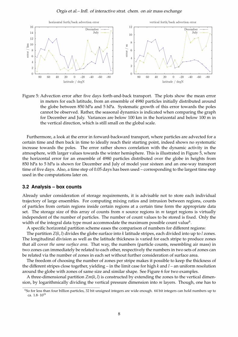
Figure 5: Advection error after five days forth-and-back transport. The plots show the mean errorin meters for each latitude, from an ensemble of 4980 particles initially distributed aroundthe globe between 850 hPa and 5 hPa. Systematic growth of this error towards the polescannot be observed. Rather, the seasonal dynamics is indicated when comparing the graphfor December and July. Variances are below 100 km in the horizontal and below 100 m inthe vertical direction, which is still small on the global scale.

Furthermore, a look at the error in forward-backward transport, where particles are advected for acertain time and then back in time to ideally reach their starting point, indeed shows no systematicincrease towards the poles. The error rather shows correlation with the dynamic activity in theatmosphere, with larger values towards the winter hemisphere. This is illustrated in Figure 5, wherethe horizontal error for an ensemble of 4980 particles distributed over the globe in heights from850 hPa to 5 hPa is shown for December and July of model year sixteen and an one-way transporttime of five days. Also, a time step of 0.05 days has been used – corresponding to the largest time stepused in the computations later on.

3.2 Analysis – box counts

Already under consideration of storage requirements, it is advisable not to store each individualtrajectory of large ensembles. For computing mixing ratios and intrusion between regions, countsof particles from certain regions inside certain regions at a certain time form the appropriate dataset. The storage size of this array of counts from n source regions in m target regions is virtuallyindependent of the number of particles. The number of count values to be stored is fixed. Only thewidth of the integral data type must accommodate the maximum possible count value6.

A specific horizontal partition scheme eases the comparison of numbers for different regions:The partition Z(k, l) divides the globe surface into k latitude stripes, each divided into up to l zones.

The longitudinal division as well as the latitude thickness is varied for each stripe to produce zonesthat all cover the same surface area. That way, the numbers (particle counts, resembling air mass) intwo zones can immediately be related to each other, respectively the numbers in two sets of zones canbe related via the number of zones in each set without further consideration of surface area.

The freedom of choosing the number of zones per stripe makes it possible to keep the thickness ofthe different stripes close together, yielding – in the limit case for high k and l – an uniform resolutionaround the globe with zones of same size and similar shape. See Figure 6 for two examples.

A three-dimensional partition Zm(k, l) is constructed by extending the zones to the vertical dimen-sion, by logarithmically dividing the vertical pressure dimension into m layers. Though, one has to

6So for less than four billion particles, 32 bit unsigned integers are wide enough. 64 bit integers can hold numbers up toca. 1.8 · 1019

8


treat counts of particles from different pressure levels carefully when it comes down to air mass. Theexponential variation of air density with height mandates that one can only directly relate regioncounts from the same level to each other.

4 Experiments

Two experiments with passive tracer particle ensembles have been performed:

1. starting ensembles filling polar columns, throughout tropo- and stratosphere

2. starting ensemble filling a layer around the globe at 10 hPa.

In both cases the ensembles have been advected for winter and summer seasons, the evolution of theparticle distribution indicating the strength of air mass exchange between the starting region and atarget region.

Among the 95 years available out of the 150 modeled years, sample time slices have been chosenfor the transport investigation, disregarding the first decades to account for the model spin-up.

4.1 Polar columns

4.1.1 Setup

From the available data, ten DJF (December to February) and ten JJA (June to August) periods in stepsof five years from years 25/26 up to 70/71 have been chosen. Starting ensembles were created withan horizontally even distribution of 2930 particles per great circle around the north and south poles,in latitudes up to 66.6◦ and 89 pressure levels from 1000 hPa to 1 hPa. With the 112923 particles perlevel, the particle count per column is over 1 · 107 for each pole and season. The experiment is set outto compare the coupled and reference runs of ECHO-GiSP, so, altogether, 2 · 2 · 2 · 10 · 1 · 107

≈ 8 · 108

individual trajectories have been employed. The column ensembles have been advected using thedescribed PEP-Tracer scheme with a time step of 0.05 days (72 Minutes) over the respective three-month period.

4.1.2 Analysis

The trajectories have been sorted into boxes according to Z30(5, 3), limited to latitudes between±66.56◦

and the respective pole, for the source location and Z30(7, 13) for the target location somewhere onthe globe (Figure 6). Based on the counts in these boxes, air mass exchange from the polar region isquantified.

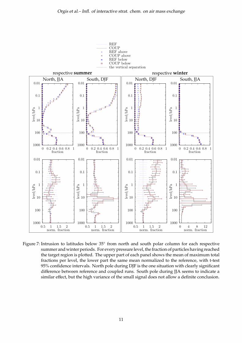
The basic number for each vertical layer is the maximum fraction of the particles having reachedbeyond 35◦N, or 35◦S, respectively, started from the polar region inside 67◦, for the advection periodof three months. The final numeric value is the mean over the maximum fraction for the ten individualperiods.

In addition, the same counting process has been applied to the number of particles having reachedbeyond 35◦ above 100 hPa or below that vertical separation, respectively (called “COUP above”, “REFabove” and “COUP below”, “REF below” in Figure 7). The three resulting graphs give a basic view onthe vertical connection – or lack of – in the polar vortex through 100 hPa together with the horizontaltransport out of the polar regions.

Four comparison plots between the control run and the coupled run summarize the result: Airmass exchange from north or south pole, during respective summer or winter.

In Figure 7, the respective summer season for the concerned pole shows little difference. The graphsfor the coupled and reference run cling close together, hardly showing any significant difference.Generally, there is mixing of polar particles into lower latitudes approaching 80% of the particle

9


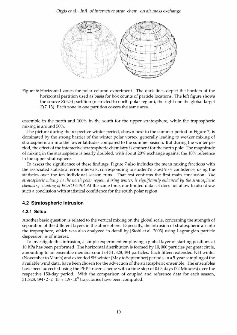
Figure 6: Horizontal zones for polar column experiment. The dark lines depict the borders of thehorizontal partition used as basis for box counts of particle locations. The left figure showsthe source Z(5, 3) partition (restricted to north polar region), the right one the global targetZ(7, 13). Each zone in one partition covers the same area.

ensemble in the north and 100% in the south for the upper stratosphere, while the troposphericmixing is around 50%.

The picture during the respective winter period, shown next to the summer period in Figure 7, isdominated by the strong barrier of the winter polar vortex, generally leading to weaker mixing ofstratospheric air into the lower latitudes compared to the summer season. But during the winter pe-riod, the effect of the interactive stratospheric chemistry is eminent for the north pole: The magnitudeof mixing in the stratosphere is nearly doubled, with about 20% exchange against the 10% referencein the upper stratosphere.

To assess the significance of these findings, Figure 7 also includes the mean mixing fractions withthe associated statistical error intervals, corresponding to student’s t-test 95% confidence, using thestatistics over the ten individual season runs. That test confirms the first main conclusion: Thestratospheric mixing in the north polar region, during winter, is significantly enhanced by the stratosphericchemistry coupling of ECHO-GiSP. At the same time, our limited data set does not allow to also drawsuch a conclusion with statistical confidence for the south polar region.

4.2 Stratospheric intrusion

4.2.1 Setup

Another basic question is related to the vertical mixing on the global scale, concerning the strength ofseparation of the different layers in the atmosphere. Especially, the intrusion of stratospheric air intothe troposphere, which was also analyzed in detail by [Stohl et al. 2003] using Lagrangian particledispersion, is of interest.

To investigate this intrusion, a simple experiment employing a global layer of starting positions at10 hPa has been performed. The horizontal distribution is formed by 10, 000 particles per great circle,amounting to an ensemble member count of 31, 828, 494 particles. Each fifteen extended NH winter(November to March) and extended SH winter (May to September) periods, in a 5-year sampling of theavailable wind data, have been chosen for the advection of the stratospheric ensemble. The ensembleshave been advected using the PEP-Tracer scheme with a time step of 0.05 days (72 Minutes) over therespective 150-day period. With the comparison of coupled and reference data for each season,31, 828, 494 · 2 · 2 · 15 ≈ 1.9 · 109 trajectories have been computed.

10


REFCOUPREF aboveCOUP aboveREF belowCOUP belowthe vertical separation

respective summer respective winterNorth, JJA

0.01

0.1

1

10

100

10000 0.2 0.4 0.6 0.8 1

leve

l/hPa

fraction

0.01

0.1

1

10

100

10000.5 1 1.5 2

leve

l/hPa

norm. fraction

South, DJF0.01

0.1

1

10

100

10000 0.2 0.4 0.6 0.8 1

leve

l/hPa

fraction

0.01

0.1

1

10

100

10000.5 1 1.5 2

leve

l/hPa

norm. fraction

North, DJF0.01

0.1

1

10

100

10000 0.2 0.4 0.6 0.8 1

leve

l/hPa

fraction

0.01

0.1

1

10

100

10000.5 1 1.5 2

leve

l/hPa

norm. fraction

South, JJA0.01

0.1

1

10

100

10000 0.2 0.4 0.6 0.8 1

leve

l/hPa

fraction

0.01

0.1

1

10

100

10000 4 8 12

leve

l/hPa

norm. fraction

Figure 7: Intrusion to latitudes below 35◦ from north and south polar column for each respectivesummer and winter periods. For every pressure level, the fraction of particles having reachedthe target region is plotted. The upper part of each panel shows the mean of maximum totalfractions per level, the lower part the same mean normalized to the reference, with t-test95% confidence intervals. North pole during DJF is the one situation with clearly significantdifference between reference and coupled runs. South pole during JJA seems to indicate asimilar effect, but the high variance of the small signal does not allow a definite conclusion.

11


COUP NH winter after 120d

1e-5 0.001 0.1 1fraction

scale

SN -80-60-40-20020406080latitude

10

100

1000

leve

l/hPa

COUP SH winter after 120d

1e-5 0.001 0.1 1fraction

scale

SN -80-60-40-20020406080latitude

10

100

1000

leve

l/hPa

REF NH winter after 120d

1e-5 0.001 0.1 1fraction

scale

SN -80-60-40-20020406080latitude

10

100

1000

leve

l/hPa

REF SH winter after 120d

1e-5 0.001 0.1 1fraction

scale

SN -80-60-40-20020406080latitude

10

100

1000le

vel/

hPa

Color map: 0 0.1 0.2 0.3 0.4 0.5 0.6 0.7 0.8 0.9 1

Figure 8: Intrusion after 120 days, comparison for coupled run (left) and reference run (right), NHwinter (top), SH winter (bottom). For each of these four subplots, there is on the left side azonal view of the structure of distribution of the stratospheric air being advected, normalizedto the maximum for each level. Right next to this view is a logarithmic graph of the scalevalue for each level and the total fraction of ensemble particles in that level. The overallpattern is essentially identical for the coupled and reference runs, but the generally largeramount of intrusion into lower layers during the NH winter is indicated. More interestingly,the increased intrusion for the coupled model data is apparent.

The purpose of this experiment is to quantify the change in intrusion from the stratosphere into thetroposphere, but also to show how the tracer transport computation reproduces the global circulationpattern.

4.2.2 Analysis

The atmosphere below 10 hPa is the interesting part for this experiment directed at intrusion into thetroposphere. Thus, the target partition is a Z30(10, 60) with 30 levels starting below 10 hPa. Also,when only global vertical exchange is of interest, the source partition can be just one extended region.

This amount of box counts can be visualized to show the distribution of the stratospheric ensembleover time in a zonal projection. The four plots in Figure 8 summarize the four runs (NH/SH winter,coupled/reference) with a snapshot of the distribution after 120 days.

The counts in the partition boxes have been summed along the latitude belts to show the totalfraction of particles from the ensemble being contained in a certain latitude-height region. For thepicture, all the values in one vertical range are normalized to the maximum fraction in that range,amplifying the small values to make easily visible colors but keeping the latitudinal structure. Abar plot next to the pattern visualization shows the fraction that values in a vertical range have beennormalized to as well as the total fraction of the ensemble contained in that vertical range. Together,

12


SH winter (May-Sep)250

300

400

700

800

10000 1 2 3 4 5 6

leve

l/hPa

intrusion, normalized to REF

REF 0.95 conf.COUP 0.95 conf.

REFCOUP

NH winter (Nov-Mar)250

300

400

700

800

10000 1 2 3 4 5 6

leve

l/hPa

intrusion, normalized to REF

REF 0.95 conf.COUP 0.95 conf.

REFCOUP

Figure 9: Ensemble mean global amount of stratospheric air in tropospheric layers between 1000 hPaand 250 hPa after 150 days in comparison for coupled and reference run, SH winter and win-ter. Values are normalized to the reference run, error bars indicate the t-test 95% confidenceintervals. The increased intrusion for NH winter is the most significant signal (at least in theupper troposphere), while the increase for the SH winter is indicated in a similar scale butcloser to the limit of the confidence criterion.

the two sub-plots show the structure and magnitude of the intrusion from the stratosphere into thetroposphere.

The NH winter period of the coupled run (top left of Figure 8) features the general trend todownwelling towards the north that is associated with the stratospheric circulation in northern winter.Concerning intrusion, the main transport path is nicely drawn through the tropopause, at around30◦N. This indicates the mixing through the extratropical lowermost stratosphere as described by[Holton et al. 1995].

Northwards of that, the tropopause shows its strength as a transport barrier: The rectangle from1000 hPa to 200 hPa and from the north pole to 40◦N is basically void of any particles. This is similarfor the southern hemisphere, but generally transport into regions below 200 hPa is channeled throughthe north. For the SH winter period of the coupled run (lower left panel of Figure 8), the situation inthe stratosphere is reversed, with downwelling towards the south pole as a major pattern.

So far this reproduces a global circulation pattern as expected.Superficially, the corresponding plots from the reference run (top and bottom right of Figure 8)

draw the same picture. A difference is in the magnitude of the fractions involved at different heights,observable via the scale graphs. The different strength of intrusion is depicted in detail in Figure 9,with accompanying confidence intervals to evaluate the significance of the difference.

The number of particles, expressed as fraction of the starting ensemble, that reached levels below251 hPa at the end of the advection period, is the final number that is analyzed. The results in Table 1indicate a definite signal from the interactive chemistry: For both seasons, intrusion from the 10 hPastratosphere is around 50% stronger for the advection with ECHO-GiSP data with the interactivelycoupled stratospheric chemistry, compared to the reference without the interactive coupling. The effectis less significant for the SH winter – being subject to larger relative variance, but the main conclusionis: The intrusion of stratospheric air into the troposphere is enhanced by the stratospheric chemistry couplingof ECHO-GiSP.

13


season coupled h reference h coupled/reference

NH winter 0.75 ± 0.17 0.49 ± 0.15 1.5SH winter 0.26 ± 0.08 0.16 ± 0.06 1.6

Table 1: Ensemble mean total intrusion into troposphere below 251 hPa after 150 days expressed interms of fractions of the starting ensemble (ca. 3 · 107 particles), with t-test 95% confidenceintervals.

5 Summary & Conclusions

Using the newly developed and freely available Lagrangian transport software package PEP-Tracer[PEP-Tracer], it is possible to compute reliable three-dimensional global passive tracer transport witha consistent interpolation and integration scheme around the globe, with no exception at the poles.Applying this scheme to wind fields provided by the recently developed ECHO-GiSP AOGCM, theinfluence of the interactively coupled stratospheric chemistry introduced in that model on large-scaletransport between the poles and lower latitudes as well as direct intrusion of stratospheric air into thetroposphere has been analyzed and quantified.

It has been demonstrated that the interactive chemistry coupling of ECHO-GiSP enhances boththe stratospheric air mass exchange from polar latitudes and the intrusion from the extratropicallowermost stratosphere into the troposphere. While the meridional exchange is the primary effect,the intrusion of stratospheric air into the troposphere is mainly a consequence of this. The results ofthe transport study are consistent with the behavior of the polar vortex, which is a main transportbarrier in the stratosphere, in the two analyzed model simulations. The interactive chemistry couplingintroduced in ECHO-GiSP results in a weakened polar vortex, the effect of which on global air masstransport is observable using the PEP-Tracer Lagrangian trajectory method. According to the strongerrelative change in vortex strength for the NH winter, the most significant effects are found for thatperiod, focusing on the northern hemisphere.

Acknowledgments

This work has been funded by the German Helmholtz Association through the Pole-Equator-Polevirtual institute [PEP]. We thank the anonymous reviewers for their helpful comments.

References

[A. Stohl, P. Seibert 1998] A. Stohl, P. Seibert, Q.J. Roy. Met. Soc. 124 (1998), pp. 1465-1484, DOI:10.1002/qj.49712454907

[Brand 2007] S. Brand, K. Dethloff, D. Handorf, Open Atmos. Sci.J. 1 (2007), pp.6-19

[Brand 2008] S. Brand, K. Dethloff, D. Handorf, Geophys. Res. Lett. 35 (2008), pp.L05809, DOI: 10.1029/2007GL032312

[Holton et al. 1995] J.R. Holton, P.H. Haynes, M.E. McIntyre, A.R. Douglass, R.B. Roodand L. Pfister, Reviews of Geophysics 33 (1995), pp. 403-439

[J.G. Charney, P.G. Drazin 1961] J.G. Charney, P.G. Drazin, J. Geophys. Res. 66 (1961), pp. 83-109, DOI:10.1029/JZ066i001p00083

14


[Kouker et al. 1999] W. Kouker, I. Langbein, Th. Reddmann, R. Ruhnke, Wiss. Berichte,FZKA 6278, FZ Karlsruhe, Germany (1999)

[Legutke and Voss 1999] S. Legutke and R. Voss, Technical Report No. 18, ISSN 0940-9327,DKRZ Hamburg, Germany (1999)

[Manzini and McFarlane 1998] E. Manzini, N. A. McFarlan, J. Geophys. Res. 103 (1998), pp. 31523-31540

[Morcrette 1991] J.J. Morcrette, J. Geophys. Res. 96 (1991), pp. 9121-9132

[Orgis 2007] T. Orgis, Lagrangesche Traceradvektion in einem globalen gekoppeltenKlimamodell, http://thomas.orgis.org/diplom/ (2007) (DiplomaThesis, University of Potsdam, Germany)

[PEP] PEP virtual institute, Pole - Equator - Pole (PEP) — Variability ofatmospheric trace constituents along a North-South Transect, http://www.awi-potsdam.de/www-pot/atmo/pep/ (2005-2007)

[PEP-Tracer] T. Orgis, PEP-Tracer software package, http://thomas.orgis.org/pep-tracer/ (2009)

[Roeckner et al. 1996] E. Roeckner, K. Arpe, L. Bengtsson, M. Christoph, M. Claussen,L. Dümenil, M. Esch, M.A. Giorgetta, U. Schlese, U. Schulzweida,Report No. 218, MPI for Met. Hamburg, Germany (1996)

[Sander et al. 2005] R. Sander, A. Kerkweg, P. Jöckel, J. Lelieveld, Atmos. Chem. Phys. 5(2005), pp. 445-450

[Shepard 1968] D. Shepard, A two-dimensional interpolation function for irregularly-spaced data, Proceedings of the 1968 ACM National Conference(1968), pp. 517-524

[Stenchikov et al. 2006] G. Stenchikov, K. Hamilton, R.J. Stouffer, A. Robock, V. Ramaswamy,B. Santer, and H.-F. Graf, J. Geophys. Res. 111 (2006), pp. D07107,DOI: 10.1029/2005JD006286

[Stohl et al. 2003] A. Stohl, H. Wernli, M. Bourqui, C. Forster, P. James, M.A. Liniger, P.Seibert, and M. Sprenger, Bull. Am. Met. Soc. 84 (2003), pp. 1565-1573,DOI: 10.1175/BAMS-84-11-1565

[Sutton 1994] R. Sutton, Q.J. R. Meteorol. Soc. 120 (1994), pp. 1299-1321

[Wolff et al. 1997] J.O. Wolff, E. Maier-Reimer, S. Legutke, Technical Report No. 13,ISSN 0940-9327, DKRZ Hamburg, Germany (1997)

15

http://thomas.orgis.org/diplom/

http://www.awi-potsdam.de/www-pot/atmo/pep/

http://www.awi-potsdam.de/www-pot/atmo/pep/

http://thomas.orgis.org/pep-tracer/

http://thomas.orgis.org/pep-tracer/

inﬂuence of interactive stratospheric chemistry on large

Documents