Inventory Management for an Assembly System

with Product or Component Returns

Gregory A. DeCroix The Fuqua School of Business

Duke University Box 90120

Durham, NC 27708-0120 decroix@mail.duke.edu

Paul H. Zipkin The Fuqua School of Business

Duke University Box 90120

Durham, NC 27708-0120 zipkin@mail.duke.edu

July 2002

Revised December 2003, August 2004, December 2004

Abstract

This paper considers an inventory system with an assembly structure. In addition to uncertain customer demands, the system experiences uncertain returns from customers. Some of the components in the returned products can be recovered and reused, and these units are returned to inventory. Returns complicate the structure of the system, so that the standard approach (based on reduction to an equivalent series system) no longer applies in general. We identify conditions on the item recovery pattern and restrictions on the inventory policy under which an equivalent series system does exist. For the special case where only the end product (or all items used to assemble the end product) are recovered, we show that the system is equivalent to a series system with no policy restrictions. For the general case we explain how and why the system becomes more problematic and propose two heuristic policies. The heuristics are easy to compute and practical to implement, and they perform well in numerical trials. Based on these numerical trials we obtain insights into the impact of various factors, such as the average return rate, return variance, recovery pattern and system structure, on system performance.

1. Introduction

In recent years there has been an increasing need for companies to manage reverse flows

of materials in their supply chains. One reason is the increased frequency with which customers

change their minds and return goods shortly after purchases. Firms have dealt with such returns

for many years, but growth in mail-order and e-business traffic has increased the volume of such

returns — customers unable to see and touch the items they are purchasing are more likely to

return them. (See, for example, Tedeschi 2001.)

Another contributor to the return flow of materials is product take-back — the recovery

of products after customers use them. Due to environmental concerns, several countries legally

require manufacturers to take back certain used products including automobiles, electronic goods

and packaging. (See, for example, Diem, 1999, and Frankel, 1996.) Even when not required to,

some companies voluntarily collect used products from their customers. Examples of such

products include single-use cameras (Kodak, Fuji), toner cartridges (Xerox, Canon, Hewlett-

Packard), personal computers (IBM) and communication network equipment (Lucent). While

this practice may have environmental benefits, the primary incentive is often economic gain —

companies profit from recovering the residual value in the products. In some cases companies

may even design products to maximize this value.

The introduction of uncertain return flows into a supply chain can complicate the

management of the system by increasing variability and thus reducing the precision with which

managers can control inventory levels. The insights and solution methods for traditional

inventory systems (without returns) may no longer apply. Moreover, entirely new research

questions regarding product design, returns network design, returns handling, etc., may arise.

This paper explores the impact on inventory management of introducing returns into an

assembly system — where components are assembled into subassemblies, etc., until a finished

product is produced. These returns may consist of finished goods that can be used immediately to

satisfy new customer demand, or used goods from which components or subassemblies can be

harvested. Our objectives are to develop good policies for managing inventories in this context

and to gain insight into the factors affecting the performance of the system.

Specifically, we analyze an infinite-horizon, periodic-review system with stationary data,

full backordering of unsatisfied demands, and linear holding and backorder costs. We identify

2

two primary ways that returns disrupt the structure of the system, so that the standard approach

(i.e., conversion to an equivalent series system) no longer applies. We identify conditions on the

class of policies and the item-recovery pattern under which these difficulties can be avoided. For

the special cases of recovery of the finished good or recovery of all items used to assemble the

finished good, the assembly system can be reduced to an equivalent series system with no policy

restrictions. As a result, an echelon base-stock policy is optimal, and methods for solving a series

system with returns can be applied. Finally, for a general assembly system without these

conditions, we explain how and why the system becomes more problematic and present two

heuristic methods for computing a good policy. These heuristics perform well in numerical trials.

For a finite-horizon, two-component assembly system, Schmidt and Nahmias (1985)

show that the problem can be decomposed into ordering decisions for the components and an

assembly decision for the finished good (similar to the result of Clark and Scarf 1960 for a series

system). They show, however, that the optimal policy has a complex structure, with the optimal

order for one component depending on the inventory of the other. Rosling (1989) studies a

general assembly system over an infinite horizon. He shows that, under an optimal policy,

inventories in the system satisfy a condition called long-run balance, so that the system can be

reduced to an equivalent series system. As a result, an optimal policy can be computed using the

series-system method of Federgruen and Zipkin (1984) and Chen and Zheng (1994). See Zipkin

(2000) for a more detailed discussion of these results.

For a single-location, finite-horizon inventory system, Heyman and Sobel (1984) point

out that Scarf's (1960) proof of the optimality of an (s,S) policy still works when the system

faces uncertain returns in addition to demands. Fleischmann et al. (2002) extend this result to the

infinite-horizon case. When there is no fixed order cost, a base-stock policy is optimal. Cohen et

al. (1980) establish conditions under which a base-stock policy is optimal when a fixed fraction

of demands in each period is returned after a fixed number of periods. Kelle and Silver (1989)

develop a heuristic approach for managing a similar system that also includes fixed order costs

and stochastic return times.

There has also been research on single-stage systems where returns are not sent directly

to stock (as assumed here) but instead are kept in a separate buffer until they are processed or

disposed of. Simpson (1978) shows that a three-parameter (remanufacture-up-to, order-up-to and

dispose-down-to) policy is optimal for the single-stage, finite-horizon case with linear costs and

3

zero lead times. Inderfurth (1997) extends this result to the case of positive and equal lead times

for delivery of new items and remanufacturing of used items. Mahadevan et al. (2002) develop

heuristic policies for systems with more general lead times.

Research on multi-echelon systems facing product returns has been rather limited.

DeCroix (2001) extends the results of Simpson and Inderfurth to a series system, assuming

disposal is not allowed at downstream stages. For an infinite-horizon series system where returns

go directly to stock, DeCroix et al. (2002) show that an echelon base-stock policy is optimal, and

present exact and approximate methods for evaluating any such policy. The authors also propose

an approximate optimization algorithm for computing a good policy.

For reviews of other research on reverse logistics, see Fleischmann, et al. (1997) and

Dekker, et al. (2004).

This paper extends existing knowledge about management of assembly systems to those

with product or component returns. It also contributes to the recent literature on multi-echelon

inventory systems with returns — particularly by addressing issues, such as recovery of parts of

products and the balancing of component inventories, which do not arise in previous research.

The rest of the paper is organized as follows. Section 2 introduces the model and

notation, while Section 3 explores conditions under which the assembly system is equivalent to a

series system. Section 4 presents a heuristic approach for computing good policies for a general

assembly system, and Section 5 presents the results of a numerical study of that heuristic.

Section 6 provides some concluding remarks.

2. Model

The model builds on that of Rosling (1989), and where possible his notation is used.

Consider an assembly system consisting of items (finished product, components,

subassemblies, etc.) indexed by . Each item has a unique immediate successor,

denoted ) (where , b immediate predecessors denoted

ng that has predecessors requires combining one

unit ea me ate predecesso ecessors are ordered from

outside supplier. There is a lead tim r delivery or assembly of item i . Let )(iA

be the set of all predecessors of item i

illustra such a syste

*** Figure 1 about here ***

N

y have a num

item

i

fo

Ni ,,1K=

and ma

a unit of

rs of

e 1≥il

, and )(iB

m.

i

er of

s without pred

(is

(where })0(P

ch of

tes an

0)1( =s )

.) Assembli

di

i

ple of

)(iP

an

be the

1{=

all im

set of all successors of item

exam

i

. Item

. Figure 1

4

We model time as discrete. In each period t , the system experiences stochastic demand

tD for end items, and stochastic returns tR of end items. A fixed (deterministic) subset J of the

s is recovered from each of the returned units – these items are immediately placed

inventory and can be used to satisfy future demand. (This implicitly assumes 100% reco ry

yield and negligible refurbishment time.) Since we will work with echelon inventor n

is recovered if a return causes that item's echelon inventory to increase. For examp a

ponent is recovered if that comp e is recovered, or if the end product or a

subassembly containing that component is recovered. As a result, if Ji

item

item

com

in

ve

ies, we say a

le,

ny onent alon

r all

led"

(iB

ute

e

j ∈

elem

K

im

s describe

r

nt of past dem

e "m

eans that

d iden

ost assemb

}{i=

y distr

n in so

i

ecov,1{ K=

De

e not r

a

a all ib d.

io mplies that return

∈ then Jj∈ fo

)(iB . For brevity, we sometime J by just referring to th

ents of J . For example, saying that only item is recovered m )J ∪ . Let

JN \}, be the set of items that a ered.

m nds and returns in different periods are independent an tic This

s are independe nds, which is an approximat cases.

One could argue that returns should instead be modeled as a function of past demands. In fact, a

similar issue arises for demand itself. Since no product has an unlimited market, one could argue

that current demand should also depend on past demands. In practice we rarely do that – the

effect is small in most cases, so the added complexity yields little benefit. For similar reasons the

independence assumption is common in the literature on systems with returns. (See Fleischmann

2000 for a more detailed justification of this assumption in that context. Also, see Kiesmueller

and van der Laan 2001 for a single-stage model where returns depend on past demands.) Let

)( tDE=λ , )( tRE=γ , and let )(uD and )(uR be u -period demand and returns, respectively.

Let =M total lead time for item i and all its successors, where 00 =M and

∈ )(iAji ,,1K= dex the items so that 1−≥ ii MM for all i

and i

i

jl for ∑+= ii lM N . (If necessary, re-in

j < f )(iAj∈ .) Also, let 1−or all M max{k=

ii.e., the largest-indexed item

∈J

among

0)(ˆ =ik fo

s successo K∈

iik =)(ˆ . (If 1 , define r all i .) Also, let }J∈: jj =

The system incurs a cost ic for each unit of item i purchased or assembled (due upon

delivery). Shortages of the end item are backordered at a unit cost of p

min{ j be the smallest-indexed

item recovered.

−= iii ML . For Ji∈ , let }:)()(ˆ KkiAik ∈∈ ,

i’ rs that is not recovered, and for define

′ per period, and each

5

unit of item i in inventory or in the process of being cessor item incurs a

(physical) installati H

assembled into its suc

on holding cost of i′ per period. Define the ec

ssors of an item move

must accept all return

helon holding cost as the

(are assembled), i.e.,

∑∈

′−)(iPk

kH . We that the system s, and that the system

it recovery co

additional holding cost incurred when the predece

assume

st of

′=′ ii Hh

incurs a un r f

1

h o ms. Future costs are

discount factor α .

All events occur at the beginning of the peri

g decisi

s are charged. F

e same

ventory pos

f

echelon inventory position of itemons are ma

echelon inventory position of item are ma

echelon inventory on hand of item are ma

11 −+ tR

od in the following or

rs are filled, 4

in a series system. On-ha

stream

t quantity plus ite

variables:

in period t before o

in period t after ord

in period t before o

der: 1) outstanding

rrive, 2) orderin de, 3) backorde customer demands and

ost ollowing standard practice we work with echelon inventory,

lly th nd echelon inventory

ven stage, plus all inventory down of that stage (successor

ition is equal to tha ms that have been

ordered but have not arrived. De ine the following

=itX i rdering/assembly decisi de;

=itY i ering/assembly decisions de;

=litX i rdering/assembly

decisions de, but after orders arrive.

1, −− − ttiit DYX if Ji

orders a

returns o

which h

items

Note that

a

(item i recovered

i (item i not reco

embly decisi

lktX≤ for all Pk

vered), (2)

(dispos wed). so, the a on for each item i is constrained

itY )(i

and itY al is not allo

by the on-hand inventory of its predecessors, i.e.,

Al

∈ , so

+=+−a

aal

ii

RDYRDX if∑−=

t

lt∑−=

− −t

ltalti i, Ji∈ (item i

f Kil

ai

D ∈ (item i not recovered). (4)

We seek a policy (represented by the itY ) that minimizes the expected discounted cost of

operating the system over an infinite horizon.

ed item

or

ons are m

definition here as

)

ccu 5) c

as e entia

is the inventory in stock at a gi

), while echelon in

r,

ss

eac f these ite discounted using a

0 ≤<

= ∈ ), (1)

11, −− − tti DY f i=itX K∈

itX≥ ss

recovered) (3)

i

ttit

∑−

−=− −=

1

,

t

talti

lit i

YX

6

In each period, each item 2≥i incurs physical holding costs on on-hand inventory, i.e.,

( ) ( )[ ]tR iftl

tisttliti DXRDXH +−−+−′ )( i J∈ and is J∈)( ,

( ) ( )[ ]tl

tistliti DXDXH −−−′ )( and Kis ∈)( ,

and ( ) ( )[ ltistt

liti DXRDXH −−+−′ )( n

if Ki∈

]t if Ji∈ a d Kis ∈)( .

Sim sts associated with item 1 are

[ ]ilarly, holding and shortage co

−′ tlt DXH 11 if[ ]−+

+−′++ ttltt RDXpR 1 J∈1 ,

and [ ] [ ]−+ ′+−′ ttlt DXpDXH 111 if −l

t K∈1 .

Finally, the system incurs cost )( iti XYc it − for ordering/assembling units of item i and trR for

recovering returned items.

in period itDecisions in period t affect costs for item i l+ , so we charge period ilt +

costs to period . (Since holding/shortage costs for item iltt, discounted by ilα i in periods ≤

cannot be in ith a

decision, for simplicity we charge those costs to the period in which the returns occur.)

For the cas

fluenced they are omitted. Also, since recovery costs are not associated w

e of K∈1 , summing the cost terms and converting to echelon holding costs

yields a total cost in period

( ) [ ] tttJi

ttliti

Ki

N

iitit

li DXHpRDXhXYc i −′+′++−′++− −

∈∈=∑∑∑ 11

1)()(α .

Now use (1) and (2) to substitute for itX and (3) and (4) to substitute for litX . Taking expected

values, summing over all periods and collecting like term e problem form

Assembly Problem

[ ] [ ] constant)()1(min1

1)1(

11

1 11 +

−′+′+−+′∑ ∑

∞

=

++

=

−

tt

llN

iitii

lt

YYDHpYchE i αααα (5)

subject to

t of

( )tliti DXh −′ rR+

s yields th ulation.

lktitit XYX ≤≤ for all )(iPk ∈ and all i and t . (6)

7

If instead J∈1 , the problem is the same except that [ ]+ − tl YD 1

)1( 1 in (5) becomes

[ ]+++ −− tll YRD 1

)1()1( 11 . The case 1=

+

α corresponds to the average-cost problem. The objective

function is derived by multiplying (5) by αα /)1( − and taking the limit as α goes to 1.

Regardless of whether K∈1 or J∈1 , the constant in (5) is given by

)1/()1/()]1([)1/()]1([ αγααγαααλα −+−+′−−−+′− ∑∈

rlhclhcJi

iiil

iiil ii if <

1∑=

N

i1α ,

and

rlhlhc ii

N

iiii γλ ++′′−∑

=

)]1(([1

if 1=cJi

iγ −−+ ∑∈

[)]1 α . (7)

The cost exp ession in (5) consists of four different categories of costs. In later sections

we will find it conven ent to refer to these categories, so we now.

physical and financi of holding inventory in stock

include holding costs on

it.)

and financial) holding costs of inventory in transit from an

∑ ∑ ∑∑ ∑ ∑∈ ∈ ∪= ∈ ∪

−+′−

−+′Ji iPj

ijPj

iji iPj

ijPj

ij lcHlcH)( )(}{1 )( )(}{

)1()1( γαλα .

purchasing new components and assembling

In any given period the expected

procurement/assembly costs are equal to ∑∑∈=

−Ji

i

N

ii cc γλ

1.

• Recovery costs: The costs of acquiring a returned end product and harvesting usable

items from it. In each period the expected recovery costs are

r

i

Holding/backorder costs: The

y in trans

e cost

define them

al) costs

do not

•

inventor

• Pipelin

(

plus the cost of end-product backorders. (These costs

sical s: The (phy

item to its successor. In any given period the expected pipeline costs are equal to

N

• Procurement/assembly costs: The costs of

components into their successor items.

γr .

To see how these categories relate to the cost expressions above, consider for simplicity

the case 1=α . The constant term (7) clearly contains the procurement/assembly and recovery

costs. Holding/backorder costs and pipeline costs make up the rest of the cost expression in (5).

of backorder costs plus

i holding

costs on that item’s echelon inventory – not on units of item i that have not yet arrived. The

To see this, note that the portion of (5) before the constant term consists

holding costs on echelon inventory position. However, the system only incurs item

8

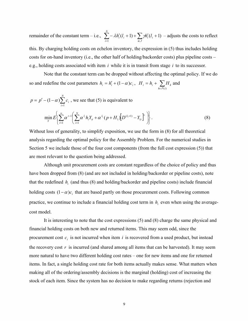
remainder of the constant term – i.e., ∑∑∈=

+′++′−Ji

ii

N

iii lhlh )1()1(

1γλ – adjusts the costs to reflect

this. By charging holding costs on echelon invent (5) thus includes holding

costs for on-hand inventory (i.e., th r costs) plus pipeline costs –

e.g., holding costs associated with item i while it is in transit from stage i to its successor.

Note that the constant term can be dropped without affecting the optimal policy. If we do

so and redefine the cost parameters iii chh )1(

ory, the expression in

e other half of holding/backorde

α−+′= , ∑∈

+=)(iPk

kii HhH and

∑=

−′=N

iicpp

1) , we see that (5) is equivalent to

[ ]

−++∑ ∑

∞

=

++

=

−

11

)1(1

1

1 11 )(t

tll

N

iiti

lt YDHpYhi ααα . (8)

Without loss of generality, to simplify exposition, we use the form in (8) for all theoretical

analys rding the optimal policy f For the numerical studies in

Section 5 w include those of th full cost expression (5)) that

are most relevant to the question being addressed.

Although unit procurem gardless of the choice of policy and thus

have be ped from (8) (and are pipeline costs), note

that the redefined ih (and thus (8) and holding/backorder and pipeline costs) include financial

holding costs ic)1(

−1( α

minY

E

is rega

e

en drop

or the Assembly Problem.

e four cost components (from the

ent costs are constant re

not included in holding/backorder or

α− that are base ollowing common

hen using the average-

) charge the same physical and

ay seem odd, since the

procurem i rom a used product, but instead

the recovery cost

d partly on those

a financial holding cost term in

procurement costs. F

ih even wpractice, we continue to include

cost model.

It is interesting to note that the cost expressions (5) and (8

financial holding costs on both new and returned items. This m

ent cost c is not incurred when item i is recovered f

r is incurred (and shared among all items that can be harvested). It may seem

more natural to have two different holding cost rates – one for new items and one for returned

items. In fact, a single holding cost rate for both items actually makes sense. What matters when

making all of the ordering/assembly decisions is the marginal (holding) cost of increasing the

stock of each item. Since the system has no decision to make regarding returns (rejection and

9

disposal are not allowed), the recovery cost trR is fixed and so r should not become part of the

financial holding cost. On the other hand, if a unit (either new or used) of item i is held in

e period, then that unit of inventory could have been avoided by

ordering one nit of item i at some point in the past, th delaying the procurement cost

ic . In sum, it is logical that both new and used items are charged a financial holding cost of

ic)1(

inventory at the end of som

less unew us

α− .

Assume that the cost parameters satisfy 0>i for all i and 11

)( HphN

i

Mi

is +<∑=

−α . The

latter assump res that it is always optim to fill existing backorders, while the former

reflects higher physical and fina ciated with items that have

progressed farther through the system.

Define µ−MitX to be the echelon i e t of item i ordered

h

al

ncial holding costs typically asso

nventory position at tim

tion assu

i nd product that a

=

, then

, then

≥

∑−

−=

1t

t

−µ −a

,0

µ , ∑−

−=− +=

1

,

t

staa

aasti

Mit RDYX iMs ,,1K= , and

if )(ˆ ik

M<

∑−1t

−µ − ,0

µ−iM periods

ago or earlier. This quantity is an upper bound, based on the current echelon inventory and units

on order of item , on the amount of e could be m de available within µ time

periods. Letting µ−iMs we have:

if Ki∈ −= ,s

astiMit DYX iMs ,,1K= ,

if Ji∈

if )(ˆ ik

M−= st

∑−

+1

aD)µ

aR iMs ,,1,0 K=µ , ∑−−−

−=−=−

− −=1(

,

)(ˆ

µikMt

sta

t

stasti

Mit YX .

This definition adjusts the one in Rosling (1989) to include returns. Note that recovered units of

item i require )(ˆ ik

M periods to be converted into a unit of finished product, so recently

recovered u e been omitted from the expression for µ−MitX in the case of

)nits hav

(ˆ ikM<µ . The

e useful properties of the µ−MitX . following lemma establishes som

10

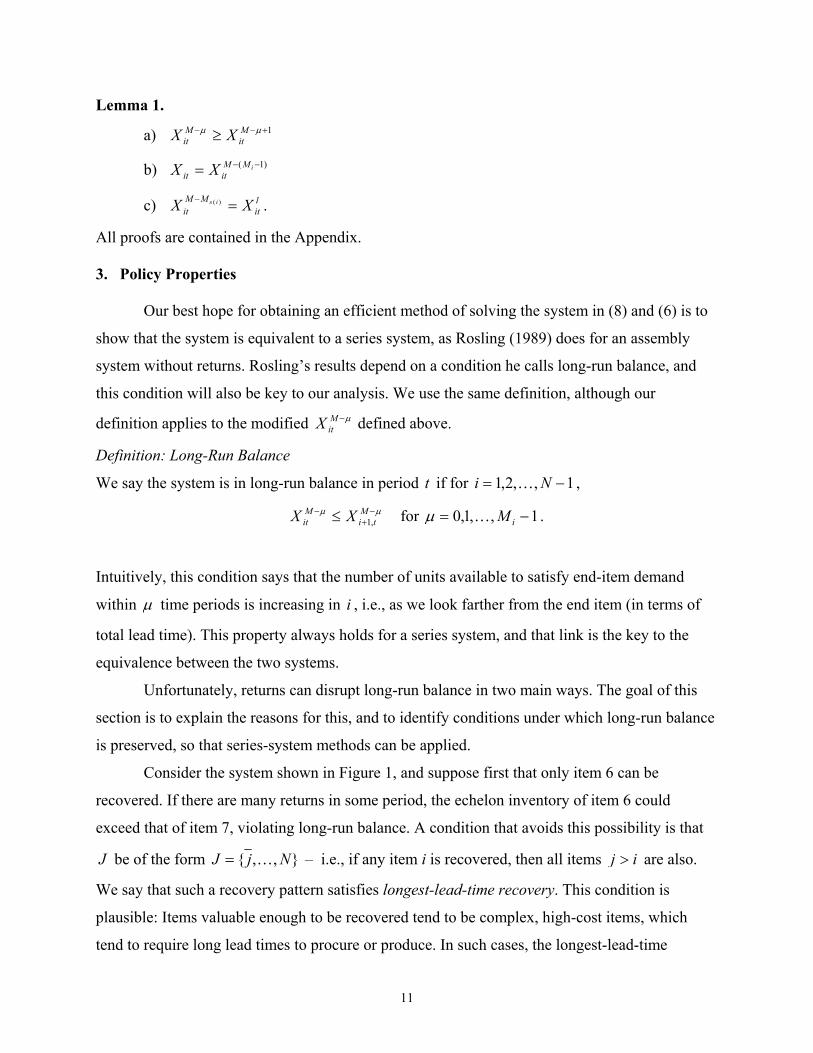
Lemma 1.

a) 1+−≥ µµ MitX

b) )1( −−= iMMitX

c) MitX −

All proofs are contained in the Appendix.

3. Policy Prop

Our best hope for obtaining an efficient method of solving the system in (8) and (6) is to

show that the system is equivalent to a series system, as Rosling (1989) does for an assembly

system ng’s results depend on a condition he calls long-run balance, and

this nditio so be key to our analysis. We use the sam definition, although ou

defin ion ap odified µ−MitX defined above.

Definition: Long-Run Balance

We say the system is in long-run balance in period t if for 1,,2,1

−MitX

itX

lit

M Xis =)( .

erties

without returns. Rosli

n will al

plies to the m

co

it

e r

−= Ni K , µµ −

+− ≤ M

tiMit XX ,1 for 1,,1,0 −= iMKµ .

Intuitively, ays that the number of units available to satisfy end-item demand

within

this condition s

µ time periods is increasing in i , i.e., as we look farther from the end item (in terms of

total lead time). This property always holds for a series system, and that link is the key to the

equivalence between the two systems.

Unfortunately, returns can disrupt long-run balance in two main ways. The goal of this

section is to explain the reasons for this, and to identify conditions under which long-run balance

is preserved, so that series-system methods can be applied.

Consider the system shown in Figure 1, and suppose first that only item 6 can be

recovered. If there are many retu e period, the echelon inventory of item 6 could

exceed that of item 7, violating long-run balance. A condition that avoids this possibility is that

J be of the form

rns in som

},,{ NjJ K= – i.e., if any item ii is recovered, then all items j > are also.

We say that such a recove long . This condition is

plausible: Items valuable enough to be recovered tend to be co lex, high-cost items, which

tend to require long lead times to procure or produce. In such cases, the longest-lead-time

ry pattern satisfies est-lead-time recovery

mp

11

condition may hold. (For example, Toktay et al., 2000, report that the reusable circuit board from

a Kodak single-use camera is the primary cost driver for the product, and that the board is

manufactured overseas resulting in a long delivery lead time.)

Now, suppose that items 5, 6 and 7 are recovered. While this recovery pattern exhibits

longest-lead-time recovery, it may still violate long-run balance. The difficulty here is that

recovered units of item 5 can be converted to finished product more quickly (in 21 ll + periods)

than recovered units of item 6 (which take 31 ll + periods), which could result in µµ −− > Mt

Mt XX 65

for 21 ll +=µ . A condition that avoids this possibility is )1(ˆ)(ˆ +

≥ikik

MM for 1−≤≤ Nij .

One natural type of recovery pattern that satisfies this latter condition we call single-

module recovery odule is recovered (e.g., just item ny

7,,1K )(}{ iBi ∪= ), or if precisely those items requir ssemble a

single module are recovered (e.g., items 2 and 3, or items 4 and 5, or items 6 and 7 in Figure 1).

One interpretation of the latter case is that the module is taken apart into subassemblies and

cleaned or tested before being returned to inventory. Of the single-module recovery patterns, the

ones corresponding to { }7,,1K=J ,

. This holds if just a single m

in Figure 1, so that J

i for a

ed to a=i

{ }7,,2 K=J and { }7,6=J also satisfy longest-lead-time

recovery.

Since the recovery pattern is a function of engineering and design choices, available

recovery technology, etc., nothing in the inventory management policy can prevent the system

from moving out of balance – so analytical results for systems that do not satisf conditions

seem unlikely. We present a heuristic approach for solving such systems in the ection.

Even if the recovery-pattern conditions are satisfied, the optimal orderin

y move the system out of long-run balance. Consid sys

7 is recovered. Wh ding how m 6 t

to anticipate future recovery of item 7. If those returns do not materialize, the system will fall out

of long-run balance. One way to avoid this possibility is to prohibit anticipatory orders – i.e.,

inflated orders of a shorter-lead-tim in anticipation of recovery of a longer-lead-time item.

The definition of non-anticipatory policies can be formalized as follows. Define b to be

the index such that ii MM

ktik

MMbt XX −

>

− = min .

y these

next s

g/asse

der, we

mbly

in Figure 1, and

may try

policy ma

suppose that only item

er again the

uch of item

tem

o oren deci

e item

12

Also, for items Ki∈

} )( iMi

, define the set

{i jJ and)(ˆ jk

M,: BjijJ ≤∉>∈=

non-anticipatory

i

i

MMjtJj

X −

∈min , then itit XY = ;

if itX ≤j

≤ .

(b) If Jbi ∈, and (k̂

M

if itX >

i

i

MMjtJj

X −

∈min

)(ˆ) bkiM> , then

iMMbtX − , then

, then itit YX ≤

itit XY

i

i

MMjtJ

X −

∈min

= ;

itit XYX ≤≤

ple described ab

that item

non-anticipatory policies is s

few constraints. Consider the

. For Jbi

if itX ≤ MMbt

−

Case (a) corresponds to the exam ove, while case (b) addresses the temptation to

order excess of item i is recovered) when another recovered item is closer

to the finished product.

In general the restriction to uboptimal. In some systems,

however, the restriction im system in Figure 1, and suppose

that }7,5,4,2{=J and

iMMbtX − , then

(even though

poses

}6,3,1{=K

i .

∈, it is ea fy that )(ˆ)(ˆ bkik

MM > can never

occur, while for Ki∈

sy to veri

we have ∅= , ,4{31J =J and 7{6 =J

ive to item

act of the non-anticipatory

ing discussion and estab

long-run b

nly limits ord

e explore the

study in Section 5.

bly system

Suppose an assemb

e recovery, and k

M

ers of item 3 (

cost imp

mmarizes the preced

is equivalent to a series system

ly system starts in

)1(ˆ)( +≥

ikiM for 1−≤≤ Ni

.

A policy Y is if it satisfies the following conditions.

Non-Anticipatory Policy

(a) If Ki∈ , then if itX >

}5 }. Thus, the restriction to non-

anticipato policies o relat s 4 and 5) and orders of item 6

(relative to item 7). W ordering restriction as

erical

lishes conditions

under which an assem .

alance, the system experiences

ˆ

ry

part of a num

The following result su

Proposition 1.

longest-lead-tim j . Then under the restriction to

equivalent to a series system with returns at

stage

non-anticipatory policies, the assembly system is

j , the same cost coefficient )( 1Hp + , echelon holding costs iLl hii −α , and lead times iL .

One specific recovery pattern that satisfies the conditions of Proposition 1 is of particular

interest. That is the case where the end product or all of its immediate predecessors are

13

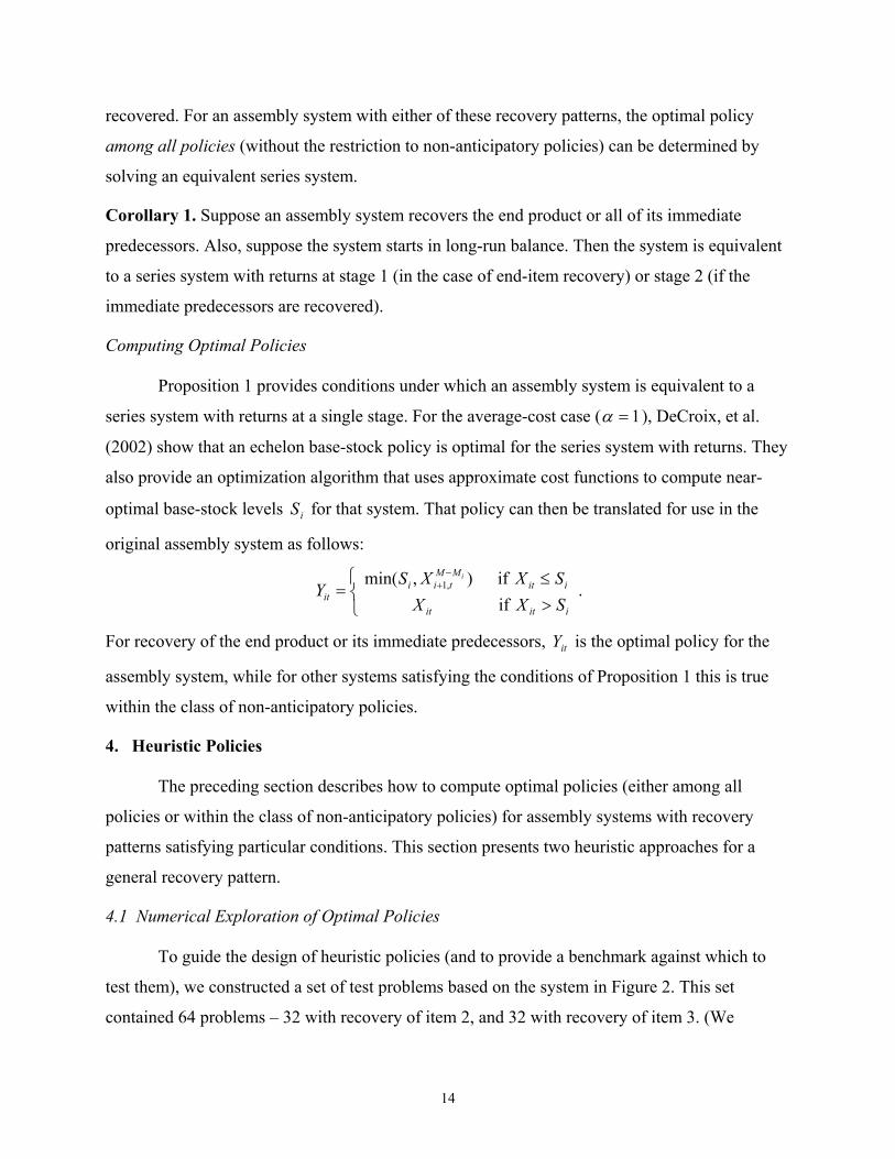
recovered. For an assembly system with either of these recovery patterns, the optimal policy

among all policies (without the restriction to non-anticipatory policies) can be determined by

solv ent .

diate

predecessors. Also, suppose the system starts in long-run balance. Then the system is equivalent

to a series system with returns at stage 1 (in the case of end-item recovery) or stage 2 (if the

immediate predecessors are recovered).

Computing Optimal Policies

Proposition 1 provides conditions under which an assembly system is equivalent to a

series system with returns at a single stage. For the average-cost case ( 1

ing an equival

Corollary 1.

series system

b Suppose an assem ly system recovers the end product or all of its imme

=α ), DeCroix, et al.

(2002) show that an echelon base-sto s op series system with returns. They

also provide an optim t functions to compute near-

optimal base-stock levels iS be translated for use in the

origin sembly system as fo

>≤

=−

+

if if ),min( ,1

iitit

iitMM

tiiit SXX

SXXSY

i

.

For recovery of the end product or its immediate predecessors, itY is the optimal policy for the

assembly system, while for other systems satisfying the conditions of Proposition 1 this is true

within the class of non-anticipatory policies.

4. Heuristic Policies

The preceding section describes how to compute optimal policies (either among all

policies or within the class of non-anticipatory policies) for assembly systems with recovery

patterns satisfying particular conditions. This section presents two heuristic approaches for a

general recovery pattern.

4.1 Numerical Exploration of Optimal Policies

To guide the design of heuristic policies (and to provide a benchmark against which to

test them), we constructed a set of test problems based on the system in Figure 2. This set

contained 64 problems – 32 with recovery of item 2, and 32 with recovery of item 3. (We

ck policy i

ization algorithm that uses

for that system

llows:

timal for the

approximate cos

. That policy can then

al as

14

describe the parame ection 5.) We computed the optimal ordering policy for

each problem by dynamic programming, using the algorithm in Ding et al. (1988), which is a

variation of the policy-iterat

Visual inspection of interesting patterns. A typical

pattern for the case of re

*** Figure 3 about here ***

As defined in Section 2, is the echelon inventory of item 3 ordered one period ago or earlier.

(Here we suppress the time-period subscript t.) From Figure 3 it is easy to see that item 3 follows

an echelon base-stock po ith base-stock level 13. The optimal policy for item 2 is

somewhat more comp 2 follows a type of modified base-stock policy – order up to a

target echelon inventory position *2Y (given any starting echelon inventory position *

212 YX ≤ ),

but that target level chan ith 13X . The policy for item 1 is a base-stock policy, modified as

necessary to reflect availability of items 2 and 3.

Notice that the optimal policy for item 2 exhibits anticipatory ordering. A non-

anticipatory policy would restrict 132 XY ≤ . In Figure 3, however, for low values of 1

3X we have

313

*2 += XY , for me 21

3*

2 += XY , and for high values 16*2 =Y , a constant base-

stock level.

When item 2 is re ered, the optimal policy has some similar patterns, but is a bit more

complex. The optimal *2Y is again a function of 1

3X , but in this case 13

*2 XY ≤ , reflecting

anticipation of recovery of item 2. However, if returns exceed demands for a while, item 2's

echelon inventory 12X may become larger than *

2Y . We observed cases where this effect made it

optimal for item 3’s order to increase – a deviation from a pure base-stock policy. (This

interaction between item nventory and item 3's order never occurs in systems without

returns.)

While the preceding discussion yields some insights regarding the optimal policy, that

policy does not appear to have enough structure to indicate an efficient algorithm. Computing the

optim ic-programming method is feasible for three-item

systems with short lead times and small demand and returns distributions, but not for larger

problems. (A three-item problem with lead times 11

ters in detail in S

covery of

13X

licy, w

lex. Item

ges w

dium values

cov

2's i

ion method of Howard (1960).

the optimal policies revealed some

item 3 is illustrated in Figure 3.

al policy directly using a general dynam

=l , 12 =l and 23 =l , maximum demand of

15

8, and maximum returns of 5 took approximately 32 hours to solve on a desktop PC with a

933Mhz processor. The state space, and thus computation time, grows very rapidly with longer

lead times, larger distributions, and more items.) However, we can use the insights above to

construct tractable heuristics.

ion of Heuristic Pol

We propose two heuristic policies: Heuristic A and Heuristic B. Both are modified base-

stock policies, similar in structure he optimal policy described above. Each policy can be

described by a base-stock level S for each item , and a rule for mo e base-stock policy

based on information about the returns distribu

indexed items. The policies differ in how they ine the base-st s and the

modification rules. H istic A uses just the m the returns distribu ake simple

adjustments to the optimal policy f a system with no returns. Heuristic B is somewhat more

involved, and implicitly ma mation about the entire returns distribution. Concise

specifications of the two heuristic e given below, followed by some illustrative examples.

Heuristic A

Base-stock levels

1. Compute the optimal base-stock levels iS

4.2 Descript icies

to t

i

or

kes use of infor

s ar

de

i =

i M−

i

i

,>kiS

i

,S

i

determ

ean of

difying th

tion and the pipeline inventories of higher-

ock level

tion to meur

′ for the assembly system assuming no returns,

using the techniques of Fe Chen and Zheng (1994). Then

for each item Ki∈ , set iSS

rgruen and Zipkin (1984) and

′

2. For Ji∈ , define )(ˆ iki MN ≡ and set γ⋅−′= iii NSS .

Modification rule

3. For Ki∈ , Jk ∈ and k > , define )(ˆ kkiik MMP −≡ . Then in any period t, the order-up-

to quantity itY for each item K∈ is

}}{min,minmin{,,

γ⋅+= −

∈>

−

∈ ikMM

ktJkik

MMktKkiit PXXY ii . (9)

4. For Ji∈ , Jk ∈ and k , define )(ˆ)(ˆ ikkkik MMQ> −≡ . Then in any period t, the order-

up-to quantity itY for each item Ji∈ is

}}{min},{minmin{,,

γγ ⋅+⋅−= −

∈>

−

∈> ikMM

ktJkikiMM

ktKkikiit QXNXY ii . (10)

16

Step 2 of Heuristic A adjusts the optimal no-returns base-stock levels for each item Ji∈

by the expected amount by which an order for that item will be supplemented as it passes

through the system. For example, for the system in Figure 1, suppose that item 2 is recovered

(i.e., }5,4,2{=J ) and consider an order for item 4. This order will be supplemented by

recovered units until it reaches location 2, i.e., for 314)4(ˆ44 =−=−= MMMMNk

periods, so

we set γ344 −′= SS .

Rosling (1989) shows for a system without returns that the optimal policy uses the

modification rule },{min iMMktiikit XSY −

>′= – i.e., item i's echelon inventory position is constrained

by the pipeline inventories of s. There is no advantage to ordering more,

since those item atche ms farther out in the

pipeline. The m and 4 g reflect returns. Consider again

the example mentioned above. For any pair Kki

higher-indexed item

s would have to wait to be m

odification rules in Steps 3

d with higher-indexed ite

eneralize this to

∈, with ik > , e.g., 6=i and 7=k , Rosling’s

logic still applies, so tha it is always best to restrict }, iMMkti XS − . On the other hand, if

3=i and k K

t

(i.e., i

min{itY ≤

4= ∈ and k ∈ J ) then returns in future periods will supplement the 3

4MM

tX − units currently in item 4’s pipeline. Since those units are 33 =M periods away from the

end item ented by recovery

of item 2 w = M period , item 4’s pipeline will be

supplem

at the tim

hich is

ented by

e an order for item 3 is pla

11 =

)(ˆ

ced, and they are being supplem

away from the end item

21

)4(ˆMk

3 =−=− Mi returns. So for Ki∈ and Jk≡ MPik M periods of Mkk

∈ ,

Step 3 includes the restriction

If 4=i and 6=k in our example (i.e., Ji

γ⋅+≤ −ik

MMktit PXY i .

∈ and Kk ∈ ) then an order for item 4 is

supplemented by 314)(ˆ =−=−≡ MMMMNikii periods of returns on its path to the end item,

while item 6 receives no supplement. So for Ji∈ and Kk ∈ , Step 4 includes the restriction

}γ⋅−≤ −i

Mit NY i . Finally, suppose we modify our example so that item 7 is also

}7,5,4,2{= ). If 4=i and 7

,min{ Mkti XS

recovered (i.e., J (i.e., Ji∈ and Jk ∈ ), then an ord

periods on its path to the end item, while the

e

3)4(ˆ4 =−

kMM 4

7MM

tX −

currently in item 7’s pipeline are supplemented for 134)7(ˆ4 =

r for item

units 4 is supplemented for

=k

−=− MMMMk

period. As a

17

result, item 4 is recovered for 213)(ˆ)(ˆ =−=−≡ MMMMQikkkik more periods than item 7. So

for Ji∈ and Jk ∈ , Step 4 includes the restriction γ⋅−≤ −ik

MMktit QXY i .

Heuristic B is similar in spirit to Heuristi e pute the

base-stock levels and modification rule.

Heuristic B

For , set i′

For , define }{) i∈≡ a su ork of the

essors ))(i and

pr s

c A, but uses a different m

}. No

and all of

thod to com

b-netw~(kA

Base-stock levels

Ki∈

Ji∈

original as

edeces

1.

2.

i SS =

(~ ik

bly system

))(

as in Heuristic A.

min{k

consisting o

:)( kiA∪

f item k

J∈ w con

)(~ i

struct

its succsem

ors ~( ikB . (Note that all elements of ))(~( ik

ly system

B will

mb

also b

is equiv

e

e a e

el

le

ements of

nt to a s

J .) The

ries r sults of

system

Section 3 impl

with returns arriv

y that th

ing at s

is s

tage

maller asse

)(~ ik . Compute the optimal base e-stock lev ls iS ′′ for

acthis system us aping the

))(

proach of DeCroix, et al. (2002). Then for e h ~()}(~{ ik∈ ik ,B∪ set i ii SS ′′=

i> , cho

.

ose

Modification rule

Ki∈3. , k kJ∈ and an adjustmen tity Vt quan iMMkt

−itik Y≡ X− such that

{ } β=≥ikV )( ikP for soR me 0 1<< β (or, if the s distrreturn ibution e, is discret choose

t e sm ik such that V { } β≥)( ikP

,k

MMktX i

>

−

iik NU

≥ R

Y is

min, Kki ∈

Pr ikV

Ki∈

,kiS>

i> , define

). Then in any period

{min, Jki

Vi +∈

t

}}ik .

, the order-up-to

quantity

Ji∈

it for

min{

, k ∈ k

each item

itY =

K and

MMktX −

4. ≡ , and for Ji∈ , Jk ∈ and ik > , define

ikik Q≡U . If and Jk ∈ 0≤ikQ , choose an adjustment quantity ikV such that

{ } β=≥ikV )( ikU for soPr R me 0 1<< β . Otherwise choose an adjustment quantity ikV

(<0) such that { } β=−≥ ikVUik )R (Pr for some 0 1<< β . Then in any period t, the order-

up-to quantity itY for each item Ji∈ is

{min,ikiS

>}}MM

ktX − . min{ ikVi +itY =

For

Pr

h allest

For

18

To illustra

e

te Heuristic B, consider the system

ine the base-stock levels for items , Step 2 comp

to match all

al base-stock levels for the series system

nt quantity ikV in Steps 3 and 4 is chosen so

der for item i arrives, there will be enough un

bility

turns to stag

The adjustm

rrent o

k w

e 3.

e

ith proba

s)

β , i.e., +−Pr{ )( )(ˆ iki MM

it RY

β=− }))(ˆ iki M . The different cases in

β=} , or +−− )( )(ˆ kkii

MMM R

Pr{ ikV s 3 and 4 provide alternate

(simpler) versions of this expression, depending on whether item i or item k is supplemented by

more perio or e ple, if 2

≥ MktX

Step−(MR≥

)( )R − (ˆ kki MM

in Figure 1 and suppose that items 3 and 4

are recover d. To determ }7,6,4,3{=∈ Ji utes

the optim s 4–2–1 with returns to stage 4 and 7–6–3–1

with re

that (adjusting for return

when the cu r its of that item

units of item

ds of returns. F xam and Jk ∈ ), then

can order item 2 up to

es ≥Pr{ )(23

23PRV

item 3 will

be sup the quantity

of item 3 in the pipeline plus a positive adjustm 023 > that solv β=} .

Suppos an

plem 1

e in

ented b

stead th

y 23 =P

at 3=i

period of returns. Therefore we

(i.e., i

ent V

4 Jd =k ∈ and 3 will be sup

s for 1=−=M−k

re period than order item

3 up to the quantity of ite 034 < that solves

β==≥ }Pr{}Pr{ ))( 3434R QU

= M MMQ mo item 4, so we can

=i and 3=k (i.e., Ki∈

Jk ∈ ). Then item plemented

by return 12ˆˆ34 )3()4( k

m 4 in the pipeline plus a negative adjustment V

−≥ 34)1( VR−≥ 34V= Pr{ (R− }34V . The parameter

merical studies in Sec ion 5 use /( ihpp ′+=β , the critical fractile for the newsvendor

entially

re exte

number

problem (relative to item ) resulted in a backord

requir he effo

com o siv puta s

se ystems with

returns. For Heuristic A, com with the modification rules in

Steps 3 and 4 involves only a few simple com ations. For Heuristic B these steps are again

somewhat more involved, but they only require constructing the multi-period returns

distributions and computing the appropriate fractile plementation of the

policy requires the same kind of pipeline information as in an assembly system without returns.

However, since returns can disrupt long-run balance, it is necessary to track the pipeline

that would result if a shortage of item

vel

i

r Heuristic A

stem with

in addition we must solve som

k

es ess

ns. M

e

er.

rt as

tion

Com

puting the optim

are required for Heuristic B, since

puting the base-s

al le

tock

for a s

levels f

eries

o

sy

t

n

of

same

e com

ries s

s out retur

β is user-specified.

The nu t )

puting the parameters associated

put

s. For both heuristics, im

19

inventory of all higher-indexed items when placing an order. (Rosling 1989 shows that, without

returns, when ordering item i cessary to check the pipeline of item 1+i only.)

Num rical studies (discussed in th or

Heuristic B m yield lower ho hile

better than the

pute the costs of ith the

res ption of

istics can b ry pattern

m i

i

, it is ne

oac

tical

ur

rand

and

e

ay

other, a third option is to com

e

ery

(e.

=

e next section) reveal that either Heuristic A

ding/backorder costs, depending on system parameters. W

when one heuristic might be expected to perform

both heuristic policies and use the one w

as the combined heuristic.

ults of the preceding section depend on the assum

e generalized to settings where the recove

recovery yields). To that end, let =iR units of

)( iRE

l

r

e

0

those studies shed some light on

lower cost. W refer to this app h

Finally, while the theore

a fixed recov pattern, both h

is stochastic g., systems with o

recovered, })0Pr(:{ >>iRiJ

item

=γ . (Note that the iR may or may not be

tock levels for Jicorre euristic Alated.) Then for H , the base-s ∈ become iii NSS iγ⋅−′=

(9) and (10): kikik PP

. Also,

the following modifications are e mad in γγ ⋅→⋅ in (9); iN iiN γγ ⋅→⋅

kkk

and iikiik MMQ iM M γγγ ))(ˆ in (10).

odify Step 2, solving a smaller series system consisting

to the end item. The modification rules are determ

, but now they are based on the iR , i.e., choose

())(ˆ −−−→⋅

For Heuristic B, for each Ji∈

just )(iAi ∪ , i.e., the path from

using logic similar to that above

(

we m

item

of

ined

iMMktitik XYV −−≡ so that β=+≥+

−−− }Pr{ )()( )(ˆ)(ˆ kkiiiki MMk

MMkt

MMiit RXRY , or equivalently,

β=−≥−− }Pr{ )()( )(ˆ)(ˆ ikikki MM

iMM

kik RRV . In Section 5.1 we report results of a numerical test of the

heuristics in this more general setting.

5. Numerical Study

In this section we present a two-part numerical study. The first part focuses on small

problems for which the optimal policy can be computed. Here we explore three questions: 1)

How well do the heuristic policies perform relative to the optimal policy and a naïve policy (i.e.,

the optimal policy assuming no returns, but applying it, naively, to the system that does

experience returns)? 2) How do returns affect holding/backorder costs? and 3) How do factors

such as the expected returns, the variance of returns, and the recovery pattern affect system

performance and the performance of the heuristics?

i

20

The second part of the study considers larger problems for which it is impractical to

compute the optimal policy. Here we explore system behavior using only the combined heuristic

policy. We compare holding/backorder costs under that policy to two benchmarks –

holding/backorder costs for a system without returns, and holding/backorder costs for a system

with returns under the naïve policy that ignores returns. We also explore how different

component recovery patterns and system structures affect system behavio conclude with

some com rest stem to non-an pato icies.

n av

interpre

initially fo e e q e p

heu e polic

since these are the only costs that can be influenced by the ordering policy. For other questions

(e.g., the cost impact of increasing the average return rate), these are the only costs that require

involved calculations to com ute – the other three cost components can be easily computed using

essions in Section 3. We ew examples to illus te the impact of these factors

r three cost

ing/Ba

cy performance using

the 64 three-item problems mentioned in Section 4. Specifically, we consider two recovery

patterns – recovery of item 2 only, and recovery of item 3 only. (Note that the other two possible

recovery patterns for this system – recovery of items 2 and 3, or recovery of item 1 – satisfy the

conditions of Corollary 1. As a result, the methods of DeCroix et al. 2002 can be used to

compute the optimal policy, so there is no need to use the heuristic policies.) For each recovery

pattern we considere 32 problems by setting the echelon inventory holding costs ( )321 ,, hhh to

(1,1,1), (4,1,1), (1,4,1) and (1,1,4), the unit backorder cost 10

r. We

ry pol

er-period, but following common practice we

erfor

ly c

ments about the cost of

In both studies we focus o

t the unit holding costs ih

cus on holding/backord

olicies relative to the op

ricting the sy

erage-cost-p

r costs. For som

al and naïv

tici

.g.,

to include both physical and financial components. W

ons (e

ies) thes

e

mance of the

osts that m

uesti th

e are the onristic p tim atter,

p

compo

ckorde

the expr

on these othe

Optimal

We

provide a f

.

t a

tra

ce

isti

nents

r Cos nd Heuristic Performan

al holding/backorder cost and heur c poli

5.1 Hold

investigate optim

=p , and using the 8

demand/returns distributions in Table 1. In all cases returns in a period are independent of

demand in that period.

21

Demand Returns Case 1 D = {0,1,2,3,4,5,6,7,8}

Prob = {0.04,0.08,0.12,0.16,0.2,0.16,0.12,0.08,0.04} E(D) = 4, var(D) = 4

R = {0,1,2} Prob = {0.2,0.6,0.2} E(R) = 1, var(R) = 0.4

Case 2 Same as Case 1 R = {1,2,3} Prob = {0.2,0.6,0.2} E(R) = 2, var(R) = 0.4

Case 3 Same as Case 1 R = {2,3,4} Prob = {0.2,0.6,0.2} E(R) = 3, var(R) = 0.4

Case 4 Same as e 1 R = {0,1,2,3,4} Prob = {0.1,0.2,0.4,0.2,0.1} E(R) = 2, var(R) = 1.2

Cas

Case 5 Same as Case 1 R = {0,1,2,3,4} Prob = {0.2,0.2,0.2,0.2,0.2} E(R) = 2, var(R) = 2

Case 6 Same as Case 1 R = {0,1,2,3,4} Prob = {0.3,0.15,0.1,0.15,0.3} E(R) = 2, var(R) = 2.7

Case 7 Same as Case 1 R = {0,1,2,3,4,5,6,7} Prob = {0.002,0.405,0.306,0.207,0.058,0.008,0.008,0.006} E(R) = 2, var(R) = 1.2

Case 8 D = {1,2,3,4,5,6,7,8} Prob = {0.055,0.25,0.18,0.14,0.12,0.103,0.09,0.062} E(D) = 4, var(D) = 4

R = {0,1,2,3,4} Prob = {0.1,0.2,0.4,0.2,0.1} E(R) = 2, var(R) = 1.2

Table 1

Note that cases 1 through 3 represent increasing mean return rates while return variance is held

constant. Cases 2 and 4 through 6 represent increasing return variability while holding the mean

return rate constant. Case 7 represents a skewed return distribution, while case 8 represents a

skewed demand distribution.

For each of the 64 test problems, we compute expected holding/backorder cost per period

for both heuristic policies and the naïve policy using successive approximations, and then

compare those to the holding/backorder cost of the optimal policy computed by dynam

programming as described in Section 4. Performance is measured by the relative error

Relative Error = (Avg. cost of heuristic) – (Avg. cost of optimal policy)

ic

. (Avg. cost of optimal policy)

Both heuristic policies perform well relative to the true optimal policy – the average

relative errors across all 64 test problems were 1.46% for Heuristic A and 1.65% for Heuristic B.

For Heuristic A, the average relative error was smaller for recovery of item 3 (1.22%) than for

recovery of item 2 (1.70%), while the opposite held for Heuristic B (2.23% for item 3 vs. 1.068%

for item 2). The maximum error was 8.70% for Heuristic A and 6.08% for Heuristic B. By

22

comparison, the naïve policy performs relatively poorly, yielding an average relative error across

the 64 test problems of 10.72% and a maximum error of 44.23%

For two-tier systems consisting of just the end product and a set of components (like the

test problems considered here), it is possible to theoretically address the second question by

comparing the optimal holding/backorder costs for a system with recovery of some of the

components to that of a system without returns. The following result provides such a

comparison.

Proposition 2. If },,2{)1( NP K= , then the optimal holding/backorder cost for the system

without returns is a lower bound for the optimal holding/backorder cost of a system with returns

and any recovery pattern satisfying },,2{ NJ K⊆ .

In order to explore the magnitude of the cost difference identified in Proposition 2, for

each of our 64 test problems we compare the holding/backorder cost under the optimal policy to

the optimal holding/backorder cost for the same system without returns. On average introducing

returns increased optimal holding/backorder costs by 23.4%, with a range of 6.3% to 63.2%. For

Heuristic A (B) the average increase was 25.3% (25.5%), with a range of 6.4% to 68.4% (6.3%

to 63.2%).

Note that if the end item is recovered, returns may result in either higher or lower

holding/backorder costs. For example, if demand and returns in a given period are independent,

then returns cause the average (net) demand for each item in the system to be lower, but the

variance of (net) demand to be higher. This increased variance can make it harder to match

supply with demand, resulting in higher holding/backorder costs. (This can occur even if

1)Pr( => RD , i.e., when net demand is always nonnegative.) On the other hand, if demand and

returns in a given period are correlated, returns may reduce (net) demand variance, yielding

lower holding/backorder costs.

The third question explores the impact of higher return rates or higher return variance.

Figure 4 illustrates the impact of higher average returns when item 3 is recovered and

( ) )1,1,1(,, 321 =hhh . (The graphs for recovery of item 2 and the other holding cost values are

similar.) The figure shows the effect of the return rate on the optimal policy, both proposed

heuristics, and also the naïve policy.

23

*** Figure 4 about here ***

As )(RE increases from 1 to 3.75 with )(DE fixed at 4 (i.e., demand/returns

distribution cases 1 through 3, supplemented by two additional cases with 5.3)( =RE and

75.3)( =RE to explore behavior as )(RE approaches )(DE ), holding/backorder costs increase

at an increasing rate. The absolute and relative heuristic errors tend to grow as )(RE increases,

but there are some exceptions to this pattern. However, even for very high return rates – nearly

94% – both heuristics still perform reasonably well. In that case the average relative error for

Heuristic A is 5.0% when item 2 is recovered and 2.3% when item 3 is recovered, while for

Heuristic B the erro 3.6%, respectively. Note also that the cost advantage of both

heuristics over the n ows with )(RE . In fact, when 75.3)(

rs are 5.7% and

aïve policy gr

rs of 20.3% (item 2

=RE the naïve policy

yields average erro recovered) and 72.9% (item 3 recovered).

With the insights from Figure 4, it is easy to determine how )(RE affects total system

costs in any given situation. Recall that the sum of procurement/assembly, pipeline and recovery

costs is linear in )(RE . If the slope of this sum is positive, then more returns will always lead to

higher total system costs. This would be the case, for example, if returns consist of recently

purchased (new) products, where customers receive a full refund of the retail price. The recovery

cost would then equal the retail price plus any additional costs of cleaning/testing/restocking the

item. Since profitability requires that the retail price is greater than the sum of the pipeline and

procurement/assembly costs associated with producing a single unit, the slope of the linear term

must be positive.

If instead the slope is negative (which may occur if little or no payment is made for the

returned product and usable items can be harvested at sufficiently low cost), then a higher return

ce total system costs at first. However, if as the return rate rises the slope of the

holding/backorder cost curve in Figure 4 becomes equal to the negative of the slope of the linear

term, then any further increase in the return rate would increase total system costs. Figures 5a

and 5b illustrate this relationship between )(RE and total system costs for two sets of examples.

Both figures are based on the same recovery structure (i.e., item 3 is recovered), holding costs,

tions as depicted in Figure 4. In addition we assume unit

procurement/assembly costs of 30=ic for both components and the finished product. Figure 5a

depicts a unit recovery cost of 217.0 3

rate will redu

and sequence of returns distribu

=⋅= cr , while Figure 5b depicts a unit recovery cost of

279.0 3 =⋅= cr . (For simplicity, both figures show the combined heuristic – the better of

24

Heuristics A and B – rather than graphing them separately.) In Figure 5a, a higher return rate

continue l system costs for the entir range of exam

turns start to incre tal sy costs once the return es beyond

a

e lower than with no return agn

e examples, when 9.

e

stem

273

s to reduce tota

about 75% of average dem

onents in thes

ples considered. In contrast, in

rate go

tal system costs with

itudes of the four cost

Figure 5b higher re

returns ar

comp

ase to

nd. Even at these high

s. To give

0

er rates, however, to

a sense of the relative m

=⋅= c 75% of ptimal

holding/backorder cost is 19.2, pipeline cost is 8, t cost is 270, y cost is

** res 5 t here ***

Building on this comp at influence

when a higher return rate is beneficial. If material and labor cost savings on recovered items are

large (i.e., rcJi

i −∑∈

is large), then these savings would tend to outweigh any additional

holding/backorder costs associated with the additional returns. On t r hand, a large unit

backorder cost

r

* Figu

arison, it is stra

and E(R) is

en

b abou

rward to iden

E(D), the o

and recover

actors th

procurem

a and 5

o

81.

ightf tify the f

he othe

p would tend to yield the opposite result. Large uni ng costs ih could

result in either outcome. On the one hand, they would amplify the rate at which higher returns

increase holding/shortage costs. At the same time, however, they could also increase the amount

of pipeline-cost savings resulting from returned items. The net effect would depend on the

specific setting in question. (For example, in the settings in Figures 5a and 5b pipeline costs are

only incurred in transit to item 1, so the return rate has no impact on these costs. As a result,

higher values of ih would only increase the holding/shortage costs.)

Note in Figures 5a and 5b that, not only does the naïve policy yield higher costs than the

combined heuristic, but it also sends misleading signals regarding the profitability of higher

return rates. In Figure 5a the naïve policy suggests that increasing the return rate beyond about

87% of average demand would lead to increased total system costs, while in Figure 5b that cutoff

point is around 50%. In fact, in the latter case, the naïve policy suggests that a return rate above

about 70-75% is actually more costly than no returns. Since the combined heuristic tracks the

optimal cost function much more closely, it provides a much more accurate assessment of returns

profitability.

Figure 6 shows the im ce when item 3 is recovered,

( ) )1,1,1(,, 321 =hhh , )(DE is fixed at 2, and the coefficient of variation

t holdi

pact of return

is fixed at 4,

s varian

)(RE

25

increases from 0.32 to 1.53 (i.e., demand/returns distribution cases 2 and 4 through 6,

ented by an additional case with 4.9)var(supplem

variance increases, the o

A tends to perf

high-variance cases. Th

heuristics are specif

compute the base-s

somewhat, introduc

distortion causes la

(Attempts to ide

introduce this kind of distortion

When returns varian

it does not ma

high-variance case is 6.2

6.78% when item

gains by ma

associated with th

for Heuristic

item 3 is reco

variance of returns incre

are optima

attractive (w

policy parame

Since return

always redu

procurement/assem

bsystems

istic B distorts the

rom optim

euristic A, which is bas

istics th

did not yield any heuristics with

ance o

rmation. The av

ve

ith a worst case of 13.92%).

ation when variance

ws it to outperfo

ase is 0.60%

performanc

ring returns, this po

ered. Since gr

s are larger than ho

s varian

*** Figure 6 about here ***

es not affect the other th

ess of product recove

a

sts. For retu

gher vari

=R to explore behavior with high variance).

(Again, the graphs for recovery of item 2 and for other holding costs are similar.) As returns

ptimal holding/backorder costs increase at a nearly linear rate. Heuristic

orm better when the returns variance is low, while Heuristic B performs better in

is relative performance pattern makes sense given the way the two

ied. By solving su (rather than the entire assembly system) to

tock levels, Heur structure of the assembly system

ing some deviations f ality. When returns variance is low, this

rger errors than H ed on the original assembly system.

ntify alternative heur at incorporate variance information but do not

stronger overall performance.)

ce is very high, the perform f Heuristic A deteriorates somewhat since

ke use of variance info erage relative error for that heuristic in the

3% when item 2 is reco red (with a worst case error of 14.57%) and

3 is recovered (w The advantage tha euristic B

king use of that inform is high outweighs the distor ns

at heuristic, and allo rm Heuristic A. r

h-variance c when item 2 is recovered and 1.95% when

terestingly, the e of the naïve policy appears to improve as the

ases. By igno licy uses higher base-stock levels than

s are consid eater variability makes higher ba -stock levels

hen unit backorder cost lding costs as is the case he the naïve

ters are not as far off when return ce is high.

s variance do ree cost components, higher variance

ces the attractiven ry in terms of total system costs. At some

point, the higher holding/shortage costs m y outweigh any net savings associated with

bly, pipeline and recovery co rns variances up to that threshold

level, recovery is attractive, but at hi ance levels it would actually be better to not

t H

tio

The average relative erro

se

re),

B in the hig

vered. In

l when return

26

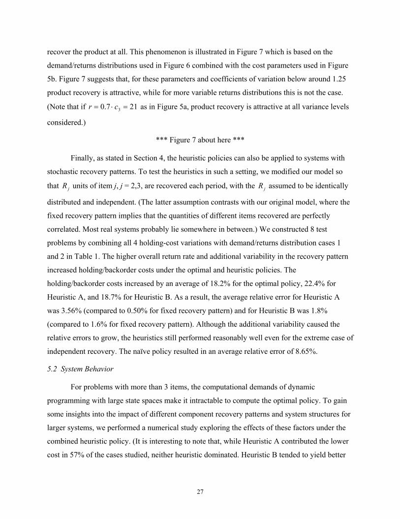
recover the product at all. This phenomenon is illustrated in Figure 7 which is based on the

mbined with the cost parameters used in Figure

, for these pa and coefficients of variation below around 1.25

able returns distributions this is not the case.

(Note that if 217.0 3 =⋅= cr as in Figure 5a, product recovery is attractive at all variance levels

considered.)

*** Figure 7 about here ***

Finally, as stated in Section 4, the heuristic policies can also be applied to systems with

stochastic recovery patterns. To test the heuristics in such a setting, we modified our model so

that jR units of item j, j = 2,3, are recovered each period, with the jR assumed to be identically

distributed and independent. (The latter assumption contrasts with our original model, where the

fixed recovery pattern implies that the quantities of different items recovered are perfectly

correlated. Most real systems probably lie somewhere in between.) We constructed 8 test

problems by combining all 4 holding-cost variations with demand/returns distribution cases 1

and 2 in Table 1. The higher overall return rate and additional variability in the recovery pattern

increased holding/backorder costs under the optimal and heuristic policies. The

holding/backorder costs increased by an average of 18.2% for the optimal policy, 22.4% for

Heuristic A, and 18.7% for Heuristic B. As a result, the average relative error for Heuristic A

was 3.56% (compared to 0.50% for fixed recovery pattern) and for Heuristic B was 1.8%

(compared to 1.6% for fixed recovery pattern). Although the additional variability caused the

relative errors to grow, the heuristics still performed reasonably well even for the extreme case of

independent recovery. The naïve policy resulted in an average relative error of 8.65%.

5.2 System Behavior

For problems with more than 3 items, the computational demands of dynamic

programming with large state spaces make it intractable to compute the optimal policy. To gain

some insights into the impact of different component recovery patterns and system structures for

larger systems, we performed a numerical study exploring the effects of these factors under the

combined heuristic policy. (It is interesting to note that, while Heuristic A contributed the lower

cost in 57% of the cases studied, neither heuristic dominated. Heuristic B tended to yield better

dema

5b. Figure 7 suggests tha

nd/returns distributions used

t

product recovery is attractive, while for m

in Figure 6 co

rameters

ore vari

27

performance in the three-tier cases described below, while it tended to perform significantly

worse in two-tier cases with recovery of a large number of items. This is not surprising –

Heuristic B yields less distortion of the system in the former cases, and more in the latter.)

In order to provide some estimate of the effectiveness of the heuristic policy in each

setting, we also computed two benchmark cost measures. The first is the optimal

holding/backorder cost for each system when there are no returns. The second is the expected

holding/b naïve policy. (For both the heuristic and the naïve policy, we

estimated average costs by simulating the policies for 2,000,000 periods, after an initial burn-in

of 200,000 periods.)

All problems in this trial consisted of 7 items, with item i having total lead time iM i

ackorder cost for the

= .

We considered two different system structures: a two-tier system, as shown in Figure 8, and a

three-tier system as shown in Figure 1. All problems had the demand/returns distribution of Case

e considered four holding/shortage cost scenarios by combining 1=ih for all i

and 4=ih for all i with 20=p and 50

4 in Table 1. W

=p . We investigated the following questions:

1) How do holding/backorder costs behave as more items are recovered?

2) How do holding/backorder costs behave as higher-indexed items are recovered?

3) How do holding/backorder costs for a two-tier system compare to those for a three-tier system?

*** Figure 8 about here ***

To answer question 1, we computed holding/backorder costs for two-tier systems with

recovery of items 2 through j for 7,...,3,2=j , and also systems with recovery of items j through

7 for 2,...,6,7=j . Figure 9 shows the holding/backorder costs (naïve and heuristic policies) for

both sequences of problems for the case of 1=ih for all i and 20=p . (The results were

qualitatively similar for the other cost scenarios.)

*** Figure 9 about here ***

As can be seen in Figure 9, recovering a larger number of items causes holding/backorder

costs to increase for both policies. However, recovering more items increased both the absolute

and relative cost advantage of the heuristic policy. Indeed, in one case the heuristic saved 44%.

28

So the heuristic can provide significant cost savings compared to a policy that does not adjust for

item recovery.

Another way to measure heuristic performance is to compare holding/backorder costs to

those of a similar system without returns. As we have seen, in some cases the latter can be shown

to provide a lower bound on the optimal cost with returns, but the relative gap

[(heuristic cost) – (optimal no-returns cost)] / (optimal no-returns cost)

can be large. For 3-item problems with demand/returns distribution case 4 (which was used for

all of the 7-item problems), the average gap was 24.9%, with a range of 13.9% to 48.1%. Across

all 7-item problems considered (including those described above, as well as those in the

remainder of the trials described below), the average gap was 28.3%, with a range of 6.1% to

62.7%. This comparison represents only an indirect measure of heuristic performa

it does provide some evidence that, although performance may be somewhat weaker in

systems, the combined heuristic may still perform reasonably well.

To answer question 2, we computed costs for problems where items

nce. However,

larger

2+j

ackordewere recovered, for 5,4,3,2=j . The consistent pattern that appeared was that h b r

cost creas

olding/

s first in ed, then decreased in j . However, the effect was quite small – f

between holding/backorder costs of the highest- and lowest-cost recovery patterns was always

smaller than 4.3%. Thus it appears that the number of items recovered significantly affects

holding/backorder costs, but these costs are relatively insensitive to which items are recovered.

To answer question 3, we identified seven recovery patterns that are possible in both two-

tier and three-tier systems. These patterns were }7,6,5,4,3,2{

the di ference

j , 1+j and

=J , }5,4,2{ , }7,6,3{ , }4{ , }5{ , }6{

and }7{ . For each pattern we computed holding/backorder costs under the combined heuristic

policy for the two- and three-tier systems. In most (but not all) cases, the costs were lower in the

three-tier system. However, the all – ranging from 6.7% lower in the

to 1.8% high system – which suggests that the system

lding/back

Finally, the theoretical re n 3 involve restric ttention to non-

anticipatory policies. This raises the question of how costly such a restriction is. The answer

depends on the structure of the assembly system and the recovery pattern. For example, consider

the three-item problem in Figure 2, and restrict attention to recovery patterns satisfying longest-

cost differences were sm

er in the three-tier

pact on th

sults in Sectio

three-tier system

structure does not have a strong im e ho order costs.

ting a

29

leadtime-recovery. If }3,2,1{=J or }3,2{=J , Corollary 1 implies that the restriction to non-

anticipatory policies has no cost. If }3{=J , however, the non-anticipatory restriction increases

holding/backorder costs by a little over 3%. Now consider a two-tier, seven-item problem above

with }7{=J . Across the four cost-parameter scenarios, the holding/backorder cost of the best

non-anticipatory policy ranged from 9.7% to 15% higher than the cost of the combined heuristic

policy – and so at least that much higher than the optimal cost. The key difference appears to be

the number of periods of anticipation prohibited. In the seven-item problem, item 6 would like to

anticipate 567 =P periods of returns. In the three-item problem, item 2 would like to anticipate

only 123 =P period of returns – so there is less of a restriction in this case.

6. Conclusions

In this paper we studied an assembly system experiencing uncertain returns/recovery of

end products, components or subassemblies as well as uncertain customer demands. We showed

that returns may disrupt the property of long-run balance by directly increasing inventory of an

item above that of a higher-indexed item, or by inducing anticipatory orders. We identified

conditions on the item recovery pattern and restrictions on the inventory policy under which

long-run balance is preserved, so that the system can be solved using known es f es

systems with returns. For the special case where end products (or all items u d sem

stem is equivalent to a ser m

For general assembly systems, we proposed two heuristic policies. The heuristics are easy

to compute and practical to implement, and in numerical trials they were shown to perform well.

We also performed numerical trials using the heuristics (and, when possible, the optimal) policy

to obtain insights into the impact of various factors on system performance.

ements: The authors thank two anonym ciate editor, Thom

Hodgson, Michael Ketzenberg, Marty Lariviere and seminar participants at Stanford University,

Northwestern University, North Carolina State University and the University of North Carolina

for their helpful comments. They also thank Yue Dai, Zhengliang Xue and Pengfei Guo for

assistance in obtaining the numerical results.

te

se

ies

chniqu

to as

syste

or seri

ble the

without end product) are recovered, we showed that the sy

any restrictions on the inventory policy.

Acknowledg ous referees, the asso

30

Appendix

Lemma 1.

a) 1+−− ≥ µµ Mit

Mit XX

b) = Mitit XX

c) MMitX is− )(

Proof.

a) and >

)1( −− iM

litX= .

)(ˆ1ik

M≥−If Ji∈ µµ , then

)1(, −+−− µiMt

lt if

)(, −−− µiMtiY

nts establish the resu

−−µMitX

lar argu

i

= µµik

, 1)(ˆM

If Ji∈ t

MMitX i−− )1(

hen

tiY= ,

1)

−≤ iiM

itt XD =−1 .

MMitX i−− )1(

( ) 0)1(,)(,1)(1)(1 ≥−=+= +−−−−−−−−−−+−

µµµµµ

iiii MtiMtiMtMtMit XYRDYX .

Simi me 1)(ˆ −> −>> µµ

ikM , or Ki∈ .

b) (k̂

M , so itttti XRDY =+−= −−− 111, . If Ki∈ , then

−−1

c) If Ji∈ then )()(ˆ isikMM ≤ , so l

it

t

ltaa

t

ltaalti

MMit XRDYX

ii

i

is =+−= ∑∑−

−=

−

−=−

−11

,)( .

If Ki∈ , then lit

t

ltaalti

MMit XDYX

i

i

is =−= ∑−

−=−

−1

,)( .

The proof of Proposition 1 relies on a few interim results – we state and prove these first.

Lemma A1. If )(iBk ∈ , then for any iM,,1,0 K=µ , µµ −− ≤ Mkt

Mit XX . Also, iMM

ktit XX −≤ so

feasibility implies that iMMktitit XYX −≤≤ .

Proof of Lemma A1. First suppose )(iPj∈ and consider several cases.

Case 1. Ji∈ .

In this case iikjkMMM ≤=

)(ˆ)(ˆ . If )(ˆ ik

M≥µ

∑∑∑∑−

−−=

−

−−=

−−−

−

−−=

−

−−=−−

− +−≤+−=1

)(

1

)()(,

1

)(

1

)()(,

t

Mtaa

t

Mtaa

MMMtj

t

Mtaa

t

MtaaMti

Mit

ii

i

i

ii

iRDXRDYXµµ

µµµ

µµ

µ

µµ

µ

µ

µ

µµ

−−

−−=

−

−−=

−−−

−−−−=

−−−

−−−−=−−−− =+−+−= ∑∑∑∑ M

jt

t

Mtaa

t

Mtaa

Mt

MMMtaa

Mt

MMMtaaMMMtj XRDRDY

ii

i

iji

i

iji

iji

1

)(

1

)(

1)(

)()(

1)(

)()()()(, .

31

If instead )(ˆ ik

M<µ the same argument holds, except that each upper limit 1−t on ∑a

aR is

replaced by 1)()(ˆ −−− µ

jkMt .

Case 2. Ki∈ and Jj∈ .

In this case µ≥= ijkMM

)(ˆ . The argument in Case 1 holds after dropping all∑a

aR terms.

Case 3. Kji ∈, .

Again, the argument in Case 1 holds after dropping all ∑a

aR terms.

The definition of echelon inventory implies that iMMjt

ljtit XXX −=≤ , and feasibility

implies that iMMjt

ljtitit XXYX −=≤≤ . This establishes the result for )(iPj∈ . By choosing

)(iPj∈ such that )(kAj∈ , we can show that µµ −− ≤ Mkt

Mjt XX for any iM,,1,0 K=µ by

repeatedly applying the argument above. This extends the result to )(iBk ∈ .

Proposition A1. Within the class of non-anticipatory policies, the optimal policy has the

following properties:

• If Xit > iMMbtX − , then Yit = Xit, (11)

• If Xit ≤ iMMbtX − , then Xit ≤ Yit ≤ iMM

btX − . (12)

Proof of Proposition A1. The proof adapts the proof of Lemma 1 in Rosling (1989) to our setting

with returns.

Suppose Y* is an optimal policy, and it violates (11)-(12) for some item i in some period

t, i.e., Yit > Xit and iMMbtit XY −> . Lemma A1 implies that the latter relationship cannot hold if

)(iBb∈ , so assume )(iBb∉ . Construct an alternate policy Y (with resulting states X ) as

follows:

( )iMMbtitit XXY −= ,max and

( )lkqqksqks XYY ,min *

),(),( = for all )(}{ iAik ∪∈ , where )(ksi MMtq −+= .

32

This policy is feasible, and it is easy to demonstrate that holding costs under Y are strictly less

than under Y*. We shall show that *11 rr YY = for r = t + Mi - M1, which guarantees that backorder

Case 1. bi,

)(iA∈ such that )1(Pj

costs under the two policies are equal.

J∈ .

Choose items ,, nkj ∈ , )(ksj = and )(nsk = . There are four

sub-cases: j , kik =)(ˆ and nik ≥)(ˆ . Suppose 1)(ˆ ≤ik . Then 1)(ˆ ≤ik , ik =)(ˆ

+−−+− ∑∑∑

−

−=

−

−=

−

−

−=

− 11

,

11 r

lraa

r

lraalrj

r

lraa

rl

jj

j

j

RDYRX −= ∑−=

−*,

lraalrjjr

j

jDYl

jrX

( ) ( )llrklrj

llrklrjlrj jjjjj

XYXYY −−−−− −=−= ,*,,

*,

*, ,0max,min .

1,

MMrk

ljr XX

−− ,

11 r

a

r

a RD−−

=

+ ∑∑Now ,,*,

MM

lrkljr

llrklrj XXXY j

jj

−

−−−

−−=−

so

lralra jj −=−= j

( ,0max lljr

l XXX −=− ) ( )1111,,,, ,0max

MMrk

MMrk

MMrk

ljr

MMrkjrjr XXXXX

−−−−−+−= .

Now

( ) (l **M1 * )k

kkk

MMMMrnMMrkMMrn

MMkr

M XYXYYXX−

−−−−−−−− −=−=− )(,)(,)(,) 1111

1 ,0max,min

kk MMrkMMrk −−−− (,)(, 1kr

+− ∑−=

−

−−=−−

(

1

)(

*)(, 1

,0ra

r

MMraaMMrk k

DY=

+−− ∑∑∑

−

−−=

−

−−=

−−

−

−

1

)(

1

)()(,

1

) 11

1

11

maxr

MMraa

r

MMraaMMrn

r

MMa

nn

n

kk

RDYR

( )11,0maxMM

nrMM

kr XX−− −= ,

which implies

( )( )1MMnrX−

− . 1,0max MMkrX −+1MMll

jrljr XXXX −−−

Now

1

11

1

11

1

1

)(

1

)()(,

)(

1

)(

*)(,

MMkr

r

MMraa

r

MMraa

MMMMrk

MMra

r

MMraaMMrj

ljr XRDXDYX

jj

j

j

jj

j

−−

−−=

−

−−=

−−−

−−=

−

−−=−− =+−≤+−= ∑∑∑ .

Therefore o

,0max= ,rkjr

1r

aR−

∑

ne of these relationships must hold: 11MM

nrMM

krljr XXX

−− <≤ , 11 MMkr

MMnr

ljr XXX −−

≤≤ or

1MMkr

ljr XX −≤< . By considering all three possibilities we see that 1MM

nrX−

( )( ) (111 ,0max,0max,0maxMnr

lMMnr

MMMMlljr XXXXXXX

−−− −=−+−=− )1

,M

jrkrrkjrljrX

−.

33

Extending this same line of argument through all of )(iA until i yields

( )1,0maxMM

irljr

ljr

ljr XXXX

−−=− . (13)

(Similar a establish (13) for the other three subcases, jik =)(ˆ , k(ˆ n≥ .)

Now pick ∈P(1). Consider the quantity

rguments

m∈A(b

ki =) and ik )(ˆ

) such that m

( )1MM −l,0max ir

ljr

ljr

lmr

ljr

ljr

ljr

ljr

l XXXXXXXX −+−=−+− . (14)

Suppose X

mrX=mrX −

lmr

ljr X> . If l

jrX , suppose instead that ljrX= , then *

11 rr YY = . Since ljr

ljr XX ≥

lljr XX > . Then (14) implies that jr

l

1MMir

ljr XX

−> , which in turn implies that

1MMir

lmrjr

lmr XXXX

−−=− , so 1MM

irljr XX

−= . If we ca that n show

11 MMbr

MMir XX −−

≥ (15)

then we would have lmrX , where the lastMM

mrMM

br

MMir

ljr XXXX =≥≥= −−−

111 inequality follows

from Lemma A1. This would yield Y1 ( ) *1rY .

o s ee sub-cas

= 1)M

i>

*11 ,min

ljrrr XYY =

1)(ˆ)(ˆ MMMikbk

=

T

a) )(ˆ bk

M

how (15) we consider thr

)(ˆ ikM , b)

(ˆ)(ˆ MMkbk

>

es:

, and c) => .

ljr

lmrr XX ≤≤* , so

(Note that we do not have to consider cases with )(ˆ)(ˆ ikbk

MM < . Under the non-anticipatory

policy restriction, (11) and (12) automatically hold in those cases.)

Sub-case a) In e

this cas

+−− ∑∑

−−−

−−=

−−−

−−−

−1)(

)(

1)(

)

*(,

1

1

1

1

1MMr

MMraa

MMr

MMaMMrbit

MMir

i

b

i

b

bRDYYX

−−= (

)1ra

=− 1MMbrX

0)(, 1≥−=−= −−

−−ii

i

MMbtit

MMMMrbit XYXY , since ( ) .,max ii MM

btMM

btitit XXXY −− ≥=

Sub-case b) In this case,

++−−− ∑∑∑∑

+−−

−−=

−−−

−−=

−−−

−−=−−

+−−

−−

−−1)(ˆ

1

1

1

1

1

1

1)(ˆ

1

1

1

)(

1)(

)(

1)(

)(

*)(,

1

)(

MMr

MMraa

MMr

MMraa

MMr

MMraaMMrb

MMr

MMa

Mbr

MMir

bk

i

i

b

i

b

b

ik

i

RRDYRXX .

If ibkMM >

)(ˆ , then

+==

1

rait

M Y

01ˆ

1

1

1

)(

≥−≥+−=− −−−

−−=

−− ∑ i

k

i

i MMbtit

MMr

MMraa

MMbtit

MMbrir XYRXYXX .

)( +i1−MM

34

If bk

M(ˆ iM≤

), then 0

)(ˆ

1)(ˆ

1

1

=−−

+−=

− ∑ik

bk

Mr

MMra

MMbr .

Sub-case c) is similar to sub-case b itted.

Suppose now that mrljr XX ≤ ining the fact that

1

≥−≥ −+

iMMbtit

M

a XYR1 −−MM

ir XX +− − iMMbtit XY

), and is om

l . Comb 1−M 01 ≥−− M

br

MMir XX (shown for

cases a through c above) with lmr

ljr XX ≤ yields

01111 =−−≤− −−− MMbr

MMbr

lmr

MMir

ljr XXXXXX ,

where the la Lem lds

1 −−MMmr X

b

1 =−MMbr X

a A1. Com

1 ≤−−MM

irlmr X

lity follows fr

≤ −MMbrX

14) yiest inequa om m ining this with (ll

mrXll

jrlmrjr XXX −=− , so l

jrjr XX =

plies

( ) *1

*11 ,min rjrrr YXYY == .

Case 2. i∈K

If i∈ ely yield (13). If in addition

b∈K

l

which im

K, then for j∈P(1) and j∈A(i), Rosling's arguments immediat

, Rosling's arguments also directly establish *11 rr YY = . Suppose instead that b∈J.

Again choose m∈A(b) such that m∈P(1). We would like to show that (15) holds. The

case of e that

1)(ˆ MMM ibk≥> . Then (15) holds since

ibkMM ≤

)(ˆ is covered by the non-anticipatory policy restriction, so assum

01)(ˆ

1

1

1

1

11

1

)(

1)(

)(

*)(, ≥−=

+−−=− −

+−−

−−=

−−−

−−=−−

−−

∑∑ i

bk

b

i

b

b

MMbtit

MMr

MMraa

MMr

MMraaMMrbit

MMbr

MMir XYRDYYXX .

The arguments in Case 1 for both lmr

ljr XX > and l

mrljr XX ≤ then imply that *

11 rr YY = .

Case 3.

In this case, 1)(ˆ MMMMikib ≥≥≥ , so

i∈J, b∈K

01 )( −−= i MMra

. 1)(ˆ

11

1

≥−≥+−=− −+−−

−−−

∑ i

ik

i MMbtit

MMr

aMM

btitMM

brMM

ir XYRXYXX

Again the arguments in Case 1 for lmr

ljr XX > and l

mrljr XX ≤ imply that *

11 rr YY = .

35

Proposition A2. Suppose the assembly system

e recovery, and )1(ˆ)(ˆ +

≥ikik

MM

starts in long-run balance, the system

for

experiences

longest-lead-tim 1−≤≤ Nij

tem in long-run balance.

. Then any policy satisfying the

inequalities in Proposition A1 will keep the sys

The proof is a variation on the proof of Theorem 1 in Rosling (1989),

extended to our setting with returns.

Assume the system t , i.e., µµ −+

− ≤ Mti

Mit XX ,1 for

1,,1,0 −= iMK

Proof of Proposition A2.

is in long-run balance at time

µ for 1,,1 −= Ni K . Combining Lemma

iii MMti

MMti

MMitit XXXX −

+−−

+−− ≤≤= ,1

)1(,1

)1( .

Since the iMt−,1 . To finish

Case 1. i implies

1 with long-run balance yields

itY satisfy the inequalities of Proposition A1, this implies that Miit XY +≤

the proof we consider th

Assume that

ree cases.

J∈ (which Ji ∈+1

=+ itt YR

due t -time recovery). Then

∑−−=−

−++

++

t

MMtaa

MaMtt

iii

iRDD

)()(,1

11

1

i

i

ii ti

t

Ma

taMMti XRX ++

−+=−−++ ≤−=

+ 1,1)

)(1,11

1,

so also MMtiti XY −+++ ≤ ,11, t iMM

siis XY −+≤ ,1 for all ts ≥ .

Now consider period

o longest-lead

∑−=

−+

−t

MtaM

i

i(

)

MM −

−+≤+ M

tit XR ,1+ −= itti YX 1, −Mi D

t

iii MtaMMaD

−+=−−

+ ∑∑++ (1)(1 1

i1 . Repeating this argument establishes tha

µ−+= iMtr ( t≥ ) for iM≤≤ µ0

ˆ≥ M . In this case,

, and consider three sub-cases.

Sub-case a) )1()(ˆ +

≥ikik

Mµ

−−

−−−+

−−

=− −

1

)

1

(,1

11

)

r

a

rMM

Mri

rr

a

i

iiRXµ

µµ

µ

µµ

−+

−

−−=

−

−−=+ =+= ∑∑

++

Mri

r

Mraa

Mraai XRDY

ii

,1

1

)(

1

)(1

11

.

Sub-case b) )1(ˆ)(ˆ +

≥>ikik

MM

∑∑−−=−−=

+−()(

)MraMra

aii

Dµ

∑∑−−=−−

≤+)()( Mraa

Mra

ii

RDµµ

−− = (, Mri

Mir YX µ

µ−− −+

r

Mr i )(, 1

µ . The same relationships as in sub-case a) hold after replacing the

upper limit on each ∑ aR with 1)()(ˆ −−− µ

ikMr , and replac

Sub-case c) µ>≥+ )1(ˆ)(ˆ ikik

MM . Same as sub-case b).

ing the final equality with "≤ ".

36

We have shown that µµ −+

− ≤ Mri

Mir XX ,1 for µ−+= iMtr . By repeating the argume

ting with 1+t , 2+t , etc., instead of t , we can show that µµ −+

− ≤ Msi

Mis XX ,1 for all

nts

star

µ−+≥ iMts for iM,,1,0 K=µ . This in turn implies that in all periods iMts +≥

iM,,1,0 K=

,

X for µµ −+

− ≤ Msi

Mis X ,1 µ .

Case 2 ( Ki∈ and i J∈+1 ) and Case 3 ( Ki∈ and Ki ∈+1 ) can be handled using sim

ilar

Proposition 1. Suppose an assem system starts in experiences

longest-lead-time recovery, and )1(ˆ +

≥ik

M for

arguments.

bly

)(ˆ ikM

long-run balance, the system

1− . Then under the res

a series system

≤≤ Nij triction to

non-anticipatory policies, the assem ly system is equivalent to with returns at

stage

b

j , the same cost coefficient )( 1Hp + , echelon holding costs iLl hii −α , and lead times Li .

Proof. The cost function (8) can be rewritten as

[ ] constant)((1

1)1(

11

11 +

−++

=

++

=tt

LL

i

L

YYDHpi α ,

a series system with the modified cost parameters and lead times.

tem in question is also given by (7) using the modified cost

parameters and lead times.

Since the system starts in long-run balance and stays there under any optimal policy,

Lemma 1 and long-run balance imply that lkt

MMkt

MMti

MMti

MMitit XXXXXX iiii =≤≤≤= −−

+−−

+−−

,1)1(

,1)1(

for all )(iPk ∈ . Based on long-run balance it is also possible to show that

iiii MMbt

MMktik

MMktiPk

MMti XXXX −−

>

−

∈

−+ === minmin

)(,1

MM − . Therefore (6) can be

orm of the

specified series system.

)−iti

Ll Yhiiαmin 1

∑ ∑

∞−

NtE αα

which is the cost function of

The constant term for the series sys

i and t and any

so Proposition A1 implies that any optimal policy will satisfy itiit XY +≤ ,1

replaced by iMMtiitit XYX −

+≤≤ ,1 . With this substitution, the Assembly Problem has the f

37

Corollary 1 ly system starts in long-run balance and recovers the end

equivalent to a series system

stage 2 (if the immediate

Proof. If the end product is recovered, then 1{

. Suppose an assemb

product or all of its immediate predecessors. Then the system is

with returns at stage 1 (in the case of end-item recovery) or

predecessors are recovered).

},, NKJ = , 1, 0)(ˆ =ik , and

0)(ˆ =

ikM for all i . Therefore the non-anticipatory policy restriction applies to none of the items,

so it can be dropped. The result om

If all immediate predecessors of the end item are recovered, then },,2{ NJ K= ,

=j for all i

then follows fr Proposition 1.

2=j ,

1)(ˆ =ik for all i , and 1)(ˆ MMik= for all i . For Ki ∈= 1 , the set iJ is empty, so again the non-

anticipatory policy restriction applies to none of the items, and it can be dropped. For all 2≥i ,

)(ˆ)(ˆ bkikMM = so the same holds. The result then follows from Proposition 1.

)1(P , then the optimal hold g/ba the system

without returns is a lower bound for the optimal holding/backorder cost of a system with returns

and any recovery pattern sati

Proof. Recall that our objective function (8) consists of holding/backorder costs, plus pipeline

costs (while item i is in transit to its successor) and holding costs on item i prior to its arrival at

stage i . Since the la o costs are c respect to the ordering policy, choosing a

policy

ber of

each component now. In addition, the

decision ma ce) some or all of these

future recov ries. One feasible policy would be to accept all (future) recov ries and ign re the

inform rwise order optimally. This would replicate the optimal policy for the

original system with re is a lower bound for the

original system cost. Now notice that the accept/reject decision for a recovered component is

made at exactly the same time as the ordering decision for that component. So with respect to

holding/backorder costs the system does not distinguish between accepting a (future) recovered

component and ordering a new one – what matters is the combined accept/order quantity.

Proposition 2. If },,2{ NK= in ckorder cost for

sfying },,2{ NJ K⊆ .

tter tw onstant with

to minimize (8) is equivalent to minimizing holding/backorder costs.

Now consider a modified system where the decision maker learns the actual num

j that will be recovered jl periods (one lead time) from

ker has a one-time option of accepting or rejecting (in advan

e

ation, but othe

e o

turns – so the optimal cost in this new system

38

Furtherm tity can be attained by rejecting all recoveries and simply

turns, so the

optim

ore, any accept/order quan

ordering the desired quantity. This is equivalent to managing the system with no re

al policy for that system is also one optimal policy for the new system.

39

References

Chen, F. and Y. Zheng, 1994. Lower bounds for multi-echelon stochastic inventory systems.

Management Science

Clark, A. and H. Scarf, al policies for a multi-echelon inventory problem.

Management Science

Cohen, M., S. Nahm with recycling.

Naval Research Logistics Quarterly 27, 289-296.

al inventory policy for a multi-eche y system with

rema rking Paper, Duke University.

DeCroix, G., J.-S. Song and P. Zipkin, 2002. A series system with returns: stationary analysis.

Operations Research, forthcoming.

Dekker, R., M. Fleischmann, K. Inderfurth and L. van Wassenhove, eds.2004. Reverse Logistics:

Quantitative Models for Closed-Loop Supply Chains, Springer, New York.

Diem, W., 1999. Makers must dispose of autos. Detroit Free Press, September 2.

Ding, F.-Y., T. Hodgson and R. King, 1988. A methodology for computation reduction for

specially structured large scale Markov e European Journal of Operational

Research 34, 105-112.

Federgruen, A. and P. Zipkin, 1984. Compu es in rizon, ultiechelon

inventory model. Operations Research

Fleischmann, M., 2000. Quantitative Models for Reverse Logistics, Ph.D

University, Rotterdam.

ann, M., J.M. Bloem

van W ssen Quantit ive m

p 103, 1-17.

Controlling invento ies

returns: A ba European Journal of Operational Research 138, 63-75.

Frankel, C., 1996. The environm IEEE Spectrum, January, 76-81.

Heym Stochastic Models in Operations Research, Volume II.

McGraw-Hill, New York.

Howard, R., 1960. Dynamic Programming and Markov Processes. MIT Press, Cambridge, MA.

40, 1426-1443.

1960. Optim

6, 475-490.

ias and W. Pierskalla, 1980. A dynamic inventory system

DeCroix, G., 2001. Optim

nufacturing. Wo

lon inventor

decision probl

tational issu

32, 818-836.

ms.

an infinite-ho m

. Thesis, Erasm

kker, E. van der Laan, J.A.E.E. van Nunen and

view.

with stochas

us

European

tic item

Fleischm

L.N.

Fleischm

h

hove, 1997.

erational Research

ann, M., R. Kuik and R. Dekker, 2002.

of-Ruwaard, R. De

ata odels for reverse logistics: a re

r

Journal of O

sic model.

ent.

an, D. and M. Sobel, 1984.

40

Inderfurth, K., 1997. Simple optimal replenishment and disposal policies for a product recovery

with leadtimes. OR Spektrum 19, 111-122.

Kelle, P. and E. Silver, 1989. Purchasing policy of new containers considering the random

s of previously issued containers. IIE Transactions 21, 349-354.

Kiesm eller, G. and E. van der Laan, 2001. An inventory model with dependent product

ands and returns. International Journal of Production Economics 72, 73-87.

Mahadevan, B., D. Pyke and M. Fleischmann, 2003. Periodic review, push inventory policies for

anufacturing. European Journal of Operational Research 151, 536-551.

Rosling, K.,1989. Optimal inventory policies for assembly systems under random demands.

Operations Research 37, 565-579.

Scarf H., 1960. The optimality of (s,S) policies in the dynamic inventory problem. In Arrow, K.,

S. Karlin and P. Suppes, editors, Mathematical Models in the Social Sciences. Stanford

University Press.

Schmidt, C. and S. Nahmias, 1985. Optimal policy for a two-stage assembly system under

demand. Operations Research 33, 1130-1145.

Simpson, V., 1978. Optimum solution structure for a repairable inventory problem. Operations

Research 26, 270-281.

Tedeschi, B., 2001. Online retailers grapple with the age-old problem of handling returned

m rchandise. The New York Times, May 28.

Toktay, L. B., L. Wein and S. Zenios, 2000. Inventory management of remanufacturable

products. Management Science 46, 1412-1426.

000. Foundations of Inventory Management. McGraw-Hill, New York.

system

return

u

dem

rem

,

random

e

Zipkin, P., 2

41

Figure 3. Example of optimal

Figure 1. Example of an assembly system

4 ,3 ,3 ,2 ,2 ,1 ,1 7654321 ======= lllllll

Figure 2. A simple assembly system 2 ,1 ,1 321 === lll

1

3

7

0

5

1 0

1 5

2 0

2 5

3 0

0 5 1 0 1 5 2 0 2 5 3 0

Ord

er u

p to

♦

13X

*2Y

*3Y

1

4

5

2

6

2

3

13X

42

ordering policies, item 3 recovered

05

1015

2025

3035

40

0 0.25 0.5 0.75 1Avg. Returns / Avg. Demand

Hold

ing/

Bac

kord

er C

ost

No returnsRecover 3: OptimalRecover 3: Heuristic ARecover 3: Heuristic B

Recover 3: Naive

Figure 4. Impact of return rate on holding/backorder costs

350

355

360

365

370

375

380

385

0 0.25 0.5 0.75 1Avg. Returns / Avg. Demand

Tota

l Sys

tem

Cos

t No returns

Recover 3: Optimal

Recover 3: Heuristic

Recover 3: Naive

Figure 5a. Impact of return rate on total system costs: Low unit recovery cost

43

44

376378380382384386388390392394396

0 0.25 0.5 0.75 1Avg. Returns / Avg. Demand

Tota

l Sys

tem

Cos

tNo returns

Recover 3: Optimal

Recover 3: Heuristic

Recover 3: Naive

Figure 5b. Impact of return rate on total system costs: High unit recovery cost

0

5

10

15

20

25

0 0.25 0.5 0.75 1 1.25 1.5 1.75Coefficient of Variation

Hold

ing/

Back

orde

r Cos

t

No returnsRecover 3: Optimal

Recover 3: Heuristic ARecover 3: Heuristic B

Recover 3: Naive

Figure 6. Impact of return variability on holding/backorder costs

379

380

381

382

383

384

385

0 0.25 0.5 0.75 1 1.25 1.5 1.75

Tota

l Sys

tem

Cos

t

Coefficient of Variation

No returns

Recover 3: Optimal

Recover 3: Heuristic

Recover 3: Naive

Figure 7. Impact of return variability on total system costs: High unit recovery cost

Figure 8. Example of a two-tier assembly system

6 ,5 ,4 ,3 ,2 ,1 ,1 7654321

1

2

7

3

4

5

6

======= lllllll

45

0

25

50

75

100

1 2 3 4 5 6Number of Items Recovered

Hol

ding

/Bac

kord

er C

ost

Heuristic: 2-jNaïve: 2-jHeuristic: j-7Naïve: j-7No returns

Figure 9. Impact of number of items recovered on holding/backorder costs

46