Research Article

Investigating Impacts of Oil and GasDevelopment on Greater Sage-Grouse

ADAM W. GREEN,1,2 Natural Resource Ecology Lab, Colorado State University, Fort Collins, CO 80526, USA, in Cooperation with the USGeological Survey, Fort Collins Science Center, Fort Collins, Colorado, USA

CAMERON L. ALDRIDGE, Natural Resource Ecology Lab, Department of Ecosystem Science and Sustainability, Colorado State University,Fort Collins, CO 80526, USA, in Cooperation with the US Geological Survey, Fort Collins Science Center, Fort Collins, Colorado, USA

MICHAEL S. O’DONNELL, Fort Collins Science Center, U.S. Geological Survey, Fort Collins, CO 80526, USA

ABSTRACT The sagebrush (Artemisia spp.) ecosystem is one of the largest ecosystems in western NorthAmerica providing habitat for species found nowhere else. Sagebrush habitats have experienced dramaticdeclines since the 1950s, mostly due to anthropogenic disturbances. The greater sage-grouse (Centrocercusurophasianus) is a sagebrush-obligate species that has experienced population declines over the last severaldecades, which are attributed to a variety of disturbances including the more recent threat of oil and gasdevelopment. We developed a hierarchical, Bayesian state-space model to investigate the impacts of 2measures of oil and gas development, and environmental and habitat conditions, on sage-grouse populationsinWyoming, USA using male lek counts from 1984 to 2008. Lek attendance of male sage-grouse declined byapproximately 2.5%/year and was negatively related to oil and gas well density.We found little support for theinfluence of sagebrush cover and precipitation on changes in lek counts. Our results support those of otherstudies reporting negative impacts of oil and gas development on sage-grouse populations and our modelingapproach allowed us to make inference to a longer time scale and larger spatial extent than in previous studies.In addition to sage-grouse, development may also negatively affect other sagebrush-obligate species, andactive management of sagebrush habitats may be necessary to maintain some species. � 2016 The WildlifeSociety.

KEY WORDS Bayesian, Centrocercus urophasianus, greater sage-grouse, lek, oil and gas development, state-spacemodel, Wyoming.

The sagebrush (Artemisia spp.) ecosystem is one of thelargest ecosystems in western North America (Knick et al.2003), and it provides habitat for species found nowhereelse (e.g., sagebrush lizard [Sceloporus graciosus], sagethrasher [Oreoscoptes montanus], pygmy rabbit [Brachylagusidahoensis]; Rowland et al. 2011). Sagebrush habitats havedecreased in size by 50% since the 1950s, and most of thesedeclines are attributable to human disturbances (Griffin2002, Bunting et al. 2003, Knick et al. 2011, Miller et al.2011, Rowland and Leu 2011). Sagebrush habitats havebeen altered through the introduction of non-native grassesto provide forage for livestock (West 2000, Knick et al.2011). Direct losses of sagebrush have also occurredthrough increasing agricultural and urban developmentand removal by prescribed fire and mechanical disturbance(Knick et al. 2011).Development associated with oil and natural gas extraction

is an increasing threat to sagebrush habitats as the number of

wells associated with oil and natural gas extraction increaseacross the landscape. Construction of oil and gas wells resultsin the direct loss of sagebrush, but impacts have negativeconsequences at larger scales than the well pad and afterdrilling is complete, including alteration due to road andpipeline construction and changes in wildlife behavior(Northrup and Wittemyer 2012). Sawyer et al. (2006)reported that mule deer (Odocoileus hemionus) avoided wellpads out to approximately 4 km and shifted their habitat useto less suitable areas in response to increased development.Other large mammals have changed home ranges, move-ment, and behavior in response to human activity (Dyer et al.2002, Sawyer et al. 2009, Wasser et al. 2011, Northrup2015). Disturbance from oil and gas development may alsocause local declines in avian populations (Bayne et al. 2008,Gilbert and Chalfoun 2011, Jarnevich and Laubhan 2011),shifts in community structure (Bayne et al. 2008, Franciset al. 2012), and behavior modifications in response toincreased noise pollution or other disturbance (Pitman et al.2005, Francis et al. 2011). The cumulative effects of theseimpacts are not well studied but have potential negativeconsequences for ecosystem function (Francis et al. 2012).The greater sage-grouse (Centrocercus urophasianus; sage-

grouse), a sagebrush-obligate species, has experiencedpopulation declines of 2%/year over the last several decades

Received: 9 December 2015; Accepted: 28 August 2016

1E-mail: adam.green@birdconservancy.org2Present address: Bird Conservancy of the Rockies, 230 Cherry Street,Suite 150, Fort Collins, CO 80521, USA

The Journal of Wildlife Management 81(1):46–57; 2017; DOI: 10.1002/jwmg.21179

46 The Journal of Wildlife Management � 81(1)

resulting in only 56% of its historical range currently beingoccupied (Connelly et al. 2004, Garton et al. 2011). Thesedeclines are partially attributed to negative impacts of oil andgas development on sage-grouse demographics and behavior.Oil and gas development negatively affects sage-grouse nestinitiation rates and location (Lyon and Anderson 2003,Holloran et al. 2010, Fedy et al. 2014), chick survival(Aldridge and Boyce 2007), recruitment (Holloran et al.2010), and adult survival (Holloran et al. 2010). Sage-grousealso avoid oil and gas wells and associated infrastructurewhen selecting wintering habitat (Doherty et al. 2008,Carpenter et al. 2010, Fedy et al. 2014).Other studies have examined responses of sage-grouse

populations to oil and gas development using lek counts, anoften-used index of abundance (Harju et al. 2010, Tayloret al. 2013, Gregory and Beck 2014). All studies reportednegative impacts of development on lek attendance orpersistence (i.e., the presence of lekking males) across avariety of scales and using different measures of oil and gasdevelopment and response variables. Studies using lekpersistence as a response variable (Harju et al. 2010, Hessand Beck 2012) provide insight into the factors influencingthe presence of leks on the landscape but lose the ability todetect declining populations before they become inactive.Modeling lek attendance as a function of measures of oil andgas development addresses this issue, but some leks areinherently larger than others. A lek with a large number ofattending males may be declining because of increasingdevelopment, but if counts remain relatively high, thesedeclines might not be obvious. Additionally, many of thesestudies have been restricted to small spatial scales or shorttime periods because of inconsistent collection of lek countdata prior to the late 1990s (Walker et al. 2007, Harju et al.2010, Hess and Beck 2012, Taylor et al. 2013). Attemptshave been made to address this shortcoming in the availabledata (Gregory and Beck 2014) and potential cycles in sage-grouse populations (Fedy and Aldridge 2011) by interpolat-ing and smoothing lek counts across 20 years. However,these studies did not incorporate the uncertainty associatedwith the interpolation into their analyses and potentiallyunderestimated the uncertainty associated with estimatedeffects of factors that may affect lek attendance.We investigated the impacts of oil and gas development

and environmental and habitat conditions on changes inmale sage-grouse lek attendance in Wyoming, USA, from1984 to 2008 using a well-established hierarchical, Bayesianstate-space modeling framework (K�ery et al. 2009, K�ery andSchaub 2012). Unlike previous analyses of lek data, aBayesian framework allowed us to use data over a longer timeperiod, including lek counts prior to the rapid increase in oiland gas development in Wyoming in the mid-1990s. It alsointerpolated unobserved lek counts and the uncertaintyassociated with them, avoiding the need to truncate the dataset to only leks with complete observations or aggregating lekobservations across a larger temporal period. This approachallowed us to borrow information from well-sampled leks tomake inference at larger spatial and temporal scales wheredata were sparse. Using a state-space model, we were able to

estimate the relationships between covariates and theproportional changes in lek attendance and account forvariation in counts due to population cycles and observererror, though we are unable to separate these sources ofuncertainty without repeated counts. Lek counts may notaccurately represent populations because of low andinconsistent attendance within a day and across the breedingseason and the inability of observers to detect all individualspresent (Jenni and Hartzler 1978, Emmons and Braun 1984,Walsh et al. 2004). Our model incorporated this uncertaintyin lek counts when estimating the effects of covariates, suchthat the precision of covariate effect sizes accuratelyrepresented all sources of uncertainty in the ecological andobservation processes. Our objectives were to evaluate theimpact of oil and gas development on changes in lekattendance over large spatial extents and long temporalscales, while accounting for habitat and environmentalcovariates and provide estimates of local and statewide trendsin lek attendance.Given the number of studies showing negative impacts of oil

and gas development on sage-grouse fecundity (Lyon andAnderson 2003, Holloran et al. 2010, Fedy et al. 2014),recruitment (Holloran et al. 2010), survival (Aldridge andBoyce 2007, Holloran et al. 2010), and lek attendance(Doherty et al. 2010a, Harju et al. 2010, Hess and Beck 2012,Taylor et al. 2013, Gregory and Beck 2014), we hypothesizedthat sage-grouse would respond negatively to oil and gasdevelopment. We also investigated the influence of precipita-tion and the amount of sagebrush vegetation surrounding a lekon changes in lek attendance. Sage-grouse are stronglydependent on sagebrush throughout their life-cycle (Connellyet al. 2000, 2011b; Fedy et al. 2014), and sage-grouse survival(Swenson 1986, Barnett and Crawford 1994, Johnson andBraun 1999) and recruitment (Connelly et al. 1991, Gregget al. 1994, Holloran et al. 2005, Doherty et al. 2010b) arepositively influenced by the amount and height of sagebrush.Likewise, studies have reported positive influences ofprecipitation on nest success, clutch size (Holloran et al.2005, Blomberg et al. 2014a), and chick and juvenile survival(Aldridge and Boyce 2007, Blomberg et al. 2014b). Because ofthepositive responseof sage-grousesurvival and recruitment toprecipitation and sagebrush, we expected lek attendance torespond positively to both variables.Sage-grouse use large areas and selection of habitats takes

place at multiple spatial scales (Aldridge and Boyce 2008;Doherty et al. 2008, 2010b; Aldridge et al. 2012; Fedy et al.2014), so we examined whether the influence of each of thecovariates described varied across multiple spatial scales.Because the majority of sage-grouse nests are located within7.5 km of a lek (Wakkinen et al. 1992, Holloran andAnderson 2005) and we expected the covariates to influencerecruitment, we expected larger scales to exhibit strongerinfluences on lek attendance. We also explored whether lekattendance exhibited delayed responses to the time-varyingcovariates.We expected support for longer lag effects becauselek attendance would respond to the influence of covariatesfrom prior years on recruitment because males mature andjoin the breeding population at 2–3 years old.

Green et al. � Oil and Gas Impacts on Sage-Grouse 47

STUDY AREA

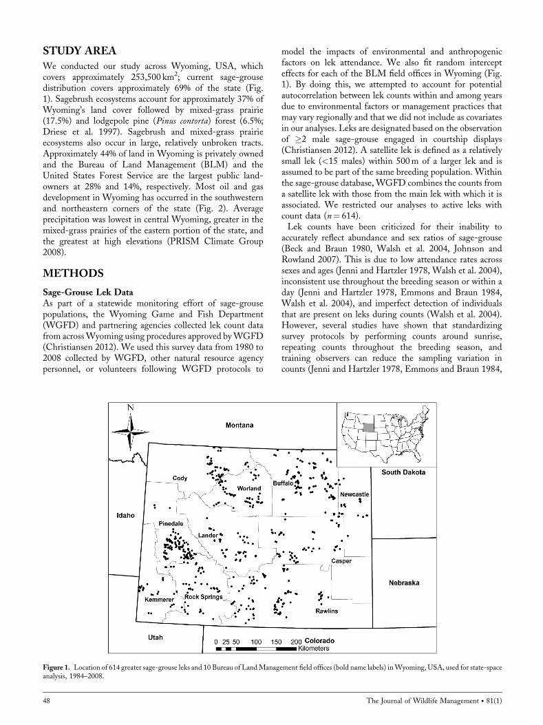
We conducted our study across Wyoming, USA, whichcovers approximately 253,500 km2; current sage-grousedistribution covers approximately 69% of the state (Fig.1). Sagebrush ecosystems account for approximately 37% ofWyoming’s land cover followed by mixed-grass prairie(17.5%) and lodgepole pine (Pinus contorta) forest (6.5%;Driese et al. 1997). Sagebrush and mixed-grass prairieecosystems also occur in large, relatively unbroken tracts.Approximately 44% of land in Wyoming is privately ownedand the Bureau of Land Management (BLM) and theUnited States Forest Service are the largest public land-owners at 28% and 14%, respectively. Most oil and gasdevelopment in Wyoming has occurred in the southwesternand northeastern corners of the state (Fig. 2). Averageprecipitation was lowest in central Wyoming, greater in themixed-grass prairies of the eastern portion of the state, andthe greatest at high elevations (PRISM Climate Group2008).

METHODS

Sage-Grouse Lek DataAs part of a statewide monitoring effort of sage-grousepopulations, the Wyoming Game and Fish Department(WGFD) and partnering agencies collected lek count datafrom acrossWyoming using procedures approved byWGFD(Christiansen 2012). We used this survey data from 1980 to2008 collected by WGFD, other natural resource agencypersonnel, or volunteers following WGFD protocols to

model the impacts of environmental and anthropogenicfactors on lek attendance. We also fit random intercepteffects for each of the BLM field offices in Wyoming (Fig.1). By doing this, we attempted to account for potentialautocorrelation between lek counts within and among yearsdue to environmental factors or management practices thatmay vary regionally and that we did not include as covariatesin our analyses. Leks are designated based on the observationof �2 male sage-grouse engaged in courtship displays(Christiansen 2012). A satellite lek is defined as a relativelysmall lek (<15 males) within 500m of a larger lek and isassumed to be part of the same breeding population. Withinthe sage-grouse database, WGFD combines the counts froma satellite lek with those from the main lek with which it isassociated. We restricted our analyses to active leks withcount data (n¼ 614).Lek counts have been criticized for their inability to

accurately reflect abundance and sex ratios of sage-grouse(Beck and Braun 1980, Walsh et al. 2004, Johnson andRowland 2007). This is due to low attendance rates acrosssexes and ages (Jenni and Hartzler 1978, Walsh et al. 2004),inconsistent use throughout the breeding season or within aday (Jenni and Hartzler 1978, Emmons and Braun 1984,Walsh et al. 2004), and imperfect detection of individualsthat are present on leks during counts (Walsh et al. 2004).However, several studies have shown that standardizingsurvey protocols by performing counts around sunrise,repeating counts throughout the breeding season, andtraining observers can reduce the sampling variation incounts (Jenni and Hartzler 1978, Emmons and Braun 1984,

Figure 1. Location of 614 greater sage-grouse leks and 10 Bureau of LandManagement field offices (bold name labels) inWyoming, USA, used for state-spaceanalysis, 1984–2008.

48 The Journal of Wildlife Management � 81(1)

Walsh et al. 2004, Johnson and Rowland 2007) and provide areasonable index with which to estimate population trends(Blomberg et al. 2013). Leks were sampled by WGFD fromearly March to early May to coincide with the peak of thebreeding season based on latitude, elevation, and weather(Jenni and Hartzler 1978, Emmons and Braun 1984, Walshet al. 2004, Christiansen 2012). We used only counts thatoccurred between 30minutes pre-sunrise to 90minutes post-sunrise, the most active lekking period of the day (Jenni andHartzler 1978), which increases the likelihood that countsrepresent the maximum number of sage-grouse present on agiven day. The WGFD recommends that counts occurbetween 30minutes pre-sunrise to 60minutes post-sunrise.Simulations have shown little difference in estimates or lossof precision in extending counts to 90minutes post-sunrise(Monroe et al. 2016), so we included these counts to increasesample sizes. Because male sage-grouse have higher andmore regular lek attendance than females (Emmons andBraun 1984, Walsh et al. 2004), we used the maximum malecount within a year at a lek. Additionally, we restricted ouranalysis to leks with�2 counts over the study period, becauseour parameter of interest was the change in lek attendanceacross years rather than the counts themselves. Theserestrictions resulted in a data set consisting of 3,382 lek-yearcounts at 614 leks from 1984–2008 (Fig. 1).

Oil and Gas DataWe obtained information on oil and gas well characteristicsand locations from the Wyoming Oil and Gas ConservationCommission (WOGCC; WOGCC 2011) for 1980–2008.

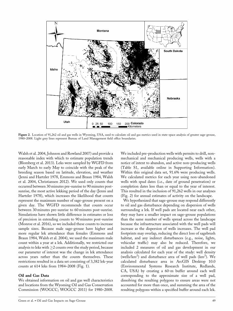
We included pre-production wells with permits to drill, non-mechanical and mechanical producing wells, wells with anotice of intent to abandon, and active non-producing wells(Table S1, available online in Supporting Information).Within this original data set, 91.6% were producing wells.We calculated metrics for each year using non-abandonedwells with spud dates (i.e., date of ground penetration) orcompletion dates less than or equal to the year of interest.This resulted in the inclusion of 91,262 wells in our analyses(Fig. 2) for annual estimates of activity on the landscape.We hypothesized that sage-grouse may respond differently

to oil and gas disturbance depending on dispersion of wellssurrounding a lek. If well pads are located near each other,they may have a smaller impact on sage-grouse populationsthan the same number of wells spread across the landscapebecause the infrastructure associated with the well pads willincrease as the dispersion of wells increases. The well padfootprints may overlap, reducing the direct loss of sagebrushhabitat, and any indirect disturbances (e.g., noise, lights,vehicular traffic) may also be reduced. Therefore, weincluded 2 measures of oil and gas development in ouranalysis calculated for each year of the study: well density(wells/km2) and disturbance area of well pads (km2). Wecalculated disturbance area in ArcGIS Desktop 10.0(Environmental Systems Research Institute, Redlands,CA, USA) by creating a 60-m buffer around each wellcorresponding to the approximate size of a well pad,dissolving the resulting polygons to ensure areas were notaccounted for more than once, and summing the area of theresulting polygons within a specified buffer around each lek.

Figure 2. Location of 91,262 oil and gas wells in Wyoming, USA, used to calculate oil and gas metrics used in state-space analysis of greater sage-grouse,1980–2008. Light grey lines represent Bureau of Land Management field office boundaries.

Green et al. � Oil and Gas Impacts on Sage-Grouse 49

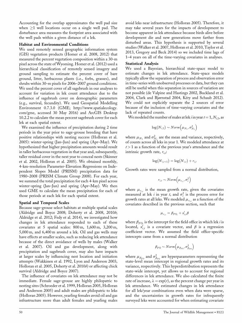
Accounting for the overlap approximates the well pad sizewhen �1 well locations occur on a single well pad. Thedisturbance area measures the footprint area associated withthe well pads within a given distance of a lek.

Habitat and Environmental ConditionsWe used remotely sensed geographic information system(GIS) vegetation products (Homer et al. 2008, 2012) thatmeasured the percent vegetation composition within a 30-mpixel across the state ofWyoming. Homer et al. (2012) used ahierarchical classification of remotely sensed imagery andground sampling to estimate the percent cover of bareground, litter, herbaceous plants (i.e., forbs, grasses), andshrubs within 30-m pixels for 2006–2007 ground conditions.We used the percent cover of all sagebrush in our analyses toaccount for variation in lek count attendance due to theinfluence of sagebrush cover on demographic parameters(e.g., survival, fecundity). We used Geospatial ModellingEnvironment 0.7.3.0 (GME; http://www.spatialecology.com/gme, accessed 30 May 2016) and ArcGIS Desktop10.2.2 to calculate the mean percent sagebrush cover for eachlek at each spatial extent.We examined the influence of precipitation during 2 time

periods in the year prior to sage-grouse breeding that havepositive relationships with nesting success (Holloran et al.2005): winter-spring (Jan–Jun) and spring (Apr–May). Wehypothesized that higher precipitation amounts would resultin taller herbaceous vegetation in that year and, subsequently,taller residual cover in the next year to conceal nests (Skinneret al. 2002, Holloran et al. 2005). We obtained monthly,4-km-resolution Parameter-Elevation Regressions on Inde-pendent Slopes Model (PRISM) precipitation data for1980–2008 (PRISM Climate Group 2008). For each year,we summed the total precipitation for each 4-km pixel acrosswinter-spring (Jan–Jun) and spring (Apr–May). We thenused GME to calculate the mean precipitation for each ofthose periods at each lek for each spatial extent.

Spatial and Temporal ScalesBecause sage-grouse select habitats at multiple spatial scales(Aldridge and Boyce 2008; Doherty et al. 2008, 2010b;Aldridge et al. 2012; Fedy et al. 2014), we investigated howchanges in lek attendance responded to each of thesecovariates at 5 spatial scales: 800m, 1,600m, 3,200m,5,000m, and 6,400m around a lek. Oil and gas wells mayhave effects at smaller scales, such as reducing lek attendancebecause of the direct avoidance of wells by males (Walkeret al. 2007). Oil and gas development, along withprecipitation and sagebrush cover, may also have impactsat larger scales by influencing nest location and initiationattempts (Wakkinen et al. 1992, Lyon and Anderson 2003,Holloran et al. 2005, Doherty et al. 2010b) or affecting chicksurvival (Aldridge and Boyce 2007).The influence of covariates on lek attendance may not be

immediate. Female sage-grouse are highly philopatric tonesting sites (Schroeder et al. 1999, Holloran 2005, Holloranand Anderson 2005) and adult males are philopatric to leks(Holloran 2005). However, yearling females avoid oil and gasinfrastructure more than adult females and yearling males

avoid leks near infrastructure (Holloran 2005). Therefore, itmay take several years for the impacts of development tobecome apparent in lek attendance because birds alive beforedevelopment die and new generations move farther fromdisturbed areas. This hypothesis is supported by severalstudies (Walker et al. 2007, Holloran et al. 2010, Taylor et al.2013, Gregory and Beck 2014) so we included time lags of1–4 years on all of the time-varying covariates in analyses.

Statistical AnalysisWe used a Bayesian, hierarchical state-space model toestimate changes in lek attendance. State-space modelstypically allow the separation of process and observation errorin time-series with unobserved processes or data, but they canstill be useful when this separation in sources of variation arenot possible (de Valpine and Hastings 2002, Buckland et al.2004, Clark and Bjørnstad 2004, K�ery and Schaub 2012).We could not explicitly separate the 2 sources of errorbecause of the inclusion of time-varying covariates and thelack of repeated counts.Wemodeled thenumber ofmales at lek i in year t¼ 1,Ni,1, as

log Ni;1

� � � Norm mN 1; s2

N 1

� �

where mN 1and s2

N 1are the mean and variance, respectively,

of counts across all leks in year 1. We modeled attendance att> 1 as a function of the previous year’s attendance and theintrinsic growth rate, ri,t:

log Ni;tþ1

� � ¼ log Ni;t

� �þ ri;t

Growth rates were sampled from a normal distribution,

ri;t � Norm mri;t ; s2r

� �

where mri;t is the mean growth rate, given the covariatesmeasured at lek i in year t, and s2

r is the process error forgrowth rates at all leks. We modeled mri;t as a function of thecovariates described in the previous section, such that

mri;t ¼ bFOiþ x0i;tb

where bFOiis the intercept for the field office in which lek i is

located, x0i;t is a covariate vector, and b is a regressioncoefficient vector. We assumed the field office-specificintercepts came from a normal distribution

bFO � Norm mbFO; s2

bFO

� �

where mbFOand s2

bFOare hyperparameters representing the

state-level mean intercept in regional growth rates and itsvariance, respectively. This hyperdistribution represents thestate-wide intercept, yet allows us to account for regionaldifferences in lek attendance. We also calculated the finiterate of increase, l¼ exp(r), as the percent change per year inlek attendance. We estimated changes in lek attendancefor all lek/year combinations even when data were sparse,and the uncertainties in growth rates for infrequentlysurveyed leks were accounted for when estimating covariate

50 The Journal of Wildlife Management � 81(1)

relationships. We standardized all covariates so that theyhad a mean of 0 and standard deviation of 1. To model theobservation process, we assumed that the maximum malecounts came from a Poisson distribution,

yi;t � Pois N i;t

� �We took a Bayesian approach to estimate model parameters

using Markov chain Monte Carlo (MCMC) simulationimplemented in JAGS 3.4.0 (Plummer 2003, 2013) using thepackage R2jags in the R statistical computing environment(R Core Team 2013). We used vague prior distributions forall estimated parameters:

sr � Unif 0; 20ð Þ

mbFO� Norm 0; 100ð Þ

sbFO � Unif 0; 20ð Þ

and

b � Norm 0; 100ð ÞWe converted all standard deviations to precision (1/SD2)

for implementation in JAGS.Because of the large number of possible combinations of

covariates and the high correlation between covariates withina group of covariates (i.e., oil and gas, sagebrush cover,precipitation), we used a sequential approach to modelbuilding. We fit all univariable models and chose the bestpredictive model (see next paragraph) from each covariategroup to include in the next step of model building. We thenfit models for all additive and 2-way interactive combinationsof the top covariates from each covariate group. We alsoincluded a null model to represent the overall lek trend acrosstime and a quadratic term for the top oil and gas covariate inour final model set to test for thresholds, where lekattendance may not be affected by low levels of development(Doherty et al. 2010a). We obtained 20,000 MCMCsamples and used a burn-in period of 10,000 iterations formodels in the final model set from which we made inferencesregarding the factors influencing sage-grouse lek attendance.We used 10-fold cross-validation to measure the perfor-

mance of the models in our model sets (Hooten and Hobbs2015). Cross-validation consists of grouping the data into Kapproximately even groups, fitting a model to the dataexcluding that in group k, y�k, and comparing predictions forthe left out data, yk. We repeated the process for each groupof data and calculated a metric for each iteration and summedacross all iterations to produce a cross-validation score for theentire data set. We calculated our cross-validation score(CVS) as

CVS ¼ �2XK

k¼1log

XT

t¼1½ykjy�k; u

tð Þ�T

0@

1A

where ½ykjy�k; utð Þ� is the likelihood of yk, given y�k and u(t),

the tth MCMC sample (out of T total MCMC samples) of

the model parameters. Unlike more widely used modelselection criteria (e.g., Akaike’s Information Criterion),there is no general rule of thumb regarding the amount ofevidence provided by cross-validation scores within a modelset (Hooten and Hobbs 2015); it is merely a measure of thepredictive ability of a model. We considered the model withthe smallest CVS to be the best model.We used 3 chains and computed the Gelman-Rubin

convergence statistic (R̂), which was <1.1 for all modelparameters (Gelman and Rubin 1992, Brooks and Gelman1998) to determine when the algorithms converged. Weassessed the fit of the models using a Bayesian P-value basedon the mean squared error (K�ery and Schaub 2012),

P ¼XT

t¼1MSEt

T

where

MSEt

1; if S

�y �by� �2k

> Sy �by� �2

k

0; if S

�y �by� �2k

� Sy �by� �2

k

8>>><>>>:

and y is the observed data, by is the predicted data,�y is

simulated data based on MCMC samples at iteration T, andk is the sample size. A P-value>0.05 suggests sufficient fit ofthe model to the data (Hooten and Hobbs 2015).

RESULTS

As expected, most oil and gas covariates were correlatedacross space and time. Seventy-five percent of the 780combinations of oil and gas metrics, including spatial scalesand lag, had Pearson’s correlation coefficients r> 0.70, witha minimum of r¼ 0.56. Percent sagebrush at the 3 scales wascorrelated, with all r� 0.940. Winter-spring and springprecipitation were correlated across scales for a given lag(all r> 0.65) but were uncorrelated across lags (range:0.05–0.45).Lek attendance decreased by 2.5% (l¼ 0.975, 95% credible

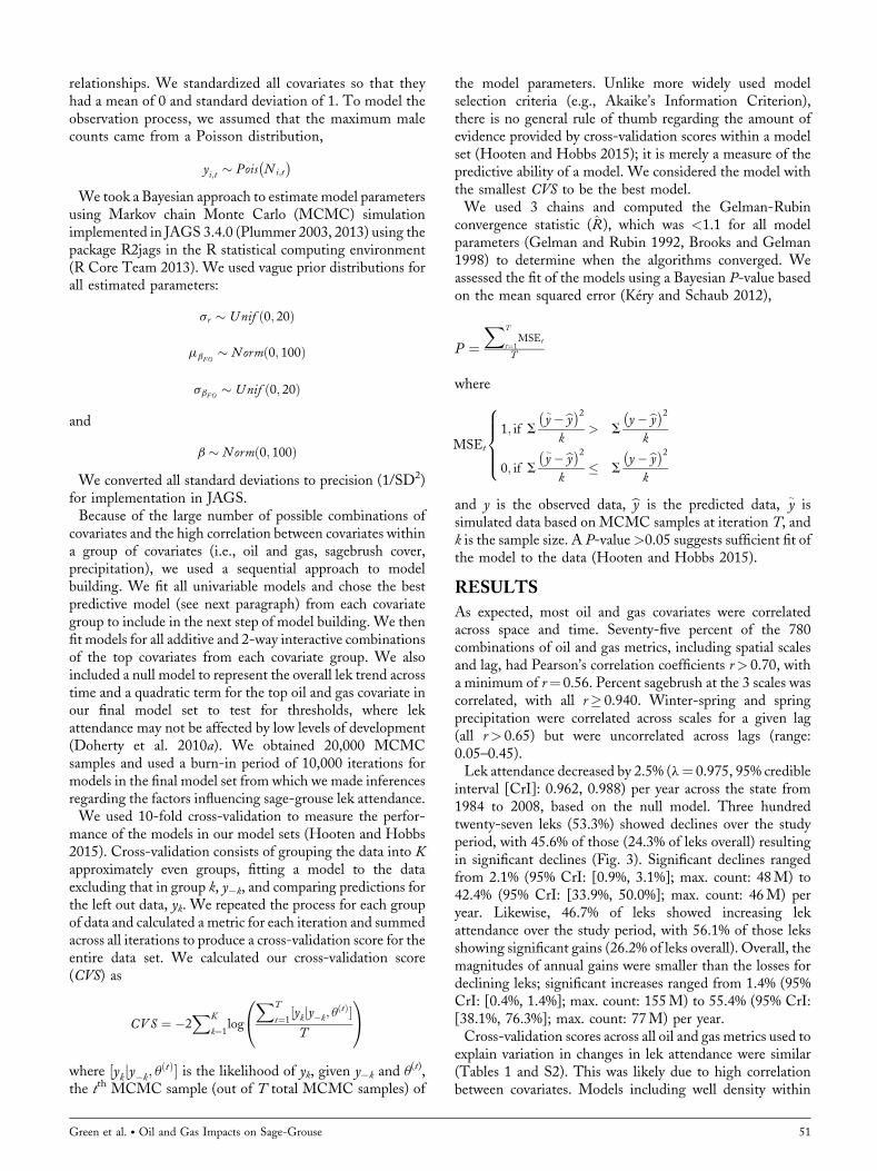
interval [CrI]: 0.962, 0.988) per year across the state from1984 to 2008, based on the null model. Three hundredtwenty-seven leks (53.3%) showed declines over the studyperiod, with 45.6% of those (24.3% of leks overall) resultingin significant declines (Fig. 3). Significant declines rangedfrom 2.1% (95% CrI: [0.9%, 3.1%]; max. count: 48M) to42.4% (95% CrI: [33.9%, 50.0%]; max. count: 46M) peryear. Likewise, 46.7% of leks showed increasing lekattendance over the study period, with 56.1% of those leksshowing significant gains (26.2% of leks overall). Overall, themagnitudes of annual gains were smaller than the losses fordeclining leks; significant increases ranged from 1.4% (95%CrI: [0.4%, 1.4%]; max. count: 155M) to 55.4% (95% CrI:[38.1%, 76.3%]; max. count: 77M) per year.Cross-validation scores across all oil and gas metrics used to

explain variation in changes in lek attendance were similar(Tables 1 and S2). This was likely due to high correlationbetween covariates. Models including well density within

Green et al. � Oil and Gas Impacts on Sage-Grouse 51

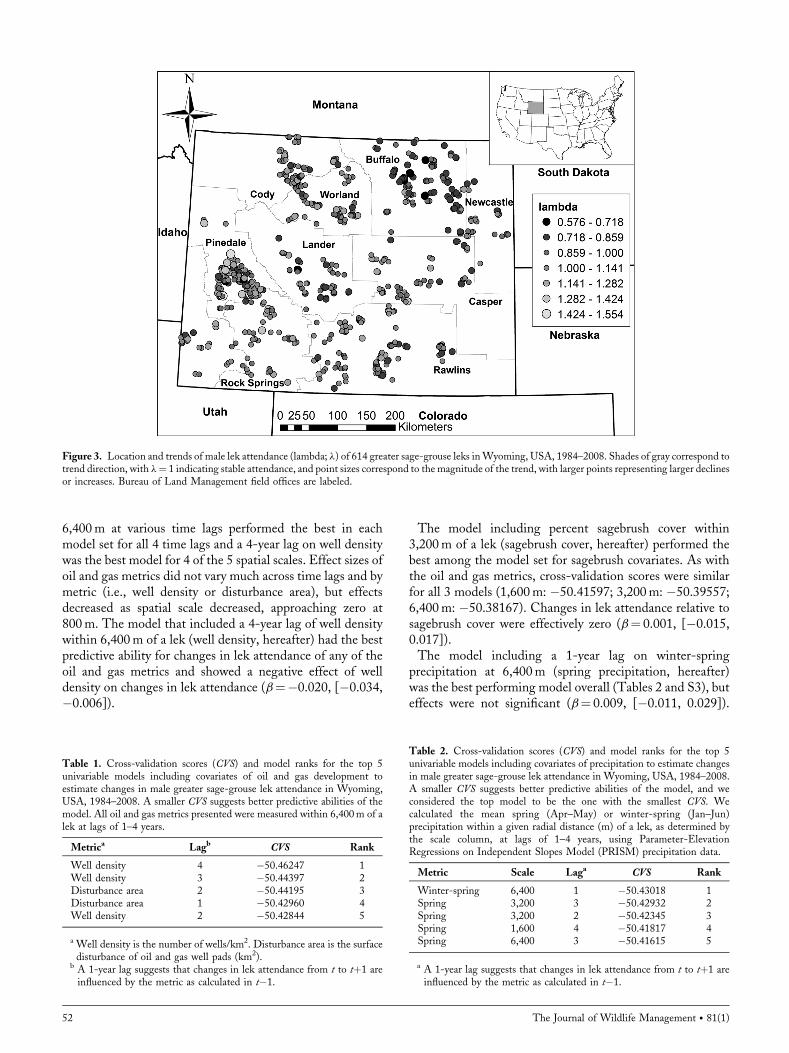
6,400m at various time lags performed the best in eachmodel set for all 4 time lags and a 4-year lag on well densitywas the best model for 4 of the 5 spatial scales. Effect sizes ofoil and gas metrics did not vary much across time lags and bymetric (i.e., well density or disturbance area), but effectsdecreased as spatial scale decreased, approaching zero at800m. The model that included a 4-year lag of well densitywithin 6,400m of a lek (well density, hereafter) had the bestpredictive ability for changes in lek attendance of any of theoil and gas metrics and showed a negative effect of welldensity on changes in lek attendance (b¼�0.020, [�0.034,�0.006]).

The model including percent sagebrush cover within3,200m of a lek (sagebrush cover, hereafter) performed thebest among the model set for sagebrush covariates. As withthe oil and gas metrics, cross-validation scores were similarfor all 3 models (1,600m: �50.41597; 3,200m: �50.39557;6,400m: �50.38167). Changes in lek attendance relative tosagebrush cover were effectively zero (b¼ 0.001, [�0.015,0.017]).The model including a 1-year lag on winter-spring

precipitation at 6,400m (spring precipitation, hereafter)was the best performing model overall (Tables 2 and S3), buteffects were not significant (b¼ 0.009, [�0.011, 0.029]).

Figure 3. Location and trends of male lek attendance (lambda; l) of 614 greater sage-grouse leks inWyoming, USA, 1984–2008. Shades of gray correspond totrend direction, with l¼ 1 indicating stable attendance, and point sizes correspond to the magnitude of the trend, with larger points representing larger declinesor increases. Bureau of Land Management field offices are labeled.

Table 1. Cross-validation scores (CVS) and model ranks for the top 5univariable models including covariates of oil and gas development toestimate changes in male greater sage-grouse lek attendance in Wyoming,USA, 1984–2008. A smaller CVS suggests better predictive abilities of themodel. All oil and gas metrics presented were measured within 6,400m of alek at lags of 1–4 years.

Metrica Lagb CVS Rank

Well density 4 �50.46247 1Well density 3 �50.44397 2Disturbance area 2 �50.44195 3Disturbance area 1 �50.42960 4Well density 2 �50.42844 5

a Well density is the number of wells/km2. Disturbance area is the surfacedisturbance of oil and gas well pads (km2).

b A 1-year lag suggests that changes in lek attendance from t to tþ1 areinfluenced by the metric as calculated in t�1.

Table 2. Cross-validation scores (CVS) and model ranks for the top 5univariable models including covariates of precipitation to estimate changesin male greater sage-grouse lek attendance in Wyoming, USA, 1984–2008.A smaller CVS suggests better predictive abilities of the model, and weconsidered the top model to be the one with the smallest CVS. Wecalculated the mean spring (Apr–May) or winter-spring (Jan–Jun)precipitation within a given radial distance (m) of a lek, as determined bythe scale column, at lags of 1–4 years, using Parameter-ElevationRegressions on Independent Slopes Model (PRISM) precipitation data.

Metric Scale Laga CVS Rank

Winter-spring 6,400 1 �50.43018 1Spring 3,200 3 �50.42932 2Spring 3,200 2 �50.42345 3Spring 1,600 4 �50.41817 4Spring 6,400 3 �50.41615 5

a A 1-year lag suggests that changes in lek attendance from t to tþ1 areinfluenced by the metric as calculated in t�1.

52 The Journal of Wildlife Management � 81(1)

There were no obvious patterns in models includingprecipitation covariates across time lags or spatial scales.Models including well density performed the best within

our final model set, with 10 of the top 11 models includingwell density. The top model included well density and aninteractive term between sagebrush cover and winter-springprecipitation (Table 3). However, CVSs were the same to 2decimal places for the 2 best models.We used the second bestmodel (well density only) to make inferences because of thesmall differences in CVSs and because the sagebrush coverand precipitation main effects and their interaction weresmall and their 95% credible intervals included zero. Themodel that included a quadratic term on well density did notperform well and the null model performed the second worstin our final model set (Table 3). The Bayesian P-value for thebest overall model (Bayesian P¼ 0.46) suggested an adequatefit of the model to the data.Lek attendance in the average field office, given the average

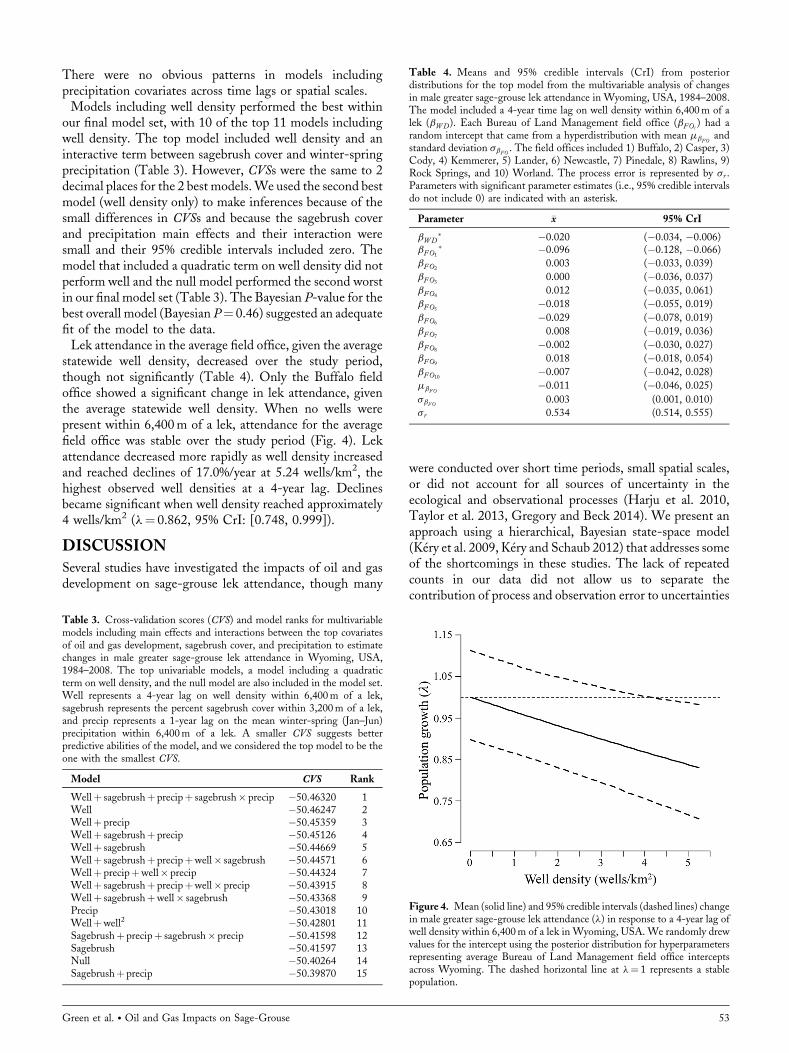
statewide well density, decreased over the study period,though not significantly (Table 4). Only the Buffalo fieldoffice showed a significant change in lek attendance, giventhe average statewide well density. When no wells werepresent within 6,400m of a lek, attendance for the averagefield office was stable over the study period (Fig. 4). Lekattendance decreased more rapidly as well density increasedand reached declines of 17.0%/year at 5.24 wells/km2, thehighest observed well densities at a 4-year lag. Declinesbecame significant when well density reached approximately4 wells/km2 (l¼ 0.862, 95% CrI: [0.748, 0.999]).

DISCUSSION

Several studies have investigated the impacts of oil and gasdevelopment on sage-grouse lek attendance, though many

were conducted over short time periods, small spatial scales,or did not account for all sources of uncertainty in theecological and observational processes (Harju et al. 2010,Taylor et al. 2013, Gregory and Beck 2014). We present anapproach using a hierarchical, Bayesian state-space model(K�ery et al. 2009, K�ery and Schaub 2012) that addresses someof the shortcomings in these studies. The lack of repeatedcounts in our data did not allow us to separate thecontribution of process and observation error to uncertainties

Table 3. Cross-validation scores (CVS) and model ranks for multivariablemodels including main effects and interactions between the top covariatesof oil and gas development, sagebrush cover, and precipitation to estimatechanges in male greater sage-grouse lek attendance in Wyoming, USA,1984–2008. The top univariable models, a model including a quadraticterm on well density, and the null model are also included in the model set.Well represents a 4-year lag on well density within 6,400m of a lek,sagebrush represents the percent sagebrush cover within 3,200m of a lek,and precip represents a 1-year lag on the mean winter-spring (Jan–Jun)precipitation within 6,400m of a lek. A smaller CVS suggests betterpredictive abilities of the model, and we considered the top model to be theone with the smallest CVS.

Model CVS Rank

Wellþ sagebrushþ precipþ sagebrush� precip �50.46320 1Well �50.46247 2Wellþ precip �50.45359 3Wellþ sagebrushþ precip �50.45126 4Wellþ sagebrush �50.44669 5Wellþ sagebrushþ precipþwell� sagebrush �50.44571 6Wellþ precipþwell� precip �50.44324 7Wellþ sagebrushþ precipþwell� precip �50.43915 8Wellþ sagebrushþwell� sagebrush �50.43368 9Precip �50.43018 10Wellþwell2 �50.42801 11Sagebrushþ precipþ sagebrush� precip �50.41598 12Sagebrush �50.41597 13Null �50.40264 14Sagebrushþ precip �50.39870 15

Table 4. Means and 95% credible intervals (CrI) from posteriordistributions for the top model from the multivariable analysis of changesin male greater sage-grouse lek attendance in Wyoming, USA, 1984–2008.The model included a 4-year time lag on well density within 6,400m of alek (bWD). Each Bureau of Land Management field office (bFOi

) had arandom intercept that came from a hyperdistribution with mean mbFO

andstandard deviation sbFO . The field offices included 1) Buffalo, 2) Casper, 3)Cody, 4) Kemmerer, 5) Lander, 6) Newcastle, 7) Pinedale, 8) Rawlins, 9)Rock Springs, and 10) Worland. The process error is represented by sr .Parameters with significant parameter estimates (i.e., 95% credible intervalsdo not include 0) are indicated with an asterisk.

Parameter �x 95% CrI

bWD �0.020 (�0.034, �0.006)

bFO1

�0.096 (�0.128, �0.066)

bFO20.003 (�0.033, 0.039)

bFO30.000 (�0.036, 0.037)

bFO40.012 (�0.035, 0.061)

bFO5�0.018 (�0.055, 0.019)

bFO6�0.029 (�0.078, 0.019)

bFO70.008 (�0.019, 0.036)

bFO8�0.002 (�0.030, 0.027)

bFO90.018 (�0.018, 0.054)

bFO10�0.007 (�0.042, 0.028)

mbFO�0.011 (�0.046, 0.025)

sbFO 0.003 (0.001, 0.010)

sr 0.534 (0.514, 0.555)

Figure 4. Mean (solid line) and 95% credible intervals (dashed lines) changein male greater sage-grouse lek attendance (l) in response to a 4-year lag ofwell density within 6,400m of a lek in Wyoming, USA. We randomly drewvalues for the intercept using the posterior distribution for hyperparametersrepresenting average Bureau of Land Management field office interceptsacross Wyoming. The dashed horizontal line at l¼ 1 represents a stablepopulation.

Green et al. � Oil and Gas Impacts on Sage-Grouse 53

in the response of lek attendance to covariates. However, thisapproach allowed us to make inference to a larger number ofleks and over longer time periods by borrowing informationfrom well-sampled leks to predict counts at poorly sampledleks. Uncertainties in the relationships between attendance atpoorly sampled leks and oil and gas disturbance areaccounted for in coefficient estimates, and, despite theseuncertainties, we were still able to confirm the generalfindings of previous studies.We estimated statewide annual declines in lek attendance

of 2.5% based on our null model, which is similar to trendsestimated in other studies for various Wyoming sage-grousepopulations (Walker et al. 2007, Garton et al. 2011, Gregoryand Beck 2014). However, as with other studies, we saw alarge range of growth rates across our study area (Fig. 3) anddeclines were associated with higher well densities. Oil andgas development correlates well with sage-grouse populationdeclines from 1984 to 2008 inWyoming, which is supportedby other findings (Doherty et al. 2010b, Harju et al. 2010,Hess and Beck 2012, Taylor et al. 2013, Gregory and Beck2014). As with other studies, we also found support for 4-year lag effects of oil and gas development on lek attendance(Walker et al. 2007, Doherty et al. 2010a, Harju et al. 2010,Gregory and Beck 2014). This result suggests thatdevelopment likely affects recruitment into the breedingpopulation rather than avoidance of wells by adult males oradult survival. Adult sage-grouse are highly philopatric to leksites (Dalke et al. 1963, Wallestad and Schladweiler 1974,Emmons and Braun 1984, Dunn and Braun 1985, Connellyet al. 2011a), and males typically recruit to the breedingpopulation in 2–3 years. We would expect a delayed responsein lek attendance if development affects recruitment, eitherby reducing fecundity or avoidance of disturbance by nestingfemales, as adult males die and are not replaced by youngmales.On average, lek attendance was stable when no oil and gas

development was present within 6,400m (Fig. 4). However,attendance declined as development increased. Declines didnot become significant until well density reached approxi-mately 4wells/km2; at this well density, we predict meandeclines of nearly 14%/year (l¼ 0.862, 95% CrI: [0.748,0.999]). In 2008, Wyoming implemented measures toprotect core areas of the sage-grouse population under theSage-Grouse Executive Order (State of Wyoming 2008,2015). The intent of this executive order was to maintainhabitat for a large portion of Wyoming’s sage-grousepopulation through fire suppression, habitat management,and limiting oil and gas development. The density of activewells near a lek within a core area is limited to 0.39well pads/km2 (State of Wyoming 2015), which may contain up to64wells/pad. The linear relationships we found between welldensity and lek attendance may not hold at such highdensities, but even 1well/pad at this pad density wouldcorrespond to a decline of approximately 1.4%/year(l¼ 0.986, 95% CrI: [0.885, 1.100]) within core areas,based on our results (Fig. 4). These predicted declines are notsignificant because of the uncertainty associated with lekcounts and sparse data but suggest that declines in sage-

grouse populations may continue within core areas at thesedevelopment levels.Though several studies have examined the impacts of oil

and gas development on sage-grouse lek attendance, weprovide the first comparison of 2 measures of disturbance dueto development. Other studies have typically used well orwell pad density at various spatial scales and time lags as ameasure of oil and gas development (Doherty et al. 2010a,Harju et al. 2010, Hess and Beck 2012, Taylor et al. 2013,Gregory and Beck 2014). However, the distribution of wellsaround a lek may play an important role in the magnitude ofthe impacts (Walker et al. 2007), so we fit models includingdisturbance area to account for these differences. If wells arelocated close to other wells, disturbance due to light andnoise will be concentrated in a smaller area, leaving a largerproportion of the landscape undisturbed. Additionally, fewerroads and pipelines may be necessary, resulting in reducedinfrastructure and less habitat fragmentation and disturbancefrom vehicular traffic. We were unable to find differencesbetween the models that included well density and those thatincluded disturbance area because of high correlationbetween these covariates, suggesting that a simple measureof well density may be suitable to capture correlative effects ofenergy development on sage-grouse population trends acrossbroad geographic extents. This does not dismiss that morelocal impacts on survival may be occurring in response to howdevelopment takes place (Holloran et al. 2005, Aldridge andBoyce 2007).There was only one BLM field office that showed

significant declines over the study period (Buffalo; TableS4). However, the largest mean growth for any field officewas only 2.1%/year (l¼ 1.021, [0.990, 1.052]), suggestingthat future development may result in declines in thesecurrently stable regions. We acknowledge that BLM fieldoffices may be too large and arbitrary to represent naturalgroupings of leks that respond to local habitat and weatherconditions, but all models including random intercepts forfield office performed better than the best fixed-interceptmodel we fit in preliminary analyses. This suggests that someautocorrelation in changes in lek attendance occurs at thisscale and it may provide a useful way to group leks to accountfor this correlation and improve the precision of estimates.We found little evidence that the amount of sagebrush

surrounding a lek influenced changes in lek attendance.However, numerous studies have described the importanceof sagebrush to sage-grouse throughout their life cycle(Remington and Braun 1985, Gregg et al. 1994, Holloranet al. 2005, Doherty et al. 2010b, Fedy et al. 2014).Therefore, we think that the effects of sagebrush in ourmodels were small and imprecise (coefficient of variation, s/m¼ 7.76) because we were only able to obtain estimates ofsagebrush cover from 2006 to 2007. Changes in sagebrushcover are negatively correlated with changes in well densitybecause oil and gas development often occurs in areas of highsagebrush cover (Knick et al. 2003, Connelly et al. 2011b,Finn and Knick 2011) and removes sagebrush habitat.Though time-varying estimates of sagebrush cover wouldbetter represent changes in available habitat throughout the

54 The Journal of Wildlife Management � 81(1)

study period, we expected the single estimate to representsagebrush abundance. In addition, having an estimate fromnear the end of our study period allows us to evaluate thecumulative impacts of sagebrush loss at leks and itcorresponds to the years with the highest data coverage.More frequent measures of sagebrush cover for southwesternWyoming are being estimated (C. G. Homer, United StatesGeological Survey, unpublished data), and future studiesshould investigate the impacts of changes in sagebrush coverover time on sage-grouse population trends (lek attendance).Precipitation can have a positive influence on nesting

success, clutch size, and chick and juvenile survival (Holloranet al. 2005, Blomberg et al. 2014a,b), potentially resulting inimpacts on male lek attendance as males enter the breedingpopulation. We found little evidence for the effect ofprecipitation on lek attendance and responses to lags werenot differentiated. The lack of evidence for strong impacts ofprecipitation is possibly due to the scale of the PRISM dataused in our analyses (i.e., 4-km). This extent may be toocoarse spatially and temporally to capture the mechanismsinfluencing sage-grouse recruitment or the error associatedwith estimation of these metrics may be too large,overwhelming any potential effects. However, other studieson sage-grouse in the Great Basin used similar measures andfound positive responses of recruitment and populationgrowth to increasing precipitation (Blomberg et al. 2012,Coates et al. 2015). The Great Basin has lower annualprecipitation and drier and warmer soils than Wyoming(Coates et al. 2015), and its sage-grouse populations may bemore sensitive to precipitation. Finally, the timing ofprecipitation may play an important role in how sage-grousepopulations respond. We included time periods shown toaffect recruitment in Wyoming (Holloran et al. 2005).However, precipitation during other times may influenceother demographic parameters, such as adult survival, towhich populations may be more sensitive. Future studiesshould investigate the importance of precipitation timing onvarious demographic vital rates and population growth.We acknowledge that lek counts are not an ideal direct

measure of sage-grouse populations. Attendance rates ofsage-grouse vary throughout the day, breeding season, andacross sexes and age classes (Jenni and Hartzler 1978,Emmons and Braun 1984, Walsh et al. 2004, Johnson andRowland 2007). However, survey protocols are standardizedwithin Wyoming to ensure that maximum male countsprovide a reasonable index to abundance (Fedy and Aldridge2011, Christiansen 2012, Blomberg et al. 2013). Theassumption that detection rates of sage-grouse are constantacross surveys and observers poses an additional problem(Walsh et al. 2004). Even if the number of males present at alek is constant across surveys, counts will provide a biasedindex of abundance if detection probabilities are not constant(Anderson 2001). Standardization of protocols and trainingof observers likely reduces the variation in detectionprobabilities so that changes in lek counts more accuratelyreflect changes in abundance rather than detection (Walshet al. 2004). Additionally, our model included an error termto account for some of the variation in counts due to process

error and assumed counts were a random variable, accountingfor observation error. Because we could not assume closure ofthe lek-attending sage-grouse population between surveys,we were able to use only 1 count from each lek in a given year.Having additional counts, possibly from a second observercounting at the same time, could provide replication toestimate detection probabilities (Nichols et al. 2000, Forceyet al. 2006) and tease apart variation due to process andobservation error. However, this requires financial andpersonnel resources, and tradeoffs between replication andthe number of leks sampled should be assessed based on theinformation desired by management agencies (Fedy andAldridge 2011).

MANAGEMENT IMPLICATIONS

Our findings contribute to the growing number of studiessuggesting oil and gas development has negative impacts onsage-grouse populations and suggest that current regulationsmay only be sufficient for limiting population declines butnot for reversing these trends. Additionally, areas notprotected under the executive order are not subject to core-area regulations and may experience larger increases in oiland gas development and, therefore, larger declines in sage-grouse populations.

ACKNOWLEDGMENTS

Any use of trade, firm, or product names is for descriptivepurposes only and does not imply endorsement by the U.S.Government. The authors do not have any conflicts ofinterest to report. We thank WGFD for use of lek surveydata and all personnel that performed lek counts. A largenumber of people provided input throughout the analysis,particularly A. P. Monroe, D. R. Edmunds, J. A. Heinrichs,and D. J. Manier. M. B. Hooten and N. T. Hobbs provideduseful discussion about the model structure and modelselection. We thank P. S. Coates, S. L. Garman, and 2anonymous reviewers for valuable feedback on previousversions of the manuscript. United States Geological SurveyFort Collins Science Center and the Wyoming LandscapeConservation Initiative provided funding for this research.

LITERATURE CITEDAldridge, C. L., and M. S. Boyce. 2007. Linking occurrence and fitness topersistence: a habitat-based approach for greater sage-grouse. EcologicalApplications 17:508–526.

Aldridge, C. L., and M. S. Boyce. 2008. Accounting for fitness: combiningsurvival and selection when assessing wildlife-habitat relationships. IsraelJournal of Ecology and Evolution 54:389–419.

Aldridge, C. L., D. J. Saher, T. M. Childers, K. E. Stahlnecker, and Z. H.Bowen. 2012. Crucial nesting habitat for Gunnison sage-grouse: aspatially explicit hierarchical approach. Journal of Wildlife Management76:391–406.

Anderson, D. R. 2001. The need to get the basics right in wildlife fieldstudies. Wildlife Society Bulletin 29:1294–1297.

Barnett, J. K., and J. A. Crawford. 1994. Pre-laying nutrition of sage grousehens in Oregon. Journal of Range Management 47:114–118.

Bayne, E. M., L. Habib, and S. Boutin. 2008. Impacts of chronicanthropogenic noise from energy-sector activity on abundance ofsongbirds in the boreal forest. Conservation Biology 22:1186–1193.

Beck, T. D. I., and C. E. Braun. 1980. The strutting ground count: variation,traditionalism, management needs. Proceedings of the Western Associa-tion of Fish and Wildlife Agencies 60:558–566.

Green et al. � Oil and Gas Impacts on Sage-Grouse 55

Blomberg, E. J., D. Gibson, M. T. Atamian, and J. S. Sedinger. 2014a.Individual and environmental effects on egg allocations of female greatersage-grouse. Auk 131:507–523.

Blomberg, E. J., J. S. Sedinger, M. T. Atamian, and D. V. Nonne. 2012.Characteristics of climate and landscape disturbance influence thedynamics of greater sage-grouse populations. Ecosphere 3:55. http://dx.doi.org/10.1890/E S11-00304.1

Blomberg, E. J., J. S. Sedinger, D. Gibson, P. S. Coates, andM. L. Casazza.2014b. Carryover effects and climatic conditions influence the postfledgingsurvival of greater sage-grouse. Ecology and Evolution 4:4488–4499.

Blomberg, E. J., J. S. Sedinger, D. V. Nonne, and M. T. Atamian. 2013.Annual male lek attendance influences count-based population indices ofgreater sage-grouse. Journal of Wildlife Management 77:1583–1592.

Brooks, S. P., and A. Gelman. 1998. General methods for monitoringconvergence of iterative simulations. Journal of Computational andGraphical Statistics 7:434–455.

Buckland, S. T., K. B. Newman, L. Thomas, and N. B. Koesters. 2004.State-space models for the dynamics of wild animal populations.Ecological Modelling 171:157–175.

Bunting, S. C., J. L. Kingery, and M. A. Schroeder. 2003. Assessing therestoration potential of altered rangeland ecosystems in the InteriorColumbia Basin. Ecological Restoration 21:77–86.

Carpenter, J. E., C. L. Aldridge, andM. S. Boyce. 2010. Sage-grouse habitatselection during winter in Alberta. Journal of Wildlife Management74:1806–1814.

Christiansen, T. J. 2012. Chapter 12: sage-grouse (Centrocercus urophasia-nus). Pages 12-1–12-55 in S. A. Tessmann and J. R. Bohne, editors.Handbook of biological techniques: third edition. Wyoming Game andFish Department, Cheyenne, USA.

Clark, J. S., and O. N. Bjørnstad. 2004. Population time series: processvariability, observation errors, missing values, lags, and hidden states.Ecology 85:3140–3150.

Coates, P. S., M. A. Ricca, B. G. Prochazka, K. E. Doherty, M. L. Brooks,and M. L. Casazza. 2015. Long-term effects of wildfire on greater sage-grouse—integrating population and ecosystem concepts for managementin the Great Basin. U.S. Geological Survey Open-File Report 2015-1165,Reston, Virginia, USA.

Connelly, J. W., C. A. Hagen, and M. A. Schroeder. 2011a. Characteristicsand dynamics of greater sage-grouse populations. Pages 53–68 in S. T.Knick and J. W. Connelly, editors. Greater sage-grouse: ecology andconservation of a landscape species and its habitats. Studies in AvianBiology, volume 38. University of California Press, Berkeley, USA.

Connelly, J. W., S. T. Knick, M. A. Schroeder, and S. J. Stiver. 2004.Conservation assessment of greater sage-grouse and sagebrush. WesternAssociation of Fish and Wildlife Agencies, Cheyenne, Wyoming, USA.

Connelly, J. W., E. T. Rinkes, and C. E. Braun. 2011b. Characteristics ofgreater sage-grouse habitats: a landscape species at micro and macro scales.Pages 69–83 in S. T. Knick and J. W. Connelly, editors. Greater sage-grouse: ecology and conservation of a landscape species and its habitats.Studies in Avian Biology, volume 38. University of California Press,Berkeley, USA.

Connelly, J. W., M. A. Schroeder, A. R. Sands, and C. E. Braun. 2000.Guidelines to manage sage grouse populations and their habitats. WildlifeSociety Bulletin 28:967–985.

Connelly, J. W., W. L. Waddinen, A. D. Apa, and K. P. Reese. 1991. Sagegrouse use of nest sites in southeastern Idaho. Journal of WildlifeManagement 55:521–524.

Dalke, P. D., D. B. Pyrah, D. C. Stanton, J. E. Crawford, and E. F.Schlatterer. 1963. Ecology, productivity, and management of sage grousein Idaho. Journal of Wildlife Management 27:810–841.

de Valpine, P., and A. Hastings. 2002. Fitting population modelsincorporating process noise and observation error. EcologicalMonographs72:57–76.

Doherty, K. E., D. E. Naugle, and J. S. Evans. 2010a. A currency foroffsetting energy development impacts: horse-trading sage-grouse on theopen market. PLoS ONE 5:e10339.

Doherty, K. E., D. E. Naugle, and B. L.Walker. 2010b. Greater sage-grousenesting habitat: the importance of managing at multiple scales. Journal ofWildlife Management 74:1544–1553.

Doherty, K. E., D. E. Naugle, B. L. Walker, and J. M. Graham. 2008.Greater sage-grouse winter habitat selection and energy development.Journal of Wildlife Management 72:187–195.

Driese, K. L., W. A. Reiners, E. H. Merrill, and K. G. Gerow. 1997.A digital land cover map ofWyoming, USA: a tool for vegetation analysis.Journal of Vegetation Science 8:133–146.

Dunn, P. O., and C. E. Braun. 1985. Natal dispersal and lek fidelity of sagegrouse. Auk 102:621–627.

Dyer, S. J., J. P. O’Neill, S. M. Wasel, and S. Boutin. 2002. Quantifyingbarrier effects of roads and seismic lines onmovements of female woodlandcaribou in northeastern Alberta. Canadian Journal of Zoology80:839–845.

Emmons, S. R., and C. E. Braun. 1984. Lek attendance of male sage grouse.Journal of Wildlife Management 48:1023–1028.

Fedy, B. C., and C. L. Aldridge. 2011. Long-term monitoring of sage-grouse populations: the importance of within-year repeated counts and theinfluence of scale. Journal of Wildlife Management 75:1022–1033.

Fedy, B. C., K. E. Doherty, C. L. Aldridge, M. O’Donnell, J. L. Beck, B.Bedrosian, D. Gummer, M. J. Holloran, G. D. Johnson, N. W. Kaczor,C. P. Kiriol, C. A. Mandich, D. Marshall, G. McKee, C. Olson, A. C.Pratt, C. C. Swanson, and B. L. Walker. 2014. Habitat prioritizationacross large landscapes, multiple seasons, and novel areas: an example usinggreater sage-grouse in Wyoming. Wildlife Monographs 190:1–39.

Finn, S. P., and S. T.Knick. 2011.Changes to theWyomingBasins landscapefromoil and natural gas development. Pages 46–68 in S.E.Hanser,M.Leu,S. T. Knick, and C. L. Aldridge, editors. Sagebrush ecosystem conservationandmanagement: ecoregional assessment tools andmodels for theWyomingBasins. Allen Press, Lawrence, Kansas, USA.

Forcey, G. M., J. T. Anderson, F. K. Ammer, and R. C. Whitmore. 2006.Comparison of two double-observer point-count approaches for estimat-ing breeding bird abundance. Journal of Wildlife Management70:1674–1681.

Francis, C. D., N. J. Kleist, C. P. Ortega, and A. Cruz. 2012. Noise pollutionalters ecological services: enhanced pollination and disrupted seeddispersal. Proceedings of the Royal Society B: Biology 279:2727–2735.

Francis, C. D., C. P. Ortega, and A. Cruz. 2011. Different behaviouralresponses to anthropogenic noise by two closely related passerine birds.Biology Letters 7:850–852.

Garton, E. O., J. W. Connelly, J. S. Horne, C. A. Hagen, A. Moser, andM. A. Schroeder. 2011. Greater sage-grouse population dynamics andprobability of persistence. Pages 293–381 in S. T. Knick and J. W.Connelly, editors. Greater sage-grouse: ecology and conservation of alandscape species and its habitats. Studies in Avian Biology, volume 38.University of California Press, Berkeley, USA.

Gelman, A., and D. B. Rubin. 1992. Inference from iterative simulationusing multiple sequences. Statistical Science 7:457–472.

Gilbert, M. M., and A. D. Chalfoun. 2011. Energy development affectspopulations of sagebrush songbirds in Wyoming. Journal of WildlifeManagement 75:816–824.

Gregg, M. A., J. A. Crawford, M. S. Drut, and A. K. DeLong. 1994.Vegetational cover and predation of sage grouse nests in Oregon. Journalof Wildlife Management 58:162–166.

Gregory, A. J., and J. L. Beck. 2014. Spatial heterogeneity in response ofmale greater sage-grouse lek attendance to energy development. PLoSONE 9:e97132.

Griffin, D. 2002. Prehistoric human impacts on fire regimes and vegetationin the northern Intermountain West. Pages 77–100 in T. R. Vale, editor.Fire, native peoples, and the natural landscape. Island Press, Washington,D.C., USA.

Harju, S. M., M. R. Dzialak, R. C. Taylor, L. D. Hayden-Wing, and J. B.Winstead. 2010. Thresholds and time lags in effects of energydevelopment on greater sage-grouse. Journal of Wildlife Management74:437–448.

Hess, J. E., and J. L. Beck. 2012. Disturbance factors influencing greatersage-grouse lek abandonment in north-central Wyoming. Journal ofWildlife Management 76:1625–1634.

Holloran, M. J. 2005. Greater sage-grouse (Centrocercus urophasianus)population response to natural gas field development in westernWyoming. Dissertation, University of Wyoming, Laramie, USA.

Holloran, M. J, and S. H. Anderson. 2005. Spatial distribution of greatersage-grouse nests in relatively contiguous sagebrush habitats. Condor107:742–752.

Holloran,M. J., B. J. Heath, A. G. Lyon, S. J. Slater, J. L. Kuipers, and S. H.Anderson. 2005. Greater sage-grouse nesting habitat selection and successin Wyoming. Journal of Wildlife Management 69:638–649.

56 The Journal of Wildlife Management � 81(1)

Holloran, M. J., R. C. Kaiser, and W. A. Hubert. 2010. Yearling greatersage-grouse response to energy development in Wyoming. Journal ofWildlife Management 74:65–72.

Homer, C. G., C. L. Aldridge, D. K. Meyer, M. J. Coan, and Z. H. Bowen.2008. Multiscale sagebrush rangeland habitat modeling in southwestWyoming. U.S. Geological Survey Open-File Report 2008-1027,Washington, D.C., USA.

Homer, C. G., C. L. Aldridge, D. K. Meyer, and S. H. Schell. 2012. Multi-scale remote sensing sagebrush characterization with regression trees overWyoming, USA: laying a foundation for monitoring. International Journalof Applied Earth Observation and Geoinformation 14:233–244.

Hooten,M. B., and N. T. Hobbs. 2015. A guide to Bayesianmodel selectionfor ecologists. Ecological Monographs 85:3–28.

Jarnevich, C. S., and M. K. Laubhan. 2011. Balancing energy developmentand conservation: a method utilizing species distribution models.Environmental Management 47:926–936.

Jenni, D. A., and J. E. Hartzler. 1978. Attendance at a sage grouse lek:implications for spring censuses. Journal of Wildlife Management42:46–52.

Johnson, K. H., and C. E. Braun. 1999. Viability and conservation of anexploited sage grouse population. Conservation Biology 13:77–84.

Johnson, D. H., and M. M. Rowland. 2007. The utility of lek counts formonitoring greater sage-grouse. Pages 15–24 in K. P. Reese and R. T.Bowyer, editors. Monitoring populations of sage-grouse. College ofNatural Resources Experiment Station Bulletin 88,Moscow, Idaho, USA.

K�ery,M., R.M.Dorazio, L. Soldaat, A. Van Strien, A. Zuiderwijk, and J. A.Royle. 2009. Trend estimation in populations with imperfect detection.Journal of Applied Ecology 46:1163–1172.

K�ery, M., and M. Schaub. 2012. Bayesian population analysis usingWinBUGS: a hierarchical perspective. Academic Press, Burlington,Vermont, USA.

Knick, S. T., D. S. Dobkin, J. T. Rotenberry, M. A. Schroeder, W. M.Vander Hagen, and C. van Riper, III. 2003. Teetering on the edge or toolate? Conservation and research issues for avifauna of sagebrush habitats.Condor 105:611–634.

Knick, S. T., S. E. Hanser, M. Leu, C. L. Aldridge, andM. J.Wisdom. 2011.An ecoregional assessment of the Wyoming Basins. Pages 1–9 in S. E.Hanser, M. Leu, S. T. Knick, and C. L. Aldridge, editors. Sagebrushecosystem conservation and management: ecoregional assessment tools andmodels for the Wyoming Basins. Allen Press, Lawrence, Kansas, USA.

Lyon, A. G., and S. H. Anderson. 2003. Potential gas development impactson sage grouse nest initiation and movement. Wildlife Society Bulletin31:486–491.

Miller, R. F., S. T. Knick, D. A. Pyke, C. W. Meinke, S. E. Hanser, M. J.Wisdom, and A. L. Hild. 2011. Characteristics of sagebrush habitats andlimitations to long-term conservation. Pages 145–184 in S. T. Knick andJ. W. Connelly, editors. Greater sage-grouse: ecology and conservation ofa landscape species and its habitats. Studies in Avian Biology 38.University of California Press, Berkeley, California, USA.

Monroe, A. P., D. R. Edmunds, and C. L. Aldridge. 2016. Effects of lekcount protocols on greater sage-grouse population trend estimates. Journalof Wildlife Management 80:667–678.

Nichols, J. D., J. E. Hines, J. R. Sauer, F. W. Fallon, J. E. Fallon, and P. J.Heglund. 2000. A double-observer approach for estimating detectionprobability and abundance from point counts. Auk 117:393–408.

Northrup, J. M. 2015. Behavioral response of mule deer to natural gasdevelopment in the Piceance Basin. Dissertation, Colorado StateUniversity, Fort Collins, USA.

Northrup, J. M., and G. Wittemyer. 2012. Characterising the impacts ofemerging energy development of wildlife, with an eye towards mitigation.Ecology Letters 16:112–125.

Pitman, J. C., C. A. Hagen, R. J. Robel, T. M. Loughin, and R. D.Applegate. 2005. Location and success of lesser prairie-chicken nests inrelation to vegetation and human disturbance. Journal of WildlifeManagement 69:1259–1269.

Plummer, M. 2003. JAGS: a program for analysis of Bayesian graphicalmodels using Gibbs sampling. Proceedings of the 3rd InternationalWorkshop on Distributed Statistical Computing DSC 2003, 20–22March 2003, Vienna, Austria.

Plummer,M. 2013. JAGS version 3.4.0 user manual. http://sourceforge.net/projects/mcmc-jags/files/Manuals/3.x/jags_user_manual.pdf. Accessed 25Jun 2015.

PRISM Climate Group. 2008. Oregon State University. http://prism.oregonstate.edu. Accessed 29 Apr 2011.

R Core Team. 2013. R: a language and environment for statisticalcomputing. R Foundation for Statistical Computing, Vienna, Austria.

Remington, T. E., and C. E. Braun. 1985. Sage grouse food selection inwinter, North Park, Colorado. Journal of Wildlife Management49:1055–1061.

Rowland, M.M., andM. Leu. 2011. Study area description. Pages 10–45 inS. E. Hanser, M. Leu, S. T. Knick, and C. L. Aldridge, editors. Sagebrushecosystem conservation and management: ecoregional assessment toolsand models for the Wyoming Basins. Allen Press, Lawrence, Kansas,USA.

Rowland, M. M., L. H. Suring, M. Leu, S. T. Knick, and M. J. Wisdom.2011. Sagebrush-associated species of conservation concern. Pages 46–68in S. E. Hanser, M. Leu, S. T. Knick, and C. L. Aldridge, editors.Sagebrush ecosystem conservation and management: ecoregional assess-ment tools and models for the Wyoming Basins. Allen Press, Lawrence,Kansas, USA.

Sawyer, H., M. J. Kauffman, and R. M. Nielson. 2009. Influence of well padactivity on winter habitat selection patterns of mule deer. Journal ofWildlife Management 73:1052–1061.

Sawyer, H., R. M. Nielson, F. Lindzey, and L. L. McDonald. 2006. Winterhabitat selection of mule deer before and during development of a naturalgas field. Journal of Wildlife Management 70:396–403.

Schroeder, M. A., J. R. Young, and C. E. Braun. 1999. Sage grouse(Centrocercus urophasianus). Account 425 in A. Poole and F. Gill,editors. The birds of North America. The Birds of North America, Inc.,Philadelphia, Pennsylvania, USA.

Skinner, R. H., J. D. Hanson, G. L. Hutchinson, and G. E. Schuman. 2002.Response of C3 and C4 grasses to supplemental summer precipitation.Journal of Range Management 55:517–522.

State of Wyoming. 2008. Office of Governor Freudenthal. State ofWyoming Executive Department Executive Order. Greater Sage GrouseArea Protection. 2008-02. http://will.state.wy.us/sis/wydocs. Accessed 10Jun 2015.

State of Wyoming. 2015. Office of Governor Mead. State of WyomingExecutive Department Executive Order. Greater Sage-Grouse Core AreaProtection. 2015-04. http://will.state.wy.us/sis/wydocs. Accessed 16 Sep2016.

Swenson, J. E. 1986. Differential survival by sex in juvenile sage grouse andgray partridge. Ornis Scandinavica 17:14–17.

Taylor, R. L., J. D. Tack, D. E. Naugle, and L. S. Mills. 2013. Combinedeffects of energy development and disease on greater sage-grouse. PLoSONE 8:e71256.

Wakkinen, W. L., K. P. Reese, and J. W. Connelly. 1992. Sage grouse nestlocations in relation to leks. Journal of Wildlife Management 56:381–383.

Walker, B. L., D. E. Naugle, and K. E. Doherty. 2007. Greater sage-grousepopulation response to energy development and habitat loss. Journal ofWildlife Management 71:2644–2654.

Wallestad, R., and P. Schladweiler. 1974. Breeding season movements andhabitat selection of male sage grouse. Journal of Wildlife Management38:634–637.

Walsh, D. P., G. C. White, T. E. Remington, and D. C. Bowden. 2004.Evaluation of the lek-count index for greater sage-grouse.Wildlife SocietyBulletin 32:56–68.

Wasser, S. K., J. L.Keim,M.L.Taper, and S.R. Lele. 2011. The influences ofwolf predation, habitat loss, and human activity on caribou andmoose in theAlberta oil sands. Frontiers in Ecology and the Environment 9:546–551.

West, N. E. 2000. Synecology and disturbance regimes of sagebrush steppeecosystems. Pages 15–26 in P. G. Entwistle, A. M. DeBolt, J. H.Kaltenecker, and K. Steenhof, editors. Proceedings: sagebrush steppeecosystems symposium. USDI Bureau of Land Management PublicationBLM/ID/PT-00100111150, Boise, Idaho, USA.

Wyoming Oil and Gas Conservation Coalition [WOGCC]. 2011. http://wogcc.state.wy.us. Accessed 5 Sep 2011.

Associate Editor: Peter Coates.

SUPPORTING INFORMATION

Additional supporting information may be found in theonline version of this article at the publisher’s website.

Green et al. � Oil and Gas Impacts on Sage-Grouse 57