investigating operational predictors of future financial

Investigating Operational Predictors of FutureFinancial Distress in the US Airline Industry

Yasin Alan, Michael A. Lapr�e*Owen Graduate School of Management, Vanderbilt University, 401 21st Avenue South, Nashville, Tennessee 37203, USA,

[email protected], [email protected]

W e investigate the predictive power of operational performance on future financial distress in the context of the USairline industry. We focus on four areas of operational performance: revenue management, operational efficiency,

service quality, and operational complexity. Using quarterly data from 1988 through 2013, we find that airlines that haveinferior revenue management, lower aircraft utilization, and higher operational complexity face higher future financial dis-tress. Interestingly, average service quality, measured by on-time performance and mishandled baggage rate, is not associ-ated with future financial distress, but extreme service failures, measured by long delays (over two hours) and passengercomplaints with the government regarding mishandled bags, have a positive association with future financial distress.Using the association between current operational performance and future financial distress, we build a model to predictfinancial distress. Out-of-sample analyses show that our forecasting model outperforms a financial ratio-based benchmarkmodel up-to eight quarters before the measurement of financial distress. Our findings inform firms, regulators, and inves-tors by demonstrating that operational performance metrics contain useful information to predict future financial distress.

Key words: industry studies; airline operations; financial distress; bankruptcyHistory: Received: January 2017; Accepted: November 2017 by Nitin Joglekar, after 2 revisions.

1. Introduction

Financial distress predictions provide early warningsignals regarding a firm’s future financial health.Early warning signals are useful for firms as well astheir outside stakeholders (e.g., regulators and inves-tors), especially in turbulent industries characterizedby occasional bankruptcies and large financial losses.The US airline industry is one such industry. US airli-nes lost nearly $60 billion since deregulation of theindustry in 1978–2009 (Borenstein 2011). Since 1978,more than 100 carriers have filed for bankruptcy, andmany airlines have ceased to exist including well-known airlines such as Pan Am and TWA (Grittaet al. 2008). Given the importance of air transporta-tion and the data availability, scholars have studiedairline bankruptcies and airlines’ restructuring effortswhile operating under bankruptcy protection. How-ever, scholars have largely overlooked whetheroperational performance can predict future financialdistress.Airline financial distress studies build on the

broader bankruptcy literature. In the bankruptcy lit-erature, Altman’s (1968) classic paper introducedthe use of financial ratios to predict corporate bank-ruptcy. Other scholars have advanced the field ofbankruptcy prediction by (i) developing durationmodels instead of static models (Shumway 2001),(ii) examining industry effects (Chava and Jarrow

2004) and estimating industry-specific models, e.g.,Becchetti and Sierra (2003) for manufacturers andLu et al. (2015) for airlines, and (iii) expanding thephenomenon of binary bankruptcy classification toa more nuanced phenomenon of financial distress(Bharath and Shumway 2008). The bankruptcy pre-diction literature has often found that firms are lesslikely to go bankrupt if firms have (i) high sales tototal assets, (ii) high retained earnings to total assetsas well as high earnings before interest and taxes tototal assets, (iii) high working capital to total assets,and (iv) high book value (or market value) ofequity to total liabilities (Altman and Hotchkiss2010).Airline financial distress studies have proposed

other financial ratios and industry-specific metrics tobetter capture operational and financial dynamics inthe airline industry. For instance, Chow et al. (1991)demonstrate that high interest expense to total liabili-ties and low operating revenues to total miles flownare associated with higher bankruptcy risk. Subse-quent research has established associations betweensome operational factors, such as fleet and labor pro-ductivity, and distress (e.g., Gudmundsson 2002,2004). See Gritta et al. (2008) for a review of airlinefinancial distress studies. These studies identify con-temporaneous associations between an airline’s oper-ational performance and binary distress status (e.g.,bankrupt vs. non-bankrupt), yet they do not perform

734

Vol. 27, No. 4, April 2018, pp. 734–755 DOI 10.1111/poms.12829ISSN 1059-1478|EISSN 1937-5956|18|274|000734 © 2017 Production and Operations Management Society

out-of-sample forecasts to test the external validity oftheir findings. Hence, it is unclear whether such asso-ciations can be used to predict future financial dis-tress. Moreover, binary classification models may notdistinguish between healthy airlines and airlines onthe verge of bankruptcy. Another stream of literaturefocuses on how airline bankruptcies affect pricing,capacity, and service quality. Airlines under bank-ruptcy protection offer lower prices (Borenstein andRose 1995), reduce capacity, and downsize flight net-works (Ciliberto and Schenone 2012). During restruc-turing efforts, airlines improve on-time performanceand reduce mishandled baggage rates (Phillips andSertsios 2013). Studies of bankruptcy episodes gener-ate insights regarding firms’ operations under bank-ruptcy protection, but do not reveal whether currentoperational performance can predict future financialdistress.More accurate financial predictions enable inves-

tors to make better investment decisions (Altman andHotchkiss 2010). Similarly, such predictions allowregulators to better monitor the overall health of anindustry. For instance, the Department of Transporta-tion (DOT) monitors the financial strength of US airli-nes, using the Pilarski score model (Pilarski and Dinh1999), which is a variant of the Altman’s model (Grittaet al. 2008). However, the Pilarski score model reliessolely on financial ratios. Hence, it is of interest to aca-demics, practitioners, and regulators to test whetheroperational variables can be used to predict futurefinancial distress. Accordingly, our main objective inthis study is to examine whether current operationalperformance can predict future financial distress inthe US airline industry. We identify four areas ofoperational performance: revenue management, oper-ational efficiency, service quality, and operationalcomplexity. We study the predictive power of all fourareas on future financial distress using quarterly datafrom 1988 through 2013.In a preliminary analysis, we focus on airline bank-

ruptcy as an extreme form of financial distress.Extending existing binary bankruptcy classificationmodels, we show that augmenting financial ratioswith operational variables improves model fit. Subse-quently, we focus on a more nuanced phenomenon offinancial distress and use stock price data to measurefinancial distress with Bharath and Shumway’s (2008)na€ıve distance to default (NDD). Linking operationalperformance to future NDD, we find that airlines thathave inferior revenue management, lower aircraft uti-lization, and higher operational complexity facehigher future financial distress. Interestingly, servicequality is only associated with future financial dis-tress if we consider extreme service failures. Averageservice quality, measured by on-time performanceand mishandled baggage rate, is not associated with

future financial distress. However, extreme servicefailures, measured by long delays (over two hours)and passenger complaints with the governmentregarding mishandled bags, are associated withfuture financial distress. Robustness tests show thatthese findings are not driven by the differencesbetween legacy carriers (e.g., American, Delta) andlow-cost carriers (e.g., JetBlue, Southwest) or thesuperior operational and financial performance ofSouthwest. Lastly, we use the above associations toperform out-of-sample forecasts of future financialdistress. We show that our operational performance-based forecasting model outperforms a financialratio-based benchmark model up-to eight quartersbefore the measurement of financial distress.Joglekar et al. (2016, p. 1980) state that “the focus

on context-rich industry data offers new and morenuanced theories of operations, and also strengthensthe linkages between operations and sister disci-plines like marketing and finance.” As such, ourpaper contributes to the growing body of empiricalliterature that links operational performance to finan-cial performance in different industries. For instance,in the pharmaceutical industry, failure of new drugdevelopment projects in the clinical trial stagedecreases firm value (Girotra et al. 2007). In the air-line industry, the stock market punishes long delaysand flight cancellations (Ramdas et al. 2013). In theretail industry, inventory productivity predictsfuture stock returns (Alan et al. 2014). Despite theempirical evidence linking operational performanceto stock performance, empirical association betweenoperational performance and future financial distressis lacking.To delineate our contribution, Table 1 compares

our study with two research streams. Financial dis-tress prediction studies in the broader finance litera-ture (Panel A in Table 1) typically perform analyses inthree steps. First, they propose potential predictors offuture financial distress. Second, they perform regres-sion analyses to test associations between the laggedvalues of those predictors and financial distress.Third, they compare the forecast accuracy of theirmodels with a benchmark model (e.g., Altman 1968)through out-of-sample forecasting. These studies typ-ically analyze large samples with firms from differentindustries. They do not test whether operational per-formance can predict future financial distress,because the determinants of operational success varyconsiderably across industries (e.g., inventory perfor-mance in the retail industry vs. new product develop-ment capabilities in the pharmaceutical industry).Some of the airline financial distress studies listed

in Panel B of Table 1 do pay attention to operationalperformance. However, these studies typically testassociations between a small number of operational

Alan and Lapr�e: Predictors of Future Financial DistressProduction and Operations Management 27(4), pp. 734–755, © 2017 Production and Operations Management Society 735

predictors and binary distress status (e.g., bankruptvs. non-bankrupt). More importantly, they deviatefrom the three-step approach used in the broaderfinance literature in two important ways. First, theytest contemporaneous associations between their pre-dictors and financial distress. Hence, it is unclearwhether such associations can be used to predictfuture financial distress. Second, as we discuss in sec-tion 4.3, applying a binary classification model to asmall sample prevents these studies from comparingthe forecast accuracy of their models with a bench-mark model through out-of-sample forecasting. Thus,it is unclear whether these models can outperform abenchmark model that does not use operationalpredictors.We contribute to the literature by combining the

three-step empirical approach used in the broaderfinancial distress literature with context rich industrydata and thereby demonstrating that all four areas ofoperational performance contain information usefulto predict future financial distress in the US airlineindustry. More specifically, we identify four areas ofoperational performance, yielding a comprehensiveset of 11 potential operational predictors of futurefinancial distress. In addition, we overcome the limi-tations of previous airline financial distress studies by(i) using a continuous financial distress metric, (ii)establishing associations between lagged values ofoperational predictors and financial distress, and (iii)showing the superior predictive power of our modelcompared to a financial ratio-based benchmark modelwith out-of-sample forecasting.The study is organized as follows. In section 2,

we develop hypotheses associating operational

performance with future financial distress. Section 3describes our data collection and variable construc-tion. In section 4, we present a preliminary analysis ofairline bankruptcies as well as limitations of usingbankruptcy as the dependent variable. In section 5,we overcome these limitations in our analysis offinancial distress. In section 6, we perform out-of-sample forecasts of future financial distress. In section7, we generate managerial insights by comparing andcontrasting two legacy carriers (i.e., American andDelta) and two low-cost carriers (i.e., JetBlue andSouthwest). Lastly, in section 8, we close with a dis-cussion of our contribution and questions for futureresearch.

2. Identifying Operational Predictors ofFinancial Distress

In this section, we hypothesize associations betweenfour areas of operational performance –revenue man-agement, operational efficiency, service quality, andoperational complexity– and financial distress. Theseassociations enable us to identify possible operationalpredictors of financial distress in the context of the USairline industry.

2.1. Revenue ManagementThe basic idea behind yield management is “sellingthe right capacity to the right customers at the rightprices” (Smith et al. 1992, p. 8). Airlines have exten-sively used yield management, also frequentlyreferred to as revenue management, to maximize rev-enue given the fixed seat capacity of a plane (Bodeaand Ferguson 2014, Talluri and Van Ryzin 2005).

Table 1 Comparison of Our Study with the Financial Distress Literature

Financial distressLagged operational predictors

Benchmarkingmetric (binaryor continuous?)

Revenuemanagement?

Operationalefficiency?

Servicequality?

Operationalcomplexity?

via out-of-sampleforecasting?

Panel A: General studiesAltman (1968) Binary No No No No No**Shumway (2001) Binary No No No No YesChava and Jarrow (2004) Binary No No No No YesBharath and Shumway (2008) Both No No No No YesPanel B: Airline industry studiesChow et al. (1991) Binary No* No No No No**Borenstein and Rose (1995) Binary No* No No No NoPilarski and Dinh (1999) Binary No No No No No**Gudmundsson (2002) Binary No* No* No No* NoGudmundsson (2004) Binary No* No* No No* NoCiliberto and Schenone (2012) Binary No* No No No* NoPhillips and Sertsios (2013) Both No* No* No* No* NoLu et al. (2015) Binary No No No No NoOur study Both Yes Yes Yes Yes Yes

Notes. *denotes that the paper uses an operational metric or multiple operational metrics to report a contemporaneous relation between this operationaldimension and financial distress but does not explore whether current operational performance is associated with future financial distress. **denotes thatthe paper performs out-of-sample forecasting but does does not compare the forecast accuracy of its model with a benchmark model.

Alan and Lapr�e: Predictors of Future Financial Distress736 Production and Operations Management 27(4), pp. 734–755, © 2017 Production and Operations Management Society

Yield management systems typically comprise severalelements such as overbooking, capacity allocation,and differential pricing (Metters et al. 2008). Airlinesengage in overbooking –i.e., selling more reservationsthan seats available– to counter customer cancella-tions and no-shows. American Airlines estimated that15% of seats on sold-out flights would be empty with-out overbooking (Smith et al. 1992). Low revenue pas-sengers make reservations far in advance, whereashigh revenue passengers make reservations much clo-ser to flight departure. Hence, airlines engage incapacity allocation –reserving capacity for high rev-enue passengers– by denying reservations to low rev-enue passengers. Airlines charge different fares todifferent customer segments using restrictions suchas number of days of advance purchase, ease of can-cellation and refund policies, Saturday overnightstays, etc.Optimally determining overbooking, capacity allo-

cation, and differential pricing is very difficult. For-mer CEO of American Airlines, Bob Crandall (Smithet al. 1992, p. 31): “[Y]ield management is the singlemost important technical development in transporta-tion management since we entered the era of airlinederegulation in 1979. ... We estimate that yield man-agement has generated $1.4 billion in incrementalrevenue in the last three years alone. ... We expectyield management to generate at least $500 millionannually for the foreseeable future.” Crandall’s esti-mates imply that successful yield management hasbecome a necessary condition to turn an operatingprofit. Indeed, by 1997 American estimated that yieldmanagement generated almost $1 billion in incremen-tal annual revenue, whereas 1997 was the only year inAmerican’s history with operating profit approaching$1 billion (Cook 1998).Airline industry practitioners use yield (unit rev-

enue) and load factor (the degree to which an airlinefills up planes with revenue paying passengers con-trolling for both seats and miles flown) as proxies toassess an airline’s revenue management capabilities.For instance, Garvett and Hilton (1999, p. 181) statethat “good revenue maximizers seek to obtain the bestpossible yields and load factors given the circum-stance. Yet it is easy to get high yields by excessivelyraising fares and limiting the availability of discounts—and in the process ensuring nearly empty flights.Similarly, it is easy to maximize load factors by givingthe product away. Neither strategy will lead to prof-itability. There are plenty of examples of both prof-itable and unprofitable low-load-factor airlines andvice versa. The same is true for yields. The art is toobtain both high load factors and high yields at thesame time.” Airlines with low yields and load factorscould incur operating losses, which in turn couldincrease financial distress. Hence, using yield and

load factor as proxies for revenue management, wetest:

HYPOTHESIS 1. Successful revenue management is nega-tively associated with future financial distress.

2.2. Operational EfficiencyCollier and Evans (2014, p. 55) define operational effi-ciency as “the ability to provide goods and serviceswith minimum waste and maximum utilization ofresources.” Companies from different industries suchas Toyota Motor Corporation, Wal-Mart Stores Inc.,and Southwest Airlines are considered best-in-classbecause their successful business practices driveoperational efficiency, which in turn positively affectsfinancial performance (Alan et al. 2014 and referencestherein).We use fleet utilization and fuel efficiency as proxies

for an airline’s operational efficiency. Fleet utilizationassesses effective capacity of planes –the percent ofthe time planes are used transporting passengersbetween departure at the gate of origin and arrival atthe gate of destination. Higher fleet utilization allowsan airline to operate more flights with the same num-ber of aircraft. So, higher fleet utilization reducesinvestments in aircraft and at the same time increasesrevenue generating opportunities per aircraft. Botheffects could reduce financial distress. Effective capa-city is less than 100% because of (i) time spent turningaround planes at the gate in between flights, (ii) idletime between the last flight of the day and the firstflight of the next day, (iii) maintenance, and (iv) flyingplanes without passengers (to re-position planes).Southwest became known in the industry for its fastturnaround times keeping planes in the air where theymake money (Gittell 2003). In contrast, legacy airlines–airlines serving inter-state routes at the time ofderegulation, such as American and Delta– operatehub-and-spoke systems where planes arrive in banksof flights. Planes wait to allow for all possible connec-tions before departure, leading to complex flightschedules (Atkinson et al. 2016). Thus, fleet utilizationis lower for legacy airlines.Our second measure for operational efficiency is

fuel efficiency – the number of miles flown per gallonof fuel. The International Council on Clean Transpor-tation (ICCT) performs benchmarking studies to com-pare fuel consumption across major US airlines. ICCTranks American as the least efficient US airline, butalso acknowledges that American has improved itsfuel efficiency in recent years by phasing out fuel inef-ficient aircraft (e.g., Boeing 767-200 and MD-80) fromits fleet. ICCT’s findings indicate that Alaska Airlinesconsistently outperforms the rest of the industry infuel efficiency and that there is a positive link between


an airline’s fuel efficiency and profitability (Li et al.2015). Hence, increasing fuel efficiency could boostoperating profitability, which in turn could reducefinancial distress. Using fleet utilization and fuel effi-ciency as proxies for operational efficiency, we test:

HYPOTHESIS 2. Operational efficiency is negatively asso-ciated with future financial distress.

2.3. Service QualityPoor service quality can lead to immediate extra costs.Whenever a service failure occurs, organizationsengage in service recovery efforts, which requireresources such as time spent by frontline employeesand compensation expenses. In addition to immediateextra costs, there are also long-term, reputational con-sequences of poor service quality. Heskett et al. (1997)established a link between quality and profitability intheir service-profit-chain framework. High servicequality leads to customer satisfaction. Customer satis-faction, in turn, leads to repeat purchase and profit-ability. Conversely, poor service quality hurts repeatpurchase and profitability, which in turn couldincrease financial distress.In the airline industry, service quality is often mea-

sured by on-time performance and mishandled bag-gage (Phillips and Sertsios 2013). Late arrivals mightmisconnect, which could require costly re-booking ofpassengers on other flights of the same airline or evenon flights of another airline. Tsikriktsis (2007) foundthat on-time performance improved profitability.Ramdas et al. (2013) estimated that the average costof a flight delay for a US airline is $220 per minute.Mishandled bags need to be recovered. Airlines incurcosts locating mishandled bags and delivering recov-ered bags to passengers. According to an industryreport, between 2007 and 2016, the total cost ofmishandled baggage for the airline industry was$27 billion (SITA 2017). Hence, poor service qualityhas a negative impact on financial performance.Service failure severity affects satisfaction, trust,

commitment, and negative word-of-mouth (Weunet al. 2004). Put differently, not all service failures areequal. Service failures that are more severe will bemore harmful to the firm. Ramdas et al. (2013) investi-gated the impact of service quality on stock returns.The authors found that long delays (over two hoursdelayed) reduce contemporaneous stock returns,whereas late flights (over 15 minutes late) do notaffect stock returns; that is, financial markets show astrong reaction to extreme service failures but not toaverage service quality.After the occurrence of a service failure, an airline

has an opportunity to engage in service recovery(Heskett et al. 1997, Lapr�e 2011). For example, if a

passenger reports to the airline that she lost a bag, theairline has a chance to apologize, locate the missingbag, and deliver the bag to the owner. If customersare extremely dissatisfied after service recovery, theycan engage in negative word-of-mouth. In the airlineindustry, passengers who are extremely dissatisfiedhave the option to file a complaint with DOT. DOTpublishes the rate of consumer complaints (i.e., com-plaints per 100,000 passengers) against each major air-line. Forbes (2008) found that consumers are morelikely to complain to DOT if their expectations are notmet. Behn and Riley (1999) found that consumer com-plaints increase operating expenses and decreaseoperating revenues and operating income. Luo (2007)found that consumer complaints to DOT about poorservice by airlines harm future stock returns. Lapr�e(2011) decomposed the rate of baggage complaints(i.e., baggage complaints divided by the number ofpassengers) into two factors: the rate of mishandledbags (i.e., mishandled bags divided by the number ofpassengers) and the propensity to complain (i.e., bag-gage complaints divided by mishandled bags). Com-paring mishandled baggage rates with the propensityto complain, the author found that airlines showedmuch more variation in the propensity to complain.That is, despite having similar mishandled baggagerates, some airlines are significantly better than othersin terms of their service recovery capabilities. Basedon negative consequences of poor service qualityobserved by Tsikriktsis (2007) and Heskett et al.(1997), we use two proxies of service quality – on-timeperformance and mishandled baggage rate – to test:

HYPOTHESIS 3A. Higher service quality is negativelyassociated with future financial distress.

Because extreme service failures can have a stron-ger association with an airline’s financial performance(e.g., Ramdas et al. 2013), we test an alternative toHypothesis 3A using two proxies of extreme servicefailures – long delays and propensity to complain toDOT after a mishandled baggage experience:

HYPOTHESIS 3B. Extreme service failures are positivelyassociated with future financial distress.

2.4. Operational ComplexitySkinner’s (1974) classic article introduced the notion ofa focused factory. A factory that focuses on a narrowproduct mix for a particular market niche will outper-form a plant that attempts a broader mission. Simpli-city, repetition, experience, and task homogeneitybuild competence resulting in better performance. Theconcept of focus has also been extended to services.According to Heskett et al. (1997), service firms


achieve higher profitability by having either marketfocus (focusing on specific target market segments) oroperating focus (focusing the operations on servicinga narrow product mix). Firms that achieve both mar-ket and operating focus are nearly unbeatable. Lack offocus, on the other hand, leads to operational com-plexity, which in turn leads to additional operatingexpenses. Next, we discuss three elements that contri-bute to operational complexity in the airline industry.One element that can contribute to significant com-

plexity for an airline is operating a heterogenous fleet.Southwest grew from a local airline operating threeroutes in Texas to the largest US airline with just a sin-gle plane type – Boeing 737. Operating a single planetype reduces costs related to maintenance, gate con-figurations, training, servicing equipment, etc. At itsinception, JetBlue copied the single-plane focus. How-ever, in 2005, JetBlue added a second plane type to itsfleet. Even just one additional plane type causedoperational complexity and confusion related to newtraining programs, increased scheduling complexitydue to reduced interchangeability for planes andpilots, greater task variety in servicing aircraft, morecomplex human resources issues, and the need tomanage relations with multiple suppliers (Huckmanand Pisano 2011). Costs associated with operationalcomplexity are exacerbated for legacy carriers, whichoperate much more heterogeneous fleets compared tolow-cost carriers, such as JetBlue (Atkinson et al.2016).A second element that contributes to operational

complexity is flying to primary airports as opposed tosecondary airports, which tend to be less congested.Southwest, for example, has traditionally chosen tooperate out of secondary airports such as ChicagoMidway and Dallas Love Field instead of ChicagoO’Hare and Dallas Fort Worth (Gittell 2003). Operat-ing out of less congested airports makes airlines lesssusceptible to costly service failures (Atkinson et al.2016). Bonnefoy and Hansman (2004) provide a casestudy of the Boston regional airport system to illus-trate how Southwest avoided the complexities asso-ciated with flying to the region’s primary airport,Logan. In 1997, Logan reached 85% of its passengercapacity, leading to severe scheduling challenges andflight delays. Until entering Logan in 2009, Southwestavoided those problems by serving the Boston regionfrom Providence and Manchester airports.A third element that increases operational complex-

ity is the extent to which a network of routes is sparse.A sparse network looks like a hub-and-spoke systemwith hubs that are connected to most spokes, whereasspokes have very few connections – typically to hubs.Legacy carriers use hub-and-spoke systems to allowfor many connections. Connections require more cus-tomer contact points and extra baggage handling.

Connections also increase dependencies. Hence, con-nections can lead to extra costs. Indeed, legacy car-riers place a higher emphasis on the cost of flightdelays (Deshpande and Arikan 2012). Even if an air-line does not rely on connecting passengers, a sparsenetwork can still suffer from dependencies. In 2007,JetBlue’s network relied heavily on five key cities suchas New York and Ft. Lauderdale. All destinationscould only be reached from these key cities. A highlypublicized Valentine’s Day Crisis showed the adverseeffects of dependencies. On February 14, 2007 a badwinter storm in New York crippled JetBlue’s opera-tions leading the airline to cancel 40% of its flights,affecting more than 131,000 customers (Huckman andPisano 2011). In contrast, point-to-point systems –suchas Southwest’s route network– tend to connect manycity pairs to offer more direct flights. Relying less onhubs or key cities reduces operational complexity andsubsequently reduces costs. Since operational com-plexity carries additional costs, we use three proxiesof operational complexity – fleet heterogeneity, use ofprimary airports, and network sparsity – to test:

HYPOTHESIS 4. Operational complexity is positively asso-ciated with future financial distress.

3. Data

Our main data sources are DOT, Compustat, andthe Center for Research in Security Prices (CRSP).All US airlines are required to report financial andoperating data on Form 41 to DOT. Form 41 is oursource for quarterly data on revenue, cost, andtransportation statistics. We obtain quality perfor-mance statistics from Air Travel Consumer Reports(ATCRs). Since October 1987, DOT has requiredmajor US airlines (airlines with at least 1% of USdomestic passenger revenues) to file data on qualityperformance. DOT started publishing these statisticsin ATCRs. Initially, there was some variation inreporting systems across airlines. The first quarter of1988 was the first quarter for which quality perfor-mance could be compared across airlines (Lapr�e2011). Consequently, we use quarterly data from1988 to 2013. We collect flight level data from theDOT Bureau of Transportation Statistics website.We collect the financial data necessary to computeour financial distress metric from Compustat andCRSP. These data are accessed through WhartonResearch Data Services.

3.1. AirlinesOur study requires operational, quality performance,and stock market data. Accordingly, our dataset isrestricted to publicly traded major US airlines. Table 2


provides a summary of the airlines in our study. Wehave 25 airlines (10 legacy and 15 low-cost) and 1395firm quarters. The number of quarters per airline var-ies from 7 (Piedmont Aviation) to 104 for the six air-lines present during the whole time frame (Alaska,American, Delta, Southwest, United, and US Air-ways). Nineteen airlines entered the study after thefirst quarter of 1988 and/or left the study before thelast quarter of 2013. Eight airlines in our study neverdeclared bankruptcy. Fifteen airlines declared onebankruptcy, whereas two airlines, Trans World Air-lines and US Airways, had multiple bankruptcy epi-sodes. In total, our dataset includes 20 bankruptciesand 127 firm-quarters in which airlines stayed inbankruptcy. We obtained airline bankruptcy filingdates from the Airlines for America web site and crosschecked the dates using the UCLA-LoPucki Bank-ruptcy Research Database, other airline studies suchas Ciliberto and Schenone (2012), as well as the air-lines’ official web sites and Wikipedia pages.1

3.2. Dependent VariablesWe study two dependent variables: Bankruptcy Indica-tor. Bankruptit is an indicator variable that equals 1 ifairline i is bankrupt in quarter t and 0 otherwise. We

use this dependent variable in our preliminary bank-ruptcy analysis presented in section 4.Distance to Default. We measure financial distress

using the na€ıve distance to default metric constructedby Bharath and Shumway (2008). This metric is a sim-plified version of the Merton distance to default (DD)model, which applies Merton’s (1974) bond pricingframework to model the evolution of a firm’s debtand equity over time. Formally, the probability ofbankruptcy implied by the Merton DD model can bewritten as

N � ln V=Fð Þ þ l� 0:5r2V� �

T

rVffiffiffiffiT

p� �

; ð1Þ

where Nð�Þ is the cumulative standard normal dis-tribution function, V is market value of the firm (i.e.,the sum of the market values of the firm’s debt andequity), F is the book value of the firm’s debt, T isthe time horizon, l is the firm’s expected return,and rV is the volatility of firm value.Computing a firm’s implied probability of bank-

ruptcy via equation (1) is non-trivial because the mar-ket value of the firm’s debt and its volatility aredifficult to estimate. See Bharath and Shumway (2008)

Table 2 Airlines in the Dataset

No. Airline First qtr in the sample Last qtr in the sample Qtrs in the sample No. of bankrupticesNo. of qtrs

in bankruptcy

1 AirTran Airways 2003 Q1 2012 Q1 37 0 02 Alaska Airlines 1988 Q1 2013 Q4 104 0 03 America West Airlines 1988 Q1 2005 Q4 72 1 144 American Airlines* 1988 Q1 2013 Q4 104 1 95 American Eagle Airlines* 2001 Q1 2013 Q4 52 1 96 American Trans Air 2003 Q1 2006 Q4 16 1 67 Atlantic Southeast Airlines 2003 Q1 2013 Q4 43 0 08 Comair* 2004 Q1 2010 Q3 28 1 79 Continental Airlines* 1988 Q1 2011 Q3 96 1 1110 Delta Airlines* 1988 Q1 2013 Q4 104 1 711 ExpressJet Airlines 2003 Q1 2011 Q3 35 0 012 Frontier Airlines 2005 Q3 2013 Q4 34 1 613 Hawaiian Airlines 2004 Q1 2013 Q4 40 1 614 Independence Air 2003 Q1 2005 Q4 12 1 115 JetBlue 2003 Q1 2013 Q4 44 0 016 Mesa Airlines 2006 Q1 2013 Q4 32 1 517 Northwest Airlines* 1988 Q1 2009 Q4 88 1 718 Pan Am. World Airways* 1988 Q1 1991 Q3 15 1 319 Piedmont Aviation 1988 Q1 1989 Q3 7 0 020 Pinnacle Airlines 2007 Q1 2013 Q4 20 1 221 Skywest 2003 Q1 2013 Q4 44 0 022 Southwest Airlines 1988 Q1 2013 Q4 104 0 023 Trans World Airlines* 1988 Q1 2001 Q4 56 3 1124 United Airlines* 1988 Q1 2013 Q4 104 1 1525 US Airways* 1988 Q1 2013 Q4 104 2 8

Total 1395 20 127

Notes. Our dataset consists of publicly traded major US airlines. We report each airline’s name as well as the first and the last quarter (qtr) in which itappears in our sample. We also report the number of bankruptcy filings and the number of quarters each airline stayed in bankruptcy. For instance, USAirways filed for bankruptcy twice and spent a total of eight quarters in bankruptcy. * indicates a legacy carrier.


for the derivation of equation (1) and a discussion ofthe Merton DD model’s underlying assumptions andcomputational hurdles. Bharath and Shumway (2008)propose an alternative, easy to compute distance todefault metric called na€ıve distance to default (NDD),and show that NDD performs better in out-of-sampleforecasts than the Merton DD model. Because of itssimplicity and superiority to the Merton DD model,the recent finance literature uses NDD to measurefinancial distress (e.g., Campello and Gao 2017, Chavaand Purnanandam 2011, Phillips and Sertsios 2013).We use NDD as our dependent variable in our finan-cial distress analysis.Revisiting equation (1), Bharath and Shumway

(2008) approximate the market value of debt with itsface value F. Consequently, the authors set V = E + F,where E is the market value of the firm’s equity. Theauthors approximate the volatility of the firm’s debtas rD = 0.05 + 0.25rE, where rE is the volatility of thefirm’s equity. Thus, the volatility of the firm’s marketvalue can be approximated by rV ¼ E

EþF rEþF

EþF rD ¼ EEþFrE þ F

EþF ð0:05 þ 0:25rEÞ. Lastly, theexpected return, l, is approximated as the firm’s stockreturn in the last period. Replacing each term in equa-tion (1) with these approximations yields the bank-ruptcy probability,Nð�NDDÞ, where NDD is:

NDD

¼ln EþF

F

� �þ l� 0:5 EEþFrEþ F

EþF 0:05þ 0:25rEð Þh i2� �

T

EEþFrEþ F

EþF 0:05þ 0:25rEð Þh i ffiffiffiffi

Tp :

ð2ÞWe compute NDDit for airline i in quarter t asfollows. Following Vassalou and Xing (2004) andBharath and Shumway (2008), we compute the facevalue of debt, Fit, as debt in current liabilities (Com-pustat item DLCQ) plus one-half of long-term debt(Compustat item DLTTQ). We compute the meanand the standard deviation of an airline’s quarterlyreturn using its daily stock price information fromCRSP. Following Phillips and Sertsios (2013), werequire at least 25 daily stock price observations forthese computations. We compute the market valueof equity as the number of shares outstanding timesthe closing stock price in quarter t. Because our timehorizon is one quarter (i.e., T = 1), Nð�NDDÞ is theprobability of declaring bankruptcy within a quarter.A complication arises when a parent corporation

owns more than one airline in the sample because theassociation between an airline’s operational perfor-mance and the parent company’s financial distressmay be weak. For instance, prior to its bankruptcy,AMR Corporation owned both American andAmerican Eagle. It is unclear whether the smaller

airline (i.e., American Eagle) had a significant impacton the parent company’s financial distress. In our mainmodel, we follow Phillips and Sertsios’s (2013)approach. That is, when a corporation owns more thanone airline in the sample, we use the parent company’sNDD for all airlines owned by that company. In robust-ness tests, we define a smaller sample in which we onlykeep the largest airline the parent company owns andlink the parent company’s financial distress to its lar-gest airline’s operational performance. For instance, inour main model, we computeNDD for AMR and use itfor both American and American Eagle. In robustnesstests, we drop American Eagle from our dataset, andlink AMR’s NDD to American’s operational perfor-mance. We adopt the same approach when two airlinesmerge or one airline buys another airline.Figure 1 shows the average probability of bank-

ruptcy implied by the na€ıve distance to default metricin the US airline industry over time. In order to gener-ate this figure, we first compute the probability ofbankruptcy for airline i in quarter t as Nð�NDDitÞ.Next, we take a simple average over all publiclytraded airlines in quarter t. Despite only using stockmarket and debt data, this metric captures the nega-tive impact of important events that have affected theairline industry. For example, spikes in the averageprobability of bankruptcy occur during the Gulf War,the terrorist attacks of September 11, 2001 (9/11), andthe financial crisis in 2008.

3.3. Operational Performance MetricsRevenue Management. We use yield to assess pricing.

Yield is defined as passenger revenues divided byrevenue passenger miles (RPMs). One RPM is flyingone passenger over one mile in revenue service. Weadjust yield for inflation, using the 2000 consumerprice index, as we do for all other variables measured

1990 1995 2000 2005 2010 2015

0.0

0.2

0.4

0.6

0.8

Time

Ave

rage

Pr(

Ban

krup

tcy)

Figure 1 The Average Probability of Bankruptcy in the US AirlineIndustry

Notes. We compute the probability of bankruptcy for airline i in quarter tusing Bharath and Shumway’s (2008) na€ıve distance to default metric.We compute the average probability of bankruptcy in quarter t by takinga simple average over all publicly traded airlines in our dataset.


in dollars in our dataset. We use load factor, the stan-dard measure in the industry, for utilization of effec-tive capacity. Load factor captures the degree towhich an airline fills up planes with revenue payingpassengers controlling for both seats and miles flown.Load factor is defined as revenue passenger milesdivided by available seat miles (ASMs). One ASM isflying one seat over one mile available for revenueservice.Operational Efficiency. We use fleet utilization to

assess effective capacity of planes. Fleet utilization isthe percent of time planes are used transporting pas-sengers between departure at the gate of origin andarrival at the gate of destination. We use fuel effi-ciency to assess raw materials usage. Fuel efficiency isdefined as ASMs divided by gallons of fuel used.Service Quality. We use on-time performance and

mishandled bags to measure the service quality of anairline. Following DOT’s definitions, we measure on-time performance as the proportion of flights arrivingless than 15 minutes after the scheduled arrival time(Ramdas et al. 2013) and mishandled bags as thenumber of mishandled baggage reports per 1000 pas-sengers (Lapr�e 2011). Airlines receive these reportsfrom passengers concerning lost, damaged, delayed,or pilfered baggage.Extreme Service Failures. We measure extreme ser-

vice failures using long delays and propensity to com-plain. Following Ramdas et al. (2013), we measurelong delays as the percentage of flights that are 120 ormore minutes late. Following Lapr�e (2011), we definepropensity to complain as the number of baggagecomplaints filed with DOT per 1000 mishandled bag-gage reports.Operational Complexity. To capture complexity asso-

ciated with managing a diverse fleet, we use fleetheterogeneity, measured with the Blau index (Staatsand Gino 2012) as one minus the sum of squared pro-portions of different aircraft types within an airline’s

fleet. For instance, if an airline in a quarter has onlytwo types of aircraft with a 40–60% split, then theairline’s fleet heterogeneity is computed as1 � (0.42 + 0.62) = 0.48. To capture complexity associ-ated with flying to primary airports, we use landingfees, measured as the average landing fee per landing.Landing fees are higher for primary airports (e.g.,Chicago O’Hare) compared to secondary airports(e.g., Chicago Midway). Lastly, to measure complex-ity associated with concentrating flights in a fewmajor hubs or key cities rather than operating a point-to-point network, we use network sparsity measuredas the sum of squared proportions of flights originat-ing from each airport in an airline’s network. Airlineswith sparse networks have higher network sparsityscores. For instance, if an airline in a quarter servesten airports with an equal proportion of flights (i.e.,10%) originating from each airport, then the networksparsity variable equals 10 9 0.12 = 0.1. Conversely,if 50% of flights originate from a focus city, whereasthe remaining 50% is equally distributed among theremaining nine airports, then the network sparsityvariable equals 0.52 + 9 9 (0.5/9)2 = 0.28.

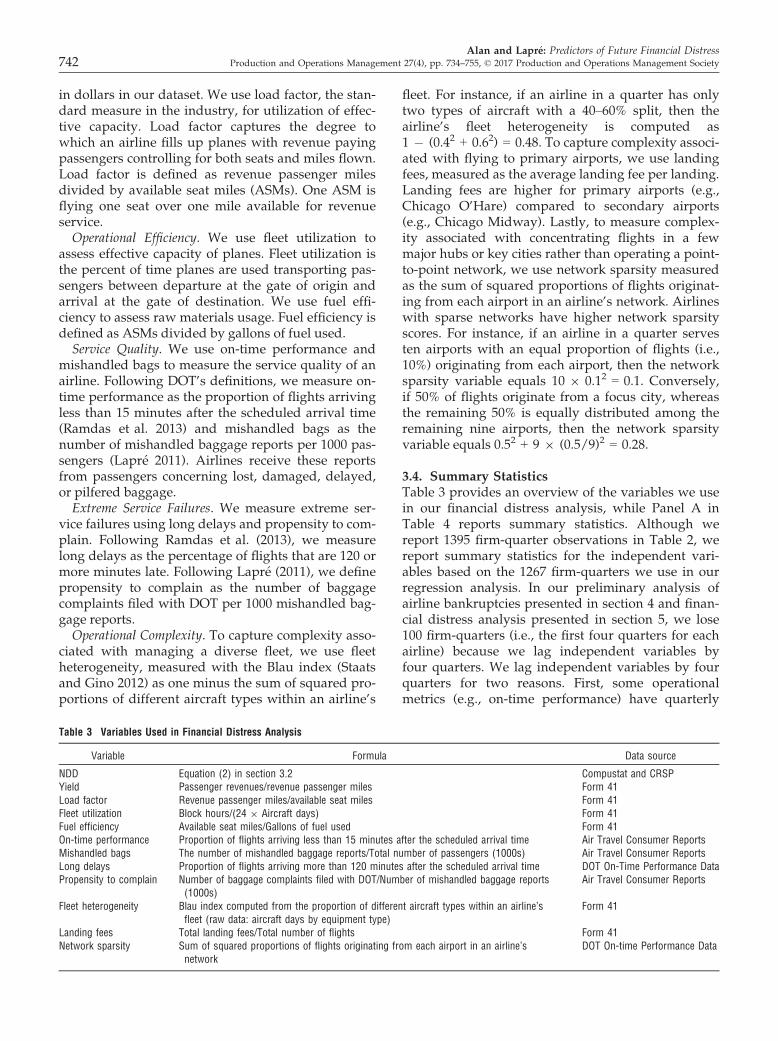
3.4. Summary StatisticsTable 3 provides an overview of the variables we usein our financial distress analysis, while Panel A inTable 4 reports summary statistics. Although wereport 1395 firm-quarter observations in Table 2, wereport summary statistics for the independent vari-ables based on the 1267 firm-quarters we use in ourregression analysis. In our preliminary analysis ofairline bankruptcies presented in section 4 and finan-cial distress analysis presented in section 5, we lose100 firm-quarters (i.e., the first four quarters for eachairline) because we lag independent variables byfour quarters. We lag independent variables by fourquarters for two reasons. First, some operationalmetrics (e.g., on-time performance) have quarterly

Table 3 Variables Used in Financial Distress Analysis

Variable Formula Data source

NDD Equation (2) in section 3.2 Compustat and CRSPYield Passenger revenues/revenue passenger miles Form 41Load factor Revenue passenger miles/available seat miles Form 41Fleet utilization Block hours/(24 9 Aircraft days) Form 41Fuel efficiency Available seat miles/Gallons of fuel used Form 41On-time performance Proportion of flights arriving less than 15 minutes after the scheduled arrival time Air Travel Consumer ReportsMishandled bags The number of mishandled baggage reports/Total number of passengers (1000s) Air Travel Consumer ReportsLong delays Proportion of flights arriving more than 120 minutes after the scheduled arrival time DOT On-Time Performance DataPropensity to complain Number of baggage complaints filed with DOT/Number of mishandled baggage reports

(1000s)Air Travel Consumer Reports

Fleet heterogeneity Blau index computed from the proportion of different aircraft types within an airline’sfleet (raw data: aircraft days by equipment type)

Form 41

Landing fees Total landing fees/Total number of flights Form 41Network sparsity Sum of squared proportions of flights originating from each airport in an airline’s

networkDOT On-time Performance Data


seasonality. Second, and more importantly, laggingoperational variables by four quarters eliminates apotential look-ahead bias and provides sufficienttime to airlines and regulators to take actions basedon the early warning signals the operational vari-ables generate. Moreover, section 6 shows that theoperational variables convey useful information up-to eight quarters before the measurement of financialdistress and thereby demonstrates the robustness ofour findings with respect to the time lag betweenoperational performance and future financialdistress.We lose 28 firm-quarters due to missing data. We

use all 1395 � (100 + 28) = 1267 firm-quarter obser-vations in our preliminary analysis presented in thenext section. However, we can calculate NDD and thecorresponding probability of bankruptcy for only1047 firm-quarters because stock price information isunavailable in firm-quarters during which an airlinewas either privately owned or operating under bank-ruptcy protection. Panel B in Table 4 shows the corre-lations among our variables. Because we lagindependent variables by four quarters in sections 4and 5, we report the correlations between na€ıve dis-tance to default and the four-quarter lagged values ofthe independent variables.

4. Preliminary Analysis of AirlineBankruptcies

In this section, we provide preliminary evidenceregarding the role of operational performance infinancial distress models. We test whether operational

characteristics can improve model fit in bankruptcyclassification analyses.

4.1. MethodologyModeling corporate bankruptcies has been an activeresearch domain in accounting, economics, andfinance since the early 1960s. A large body of litera-ture uses binary classification models to identifyfinancial ratios that explain corporate bankruptcies.In his seminal work, Altman (1968) applied multiplediscriminant analysis to a matched sample of bank-rupt and non-bankrupt firms to identify financialratios that capture a firm’s financial status. Becausethere are two distinct groups (bankrupt vs. non-bankrupt), the classification analysis can be trans-formed into a discriminant function of the formzn = bxn, where zn is the z-score for the nth observa-tion in the sample and xn is the corresponding vectorof firm specific variables. The goal is to estimate thecoefficient vector b such that every firm is correctlyidentified as bankrupt or non-bankrupt based on itsz-score.Altman (1968) identified five variables that perform

well in firm classification: working capital to totalassets (WC/TA), retained earnings to total assets(RE/TA), earnings before interest and taxes to totalassets (EBIT/TA), market value of equity to total lia-bilities (ME/TL), and sales to total assets (S/TA). In asubsequent study, Altman (1993) replaced ME/TLwith book value of equity to total liabilities (BE/TL),which facilitates the computation of a z-score for firmswithout stock price data. We use the independentvariables of this alternative model, known as the

Table 4 Summary Statistics and Correlation Matrix

Panel A Panel B

N Mean SD 1 2 3 4 5 6 7 8 9 10 11 12

1 NDD 1086 5.59 5.10 12 Yield 1267 13.16 3.86 0.00 13 Load factor 1267 0.73 0.08 �0.15 �0.58 14 Fleet utilization 1267 0.42 0.05 0.23 �0.42 0.13 15 Fuel Efficiency 1267 18.38 3.52 �0.14 0.70 �0.40 �0.60 16 On-time perf. 1267 0.79 0.06 0.20 �0.13 0.06 �0.08 �0.21 17 Mishandled bags 1267 5.50 2.56 �0.15 0.59 �0.30 �0.32 0.63 �0.42 18 Long delays 1267 0.01 0.01 �0.31 �0.15 0.40 0.09 0.06 �0.68 0.22 19 Prop. to complain 1267 0.43 0.48 �0.17 �0.16 0.02 0.00 �0.15 �0.04 �0.16 0.01 110 Fleet heterogeneity 1267 0.53 0.24 �0.35 0.22 �0.06 �0.33 0.17 �0.14 0.16 0.02 0.18 111 Landing fees 1267 270 151 �0.17 �0.39 0.24 0.20 �0.39 0.02 �0.35 0.04 0.48 0.25 112 Network sparsity 1267 0.10 0.05 �0.23 �0.33 0.33 0.13 �0.28 0.11 �0.13 0.02 0.09 �0.07 0.10 1

Notes. In Panel A, we present the number of observations, mean, and standard deviation (SD) for the na€ıve distance to default (NDD) and theindependent variables we use in our financial distress analyses presented in section 5 and 6. Na€ıve distance to default, fleet heterogeneity, and networksparsity are scalars. Yield and OR/ASM are expressed in 2000 US cents per seat mile. Load factor, fleet utilization, on-time performance, and long delaysare fractions. Fuel efficiency is expressed as miles per gallon. Mishandled bags are expressed as the number of mishandled baggage per 1000customers. Propensity to complain is expressed as the number of baggage complaints with DOT per 1000 mishandled bags. Landing fees are expressedin 2000 US dollars per landing. In Panel B, we report the correlation between na€ıve distance to default and the independent variables lagged by fourquarters used in our financial distress analyses presented in section 5 and 6. Because the independent variables shown in rows and columns 2–12 arelagged by four quarters, we report their contemporaneous pairwise correlations.


z0-score private firm model, in our first base model

because stock price data are unavailable for firm quar-ters during which the firm is in bankruptcy. Both zand z

0score models are still widely used by academics

and practitioners to assess a firm’s financial distress(Altman and Hotchkiss 2010).While Altman’s z and z

0scores are useful in terms

of identifying the financial ratios that explain corpo-rate bankruptcies, their model coefficients are typi-cally specified using a sample of firms from differentindustries. Thus, they may not be able to capturedynamics that are specific to the airline industry. Inorder to overcome this hurdle, researchers have pro-posed variables that are specific to the airline indus-try. One airline industry specific model is theAirscore model (Chow et al. 1991). The independentvariables of the Airscore model are market value ofequity to total liabilities (ME/TL), interest expense tototal liabilities (IE/TL), and operating revenues tototal miles flown (OR/TMF). Although the first twovariables of this model are generic, the last variable isindustry specific, and serves as a proxy for an airline’srevenue generation capabilities. We use the Airscoremodel’s independent variables in our second basemodel after replacing ME/TL with BE/TL so that wecan calculate an Airscore in the absence of stock priceinformation.We test four versions of the Altman’s z

0score model

in our preliminary analysis. Model 1 includes the Alt-man’s z

0score model’s independent variables, all

computed from Compustat data. Model 2 expandsthe set of independent variables of the z

0score model

by adding OR/ASM (which is yield 9 load factor),mishandled bags, fleet utilization, and fleet hetero-geneity. Model 3 expands Model 2 by adding a legacydummy that takes a value of 1 if airline i is a legacycarrier and 0 otherwise. Given that 14 out of 20 bank-ruptcy episodes presented in Table 2 belong to legacyairlines, Model 3 allows us to test whether operationalvariables are associated with bankruptcy classifica-tion rather than the higher financial distress of legacycarriers compared to low-cost carriers. Lastly, Model4 has the same independent variables as Model 3, butexcludes Southwest. Comparing Model 4 with Model3 allows us to check whether our findings are drivenby the superior operational and financial performanceof Southwest. We follow a similar approach with fourversions of the Airscore model: Models 5–8. We com-pute the Airscore model’s independent variables BE/TL and IE/TL from Compustat data and OR/TMFfrom Form 41 data.The discriminant analysis approach can be con-

sidered as a single period model that uses only oneobservation from each firm (typically the last obser-vation in the data). Shumway (2001) demonstratesthat this approach leads to biased and inconsistent

coefficient estimates due to its static nature, over-looking data on healthy firms that eventually gobankrupt. A more appropriate approach is a dura-tion model (also known as a hazard model), whichcaptures the dynamic nature of bankruptcy risk.Shumway (2001) and Chava and Jarrow (2004) showthat the likelihood function of a discrete-time haz-ard model is identical to that of a multi-period logitmodel and that a discrete-time hazard model can beestimated via logistic regression. We adopt the sameapproach and seek to classify firm-quarter observa-tions via logistic regression. In the logit model,PrðBankruptit ¼ 1Þ ¼ 1

1þexpð�bXi;t�4Þ, where Xi,t�4

denotes the vector of independent variables laggedby four quarters.

4.2. ResultsTable 5 shows the results of our preliminary bank-ruptcy analysis. All independent variables exceptWC/TA are significant at p = 0.05 in Model 1. Consis-tent with Altman’s findings, we find that lower RE/TA, EBIT/TA, BE/TL, and S/TA are associated withhigher future financial distress. The insignificance ofWC/TA is consistent with Shumway (2001), who doc-uments the insignificance of this variable using abroader sample of firms.A likelihood ratio test between Models 1 and 2 has

a p-value of 0.002. So, adding revenue management,operational efficiency, service quality, and opera-tional complexity to the Altman’s z

0score model

leads to a statistically significant improvement inmodel fit. Model 2 indicates that lower operatingrevenue per ASM, lower fleet utilization, and higherfleet heterogeneity are associated with higher futurefinancial distress. Despite having the correct sign,mishandled bags is statistically insignificant. Replac-ing mishandled bags with propensity to complaindoes not change our results. A likelihood ratio testbetween Models 2 and 3 has a p-value of 0.247, indi-cating that controlling for the low-cost–legacy differ-ence does not improve model fit. A comparison ofthe estimates of Models 2 and 3 reveals that theaddition of the legacy fixed effect does not changethe statistical significance (or insignificance) ofModel 2’s independent variables. Moreover, thelegacy fixed effect is statistically insignificant inModel 3. The estimates of Model 4, which excludesSouthwest, are qualitatively similar to Model 3. Esti-mating the Airscore model leads to similar insights(Models 5–8).Our preliminary analysis shows that operational

performance metrics can improve goodness of fit inbankruptcy classification models and that thisimprovement is not driven by the low-cost–legacy dif-ference or a Southwest effect. In particular, we findsupport for Hypotheses 1, 2, and 4, whereas we do


not find a link between service quality (Hypothesis3A) or extreme service failures (Hypothesis 3B) andbankruptcy in subsequent quarters.

4.3. LimitationsDespite their widespread use in the airline bank-ruptcy literature (e.g., Chow et al. 1991, Gritta et al.2008, Lu et al. 2015), binary classification models havesome significant limitations. First, bankruptcy is anextreme form of financial distress. By labeling airlinesas bankrupt vs. non-bankrupt, binary classificationmodels may not distinguish between healthy airlinesand airlines that are on the verge of bankruptcy.Moreover, out-of-sample evidence is necessary toestablish the empirical reliability of a forecastingmodel (Rapach et al. 2010). However, the binary clas-sification models in the airline industry rely on a

small number of bankruptcy filings, which preventsresearchers from testing the out-of-sample forecastaccuracy. Consequently, inferences from binary clas-sification models regarding the association betweenoperational performance and future financial distressmay be inaccurate.Second, a general rule of thumb in logistic regres-

sion is to have at least 10 events per parameter inorder to have reliable parameter estimates (Hosmerand Lemeshow 2004). Because we only have 120bankrupt quarters in our logistic regression sample,we should have fewer than 12 independent variables.Therefore, we attempt to capture the associationbetween each area of operational performance andfuture financial distress with only variable (e.g., OR/ASM to proxy revenue management) rather thanusing multiple variables (e.g., yield and load factor).

Table 5 Logistic Regression Results

Altman’s z0model Airscore model

Model 1 Model 2 Model 3 Model 4 Model 5 Model 6 Model 7 Model 8

(Intercept) �1.726*** 1.910 2.003 2.071 �0.718 1.601 1.786 1.789(0.292) (1.704) (1.704) (1.703) (0.541) (1.362) (1.366) (1.364)

WC/TA 0.696 0.965 0.899 0.827(0.833) (0.938) (0.935) (0.942)

RE/TA �3.289*** �3.596*** �3.692*** �3.703***(0.589) (0.609) (0.624) (0.623)

EBIT/TA �17.940*** �12.905** �13.384** �13.321**(4.133) (4.526) (4.532) (4.523)

BE/TL �1.396* �0.922 �0.974 �0.910 �3.676*** �3.508*** �3.397*** �3.378***(0.578) (0.571) (0.575) (0.584) (0.390) (0.402) (0.412) (0.415)

S/TA �2.837** �3.231** �3.482** �3.523**(0.995) (1.189) (1.221) (1.222)

OR/ASM �0.237*** �0.230** �0.230**(0.071) (0.071) (0.071)

Fleet utilization �6.417* �6.727* �6.716* �6.080* �5.712* �5.680*(3.019) (3.017) (3.002) (2.788) (2.806) (2.802)

Mishandled bags 0.065 0.068 0.066 0.063 0.065 0.065(0.054) (0.053) (0.053) (0.050) (0.051) (0.051)

Fleet heterogeneity 1.353* 1.766* 1.662* 3.175*** 2.713*** 2.680***(0.680) (0.776) (0.791) (0.688) (0.779) (0.784)

IE/TL 45.343* 37.248 33.891 33.700(21.742) (22.728) (23.035) (23.029)

OR/TMF �1.032** �2.463*** �2.698*** �2.693***(0.356) (0.455) (0.499) (0.499)

Legacy �0.359 �0.348 0.405 0.410(0.308) (0.308) (0.339) (0.339)

# of airlines 25 25 25 24 25 25 25 24# of observations 1267 1267 1267 1167 1267 1267 1267 1167# of bankrupt qtrs. 120 120 120 120 120 120 120 120# of non-bankrupt qtrs. 1147 1147 1147 947 1147 1147 1147 947AIC 620.128 611.310 611.969 611.340 657.502 634.738 635.281 635.070BIC 743.594 817.086 838.323 834.077 739.813 778.782 799.902 797.061Pseudo R2 0.293 0.317 0.319 0.301 0.231 0.264 0.277 0.255Log likelihood �304.064 �295.655 �294.984 �294.670 �324.751 �310.369 �309.641 �309.535Likelihood ratio test 16.819 (p = 0.002) 28.764 (p < 10�3)Likelihood ratio test 1.341 (p = 0.247) 1.457 (p = 0.227)

Notes. Standard errors in parentheses. *, **, and *** indicate statistical significance at 0.05, 0.01, and p = 0.001, respectively. The dependent variable isBankruptit. All explanatory variables except the legacy dummy are lagged by four quarters. We perform parameter estimation via logistic regression. InModels 4 and 8, we drop the Southwest observations.


Furthermore, we cannot introduce parameters to cap-ture airline or time specific effects that may influencefinancial distress. Not being able to incorporate fixedeffects impedes the reliability of inferences in indus-try-specific studies (Joglekar et al. 2016). For instance,we do not find support for Hypothesis 3B (extremeservice failures) in our preliminary analysis of airlinebankruptcies, but we do find support for this hypoth-esis in the next section, where we control for airlineand time specific effects.Lastly, as discussed in Phillips and Sertsios (2013),

the weights assigned to each financial ratio (i.e., theestimated coefficients of each financial ratio) can bequite unstable in a binary classification model becauseof industry trends that systematically change thoseratios. As a result, the estimated z–scores can be unre-liable. In the next section, we overcome these hurdlesby replacing the binary classification with a continu-ous financial distress metric. Consequently, we can (i)distinguish between healthy airlines and financiallydistressed but non-bankrupt airlines, (ii) jointly testthe significance of a relatively large number of inde-pendent variables, and (iii) perform out-of-sampleforecasts.

5. Financial Distress Analysis

In this section, we examine the association betweenoperational performance and future financial distress.Section 5.1 explains our methodology, and section 5.2discusses our results and robustness of our findings.

5.1. MethodologyOur model specification has the following form:

�NDDit ¼ ai þ ct þXk

bkxk;i;t�4 þ h �NDDi;t�4

� �þ uit;

ð3Þwhere ai is the airline dummy, ct is the timedummy, xk,i,t�4 are the lagged values of operationalvariables, and uit is the error term. We use�1 9 NDD (rather than NDD) as our dependentvariable to ensure that the estimated coefficientsigns are consistent with the ones we obtained insection 4.Many economic and financial variables dynami-

cally evolve over time. In empirical settings, dynamicrelationships are captured by the presence of a laggeddependent variable among the independent variables.(See Baltagi (2008, ch. 8) for an overview of dynamicpanel data models and their applications in eco-nomics.) Accordingly, we use �NDDi,t�4 as an inde-pendent variable to capture the dynamic nature offinancial distress. Another reason to use �NDDi,t�4 asan independent variable is a potential link between

an airline’s financial distress state and operationalperformance. A financially distressed airline couldalso anticipate financial distress in future periods andthereby take actions that could influence our opera-tional predictors. For instance, a financially distressedairline could lower its ticket prices, reduce its capac-ity, downsize its flight networks, and/or lower its ser-vice quality to improve its short-term liquidity.Including �NDDi,t�4 allows us to test whether opera-tional performance is associated with future financialdistress after controlling for an airline’s financialdistress state at the time we measure operationalperformance.We test seven models. Model 1 is the base model

with airline and time dummies. Model 2 expandsModel 1 by adding yield, load factor, on-time perfor-mance, mishandled bags, fleet utilization, fuelefficiency, fleet heterogeneity, landing fees, and net-work sparsity. Model 3 expands Model 2 by addingNDDi,t�4. To test whether our findings are driven bythe superior operational and financial performance ofSouthwest, Model 4 has the same independent vari-ables as Model 3, but excludes Southwest. In Models5–7, we replace the service quality variables in Models2–4 (on-time performance and mishandled bags) withthe extreme service failure variables (long delays andpropensity to complain).Models 1, 2, 3, 5, and 6 have 25 airlines, whereas

Models 4 and 7 have 24 airlines due to the exclusionof Southwest. The number of quarters per airline var-ies from 3 to 100 in all seven models. Thus, we haveunbalanced time-series cross-section (TSCS) data,which is different from panel data (Beck 2001). Inpanel data, the asymptotics are in the number ofunits. In TSCS data, the units are fixed, there is nosampling, and we are interested in specific units. Theasymptotics are in time periods. Consequently, theestimation method needs to deal with panelheteroskedasticity (E½u2it� ¼ r2i 6¼ E½u2jt� ¼ r2j fori 6¼ j), contemporaneous correlation (E[uitujt] = rij),and autocorrelation (uit = qiui,t�1 + eit).

2 FollowingBeck and Katz (1995), we use Prais–Winstein regres-sion with a single first-order autoregressive processcommon to all airlines and estimate panel-correctedstandard errors, which account for panel hetero-skedasticity and contemporaneous correlation.3 Otherairline industry studies that use our estimationmethodology include Lapr�e and Tsikriktsis (2006)and Lapr�e (2011).

5.2. ResultsTable 6 shows the regression results. Models 1explains 57.6% of the variation in financial distress,whereas Model 2 explains 61.3%. Both revenuemanagement variables, yield and load factor, are neg-atively associated with future financial distress.


Among the operational efficiency variables, fleetutilization is negative and significant, whereas fuelefficiency is statistically insignificant. Both ser-vice quality variables, on-time performance and mis-handled bags, are statistically insignificant at p = 0.05.All three operational complexity variables (fleetheterogeneity, landing fees, and network sparsity) arestatistically significant with the expected signs. Model3 explains 64.8% of variation in financial distress. Thelagged value of NDD is significant indicating that thecurrent financial distress state is an important deter-minant of the future distress state. The addition of thelagged NDD in Model 3 does not change the signifi-cance findings for the operational variables in Model2. The coefficient estimates of Model 4, whichexcludes Southwest, are qualitatively similar to thoseof Model 3 indicating that our findings are not drivenby the superior operational and financial performanceof Southwest.Model 5 explains 62.4% of the variation in financial

distress. Unlike service quality variables, extreme

service failure variables are significant. Both longdelays and propensity to complain are positivelyassociated with future financial distress. Replacingservice quality with extreme service failures does notchange the significance findings for the other opera-tional variables in Model 2. Model 6 explains 65.6% ofthe variation in financial distress. Lagged NDD is sig-nificant. The addition of the lagged NDD does notchange the significance findings in Model 5 for theoperational variables. Lastly, the estimates of Model7, which excludes Southwest, are qualitatively similarto Model 6.In sum, our findings from Models 1–7 are consis-

tent. We find support for Hypothesis 1, i.e., lower val-ues of yield and load factor are associated with higherfuture financial distress. We find partial support forHypothesis 2, as low fleet utilization is associatedwith higher future financial distress, whereas fuelefficiency is not significant. The insignificance of fuelefficiency is primarily driven by the lack of contempo-raneous heterogeneity among airlines. In a given

Table 6 Financial Distress Regression Results

Average service quality Extreme service failures

Model 1 Model 2 Model 3 Model 4 Model 5 Model 6 Model 7

Yield �0.314*** �0.277*** �0.240*** �0.311*** �0.275*** �0.241***(0.072) (0.067) (0.065) (0.071) (0.066) (0.065)

Load factor �10.569* �9.354* �11.884** �11.559** �9.967* �12.320**(4.484) (4.387) (4.256) (4.408) (4.314) (4.158)

Fleet utilization �12.071* �12.766** �10.897* �12.954* �13.373** �11.024*(5.169) (4.895) (4.791) (5.127) (4.859) (4.756)

Fuel efficiency 0.084 0.070 0.039 0.050 0.043 0.015(0.081) (0.077) (0.078) (0.081) (0.078) (0.079)

On-time perf. �0.029 �0.028 �0.026(0.026) (0.026) (0.025)

Mishandled bags �0.161 �0.155 �0.137(0.097) (0.091) (0.092)

Long delays 48.528** 41.955* 40.837*(17.851) (17.820) (17.821)

Prop. to complain 1.287** 1.208** 1.253**(0.407) (0.402) (0.392)

Fleet heterogeneity 4.294** 3.473** 3.574** 3.679* 2.937* 2.989*(1.450) (1.309) (1.331) (1.432) (1.307) (1.330)

Landing fees 0.011*** 0.010** 0.007* 0.011*** 0.009** 0.007*(0.003) (0.003) (0.003) (0.003) (0.003) (0.003)

Network sparsity 27.450** 24.706** 16.233* 26.495** 23.649** 15.673*(8.441) (7.683) (7.750) (8.284) (7.622) (7.766)

Lagged NDD 0.190*** 0.177*** 0.180*** 0.166***(0.038) (0.038) (0.038) (0.038)

# of airlines 25 25 25 24 25 25 24# of observations 1047 1047 1047 947 1047 1047 947R2 0.576 0.613 0.648 0.600 0.624 0.656 0.608Autocor. coeff., q 0.512 0.437 0.360 0.369 0.419 0.351 0.361

Notes. The dependent variable is �NDDit. All independent variables are lagged by four quarters. Because �NDDi,t�4 is unavailable in 39 firm-quarters,Models 1, 2, 3, 5, and 6 have 1086�39 = 1047 observations. Because Models 4 and 7 exclude Southwest, they have 24 airlines and 947 observations.All models have airline and time dummies. We do not report the coefficient estimates for airline and quarter dummies due to space limitations. Weperform parameter estimation via Prais-Winsten regression with panel-corrected standard errors and a single first-order autoregressive process commonto all airlines, i.e., uit = qui,t�1 + eit. Panel-corrected standard errors, which correct for panel heteroskedasticity and contemporaneous correlation, are inparentheses. *, **, and *** indicate statistical significance at 0.05, 0.01, and 0.001, respectively.


quarter, there is very little variation among airlines interms of their fuel efficiencies. We do not find supportfor Hypothesis 3A. Service quality, measured by on-time performance and mishandled bags, does nothave a significant association with future financialdistress. However, we do find support for Hypothesis3B. Extreme service failures are associated withhigher future financial distress. Lastly, we find sup-port for Hypothesis 4 as fleet heterogeneity, landingfees, and network sparsity are associated with higherfuture financial distress.We conducted several tests to assess the robustness

of our findings. Recall from section 3 that when a cor-poration owns more than one airline in the sample,we use the parent company’s NDD for all airlinesowned by that company. We test the robustness ofour findings by replicating Models 1–7 on a smallersample in which we only keep the largest airlineowned by the parent company. Our findings regard-ing the associations between four operational dimen-sions and future financial distress remainedunchanged in the smaller sample. In addition, wetested different versions of our models with only onevariable for each operational dimension. For instance,we used either on-time performance or mishandledbags to measure service quality. The impact of rev-enue management, operational efficiency, servicequality (or extreme service failures), and operationalcomplexity remained qualitatively unchanged underthose alternative specifications. Furthermore, we

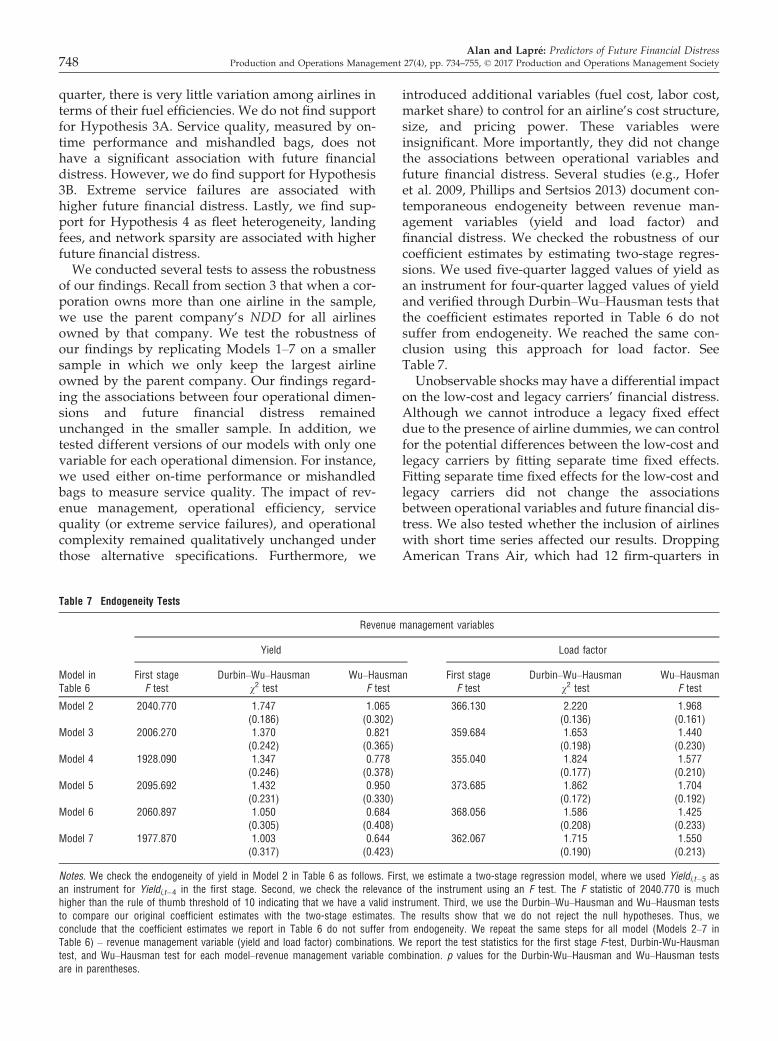
introduced additional variables (fuel cost, labor cost,market share) to control for an airline’s cost structure,size, and pricing power. These variables wereinsignificant. More importantly, they did not changethe associations between operational variables andfuture financial distress. Several studies (e.g., Hoferet al. 2009, Phillips and Sertsios 2013) document con-temporaneous endogeneity between revenue man-agement variables (yield and load factor) andfinancial distress. We checked the robustness of ourcoefficient estimates by estimating two-stage regres-sions. We used five-quarter lagged values of yield asan instrument for four-quarter lagged values of yieldand verified through Durbin–Wu–Hausman tests thatthe coefficient estimates reported in Table 6 do notsuffer from endogeneity. We reached the same con-clusion using this approach for load factor. SeeTable 7.Unobservable shocks may have a differential impact

on the low-cost and legacy carriers’ financial distress.Although we cannot introduce a legacy fixed effectdue to the presence of airline dummies, we can controlfor the potential differences between the low-cost andlegacy carriers by fitting separate time fixed effects.Fitting separate time fixed effects for the low-cost andlegacy carriers did not change the associationsbetween operational variables and future financial dis-tress. We also tested whether the inclusion of airlineswith short time series affected our results. DroppingAmerican Trans Air, which had 12 firm-quarters in

Table 7 Endogeneity Tests

Revenue management variables

Yield Load factor

Model inTable 6

First stageF test

Durbin–Wu–Hausmanv2 test

Wu–HausmanF test

First stageF test

Durbin–Wu–Hausmanv2 test

Wu–HausmanF test

Model 2 2040.770 1.747 1.065 366.130 2.220 1.968(0.186) (0.302) (0.136) (0.161)

Model 3 2006.270 1.370 0.821 359.684 1.653 1.440(0.242) (0.365) (0.198) (0.230)

Model 4 1928.090 1.347 0.778 355.040 1.824 1.577(0.246) (0.378) (0.177) (0.210)

Model 5 2095.692 1.432 0.950 373.685 1.862 1.704(0.231) (0.330) (0.172) (0.192)

Model 6 2060.897 1.050 0.684 368.056 1.586 1.425(0.305) (0.408) (0.208) (0.233)

Model 7 1977.870 1.003 0.644 362.067 1.715 1.550(0.317) (0.423) (0.190) (0.213)

Notes. We check the endogeneity of yield in Model 2 in Table 6 as follows. First, we estimate a two-stage regression model, where we used Yieldi,t�5 asan instrument for Yieldi,t�4 in the first stage. Second, we check the relevance of the instrument using an F test. The F statistic of 2040.770 is muchhigher than the rule of thumb threshold of 10 indicating that we have a valid instrument. Third, we use the Durbin–Wu–Hausman and Wu–Hausman teststo compare our original coefficient estimates with the two-stage estimates. The results show that we do not reject the null hypotheses. Thus, weconclude that the coefficient estimates we report in Table 6 do not suffer from endogeneity. We repeat the same steps for all model (Models 2–7 inTable 6) – revenue management variable (yield and load factor) combinations. We report the test statistics for the first stage F-test, Durbin-Wu-Hausmantest, and Wu–Hausman test for each model–revenue management variable combination. p values for the Durbin-Wu–Hausman and Wu–Hausman testsare in parentheses.


our models after dropping the first four quarters dueto lagging, Independence Air (8 firm-quarters), andPiedmont Aviation (3 firm-quarters) did not changeour findings. Lastly, in case an airline declaredbankruptcy, exited bankruptcy, and started tradinglater, we fitted separate firm dummies for pre- andpost-bankruptcy quarters, which allows us to treatthe pre- and post-bankruptcy episodes as twoseparate firms. Once again, our findings remainedunchanged.

6. Out-of-Sample Forecasts of FutureFinancial Distress

In this section, we switch our focus from testing asso-ciations to generating out-of-sample forecasts toinvestigate whether operational performance can beused to predict future financial distress. Section 6.1explains our methodology, and section 6.2 presentsour findings.

6.1. MethodologyWe generate out-of-sample forecasts of NDD usinga recursive estimation window for different lags.Recursive forecasting models are commonly usedin economics and finance to test the predictiveability of a variable of interest (e.g., Goyal andWelch 2003, Rapach et al. 2010, and referencestherein). To test of the robustness of our findings,we perform sensitivity analyses with different lagperiods.In order to generate out-of-sample forecasts, we

first divide our study period of 104 quarters into anin-sample portion consisting of the first 40 quarters(from the first quarter of 1988 until the last quarter of1997) and an out-of-sample portion consisting of thelast 64 quarters (from the first quarter of 1998 until thelast quarter of 2013). We generate out-of-sample fore-casts for the first quarter of 1998 (i.e., t = 41) as fol-lows. Let l denote the time lag between theoperational variables and future financial distress. Forl = 1, ⋯, 8, we use data from the first 40 quarters andthe estimation methodology described in section 5 toestimate the coefficients of the model specificationdescribed as Model 6 in section 5 as

�NDDis ¼ a½OM;40;l�i þ c½OM;40;l�

s þXk

b½OM;40;l�k xk;i;s�l

� h½OM;40;l�NDDi;s�l þ u½OM;40;l�is ;

ð4Þwhere s 2 {5, ⋯, 40} and the superscript [OM, 40, l]indicates that we estimate the coefficients of anoperational performance model (OM) using datafrom the first 40 quarters. Then, for l = 1, ⋯, 8, we

predict na€ıve distance to default for airline i att = 41, dNDD

½OM;l�i;41 , as

dNDD½OM;l�i;41 ¼ �

ba½OM;40;l�i þ bc½OM;40;l�

41�l

þXk

bb½OM;40;l�k xk;i;41�l � bh½OM;40;l�NDDi;41�l

!;

ð5Þ

where ba½OM;40;l�i , bc½OM;40;l�

41�l , bb½OM;40;l�k , and bh½OM;40;l�

denote the coefficient estimates. Because we esti-mate model coefficients of equation (4) using datafrom the first 40 quarters, and because the right-hand side of equation (5) has the lagged values ofindependent variables, dNDD

½OM;l�i;41 is an out-of-sam-

ple forecast.We generate out-of-sample forecasts for the remain-

ing quarters of the out-of-sample portion of our datain a recursive manner. Specifically, in order to gener-ate forecasts for quarter t = 41, ⋯, 104, we first esti-mate the coefficients of the model specified inequation (4) using data up to quarter t � 1. We thenuse the estimated model coefficients, ba½OM;t�1;l�

i ,bc½OM;t�1;l�t�l , bb½OM;t�1;l�

k , and bh½OM;t�1;l�, and calculate aone-step ahead forecast for airline i at lag l and time tas

dNDD½OM;l�i;t ¼ �

ba½OM;t�1;l�i þ bc½OM;t�1;l�

t�l

þXk

bb½OM;t�1;l�k xk;i;t�l � bh½OM;t�1;l�NDDi;t�l

!:

ð6ÞGiven the observed distance to default, NDDit, and

the corresponding forecast, dNDD½OM;l�it , we calculate

the forecast error of our model for airline i at lag l andtime t as

e½OM;l�it ¼ N �NDDitð Þ � N � dNDD

½OM;l�it

� �: ð7Þ

We calculate forecast errors based on the observedand predicted bankruptcy probabilities (rather thanthe observed and predicted distance to default val-ues) because forecast errors are easier to interpret inthe probability domain as they lie in the interval[�1, 1]. For each lag (l = 1, ⋯, 8), we compare theperformance of our forecasting model with a bench-mark model.Our benchmark model combines the Altman vari-

ables with the lagged value of NDD. Using data up toperiod t � 1, we first fit the following benchmarkmodel (BM):


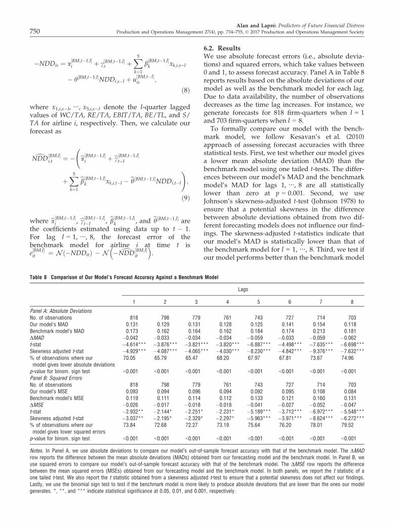
�NDDis ¼ a½BM;t�1;l�i þ c½BM;t�1;l�

s þX5k¼1

b½BM;t�1;l�k xk;i;s�l

� h½BM;t�1;l�NDDi;s�l þ u½BM;t�l�is ;

ð8Þ

where x1,i,s�l, ⋯, x5,i,s�l denote the l-quarter laggedvalues of WC/TA, RE/TA, EBIT/TA, BE/TL, and S/TA for airline i, respectively. Then, we calculate ourforecast as

dNDD½BM;l�i;t ¼ �

ba½BM;t�1;l�i þ bc½BM;t�1;l�

t�l

þX5k¼1

bb½BM;t�1;l�k xk;i;t�l � bh½BM;t�1;l�NDDi;t�l

!;

ð9Þ

where ba½BM;t�1;l�i , bc½BM;t�1;l�

t�l , bb½BM;t�1;l�k , and bh½BM;t�1;l� are

the coefficients estimated using data up to t � 1.For lag l = 1, ⋯, 8, the forecast error of thebenchmark model for airline i at time t ise½BM;l�it ¼ N �NDDitð Þ � N � dNDD

½BM;l�it

� �.

6.2. ResultsWe use absolute forecast errors (i.e., absolute devia-tions) and squared errors, which take values between0 and 1, to assess forecast accuracy. Panel A in Table 8reports results based on the absolute deviations of ourmodel as well as the benchmark model for each lag.Due to data availability, the number of observationsdecreases as the time lag increases. For instance, wegenerate forecasts for 818 firm-quarters when l = 1and 703 firm-quarters when l = 8.To formally compare our model with the bench-

mark model, we follow Kesavan’s et al. (2010)approach of assessing forecast accuracies with threestatistical tests. First, we test whether our model givesa lower mean absolute deviation (MAD) than thebenchmark model using one tailed t-tests. The differ-ences between our model’s MAD and the benchmarkmodel’s MAD for lags 1, ⋯, 8 are all statisticallylower than zero at p = 0.001. Second, we useJohnson’s skewness-adjusted t-test (Johnson 1978) toensure that a potential skewness in the differencebetween absolute deviations obtained from two dif-ferent forecasting models does not influence our find-ings. The skewness-adjusted t-statistics indicate thatour model’s MAD is statistically lower than that ofthe benchmark model for l = 1, ⋯, 8. Third, we test ifour model performs better than the benchmark model

Table 8 Comparison of Our Model’s Forecast Accuracy Against a Benchmark Model

Lags

1 2 3 4 5 6 7 8

Panel A: Absolute DeviationsNo. of observations 818 798 779 761 743 727 714 703Our model’s MAD 0.131 0.129 0.131 0.128 0.125 0.141 0.154 0.118Benchmark model’s MAD 0.173 0.162 0.164 0.162 0.184 0.174 0.213 0.181DMAD �0.042 �0.033 �0.034 �0.034 �0.059 �0.033 �0.059 �0.062t-stat �4.614*** �3.876*** �3.821*** �3.820*** �6.887*** �4.498*** �7.635*** �6.698***Skewness adjusted t-stat �4.929*** �4.087*** �4.065*** �4.030*** �8.230*** �4.842*** �9.376*** �7.632***% of observations where ourmodel gives lower absolute deviations

70.05 65.79 65.47 68.20 67.97 67.81 73.67 74.96

p-value for binom. sign test <0.001 <0.001 <0.001 <0.001 <0.001 <0.001 <0.001 <0.001Panel B: Squared ErrorsNo. of observations 818 798 779 761 743 727 714 703Our model’s MSE 0.093 0.094 0.096 0.094 0.092 0.095 0.108 0.084Benchmark model’s MSE 0.119 0.111 0.114 0.112 0.133 0.121 0.160 0.131DMSE �0.026 �0.017 �0.018 �0.018 �0.041 �0.027 �0.052 �0.047t-stat �2.932** �2.144* �2.251* �2.231* �5.189*** �3.712*** �6.972*** �5.548***Skewness adjusted t-stat �3.037** �2.195* �2.329* �2.297* �5.963*** �3.971*** �8.624*** �6.272***% of observations where ourmodel gives lower squared errors

73.84 72.68 72.27 73.19 75.64 76.20 78.01 79.52

p-value for binom. sign test <0.001 <0.001 <0.001 <0.001 <0.001 <0.001 <0.001 <0.001

Notes. In Panel A, we use absolute deviations to compare our model’s out-of-sample forecast accuracy with that of the benchmark model. The DMADrow reports the difference between the mean absolute deviations (MADs) obtained from our forecasting model and the benchmark model. In Panel B, weuse squared errors to compare our model’s out-of-sample forecast accuracy with that of the benchmark model. The DMSE row reports the differencebetween the mean squared errors (MSEs) obtained from our forecasting model and the benchmark model. In both panels, we report the t statistic of aone tailed t-test. We also report the t statistic obtained from a skewness adjusted t-test to ensure that a potential skewness does not affect our findings.Lastly, we use the binomial sign test to test if the benchmark model is more likely to produce absolute deviations that are lower than the ones our modelgenerates. *, **, and *** indicate statistical significance at 0.05, 0.01, and 0.001, respectively.


for more than half of the forecasts (e.g., if it gives alower absolute deviation for more than 818/2 = 409data points when l = 1). We perform this analysisusing a non-parametric binomial sign test. Ourmodel generates lower absolute deviations than thebenchmark model. The difference from 50% is statis-tically significant at p = 0.001 for all l = 1, ⋯, 8.Panel B in Table 8 reports results based on thesquared errors of our model as well as the bench-mark model for each lag, l = 1, . . ., 8. Performingforecast comparisons between our model and thebenchmark model based on squared errors does notchange our findings.Our analyses indicate that our model is more

likely to generate smaller forecast errors than thebenchmark model, on average. Similarly, our non-parametric analyses show that for a randomly pickedfirm-quarter observation, our model is more likely togenerate a more accurate forecast than the bench-mark model. These results are robust to the time lagbetween predictive variables and future financial dis-tress. Thus, we conclude that operational perfor-mance can contribute to predicting future financialdistress.

7. Managerial Insights

Our findings suggest that airlines and outside stake-holders (e.g., regulators) can use operational perfor-mance to generate early warning signals regardingfuture financial distress. Additionally, our empiricalmodel can be used for comparative purposes. To fur-ther illustrate these ideas, we compare and contrastfour major players in the US airline industry, Ameri-can, Delta, JetBlue, and Southwest, in terms of theirfinancial distress and ability to manage key opera-tional variables post 9/11. The US airline industryexperienced a major shock from the terrorist attacksof September 11, 2001. Figure 1 shows that the aver-age bankruptcy probability exceeded 0.50 for severalquarters after 9/11, primarily due to high volatilityand steep declines in stock prices. Both American andDelta felt the negative impact immediately with theirstock prices declining more than 35% within a weekof the attacks. While most carriers were downsizingtheir workforce and flight schedules after 9/11,Southwest and JetBlue did the opposite by movinginto markets deserted by their competitors. Shortlyafter 9/11, Southwest became the third airline afterAmerican and Delta in terms of the number ofenplaned passengers, and JetBlue gained major airlinestatus. In light of these observations, we examineAmerican, Delta, JetBlue, and Southwest during theperiod 2005–2013. Starting in 2005 enables us toexclude the industry-wide effect of 9/11 observed fora few years after the attacks and examine JetBlue after

it obtained a relatively large market share in theindustry.Figure 2 shows the average probability of bank-

ruptcy for airlines between 2005 Q1 and 2013 Q4.Southwest is clearly superior to its competitors interms of financial stability. Its average probability ofbankruptcy is less than 0.01. JetBlue also has a rela-tively low average bankruptcy probability of 0.04,whereas the average bankruptcy probabilities equal0.23 and 0.15 for American and Delta, respectively.Our empirical model specification (equation 3)implies a non-linear relationship between operationalvariables and the probability of bankruptcy, becausewe transform NDD to Nð�NDDÞ. Consequently, ourbankruptcy probability estimates are more sensitiveto operational performance for airlines with distanceto default values between �2 and 2. As illustrated inFigure 2, the slope of the bankruptcy probabilitycurve is steepest in this range.Figure 3 shows how four operational variables

yield, load factor, fleet utilization, and fleet hetero-geneity affect bankruptcy probability estimates. Fig-ure 3a captures the sensitivity of our estimates toyield. We generate Figure 3a by using the coefficientestimates of Model 6 reported in Table 6. Estimatingairline fixed effects enables to us derive a separatebankruptcy probability curve for each airline. We esti-mate bankruptcy probabilities by replacing the actualvalue of yield with numerous yield values varyingbetween 7 and 14 ¢/ASM while keeping the originalvalues of the remaining explanatory variables. (Seethe notes to Figure 3 for the details of our methodol-ogy.) Although high yield is associated with lower

−4 −2 0 2 4

0.0

0.2

0.4

0.6

0.8

1.0

−Naive distance to default

Ave

rage

Pr(

Ban

krup

tcy)

AmericanDeltaJetBlueSouthwestOther Airlines

Figure 2 The Average Probability of Bankruptcy and the CorrespondingNa€ıve Distance to Default by Airline Between 2005 Q1 and2013 Q4

Notes. We compute the probability of bankruptcy for airline i in quarter tusing Bharath and Shumway’s (2008) na€ıve distance to default, NDDmetric. We compute the average probability of bankruptcy for airline i bytaking a simple average over all quarters in which the airline was publiclytraded between the first quarter of 2005 and the last quarter of 2013. Weplot �1 9 NDD on the x-axis to be consistent with our regression modelspecifications.


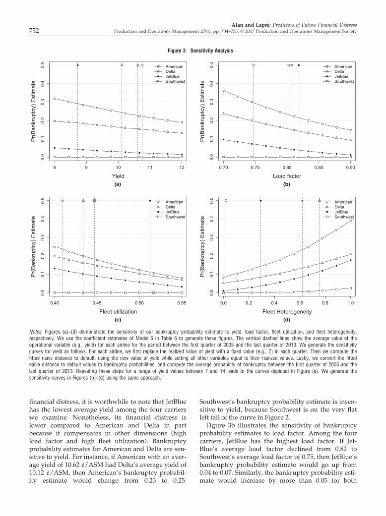
financial distress, it is worthwhile to note that JetBluehas the lowest average yield among the four carrierswe examine. Nonetheless, its financial distress islower compared to American and Delta in partbecause it compensates in other dimensions (highload factor and high fleet utilization). Bankruptcyprobability estimates for American and Delta are sen-sitive to yield. For instance, if American with an aver-age yield of 10.62 ¢/ASM had Delta’s average yield of10.12 ¢/ASM, then American’s bankruptcy probabil-ity estimate would change from 0.23 to 0.25.

Southwest’s bankruptcy probability estimate is insen-sitive to yield, because Southwest is on the very flatleft tail of the curve in Figure 2.Figure 3b illustrates the sensitivity of bankruptcy

probability estimates to load factor. Among the fourcarriers, JetBlue has the highest load factor. If Jet-Blue’s average load factor declined from 0.82 toSouthwest’s average load factor of 0.75, then JetBlue’sbankruptcy probability estimate would go up from0.04 to 0.07. Similarly, the bankruptcy probability esti-mate would increase by more than 0.05 for both

8 9 10 11 12

0.0

0.1

0.2

0.3

0.4

0.5

Yield

Pr(

Ban

krup

tcy)

Est

imat

e

(a)

AmericanDeltaJetBlueSouthwest

0.70 0.75 0.80 0.85 0.90

0.0

0.1

0.2

0.3

0.4

0.5

Load factor

Pr(

Ban

krup

tcy)

Est

imat

e

(b)


0.40 0.45 0.50 0.55

0.0

0.1

0.2

0.3

0.4

0.5

Fleet utilization

Pr(

Ban

krup

tcy)

Est

imat

e

(c)


0.0 0.2 0.4 0.6 0.8 1.0

0.0

0.1

0.2

0.3

0.4

0.5

Fleet Heterogeneity

Pr(

Ban

krup

tcy)

Est

imat

e

(d)


Figure 3 Sensitivity Analysis

Notes. Figures (a)–(d) demonstrate the sensitivity of our bankruptcy probability estimate to yield, load factor, fleet utilization, and fleet heterogeneity,respectively. We use the coefficient estimates of Model 6 in Table 6 to generate these figures. The vertical dashed lines show the average value of theoperational variable (e.g., yield) for each airline for the period between the first quarter of 2005 and the last quarter of 2013. We generate the sensitivitycurves for yield as follows. For each airline, we first replace the realized value of yield with a fixed value (e.g., 7) in each quarter. Then we compute thefitted na€ıve distance to default, using the new value of yield while setting all other variables equal to their realized values. Lastly, we convert the fittedna€ıve distance to default values to bankruptcy probabilities, and compute the average probability of bankruptcy between the first quarter of 2005 and thelast quarter of 2013. Repeating these steps for a range of yield values between 7 and 14 leads to the curves depicted in Figure (a). We generate thesensitivity curves in Figures (b)–(d) using the same approach.


American and Delta if they had Southwest’s averageload factor. Despite having a low load factor, South-west has no financial distress in part because it com-pensates in other dimensions (e.g., low operationalcomplexity).Figure 3c shows the sensitivity of bankruptcy prob-

ability estimates to fleet utilization. Among the fourcarriers, JetBlue has a clear fleet utilization advantagedue to its high proportion of red-eye flights(Huckman and Pisano 2011). In contrast, Americanand Delta have relatively low fleet utilization in partdue to their hub-and-spoke systems. It is unlikely forlegacy carriers to achieve JetBlue’s fleet utilization.However, if American increased its average fleet uti-lization from 0.41 to Delta’s average utilization, 0.43,American would lower its bankruptcy probabilityestimate from 0.23 to 0.20. Lastly, Figure 3d shows thesensitivity of bankruptcy probability estimates to fleetheterogeneity. American and Delta have relativelyhigh fleet heterogeneity scores in part due to servingboth small and large markets with different aircrafttypes. Nonetheless, American has lower fleet hetero-geneity than Delta. If American’s average fleet hetero-geneity increased from 0.62 to Delta’s average, 0.75,American’s bankruptcy probability estimate wouldincrease from 0.23 to 0.28. Among the low-cost carri-ers, JetBlue’s average fleet heterogeneity score is 0.29due to the introduction of a second plane type in2005. If JetBlue had not introduced the second planetype, its average fleet heterogeneity would have beenzero, and its bankruptcy probability estimate wouldhave been 0.01 instead of 0.04.In summary, our analyses demonstrate how ana-

lysts and regulators can use operational variables forcomparative and predictive purposes. When examin-ing an association between an operational variable(e.g., yield) and future financial distress, one shouldkeep airline fixed effects and other operational dimen-sions (e.g., operational complexity) in mind. Under-performing in one dimension (e.g., yield for JetBlue)does not necessarily imply that an airline will facefinancial distress, especially if that airline is overper-forming in other operational dimensions.

8. Conclusion

Financial distress models are useful for firms andtheir outside stakeholders, such as regulators andinvestors, because such models provide early warn-ing signals regarding a firm’s future financial health.Despite the abundance of financial distress studies,the literature has largely overlooked whether opera-tional performance can predict future financialdistress. We identify four areas of operational perfor-mance, yielding a comprehensive set of 11 potentialoperational predictors of future financial distress. In

addition, we overcome the limitations of previous air-line financial distress studies by (i) using a continuousfinancial distress metric, (ii) testing associationsbetween lagged values of operational predictors andfinancial distress, and (iii) showing the superior pre-dictive power of our model compared to a financialratio-based benchmark model with out-of-sampleforecasting. Thus, we contribute to the literature bycombining the three-step empirical approach used inthe broader financial distress literature with context-rich industry data and thereby demonstrating that allfour areas of operational performance contain infor-mation useful to predict future financial distress inthe US airline industry.The superior predictive ability of our model implies

that financial metrics do not fully explain the futurefinancial performance of a firm and that operationalperformance can be a leading indicator of financialperformance. Consequently, firms and their outsidestakeholders should pay close attention to operationsas operational performance can help better predictfuture financial distress. For instance, our model canhelp a regulatory agency, such as DOT, to monitor thehealth of airlines by not only tracking operational per-formance but also deciphering time trends and airlinefixed effects, which play important roles in industrystudies (Joglekar et al. 2016).Future industry studies can use our dependent vari-

able to investigate the predictive ability of operationalcharacteristics on future financial distress in othercontexts. Another avenue for future research is toidentify operational variables that predict the timingof corporate bankruptcies. Even though our logisticregressions show an association between operationalperformance and bankruptcy status, our dataset withonly 20 bankruptcy filings is not large enough todevelop a forecasting model that predicts the timingof bankruptcy filings and conduct formal statisticaltests to measure its out-of-sample forecast accuracy.Studying bankruptcy prediction in an industry with alarger number of bankruptcy filings (e.g., manufactur-ing) should lead to insights regarding operationalvariables that predict the timing of bankruptcy. Hope-fully, studies along these lines can advance our under-standing of the relationship between operationalperformance and financial performance.

Acknowledgments

We gratefully acknowledge the thoughtful and constructivecomments provided by Department Editor Nitin Joglekar,the Senior Editor, and three anonymous reviewers. We alsothank the participants of the 2016 Supply Chain Finance &Risk Management workshop, especially the discussantTunay Tunca, for their helpful suggestions. Support for thisresearch was provided by the Dean’s Fund for Faculty


Research, Owen Graduate School of Management, Vander-bilt University.

Notes

1The list of bankruptcies in the US airline industry isavailable at the Airlines for America web site, http://airlines.org/dataset/u-s-bankruptcies-and-services-cessations/.The UCLA-LoPucki bankruptcy database is available athttp://lopucki.law.ucla.edu/.2Breusch-Pagan Lagrange multipler tests verified the pres-ence of cross-sectional heteroskedasticity, and Breusch–Godfrey tests verified the presence of serial correlation inModels 1–7.3Panel data models that include lagged dependent vari-ables in their regressors are estimated via generalizedmethod of moments estimators when the number of unitsis large and time horizon is short (typically less 15 timeperiods). In contrast, TSCS data estimators perform betterin settings like ours where there is a small number ofunits observed over a long time horizon (Beck and Katz2011).

ReferencesAlan, Y., G. P. Gao, V. Gaur. 2014. Does inventory productivity

predict future stock returns? A retailing industry perspective.Management Sci. 60(10): 2416–2434.

Altman, E. I. 1968. Financial ratios, discriminant analysis and theprediction of corporate bankruptcy. J. Finance 23(4): 589–609.

Altman, E. I. 1993. Corporate Financial Distress and Bankruptcy, 2ndedn. John Wiley & Sons, Hoboken, NJ.

Altman, E. I., E. Hotchkiss. 2010. Corporate Financial Distress andBankruptcy: Predict and Avoid Bankruptcy, Analyze and Invest inDistressed Debt, 3rd edn. John Wiley & Sons, Hoboken, NJ.

Atkinson, S. E., K. Ramdas, J. W. Williams. 2016. Robust schedul-ing practices in the US airline industry: Costs, returns, andinefficiencies. Management Sci. 62(11): 3372–3391.

Baltagi, B. 2008. Econometric Analysis of Panel Data, 5th edn. JohnWiley & Sons, West Sussex, UK.

Becchetti, L., J. Sierra. 2003. Bankruptcy risk and productive effi-ciency in manufacturing firms. J. Bank. Finance 27(11): 2099–2120.

Beck, N. 2001. Time-series cross-section data: What have welearned in the past few years? Ann. Rev. Polit. Sci. 4(1): 271–293.

Beck, N., J. N. Katz. 1995. What to do (and not to do) with time-series cross-section data. Am. Polit. Sci. Rev. 89(3): 634–647.

Beck, N., J. N. Katz. 2011. Modeling dynamics in time-series-cross-section political economy data. Ann. Rev. Polit. Sci. 14:331–352.

Behn, B. K., R. A. Riley, Jr. 1999. Using nonfinancial informationto predict financial performance: The case of the US airlineindustry. J. Accou. Auditing Finance 14(1): 29–56.

Bharath, S. T., T. Shumway. 2008. Forecasting default with theMerton distance to default model. Rev. Financ. Stud. 21(3):1339–1369.

Bodea, T., M. Ferguson. 2014. Segmentation, Revenue Managementand Pricing Analytics. Routledge, New York, NY.

Bonnefoy, P., R. J. Hansman. 2004. Emergence and impact of sec-ondary airports in the United States. 4th AIAA ATIO Forum,Chicago, IL. Available at http://hdl.handle.net/1721.1/34958

Borenstein, S. 2011. On the persistent financial losses of US airli-nes: A preliminary exploration. National Bureau of EconomicResearch, Working paper #16744.

Borenstein, S., N. L. Rose. 1995. Do airlines in chapter 11 harmtheir rivals? Bankruptcy and pricing behavior in US airlinemarkets. National Bureau of Economic Research, Workingpaper #5047.

Campello, M., J. Gao. 2017. Customer concentration and loan con-tract terms. J. Financ. Econ. 123(1): 108–136.

Chava, S., R. A. Jarrow. 2004. Bankruptcy prediction with indus-try effects. Rev. Finance 8(4): 537–569.

Chava, S., A. Purnanandam. 2011. The effect of banking crisis onbank-dependent borrowers. J. Financ. Econ. 99(1): 116–135.

Chow, G., R. D. Gritta, E. Leung. 1991. A multiple discriminant anal-ysis approach to gauging air carrier bankruptcy propensities:The AIRSCORE model. J. Transport. Res. Forum 31(2): 371–377.

Ciliberto, F., C. Schenone. 2012. Bankruptcy and product-marketcompetition: Evidence from the airline industry. Int. J. Ind.Organ. 30(6): 564–577.

Collier, D. A., J. R. Evans. 2014. Operations Management, 5th edn.Cengage Learning, Boston, MA.

Cook, B. M. 1998. SABRE soars. OR/MS Today 25(3): 26–31.

Deshpande, V., M. Arikan. 2012. The impact of airline flightschedules on flight delays. Manuf. Serv. Oper. Manag. 14(3):423–440.

Forbes, S. J. 2008. The effect of service quality and expectations oncustomer complaints. J. Ind. Econ. 56(1): 190–213.

Garvett, D. S., K. J. Hilton. 1999. What drives airline profits? Afirst look. G. F. Butler, M. R. Keller, eds. Handbook of AirlineFinance. Aviation Week, McGraw-Hill, 173–197.

Girotra, K., C. Terwiesch, K. T. Ulrich. 2007. Valuing R&D pro-jects in a portfolio: Evidence from the pharmaceutical indus-try. Management Sci. 53(9): 1452–1466.

Gittell, J. H. 2003. The Southwest Airlines Way: Using the Power ofRelationships to Achieve High Performance. McGraw-Hill, NewYork, NY.

Goyal, A., I. Welch. 2003. Predicting the equity premium withdividend ratios. Management Sci. 49(5): 639–654.

Gritta, R. D., B. Adrangi, S. Davalos, D. Bright. 2008. A reviewof the history of air carrier bankruptcy forecasting and theapplication of various models to the US airline industry,1980–2005. K. Gratzer, D. Stiefel, eds. History of Insolvencyand Bankruptcy from an International Perspective. SodertornAcademic Studies, Huddinge, 193–214.

Gudmundsson, S. V. 2002. Airline distress prediction using non-financial indicators. J. Air Transport. 7(2): 3–24.

Gudmundsson, S. V. 2004. Management emphasis and perfor-mance in the airline industry: An exploratory multilevelanalysis. Transport. Res. Part E Logistics Transport. Rev. 40(6):443–463.

Heskett, J. L., W. E. Sasser, L. A. Schlesinger. 1997. The ServiceProfit Chain. The Free Press, New York, NY.

Hofer, C., M. E. Dresner, R. J. Windle. 2009. The impact of air-line financial distress on US air fares: A contingencyapproach. Transport. Res. Part E Logistics Transport. Rev. 45(1):238–249.

Hosmer, D. W., S. Lemeshow. 2004. Applied Logistic Regression,2nd edn. John Wiley & Sons, Hoboken, NJ.

Huckman, R. S., G. P. Pisano. 2011. JetBlue Airways: ManagingGrowth. Harvard Business School Case No.9-609-046, HarvardBusiness School Publishing, Boston, MA.

Joglekar, N. R., J. Davies, E. G. Anderson. 2016. The role of indus-try studies and public policies in Production and OperationsManagement. Prod. Oper. Manag. 25(12): 1977–2001.


http://airlines.org/dataset/u-s-bankruptcies-and-services-cessations/

http://airlines.org/dataset/u-s-bankruptcies-and-services-cessations/

http://lopucki.law.ucla.edu/

Johnson, N. J. 1978. Modified t tests and confidence intervals forasymmetrical populations. J. Am. Statist. Assoc. 73(363): 536–544.

Kesavan, S., V. Gaur, A. Raman. 2010. Do inventory and grossmargin data improve sales forecasts for US public retailers?Management Sci. 56(9): 1519–1533.

Lapr�e, M. A. 2011. Reducing customer dissatisfaction: Howimportant is learning to reduce service failure? Prod. Oper.Manag. 20(4): 491–507.

Lapr�e, M. A., N. Tsikriktsis. 2006. Organizational learning curvesfor customer dissatisfaction: Heterogeneity across airlines.Management Sci. 52(3): 352–366.

Li, G., I. Kwan, D. Rutherford. 2015. US domestic airline fuelefficiency ranking, 2014. International Council on Clean Trans-portation, Washington, DC. Available at http://www.theicct.org/us-domestic-airline-fuel-efficiency-ranking-2014.

Lu, C., A. S. Yang, J. Huang. 2015. Bankruptcy predictions for USair carrier operations: A study of financial data. J. Econ.Finance 39(3): 574–589.

Luo, X. 2007. Consumer negative voice and firm-idiosyncraticstock returns. J. Market. 71(3): 75–88.

Merton, R. C. 1974. On the pricing of corporate debt: The riskstructure of interest rates. J. Finance 29(2): 449–470.

Metters, R. D., K. H. King-Metters, M. Pullman, S. Walton. 2008.Successful Service Operations Management, 2nd edn. South-Western College Publishing, Mason, OH.

Phillips, G., G. Sertsios. 2013. How do firm financial conditions affectproduct quality and pricing?Management Sci. 59(8): 1764–1782.

Pilarski, A., T. Dinh. 1999. Numerical scoring approach to creditrisk analysis. G. F. Butler, M. R. Keller, eds. Handbook of Air-line Finance. McGraw-Hill, 329–342.

Ramdas, K., J. Williams, M. Lipson. 2013. Can financial marketsinform operational improvement efforts? Evidence from theairline industry. Manuf. Serv. Oper. Manag. 15(3): 405–422.

Rapach, D. E., J. K. Strauss, G. Zhou. 2010. Out-of-sample equitypremium prediction: Combination forecasts and links to thereal economy. Rev. Financ. Stud. 23(2): 821–862.

Shumway, T. 2001. Forecasting bankruptcy more accurately: Asimple hazard model. J. Bus. 74(1): 101–124.

SITA. 2017. The baggage report. Societe Internationale deTelecommunications Aeronautiques, Geneva, Switzerland.Available at https://www.sita.aero/resources/type/surveys-reports/baggage-report-2017

Skinner, W. 1974. The focused factory. Harv. Bus. Rev. 52(3):113–121.

Smith, B. C., J. F. Leimkuhler, R. M. Darrow. 1992. Yield manage-ment at American Airlines. Interfaces 22(1): 8–31.

Staats, B. R., F. Gino. 2012. Specialization and variety in repetitivetasks: Evidence from a Japanese bank. Management Sci. 58(6):1141–1159.

Talluri, K. T., G. J. Van Ryzin. 2005. The Theory and Practice of Rev-enue Management. Springer Science & Business Media, NewYork, NY.

Tsikriktsis, N. 2007. The effect of operational performance andfocus on profitability: A longitudinal study of the U.S. airlineindustry. Manuf. Serv. Oper. Manag. 9(4): 506–517.

Vassalou, M., Y. Xing. 2004. Default risk in equity returns. J.Finance 59(2): 831–868.

Weun, S., S. E. Beatty, M. A. Jones. 2004. The impact of servicefailure severity on service recovery evaluations and post-recovery relationships. J. Serv. Market. 18(2): 133–146.


investigating operational predictors of future financial

Documents