Spatiotemporally dynamic drivers of global land use and land cover change

(LULCC) in the past century

Atul Jain1*, Xiaoming Xu1, Katherine Calvin2

1University of Illinois, Urbana, IL 61801 2JGCRI, College Park, MD 20740

*Email: jain1@illinois.edu

Acknowledgements

DOE BER

2017 All Hands ACME Meeting

Potomac, MD

June 5-7, 2017

Overall Objective of Our ACME Project

• Advance the treatment of land disturbance, particularly LULCCs and land management practices, within GCAM and couple it with ACME

• Use the coupled systems to fully explore the potential contribution of – LULCC and land management practices to

future emissions and mitigation opportunities – terrestrial carbon sources and sinks, and

climate change.

2

GCAM Makes Future Projections of LULCC at Regional Scale

3

283 agro-ecological zones (AEZs) within 32 geo-political regions

4

Linking GCAM and ESM – Current Approach

GCAM

Households Producers Labor, Land, Capital Food and other goods

Biophysical System – Grid Level

ACME

Land

ACME: Ocean

Sea ice,

Atmosphere

LU Emissions

CO2 and Climate

En

ergy

Em

issi

on

s

Fert

iliz

er u

se Regional demand for future crop land

Downscaling Module

Grid level regional demand

Focus of Today’s Talk Implementation of Global-Scale Spatial Dynamic Allocation Model (SDAM) of Forest (primary and secondary) and Agricultural Land use Changes in GCAM-ACME Coupled Modeling Framework. Requires understanding of: dynamics of historical LULCC

available based of the historical reconstructions

spatial and temporal heterogeneities of LULCC drivers over the historical time limited information available at global and centenary

scales

5

6

Changes in Agriculture Land from 1770-2010

7

Changes in Forest Land from 1770-2010

LULCC downscaling

model (SDAM) (Meiyappan et al., 2014)

Estimation

Historical climate data (CRU-TS) (also soil, terrain)

Evaluate Spatial & temporal land use

downscaling model

Historical land use data (Ramankutty & Foley)

Historical population data (HYDE) (also urban areas, GDP, market access) SDAM

parameters

Historical Data Global, Gridded

1900-2005

6

9

Linking IAM and ESM – Modified Approach

GCAM

Households Producers Labor, Land, Capital Food and other goods

Biophysical System – Grid Level

ACME

Land

ACME: Ocean

Sea ice,

Atmosphere

LU Emissions

CO2 and Climate

En

ergy

Em

issi

on

s

Fert

iliz

er u

se Land Cover Activities at Macro level

Downscaling Module

(e.g., forest to agriculture)

Land Cover Activities – Grid level

SDAM - Downscaling

10

• Profit maximization of land owners at each grid cell

• Spatial Autocorrelation

• LCLUC causes

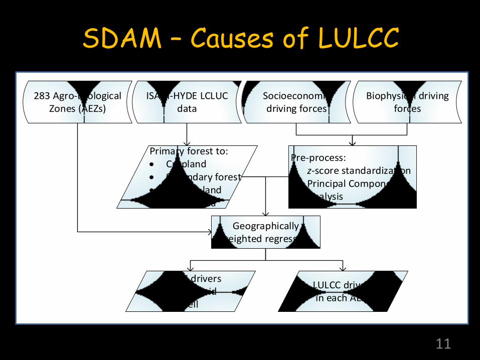
SDAM – Causes of LULCC

ISAM-HYDE LCLUC data

LULCC drivers of each grid

cell

Socioeconomic driving forces

Biophysical driving forces

LULCC drivers in each AEZs

Primary forest to: Cropland Secondary forest Pasture land Urban area

Pre-process: z-score standardization Principal Component

Analysis

283 Agro-Ecological Zones (AEZs)

Geographically weighted regression

11

ISAM – HYDE LCLUC Data

12

Estimated Forest Area (1990s) - Comparison with Previous Studies (Unit million km2)

Regions

Hurtt et

al.

(2006)

LUH2

(Hurtt et al.

2017)

ISAM-HYDE

(Consistent with IGBP

Classification)

Test Case

FAO2 ISAM-HYDE (UMD

Classification)

North America 9.3 8.1 5.8-6.0 5.1 4.1-4.5

Latin America 9.0 8.2 7.4-8.3 10.2 9.8-10.1

Europe 1.6 1.3 1.3-1.4 1.7 1.5

North Africa and

Middle East <0.1 <0.1 <0.1 0.1 0.4

Tropical Africa 4.4 3.4 2.8-3.15 6.9 7.0-9.8

Former USSR 9.7 8.8 5.9-6.0 8.1 6.3- 6.5

China 2.5 2.1 1.2-1.35 1.7 1.8- 2.0

South & South East

Asia 3.3 3.2 3.1-3.2 3.6 3.3- 3.4

Pacific Developed

Region 1.1 1.0 1.1 2.2 2.4- 3.7

World 40.9 36.2 29.0-30.1 39.6 37.2-41.3

Driver Data – Biophysical and Socioeconomic Data sets

Category Data Variable Description/Units Spatial Characteristics Period of Availability Source

Terrain (1) Elevation, Slope and Inclination Combined

Categorical Data classified into 9 gradient

classes

5 minutes^ (lat/lon)

Constant with time

FAO/IIASA, 2010. Global Agro-ecological Zones

(GAEZ v3.0). FAO, Rome, Italy and IIASA,

Laxenburg, Austria. http://www.fao.org/nr/

gaez/en/

Soil characters (5)

Soil fertility Categorical Data

classified into 7 gradient classes of land suitability

for agriculture

Soil drainage Chemical composition

Soil depth

Soil texture

Temperature (6) Temperature (Ta)

oC 0.5 degrees 1901-2009

Climatic Research Unit (CRU) TS 3.1 (updated

estimates based on Mitchell and Jones, 2005)

Daily Average Maximum Temperature (Tmax)

(lat/lon) (monthly)

Seasonal PET (4) Potential

Evapotranspiration Millimeters

Precipitation (7) Precipitation CRU TS 3.10.01#

Seasonal PDSI (4) Palmer Drought Severity

Index (PDSI) No units 2.5 degrees@ 1870-2010 Dai et al. (2011a,b)

Seasonal THI (4) Temperature humidity

index (THI) oC

Socioeconomic Factors (7)

Urban/built-up land % of grid-cell area 5 minutes^ 10,000 BC – 2005 AD Goldewijk et al. (2010) Urban Population

Inhabitants/km2 (lat/lon) (decadal)%

Rural Population

Gross Domestic Product (GDP) per capita

Constant 1990 international (Geary-

Khamis) dollars/person National level

1 AD-2010 Bolt and Van Zanden

(2013)

(annually between 1800-2010)$

(The Maddison Project - http://www.ggdc.net/m

addison/maddison-project/home.htm)

Market Accessibility No units 1 km^

~2005 Verburg et al. (2011) (lat/lon) 13

LULCC Activities Studied

• Following activities – Primary forest to cropland

– Primary forest to secondary forest

– Primary forest to pasture land

– Primary forest to urban area

• Over the time period 1900-2005

14

Base map (1900)

1920

2005

Reference map -HYDE Modeled map - SDAM

1960

SDAM downscaling results - Cropland

15

Unit: %

1920

2005

1960

Base map (1900)

SDAM downscaling results: Pastureland

16

Reference map -HYDE Modeled map - SDAM

Unit: %

Results: Primary forest to cropland

Overall dominant driver Dominant driver in each grid Dominant driver by AEZ

Market influence index: • downscaled GDP per capita

by market accessibility

Change in rural population density

Change in rural population density

Values refer to how many standard deviations the LULCC areas will change, per standard deviation increase in the drivers

Change in urban population density

1900~1919

1940~1959

1980~2005 Terrain

Soil

Temp

erature

Precip

itation

THI

PD

SI

PET

Market In

fluen

ce Ind

ex

Urb

an area

Urb

an p

op

ulatio

n

Ru

ral po

pu

lation

2 0

-2 2 0

-2 2

0 -2

17

Change in rural population density

Change in rural population density

Change in urban population density

1900~1919

1940~1959

1980~2005 2

0 -2

2 0 -2

2 0

-2

Results: Primary forest to secondary forest

1900~1919

1940~1959

1980~2005

Rural population density

Mean fall precipitation

Standard deviation of annual precipitation

Terrain

Soil

Temp

erature

Precip

itation

THI

PD

SI

PET

Market In

fluen

ce Ind

ex

Urb

an area

Urb

an p

op

ulatio

n

Ru

ral po

pu

lation

2 0

-2 2 0 -2 2

0 -2

18

Overall dominant driver Dominant driver in each grid Dominant driver by AEZ

Take Home Message • Spatial land use modeling and other tools

necessary to bridge scales between human and ESMs

• Both biophysical and socioeconomic drivers will strongly modulate climate change implications for agriculture, forest and other land use

• Understanding the drivers and dynamics of LULCC over the historical time can help to improve IAM-based projections of LULCC on a longer time scales

19

Near Term Research Plan

• Analyze the drivers of more LCLUC types

• Synthesize case studies at different scales to evaluate the LCLUC drivers

• Implement SDAM into GCAM

20

The End

21

SDAM

• Two objectives – downscale agricultural, forest and other land

use and changes from large world regions to the grid cell level

– determine the causes of these changes • The SDAM estimated land use changes

within each grid cell are driven by nonlinear interactions between – socioeconomic conditions (e.g. population,

technology, and economy), – biophysical characteristics of the land (e.g.

soil, topography, and climate), and – land use history

22

Geographically Weighted Regression (GWR)

• GWR constructs a distinct relationship between each LULCC grid cell and driving variables by incorporating grid cells falling within a certain bandwidth of the target pixel

23

β0 + β1 × Biophysical + β2 × Socioeconomic = LCLUC

β0 + β1 Population + β2 Temperature = LCLUC

β0 + β1 Population + β2 Temperature = LCLUCβ0 + β1 × Biophysical + β2 × Socioeconomic = LCLUC

Intercept

LULCC Activities Studied

• Following activities – Primary forest to cropland

– Primary forest to secondary forest

– Primary forest to pasture land

– Primary forest to urban area

• Over the time period 1900-2005

24