investigation of particle measurement in different
TRANSCRIPT

Graduate Theses, Dissertations, and Problem Reports
2020
Investigation of Particle Measurement in Different Dilution Ratios Investigation of Particle Measurement in Different Dilution Ratios
with Gasoline Direct Injection and Port Fuel Injection with Gasoline Direct Injection and Port Fuel Injection
John Adam Phillips West Virginia University, [email protected]
Follow this and additional works at: https://researchrepository.wvu.edu/etd
Part of the Automotive Engineering Commons
Recommended Citation Recommended Citation Phillips, John Adam, "Investigation of Particle Measurement in Different Dilution Ratios with Gasoline Direct Injection and Port Fuel Injection" (2020). Graduate Theses, Dissertations, and Problem Reports. 7815. https://researchrepository.wvu.edu/etd/7815
This Thesis is protected by copyright and/or related rights. It has been brought to you by the The Research Repository @ WVU with permission from the rights-holder(s). You are free to use this Thesis in any way that is permitted by the copyright and related rights legislation that applies to your use. For other uses you must obtain permission from the rights-holder(s) directly, unless additional rights are indicated by a Creative Commons license in the record and/ or on the work itself. This Thesis has been accepted for inclusion in WVU Graduate Theses, Dissertations, and Problem Reports collection by an authorized administrator of The Research Repository @ WVU. For more information, please contact [email protected].

INVESTIGATION OF PARTICLE MEASUREMENT IN
DIFFERENT DILUTION RATIOS WITH A GASOLINE DIRECT
INJECTION AND PORT FUEL INJECTION VEHICLE
John Adam Phillips
Thesis Submitted to the
Benjamin M. Statler College of Engineering and Mineral Resources at
West Virginia University
In partial fulfillment of the requirements for the degree of
Master of Science
in
Mechanical Engineering
Gregory Thompson, Ph. D., Chair
Arvind Thiruvengadam, Ph. D.
Derek Johnson, Ph. D.
Department of Mechanical and Aerospace Engineering
West Virginia University
Morgantown, West Virginia
2020
Keywords: Gasoline Direct Injection, Particle Measurement, Port Fuel Injection
Copyright 2020 John Adam Phillips

ABSTRACT
Investigation of Particle Measurement in Different Dilution Ratios
with a Gasoline Direct Injection and Port Fuel Injection Vehicle
John Adam Phillips
Ambient air quality has been a concern in the United States since the mid-1900’s, forcing
legislations like the Air Pollution Control Act and Clean Air Act necessary to bring focus on
air pollution and quality. The Environmental Protection Agency (EPA) continues to update the
requirements for more efficient vehicles and emissions sampling methods. Today the EPA has
implemented regulations on modern spark ignited engines without any major focus on the type
of injection technologies being used. While particle matter (PM) is a requirement to measure
for a vehicle certification, more research should focus on the particle number (PN)
measurements that are required for vehicle certification in the European Union. This study
explores the results of an experimental setup that measures particle data within multiple
simultaneous dilution ratio sampling environments. In addition to different dilution ratios, two
types of injection strategies were examined and included gasoline direct injected (GDI) and
port fuel injected (PFI). The emphasis of the study was the comparison of real time particle
number and mass concentration to highlight injection technologies effect on particles.
Furthermore, this research analyzed and compared the results in separate dilutions
environments to evaluate sampling from a high dilution ratio and determine whether this was
an acceptable sampling method. As engine technology, such as GDI, becomes the prominent
method of injection and PFI continues to be utilized, methods of soot measurement should be
improved to measure near 0.01 mg/m3. The PN measurements should be considered in addition
to current PM regulation with PN concentrations measured above 1x107 cm-3 during transient
test conditions.

iii
ACKNOWLEDGEMENTS
I often felt the more I prepared and conducted my research, I had created more work for myself
than when I initially started. With that being said, there are plenty of people that came along the
way to help whether it was at work or not. I would like to thank Dr. Gregory Thompson for helping
me to the completion of my research and for the initially opportunity to work for CAFEE years
ago as an undergrad. I would also like to thank my committee members Dr. Arvind Thiruvengadam
and Dr. Derek Johnson for their help during this process and guidance along my journey with
CAFEE. I would like to thank my dad Jack Phillips, my mother Pam Morgan, my step-mom Mandy
Phillips, my brother Ben Phillips, and my cousins Mikie and Travis Terry, my friends Dan and
Karen Skinner for all the support during my time as a masters student. I would like to thank my
close friends/co-workers Allen Duffy and Andrew Melcher as they both helped me in their own
way tremendously during my time as a graduate student and I cannot thank them enough for it. I
would also like to thank the staff of CAFEE: Dan Carder, Robert Cochran, Aaron Barnett, Ryan
Barnett, Stephen Cummings, Marc Besch, and Aaron Leasor. With a special thanks to Jason
England, Branson Tasker, Dylan Conelly, Matt Cummings, Sydnie Spencer, Marc Besch, Josh
Matheny, Phil Korpeck, Saroj Pradhan, and Ross Ryskamp.

iv
Table of Contents
ABSTRACT ................................................................................................................................................. ii
ACKNOWLEDGEMENTS ...................................................................................................................... iii
1. Introduction ......................................................................................................................................... 1
2. Objective/Scope ................................................................................................................................... 4
3. Literature Review ............................................................................................................................... 5
1. Health Effects....................................................................................................................... 5
2. Particle Matter ...................................................................................................................... 9
3. Gasoline Direct Injection ................................................................................................... 12
4. Relevant Research .............................................................................................................. 12
4. PM and Dilution Ratio Reduction ................................................................................................... 16
5. Methods and Materials / Experimental Set Up .............................................................................. 19
1. Dilution Ratios ................................................................................................................... 19
2. Test Plan............................................................................................................................. 29
3. Measurement and Testing Equipment ............................................................................... 32
4. Test Vehicles ...................................................................................................................... 32
5. 1065 Compliance ............................................................................................................... 35
6. Results ................................................................................................................................................ 36
1. PN Measurement ................................................................................................................ 38
2. MSS Measurement ............................................................................................................. 49
3. PM Collection .................................................................................................................... 58
7. Conclusions ........................................................................................................................................ 59
8. Recommendations ............................................................................................................................. 60
9. Appendix ............................................................................................................................................ 61

v
10. References .................................................................................................................................... 101

vi
Table of Figures FIGURE 1: ILLUSTRATION OF WALL-GUIDED DIRECT INJECTION (A) AND SPRAY-GUIDED DIRECT INJECTION
(B) (GCC 2006). ................................................................................................................................... 3 FIGURE 2: RESULTS FROM (MCCAFFERY, ET AL. 2019) OF THE SOOT MASS (A) AND GRAVIMETRIC MASS
(B) FROM TEST VEHICLES OVER FOUR TEST ROUTES. ........................................................................... 8 FIGURE 3: RESULTS FROM (MCCAFFERY, ET AL. 2019) OF THE PARTICLE NUMBER EMISSIONS OVER THE
FOUR TEST ROUTES WITH GDI VEHICLES. ............................................................................................ 9 FIGURE 4: TYPICAL ENGINE EXHAUST PARTICLE SIZE DISTRIBUTION (BESCH 2016) VISUALIZING THE
CONCENTRATION AND MASS WEIGHT OF PARTICLES IN THE DIFFERENT MODES. ............................... 11 FIGURE 5: GASEOUS RESULTS FROM (KARAVALAKIS, ET AL. 2015)THC (A), NMHC (B), CO2 (C), AND
FUEL ECONOMY (D) FOR WG-DI AND SG-DI WITH SIX DIFFERENT FUELS OVER THE FTP AND UC
CYCLE. ................................................................................................................................................ 14 FIGURE 6: AVERAGE PARTICLE SIZE DISTRIBUTION FROM (KARAVALAKIS, ET AL. 2015), OF AN WG-DI
VEHICLE (A) AND AN SG-DI (B) FOR A FTP AND UC CYLE. SIX DIFFERENT FUELS WERE TESTED FOR
BOTH CYCLES. ..................................................................................................................................... 15 FIGURE 7: DR 1 REFERENCE IMAGE 1. ........................................................................................................ 20 FIGURE 8: DR 1 AND 2 REFRENCE IMAGE 2. ................................................................................................ 21 FIGURE 9: PROBE LOCATION FOR DR 1 CPC. ............................................................................................. 21 FIGURE 10: VISUAL OF THE DR 2 SAMPLE TUNNEL. ................................................................................... 22 FIGURE 11 EJECTOR DILUTOR FOR DR 3 ..................................................................................................... 23 FIGURE 12: VISUAL AND DESCRIPTION OF EJECTOR DILUTOR OPERATION (AIR-VAC 2011). ..................... 23 FIGURE 13: VISUAL OF THE TEST STAND THAT CONTAINS THE DR 3 SAMPLE TUNNEL. ............................. 24 FIGURE 14: INTRODUCTION OF THE DILUTION AIR INTO THE DR 2 SAMPLE. .............................................. 25 FIGURE 15: FLOW PATH OF DLMB DILUTED SAMPLE FROM THE CVS TUNNEL. ........................................ 26 FIGURE 16: VIEW OF THE INSIDE PM BOX A AND BOX B. .......................................................................... 28 FIGURE 17: VACUUM PUMP USED FOR TEST SYSTEM. ................................................................................. 29 FIGURE 18: TEST VEHICLE 1, 2013 HYUNDAI SANTA FE. ........................................................................... 33 FIGURE 19: 2014 HYUNDAI SANTA FE EMISSION CONTROL INFORMATION LABEL. .................................. 33 FIGURE 20: TEST VEHICLE 2, 2015 SUBARU LEGACY................................................................................. 34 FIGURE 21: 2015 SUBARU LEGACY EMISSION CONTROL INFORMATION LABEL. ....................................... 34 FIGURE 22: EMISSIONS STANDARD FOR EPA TIER 2 BIN 4 & 5. ................................................................. 34 FIGURE 23: PM FILTER SPECIFICATIONS PER 40 CFR PART 1065.170 (C)(2) (EVIROMENTAL PROTECTION
AGENCY 2014). ................................................................................................................................... 36 FIGURE 24: CPC CONCENTRATION AT DR 1 DURING CITY DRIVING CONDITIONS. ................................... 39 FIGURE 25: CPC CONCENTRATION AT DR 2 DURING CITY DRIVING CONDITIONS. ................................... 40 FIGURE 26: CPC CONCENTRATION AT DR 3 DURING CITY DRIVING CONDITIONS. ................................... 40 FIGURE 27: NORMALIZED VEHICLE SPEED AND CO2 AGAINST THE DR 1 CPC CONCENTRATION. ........... 41 FIGURE 28: EXPLODED VIEW OF NORMALIZED AXIS OF FIGURE 27. ........................................................... 42 FIGURE 29: CPC CONCENTRATION AT DR 1 DURING URBAN DRIVING CONDITIONS. ............................... 43 FIGURE 30: CPC CONCENTRATION AT DR 2 DURING URBAN DRIVING CONDITIONS. ............................... 44 FIGURE 31: CPC CONCENTRATION AT DR 3 DURING URBAN DRIVING CONDITIONS. ............................... 44 FIGURE 32: CPC CONCENTRATION AT DR 1 DURING HIGHWAY DRIVING CONDITIONS. ........................... 46 FIGURE 33: CPC CONCENTRATION AT DR 2 DURING HIGHWAY DRIVING CONDITIONS. ........................... 46 FIGURE 34: CPC CONCENTRATION AT DR 3 DURING HIGHWAY DRIVING CONDITIONS. ........................... 47 FIGURE 35: CPC CONCENTRATION AT DR 1 DURING LA92 DRIVING CYCLE. ........................................... 48 FIGURE 36: CPC CONCENTRATION AT DR 2 DURING LA92 DRIVING CYCLE. ........................................... 48 FIGURE 37: CPC CONCENTRATION AT DR 3 DURING LA92 DRIVING CYCLE. ........................................... 49 FIGURE 38: MSS CONCENTRATION AT DR 1 DURING CITY DRIVING CONDITIONS. .................................. 50 FIGURE 39: MSS CONCENTRATION AT DR 2 DURING CITY DRIVING CONDITIONS. .................................. 50

vii
FIGURE 40: MSS CONCENTRATION AT DR 3 DURING CITY DRIVING CONDITIONS. .................................. 51 FIGURE 41: MSS CONCENTRATION AT DR 1 DURING URBAN DRIVING CONDITIONS. ............................... 51 FIGURE 42: MSS CONCENTRATION AT DR 2 DURING URBAN DRIVING CONDITIONS. ............................... 52 FIGURE 43: MSS CONCENTRATION AT DR 3 DURING URBAN DRIVING CONDITIONS. ............................... 52 FIGURE 44: MSS CONCENTRATION AT DR 1 DURING HIGHWAY DRIVING CONDITIONS. .......................... 53 FIGURE 45: MSS CONCENTRATION AT DR 2 DURING HIGHWAY DRIVING CONDITIONS. .......................... 54 FIGURE 46: MSS CONCENTRATION AT DR 3 DURING HIGHWAY DRIVING CONDITIONS. .......................... 54 FIGURE 47: MSS CONCENTRATION AT DR 1 DURING THE FIRST HALF OF THE LA92 DRIVING CONDITIONS.
............................................................................................................................................................ 55 FIGURE 48: MSS CONCENTRATION AT DR 1 DURING THE SECOND HALF OF THE LA92 DRIVING
CONDITIONS. ...................................................................................................................................... 55 FIGURE 49: MSS CONCENTRATION AT DR 2 DURING THE LA92 DRIVING CONDITIONS. .......................... 56 FIGURE 50: MSS CONCENTRATION AT DR 2 DURING THE FIRST HALF OF THE LA92 DRIVING CONDITIONS.
............................................................................................................................................................ 56 FIGURE 51: MSS CONCENTRATION AT DR 2 DURING THE SECOND HALF OF THE LA92 DRIVING
CONDITIONS. ...................................................................................................................................... 57 FIGURE 52: MSS CONCENTRATION AT DR 3 DURING THE LA92 DRIVING CONDITIONS. .......................... 57 FIGURE 53: SOOT PER MILE DURING THE LA92 TRANSIENT CYCLE> ......................................................... 58 FIGURE 54: O'KEEFE CONTROLS CO. ORIFICE DATA SHEET FOR METAL ORIFICE AIR FLOW IN SCFM. .. 61 FIGURE 55: PM WEIGHTS FROM HYUNDAI SANTA FE TESTS. .................................................................... 62 FIGURE 56: PM WEIGHTS FROM SUBARU LEGACY TESTS 1 OF 2. .............................................................. 63 FIGURE 57: PM WEIGHTS FROM SUBARU LEGACY TESTS 2 OF 2. .............................................................. 63 FIGURE 58: GRAVIMETRIC MASS RESULTS FROM CITY CONDITIONS WITH THE HYUNDAI. ....................... 64 FIGURE 59: GRAVIMETRIC MASS RESULTS FROM CITY CONDITIONS WITH THE SUBARU. ......................... 64 FIGURE 60: GRAVIMETRIC MASS RESULTS FROM URBAN CONDITIONS WITH THE HYUNDAI. ................... 65 FIGURE 61: GRAVIMETRIC MASS RESULTS FROM URBAN CONDITIONS WITH THE SUBARU. ..................... 65 FIGURE 62: GRAVIMETRIC MASS RESULTS FROM HIGHWAY CONDITIONS WITH THE HYUNDAI. .............. 66 FIGURE 63: GRAVIMETRIC MASS RESULTS FROM HIGHWAY CONDITIONS WITH THE SUBARU. ................. 66 FIGURE 64: GRAVIMETRIC MASS RESULTS FROM LA92 DRIVE CYCLE WITH THE HYUNDAI. ..................... 67 FIGURE 65: GRAVIMETRIC MASS RESULTS FROM LA92 DRIVE CYCLE WITH THE SUBARU. ....................... 67 FIGURE 66: AERIAL VIEW EMPTY TEST CELL WITH MULTI-DILUTION SETUP INSTALLED. ....................... 68 FIGURE 67: SIDE VIEW EMPTY TEST CELL WITH MULTI-DILUTION SETUP INSTALLED #1. ....................... 68 FIGURE 68: SIDE VIEW EMPTY TEST CELL WITH MULTI-DILUTION SETUP INSTALLED #2. ....................... 69 FIGURE 69: OVERVIEW OF CONTROL ROOM FOR TEST CELL. .................................................................... 69 FIGURE 70: ZOOMED LEFT VIEW OF CONTROL ROOM FOR TEST CELL. .................................................... 70 FIGURE 71: ZOOMED RIGHT VIEW OF CONTROL ROOM FOR TEST CELL. ................................................... 70 FIGURE 72: GAS BOTTLE RACK CONTAINING SPAN GASES FOR ANALYZERS ON TEST STAND. ................ 71 FIGURE 73: UNCOVERED VIEW OF WALL-MOUNTED DAQ BOX WITH TEST CELL EDGETECH HUMIDITY
SENSOR. .............................................................................................................................................. 71 FIGURE 74: COVERED VIEW OF WALL-MOUNTED DAQ BOX WITH TEST CELL EDGETECH HUMIDITY
SENSOR. .............................................................................................................................................. 72 FIGURE 75: BOX B PM BOX WITH DOOR SHUT. .......................................................................................... 72 FIGURE 76: WIRING OF THE TEMPERATURE CONTROLLERS FOR PM BOX B. ............................................ 73 FIGURE 77: BOX B PM BOX WITH DOOR OPEN. .......................................................................................... 73 FIGURE 78: ZOOMED IN VIEW OF THE INTERNALS OF PM BOX B............................................................... 74 FIGURE 79: SIDE VIEW OF THE THIRD DILUTION TUNNEL, DR 3 ANALYZER RACK TEST STAND, AND PM
BOX A. ................................................................................................................................................ 75 FIGURE 80: ZOOMED IN VIEW OF THE INTERNALS OF PM BOX A. ............................................................. 76 FIGURE 81: CLOSER OF THE DR 3 DILUTION TUNNEL (MOST RIGHT TUNNEL). .......................................... 77 FIGURE 82: ZOOMED FRONT LEFT VIEW OF THE ANALYZER RACK TEST STAND. ..................................... 78 FIGURE 83: FRONT VIEW OF THE ANALYZER RACK TEST STAND. ............................................................. 79

viii
FIGURE 84: ZOOMED VIEW OF THE DR 3 EJECTOR DILUTOR AND MASS FLOW CONTROLLER. ................. 79 FIGURE 85: DR 3 AND RAW CO2 ANALYZERS WITH THE SWITCHBOARD TO ZERO/SPAN/SAMPLE ABOVE.
............................................................................................................................................................ 80 FIGURE 86: FID ANALYZER USED TO PERFORM PROPANE INJECTIONS FOR DR 3 DILUTION
CONFIRMATION. ................................................................................................................................. 80 FIGURE 87: ISOTROPIC VIEW WITHOUT COVER OF THE DAQ BOX MOUNTED ON THE ANALYZER RACK
TEST STAND........................................................................................................................................ 81 FIGURE 88: FRONT VIEW WITH COVER OF THE DAQ BOX MOUNTED ON THE ANALYZER RACK TEST
STAND. ................................................................................................................................................ 81 FIGURE 89: ICP-CON #2 IN DAQ BOX MOUNTED ON ANALYZER RACK TEST STAND. ............................. 82 FIGURE 90: ICP-CON #1 IN DAQ BOX MOUNTED ON ANALYZER RACK TEST STAND. ............................. 82 FIGURE 91: POWER SUPPLY FOR EQUIPMENT IN DAQ BOX ON ANALYZER RACK TEST STAND. .............. 83 FIGURE 92: STARTECH TO CONNECT CPC'S, MSS'S, AND MFC'S IN DAQ BOX ON ANALYZER RACK TEST
STAND. ................................................................................................................................................ 83 FIGURE 93: FRONT VIEW OF TEMPERATURE CONTROLLERS FOR EXPERIMENTAL SETUP (BOX #1). ......... 84 FIGURE 94: BACK VIEW OF TEMPERATURE CONTROLLERS FOR EXPERIMENTAL SETUP (BOX #1). .......... 84 FIGURE 95: UNCOVERED SIDE VIEW OF TEMPERATURE CONTROLLERS FOR EXPERIMENTAL SETUP (BOX
#1)....................................................................................................................................................... 85 FIGURE 96: FRONT VIEW OF TEMPERATURE CONTROLLERS FOR EXPERIMENTAL SETUP (BOX #2). ......... 86 FIGURE 97: UNCOVERED SIDE VIEW OF TEMPERATURE CONTROLLERS FOR EXPERIMENTAL SETUP (BOX
#2)....................................................................................................................................................... 86 FIGURE 98: DILUTION TUNNEL FOR DR 2 WITH THE DR 2 PM BOX (DLMB) IN THE BACK. ..................... 87 FIGURE 99: DILUTION TUNNEL FOR DR 2, TOP VIEW. ................................................................................ 88 FIGURE 100: HORIBA OBS-ONE USED TO SAMPLE ON DR 2 WITH SPAN/ZERO CAL GASSES ON BOTTLE
RACK. ................................................................................................................................................. 88 FIGURE 101: HORIBA OBS-ONE FRONT VIEW. .......................................................................................... 89 FIGURE 102: HORIBA OBS-ONE ZOOMED SIDE VIEW. .............................................................................. 90 FIGURE 103: HORIBA OBS-ONE SOFTWARE COMPUTER. .......................................................................... 91 FIGURE 104: OVERVIEW OF THE TEST CELL WITH THE HYUNDAI TEST VEHICLE. ..................................... 92 FIGURE 105: REAR VIEW OF THE TEST CELL WITH THE HYUNDAI TEST VEHICLE..................................... 92 FIGURE 106: SIDE REAR VIEW OF THE TEST CELL WITH THE HYUNDAI TEST VEHICLE. ........................... 93 FIGURE 107: FRONT TOP VIEW OF THE TEST CELL WITH THE HYUNDAI TEST VEHICLE. .......................... 93 FIGURE 108: IMAGE #1 OF ALL EQUIPMENT IN PLACE DURING THE HYUNDAI TESTING. ........................... 94 FIGURE 109: IMAGE #2 OF ALL EQUIPMENT IN PLACE DURING THE HYUNDAI TESTING. ........................... 95 FIGURE 110: IMAGE #3 OF ALL EQUIPMENT IN PLACE DURING THE HYUNDAI TESTING. ........................... 95 FIGURE 111: IMAGE #4 OF ALL EQUIPMENT IN PLACE DURING THE HYUNDAI TESTING. ........................... 96 FIGURE 112: IMAGE #1 OF THE TEST CELL DURING THE SUBARU TESTING. .............................................. 97 FIGURE 113: IMAGE #2 OF THE TEST CELL DURING THE SUBARU TESTING. .............................................. 98 FIGURE 114: IMAGE #3 OF THE TEST CELL DURING THE SUBARU TESTING. .............................................. 98 FIGURE 115: IMAGE #4 OF THE TEST CELL DURING THE SUBARU TESTING. .............................................. 99 FIGURE 116: IMAGE #5 OF THE TEST CELL DURING THE SUBARU TESTING. .............................................. 99 FIGURE 117: IMAGE #6 OF THE TEST CELL DURING THE SUBARU TESTING. ............................................ 100 FIGURE 118: IMAGE #7 OF THE TEST CELL DURING THE SUBARU TESTING. ............................................ 100
ix
List of Tables
TABLE 1: TEST VEHICLE SPECIFICATIONS (MCCAFFERY, ET AL. 2019). ....................................................... 6 TABLE 2: TEST PLAN OF EQUIPMENT AND DESIGNATED DILUTION RATIO THE VEHICLE 1 (2013 HYUNDAI
SANTA FE). ......................................................................................................................................... 31 TABLE 3: TEST PLAN OF EQUIPMENT AND DESIGNATED DILUTION RATIO THE VEHICLE 2 (2015 SUBARU
LEGACY). ............................................................................................................................................ 31 TABLE 4: OUTLINE OF TEST CYCLE NUMBERS WITH CORRESPONDING TESTING CONDITIONS AND TEST
VEHICLE. ............................................................................................................................................. 37 TABLE 5: EQUIPMENT TYPE, MEASURING LOCATION, AND MEASURING TRAITS. ........................................ 38
1
1. Introduction
Ambient air quality has been a concern in the US since the mid 1900’s and continues to be a
concern. The 1955 Air Pollution Control Act was the first federal legislation in the United States
to address air quality and the 1963 Clean Air Act was the first legislation to control air pollution
(Shouse and Lattanzio 2020). Across the world, other countries are becoming more conscience of
their role in air pollution and have passed ambient air regulations with goals to preserve local
environmental health and welfare and global aspects like the ozone layer or reduce ambient carbon
dioxide levels (EPA 2020, Shouse and Lattanzio 2020, Eviromental Protection Agency 2014,
ECE/TRANS/505/Rev.7/Add.48 2015). In the United States, the Environmental Protection
Agency (EPA) enforces the emissions regulations set in place. The primary local environmental
health criteria air pollutants that are regulated include carbon monoxide, lead, nitrogen dioxide,
ozone, particulate matter, and sulfur dioxide (Eviromental Protection Agency 2014).
Modern day internal combustion engines operating on the Otto cycle are restricted to the Tier 3
emissions levels set forth by the EPA. This emissions regulation was one of the last phases since
January 1, 2000 with the implementation of the Tier 1 emissions requirements. Recent regulations
have forced manufacturers to focus on improved efficiency and improved technologies to meet
Tier 3 requirements (Eviromental Protection Agency 2014). Many manufacturers are now
producing internal combustion engines with direct injection method of fuel injection for spark
ignited engines (EPA 2020). This method of fuel injection is similar to the injection process of a
compression ignition engine. Compression ignition relies on using the change in volume of the
trapped air to pressurize the air and fuel in the cylinder, causing the temperature to rapidly increase.
At the desired time, fuel is injected into the cylinder and the heat available within the trapped air
ignites the fuel-air mixture. Gasoline direct injection (GDI) uses a similar injection strategy by
injecting directly into the cylinder, allowing for more effective atomization of the fuel, and
achieving an improved mixing of the fuel compared to port fuel injection (PFI) strategies. The
GDI process still requires a spark plug to ignite the air/fuel mixture. Increasing the compression
ratio allows for a cylinder pressure which often leads to higher efficiency of the engine. Increasing
the engine efficiency will lead to a more effective use of energy available and should reduce the
emissions emitted (Heywood 1988, Awad, et al. 2020, Moon, et al. 2017).

2
Using GDI technology may provide an improved injection method to increase engine efficiency
but it also has downsides. When using GDI, particulate matter (PM) and particulate number (PN)
levels significantly increase when compared to the PFI technology (Zhao 2009, Ko et al. 2018).
Concerns over possible health risks of increased particulate levels could drive new regulations in
the United States similar to Euro VI regulations on PN level in the European Union. Euro VI
regulation requires that gasoline engines operating with direct injection produce a maximum of
0.005 g/km of PM and 6.0 x 10¹¹ #/km of PN (Besch 2016, ECE/TRANS/505/Rev.7/Add.48 2015).
Direct injection has various forms but all with the same purpose: to inject fuel directly into the
combustion chamber near the crankshafts top dead center (TDC) at a high pressure. Spray-guided
and wall-guided are the most common forms of direct injection and combined have been reported
to consist of more than 50% of the model year (MY) 2019 vehicles (Zhao 2009, EPA 2020). Figure
1 presents an overview of GDI injection methods with wall-guided denoted “A)” and spray-guided
“B)”.

3
Figure 1: Illustration of wall-guided direct injection (A) and spray-guided direct injection (B) (GCC 2006).
Reducing particle mass and concentration in GDI vehicles is completed using a gasoline particulate
filter (GPF). GPFs are comparable to the diesel particulate filters (DPF) used on diesel engines. A
GPF will usually have lower filtration efficiency because the GDI engine lacks soot accumulation
inside the GPF (Awad, et al. 2020, Saito, et al. 2011). Using a GPF with a three way catalyst
(TWC) can result in a filtration efficiency above 90% in some cases (Awad, et al. 2020). Using a
GPF may prevent potential negative health issues from inhaled particulates. However, PN
regulations may need to be enacted to further reduce particle emissions, and their impact, being
emitted from GDI vehicles. A review of the literature is provided as a basis to understand the health
concerns, engine operation, particle formation, and particle measurement.
Presently, regulations in the United States only requires gravimetric-based PM measurements
utilizing a chassis dynamometer system to quantify the particulate emissions emitted from light
duty passenger vehicles. However, the PN may be equally important to human and environmental
4
health and should be considered. In the vehicle certification, a chassis dynamometer is used to
prescribe a load versus speed (time) that the vehicle must follow. Different speed versus time
profiles are used to mimic different driving conditions to evaluate the vehicle’s engine and
aftertreatment system. The subsequent emissions generated in the engine and aftertreatment are
then ducted to a dilution tunnel where the raw exhaust is mixed with conditioned air to form a
dilute mixture. This dilute mixture is then sampled for the regulated gaseous species and particulate
matter for gravimetric analysis. The dilution tunnel system can also be utilized for PN
measurement. However, the dilution ratio, along with other conditions, affects the way in which
the particulates form and hence will affect the PN. There is a need to understand the effects of the
dilution process on PN.
2. Objective/Scope
The overall objective of this work is to compare the particulate mass and concentration from a
single GDI spray-guided engine to a PFI configuration engine. To meet this objective, the two
vehicles were evaluated over three different steady state test cycle conditions and a LA92 transient
cycle on a chassis dynamometer and emissions collection system. These cycles simulated a city
route with the vehicle speed maintained at approximately 25 mph, an urban route with the speed
maintained at 45 mph, and a highway route with the speed maintained at 65 mph. During these
cycles, the carbon dioxide (CO2) was measured in the emissions collection to monitor the dilution
ratio. The focus was on particle emissions taken with AVL MicroSoot Sensors, TSI CPCs, and
gravimetric particle mass. These tests were conducted on a chassis dynamometer with three
separate dilution ratios. Dilution ratio 1 (DR 1) was measured from the constant volume sampling
(CVS) tunnel with a ratio of 20:1, dilution ratio 2 (DR 2) was sampled with a dilution ratio of
approximately 40:1, and dilution ratio 3 (DR 3) was sampled with a dilution ratio of approximately
80:1. These dilution ratios were all sampled simultaneously during a test cycle. By capturing these
results, a comparison between the two separate methods of injection and the effects of a
measurement environment on particle concentration were revealed.

5
3. Literature Review
1. Health Effects
A primary motivation for emissions regulations is the health of humans and the surrounding
environment. While the research discussed herein does not make any conclusion on the effects of
light duty GDI internal combustion engine emissions on the health of individuals or ambient air
quality, it is important to discuss the risk associated with the byproducts of an internal combustion
engine using GDI technology and especially the particulates produced. For human health, the
number of particles deposited on the lungs is dependent on the concentration of particles and their
size. Different particle sizes are capable of reaching different areas of the lungs. Particles smaller
than 5μm in diameter can reach the alveoli in a person’s lungs while particles above 5μm are only
capable of traveling to the proximal airways and are removed by the mucociliary clearance
(Sydbom, et al. 2001). Due to the decreased time period of fuel atomization and fuel impingement,
GDI engines are capable of producing up to twice the particle mass of a typical port fuel injection
(PFI) engine (Raza, et al. 2018). In the United States, the Tier 3 emissions standard is the present
regulation on light duty vehicles. This regulation holds no restriction on the particle number
concentration of light duty vehicles but only particle mass per unit distance traveled (Eviromental
Protection Agency 2014). In European regulation, a particle number concentration and mass are
imposed (ECE/TRANS/505/Rev.7/Add.48 2015). While meeting the requirement for particle
mass, it is possible that many of the nanoparticles can pass through the exhaust system and enter
the surrounding environment. As later explained in the section “Particle Matter,” nanoparticles are
low density particles. This allows large concentrations to be collected whilst only colleting a small
amount of mass (Besch 2016, Kittelson 1998). By restricting the particle number concentration
along with particle mass, the particle concentration must be reduced. PM emissions created from
gasoline spark ignited engines can be linked to lube oils and contribute nearly 25% of the overall
PM measurements (Raza, et al. 2018). Using a GPF can reduce the particle number concentration,
particle mass, and black carbon emissions. Studies have shown that a use of a catalyzed GPF can
improve the conversion efficiency of CO and NOx emissions (McCaffery, et al. 2019). McCaffery,
et al. 2019 conducted a study with three different GDI vehicles (two wall-guided and one spray-
guided) equipped with the original equipment manufacturer three-way catalyst (OEM TWC) used

6
to reduce the emissions for the Federal Tier 3 emissions standards. The technical specifications of
the test vehicles are provided in Table 1. The test routes performed are described later in the text.
Table 1: Test vehicle specifications (McCaffery, et al. 2019).
The OEM TWC was replaced with a GPF catalyst on GDI 1 and GDI 2 from Table 1 and the tests
repeated. The test was performed on road which required the use of portable emissions
measurement systems (PEMS). While gaseous species were measured, the focus of the current
section is health effects, and this study was used to provide data to show the benefit of a GPF.
Solid particle number emissions were measured using AVL’s M.O.V.E. PN PEMS iS for the wall-
guided GDI vehicles and the spray-guided GDI vehicle was instrumented with the NTK NCEM.
PN PEMS units used a corona diffusion charger type measurement system. The AVL M.O.V.E.
PN PEMS iS measures solid PN in accordance to the Particle Measurement Programme (PMP)
protocol while the NTK NCEM does not, due to measuring solid and volatile particles <23nm
(McCaffery, et al. 2019). This may contribute to a higher reported particle mass and number
concentration when compared to the wall guided vehicles. The three vehicles performed triplicate
tests for each of the four routes around the city of Los Angeles and Southern California. The four
routes were intended to embody traits of rural, urban, and highway driving conditions with varying
altitude and ambient climatic conditions. Routes have been labeled as “Downtown LA,”
“Highway,” “Mt Baldy,” and “Downtown SD.” “Downtown LA” was a 16-mile route of primarily
urban driving conditions with an average speed of 15.7 mph. The “Highway” route was high speed
driving over 43 miles with an average speed of 48.3 mph. The third route, “Mt Baldy,” began near
sea level and traveled up to an elevation of 1524 meters and back down to near sea level. The
elevation change can be attributed to the route traveling up Mountain Baldy and involved steep
grades up and downhill. This route maintained an average speed of 25.1 mph over the 44.2 miles.
The fourth route started and ended in downtown San Diego near the harbor. This route was

7
considered to have high ambient temperatures and relative humidity while traveling 13.1 miles
through mostly urban and some highway driving conditions. The tests were performed in order
from route one to three and the fourth, “Downtown SD,” was performed separately. Each test
began after the vehicle and TWC were at operating temperature.
The results for the soot mass and gravimetric mass is presented in Figure 2. Vehicle GDI 1
experienced a reduction in PM emissions ranging from 12%-49% while the soot mass emissions
were reduced by 44%-66% with the GPF catalyst installed. The GDI 2 vehicle reported a 60%-
96% reduction in PM emissions and 93%-99% reduction of soot mass emissions when installed
with a GPF. These results showed higher GPF filtration efficiencies for urban test routes when
compared to that of the Highway test route. While GDI 2 had much higher filtration efficiencies,
this is likely due to the lower engine-out PM levels of GDI 1.

8
Figure 2: Results from (McCaffery, et al. 2019) of the Soot mass (a) and gravimetric mass (b) from test vehicles over four
test routes.
Results of the particle number concentrations are presented in Figure 3. These results are similar
to the soot and particle mass of Figure 2. The results show that the vehicles with the GPF developed
a lower PN concentration over the different test routes. During the Mt. Baldy route, there was a
large PN concentration with GDI 2 that the author contributed to the NTK NCEM diffusion charger
method to measure particle concentrations. The NCEM infers a particle size distribution and
assumes an average diameter for all particles. In the text of (McCaffery, et al. 2019), it is
“hypothesized” that during higher engine loading, “small volatile or solid particles” formed in the
exhaust that may have also been below the cutoff size of 23 nm from the equipment. This resulted

9
in particles that normally would not be measured to increase the particle concentration for GDI 2.
From this, it was determined that the GPF could potentially store semi-volatiles and later release
them under certain driving conditions (McCaffery, et al. 2019).
Figure 3: Results from (McCaffery, et al. 2019) of the particle number emissions over the four test routes with GDI vehicles.
Particle emissions are reduced in (McCaffery, et al. 2019), meaning measures could be taken to
prevent these particles from being emitted. While this study is not focused on measuring the effect
of different GDI engines on public health, it is important to understand why particle emissions
from GDI engines are important to measure and control.
2. Particle Matter
PM in light duty internal combustion engines can be broken into three common sources: fuel
composition, lubrication oil, and rich combustion. Within these sources, PM can be categorized
into subgroups of solid, volatile, and semi-volatile. The subgroup is determined by whether the
chemical composition is organic or inorganic and its physical state (Awad, et al. 2020). Aerosols
are highly dependent on the environmental conditions the samples are collected from; for example,
residence time, local temperature of the aerosol, and dilution rates can change the properties of
aerosols and may cause them to be measured differently if the environmental conditions change.
Methods of measuring particles size depends heavily on the concentrations, particle size
10
distribution, and particle size measured (Besch 2016). PM emissions are formed as a product of
fuel combustion in the engine or by nucleation and condensation in the exhaust when cooled or
diluted during measurement (Awad, et al. 2020). From the particle distribution, the mode of the
particle by the size can be inferred. The three modes of a particle are nucleation mode,
accumulation mode, and coarse mode (Besch 2016). Nucleation mode is a range of particles
characterized for their size in the range of 3-30 nm. The lower limit of 3 nm has been limited due
to the lower detection limit of the equipment used at the time. Most particles in nucleation mode
are formed from cooling and/or diluting of volatile and semi-volatile organic compounds
(VOC/SVOC) from the engine exhaust. The VOC/SVOC are mainly made up of hydrocarbons
and sulfur compounds but will contain some ash and elemental carbon. While in a typical diesel
exhaust particle distribution, particles in nucleation mode will contain the most concentration of
particles (>90%), the mass of these particle size is relatively low (<20%). Sampling particles in
nucleation mode is the most challenging because of their sensitivity to the environment and
collection methods. Conditions including sample temperature, relative humidity, dilution rates,
and dilution ratios affect volatiles. The volatility of a particle can be defined by its evaporation
temperature. Solid particles (non-volatile) must have an evaporation temperature above 350 ⁰C.
Semi-volatile particles have an evaporation temperature of 100 ⁰C to 350 ⁰C, while volatile
particles must completely evaporate below 100 ⁰C (Besch 2016, Kittelson 1998). Accumulation
mode is defined by particles that are between 30-500 nm in diameter. While these particles are
higher in particle mass, they do not account for much of the concentration. These particles are not
significantly affected by dilution and sampling such as the particles in nucleation mode range.
Particles in the accumulation mode may still be impacted by particles re-volatilizing. These
particles are easily removed with particulate filters (Besch 2016). Particles in coarse mode are
characterized as those with a diameter of 500nm or greater. These particles account for 5-20% of
the total particle mass. Although these types of particles are measured during an engine or vehicle
test, they are usually found to be deposits from cylinder walls or exhaust piping/systems (Besch
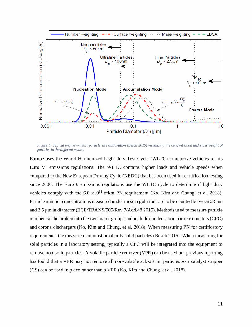
2016). These particles are of less interest for the purpose of this study. Figure 4 illustrates the
different modes of a particle and how their concentrations and mass compared to other modes.
11
Figure 4: Typical engine exhaust particle size distribution (Besch 2016) visualizing the concentration and mass weight of
particles in the different modes.
Europe uses the World Harmonized Light-duty Test Cycle (WLTC) to approve vehicles for its
Euro VI emissions regulations. The WLTC contains higher loads and vehicle speeds when
compared to the New European Driving Cycle (NEDC) that has been used for certification testing
since 2000. The Euro 6 emissions regulations use the WLTC cycle to determine if light duty
vehicles comply with the 6.0 x10¹¹ #/km PN requirement (Ko, Kim and Chung, et al. 2018).
Particle number concentrations measured under these regulations are to be counted between 23 nm
and 2.5 μm in diameter (ECE/TRANS/505/Rev.7/Add.48 2015). Methods used to measure particle
number can be broken into the two major groups and include condensation particle counters (CPC)
and corona dischargers (Ko, Kim and Chung, et al. 2018). When measuring PN for certificatory
requirements, the measurement must be of only solid particles (Besch 2016). When measuring for
solid particles in a laboratory setting, typically a CPC will be integrated into the equipment to
remove non-solid particles. A volatile particle remover (VPR) can be used but previous reporting
has found that a VPR may not remove all non-volatile sub-23 nm particles so a catalyst stripper
(CS) can be used in place rather than a VPR (Ko, Kim and Chung, et al. 2018).

12
3. Gasoline Direct Injection
In light duty gasoline fueled internal combustion engines, GDI has seen increased implementation
over the last 15 years. For example, model year 2008 vehicles had less than 3% GDI technologies
while model year 2019 projected 50% of the vehicles were GDI (EPA 2020). The reason modern
vehicles have been converting from PFI to GDI may be because the increased efficiency and
fueling control results in lower CO2 emissions (Karavalakis, et al. 2015). Within GDI technology,
there are two main methods of injection. Wall-guided DI (WG-DI) is a more common option for
GDI engines, having an injector mounted on the side and spraying toward a contoured piston that
projects the atomized fuel upward in the direction of the spark plug. While WG-DI engines may
be more common, they experience higher levels of PM and total hydrocarbons (THC). During the
combustion process, some of the fuel may contact the cylinder walls. If the fuel is quenched during
mixing in the chamber, incomplete combustion occurs locally and soot is formed, along with other
semi-volatiles (non-solid particles). THC is formed due to the incomplete evaporation and mixing
with air and absorption and desorption of the fuel trapped in the piston crevices and dissolved into
the lubrication oil. Spray guided DI (SG-DI) is an alternative method of injecting but less common
in the US because the lean fueling strategy would require an emissions control strategy for oxides
of nitrogen (NOx) (Karavalakis, et al. 2015).
4. Relevant Research
In the study performed by Karavalakis et al, both methods of injections in GDI engines were
evaluated with different blends of ethanol and iso-butanol. The different fuels included a E10 (10%
ethanol and 90% gasoline) for reference, an E15 ethanol blend, an E20 ethanol blend, and a
gasoline, iso-butanol blend. The gasoline iso-butanol blend was combined at 16%, 24%, and 32%
butanol which were comparable to E10, E15, and E20 ethanol fuels, respectively. Oxygen and fuel
volatility properties were matched, and the Reid vapor pressure (RVP) was retained within 6.4-
7.2psi. The test vehicles were both 2012 model year passenger cars with TWC. One vehicle being
a WG-DI with a 2.0 L engine and the other being SG-DI with 3.5 L engine. Each vehicle was
tested over three repeat Federal Test Procedure (FTP) cycles and three Unified Cycles (UC) with
each of the six fuels. Each vehicle completed all six tests with a single fuel type before multiple
drain and fill procedures were conducted to prepare for a new fuel. Gaseous test measurements
included THC, CO, NOx, NMHC, and CO2. DNPH cartridges were used for carbonyl analysis,

13
carbotrap adsorption tubes for volatile organic compounds (VOC), and an Agilent 6890 GC with
an FID maintained at 300 ⁰C was used to measure the VOCs. Particle number measurement was
measured with a TSI 3776 ultrafine-CPC for particle concentration, TSI EEPS for size distribution,
and mass based measured was measured with a 47 mm Teflon® filter. A Code of Federal
Regulation (CFR) Title 40 Part 1065 compliant microbalance measured the PM mass in a
controlled clean chamber environment. In the review of this paper, the focus was a comparison of
the spray-guided and wall-guided injection technologies rather than the different fuels. The fuel
most relevant to this research was the E15 ethanol blend since it will be most comparable to the
fuel being used in this research. The THC emissions were 0.012 g/mile for the spray-guided (SG-
DI) and 0.095 g/mile for the wall-guided (WG-DI) for the FTP cycle for the E15 blend. The THC
emissions for the UC test cycle showed a similar 0.018 g/mile for the SG-DI vehicle and the WG-
DI vehicle had a reduction of THC emissions resulting in 0.008 g/mile. It should be noted that in
Figure 5, the graph representing the THC have different scales. The THC emissions were
represented by the high concentrations seen in the first few hundred seconds, during the cold-start
portion. It was reported that the hot-start portion of the test had near zero THC emissions due to
the light off temperature being below the temperature of the TWC. THC emissions may have an
increased effect due to fuel impingement, especially for spark ignited direct injection engines. It is
also assumed that as the engine operates past the cold-start condition and the cylinder surface
temperature increases, an improved environment for fuel vaporization and pool fires occurs,
resulting in lower THC emissions (Karavalakis, et al. 2015). The CO2 emissions for the FTP cycle
showed 350 g/mile for the SG-DI and 250 g/mile for the WG-DI. The masses of the vehicles may
cause deviation due to the SG-DI vehicle using a 3.5 L engine compares to the 2.0 L WG-DI
engine. Whereas the CO2 emissions for the UC cycle reveal the SG-DI to have 350 g/mile and 280
g/mile for the WG-DI. The fuel economy results for the SG-DI for the FTP and the UC cycles
were 24 miles/gallon. For the WG-DI the fuel economy for the FTP was 34 miles/gallon while the
UC cycle implies the fuel economy was 30 miles/gallon. The results of these different vehicles
indicate that the SG-DI vehicle sees little to no change between the FTP and the UC cycle while
the WG-DI vehicles showed an increase of 20% in CO2 emissions and, subsequently, a 25%
decrease in fuel economy. The THC emissions from the UC cycle indicate a 40% decline when
compared to the FTP cycle.

14
Figure 5: Gaseous Results from (Karavalakis, et al. 2015)THC (a), NMHC (b), CO2 (c), and Fuel Economy (d) for WG-DI
and SG-DI with six different fuels over the FTP and UC cycle.
Figure 6 presents the particle size distribution from the study. The top portion of the figure
represents the WG-DI vehicle while the lower portion shows SG-DI particle size distribution. The
blue lines represent the E15 fuel which is most comparable to the fuel used in this research
discussed later and is the only particle distribution reviewed. The distributions are similar from
cycle to cycle but when comparing the direct injection methods, the SG-DI concentration shows a
decrease of approximately 1.0x105 cm-3 to the concentration of the WG-DI. Using the particle
distribution in Figure 6, the distribution shows most of the particles in accumulation mode with
the WG-DI engine. The WG-DI had a larger concentration of particles because of zones with rich
air fuel ratio (AFR). This rich localization comes from the injection charge cloud and is attributed
to the poor mixture preparation association with wall guided engine design. While it will not be

15
tested in the following research, it is important to note the decrease in average particle
concentrations when changing from ethanol fuel blends to iso-butanol blends. This highlights that
other options are available to further lower particle emissions that could aid hardware such as a
GPF to minimize particle concentration from tailpipe out emissions.
Figure 6: Average particle size distribution from (Karavalakis, et al. 2015), of an WG-DI vehicle (a) and an SG-DI (b) for a
FTP and UC cyle. Six different fuels were tested for both cycles.

16
4. PM and Dilution Ratio Reduction
In the United States, emissions testing falls under the CFR Title 40, Part 1065 umbrella. The
specific requirements for emissions testing are included in this and other sections. For gravimetric
PM, a 47 mm filter is required to trap a sample of the dilute exhaust for mass measurement. The
PM sampling requires a filter face velocity across a 38 mm diameter filter stain area to be 50
cm/sec or to target filter loading of 400 μg. Due to the high dilution ratios, 400 μg would require
a higher filter flow velocity and thus require the filter face velocity target of 50 cm/sec. The 50
cm/s filter face velocity can be translated into a flowrate of 2.3 SCFM using the dimensions for
the equipment and flow paths. The methods for two of the three PM sampling systems utilized
critical flow orifices to control the flowrate of the sample path.
With the dilute exhaust flow being predominately gas, there are multiple methods to measure and
record the flow rate of the sample streams. For example, critical flow orifices (CFO) will achieve
a constant velocity flow through them once a pressure ratio of the upstream and downstream
pressures has been achieved. A high vacuum system can be used to pull the sample though the
flow path and designed to provide an adequate pressure drop (∆P) across the CFO unless there is
a blockage or significant restriction, such as when the filters become overloaded with PM.
The CFO’s used were provided from O’Keefe Controls Company and using their data sheets
shown in Figure 54 in the Appendix, the orifice selected was Size Number 100. This size is
important in reference to the flow value at critical flow. In a choked flow setting, the flow of this
orifice is 59 SLPM. This value can be converted to 2.08 SCFM using standard conditions (70 °F
and 14.7psia). For a CFO to achieve critical flow, upstream (Pup-stream) and downstream (Pdown-
stream) pressure is compared to a pressure ratio. By dividing Pup-stream by Pdown-stream as shown below,
the absolute pressure ratio (Pratio) can be determined.
𝑃𝑟𝑎𝑡𝑖𝑜 =𝑃𝑢𝑝−𝑠𝑡𝑟𝑒𝑎𝑚
𝑃𝑑𝑜𝑤𝑛−𝑠𝑡𝑟𝑒𝑎𝑚
For the flow to be critical, the Pratio must be at least 0.528 at standard conditions (O'Keefe Controls
Co. 2011). Pressure ratios above this confirm a critical flow while ratios below do not. The
pressures being used for the calculation must be an absolute pressure as well.

17
The flowrate of the orifice will need correction factors for temperature (Tsample), pressure (P1),
viscosity (μ)and relative humidity (RHsample). Equations for RHsample and μ were found in a user
manual from Meriam for Laminar Flow Elements (Meriam n.d.).
𝑅𝐻𝑠𝑎𝑚𝑝𝑙𝑒 =𝜌𝑤𝑒𝑡
𝜌𝑑𝑟𝑦
The correction factor RHsample is calculated by dividing the density of wet air (ρwet) at the sample
condition by the density of dry air (ρdry) at the standard condition of the orifice.
𝜇𝑐𝑜𝑟𝑟 =𝜇𝑠𝑡𝑑
𝜇𝑚𝑒𝑎𝑠𝑢𝑟𝑒𝑑
The viscosity correction factor is the viscosity of air at standard temperature condition (μstd)
divided by the viscosity of the sampled air temperature condition (μmeasured).
Normally there is a K value for the geometry of the orifice, but this has already been factored into
the given flow rate from O’Keefe Controls Co. The temperature and pressure values of the sample
were recorded and the calculated real-time during the testing, while viscosity and humidity were
considered constant due to humidity measurement capabilities and viscosity being determined by
temperature which should remain constant with all heated sample paths. Humidity measurements
at sample locations were recorded but for reference only as the equipment was not calibrated nor
held a high measurement resolution. Heated lines were leak checked and temperature checked
before use. The equation below was used to calculate a corrected flow rate for two of the critical
flow orifices controlling sample flow for PM collection.
𝑄𝑎𝑐𝑡𝑢𝑎𝑙 = 𝑄𝑒𝑠𝑡 ∗529.67
(𝑇𝑠𝑎𝑚𝑝𝑙𝑒 + 459.67)∗
𝑃1
14.7∗ 𝑅𝐻𝑠𝑎𝑚𝑝𝑙𝑒 ∗ 𝜇𝑐𝑜𝑟𝑟
The first part of the equation is the estimated flow from O’Keefe Co. Next is the correction factor
for the temperature, the recorded temperature value (⁰F) is converted to Rankine and divided into
the temperature at the given standard condition, also in Rankine. Then the pressure is divided into
the atmospheric pressure given at standard conditions, in PSIA. As previously stated, relative
humidity and viscosity corrections were used by multiplying the correction factors by the estimated
flow.

18
Gravimetric PM is a mass measurement of the particles collected onto a filter during a test cycle.
The weight of the filter is recorded before the cycle starts and after. The calculation of the net filter
mass from a test cycle (Mcycle) is the difference between the from the Mpost (post-mass) and Mpre
(pre-mass).
𝑀𝑐𝑦𝑐𝑙𝑒 = 𝑀𝑝𝑜𝑠𝑡 − 𝑀𝑝𝑟𝑒
For comparison amongst other filters, the Mcycle will need to be equated to a normalized value to
allow for an even comparison. During the filter sampling, the flow across the filter is measured.
This flow measurement, with the time the sample valve is open during a test cycle allowed the
calculation of the volume sampled. From the data provided from a single test cycle, the number of
seconds the sample valve remained opened was summed (Tsampled). The volumetric flowrate is
taken and the mean flow rate from the moment the sample valve is opened, until it is closed, is
determined. This value (V̇avg) will represent the average flow from the beginning of filter sampling
until the end. Due to the high vacuum system and large flowrate required, there is a bypass valve
installed parallel to the sample valve. The bypass system flows the exhaust stream through the
sampling system, but around the filter housing, to maintain constant sampling conditions at the
beginning or end of test period and to maintain a consistent flow during a transition of sampling
paths. The Vsampled, is the total volume sampled across the filter and is calculated as such.
𝑉𝑠𝑎𝑚𝑝𝑙𝑒𝑑 = V̇avg ∗ Tsampled
Using Mcycle and Vsampled, the mass per volume sampled can be calculated to compare the particles
weights sampled at each dilution ratio.
𝑀𝑣𝑜𝑙 =𝑀𝑐𝑦𝑐𝑙𝑒
𝑉𝑠𝑎𝑚𝑝𝑙𝑒𝑑⁄
Mass per volume (Mvol) can be used to normalize the PM weights between cycles and dilution
ratios for basic comparisons.
Dilution ratio calculation is used to confirm the proper sample cycle to cycle. DR 1 exist in the
CVS tunnel of the test cell. Using the Horiba OBS-ONE, the exhaust flow rate (EFR) of the engine
compared to the CVS tunnel EFR, the dilution ratio can be calculated. DR 1 used CO2, along with
DR 2 and 3, to classify their dilution ratio. The methods for both are similar but with different
19
sources. For the exhaust flow, the recorded data for the CVS tunnel (Exhcvs) and Horiba OBS-ONE
(Exhobs) was time aligned and an average of the flows taken from the entire cycle time. This can
be seen from the equation below.
𝐷𝑖𝑙𝐷𝑅 1 =𝐸𝑥ℎ𝑐𝑣𝑠
𝐸𝑥ℎ𝑜𝑏𝑠
When using CO2, the process is similar. The CO2 traces were time aligned and an average of the
concentrations taken for the duration of the cycle. The average of the lower diluted system (i.e.
20:1<40:1) was divided by higher diluted system to yield a relative dilution ratio of the two
systems. Until the ratio is multiplied by the dilution ratio of the system it samples from, it is not
the final dilution ratio.
𝐷𝑖𝑙𝐷𝑅 𝑋 =𝐶𝑂2𝑐𝑜𝑛𝑐. 1
𝐶𝑂2𝑐𝑜𝑛𝑐. 2
Where CO2 conc. 1 is a lower dilution ratio system than CO2 conc. 2. The system used to conduct this
research used three dilution systems. If the first dilution ratio (CO2 conc. 1) is divided by the last
dilution ratio (CO2 conc. 3), the result would be Dilfinal.
5. Methods and Materials / Experimental Set Up
Equations used for the PM boxes with CFOs will be presented in the following section along with
the various equipment. All analyzers, pressure transducers, thermocouples, heated lines, and other
test critical equipment was verified and calibrated prior to testing to ensure data integrity.
1. Dilution Ratios
The sampling system consisted of three separate dilution ratios. These dilution ratios are labeled
as DR 1, DR 2, and DR 3. The DR 1 ratio is based on the CVS tunnel sampling system with a
Horiba critical flow orifice (CFO) sampling system to maintain constant flow. For this testing, the
flow rate of the tunnel was selected at 14.5 m3/min to achieve a dilution ratio of approximately
20:1. Figure 7 shows an overview of the test cell equipment. The Horiba cabinets in the background
house the sample bags that are filled during the test cycle. The Horiba cabinet to the right of them
is a MEXA 7000 that sampled all the gaseous species. At the right edge of Figure 7, the stainless-

20
steel pipe is the CVS tunnel. The back side of the CVS tunnel has a second flange that is symmetric
to the one shown by the blue arrow. This flange contains the probe for the DR 1 PM box (shown
above the blue MircoSoot Sensor (MSS) in Figure 8), and the heated sample line transferred the
sample to the Air-Vac ejector dilutor for DR 3. This flange is also where the MSS in Figure 8
measured. Further up the CVS tunnel by approximately 12” is a separate probe for the CPC. This
probe location can be seen circled in Figure 9.
Figure 7: DR 1 reference image 1.
DR 3
PM box
CVS Bagging
System
MEXA 7000
Gaseous Unit
CVS tunnel and
45⁰ sampling
flanges
DR 3 Sampling
Tunnel box
DR 3 MSS
box
DR 3
CPC
box
DAQ Box
Raw CO2
analyzer
DR 3 CO2
analyzer
DR 3 Temperature
Controllers

21
Figure 8: DR 1 and 2 refrence image 2.
Figure 9: Probe location for DR 1 CPC.
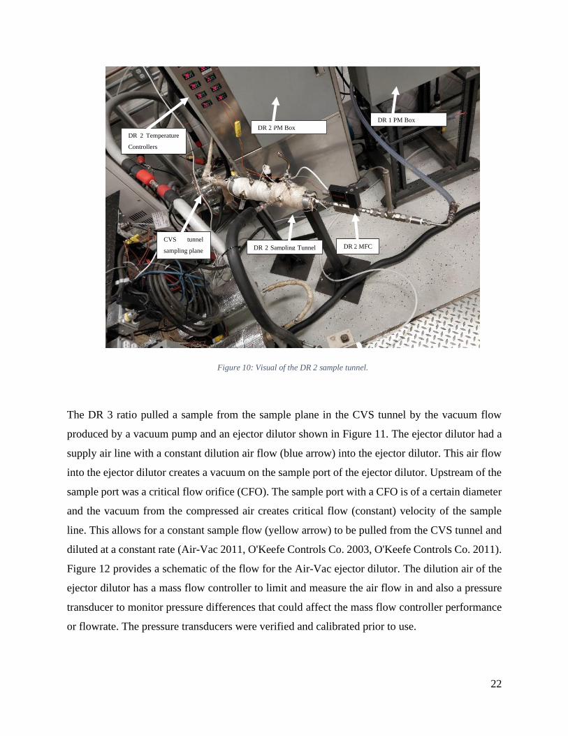
For DR 2, the sample traveled into the existing PM box on the CVS tunnel and be introduced to a
2:1 dilution, for an overall dilution ratio of 40:1. After passing through this dilution stage, the
sample traveled into a smaller, secondary tunnel that equipment measured from, shown in Figure
10. The filter loading took place in the grey box behind the small tunnel in Figure 10. The gaseous
measurement was taken with a Horiba OBS-ONE. This unit can be seen previously in Figure 8 to
the right.
DR 1 PM Box
OBS-ONE for
CO2 on DR 2
DR 2 PM Box
DR2 Sampling
Tunnel
DR 1 MSS DR 3 Sampling tunnel
Ejector Dilutor
DR 3 Dilution
Air MFC
DR 2 Sampling probe
Introduction of
dilution air for
DR 2
22
Figure 10: Visual of the DR 2 sample tunnel.
The DR 3 ratio pulled a sample from the sample plane in the CVS tunnel by the vacuum flow
produced by a vacuum pump and an ejector dilutor shown in Figure 11. The ejector dilutor had a
supply air line with a constant dilution air flow (blue arrow) into the ejector dilutor. This air flow
into the ejector dilutor creates a vacuum on the sample port of the ejector dilutor. Upstream of the
sample port was a critical flow orifice (CFO). The sample port with a CFO is of a certain diameter
and the vacuum from the compressed air creates critical flow (constant) velocity of the sample
line. This allows for a constant sample flow (yellow arrow) to be pulled from the CVS tunnel and
diluted at a constant rate (Air-Vac 2011, O'Keefe Controls Co. 2003, O'Keefe Controls Co. 2011).
Figure 12 provides a schematic of the flow for the Air-Vac ejector dilutor. The dilution air of the
ejector dilutor has a mass flow controller to limit and measure the air flow in and also a pressure
transducer to monitor pressure differences that could affect the mass flow controller performance
or flowrate. The pressure transducers were verified and calibrated prior to use.
DR 2 Sampling Tunnel
box
DR 2 PM Box
DR 1 PM Box
DR 2 MFC
DR 2 Temperature
Controllers
CVS tunnel
sampling plane

23
Figure 11 Ejector dilutor for DR 3
Figure 12: Visual and description of ejector dilutor operation (Air-Vac 2011).
This ejector dilutor flowed a sample into a separate secondary tunnel at a dilution ratio of 4:1, to
achieve a final dilution ratio of 80:1. The DR 3 sample passed through the first tunnel in the set of
three. This tunnel is shown in Figure 13 as having the grey heated sample line and tan colored box
DR 3 ejector dilutor
DR 3 dilution
air MFC
24
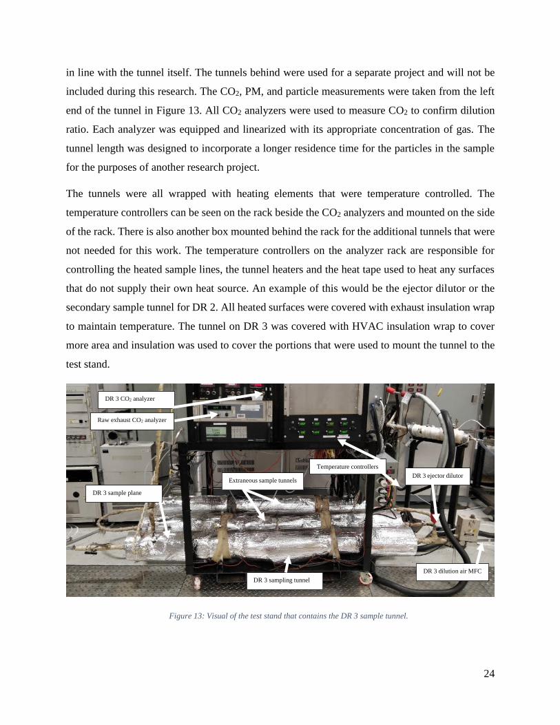
in line with the tunnel itself. The tunnels behind were used for a separate project and will not be
included during this research. The CO2, PM, and particle measurements were taken from the left
end of the tunnel in Figure 13. All CO2 analyzers were used to measure CO2 to confirm dilution
ratio. Each analyzer was equipped and linearized with its appropriate concentration of gas. The
tunnel length was designed to incorporate a longer residence time for the particles in the sample
for the purposes of another research project.
The tunnels were all wrapped with heating elements that were temperature controlled. The
temperature controllers can be seen on the rack beside the CO2 analyzers and mounted on the side
of the rack. There is also another box mounted behind the rack for the additional tunnels that were
not needed for this work. The temperature controllers on the analyzer rack are responsible for
controlling the heated sample lines, the tunnel heaters and the heat tape used to heat any surfaces
that do not supply their own heat source. An example of this would be the ejector dilutor or the
secondary sample tunnel for DR 2. All heated surfaces were covered with exhaust insulation wrap
to maintain temperature. The tunnel on DR 3 was covered with HVAC insulation wrap to cover
more area and insulation was used to cover the portions that were used to mount the tunnel to the
test stand.
Figure 13: Visual of the test stand that contains the DR 3 sample tunnel.
Temperature controllers
DR 3 sampling tunnel
Extraneous sample tunnels
DR 3 CO2 analyzer
Raw exhaust CO2 analyzer
DR 3 sample plane
DR 3 ejector dilutor
DR 3 dilution air MFC
25
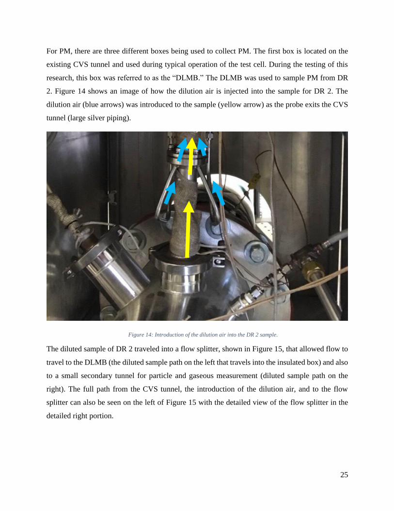
For PM, there are three different boxes being used to collect PM. The first box is located on the
existing CVS tunnel and used during typical operation of the test cell. During the testing of this
research, this box was referred to as the “DLMB.” The DLMB was used to sample PM from DR
2. Figure 14 shows an image of how the dilution air is injected into the sample for DR 2. The
dilution air (blue arrows) was introduced to the sample (yellow arrow) as the probe exits the CVS
tunnel (large silver piping).
Figure 14: Introduction of the dilution air into the DR 2 sample.
The diluted sample of DR 2 traveled into a flow splitter, shown in Figure 15, that allowed flow to
travel to the DLMB (the diluted sample path on the left that travels into the insulated box) and also
to a small secondary tunnel for particle and gaseous measurement (diluted sample path on the
right). The full path from the CVS tunnel, the introduction of the dilution air, and to the flow
splitter can also be seen on the left of Figure 15 with the detailed view of the flow splitter in the
detailed right portion.

26
Figure 15: Flow path of DLMB diluted sample from the CVS tunnel.
Once the sample for DR 2 travels into the DLMB, the sample will travel into an identical path as
the samples for DR 1 and DR 3, with the exception of flow measurement. For the DR2 DLMB PM
measurement, the flow was measured using a Alicat Scientific MCR-100SLPM-D mass flow
controller (MFC). The PM boxes for DR 1 and DR 2 were constructed prior to the beginning of
the project with all new tubing and custom flow splitters but used cyclones and valves from prior
projects. Figure 16 shows the components internal to PM Box A used to sample at DR 3 and PM
Box B used to sample at DR 1. The box was designed for use on a project parallel to the research
Sample path of DR 2
Detailed view

27
data collected and is the reason for the organization of the line routing. The blue lines indicate the
flow of the sample up to the exit of the filter holder. Once the sample is through the filter holder,
the lines change to green. The sample comes into the box, and immediately passes through the
cyclone to remove large particles via vortex separation. The flow travels out of the cyclone and
into a custom flow splitter designed to maintain isokinetic flow. The flow for this experiment only
travelled through the left filter holder. During the experiment, the right filter holder was removed,
and the exposed fittings were plugged. The sample passed over a single 47 mm TX40 filter, this is
where the sample line changes from blue to green. The sample passes through to the critical flow
orifice and the valve that opens/closes to introduce vacuum pressure to allow flow. In the sample
path, there is a small brass object underneath the filter holder in Figure 16 (circled in yellow). This
is the critical flow orifice (CFO) used to maintain a constant flow during the test cycles. The CFO
has been machined to a particular diameter and corrected for pressure, temperature, and humidity.
This equation of the flow can be seen in the PM and Dilution Ratio Reduction section. For the
corrections, the temperature and absolute pressure upstream of the CFO around the CFO were
recorded real time during the testing. Differential pressure was recorded across the CFO to confirm
an adequate pressure ratio between the upstream and downstream pressure to host critical flow.
The differential pressures were recorded using a Honeywell PPT010-1D-WW-2V-B. The absolute
pressure transducers were Omega PX176-02A5V models. These pressure transducers were
calibrated prior to installation and use in the research. The temperature measurement was measured
in the flow block with a J-type thermocouple. The vacuum source used was a Busch Mink MM
1104 BV vacuum pump, shown in Figure 17.

28
Figure 16: View of the inside PM Box A and Box B.

29
Figure 17: Vacuum pump used for test system.
For particle measurement, multiple MSS units and CPC units were used. Also, during the testing
of the Subaru Legacy, one MSS unit was not available and the second MSS unit was moved
between DR 2 and DR 3. This will all be explained in the text later for clarification. During the
testing of the Sant Fe, each dilution ratio had their own MSS, CPC, CO2 analyzer, and PM
measurement. The PM measurement details were explained in the previous section.
2. Test Plan
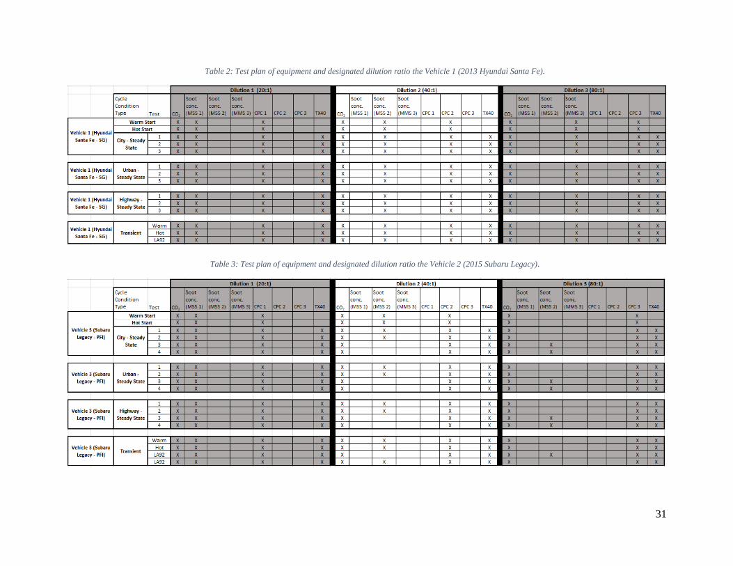
The test matrix is shown in Table 2 and Table 3. This overview of the tests shows there were three
different steady state conditions: City, Urban, and Highway. The City conditions was driven on
the chassis dynamometer at approximately 25mph, the Urban at 45mph, and the highway at
65mph. Each of the driving conditions were performed by both vehicles for 5 minutes during a
hot-start condition. The vehicle was operated over two consecutive 5-minute warm-up procedures
to prepare it for the test cycles and allow the oil and coolant to reach operating temperature and
confirm all measurement equipment was operating properly. Directly after the steady state testing
the vehicle was evaluated using a warm start transient LA92 cycle. After the warm start, the vehicle
was soaked for 5 minutes and then performed a hot start LA92. During the hot start, all equipment
measured continuous signals and gravimetric PM was collected. While testing the 2013 Hyundai

30
Santa Fe (GDI), three AVL MSS were available, one for DR 1, DR 2, and DR 3. Due to this, it
allowed three tests per steady state condition without pausing to install MSS 2 on DR 3. During
the 2015 Subaru Legacy testing, only two MSSs were available. This set of testing required a
fourth test to allow for MSS 2 to show repeatability during test 1 and 2 on DR2 and when switched
to DR 3 for test 3 and 4, it was used to show repeatability on DR 3. During this time, MSS 1
remained on DR 1 to show repeatability among all four tests. To confirm the first and second cycle
produce repeatable data, both cycles were measured with an MSS, a TSI CPC, and CO2 analyzer
on the CVS tunnel. While a MSS and TSI CPC measure from the desired dilution ratios DR 2 and
DR 3, respectively. This data determined that each cycle had a repeatable soot concentration,
particle number concentration, and the CVS tunnel maintained a close dilution ratio to allow for a
comparison of continuous data. The particle concentration and soot concentration were compared
at each of the testing conditions to determine different particle and soot characteristics for each
injection methods and at different driving conditions. DR 1 was also selected as the baseline
because it sampled in the lowest dilution ratio because this sample would allow for the highest
measurement resolution within the three dilution ratios. Between each cycle there was a 5-minute
soak. This was to allow time for filter media change, documentation, and any equipment sampling
location change if needed.
Due to low staff availability, the drivers for the vehicles were not the same. The steady state
condition testing was collected during a “Simple Capture” in the software and was used to record
all data. This required that all filter sample and bypass valves to be manually opened and closed
during these 5-minute periods leading to a slight variation in the sample time of each of the filters.
The two PM boxes on DR 1 and DR 3 were constructed used critical flow orifices rather than mass
flow controllers. These orifices were measured and calibrated using a flow calculation with the
appropriate corrections in the data collection software to output the appropriate flow.
31
Table 2: Test plan of equipment and designated dilution ratio the Vehicle 1 (2013 Hyundai Santa Fe).
Table 3: Test plan of equipment and designated dilution ratio the Vehicle 2 (2015 Subaru Legacy).

32
Each vehicle had an oil change and conditioning of 250 miles before the start of testing. The fuel
purchased was pump grade, 87-octane supplied from a GoMart fuel station in Morgantown, WV
and transferred to a 55-gallon barrel to allow the vehicles to be flushed and complete testing with
the same batch of fuel. The fuel flush procedure was to empty the vehicles fuel tank, refill the tank
to 40% with the test fuel, drain the tank again, and fill the vehicle back to 40% and begin testing.
3. Measurement and Testing Equipment
The testing equipment consisted of a Horiba Vulcan Chassis Dynamometer. This is a dual-roll
CFR Title 40 Part 1066-compliant chassis dynamometer and capable of testing spark ignited and
compression ignited vehicles, two and four wheel drive. For vehicle emissions measurement, there
was a full Horiba emissions 7200 measurement bench for continuous gaseous data with a CFO to
accommodate for various exhaust flowrates to maintain a compliant dilution factor or dilution
ratio. The gaseous species that were measured consisted of CO2, CO, THC, NMHC, NO, and NOx.
Other equipment being added to the laboratory for the experiment setup included a Horiba Model
210A CO2 analyzer, AVL MicroSoot Sensor, AVL PM PEMS with MicroSoot measurement
capability, AVL MicroSoot Plus, a TSI Model 3022a condensate particle counter (CPC), and TSI
Model 3025a (CPC), TSI Model 3772 (CPC), and Horbia OBS-ONE.
4. Test Vehicles
The test vehicles selected for the testing were of separate injection technology, one being GDI
while the other was PFI. The first test vehicle was an all-wheel drive 2013 Hyundai Santa Fe,
equipped with a naturally aspirated 2.4L Spray Guided GDI engine shown in Figure 18 and meets
the EPA’s Tier 2 Bin 5 emissions, shown in Figure 22. The Vehicle Emission Control Information
Tag shown in Figure 19.

33
Figure 18: Test Vehicle 1, 2013 Hyundai Santa Fe.
Figure 19: 2014 Hyundai Santa Fe Emission Control Information Label.
The other vehicle is an all-wheel drive 2015 Subaru Legacy, shown in Figure 20, equipped with a
naturally aspirated 2.5L Port Fuel Injected engine compliant with EPA’s Tier 2, Bin 4 emissions,
shown in Figure 22. The Vehicle Emission Control Information tag shown in Figure 21.

34
Figure 20: Test Vehicle 2, 2015 Subaru Legacy.
Figure 21: 2015 Subaru Legacy Emission Control Information Label.
Both vehicles used an automatic transmission.
Figure 22: Emissions Standard for EPA Tier 2 Bin 4 & 5.

35
5. 1065 Compliance
For 40 CFR part 1065 compliance, in the construction of PM boxes, all sample paths used a 300
series stainless steel constructed tubing (40§1065.145(c)(1)) inside an insulated and temperature-
controlled box. All sample lines were heated to the temperature of the sample plane being
measured from to maintain the temperature of the sample (40§1065.145(d)(2)). Sample lines all
used mandrel bends with a maximum possible radius within the constraints of the sample line
(40§1065.145(d)(2)). The probes used for particle sampling used a “J-probe.” This probe uses a
single open end that faces directly into the upstream flow (40§1065.145(c)(3)). Sample tunnels
were maintained closely to atmospheric pressure to foster isokinetic flow during testing. Sampling
systems were designed to maintain isokinetic sampling (40§1065.145(c)(3)). Isokinetic sampling
is the uniform sampling of fluid where the fluid removed is withdrawn at the same velocity as the
fluid traveling by the sample probe and not at a retarded or accelerated velocity. Along with
isokinetic flow, the PM boxes must sample at a velocity of no more than 50 cm/sec across the filter
stain area (40§1065.170(a)(2)). The stain area can be defined as the 38.86 mm portion shown in
Figure 23. The 50 cm/sec translates to 2.3 SCFM for the existing set up and the critical flow orifice
target flow rate was slightly below 2.3 SCFM in case of a machining tolerances. Dilution air
introduced into the sample was completed so at (25 ±5) ⁰C as per CFR 40§1065.145(e)(1) and PM
box temperatures were maintained at (47 ±5) ⁰C as per 40§1065.145(e)(4). Overall dilution ratio
of the CVS tunnel was determined by CFR 40§1066.110(b)(2)(iii)(B) to maintain a dilution factor
of 7:1 to 20:1. Dilution ratio is not the same as dilution factor. The dilution factor is a comparison
of total dilution air and exhaust sampled during a cycle while a dilution ratio is simply a ratio of
two averages over the cycle of the same measurement in two different sampling environments (i.e.
CVS tunnel and raw exhaust and using averaged CO2 traces or averaged flow rates over a cycle).
For the CVS tunnel to achieve a compliant dilution factor, 14.5 m3/min was used as the CVS tunnel
flowrate. This flowrate yielded a ~20:1 dilution ratio during the LA92 drive cycle which was used
as DR 1 for primary dilution.
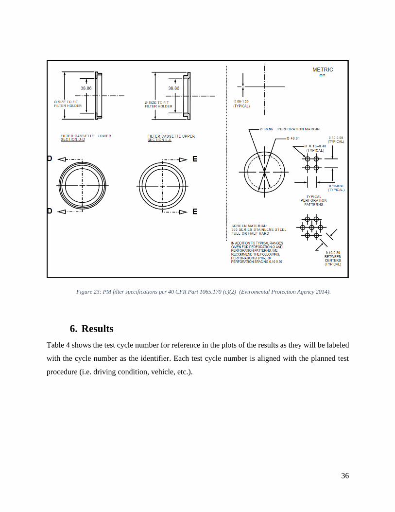
36
Figure 23: PM filter specifications per 40 CFR Part 1065.170 (c)(2) (Eviromental Protection Agency 2014).
6. Results
Table 4 shows the test cycle number for reference in the plots of the results as they will be labeled
with the cycle number as the identifier. Each test cycle number is aligned with the planned test
procedure (i.e. driving condition, vehicle, etc.).

37
Table 4: Outline of test cycle numbers with corresponding testing conditions and test vehicle.
Results are separated into PN measurement, MSS measurement, and PM collection. The sections
displaying the PN and MSS measurements have all test cycles performed plotted in the same figure
for that particle dilution ratio and the specific sampling system. The legend is displayed to the right
or bottom of the figure and it correlates the color of the trace to the test number for that test
condition. Table 4 can be used in conjunction with the figure titles and legend labels below to
further relate back to a test cycle number. Dilution ratios should project a similar affect in particle
concentrations with DR1 producing the highest concentration, followed by DR 2 which should
have half of the DR 1 particle concentration. DR 3 should have half of DR 2’s particle
concentration. This can be hypothesized because the DR 1 is diluted 2:1 for DR 2, and similarly
DR 1 is diluted 4:1 for DR 3. It can also be assumed that the dilution of DR 3 is twice that of DR
2.
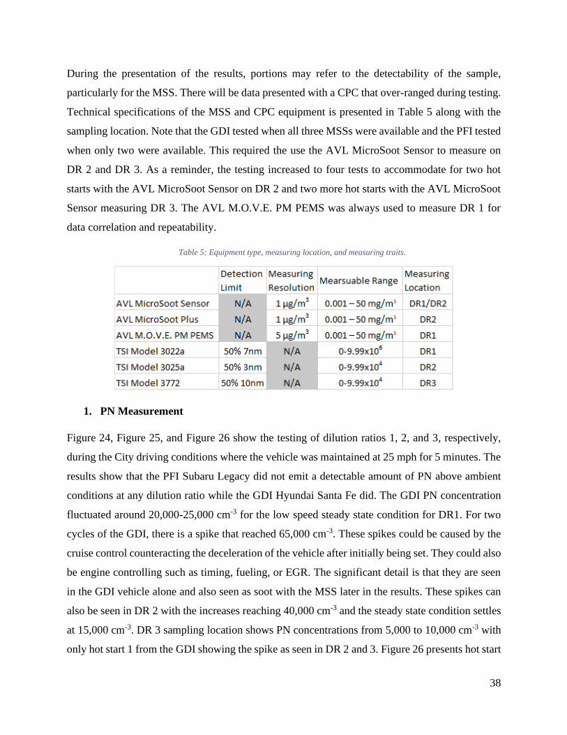
38
During the presentation of the results, portions may refer to the detectability of the sample,
particularly for the MSS. There will be data presented with a CPC that over-ranged during testing.
Technical specifications of the MSS and CPC equipment is presented in Table 5 along with the
sampling location. Note that the GDI tested when all three MSSs were available and the PFI tested
when only two were available. This required the use the AVL MicroSoot Sensor to measure on
DR 2 and DR 3. As a reminder, the testing increased to four tests to accommodate for two hot
starts with the AVL MicroSoot Sensor on DR 2 and two more hot starts with the AVL MicroSoot
Sensor measuring DR 3. The AVL M.O.V.E. PM PEMS was always used to measure DR 1 for
data correlation and repeatability.
Table 5: Equipment type, measuring location, and measuring traits.
1. PN Measurement
Figure 24, Figure 25, and Figure 26 show the testing of dilution ratios 1, 2, and 3, respectively,
during the City driving conditions where the vehicle was maintained at 25 mph for 5 minutes. The
results show that the PFI Subaru Legacy did not emit a detectable amount of PN above ambient
conditions at any dilution ratio while the GDI Hyundai Santa Fe did. The GDI PN concentration
fluctuated around 20,000-25,000 cm-3 for the low speed steady state condition for DR1. For two
cycles of the GDI, there is a spike that reached 65,000 cm-3. These spikes could be caused by the
cruise control counteracting the deceleration of the vehicle after initially being set. They could also
be engine controlling such as timing, fueling, or EGR. The significant detail is that they are seen
in the GDI vehicle alone and also seen as soot with the MSS later in the results. These spikes can
also be seen in DR 2 with the increases reaching 40,000 cm-3 and the steady state condition settles
at 15,000 cm-3. DR 3 sampling location shows PN concentrations from 5,000 to 10,000 cm-3 with
only hot start 1 from the GDI showing the spike as seen in DR 2 and 3. Figure 26 presents hot start

39
3 of the GDI. During the cycle, the GDI loses a detectable amount particle concentration until the
last minute of the cycle. From steady state low vehicle speed condition, it should be expected that
particle concentrations would be lowest of the Urban, Highway, or LA92 transient cycle
conditions. The concentration level should increase as the test conditions increase in vehicle speed.
Due to the low concentrations, the resolution of the dilution ratios was not as clear with the PN
measurement but are still seen dropping at each of the higher dilutions.
Figure 24: CPC Concentration at DR 1 during City Driving Conditions.
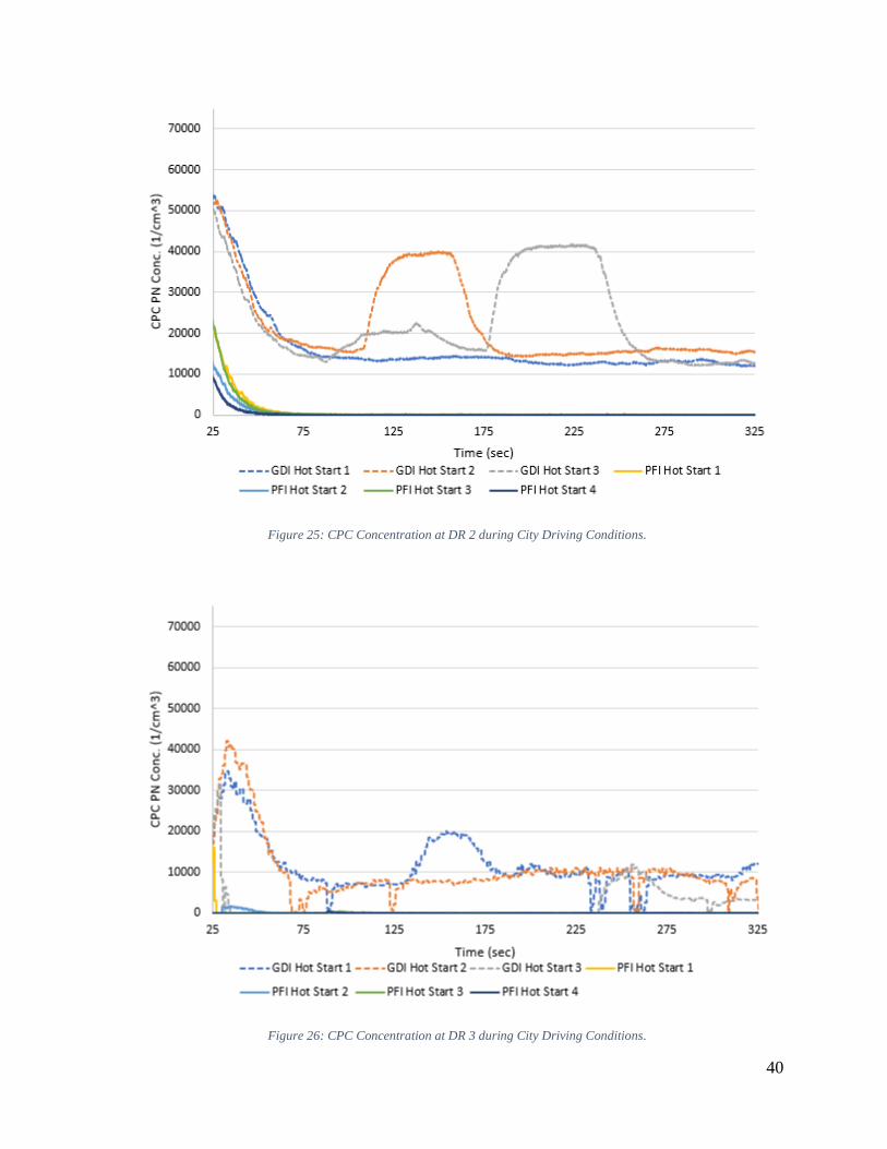
40
Figure 25: CPC Concentration at DR 2 during City Driving Conditions.
Figure 26: CPC Concentration at DR 3 during City Driving Conditions.

41
Figure 27 presents the vehicles normalized vehicle speed and CO2 traces against the DR 1 CPC
concentration to identify possible causes for the increase in concentration. Vehicle speed seems to
have no effect while CO2 shows minor signs of increasing around the increase in PN and began to
decrease shortly before the decrease of PN. This could be a possible sign of the vehicle load
increasing as cruise control begins to modulate vehicle speed. This theory is further supported in
Figure 28 with the more limited normalized axis to show vehicle speed decrease, hit the set point,
and increase. During the setpoint condition is met, the vehicle produces an increased amount of
PN.
Figure 27: Normalized Vehicle Speed and CO2 against the DR 1 CPC Concentration.

42
Figure 28: Exploded view of normalized axis of Figure 27.
Figure 29, Figure 30, and Figure 31 show the testing of dilution ratios 1, 2, and 3, respectively,
during the Urban driving conditions where the vehicle is held at 45 mph for 5 minutes. The
results are similar to the previous results with higher concentrations from the GDI and show
the trend of higher concentration with higher vehicle speed. This is to be expected because the
vehicle speed has increased, creating a larger load on the vehicle, which should yield a larger
particle number count. The GDI hot starts 2 and 3 have PN concentrations with spikes at
110,000 cm-3 and an average concentration of 55,000 cm-3 for the remainder of the cycle. Hot
start 1 GDI shows a similar trace to hot starts 2 and 3 but with a 20,000-25,000 cm-3 reduction
in particle concentration. The results for the GDI on DR 2 are like DR 1 but at half the
concentration. These results reaffirm the dilution ratio in particle concentration and as
concentration increases in the higher dilution ratio the detectability increases to involve less
variability. The DR 3 results for the GDI are similar to the City condition results with
concentrations varying from 5,000-10,000 cm-3. The PFI results remain below a detectable
concentration until hot start 4, approximately 1.5 minutes before the end, the PFI begins to
emit 6,000-8,000 cm-3 at DR 1, 1,000-3,000 cm -3 at DR 2, and 500-1,000 cm-3 at DR 3. These

43
concentrations reflect their dilution ratio with variability enough though the measured
concentrations are within the lower portion of the CPCs measurable range.
Figure 29: CPC Concentration at DR 1 during Urban Driving Conditions.

44
Figure 30: CPC Concentration at DR 2 during Urban Driving Conditions.
Figure 31: CPC Concentration at DR 3 during Urban Driving Conditions.

45
Figure 32, Figure 33, and Figure 34 show the testing of dilution ratios 1, 2, and 3, respectively,
during the Highway driving conditions where the vehicle was maintained at 65 mph for 5
minutes. During these cycles both the GDI and PFI were emitting detectable amounts of PN.
As this is the highest steady state condition, the largest PN concentration can be expected.
While the LA92 transient cycle may produce large spikes, this condition should produce the
largest constant production of particles. The GDI PN concentrations are slightly higher from
the Urban conditions for DR 1 and 2. DR 1 has a concentration of roughly 60,000 cm-3 for hot
starts 1 and 2 for the GDI. Hot start 3 for the GDI has a spike as seen in previous testing
conditions and ends the test with a large spike reaching 100,000+ cm-3, above the equipment’s
measurable range. The spike is not seen on DR 2 or 3, alluding that the spike is an equipment
or system sampling malfunction. DR 2 from the GDI testing shows concentration levels of
35,000 cm-3, slightly over half the DR 1 concentration level. DR 3 results for the GDI produce
concentrations of around 12,500 cm-3, slightly under half the concentrations of DR 2. DR 3 PN
traces also show a variability in the measurement. The PFI has a low, but detectable
concentration level beginning around 10,000 cm-3 and rising to 50,000 cm-3 consistently for
the last three tests. Hot start 1 from the PFI has a similar spike to hot start 3 from the GDI with
similar results in DR 2 and 3. The spike was not observed in the higher dilution ratios, but the
trace for hot start 3 in DR is around 1,000 cm-3 compared to the other concentrations much
higher. DR 2 for the PFI shows a PN concentrations ranging from 3,000-20,000 cm-3 for hot
start 1, 2, and 4. These tests are seen in DR 3 with concentrations around 1,000-3,000 cm-3. hot
start 3 on DR 3 shows PN concentrations two to 10 times higher than the other tests for the
PFI.

46
Figure 32: CPC Concentration at DR 1 during Highway Driving Conditions.
Figure 33: CPC Concentration at DR 2 during Highway Driving Conditions.

47
Figure 34: CPC Concentration at DR 3 during Highway Driving Conditions.
Figure 35, Figure 36, and Figure 37 provide the results from the CPCs during the LA92 drive
cycle. These three figures used a log scale for PN concentration to reflect the magnitude of particle
production more accurately. One test for the GDI was performed while two tests were performed
on the PFI to allow for the AVL MSS to be moved from DR2 to DR3. The results of these cycles
show spikes in DR1 reaching higher than 250,000 cm-3 and sustained concentrations of 150,000
cm-3 from the GDI. The DR 2 shows slightly under half the concentration of DR 1, while DR 3
shows half of the concentration of DR 2. The spikes are not seen as the resolution of the particle
concentration is lost through dilution. A significant observation is that the PFI and GDI have
similar concentration levels until the load is sustained. During this period between 300-500
seconds the GDI still produces a large concentration of PN while the PFI may only show a large
spike of 600,000 cm-3 (compared to 100,000 cm-3 spikes of the GDI) and back down to 20,000
cm-3. Another instance at 870-960 seconds the PFI produces a series of spikes that over range the
CPC. These results are also seen in DR 2 and 3. Particularly in DR 3 at ~900 seconds and ~1000
seconds the CPC over ranges as shown in Figure 37 (CPC technical specifications in Table 5).
Another observation is the GDI engine producing large spikes of PN concentration under
conditions of load during the cycle. When comparing the results from the McCaffery study in
Figure 3, there was discussion of a high PN concentration for the Mt. Baldy route (McCaffery, et

48
al. 2019). During the cycle, the spray guided GDI vehicle produced four times the PN
concentrations of the wall guided. During the LA92 test cycle in this research, the GDI emitted
constant levels of PN concentrations under portions of the LA92 cycle that required heavy
accelerations. These portions would be similar to the Mt. Badly test route could be a possible
correlation in particle emission of spray guided GDI engines under heavy load.
Figure 35: CPC Concentration at DR 1 during LA92 Driving Cycle.
Figure 36: CPC Concentration at DR 2 during LA92 Driving Cycle.
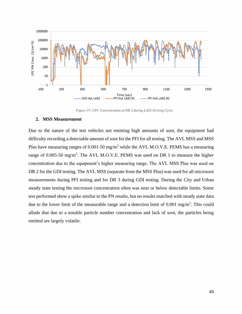
49
Figure 37: CPC Concentration at DR 3 during LA92 Driving Cycle.
2. MSS Measurement
Due to the nature of the test vehicles not emitting high amounts of soot, the equipment had
difficulty recording a detectable amount of soot for the PFI for all testing. The AVL MSS and MSS
Plus have measuring ranges of 0.001-50 mg/m3 while the AVL M.O.V.E. PEMS has a measuring
range of 0.005-50 mg/m3. The AVL M.O.V.E. PEMS was used on DR 1 to measure the higher
concentration due to the equipment’s higher measuring range. The AVL MSS Plus was used on
DR 2 for the GDI testing. The AVL MSS (separate from the MSS Plus) was used for all microsoot
measurements during PFI testing and for DR 3 during GDI testing. During the City and Urban
steady state testing the microsoot concentration often was near or below detectable limits. Some
test performed show a spike similar to the PN results, but no results matched with steady state data
due to the lower limit of the measurable range and a detection limit of 0.001 mg/m3. This could
allude that due to a notable particle number concentration and lack of soot, the particles being
emitted are largely volatile.

50
Figure 38: MSS Concentration at DR 1 during City Driving Conditions.
Figure 39: MSS Concentration at DR 2 during City Driving Conditions.

51
Figure 40: MSS Concentration at DR 3 during City Driving Conditions.
Figure 41: MSS Concentration at DR 1 during Urban Driving Conditions.

52
Figure 42: MSS Concentration at DR 2 during Urban Driving Conditions.
Figure 43: MSS Concentration at DR 3 during Urban Driving Conditions.
The Highway steady state condition shows a average microsoot concentraion of .01 mg/m3 for the
GDI while the PFI produced a concentration below the detectable limit. As previously seen in the
PN results, the DR 2 concentration is half of DR 1. DR 3 shows a concentraion of 0.015 mg/m3
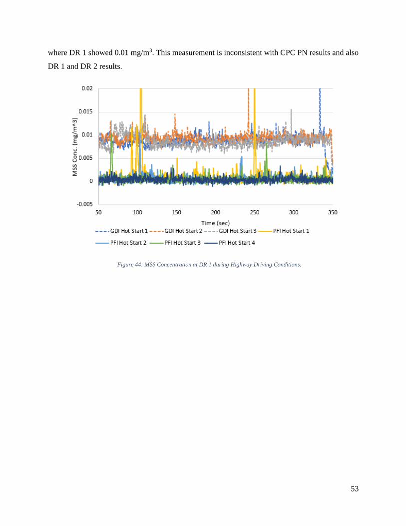
53
where DR 1 showed 0.01 mg/m3. This measurement is inconsistent with CPC PN results and also
DR 1 and DR 2 results.
Figure 44: MSS Concentration at DR 1 during Highway Driving Conditions.

54
Figure 45: MSS Concentration at DR 2 during Highway Driving Conditions.
Figure 46: MSS Concentration at DR 3 during Highway Driving Conditions.
MSS results from the LA92 drive cycle on DR 1 show the GDI sustaining higher concentrations
in the first half of the cycle while the PFI had large spikes that settled near the detection limit of

55
0.001 mg/m3. Spikes of concentration measured up to 9 mg/m3 at 500 seconds during LA92 of the
PFI where the GDI only increased to 0.5 mg/m3. The concentration of microsoot measured from
the GDI before and after the spike is an order of 10 to 20 times higher than that of the PFI. This
data is presented in Figure 47. During the second half of the LA92 cycle the GDI and PFI microsoot
traces remain within 0.005 mg/m3 each other. While the spikes of the PFI remain 10 to 20 higher
than the GDI, the concentration settles close to the detection limit when not under load, shown in
Figure 48.
Figure 47: MSS Concentration at DR 1 during the first half of the LA92 Driving Conditions.
Figure 48: MSS Concentration at DR 1 during the second half of the LA92 Driving Conditions.
The measurement with the MSS at DR 2 is shown over the full cycle in Figure 49 and broken into
two halves again in Figure 50 and Figure 51. As seen in Figure 49, the PFI microsoot concentration
rises during the spikes seen in Figure 47 and Figure 48. During the spikes it appears the

56
concentration lingers and causes the MSS to measure a saturated sample. In Figure 50 at 350
seconds, there is a initial spike and the concentration reduces to low range limit of the MSS for the
PFI while the GDI trace remains near 0.005-0.01 mg/m3. This behavior is also seen Figure 35,
Figure 36, and Figure 37 measuring PN with the CPCs. The MSS data may be compromised at
high dilution ratios due to a saturated sample during high particle mass spikes in the PFI testing.
Figure 49: MSS Concentration at DR 2 during the LA92 Driving Conditions.
Figure 50: MSS Concentration at DR 2 during the first half of the LA92 Driving Conditions.
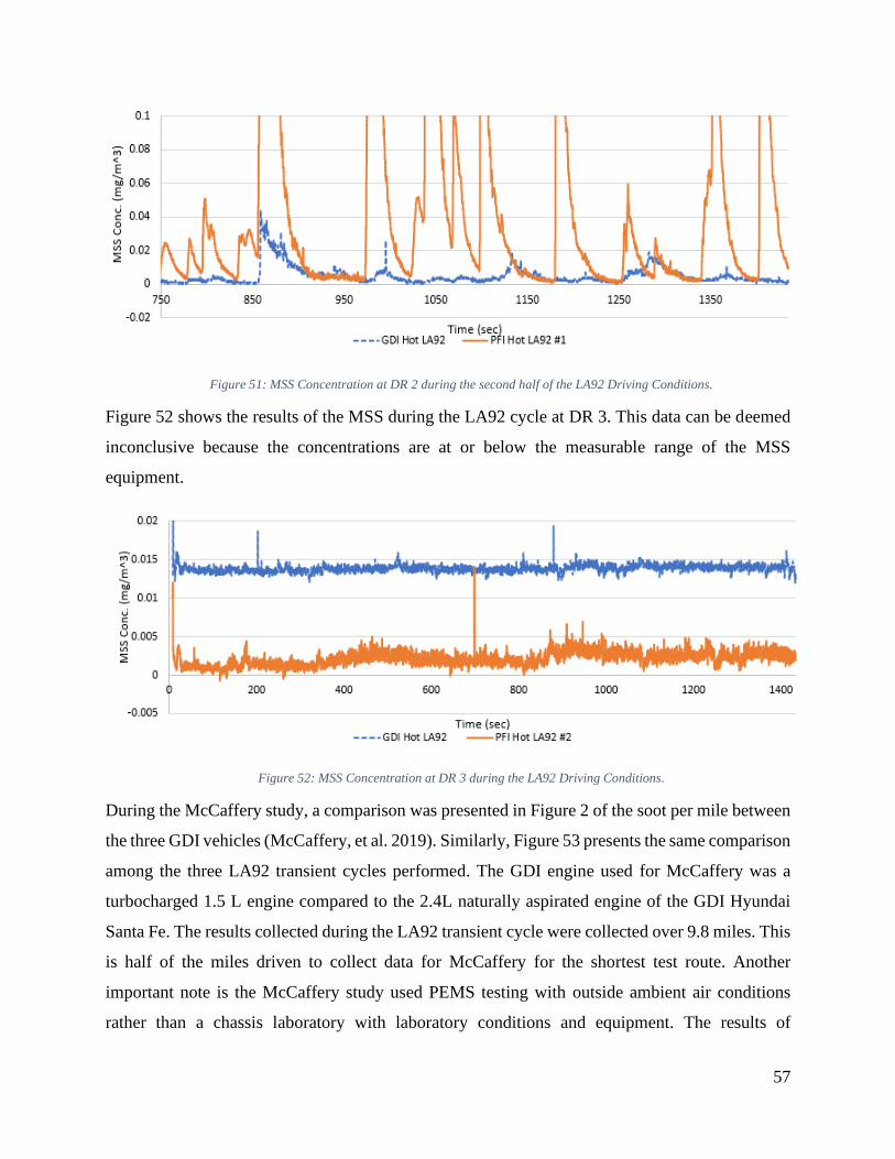
57
Figure 51: MSS Concentration at DR 2 during the second half of the LA92 Driving Conditions.
Figure 52 shows the results of the MSS during the LA92 cycle at DR 3. This data can be deemed
inconclusive because the concentrations are at or below the measurable range of the MSS
equipment.
Figure 52: MSS Concentration at DR 3 during the LA92 Driving Conditions.
During the McCaffery study, a comparison was presented in Figure 2 of the soot per mile between
the three GDI vehicles (McCaffery, et al. 2019). Similarly, Figure 53 presents the same comparison
among the three LA92 transient cycles performed. The GDI engine used for McCaffery was a
turbocharged 1.5 L engine compared to the 2.4L naturally aspirated engine of the GDI Hyundai
Santa Fe. The results collected during the LA92 transient cycle were collected over 9.8 miles. This
is half of the miles driven to collect data for McCaffery for the shortest test route. Another
important note is the McCaffery study used PEMS testing with outside ambient air conditions
rather than a chassis laboratory with laboratory conditions and equipment. The results of

58
McCaffery’s study show their spray guided GDI as emitting more than the two wall guided
engines. The LA92 cycles performed with the GDI produced less soot per mile than the PFI in
both cycles by an average of 0.01 mg/mile. In the comparison to the McCaffery study, the GDI
engine produced similar amounts of soot to the spray guided GDI vehicle after the catalyzed GPF
was installed.
Figure 53: Soot per Mile during the LA92 transient cycle>
3. PM Collection
The PM data collection utilized versatile PM equipment that could be used in various sampling
systems. The orifices used to control flow were able to achieve the maximum filter face velocity
allowed by CFR 40§1065.170(a)(2). This section of the CFR describes the filter flow velocity to
be set to 50 cm/s but only if the filter loading is exceeding a target of 400 μg. This design
requirement of the PM boxes made gravimetric measurement difficult at high dilution ratios and
in sampling environments where PM loading is not significant. The vehicles are regulated to a PM
emissions standard of 0.01 g/mi, deeming them to be a low emitting vehicle and combined with
the high dilution ratios the results from the PM collection are inconclusive and do not correlate
with the AVL MSS equipment. The results from the testing can be found in the Appendix and
recommendations for a repeat test setup will be suggested in the Recommendations.

59
7. Conclusions
The results showed the PFI engine of the Subaru Legacy tended to emit lower particle
concentrations but not soot compared to the GDI engine of the Hyundai Santa Fe. This was shown
in the results taken with the CPC and the microsoot sensor measurements. While on average, the
GDI vehicle produced more PN concentration and soot during the steady state; the PFI produced
a higher average soot/mile during the transient LA92 cycle. During each steady state condition,
the GDI produced an average PN concentration of 25,000 cm-3 during the City condition at DR 1
while the PFI’s PN concentration was not detectable. During the Urban condition, the GDI
produced 35,000-45,000 cm-3 while the PFI consistently produced a spike of 8,000 cm-3 that
lowered to 2,000 cm-3 and rose back to 6,000 cm-3 near the end of the cycle at DR 1. During the
Highway condition of the steady state testing at DR 1 the GDI produced 55,000-60,000 cm-3 as
the PFI produced 10,000 cm-3 and increased during the cycle to end with 40,000 cm-3 to 60,000
cm-3. The MSS data revealed similar results but with both vehicles yielding concentrations near
the lower detection limit (LDL) of the microsoot sensor. The GDI shows a small spike near the
beginning of the steady state cycles but both the GDI and the PFI produced soot concentrations
too low to make a data supported conclusion. This also explained the results seen with the PM,
without any soot being produced, the PM mass failed to yield conclusive results. While there was
minimal soot to measure any detectable levels of PN concentration, it could be assumed the
majority of the particles produced would be considered volatile. Inconclusive PM mass with
repeatable PN measurement is an example why a PN style measurement should be implemented
to aid in future emissions standards. During the transient test measuring with CPCs, the GDI engine
produced more particles during operation while the PFI engine produced extremely high spikes
that would be near the detection limit of the equipment. These spikes caused the PFI engine to
produce twice the PN average as the GDI engine. A discrepancy with the CPC data could be the
minimum particle size detection. The TSI 3025A had a 50% detection limit at 3 nm particle size,
the while the TSI 3022A and TSI 3772 had 50% detection limits at 7 nm particle size. This could
allow for the TSI 3022A to measure more particles than the other CPCs and because TSI 3022A
was measuring at DR 1, it could contribute to such high spikes of PN. Another issue is these
particles are solid and non-solid. Without an evaporator tube or catalyst to remove non-solid
particle, these measurements were elevated compared to a solid particle measurement completed
with other equipment. MSS measurements also showed similar results to the CPC. As the dilution

60
ratio increased, the measurements tended towards the limiting resolution of the sensors. This is
shown during large spikes from the PFI engine at DR1 that is orders of magnitude higher than GDI
and when comparing the DR2 traces, the measurement of the PFI and GDI was on the same order
of magnitude.
8. Recommendations
Recommendations for similar testing include a larger pool of vehicles to evaluate as only a spray
guided GDI engine was tested. A wall-guided GDI, a PFI-GDI, and a wall/spray-guided GDI
would allow more data to draw conclusions on the injection technologies. Due to low staffing
during testing, the drivers for the two vehicles were different and inexperienced. Having a single
experienced driver would reduce variability in following the transient speed trace on the
dynamometer, producing more consistent results. Another recommendation would be to integrate
a TSI EEPS and AVL APC or equivalent equipment at all the sampling locations. Doing this would
allow for a measurement of particle distribution for each engine type and how it may or may not
change with different dilution ratio environments. The AVL APC could measure a solid particle
number concentration at each sample location to better understand how many of the non-solid
particles are lost in the transition to each of the dilution ratios. These results could conclude if high
dilution sampling would cause too significant losses of amount of particle to be a valid option for
particle measurement. For PM sampling, the flow should be increased to target a 400 μg loading
rather than use a universal PM box. Although increasing sample flow may have various effects on
isokinetic flow of the sampling tunnels. Increasing sampling flow may also require an increase in
filter size to prevent excessive filter face velocity. Another method to increase loading would be
to increase sampling time. This may help for higher vehicle speed conditions, but low speed
sampling may still not yield any particulates without extensive data collection periods. From the
data collected, once the PFI had achieved the steady state condition it will not produce a PN
concentration unless under load. Rather than using a speed condition as a metric, an emphasis on
load should be considered. Using longer sampling times would also include back to back cycles
for transient cycles. This would give a more meaningful results and could better reinforce a
conclusion. Ideally the dilution integration and sampling tunnels would be identical rather than
having long sample lines, separate geometries for the mixing tunnels, different equipment with
different specifications.

61
9. Appendix
Figure 54: O'Keefe Controls Co. Orifice Data Sheet for Metal Orifice Air Flow in SCFM.

62
Figure 55: PM Weights from Hyundai Santa Fe Tests.

63
Figure 56: PM Weights from Subaru Legacy Tests 1 of 2.
Figure 57: PM Weights from Subaru Legacy Tests 2 of 2.

64
Figure 58: Gravimetric Mass results from City Conditions with the Hyundai.
Figure 59: Gravimetric Mass results from City Conditions with the Subaru.

65
Figure 60: Gravimetric Mass results from Urban Conditions with the Hyundai.
Figure 61: Gravimetric Mass results from Urban Conditions with the Subaru.

66
Figure 62: Gravimetric Mass results from Highway Conditions with the Hyundai.
Figure 63: Gravimetric Mass results from Highway Conditions with the Subaru.

67
Figure 64: Gravimetric Mass results from LA92 drive cycle with the Hyundai.
Figure 65: Gravimetric Mass results from LA92 drive cycle with the Subaru.

68
Figure 66: Aerial View Empty Test Cell with Multi-Dilution Setup Installed.
Figure 67: Side View Empty Test Cell with Multi-Dilution Setup Installed #1.

69
Figure 68: Side View Empty Test Cell with Multi-Dilution Setup Installed #2.
Figure 69: Overview of Control Room for Test Cell.
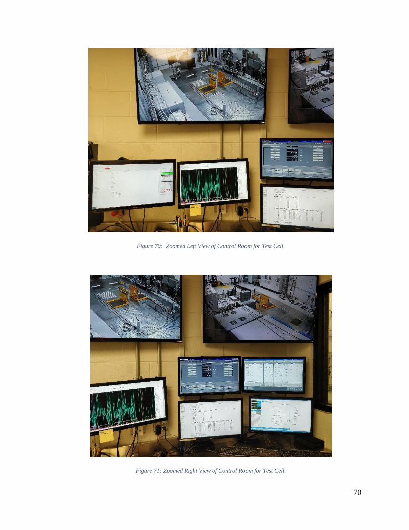
70
Figure 70: Zoomed Left View of Control Room for Test Cell.
Figure 71: Zoomed Right View of Control Room for Test Cell.

71
Figure 72: Gas Bottle Rack Containing Span Gases for Analyzers on Test Stand.
Figure 73: Uncovered View of Wall-Mounted DAQ Box with Test Cell Edgetech Humidity Sensor.

72
Figure 74: Covered View of Wall-Mounted DAQ Box with Test Cell Edgetech Humidity Sensor.
Figure 75: Box B PM Box with door shut.

73
Figure 76: Wiring of the Temperature Controllers for PM Box B.
Figure 77: Box B PM Box with door open.

74
Figure 78: Zoomed in View of the Internals of PM Box B.

75
Figure 79: Side View of the Third Dilution Tunnel, DR 3 Analyzer Rack Test Stand, and PM Box A.

76
Figure 80: Zoomed in View of the Internals of PM Box A.

77
Figure 81: Closer of the DR 3 Dilution Tunnel (most right tunnel).

78
Figure 82: Zoomed Front Left View of the Analyzer Rack Test Stand.

79
Figure 83: Front View of the Analyzer Rack Test Stand.
Figure 84: Zoomed View of the DR 3 Ejector Dilutor and Mass Flow Controller.

80
Figure 85: DR 3 and Raw CO2 Analyzers with the Switchboard to Zero/Span/Sample Above.
Figure 86: FID Analyzer used to perform Propane Injections for DR 3 Dilution Confirmation.

81
Figure 87: Isotropic View without Cover of the DAQ Box mounted on the Analyzer Rack Test Stand.
Figure 88: Front View with Cover of the DAQ Box mounted on the Analyzer Rack Test Stand.

82
Figure 89: ICP-CON #2 in DAQ Box mounted on Analyzer Rack Test Stand.
Figure 90: ICP-CON #1 in DAQ Box mounted on Analyzer Rack Test Stand.

83
Figure 91: Power Supply for Equipment in DAQ Box on Analyzer Rack Test Stand.
Figure 92: StarTech to connect CPC's, MSS's, and MFC's in DAQ Box on Analyzer Rack Test Stand.
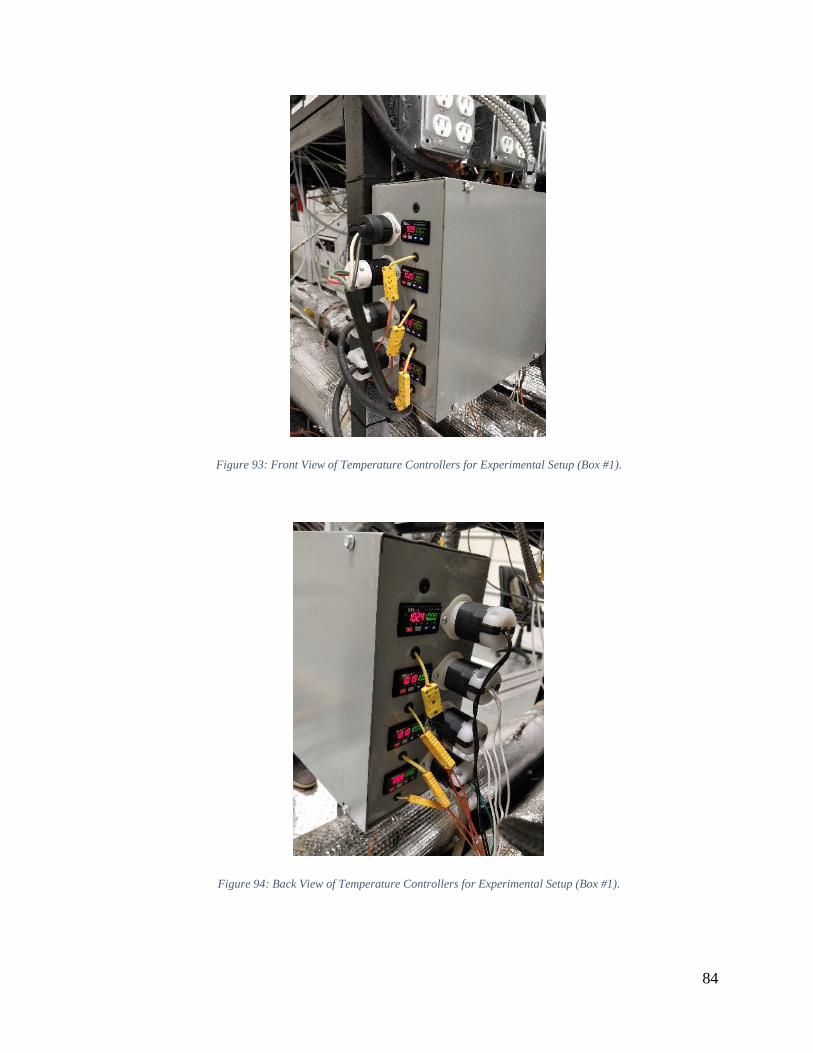
84
Figure 93: Front View of Temperature Controllers for Experimental Setup (Box #1).
Figure 94: Back View of Temperature Controllers for Experimental Setup (Box #1).

85
Figure 95: Uncovered Side View of Temperature Controllers for Experimental Setup (Box #1).

86
Figure 96: Front View of Temperature Controllers for Experimental Setup (Box #2).
Figure 97: Uncovered Side View of Temperature Controllers for Experimental Setup (Box #2).

87
Figure 98: Dilution Tunnel for DR 2 with the DR 2 PM Box (DLMB) in the back.

88
Figure 99: Dilution Tunnel for DR 2, Top View.
Figure 100: Horiba OBS-ONE used to Sample on DR 2 with Span/Zero Cal Gasses on Bottle Rack.
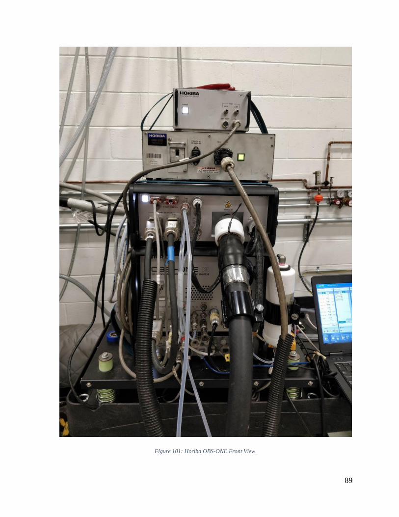
89
Figure 101: Horiba OBS-ONE Front View.

90
Figure 102: Horiba OBS-ONE Zoomed Side View.

91
Figure 103: Horiba OBS-ONE Software Computer.

92
Figure 104: Overview of the Test Cell with the Hyundai Test Vehicle.
Figure 105: Rear View of the Test Cell with the Hyundai Test Vehicle.

93
Figure 106: Side Rear View of the Test Cell with the Hyundai Test Vehicle.
Figure 107: Front Top View of the Test Cell with the Hyundai Test Vehicle.

94
Figure 108: Image #1 of all Equipment in place during the Hyundai Testing.

95
Figure 109: Image #2 of all Equipment in place during the Hyundai Testing.
Figure 110: Image #3 of all Equipment in place during the Hyundai Testing.

96
Figure 111: Image #4 of all Equipment in place during the Hyundai Testing.

97
Figure 112: Image #1 of the Test Cell During the Subaru Testing.

98
Figure 113: Image #2 of the Test Cell During the Subaru Testing.
Figure 114: Image #3 of the Test Cell During the Subaru Testing.
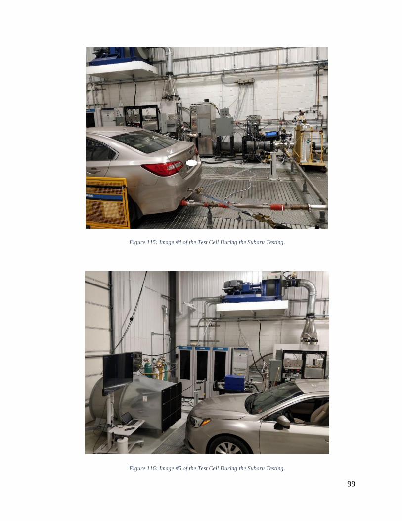
99
Figure 115: Image #4 of the Test Cell During the Subaru Testing.
Figure 116: Image #5 of the Test Cell During the Subaru Testing.

100
Figure 117: Image #6 of the Test Cell During the Subaru Testing.
Figure 118: Image #7 of the Test Cell During the Subaru Testing.
101
10. References
Air-Vac. 2011. Air-Operated Vacuum Pumps. January 25. Accessed June 3, 2020.
https://www.airvacpumps.com/AVstainless.html.
Awad, Omar I., Xiao Ma, Mohammed Kamil, Zhou Zhang Obed Majeed Ali, and Shijin Shuai.
2020. "Particulate emissions form gasoline firect injetion engines: A review of how current
emissions regulations are being met by automobile manufacturers." Science of the Total
Enviroment 718: 0-17.
Besch, Marc. Cyrill. 2016. In-line, Real-time Particulate Matter Sensors for OBD and Exhaust
After-treatment System Control Applicaitons. PhD Disseratation, Morgantown, WV:
Departmnet of Mechanical and Aerospace Engineering.
ECE/TRANS/505/Rev.7/Add.48. 2015. "Agreement, Addendum 48: Regulation No. 49, Revision
7."
EPA, Office of Transprotation and Air Quality's. 2020. The 2019 EPA Automotive Trends Report.
EPA Automotive Trends Report, Ann Arbor: United States Enviromental Protection
Agency.
Eviromental Protection Agency. 2014. "Federal Register." Control of Air Pollution From Motor
Vehicles: Tier 3 Motor Vehicle Emissions and Fuel Standards; Final Rule. Vol. 79.
National Arcihves and Records Administration, April 28. Accessed May 1, 2020.
https://www.govinfo.gov/content/pkg/FR-2014-04-28/pdf/2014-06954.pdf.
GCC. 2006. Mercedes-Benz Premiers New Gasoline Direct Injection System for More Power and
Lower Fuel Consumption. Feburary 24. Accessed 5 26, 2020.
https://www.greencarcongress.com/2006/02/mercedesbenz_pr.html.
Heywood, John B. 1988. Internal Combustion Engine Fundamentals. McGraw-Hill Publishing
Company.
Karavalakis, Georgios, Daniel Short, Diep Vu, Robert L. Russell, Akua Asa-Awuku, Heejung
Jung, Kent C. Johnson, and Thomas D. Durbin. 2015. "The impact of ethanol and iso-
butanol blends on gaseous and particulate emissions from two passenger cars equipped

102
with spray-guided and wall-guided direct injection SI (spark ignition) engines." Energy
168-179.
Kittelson, David B. 1998. "Engines and Nano Particles: A Review." Journal of Aerosol Science
575-588.
Ko, Jinyoung, Kangjin Kim, Cha-Lee Myung Wonyong Chung, and Simsoo Park. 2018.
"Characteristics of on-road particle number (PN) emissions from a GDIvehicle depending
on a catalytic stripper (CS) and a metal-foam gasolineparticulate filter (GPF)." Fuel 363-
374.
Ko, Jinyoung, Kangjin Kim, Wonyong Chung, Cha-Lee Myung, and Simsoo Park. 2018.
"Characteristics of on-road particle number (PN) emissions from a GDI vehicle depending
on a catalytic stripper (CS) and a metal-foam gasoline particulate filter (GPF)." Fuel
(Elsevier) 363-374.
McCaffery, Cavan, Hanwei Zhu, Chengguo Li, Thomas D. Durbin, Kent C. Johnson, Heejung
Jung, Rasto Brezny, Michael Geller, and Georgios Karavalakis. 2019. "On-road gaseous
and particulate emissions from GDI vehicles with and without gasoline particulate filters
(GPFs) using portable emissions measurement systems (PEMS)." Science of the Total
Enviroment.
Meriam. n.d. "User Manual Laminar Flow Elements." https://www.meriam.com/. Accessed 11 30,
2020. https://www.meriam.com/assets/LFE-User-Manual.pdf.
Moon, Seoksu, Tianyun Li, Kiyotaka Sato, and Hideaki Yokohata. 2017. "Governing parameters
and dynamics of turbulent spray atomization from modern GDI injectors." Energy 89-100.
O'Keefe Controls Co. 2003. "Precision Metal Orifices - NPT Hex Nipple - Choked Flow of Gases."
O'Keefe Controls Co. Web Site. Accessed June 6, 2020.
https://catalog.okeefecontrols.com/viewitems/precision-metal-orifices-npt-
connections/precision-metal-orifices-npt-hex-nipple.
—. 2011. "Precision Metal Orifices - NPT Hex Nipple - Technical Considerations." O'Keefe
Controls Co. Web Site. Accessed June 6, 2020.

103
https://catalog.okeefecontrols.com/viewitems/precision-metal-orifices-npt-
connections/precision-metal-orifices-npt-hex-nipple.
Raza, Mohsin, Longfei Chen, Felix Leach, and Shiting Ding. 2018. "A Review of Particle Number
(PN) Emissions from Gasoline Direct Injection (GDI) Engines and Their Control
Techniques." Energies 1-26.
Saito, Chika, Takahiko Nakatani, Y. Miyairi, Kazuya Yuuki, Mikio Makino, Hiroshi Kurachi,
Wolfgang Heuss, et al. 2011. "New Particulate Filter Concept to Reduce Particle Number
Emissions." SAE Technical Paper, No. 2011-01-0814.
Shouse, Kate C., and Richard K. Lattanzio. 2020. Clean Air Act: A Summary of the Act and Its
Major Requirements. Congressional Research Service.
Sydbom, A., A. Blomberg, S. Parnia, N. Stenfors, T. Sandstorm, and S-E Dahlén. 2001. "Health
effects of diesel exhaust emissions." European Respiratory Journal 733-746.
Zhao, Hua. 2009. Advanced Direct Injection Combustion Engine Technologies and Development.
Woodhead Publishing.