investigation of pressurized wave bearings

Final Technical Report

for

Investigation of Pressurized Wave Bearings

NASA Grant Number NAG3-2408

Grant Duration April 18,2000 to December 3 1,2003

Dr. The0 G. Keith, Jr. Principal Investigator

Florin Dimofte Co-Principal Investigator

Department of Mechanical, Industrial and Manufacturing Engineering University of Toledo Toledo, Ohio 43606

December 2003

Final Report for NASA grant NAG3-2408

Investigation of Pressurized Wave Bearings

The0 G. Keith, Jr. (Distinguished University Professor) Florin Dimofte (Senior Research Associate)

Department of Mechanical, Industrial and Manufacturing Engineering The University of Toledo, Toledo, Ohio 43606

PURPOSE This grant supported research on gas (air) wave bearings for turbomachinery applicaf;-ons. A team nf researchers from the U~iversity of Toledo performed the research. The team consists of Dr. The0 Keith (Distinguished University Professor), Dr. Florin Dimofte (Senior Research Associate) and Sorin Cioc (PhD Research Assistant).

INTRODUCTION The wave bearing has been pioneered and developed by Dr. Dimofte over the past several years. This bearing will be the main focus of this research. It is believed that the wave bearing offers a number of advantages over the foil bearing, which is the bearing that NASA is currently pursuing for turbomachinery applications.

The wave bearing is basically a journal bearing whose film thickness varies around the circumference approximately sinusoidally, with usually 3 or 4 waves. Being a rigid geometry bearing, it provides precise control of shaft centerlines. The wave profile also provides good load capacity and makes the bearing very stable. Manufacturing techniques have been devised that should allow the production of wave bearings almost as cheaply as conventional full-circular bearings.

RESEARCH ACCOMPLISHMENTS

The research performed on this grant is described in the following 4 papers:

1. “Measured Gas Wave Journal Bearing Load Capacity at Steady Loads,” (co-authors: F. Dimofte, and D.P. Fleming), presented at the 9* International Symposium on Transport Phenomena and Dynamics of Rotating Machinery (ISROMAC-9), Honolulu, Hawaii, February 10-14,2002

c

2. "Computation of Pressurized Gas Bearings Using CE/SE Method," (co-authors: S. Cioc, F. Dimofte, and D. P. Fleming) STLE Tribology Transactions Vol. 46, No. 1, January 2003, pp 128- 13 3.

3. "Application of the CE/SE Method to Wave Journal Bearings," (co-authors: S. Cioc, and F. Dimofte) STLE Tribology Transactions Vol. 46, No. 2, April 2003, pp. 179-186.

4. "Calculation of the Flow in High Speed Gas Bearings Including Inertial Effects Using the CE/SE Method," (co-authors: S. Cioc, F. Dimofte, and D. P. Fleming) presented at the 58th STLE Annual Meeting in New York, New York, April 28 - May 1,2003

A copy of each of the first three papers is included below. Because the last paper is under review for publication in the STLE Tribology Transactions it is not included in this report.

* 9"' International Symposium on Transportation Phenomena

Honolulu, Hawaii, February 10-14,2002

---I n..---:-- -c a-c,+:.., am-..^:....^, ~ I I U Y~I I~ I I I ILJ UI nuLaritiy i v i a ~ i i ~ i ~ c ~ y

MEASURED GAS WAVE JOURNAL BEARING LOAD CAPACITY UNDER STEADY LOADS.

Florin Dimofte, The University of Toledo, currently working at NASA Glenn Research Center, Cleveland, Ohio,

David P. Fleming, NASA Glenn Research Center, Cleveland, Ohio,

The0 G. Keith, Jr., The University of Toledo.

ABSTRACT

A 'X mm rliarnetpr hv 28 !"nu \.yaw- air bea.ing w s a -.- --- , . d., L L... L V.U..%..,L .,>

tested at speeds up to 30,000 rpm. The tests were performed on a gas bearing rig at NASA Glenn Research Center in Cleveland, Ohio. A maximum load of 196 N was supported by the bearing at maximum speed for more than 90 minutes. The bearing was stable both dynamically and thermally. Good agreement was found with numerical prediction.

INTRODUCTION

A circular (plain) journal bearing has better load capacity than all other hydrodynamic journal bearings if the comparison criteria is the minimum film thickness. However, the plain journal bearing is easily de-stabilized, especially if the bearing is unloaded. This has been proven both theoretically and experimentally [l, 2,3]. To improve stability, the plain journal bearing's geometry must be modified.

Numerous concepts including lobed, grooved, stepped, and tilting-pad bearings were developed. These concepts, however, have substantially lower load capacity. The wave bearing, a new concept developed at NASA Glenn Research Center, offers good stability with a load capacity that is close to that of a plain journal bearing [4]. The wave journal bearing features a wave profile circumscribed on the inner bearing diameter. The wave bearing can have 2, 3 or more waves, and the wave amplitude can vary. However a three wave bearing was found to better satisfy both steady-state and dynamic running conditions than other wave bearing geometries [ 5 , 61. A three-wave bearing concept is shown in fig. la. A plain journal bearing is shown in fig. lb for comparison. The wave amplitude and bearing clearance are exaggerated so that the wave profile can be seen.

Predictive analysis was developed to quantify the performance of wave journal bearings and contrast it to plain

journal bearings [4]. The predictions revealed a significant difference in the pressure distribution between the three-wave and the plain journal bearing. The altered pressure distribution p v i d e s a higher !oad c,ilpacity for the wave bearing when compared to the plain circular bearing operating at the same eccentricity [4]. In addition, the wave journal bearing offers better stability. The analysis was performed assuming that the bearings were operating in air, a compressible lubricant. This analysis was validated by the measurements performed on a bench test rig that was assembled at NASA Glenn Research Center [7]. The work presented herein was performed to establish the practical maximum load capacity of a wave bearing that could also be compared to other types of air bearings.

DESCRIPTION OF TEST RIG

An air bearing test rig (fig. 2) was built to test journal bearings with 30-50 mm diameters and 25-60 mm lengths. A commercial air spindle (fig. 2, pos. 4) with a removable add-on shaft is used to drive the test bearing. It is mounted vertically to eliminate gravitational effects. The spindle can operate at rotational speeds to 30,000 rpm with a shaft run-out of less than 40 micro-inches (1 micron). A cross section of the bearing assembly is presented in fig. 3. The mechanical run-out of the add-on shaft (fig. 3, pos 4) was measured with a contact electronic dial indicator, accurate to 0.1 pm. The run-out of the add-on shaft is less than 0 . 2 pm at the top (farthest from the spindle) and less than 0. 1 pm at the bottom (closest to the spindle).

The test bearing set up can be seen in fig. 4. The test bearing housing (fig. 3, pos. 1 or fig. 4, pos. 1 ) is supported between two air thrust plates (fig 4, pos.2 and 3). The thrust plates allow the test bearing to move freely in the radial direction. The bottom thrust plate (fig. 4, pos. 2) was designed with 3 thrust pads to allow bearing alignment to the shaft. Each pad has a separate air suppiy system inciuding a valve (regulator) and pressure gauge. The top thrust plate (fig. 4, pos.3) contains a single 360 degree pad. It is supported by three threaded rods (fig. 4, pos. 4) which allow easy adjustment to the axial clearance of both (bottom and top) thrust

1

* plates. CONCLUDING REMARKS

The bearing rotor (fig. 3, pos. 5) is mounted on the top of the add-on shaft. The bearing sleeve is assembled inside the bearing sleeve assembly (fig. 3, pos. 2). The bearing sleeve assembly is fixed inside the housing (fig. 3, pos. 1). Rubber O-rings are used between the bearing sleeve assembly and the housing to provide additional self- alignment capability when load is applied. The test bearing was operated in ambient air.

A radial load can be applied to the test bearing via a pneumatic load cylinder (fig.2, pos. 2). A micro-switch (fig. 4, pos. 5) is used to sense excessive torque on the bearing housing; it will shut off the spindle if triggered. A burst shield surrounds the experimental bearing for added safety.

The test rig includes instrumentation to measure shaft speed, radial load, rotor-sleeve position, and bearing temperature. Shaft speed is measured by a capacitive probe h x i e b within the spindle. A iiiiniaiure precision ioad ceii (fig. 2, pos. 3 or fig. 4, pos. 6) measures the radial load applied by the pneumatic load cylinder. Two light beam displacement sensors (fig. 4, pos. 7) allow measurement of rotor-sleeve position. The bearing housing temperature is monitored with K-type thermocouples (fig. 4, pos. 8).

TEST RESULTS

The tested bearing has a 35 mm diameter and is 28 mm long. The radial clearance was 18 p m and the ratio of the wave amplitude to radial clearance is 0.143. Since the goal of this work was to establish a maximum practical load capacity of the wave journal bearing, the bearing was tested under relatively large loads. Consequently, large eccentricity to radial clearance ratios (greater than 0.7) resulted. Speeds of 5000, 10,000, 20,000, and 30,000 rpm were used. Eccentricity, shaft speed, and load were recorded at each load step by using a digital camera. A typical photograph containing this information can be seen in fig. 5. This figure also shows the maximum load applied to the bearing in this test, 44 lb (196 N), at a maximum shaft speed of 29,418 rpm where the bearing operated with 15.8 pm eccentricity. The bearing temperature was also monitored. At maximum speed the bearing temperature stabilized at 33OC in a few minutes and was then virtually constant throughout the tests, which ranged up to 90 minutes.

The results of this test are plotted in fig. 6 in terms of specific load (average bearing pressure) versus eccentricity ratio. Analytical predictions are also plotted. Figure 6 shows that the wave bearing ran at eccentricity ratios from 0.7 to 0.88 The bearing run stably at all speeds, and bearing temperature stabilized in a short time at reasonable values for each run. The wave bearing can cany a specific load of 2 bars at 30,000 rpm.

A 35 rnm diameter by 28 mm long wave air bearing was tested at speeds up to 30,000 rpm in the hydrodynamic regime. The test was performed on the gas bearing rig at NASA Glenn Research Center in Cleveland, Ohio.

A maximum load of 196 N was carried by the bearing at maximum speed (30,000 rpm) for more than 90 minutes. This corresponds to a specific load of 2 bars. The bearing was stable both dynamically and thermally.

Good agreement was found with numerical prediction.

ACKNOWLEDGMENT

This work was performed at NASA Glenn Research Center in Cleveland, Ohio as part of a Director's Discretionary Fund project.

REFERENCES

1. Constantinescu, V. N., Gas Lubrication, ASME, New York, 1969.

2. Szeri, A. Z., Fluid Film Lubrication, Hemisphere Publishing Corporation, Washington D.C., 1980.

3. Gross, W.A., Fluid Film Lubrication, John Wiley & Sons, New York, 1980.

4. Dimofte, F., "Wave Journal Bearing with Compressible Lubricant; Part I: The Wave Bearing Concept and a Comparison to the Plain Circular Bearing", STLE Tribology Trans. Vol. 38, No. 1, 1995, pp.153-160.

5. Dimofte, F., "A Waved Journal Bearing Concept with lmproved Steady-State and Dynamic Performance", presented at The 7th Workshop on Rotordynamic Instability, May 10-12, 1993, Texas A&M University, College Station, TX., published in Rotordynamic Instability Problems in High-Pegorrnance Turbornachinery, NASA CP 1036, 1993, pp. 419-429.

6. Dimofte, F., and Hendricks, R.C., "Three-Wave Gas Bearing Behavior with Shaft Runout', Proceedings ofthe Eighth Workshop on Rotordynamic In-stability Problems in High-Performance Turbomachinery held at Texas A&M University, College Station, TX, May 6 - 8,1996, pp. 5 - 13.

7. Dimofte, F., Addy, H.E.,Jr., and Walker, J.F., "Preliminary Experimental Results of a Three Wave Journal Air Bearing", Proceeding of Advanced Earth-to-Orbit Propulsion Technology Conference held at NASA Marshall Space Flight Center, Huntsville, AL, May 17-19, 1994, NASA CP 3282, Vol 11 , 1994, pp.375-384.

2

a. Three Wave b. Circular Figure 1. Journal Bearings.

Figure 2. Gas Wave Bearing Rig: 1 Test Bearing; 2 Pneumatic Load Cylinder; 3 Load Cell; 4 Air Spindle; 5 Light Beam Displacement Sensor Signal Conditioners.

3

I BltEGLEEVE ASSEMBLY

B Figure 3. Bearing Assembly Cross Section

Figure 4. Test Bearing: 1 Housing; 2 Bottom Thrust Plate; 3 Top Thrust Plate; 4 Threaded Rods; 5 Micro- switch; 6 Load Cell; 7 Displacement Sensors; 8 Thermocouple Line.

4

Figure 5. Records at Max Speed and Max Load: 1 Eccentricity (10pm/div); 2 Shaft Speed (rpm); 3 Load (Ib)

2.5

2.0

1.5

1 .o

0.5

0.0

Numerical 5,000 RPM 10,000 RPM 20,000 RPM - 30,000RPM

0 Measured

.... -... .-a*-.-

.-.e-- 1 I I . I . 1 . I I I I I . I . I , I . I , ,

EccentrlcRy Ratla, elC 0.0 0.1 02 0.3 0.4 0.5 0.6 0.7 0.8 0.9 1.0

Figure 6. Specific Loads vs. Eccentricity Ratios: Comparison of Measurement to Prediction.

5

Computation of Pressurized Gas Bearings Using the CEISE Method'

SORIN CIOC, FLORIN DIMOFTE and THE0 G. KEITH, JR.

The University of Toledo Department of Mechanical Engineering

Toledo, Ohio and

DAVID P. FLEMING NASA Glenn Research Center

Cleveland, Ohio

A numerical scheme that has been successfully used to solve a ..,. ..-_." &. -L---.- ~ i - n- - . - I . , . Lcie v u i &'cry uJ ~ u r r r p r r ~ i v r r j r u w piuurenr>, iuiuding flows wirh large and small discontinuities, entitled the space-time conservation element and solution element (CEISE) method, is extended to

Presented at the 57th Annual Meeting in Houston,Texas

May 19-239 2M)2 Final manuscript approved September 5,2002

Review led by R. Gordon Kirk

compute compressible viscous flows in pressurized thin fluid films. ihzs method IS applied to calculate the pressure distribution in a hybrid gas journal bearing. The formulation of the problem is presented, including the modeling of the feeding system. The numerical results obtained are compared with experimental data. Good agreement between the computed results and the test data were obtained, and thus, validate the CEISE method to solve such prob-

NOMENCLATURE

U = radius of the feeding orifice aF,bF,cF = coefficients in the Taylor series expression of functionf aG,bG,cG = coefficients in the Taylor series expression of function g C D e

F f 8 h h z, E L n

n W

ns

P F Po p , Q Q

R 1

f

= radial clearance = diameter of the feeding pocket = eccentricity = f a + gI Vector flux term = circumferential flux term, see Eq. IS] = axial flux term, see Eq. [5] = film thickness (dimensional) = WC non-dimensional film thickness = unit vectors in circumferential and in axial directions,

= length of the bearing = Adiabatic coefficient = number of waves (for wave bearings) = number of feeding holes = fluid pressure = p/po non-dimensional pressure = atmospheric (reference) pressure = supply pressure = mass flow rate through one feeding hole = non-dimensional mass flow rate through one feeding hole -

=journal bearing radius = time =tF (g)' non-dimensional time

respectively

see Eq. [I71

U

U 0 X

E 50

%I

Z

z Y At E

E,

cc P P Po 6J

= hi? dependent variable in the governing equation = w R velocity in circumferential direction = e ( $)2 non-dimensional circumferential velocity = circumferential coordinate = x/(ZaR) non-dimensional circumferential coordinate = position of the maximum fluid film thickness, measured in

= position of the wave peak (for wave bearings), measured in

= axial coordinate = z / ( 2 ~ R ) non-dimensional axial coordinate = Isentropic exponent = time step = weight parameter characterizing one form of artificial

dissipation, or e/C eccentricity ratio = wave amplitude (for wave bearings) = fluid viscosity = fluid density = p/po non-dimensional fluid density = atmospheric (reference) density = angular velocity of the journal bearing

the negative direction of axis 3

the negative direction of axis E

,%BSCiiiiTS Ah?) SGPERSCiGTS, OTTER THAN SHOWN ABOVE

= value of the variable at the point 0 = s ~ p p l y pocket index

( 10 ( 1, ( )x,( )z,( ), = partial derivative with respect to x , z , and t , respectively ( 1" = time step

128

Computation of Pressurized Gas Bearings Using CE/SE Method 129

Fig. 1-Triangular mesh element and its neighbors.

KEY WORDS

Bearings; Gas; Hydrostatic Lubrication; Flow Rate

INTRODUCTION

Gas lubrication, though preceded by occasional experimental work since the mid 19th century, experienced a strong development in the “Golden Era” of gas lubrication, which started in the last years of World War 11, and ended in the first part of the 70’s (12). In this period much important work was published: (9)-(11), (2), (6). More recently, sigmficant advancements were reported in gas film modeling including rarefaction effects, (13), in numerical methods applicable to high-speed bearings, (S), and particularly in die treatment of complex geometries, including discontinuities, (1).

The space-time conservation element and solution element (CE/SE) method was proposed by (3). Over the past several years it has been utilized in a number of fluid flow applications that involve shock waves, contact discontinuities, acoustic waves, vortices and chemical reactions. One of its main features is that it can simultaneously capture small and large discontinuities (such as sound waves and shock waves) without introducing numerical oscillations into the solution, as shown by (5), (4).

Compressible viscous flow in pressur&e.d tlfm fluid films, with application in hybrid gas bearings, can encounter large pressure gzG:reiiiiis due tu the feeding system or LO the iarge peripheral vdcxi~ies of tlie bearing. In these conditions, the computationai methods based on standard k i t e difference methods or classic finite volume methods may prove inadequate having convergence problem or inducing oscillations into the solution. Tlius, a method t!mt is concepmally simple, is second older accurate for the entire domain and is able to naturally deal with large gradients and/or discontinuities in tlie solutions without introducing numerical oscillations or smearing. is welcome.

ANALYSIS The two-dimensional, transient, Reynolds equation, written for

a Newtonian compressible fluid in laminar flow is,

The flow is considered polytropic, Le.,

P - = co72s1., Pn

where the polytropic exponent is n = 1 for isothermal flow, n = 1.405 for adiabatic flow, or can have other values for general polytropic flows.

A more suitable fomi of the Reynolds equation for numerical formulation is obtained using a new variable u that is the product of the non-dimensional f i l m thickness and the pressure, Le.,

In terms of u, in non-dimensional variables, the Reynolds equation can be written as

-+:+-=o au a j ag at ax az

where the flux termsfand g are,

nun (u& - ulz2), U V f = - - 2

nun 487r2 hn-l g = - (u,K - ulz,).

141

[51

All partial derivatives considered in Eqs. [4] and 151 are carried out relative to non-dimensional variables f, E , 2. In the following, in order to simplify the expressions, the non-dimensional notation (upper bar) will be dropped, and all variables will be implicitly considered in non-dimensional forni.

Consider a triangular mesh that covers the (x, z) spatial domain. One triangle BCD and its three neighboring elements are shown in Fig. 1. Point A is the centroid of the triangle BCD, while points E, F and G are the centroids of the neighboring triangles BCH, CDI and BDJ, respectively. The CE/SE method calculates the values of the dependent variables u, uA, u, for point A at the h i e step t = tn+6 using the corresponding values of the same variables for the points E, F and G ai the time step i = t‘. In order to calculate the three unknowns ai the new time step, a system of three equations will be derived.

Consider the quadrilateral ABEC. Sin~ultaneously integrating Eq. 141 over Uie surface of this quadrilateral and in time, between time steps 111 and tn+f (see Fig. 2), yields

Perfoniiing the time integration for the first tern1 and transforming the surface integration into a coniour integration for the second temi (using Green’s theoreni) produces

*a 130 S . CIK, E DIMOFTE, T. KEITH, JR. AND D. FLEMING

X

Fig. Z-Conservation volume in the (x, z, t ) space.

where ii is the unit vector normal to the contour, oriented outwards and

is the vector in the (x, z) plane characterized by the Cartesian unit vectors (T, i). Functionsfand g are given by Eq. [5]. Equation [7] implies conservation of flux in the three-dimensional space (x, z, t). Functions u, j, g are next written with h e a r approximations using first order Taylor expansions, i.e.,

Substituting Eq. [9] into Eqs. [lo] and [ l l ] yields linear expressions forfand g as functions of (x, z, t). In Eqs. [IO] and Il l] , coefficients uF, b,, cF, uG, b,, c, are considered constant when integrating Eq. [7 ] , and are known as functions of UO, ( u ~ ) ~ , ( u , ) ~ . In Eq. [9], the time derivative can be calculated as function of the space derivatives using Eq. [3], i.e.,

Equations [8]-[12] are then substituted into Eq. [7]. Point ( Z A ~ , Z A > , ~ " + ~ ) is used as the Taylor expansion point for the expressions of u"+& ,fand g on the contour segments AB and CA,

while point ( T E ~ : Z_pli t") is used as the Taylor expansion point for the expressions of u",fand g on the contour segments RE and EC. Thus, a first equation with three unknowns, the values u, U . ~ , u, at the new half time step ( ~ . p , z ~ < , t ~ + f ) , is obtained. The coordinates of points A' and E' are selected in a suitable way, as will be shown later. The equation is linear and has the general form

Two other similar equations are obtained using the same procedure for the conservation elements ACFD and ADGB. These equations have the general form

n-t t n++ +

a221At + b2(ug)1?' + C 2 ( u Z ) A t

' d2u;' + e2(uZ);, + f i(uz); , + g2 = 0. [13bl

The linearized system formed by Eqs. [13al, [13b], and [13cl can be solved using an iterative method; note that the coefficients u., b , c., i = 1,2,3 are functions of the unknowns uA, , ( u ~ ) ~ , , (u,)"df4. An alternate approach is to choose the Taylor series expansion point A' as the center of the hexagon BECFDG. The other three Taylor series expansion points E', F', G' can be chosen arbitrarily; however, in order to maintain con- sistency, they are selected as the centers of the corresponding hexagons formed around the neighboring triangular elements.

Adding Eqs. [13a], [13b], and [13c] yields a new equation that represents the flux conservation over the hexagon and over one half time step. When point A' is the centroid of the hexagon BECFDG, this equation has a simpler form given by

f++ :+1.

where uJum is given by

asurn = AABEC + AACFD + AADGB = ABECFDG [I51

Equation [14j has oniy one unknown, u;?$, and can easiiy be soivea expiicitiy. it is also important to note that aii the coefficients in Eq. [ 141 depend only on the geometry (coordinates of the points) and the values of the dependent variables at the previous half time step so that an iterative method is not needed. After calculating the value the -dues of the iither two dependent variables (u,)nAfi and (u,)nAf+ can be calculated using any two of the Eqs. [13a], [13b], and [13c]. This is also called the a scheme.

Coniputalion of Pressurized Gas Bearings Using CE/SE Method 131

- _ 2 7

Q = Q [I61 VPtIjt

Ji+ (+g 12

where the non-dimensional mass flow Q is a fraction C, of the ideal mass flow,

,/= for E<(L)* Ps - 7 f l

When no restricting orifice is present, ;.e., an inherent restrictor, Eq. [ 161 becomes

Fig. %Feeding orifice geometry.

The feeding system is introduced into the bearing computation through die boundary conditions. Thus, on eacli feeding pocket contour, the mass flow rates calculated from the bearing equations

I I

Fig. 4 4 o m p a r i s o n between numerical and experimental results for the pressure distribution in a g a s journal bearing (2 pictures).

Note that the (I scheme introduces “no significant damping’’ ((5), (4)), SO that some forni of artificial dissipation is generally necessary. The scheme can be simplified and siinultaneously stabilized by calculating the space derivatives in a different way. The scheme thus obtained is called the (I - E - a - /3 scheme. In this scheme, the derivatives are calculated as weighted averages between the derivatives calculated from the governing equations, as shown above (theo scheme), the derivatives calculated using 2- D central difference finite diflerence formulae (weight parameter E ) and the derivatives using 2-D side finite differencing (weight parameter p). Parameter a is the power index used in the computation of the non-linear weighted average that employs 2-D side finite dif€erencing. The complete forniulation of tlie way the derivatives are calculated in the a - E - a - p scheme can be found in (4). It is important that, for a certain value of the weighting pzameter E ( E = OS), the a - E - a - /3 scheme eliminates the iieces- sity of calculating the space derivatives from the goveiiiing equations, thus the method becomes purely explicit.

The feed system, fomied by a number of ns orifices with the general geometry shown in Fig. 3, can be modeled using a generally accepted formula, (IO), (11), that links tlie mass flow ratio to the feed system geometqi and the Pressures at the ends of tlie feed system considering both effects of the orifice restrictor and the inherent restrictor, i.e.,

and from the feeding system, respectively, must be equal

Equation [ 191 represents a nonlinear set of ns equations, where the pressures in the bearing at the feeding holes are the unknowns pi, z = 1,2, ..., izs. This system is solved iteratively using Newton’s method.

RESULTS AND DISCUSSION

A computer code has been developed based on the described method, using the o-&-a-/3 scheme wiuii E = 0.5. This code has been tested for some simple cases where experimental data were available, considering isothermal flow (n = I).

The first case considered was the circular gas bearing without any feeding system. The results are shown in Fig. 4, where tlie same bearing with the aspect ratio Ll(2R) = 2.0 is examined for two bearing numbers A = (6p~R’)/@~C~)and for two ecceiitrici- ties. There are no significant differences between the experimental and calculated pressure distributions, at least Ui the middle plane where the experimental results are available. The relative differences between the experimental and calculated non-diniensional loads 5 = Load/(po2LR) are 3.5% and 4.0%; both represent improvements over tlie theoretical results shown by (6).

The second case considered is the wave jouinal bearing (7) without any feed system. The fluid film thickness in an aligned wave bearing is given as,

1

TL = 1 + €COS27r(Z + 30) 1- E,COS[27r72,(5? + 5 4 1201

In the lasi i e ~ m on the rig!?! !?and side of Eq. [I?!, E ~ , is the wave amplitude. n,, is the number of waver; and xu,, is the wave orb gin relative to the origin of the Z axis. For the present case, the bearing diameter and bearing length are 50 nim, the radial clearance is 0.02 mm, /in = 3, E%, = 0.3, and the relative minimum film thicluiess is h,,,,, = 0.3 for all cases. The bearing number is 3.566.

The results are compared with a finite difference based code built by (7). Different bearing positions (A,,) have been tested and the results (calculated load magnitude and position) are presented

-

6

132

0.416

S. Cioc, E DIMOFTE, T. KEITH, JR. AND D. FLEMING

-16 149 148 18.95 I 18.75 1 0.404 15 1 151 22.08 21.86

Bearing length (mm) Bearing diameter (mm)

Supply plane position (mm) Holedsupply plane Orifice diameter (mm)

Supply planes

117.5 60.4 2 12.7 14 0.16

Position of Jet

Pocket diameter (mm) 0.9 Supply pressure (Pa) 5.5 1 4 ~ 1 0 ~

in Table 1. The results show very good agreement between the two methods.

The third case considered is a pressurized gas bearing without rotation and with zero eccentricity. Details of the bearing geometry and working conditions are presented in Table 2. Figures 5(a) and 5(b) show the calculated and experimental pressure distributions for two values of the radial clearance, corresponding to the subsonic flow regime (obtained when C = 12.7 pm), and the choked flow regime (obtained when C = 31.75 pm) in the feed system, in two longitudinal planes situated at the jet position (Fig. 5(a)) and at half distance between jets (Fig. 5(b)); pressure peaks are visible at the jet positions; also nearly constant pressure is obtained between the supply planes. The predicted pressure peaks at the position of the jet are higher than the experimental values (this difference is more visible for the subsonic inlet flow, however it is present in both cases). This is due to the difficulty of meas- uring the local pressure at the feeding orifice position. The value for the correction factor CD is 0.8 for the subsonic inlet flow, and 0.85 for the choked few.

Fina!ly, the code was applied to differerit configurations, where experimental or computed data were not available.

Figure 6 shows the pressure distribution (sections at the jet and at the mid-jet positions) obtained for five supply planes for the same bearing as in the previous case C = 12.7 pm. The supply planes are equally distanced with respect to each other and with the bearing ends. It is seen that, although the external pressure is the same for all supply holes, the pressure that develops in the pockets (inside the bearing) is not the same for all supply planes.

Injection angle (deg)

.... 1 ...: s.0 ........ e ...... -..* ..... I .......... * ......... t [o,..O-..o

90 "- 0 0.1 0.2 0.3 0.4 0 . 5

Z / L

Fig. S(a)-Comparison between the calculated and experimental pressure distributions at jet position.

Mid Jet Position - 'r - - - I

4 i I x x

1 Experiment, C-12.7

........

1. .*a..or...* .................... ................... ....

0 0 0.1 0.2 0 . 3 0 . 4 0 . 5

Z i L

Fig. S(b)-Comparison between the calculated and experimental pressure distributions at mid-jet position.

The pressure distribution between two consecutive feeding planes has an almost linear form. Furthermore, at the central supply

Computation OE Pressurized Gas Bearings Using CE/SE Method

6 , 1

I33

- Mid-Jet Position

ZR Fig. 7-Pressure distribution for a circular bearing with eccentricity,

with five supply planes. Fig. 6-Pressure distribution for a circular bearing without eccentricity,

with five supply planes.

plane, the peak pressures are not as visible as the peak pressures at the other supply planes; this suggests that the central supply plane does not have an important contribution for the general pressure distribution inside the bearing.

Figure 7 shows the pressure distribution in half bearing for the same bearing geometry as in the previous two cases, but in a running condition (40,000 RPM, A = 25.76), with a relative eccentricity E = 0.5. The value CD = 0.8 was used. The pressure distribution is very complex. It can be seen that for many feeding holes the flow is inverted, is., is directed from the bearing towards the feeding system, because the pressure inside the bearing is higher than the supply pressure.

CONCLUSIONS The CE/SE computational method has been extended for the

first time to calculate compressible viscous flow in pressurized thin fluid filnis with restrictors in series. Fomiulation of the method was presented along with the numerical results obtained for both non-pressurized and pressurized bearings. The results were compared with existing experimental and computed data. The results demonstrate the ability of the method to accurately predict the pressure distributions in such flows.

While most numerical methods handle space and time diffei- encing terms in the governing equations separately, this relatively new scheme treats them in a unified way. This results in very good accuracy even though the unknowns are considered locally linear and even when a relatively course grid is used. Also, the entire structure oE the method, as well as the developed code, are relatively simple. Unlike most numerical schemes, no special weat- nient is necessary for discontinuities, providing that the governing equations are written in strong conservative fomi. However, the method is liniited to time dependent equations. Steady state results, such as those discussed in this work, can be obtained only after the stabilization of the unsteady solution starting from initial conditions.

Future work will focus on predicting dynamic characteristics of pressurized gas bearings. Improving the feeding system with resfrictors in series modeling will also be considered, as well as improving the computation time. Cases including discontinuities will also be considered.

REFERENCES (I) Bonneau, D., Huitric, J. and Tournerie, B. (1993), “Finite Element Analysis of

Grooved Gas Thrust Bearings and Grooved Gas Face Seals,’’ JOUI-. of Trib., Tram. ASME, 115, 3, pp 348-354.

(2) Castelli, V. and Pmics, J. (1968). “Review of Numerical Methods in Gas Bearing Film Analysis,” Jour. ofLu6r. Tech., Trans. ASME, 90, pp 777-792.

(3) Chang, S. C. and To, W. M. (1991). “A New Numerical Framework for Solving Conservation Laws - The Melhod of Space-Time Conservation Element and Solution Elenient,” NASA TM 104495, NASA, Cleveland, OH.

(4 ) Chang, S. C., et at. (1998), “Fundamentals of CWSE Method,” NASA TM- 1998-208843, PDF file.

(5) Chang, S. C., Wang, X. Y. and Chow, C. Y. (1999), “The Space-Time Consemation Element and Solution Element Melhod: A New High-Resolution and Genuinely Multidimensional Paradigm for Solving Conservation Laws,”

(6) Conslantinescu, V. N. (1969), ”Gas Lubrication,” American Society of Mechanical Engineers, Welie, R. L., ed., New York, pp 455-467.

(7) Dimofte, E, (1995), “Wave Journal Bearing with Compressible Lubricant; Pari 1: The Wave Bearing Concepl and a Comparison to the Plain Circular Bearing,” S T U Tri6. Trmrs.. 38, 1, pp 153-160.

(8) Faria, M. T. C. and San Andrks, i. (2000). “On the Numerical Modeling of High- Speed Hydrodynamic Gas Bearings,” Tram. ASME, 122, 1, pp 124-1 30.

(9) Fuller, D. D. (1956, 1984). “Thcory and Practice of Lubrication for Engineers,” New York, Wile).

( l O J Lund. 3 . W. (1964), “Tlie Hydrostatic Gas Journal Bearing WiU1 Joumal Rotation and Vibration,” Jour. ofb’asic Engiwering, Trans. ASA4E, 86. June, pp 328-336.

(11) Lund, 1. W. (1967), “A Theoretical Analysis of whirl Instability and Pneumatic Hanimer for a Rigid Rotor in Pressurized Gas Journal Bearings,” Jour. oflubr. Tech.; n.aiir 4S.W. E?, Apri!, pp ?28-?36.

(12) Pan, Coda H. T. (1990). “Gas Lubrication (1915-1990),” Acliici~e~~icnts in Tri60log.y: 011 rhe 75“’ Anniirrsary of the ASME Research Co~nmittec on Tribolog)?, Trib- Vol. 1, pp 31-55.

(13) Wu, L. and Bogy, D.B. (2001), “Numerical Simulation of the Slider Air Bearing Problem of Hard Disk Drives by ’ b o Multidimensional Upwind Residual Distribution over Unstructured Triangular Meshes,’’ Jour. of Conipurariorul Phyzics, 172, 2, pp 640-657.

JOW ofC0111p. F‘h>Is., 156, I , pp 89-136.

Application of the CElSE Method to I=\

Wave Journal Bearingsw SORIN CIOC, FLORIN DIMOFTE and THE0 G. KEITH, JR.

The University of Toledo Mechanical, Indus~rial and Manufacturing Engineering Department

Toledo, Ohio 43606

Tlie space-time coiisei-vatioli eleiiteiit and solution elenieiit (CEISE) niethod, successfully used to solve a wide variety of coi7i- pressible jlow problenis, is extended for the first time to predict the eflecrs of gaseous cavitation in moderate to lieovily loaded wove hearings, including iiiisaligiied cases. Ekod's foi-niulation is used

for a niio-diiiierisiorial,firiite leiigrli bearing, and tlie intricacies of tlie CEISE scheme applied to solve this pi-obleln are presented. Tlie ~iirinerical results obtained are compared with other nunieri- cal solutioiis to denioiisti-are tlie ability of the niethod to solve such probIcn1s.

Presented as a Society of Tribologists and Lubrication Engineers Paper at the ASMElSTLE Tribology Conference in Cancun, Mexico

October 27-30,2002 Final manuscript approved January 29,2003

Review led by Luis San Andres

KEYWORDS

Bearings; Hydrodynamic; Cavitation

INTRODUCTION

The space-time conservation element and solution element (CE/SE) method was proposed for the first time by Chang and To ( I ) . Over the past several years it has been utilized in a number of fluid flow applications that involve shock waves, contact discontinuities, acoustic waves, vortices and chemical reactions. Being capable of siinultaneously capturing small and large discontinuities (such as sound waves and shock waves) without introducing numerical oscillations in the solution (2)-(4) this new method is an excellent candidate to be applied to the flow in cavitated wa\te bearings.

Historically, the most coninion practice to account for the effects of cavitation in fluid filni bearings was through the application of the Giimbel (or half-Sommerfeld) boundary conditions. This was accomplished by setting negative pressures to zero (rel-

NOMENCLATURE

U

h

C c

d,,,

F S S,.

7 .k

.r

I1 ..-

= coefficient in the flux terni.f(see Eq. [4]), m/s = coefficieni in the flux ternmsfand R (see Eq. [4]), m'/s = coefficient in rhe flux term g (see Eq. 14]), m/s = radial clearance, m = degree of misalignment. non-dimensional = Flux lenn in x direction (see Eq. (3)), ni2/s = .f.r + gfi vector flux temi = f l u x leiin in i direction (see Eq. 131). m2/s = switch function (see Eq. [SI). non-diniensional = filii1 tliichiess. 111

= unit veclors in circumfereniial and in axial directions,

= bearing length. m = U11il \'ec!c!' I>cn?:a! 011 lhc c01::oiii' linc, GriCiited oiii\iialds = fluid pressure. Pa = bearing radius, m = linear (c~nlour) coordinate. 111

- . .

respectively. w

= time, s = / io , m = velocity in circumferential direction (wR), m/s = circumferential coordinate, 111 = axial coordinate, ni = angle between tlie cenlerline and tlie direclion of the mis-

= bulk modulus. Pa = time step, s

= p/p, non-dimensional density in full film; fracliorial film

= angular velocity of the journal bearing, s.]

a~ignment at the bearing center

= fluid vi.cosi!y, p2.s

coiiteiii i n cavitated region

SUBSCRIPTS AND SUPERSCRlPrS

= value of !lie variable in :he point 0 = value at the cavitation border

= parlial derivative with respect to Y. z. and 1. respectively.

( )"

( )< ( I,, ( 1;. ( 1 1

179

* 180 s. ClOC, F. DIMOWE AND T. KEITH, JR.

en p!-esr?!re). A!t!?o::gh the !e::?. m:-:ying ixe- dictions by this ::pprt.::c!: were reass::::b!y accurate, :hc resilts violated the mass conservation principle. Consequently, several other procedures have been proposed. Jakobsson and Floberg (5) and Inter Olsson (6) introduced a self-consistent, mass conservative, set of boundary conditions for cavitation to be applied to Reynolds equation. This procedure is valid for moderately to heavily loaded bearings and is generally called JFO theory. This methodology is commonly incorporated into modern computational algorithms for bearings, and is also implicitly included in the present method.

Previous computational methods used for this problem are known to have certain difficulties. Elrod’s algorithm (7) was the first that correctly applied JFO theory, however the algorithm necessitated, as the author pointed out, “considerable experimen- tation” to develop. Moreover, it has only first order accuracy in the cavitated region, while in the full film region the algorithm is accurate to second order; an oscillation in the cavitation front is OF~PR f ~ ~ t c d t9 GCCU:. The method p ~ o p ~ s e d iii (S i is based oii cui- cepts used in transonic flow (9). This method uses a number of features from the Elrod algorithm, but does not “rely on experi- mentation” to develop the solver. It should be noted that the Vijayaraghavan and Keith method has the same accuracy as the Elrod’s algorithm in cavitated regions and in the full film region. In addition, like Elrod’s method, the solver loses accuracy at the cavitation boundaries.

In this context, a method such as the CE/SE scheme, which is conceptually simple and has the capacity to accurately predict the fluid film flow including the boundaries of the cavitated region(s), without numerical oscillations or smearing, represents an improvement over these earlier methods. This is especially important since, as shown in (IO) for the one-dimensional case, the theoretical formulation can lead to flow discontinuities at the reformation front. The CE/SE method applied to the Reynolds equation has some noticeable advantages: it is second order accurate over the entire domain, it computes in a unified way the pressure induced flow for all the regions and, because it solves a set of integral equations derived directly from the physical conservation laws, the scheme is able to capture naturally the flow discontinuities (cavitation boundaries). Thus, the CE/SE method can potentially provide better results for the cavitation and reformation front positions, as well as for the distributions of the state variables in their vicinity. This paper presents the general development of the CE/SE method applied to two-dimensional cavitated flows in journal bearings, showing the strengths and some of the limitations of this emerging modern computational scheme. The paper also presents some results obtained using this numerical scheme to illustrate its characteristics.

ANALYSIS

The theoretical model, based on Reynolds equation in Elrod’s formulation, is the two-dimensional extension of the formulation presented in (/O). In strong conservation form. required for a weak solution (with discontinuities), the governing equation is.

au r3f 09 - + - + - = o at an: az

u = /IO 121

Note that the non-dimensional density O has also the meaning of fractional film content in the cavitated region. The FILIX terms are given by the Following expressions,

au f = a u - b :

where coefficients a, b, and c are

U p h dh a = - + gc- -

2 12y dz

ph d h c = gc--

12p z

131

141

The value of the switch function g, is determined by the value of e,

1 - full f i lm region, 0 2 1 0 - cavitated region 0 < 1 [51 3 c = {

The governing equation is spatially elliptic in the full film region and hyperbolic in the cavitated region.

In order to numerically solve the problem using the CE/SE method, the main unknown u and the flux terms f and g are written in linear form using a Taylor series. Considering a generic point of expansion 0, they are written ils

.(I Bo (Sz)o(~ - 20) + (gZ)u(z - ZU) + ( ( ~ , ) ~ ( t - t o ) [7]

Because the time derivative ut can be written from the governing equation in terms of space derivatives, Eq. [6] can also be expressed as

Solution of the governing equation, Eq. [ I ] , is perfoimed on a triangular mesh in the (x, 2 ) plane. One triangle BCD and its three neighbor elements are shown in Fig. 1. Point A is the centroid of the triangle BCD, while points E, F and G are the centroids of the neighboring triangles BCH, CDI and BDJ. The CE/SE method calculates the values of the variable u, for a “representative point” A’ of the triangle BCD, at the new time step r = r”+’ using the corresponding values of the same variables for the points E’, F’ and G’ at the old time step t = f. The location of the “representative

4

Application of tlie CE/SE Method to Wave Journal Bearings 181

Fig. 1-Triangular mesh element and its neighbors.

points” A ’ , E , F’ , and G’ will be explained later. In order to calculate the unknown at the new time step, one equation will be derived. This equation can be obtained considering the hexagon BECFDG. Siniultaneously integrating the governing equation, Eq. [I], over the surface of this hexagon and in time, between time steps I“ and ? + I , yields

Equation [SI implies flux conservation in the three-dimensional space (x, 5, I), which represents the central feature of the method, also justifying its name. Performing the time integratioii for the first tern1 and transforming the surface integration into a contour integration for tlie second term (using Green’s theorem) yields,

where l’i is tlie outward directed unit vector, nomial to the contour, and

is a vector 31 the (x, i) plane characterized by the Cartesian unit vectors (l: k).

Because functions id, f , and g are substituted with linear approximations, given by Eqs. [7] and [8], the time integral in Eq. [IO] can be written as the value of the integrand at the niid-inter- val niultiplied with tlie length of tlie time step, Le.,

The next in ipomt feature of the method consists in selecting the “representative point” for each triangular element as tlie centroid of the hexagon constructed around that triangular elenient. In this case, point A’ is the cenhoid of hexagon BECFD, while points E’, F ’ , and G’ are tlie centroids of tlie hexagons co~~esponding to the neighbor elenieiits.

I

1 lie integrais thal appear in Eq. [ i Z j are caicuiated using uie linear approximations, given by Eqs. [7], and [8]. The points of expansion are as follows:

- Point A’ for the first term i n Eq. [12], which is approximated as,

- Point E for all tlie integrals that include the quadrilateral ABEC, and similarly, point F’ for the quadrilaLerai ACFD, and point G’ for the quadrilateral ADGB. The surface intepal JBE JCFD u”do- is written as the sum of the surface integrals over the three mentioned quadrilaterals, each of them with its own expansion point, thus,

For example, the first integral in tlie right hand side of Eq. [ 141 is written as,

Since all die terms are evaluated at the old time step 17, the right hand side can be determined numerically. Similarly, the contour integral fBECFD F . 6d.s is written as the sun1 of six segment integrals,

+

p . lids = (LE F . IXS + Lc F . 5 d s ) p - t

(LF I? ‘ l’ids + LD @ . Gds)p+

P BECFD

The right hand side of Eq. [ 161 was written in segregated form to indicate that each group of tenns uses one expansion point. For example, poiit E’ is used as expansion point for the integrals over tlie segments BE and EC, etc. All tlie line integrals are calculated using tlie values at the old time step, which are readily available. For example,

At tlie end of this process, one explicit equation is obtained. It contains only one un~aiowm. viz., tlie value or u”+’ at the new time step.

After calculating the field of tlie unknown 14 at the new time step. the space derivatives uA and u- must also be calculated. This

‘ 182 s. CIOC, F. DIMOFTE AND T. KEITH, JR.

Fig. 2-Uniform triangular mesh. ’

task is accomplished by using an averaging combination of central and side differencing approximations. This procedure insures a minimum, but necessary, amount of numerical dissipation. For more information about the calculation of the space derivatives, the reader should consult (11) and (12).

An important feature is that, even though the space derivatives are not calculated from the conservation condition (the integrated form of Reynolds equation), this is still satisfied over the surface of each hexagonal element and in time (conservation volume).

The flux terms derivatives f x , A, g,y, g, can be calculated following an identical procedure. Another approach, which was also used, considers, starting from Eq. [3], and neglecting higher order terms, so that

These approximations have the advantage of simplifying the calculations, without significantly reducing the accuracy of the method.

An interesting feature of the method consists in the fact that the value of the unknown at the new time step for any element is calculated using exclusively the values at the old time step for the neighboring elements. Figure 2 shows a portion of simple uniform triangular mesh. Assuming that the values of u at the time step n are known for all elements marked with black dots, at the time n+l , the values of u for all elements marked with hollow circles can be calculated. At the next time step, n+2, the values for the black dot elements can be calculated. It is thus evident that the method actually uses two staggered grids, and at each time step it switches frorr. cx grid tc the c k i . !n piactice, both grids can be uqed nt every time step. Tb.is procedure doubles :he volume of calculations, but it has the advantages of producing better resolution of the results, as well as permitting the extension of the applica- bility of the method for general unstructured grids. Another advantage is related to the calcu!atior? of the space derivatives, as shown in ( 1 2 ) .

As with most explicit methods applied to hyperbolic partial differential equations, the stability of the method is subject to the

CFL coridiiion ( i j j , which states fiat the ratio between the time step and the space step must be small enough (more exact, the maximum Courant number, which is the product of this ratio and the local velocity, must be smaller than I). Also, when the time step (Courant number) decreases, the accuracy of the method decreases, because the dissipation increases. For the present problem, the Courant number is multi-dimensional and variable in the field. In addition, the governing equation is second order, necessi- tating the calculation of an equivalent Courant number. Because of these features, a different approach is used. In this methodology, the time step is determined using a heuristic procedure, so that it simultaneously satisfies the following conditions: (i) when the time step is increased, by a factor of two for instance, the scheme becomes unstable, and (ii) when the time step is decreased, by a factor of two for example, the results do not change significantly (the change is due only to a small increase of the dissipation - smearing of the solution). This approach is directly derived from the general characteristics of explicit numerical methods, and i t was found to be very effective. An example of a detailed approach for the convergence and error bound analysis of this method applied at a more simple equation can be found in (16). The use of a variable time step did not bring any significant benefit.

RESULTS AND DISCUSSION

In order to.detemine the performance of the method, numerical solutions in several geometries were performed. The results were compared with the results obtained using other numerical methods. Only the asymptotic steady state solution, obtained by time integration until the state parameters stabilize, was considered. The grids used consisted of 90-180 intervals in the circumferential direction (a courser grid can be used for simple geometries), 10-20 intervals in the axial direction for a half bearing, 20- 40 intervals for a full bearing (misaligned cases). The grids used are uniform in both directions, and the results show no significant change for the grid intervals specified. The non-dimensional time step t = cut has the order of lo? 30,000-120,000 time steps were usually needed to obtain the steady solution (residual of variable u smaller than IO4 - IO-’). The computational time required to obtain the steady-state solution starting from an initial uniform pressure distribution ranged from 5 to 25 minutes on a 1 GHz PC.

Circular Journal Bearing

Astandard journal bearing with one inlet groove was first considered. The geometry and the fluid characteristics are presented in Table 1.

Figures 3 and 4 show a comparison between the non-dimensional gage pressure, 17; = $ (g)’, and the fractional fluid film content, 8 , distributions obtained with the CE/SE method and with the type difference method (S i , (i4j. Two transverse sections through the bearing at z = 0 and z = L/4 are presented for each method. The bearing z coordinate ranges between the values -L/2 and 4 2 , so that z = 0 is the symmetry plane. The differences between the two methods are seen to be reiatively smaii; tine maximum pressure predicted using type differencing is less than 2% lower than the maximum pressure calculated with the present method, while the total load is 6.9% lower. The difference

V Application of the CE/SE Method to Wave Journal Bearings 183

12

I I - z=O - Diesent method 1

r 0 .- r ._ E 6

z a 4

7 I

2

0 0 50 100 150 200

Circumferential position

A 350 .

Fig. W r e s s u r e distribution for a circular journal bearing with one inlet groove .

between tlie attitude angles calculated with the two nietliods is

Figure 4 shows that for the cavitated region, 8 < 1, the type differencing method produces a sliarper discontinuity in the fractional film content compared to the CE/SE method. However, in the type differencing code, the discontinuity in tlie fractional film content distribution is forced to occur using different numerical fornx~lations for the two different regions - full film, and cavitation, respectively. The computational domain is accordingly split into two parts, connected through boundary conditions. On die other hand, the computational domain used by CE/SE code is con- tinuous (periodic boundary conditions are used at one circunifer- entia1 position), so that tlie fractional filii1 content discontinuity appears in tlie field. Also, no special treatment is used for any of tlie 1W0 regions. This approach was possible only because the CE/SE method is able to cope with large discontinuities without introducing any significant aniount of numerical smearing and/or oscillations. The code developed using the CE/SE method is thus more general and potentially more robust. The visible presence of numerical dissipation is due to the small time step, which is necessary to obtain the CFL stability condition in tlie full film regions. This dissipation affects only tlie value of 8 in the cavitated region in tlie vicinity of a discontinuity, which is unimportant

0.9'.

I 1

m

0 I 0 50 100 150 200 250 300 350

Circumferential position [deg]

Fig. &Fractional film content distribution for a circular journal bearing with one inlet.

Fig. 5-Pressure distribution in a wave bearing.

relative to the pressure distribution, since 1, = p , = consf. in these regions.

Wave Journal Bearing ,

The geometry of a wave bearing is more complex coinpared with the geometry of a standard journal bearing, Dimofte (15). An exaniple of the non-dimensional film thickness = h,/C distribution for a three-wave bearing as a function of the circuniferen- tial coordinate is shown in Fig. 7(b), as discussed later. The pliys- ical conditions are presented in Table 2.

Figure 5 slioa~s tlie non-dimensional gage pressure j3 = "(")2 distribution obtained using tlie present method coinpared with the pressure calculated by Diniofte, using a finite difference (FD) method to solve tlie steady forin of Reynolds equation with Gumbel (or half-Soimiiei-feld) bounday conditions. The results show similar variations, however tlie peak pressures differ. The total load predicted by tlie present method is 2039 N, 13.7% higher than the load predicted using FD, which indicates a lower numerical dissipation for the CE/SE method. The difference

PW R

c ‘ I84 S. Cioc, E DIMOFTE AND T. KEITH, JR.

Angular velocity, w ~ 413.85

I

I TABLE ?-PHYSICAL CONDITIONS FOR WAVE BEARING I

S- ‘

TABLE ??-PHYSICAL CONDITIONS FOR MISALIGNED/ALIGNEO WAVE BEARING

Viscosity I 0.00325

VARAMETER VALUE U NITS

45.0 x 10‘’ Diameter 45.0 x 10.’ Clearance 15.0 x Anele of misalinnment

Pa s

1 Degree,”fmisalign;; 1 i:, 0 1 ie, I Number of supply pockets Pocket osition Pocket width 4.0 ios3 m

&plv pressure ( ~ a e 5.458 x IO5 Pa

1 B u k Modulus, !3 1 1.2105 x lo8 I Pa I

between the predicted load directions using the two codes is less than 1.6’. These results have been obtained using a bulk modulus value p = 1.2105 10’ Pa. The pressure distribution using a smaller value, = 1,029 10 Pa, is presented in Fig. 6. In this case, even though both peak pressures predicted by the present method and FD are almost the same, the total load compared with the previous case does not change significantly. The load directions however have a larger difference (5.5’). In brief, the film compress- ibility effects reduce the pressure peaks in the bearing and also produce a change in the pressure distribution phase. Another effect, this time related to the numerical scheme, resides in the fact that when the value of the bulk modulus increases, the diffusion velocity increases. This leads to a smaller maximum time step for the scheme to be stable. The method more readily “handles” compressible fluids. Note that, although the bulk modulus value for the oil used by Dimofte is not known, the first case (6 = 1.2105 1 Ox Pa) probably is a more realistic value. Also, the code based on the present method uses a film thickness distribution calculated by Dimofte considering the elastic deformation of the bushing; this can also be a source of errors.

7

Misaligned Wave Journal Bearing

The misalignment of journal bearings can be defined using two parameters: the angle a between the centerline and the direction of the misalignment at the bearing center and the degree of mis-

Fig. 6-Pressure distribution in a wave bearing.

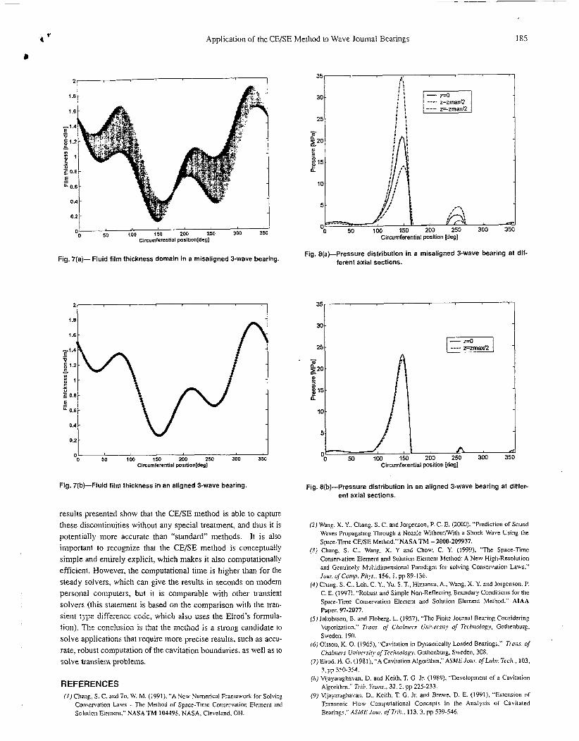
alignment d, that represents the proportion of the actual misalignment to the mraximum possible. i h e maximum misaiignment is restricted by the condition that at the bearing ends (in the axial direction) the film thickness reaches the value of zero. The physical conditions of the bearing are presented in Table 3. Because of the misalignment, the fluid film thickness is a function of both the circumferential and axial coordinates, so that for each value of the circumferential coordinate there is a domain of thickness varia- tion, represented in dark color in Fig. 7(a). Both the aligned and misaligned bearing have the same film thickness distribution at the center plane (which is also the symmetry plane for the aligned case).

Three sections through the pressure distribution, at the mid- plane z = 0, and at mid-distance between this plane and the bearing ends, z = ? L/4, are presented in Fig. 8(a). The maximum calculated pressure is 38.8 MPa (not seen in the figure). The same bearing with identical physical conditions but without misalignment has different values for the pressure distribution, as seen in Fig. 8(b) for the same sections (the pressure distribution i s sym- metric relative to the central plane z = 0. The maximum calculated pressure in this case is 23.2 MPa, at the symmetry plane. The cavitation and the full film regions for the misaligned and the aligned 3-wave bearing are presented respectively in Figs. 9(a), 9(b). The load is found to be 10,523 N for the aligned bearing and 22,115 N for the misaligned bearing, which shows that the misalignment may have a positive impact on bearing performance. This effect is due to the fact that, with misalignment, a region with smaller film thickness is present, compared with the same aligned bearing. This determines the development of higher pressures. At the same time, the region that has a larger film thickness develops cavitation, so that the pressure does not decrease the same amount as it increases in the smaller films thickness region.

CONCLUSIONS

The CE/SE method was applied for the first time to investigate two-dimensional flow in cavitated wave bearings. The theoretical formulation of the solution method was presented along with numerical results. The results were compared with the results obtained using other numerical algorithms. Using Elrod’s formulation, discontinuities can appear at the reformation fronts, and the

Application of the CE/SE Method to Wave Journal Bearings IS5

2 , -

J 50 I 00 150 200 250 300 350

Circumferential poslUon[degl

Fig. 7(a)- Fluid film thickness domain in a misaligned 3-wave bearing.

O2 t OL I

50 100 150 200 250 300 350 ClrcumhrenHal posltion[deg]

Fig. 7(b)-Fluid film thickness in an aligned 3-wave bearing.

results presented show that the CE/SE metliod is able to capture these discontinuities without any special treatment, and thus it is potentially more accurate than “standard” methods. It is also important to recognize that the CE/SE method is conceptually simple and entirely explicit, which makes i t also computationally efficient. However, the computational time is higher than for the steady solvers, which can give the results in seconds on modern personal computers, but it is comparable with other transient solvers (this statement is based on the comparison with the tmi- sip_::! type difference codi, which also uses the Eiroa‘s Eorniuia- ?io!?). The conclusion is that the i i ~ t h o d is a strong candidate to solve applications that require more precise results, such as accurate, robust computation of the cavitation boundaries, as well as to solve transient problenis.

REFERENCES (I) Chang. S. C. and To. W. M. (1991 ), “A New Numerical Framework for Solving

Consc~va~ion Laws - Thc h4ediod of Space-Timc Conser\~alion Elenicn~ and Solution Elenient,” NASA Thl 104495. NASA, Cleveland. OH.

30 -

25

---. z=zmaxl2 /I,“,,, 1 10-

,-, ; .-,‘

200 300

a , a ,

Circumferential position [des]

Fig. 8(a)-Pressure distribution in a misaligned 3-wave bearing at different axial sections.

25

‘0 c 50 100 150 200 250 3W 350

circumferential position [degl

Fig. 8(b)-Pressure distribution in an aligned 3-wave bearing at different axial sections.

(2) Wang. X. Y., Chang. S. C. and Jorgenson, P. C. E. (2000). “Prediction of Sound Waves Propafaling Through a Nozzle Without/With a Shock Wave Using the Space-Time CE/SE Metlrod,”’NASA Thl - 2000-209937.

(3) Chang. S. C.. Wang, X. Y and Chow. C. \’. (1999). “The Spacc-Time Conservation Elemen1 and Solulion Elcinenl Method: A New High-Resolution and Genuinely h~ul~idimensional Paradigm for solving Conservalion Laws.”

(4) Chang, S. C.. Loh. C. Y., Yu. S. T., Himansu, A.. H’ang, X. Y. and Jorgenson. P. C. E. (1997). “Robusl and Simple Non-Reflecting Boundary Conditions for the Space-Time Consen~a~ion el em en^ and Solution Elemenl Method.” AlAA Paper, 97-2077.

(S) Jakobsson. B. and Flokrg. L. ( I 957), “The Finite Journal Bearing Considering Vaponzat~on.” 7i.0,is. of Chahiers Uuiivrsify of S’echrtulogy, Gothenburg, Sweden, 190.

(6) Olsson, K. 0. ( I 965), “Cavitation in Dgnaniically Loaded Bearings,” Trans. of Cliolrners Uf7iiwsit~ of Trchuolugy. Golhenburg, Sweden, 308.

(7) Elrod, H. G. (1981). “A Cavitalion Algorill~m,” ASME Jour. ofLubr. Trch., 103.

[8J Vija)‘araghavan, D. and Keith, T. G. Jr. (1989), develop men^ of a Cavitation Algorithm.“ Fib. Trurts.. 32. 2. pp 225-233.

(91 Vijayaragliavan. D., Keith. T. G. 11.. and Brew, D. E. (1991). “Exlension of Transonic Flow Coniputalional Conceprs in the Analysis of Caviraled Bearings.” ASME ./oiir. of Fib.. 113. 3. pp 539-546.

./Oltr. c7fcO!l l /J . PhJ’S.. 156, 1. 1111 S9-136.

3, pp 350-354.

S. Cioc, E DIMOFTE AND T. KEITH, JR.

circumferential position xl(n 2~ 1

Fig. 9(a)-Cavitation map in a misaligned 3-wave bearing (full film region shown in dark color).

fI0) Cioc, S. and Keith, T. G. (2002) “Application of the CE/SE Method to One- Dimensional Flow in Fluid Film Bearings,” nib. T,.ans.. 45, 2 , pp 169- 176.

( / I ) Chang, S. c., et al. (1998). “Fundamentals of W S E Method,” NASA TM- 1998-208843, NASA, Cleveland, Ohio.

( 1 2 ) Liu, N. S. and Chen, K. H. (2001). “An Alternative Flow Solver for the NCC - the FLUX Code and its Algorithm,’’ AIAA Paper 2001-0973.

(13) Tannehill, J. C., Anderson, D. A. and Pletcher, R. H. (1999). Comprrradond Fluid Mechanics and Heal Transfer, Second Edition, Taylor and Francis, pp 84- 91, 177-274.

__ 0.5

. .- 0.6

Circumferential position xl(n

1 i -

0.8 0.9 1

Fig. S(b)-Cavitation map in an aligned 3-wave bearing (full film region shown in dark color).

(14) Vijayaraghavan, D. (IOSO), “New Concepts in Numerical Prediction of Cavitation in Bearings,” Ph.D. Dissertation, The University of Toledo.

(15) Dimofte, F., Proctor, M. P. and Keith, T. G. (2000), “Wave Fluid Film Bearing Tests for an Aviation Gearbox,’’ NASA TM-2000-209766, NASA, Cleveland, Ohio.

(16) Yang, D., Yu, S. and Zhao, J. (2OOl), “Convergence and Error Bound Analysis for the Space-Time CESE Method,” Numer. Merhods Pnrtid Differential Eq. . 17, pp 64-78.

investigation of pressurized wave bearings

Documents