hydraulics of pressurized flow

8/8/2019 Hydraulics of Pressurized Flow

http://slidepdf.com/reader/full/hydraulics-of-pressurized-flow 1/43

2.1 INTRODUCTION

The need to provide water to satisfy basic physical and domestic needs; use of mar-itime and fluvial routes for transportation and travel, crop irrigation, flood protec-tion, development of stream power; all have forced humanity to face water from thebeginning of time. It has not been an easy rapport. City dwellers who day after daysee water flowing from faucet’s, docile to their needs, have no idea of its idiosyn-

crasy. They cannot imagine how much patience and cleverness are needed to han-dle our great friend-enemy; how much insight must be gained in understanding itsarrogant nature in order to tame and subjugate it; how water must be “enticed” toagree to our will, respecting its own at the same time. That is why a hydraulicianmust first be something like a water psychologist, thoroughly knowledgeable of itsnature. (Enzo Levi, The Science of Water: The Foundations of Modern Hydraulics,ASCE, 1995, p. xiii.)

Understanding the hydraulics of pipeline systems is essential to the rational design,analysis, implementation, and operation of many water resource projects. This chapterconsiders the physical and computational bases of hydraulic calculations in pressurized

pipelines, whether the pipelines are applied to hydroelectric, water supply, or wastewatersystems. The term pressurized pipeline means a pipe system in which a free water surfaceis almost never found within the conduit itself. Making this definition more precise is dif-ficult because even in a pressurized pipe system, free surfaces are present within reser-voirs and tanks and sometimes —for short intervals of time during transient (i.e.,unsteady) events—can occur within the pipeline itself. However, in a pressurized pipelinesystem, in contrast to the open-channel systems discussed in Chapter 3, the pressureswithin the conveyance system are usually well above atmospheric.

Of central importance to a pressurized pipeline system is its hydraulic capacity: that is,its ability to pass a design flow. A related issue is the problem of flow control: how design

flows are established, modified, or adjusted. To deal adequately with thesetwo topics, this chapter considers head-loss calculations in some detail and introduces thetopics of pumping, flow in networks, and unsteady flows. Many of these subjects are treat-ed in greater detail in later chapters, or in reference such as Chaudhry and Yevjevich (1981).

Rather than simply providing the key equations and long tabulations of standardvalues, this chapter seeks to provide a context and a basis for hydraulic design. In addi-tion to the relations discussed, such issues as why certain relations rather than others areused, what various equations assume, and what can go wrong if a relation is used incor-

CHAPTER 2

HYDRAULICS OFPRESSURIZED FLOW

Bryan W. Karney Department of Civil Engineering

University of Toronto,

Toronto, Ontario,

Canada

2.1

Downloaded from Digital Engineering Library @ McGraw-Hill (www.digitalengineeringlibrary.com)Copyright © 2004 The McGraw-Hill Companies. All rights reserved.

Any use is subject to the Terms of Use as given at the website.

Source: HYDRAULIC DESIGN HANDBOOK



rectly also are considered. Although derivations are not provided, some emphasis is placedon understanding both the strengths and weaknesses of various approaches. Given thevirtually infinite combinations and arrangements of pipe systems, such information is

essential for the pipeline professional.

2.2 IMPORTANCE OF PIPELINE SYSTEMS

Over the past several decades, pressurized pipeline systems have become remarkablycompetitive as a means of transporting many materials, including water and wastewater.In fact, pipelines can now be found throughout the world transporting fluids through everyconceivable environment and over every possible terrain.

There are numerous reasons for this increased use. Advances in construction

techniques and manufacturing processes have reduced the cost of pipelines relative toother alternatives. In addition, increases in both population and population density havetended to favor the economies of scale that are often associated with pipeline systems. Theneed for greater conservation of resources and, in particular, the need to limit lossescaused by evaporation and seepage have often made pipelines attractive relative to open-channel conveyance systems. Moreover, an improved understanding of fluid behavior hasincreased the reliability and enhanced the performance of pipeline systems. For all thesereasons, it is now common for long pipelines of large capacity to be built, many of whichcarry fluid under high pressure. Some of these systems are relatively simple, composedonly of series-connected pipes; in others systems, the pipes are joined to form complex

networks having thousands of branched and interconnected lines.Pipelines often form vital links in the process chain, and high penalties may be asso-

ciated with both the direct costs of failure (pipeline repair, cost of lost fluid, damagesassociated with rupture, and so forth) and the interruption of service. This is especiallyevident in industrial applications, such as paper mills, mines, and power plants. Yet, evenin municipal systems, a pipe failure can cause considerable property damage. In addition,the failure may lead indirectly to other kinds of problems. For example, a mainline break could flood a roadway and cause a traffic accident or might make it difficult to fight amajor fire.

Although pipelines appear to promise an economical and continuous supply of fluid,they pose critical problems of design, analysis, maintenance, and operation. A successfuldesign requires the cooperation of hydraulic, structural, construction, survey, geotechni-cal, and mechanical engineers. In addition, designers and planners often must consider thesocial, environmental, and legal implications of pipeline development. This chapter focus-es on the hydraulic considerations, but one should remember that these considerations arenot the only, nor necessarily the most critical, issues facing the pipeline engineer. To besuccessful, a pipeline must be economically and environmentally viable as well as tech-nically sound. Yet, because technical competence is a necessary requirement for any suc-cessful pipeline project, this aspect is the primary focus.

2.3 NUMERICAL MODELS: BASIS FOR PIPELINE ANALYSIS

The designer of a hydraulic system faces many questions. How big should each pipe be tocarry the required flow? How strong must a segment of pipe be to avoid breaking? Arereservoirs, pumps, or other devices required? If so, how big should they be and whereshould they be situated?

2.2 Chapter Two



HYDRAULICS OF PRESSURIZED FLOW



There are at least two general ways of resolving this kind of issue. The first way is tobuild the pipe system on the basis of our “best guess” design and learn about the system’sperformance as we go along. Then, if the original system “as built’’ is inadequate, suc-

cessive adjustments can be made to it until a satisfactory solution is found. Historically, anumber of large pipe systems have been built in more or less this way. For example, theRomans built many impressive water supply systems with little formal knowledge of fluidmechanics. Even today, many small pipeline systems are still constructed with little or noanalysis. The emphasis in this kind of approach should be to design a system that is bothflexible and robust.

However, there is a second approach. Rather than constructing and experimenting withthe real system, a replacement or model of the system is developed first. This model cantake many forms: from a scaled-down version of the original to a set of mathematicalequations. In fact, currently the most common approach is to construct an abstract numer-

ical representation of the original that is encoded in a computer. Once this model is“operational,” experiments are conducted on it to predict the behavior of the real or pro-posed system. If the design is inadequate in any predictable way, the parameters of themodel are changed and the system is retested until design conditions are satisfied. Onlyonce the modeller is reasonably satisfied would the construction of the complete systembe undertaken.

In fact, most modern pipelines systems are modeled quite extensively before they arebuilt. One reason for this is perhaps surprising —experiments performed on a model aresometimes better than those done on the prototype. However, we must be careful here,because better is a relative word. On the plus side, modeling the behavior of a pipelinesystem has a number of intrinsic advantages:

Cost. Constructing and experimenting on the model is often much less expensive thantesting the prototype.

Time. The response rate of the model pipe system may be more rapid and convenientthan the prototype. For example, it may take only a fraction of a second for acomputer program to predict the response of a pipe system after decades of projectedgrowth in the demand for water.

Safety. Experiments on a real system may be dangerous or risky whereas testing themodel generally involves little or no risk.

Ease of modification: Improvements, adjustments, or modifications in design oroperating rules can be incorporated more easily in a model, usually by simply editingan input file.

Aid to communication. Models can facilitate communication between individuals andgroups, thereby identifying points of agreement, disagreement, misunderstanding, orissues requiring clarification.Even simple sketches, such as Fig. 2.1, can aid discussion.

These advantages are often seen as so overwhelming that the fact that alternativeapproaches are available is sometimes forgotten. In particular, we must always rememberthat the model is not reality. In fact, what makes the model useful is precisely its simplic-

ity—it is not as complex or expensive as the original. Stated more forcibly, the model isuseful because it is wrong. Clearly, the model must be sufficiently accurate for its intend-ed purpose or its predictions will be useless. However, the fact that predictions are imper-fect should be no surprise.

As a general rule, systems that are large, expensive, complex, and important justifymore complex and expensive models. Similarly, as the sophistication of the pipeline sys-tem increases, so do the benefits and advantages of the modeling approach because this

Hydraulics of Pressurized Flow 2.3






strategy allows us to consider the consequences of certain possibilities (decisions, actions,inactions, events, and so on before they occur and to control conditions in ways that maybe impossible in practice (e.g., weather characteristics, interest rates, future demands,control system failures). Models often help to improve our understanding of causeand effect and to isolate particular features of interest or concern and are our primary toolof prediction.

To be more specific, two kinds of computer models are frequently constructed forpipeline systems planning models and operational model:

Planning models. These models are used to assess performance, quantity or econom-ic impacts of proposed pipe systems, changes in operating procedures, role of devices,control valves, storage tanks, and so forth. The emphasis is often on selection, sizing, ormodification of devices.

Operational models. These models are used to forecast behavior, adjust pressures orflows, modify fluid levels, train operators, and so on over relatively short periods (hours,days, months). The goal is to aid operational decisions.

The basis of both kinds of models is discussed in this chapter. However, before you

believe the numbers or graphs produced by a computer program, or before you work through the remainder of this chapter, bear in mind that every model is in some sense a fake— it is a replacement, a stand-in, a surrogate, or a deputy for something else. Modelsare always more or less wrong. Yet it is their simultaneous possession of the characteris-tics of both simplicity and accuracy that makes them powerful.

2.4 MODELING APPROACH

If we accept that we are going to construct computer models to predict the performance

of pipeline systems, then how should this be done? What aspects of the prototype can andshould be emphasized in the model? What is the basis of the approximations, and whatprinciples constrain the approach? These topics are discussed in this section.

Perhaps surprisingly, if we wish to model the behavior of any physical system, aremarkably small number of fundamental relations are available (or required). In essence,we seek to answer three simple questions: where?, what? and how? The following sectionsprovide elaboration.

2.4 Chapter Two

FIGURE 2.1Energy relations in a simple pipe system.

∆ H

EGL1

EGL2

Valve






The first question is resolved most easily. Because flow in a pipe system can almostalways be assumed to be one-dimensional, the question of where is resolved by assuminga direction of flow in each link of pipe. This assumed direction gives a unique orientation

to the specification of distance, discharge, and velocity. Positive values of these variablesindicate flow in the assumed direction, whereas negative values indicate reverse flows.The issues of what and how require more careful development.

2.4.1 Properties of Matter (What?)

The question of ‘What?’ directs our attention to the matter within the control system. Inthe case of a hydraulic system, this is the material that makes up the pipe walls, or fills theinterior of a pipe or reservoir, or that flows through a pump. Eventually a modeller must

account for all these issues, but we start with the matter that flows, typically consistingmostly of water with various degrees of impurities.

In fact, water is so much a part of our lives that we seldom question its role. Yet waterpossesses a unique combination of chemical, physical, and thermal properties that makesit ideally suited for many purposes. In addition, although important regional shortagesmay exist, water is found in large quantities on the surface of the earth. For both these rea-sons, water plays a central role in both human activity and natural processes.

One surprising feature of the water molecule is its simplicity, formed as it as from twodiatomic gases, hydrogen (H2) and oxygen (O2). Yet the range and variety of water’sproperties are remarkable (Table 2.1 provides a partial list). Some property values in the

Hydraulics of pressurized flow 2.5

TABLE 2.1 Selected Properties of Liquid Water

Physical Properties

1. High density— liq < 1 000 kg/m3

2. Density maximum at 4ºC—i.e., above freezing!

3. High viscosity (but a Newtonian fluid)— ≈ 10–3

N · s/m2

4. High surface tension— ≈ 73 N/m

5. High bulk modulus (usually assumed incompressible)—K ≈ 2.07 GPa

Thermal Properties1. Specific Heat—highest except for NH3—c ≈ 4.187 kJ/(kg·ºC)

2. High heat of vaporization—cv ≈ 2.45 MJ/kg

3. High heat of fusion—c f ≈ 0.36 MJ/kg

4. Expands on freezing—in almost all other compounds, solid > liq

5. High boiling point—c.f., H2 (20 K), O2 (90 K) and H2O (373 K)

6 Good conductor of heat relative to other liquids and nonmetal solids.

Chemical and Other Properties

1. Slightly ionized—water is a good solvent for electrolytes and nonelectrolytes

2. Transparent to visible light; opaque to near infrared

3. High dielectric constant—responds to microwaves and electromagnetic fields

Note: The values are approximate. All the properties listed are functions of temperature, pressure, water purity, andother factors that should be known if more exact values are to be assigned. For example, surface tension is greatly

influenced by the presence of soap films, and the boiling point depends on water purity and confining pressure. Thevalues are generally indicative of conditions near 10ºC and one atmosphere of pressure.






table —especially density and viscosity values—are used regularly by pipeline engineers.Other properties, such as compressibility and thermal values, are used indirectly, primar-ily to justify modeling assumptions, such as the flow being isothermal and incompress-

ible. Many properties of water depend on intermolecular forces that create powerfulattractions (cohesion) between water molecules. That is, although a water molecule iselectrically neutral, the two hydrogen atoms are positioned to create a tetrahedral chargedistribution on the water molecule, allowing water molecules to be held strongly togetherwith the aid of electrostatic attractions. These strong internal forces—technically called‘hydrogen bonds’—arise directly from the non-symmetrical distribution of charge.

The chemical behavior of water also is unusual. Water molecules are slightly ionized,making water an excellent solvent for both electrolytes and nonelectrolytes. In fact, wateris nearly a universal solvent, able to wear away mountains, transport solutes, and supportthe biochemistry of life. But the same properties that create so many benefits also create

problems, many of which must be faced by the pipeline engineer. Toxic chemicals, disin-fection byproducts, aggressive and corrosive compounds, and many other substances canbe carried by water in a pipeline, possibly causing damage to the pipe and placing con-sumers at risk.

Other challenges also arise. Water’s almost unique property of expanding on freezingcan easily burst pipes. As a result, the pipeline engineer either may have to bury a line ormay need to supply expensive heat-tracing systems on lines exposed to freezing weather,particularly if there is a risk that standing water may sometimes occur. Water’s high vis-cosity is a direct cause of large friction losses and high energy costs whereas its vaporproperties can create cavitation problems in pumps, valves, and pipes. Furthermore, thecombination of its high density and small compressibility creates potentially dramatictransient conditions. We return to these important issues after considering how pipelineflows respond to various physical constraints and influences in the next section.

2.4.2 Laws of Conservation (How?)

Although the implications of the characteristics of water are enormous, no mere list of itsproperties will describe a physical problem completely. Whether we are concerned withwater quality in a reservoir or with transient conditions in a pipe, natural phenomena alsoobey a set of physical laws that contributes to the character and nature of a system’s

response. If engineers are to make quantitative predictions, they must first understand thephysical problem and the mathematical laws that model its behavior.

Basic physical laws must be understood and be applied to a wide variety of applica-tions and in a great many different environments: from flow through a pump to transientconditions in a channel or pipeline. The derivations of these equations are not provided,however, because they are widely available and take considerable time and effort to doproperly. Instead, the laws are presented, summarized, and discussed in the pipeline con-text. More precisely, a quantitative description of fluid behavior requires the applicationof three essential relations: (1) a kinematic relation obtained from the law of mass con-servation in a control volume, (2) equations of motion provided by both Newton’s second

law and the energy equation, and (3) an equation of state adapted from compressibilityconsiderations, leading to a wavespeed relation in transient flow and justifying theassumption of an incompressible fluid in most steady flow applications.

A few key facts about mass conservation and Newton’s second law are reviewedbriefly in the next section. Consideration of the energy equation is deferred until steadyflow is discussed in more detail, whereas further details about the equation of state areintroduced along with considerations of unsteady flow.

2.6 Chapter Two






2.4.3 Conservation of Mass

One of a pipeline engineers most basic, but also most powerful, tools is introduced. in this

section. The central concept is that of conservation of mass a and its key expression is thecontinuity or mass conservation equation.

One remarkable fact about changes in a physical system is that not everything changes.In fact, most physical laws are conservation laws: They are generalized statements aboutregularities that occur in the midst of change. As Ford (1973) said:

A conservation law is a statement of constancy in nature—in particular, constancyduring change. If for an isolated system a quantity can be defined that remainsprecisely constant, regardless of what changes may take place within the system,the quantity is said to be absolutely conserved.

A number of physical quantities have been found that are conserved in the sense of Fords quotation. Examples include energy (if mass is accounted for), momentum, charge,and angular momentum. One especially important generalization of the law of mass con-servation includes both nuclear and chemical reactions (Hatsopoulos and Keenan, 1965).

2.4.3.1 Law of Conservation of Chemical Species “ Molecular species are conserved inthe absence of chemical reactions and atomic species are conserved in the absence of nuclear reactions”. In essence, the statement is nothing more a principle of accounting,stating that number of atoms or molecules that existed before a given change is equal tothe number that exists after the change. More powerfully, the principle can be transformed

into a statement of revenue and expenditure of some commodity over a definite period of time. Because both hydraulics and hydrology are concerned with tracking the distributionand movement of the earth’s water, which is nothing more than a particular molecularspecies, it is not surprising that formalized statements of this law are used frequently.These formalized statements are often called water budgets, typically if they apply to anarea of land, or continuity relations, if they apply in a well-defined region of flow (theregion is well–defined; the flow need not be).

The principle of a budget or continuity equation is applied every time we balance acheckbook. The account balance at the end of any period is equal to the initial balance plus

all the deposits minus all the withdrawals. In equation form, this can be written as follows:

(balance) f (balance)i ∑ deposits ∑ withdrawals

Before an analogous procedure can be applied to water, the system under considera-tion must be clearly defined. If we return to the checking-account analogy, this require-ment simply says that the deposits and withdrawals included in the equation apply to oneaccount or to a well-defined set of accounts. In hydraulics and hydrology, the equivalentrequirement is to define a control volume—a region that is fixed in space, completely sur-rounded by a “control surface,” through which matter can pass freely. Only when the

region has been precisely defined can the inputs (deposits) and outputs (withdrawals) beidentified unambiguously.If changes or adjustments in the water balance (∆S) are the concern, the budget con-

cept can be expressed as

∆S S f Si (balance) f (balance)i V i V o (2.1)







where V i represents the sum of all the water entering an area, and V o indicates the total vol-ume of water leaving the same region. More commonly, however, a budget relation suchas Eq. 2.1 is written as a rate equation. Dividing the “balance’’ equation by ∆t and

taking the limit as ∆t goes to zero produces

S’

d d St I O (2.2)

where the derivative term S’ is the time rate of change in storage, S is the water stored inthe control volume, I is the rate of which water enters the system (inflow), and O is therate of outflow. This equation can be applied in any consistent volumetric units (e.g., m3 /s,ft3 /s, L/s, ML/day, etc.)

When the concept of conservation of mass is applied to a system with flow, such as apipeline, it requires that the net amount of fluid flowing into the pipe must be accounted

for as fluid storage within the pipe. Any mass imbalance (or, in other words, net massexchange) will result in large pressure changes in the conduit because of compressibilityeffects.

2.4.3.2 Steady Flow Assuming, in addition, that the flow is steady, Eq. 2.2 can bereduced further to inflow = outflow or I = O. Since the inflow and outflow may occur atseveral points, this is sometimes re-written as

inflow

V i Ai outflow

V i Ai (2.3)

Equation (2.3) states that the rate of flow into a control volume is equal to the rate of outflow. This result is intuitively satisfying since no accumulation of mass or volumeshould occur in any control volume under steady conditions. If the control volume weretaken to be the junction of a number of pipes, this law would take the form of Kirchhoff’scurrent law—the sum of the mass flow in all pipes entering the junction equals the sum of the mass flow of the fluid leaving the junction. For example, in Fig. 2.2, continuity for thecontrol volume of the junction states that

Q1 Q2 Q3 Q4 (2.4)

2.4.4 Newton’s Second Law

When mass rates of flow are concerned, the focus is on a single component of chemicalspecies. However, when we introduce a physical law, such as Newton’s law of motion, weobtain something even more profound: a relationship between the apparently unrelatedquantities of force and acceleration.

More specifically, Newton’s second law relates the changes in motion of a fluid orsolid to the forces that cause the change. Thus, the statement that the resultant of all exter-nal forces, including body forces, acting on a system is equal to the rate of change of

momentum of this system with respect to time. Mathematically, this is expressed as

F ext = (2.5)

where t is the time and F ext represents the external forces acting on a body of mass mmoving with velocity υ. If the mass of the body is constant, Eq. (2.5) becomes

d (mv)

dt

2.8 Chapter Two






F ext = m

d d vt ma (2.6)

where a is the acceleration of the system (the time rate of change of velocity).

In closed conduits, the primary forces of concern are the result of hydrostatic pressure,fluid weight, and friction. These forces act at each section of the pipe to produce the netacceleration. If these forces and the fluid motion are modeled mathematically, the resultis a “dynamic relation” describing the transient response of the pipeline.

For a control volume, if flow properties at a given position are unchanging with time,the steady form of the moment equation can be written as

F ext = 0cs

ρv(v n) dA (2.7)

where the force term is the net external force acting on the control volume and the right

hand term gives the net flux of momentum through the control surface. The integral istaken over the entire surface of the control volume, and the integrand is the incrementalamount of momentum leaving the control volume.

The control surface usually can be oriented to be perpendicular to the flow, and onecan assume that the flow is incompressible and uniform. With this assumption, themomentum equation can be simplified further as follows:

F ext = (ρ A v)out (ρ A v)in ρQ(vout vin) (2.8)

where Q is the volumetric rate of flow.

Example: Forces at an Elbow. One direct application of the momentum relation isshown in Fig. 2.3, which indicates the flows and forces at elbow. The elbow is assumed tobe mounted in a horizontal plane so that the weight is balanced by vertical forces (notshown).


Q1

Q2

Q3

Q4

CV

FIGURE 2.2 Continuity at a pipe junction Q1 + Q2 = Q3 + Q4






The reaction forces shown in the diagram are required for equilibrium if the elbow isto remain stationary. Specifically, the force F x must resist both the pressure force and mustaccount for the momentum-flux term. That is, taking x as positive to the right, direct appli-cation of the momentum equation gives

(PA)1 F x ρQ 1 (2.9)

Thus,

F x (PA)1 ρQ 1 (2.10)

In a similar manner, but taking y as positive upward, direct application of the momen-tum equation gives

(PA)2 F y ρQ( 2) (2.11)

(here the outflow gives a positive sign, but the velocity is in the negative direction). Thus,F y (PA)2 + ρQ 2 (2.12)

In both cases, the reaction forces are increased above what they would be in the sta-tic case because the associated momentum must either be established or be eliminatedin the direction shown. Application of this kind of analysis is routine in designing thrustblocks, which are a kind of anchor used at elbows or bends to restrain the movement of pipelines.

2.5 SYSTEM CAPACITY: PROBLEMS IN TIME AND SPACE

A water transmission or supply pipeline is not just an enclosed tube— it is an entire sys-tem that transports water, either by using gravity or with the aid of pumping, from itssource to the general vicinity of the demand. It typically consists of pipes or channels withtheir associated control works, pumps, valves, and other components. A transmission sys-

2.10 Chapter Two

(PA )1

F x

F y

y

x

CV

(PA )2

V 1

V 2

FIGURE 2.3 Force and momentum fluxes at an elbow.






tem is usually composed of a single-series line, as opposed to a distribution system thatoften consists of a complex network of interconnected pipes.

As we have mentioned, there are many practical questions facing the designer of such

a system. Do the pipes, reservoirs and pumps have a great enough hydraulic capacity? Canthe flow be controlled to achieve the desired hydraulic conditions? Can the system beoperated economically? Are the pipes and connections strong enough to withstand bothunsteady and steady pressures?

Interestingly, different classes of models are used to answer them, depending on thenature of the flow and the approximations that are justified. More specifically, issues of hydraulic capacity are usually answered by projecting demands (water requirements) andanalyzing the system under steady flow conditions. Here, one uses the best available esti-mates of future demands to size and select the primary pipes in the system. It is thehydraulic capacity of the system, largely determined by the effective diameter of the

pipeline, that links the supply to the demand.Questions about the operation and sizing of pumps and reservoirs are answered by

considering the gradual variation of demand over relatively short periods, such as over anaverage day or a maximum day. In such cases, the acceleration of the fluid is often negli-gible and analysts use a quasi-steady approach: that is, they calculate forces and energybalances on the basis of steady flow, but the unsteady form is used for the continuity equa-tion so that flows can be accumulated and stored.

Finally, the issue of required strength, such as the pressure rating of pipes and fittings,is answered by considering transient conditions. Thus, the strength of a pipeline is deter-mined at least in part by the pressures generated by a rapid transition between flow states.In this stage, short-term and rapid motions must be taken into account, because largeforces and dangerous pressures can sometimes be generated. Here, forces are balancedwith accelerations, mass flow rates with pressure changes. These transient conditions arediscussed in more detail in section 2.8 and in chapter 10.

A large number of different flow conditions are encountered in pipeline systems. Tofacilitate analysis, these conditions are often classified according to several criteria. Flowclassification can be based on channel geometry, material properties, dynamic consider-ations (both kinematic and kinetic), or some other characteristic feature of the flow. Forexample, on the basis of fluid type and channel geometry, the flow can be classified asopen-channel, pressure, or gas flow. Probably the most important distinctions are basedon the dynamics of flow (i.e., hydraulics). In this way, flow is classified as steady or

unsteady, turbulent or laminar, uniform or nonuniform, compressible or incompressible,or single phase or multiphase. All these distinctions are vitally important to the analyst:collectively, they determine which physical laws and material properties are dominant inany application.

Steady flow: A flow is said to be steady if conditions at a point do not change withtime. Otherwise a flow is unsteady or transient . By this definition, all turbulent flows, andhence most flows of engineering importance, are technically unsteady. For this reason, amore restrictive definition is usually applied: A flow is considered steady if the temporalmean velocity does not change over brief periods. Although the assumption is not for-mally required, pipeline flows are usually considered to be steady; thus, transient condi-tions represent an ‘abnormal’, or nonequilibrium, transition from one steady-state flow toanother. Unless otherwise stated, the initial conditions in transient problems are usuallyassumed to be steady.

Steady or equilibrium conditions in a pipe system imply a balance between the physi-cal laws. Equilibrium is typified by steady uniform flow in both open channels and closedconduits. In these applications, the rate of fluid inflow to each segment equals the rate of







outflow, the external forces acting on the flow are balanced by the changes in momentum,and the external work is compensated for by losses of mechanical energy. As a result, thefluid generally moves down an energy gradient, often visualized as flow in the direction

of decreasing hydraulic grade-line elevations (e.g., Fig. 2.1).Quasi-steady flow. When the flow becomes unsteady, the resulting model that must

be used depends on how fast the changes occur. When the rate of change is particular-ly slow, typically over a period of hours or days, the rate of the fluids acceleration isnegligible. However, fluid will accumulate or be depleted at reservoirs, and rates of demand for water may slowly adjust. This allows the use of a quasi-steady or extend-ed-duration simulation model.

Compressible and Incompressible. If the density of the fluid is constant—both intime and throughout the flow field—a flow is said to be incompressible. Thus, is not afunction of position or time in an incompressible flow. If changes in density are permitted

or reguined the flow is compressible.

Surge. When the rate of change in flow is moderate, typically occurring over a periodof minutes, a surge model is often used. In North America, the term surge indicates ananalysis of unsteady flow conditions in pipelines when the following assumptions aremade: the fluid is incompressible (thus, its density is constant) and the pipe walls are rigidand do not deform. These two assumptions imply that fluid velocities are not a functionof position along a pipe of constant cross-section and the flow is uniform. In other words,no additional fluid is stored in a length of pipe as the pressure changes; because velocitiesare uniform, the rate at which fluid enters a pipe is always equal to the rate of discharge.However, the acceleration of the fluid and its accumulation and depletion from reservoirs

are accounted for in a surge model.

Waterhammer. When rapid unsteady flow occurs in a closed conduit system, the tran-sient condition is sometimes marked by a pinging or hammering noise, appropriatelycalled waterhammer . However, it is common to refer to all rapidly changing flow condi-tions by this term, even if no audible shock waves are produced. In waterhammer models,it is usually assumed that the fluid is slightly compressible, and the pipe walls deform withchanges in the internal pressure. Waterhammer waves propagate with a finite speed equalto the velocity of sound in the pipeline.

The speed at which a disturbance is assumed to propagate is the primary distinction

between a surge and a waterhammer model. Because the wavespeed parameter a is relat-ed to fluid storage, the wavespeed is infinite in surge or quasi-steady models. Thus, ineffect, disturbances are assumed to propagate instantly throughout the pipeline system. Of course they do no such thing, because the wavespeed is a finite physical property of a pipesystem, much like its diameter, wall thickness, or pipeline material. The implication of using the surge or quasi-steady approximation is that the unsteady behavior of the pipesystem is controlled or limited by the rate at which the hydraulic boundary conditions(e.g., pumps, valves, reservoirs) at the ends of the pipe respond to the flow and that thetime required for the pipeline itself to react is negligible by comparison.

Although unsteady or transient analysis is invariably more involved than is steady-state

modeling, neglecting these effects in a pipeline can be troublesome for one of tworeasons: the pipeline may not perform as expected, possibly causing large remedialexpenses, or the line may be overdesigned with respect to transient conditions, possiblycausing unnecessarily large capital costs. Thus, it is essential for engineers to have a clearphysical grasp of transient behavior and an ability to use the computer’s power to maxi-mum advantage.

One interesting point is that as long as one is prepared to assume the flow is com-pressible, the importance of compressibility does not need to be known a priory. In fact,

2.12 Chapter Two






all the incompressible, quasi-steady, and steady equations are special cases of the full tran-sient equations. Thus, if the importance of compressibility or acceleration effects isunknown, the simulation can correctly assume compressible flow behavior and allow the

analysis to verify or contradict this assumption.Redistribution of water, whatever model or physical devices are used, requires control

of the fluid and its forces, and control requires an understanding not only of physical lawbut also of material properties and their implications. Thus, an attempt to be more specif-ic and quantitative about these matters will be made as this chapter progresses.

In steady flow, the fluid generally moves in the direction of decreasing hydraulicgrade-line elevations. Specific devices, such as valves and transitions, cause local pressuredrops and dissipate mechanical energy; operating pumps do work on the fluid and increasedownstream pressures while friction creates head losses more or less uniformly along thepipe length. Be warned, however—in transient applications, this orderly situation rarely

exists. Instead, large and sudden variations of both discharge and pressure can occur andpropagate in the system, greatly complicating analysis.

2.6 STEADY FLOW

The design of steady flow in pipeline systems has two primary objectives. First, thehydraulic objective is to secure the desired pressure and flow rate at specific locations inthe system. Second the economic objective is to meet the hydraulic requirements with theminimum expense.

When a fluid flows in a closed conduit or open channel, it often experiences a com-plex interchange of various forms of mechanical energy. In particular, the work that isassociated with moving the fluid through pressure differences is releted to changes in bothgravitational potential energy and kinetic energy. In addition, the flow may lose mechan-ical energy as a result of friction, a loss that is usually accounted for by extremely smallincreases in the temperature of the flowing fluid (that is, the mechanical energy is con-verted to thermal form).

More specifically, these energy exchanges are often accounted for by using anextended version of Bernoulli’s famous relationship. If energy losses resulting from fric-tion are negligible, the Bernoulli equation takes the following form:

p

γ 1 z1

p

γ 2 z2 (2.13)

where p1 and p2 are the pressures at the end points, γ is the specific weight of the fluid, v1

and v2 are the average velocities at the end points, and z1 and z2 are the elevations of theend points with respect to an arbitrary vertical datum. Because of their direct graphicalrepresentation, various combinations of terms in this relationship are given special labels,historically called heads because of their association with vertical distances. Thus,

Head Definition Associated with

Pressure head p / γ Flow work

Elevation head z Gravitational potential energy

Velocity head v2 /2g Kinetic energy

Piezometric head p / γ z Pressure elevation head

Total head p / γ z v2 /2g Pressure elevation velocity head

v

2

2

2g

v21

2g







A plot of piezometric head along a pipeline forms a line called the hydraulic grade line(HGL). Similarly, a plot of the total head with distance along a pipeline is called the ener-gy grade line (EGL). In the vast majority of municipally related work, velocity heads are

negligible and the EGL and HGL essentially become equivalent.If losses occur, the situation becomes a little more complex. The head loss h f is defined

to be equal to the difference in total head from the beginning of the pipe to the end over atotal distance L. Thus, h f is equal to the product of the slope of the EGL and the pipe length:h f L · S f . When the flow is uniform, the slope of the EGL is parallel to that of the HGL,the difference in piezometric head between the end points of the pipe. Inclusion of a head-loss term into the energy equation gives a useful relationship for describing 1-D pipe flow

p

γ

1 z1

p

γ

2 z2 h f (2.14)

In this relation, the flow is assumed to be from Point 1 to Point 2 and h f is assumed to bepositive. Using capital H to represent the total head, the equation can be rewritten as

H 1 H 2 h f

In essence, a head loss reduces to the total head that would have occurred in the sys-tem if the loss were not present (Fig. 2.1). Since the velocity head term is often small, thetotal head in the above relation is often approximated with the piezometric head.

Understanding head loss is important for designing pipe systems so that they canaccommodate the design discharge. Moreover, head losses have a direct effect on both thepumping capacity and the power consumption of pumps. Consequently, an understandingof head losses is important for the design of economically viable pipe systems.

The occurrence of head loss is explained by considering what happens at the pipe wall,the domain of boundary layer theory. The fundamental assertion of the theory is that whena moving fluid passes over a solid surface, the fluid immediately in contact with the sur-face attains the velocity of the surface (zero from the perspective of the surface). This “noslip” condition gives rise to a velocity gradient in which fluid further from the surface hasa larger (nonzero) velocity relative to the velocity at the surface, thus establishing a shearstress on the fluid. Fluid that is further removed from the solid surface, but is adjacent toslower moving fluid closer to the surface, is itself decelerated because of the fluid’s own

internal cohesion, or viscosity. The shear stress across the pipe section is zero at the cen-ter of the pipe, where the average velocity is greatest, and it increases linearly to a maxi-mum at the pipe wall. The distribution of the shear stress gives rise to a parabolic distrib-ution of velocity when the flow is laminar.

More frequently, the flow in a conduit is turbulent. Because turbulence introduces acomplex, random component into the flow, a precise quantitative description of turbulentflow is impossible. Irregularities in the pipe wall lead to the formation of eddy currentsthat transfer momentum between faster and slower moving fluid, thus dissipating mechan-ical energy. These random motions of fluid increase as the mean velocity increases. Thus,in addition to the shear stress that exists for laminar flow, an apparent shear stress existsbecause of the exchange of material during turbulent flow.

The flow regime–whether laminar, turbulent, or transitional–is generally classified byreferring to the dimensionless Reynold’s number ( Re). In pipelines, Re is given as

Re VD

µρ (2.15)

where V is the mean velocity of the fluid, D is the pipe diameter, ρ is the fluid density, and

v

2

2

2g

v

2

1

2g

2.14 Chapter Two






µ is the dynamic viscosity. Although the exact values taken to limit the range of Re vary withauthor and application, the different flow regimes are often taken as follows: (1) laminarflow: Re ≤ 2000, (2) transitional flow: 2000 ≤ Re ≤ 4000, and (3) turbulent flow: Re > 4000.

These flow regime have a direct influence on the head loss experienced in a pipeline system.

2.6.1 Turbulent Flow

Consider an experiment in which a sensitive probe is used to measure flow velocity in apipeline carrying a flowing fluid. The probe will certainly record the mean or net compo-nent of velocity in the axial direction of flow. In addition, if the flow in the pipeline is tur-bulent, the probe will record many small and abrupt variations in velocity in all three spa-tial directions. As a result of the turbulent motion, the details of the flow pattern will

change randomly and constantly with time. Even in the simplest possible system–an uni-form pipe carrying water from a constant-elevation upstream reservoir to a downstreamvalve–the detailed structure of the velocity field will be unsteady and exceedingly com-plex. Moreover, the unsteady values of instantaneous velocity will exist even if all exter-nal conditions at both the reservoir and valve are not changing with time. Despite this, themean values of velocity and pressure will be fixed as long as the external conditions donot change. It is in this sense that turbulent flows can be considered to be steady.

The vast majority of flows in engineering are turbulent. Thus, unavoidably, engineersmust cope with both the desirable and the undesirable characteristics of turbulence. On thepositive side, turbulent flows produce an efficient transfer of mass, momentum, and ener-gy within the fluid. In fact, the expression to “stir up the pot” is an image of turbulence;it implies a vigorous mixing that breaks up large-scale order and structure in a fluid. Butthe rapid mixing also may create problems for the pipeline engineer. This “down side” caninclude detrimental rates of energy loss, high rates of corrosion, rapid scouring and ero-sion, and excessive noise and vibration as well as other effects.

How does the effective mixing arise within a turbulent fluid? Physically, mixing resultsfrom the random and chaotic fluctuations in velocity that exchange fluid between differ-ent regions in a flow. The sudden, small-scale changes in the instantaneous velocity tendto cause fast moving “packets” of fluid to change places with those of lower velocity andvice verse. In this way, the flow field is constantly bent, folded, and superimposed onitself. As a result, large-scale order and structure within the flow is quickly broken down

and torn apart. But the fluid exchange transports not only momentum but other propertiesassociated with the flow as well. In essence, the rapid and continual interchange of fluidwithin a turbulent flow creates both the blessing and the curse of efficient mixing.

The inherent complexity of turbulent flows introduces many challenges. On one hand,if the velocity variations are ignored by using average or mean values of fluid properties,a degree of uncertainty inevitably arises. Details of the flow process and its variability willbe avoided intentionally, thereby requiring empirical predictions of mean flow character-istics (e.g., head-loss coefficients and friction factors). Yet, if the details of the velocityfield are analyzed, a hopelessly complex set of equations is produced that must be solvedusing a small time step. Such models can rarely be solved even on the fastest computers.

From the engineering view point, the only practical prescription is to accept the empiri-cism necessitated by flow turbulence while being fully aware of its difficulties–the aver-aging process conceals much of what might be important. Ignoring the details of thefluid’s motion can, at times, introduce significant error even to the mean flow calculations.

When conditions within a flow change instantaneously both at a point and in the mean,the flow becomes unsteady in the full sense of the word. For example, the downstreamvalve in a simple pipeline connected to a reservoir might be closed rapidly, creating shock







waves that travel up and down the conduit. The unsteadiness in the mean values of theflow properties introduces additional difficulties into a problem that was already complex.Various procedures of averaging, collecting, and analyzing data that were well justified for

a steady turbulent flow are often questionable in unsteady applications. The entire situa-tion is dynamic: Rapid fluctuations in the average pressure, velocity, and other propertiesmay break or damage the pipe or other equipment. Even in routine applications, specialcare is required to control, predict, and operate systems in which unsteady flows com-monly occur.

The question is one of perspective. The microscopic perspective of turbulence in flowsis bewildering in its complexity; thus, only because the macroscopic behavior is relative-ly predictable can turbulent flows be analyzed. Turbulence both creates the need forapproximate empirical laws and determines the uncertainty associated with using them.The great irregularity associated with turbulent flows tends to be smoothed over both by

the empirical equations and by a great many texts.

2.6.2 Head Loss Caused by Friction

A basic relation used in hydraulic design of a pipeline system is the one describing thedependence of discharge Q (say in m3 /s) on head loss h f (m) caused by friction betweenthe flow of fluid and the pipe wall. This section discusses two of the most commonly usedhead-loss relations: the Darcy-Weisbach and Hazen-Williams equations.

The Darcy-Weisbach equation is used to describe the head loss resulting from flow inpipes in a wide variety of applications. It has the advantage of incorporating a dimen-sionless friction factor that describes the effects of material roughness on the surface of the inside pipe wall and the flow regime on retarding the flow. The Darcy-Weisbach equa-tion can be written as

h f , DW f D

L

2

V

g

2

0.0826 Q

D

2

5Lf (2.16)

where h f , DW = head loss caused by friction (m), f = dimensionless friction factor, L =pipe length (m), D = pipe diameter (m), V = Q / A = mean flow velocity (m/s), Q = dis-charge (m3 /s), A = cross-sectional area of the pipe (m2), and g = acceleration caused bygravity (m/s2).

For noncircular pressure conduits, D is replaced by 4 R, where R is the hydraulic radius.The hydraulic radius is defined as the cross-sectional area divided by the wetted perime-ter or, R = A / P.

Note that the head loss is directly proportional to the length of the conduit and the fric-tion factor. Obviously, the rougher a pipe is and the longer the fluid must travel, the greaterthe energy loss. The equation also relates the pipe diameter inversely to the head loss. Asthe pipe diameter increases, the effects of shear stress at the pipe walls are felt by less of the fluid, indicating that wider pipes may be advantageous if excavation and constructioncosts are not prohibitive. Note in particular that the dependence of the discharge Q on thepipe diameter D is highly nonlinear; this fact has great significance to pipeline designs

because head losses can be reduce dramatically by using a large-diameter pipe, whereasan inappropriately small pipe can restrict flow significantly, rather like a partially closedvalve.

For laminar flow, the friction factor is linearly dependent on the Re with the simplerelationship f = 64/ Re. For turbulent flow, the friction factor is a function of both the Reand the pipes relative roughness. The relative roughness is the ratio of equivalent uniformsand grain size and the pipe diameter (e / D), as based on the work of Nikuradse (1933), who

2.16 Chapter Two






experimentally measured the resistance to flow posed by various pipes with uniform sandgrains glued onto the inside walls. Although the commercial pipes have some degree of spa-tial variance in the characteristics of their roughness, they may have the same resistance char-

acteristics as do pipes with a uniform distribution of sand grains of size e. Thus, if the veloc-ity of the fluid is known, and hence Re, and the relative roughness is known, the friction fac-tor f can be determined by using the Moody diagram or the Colebrook-White equation.

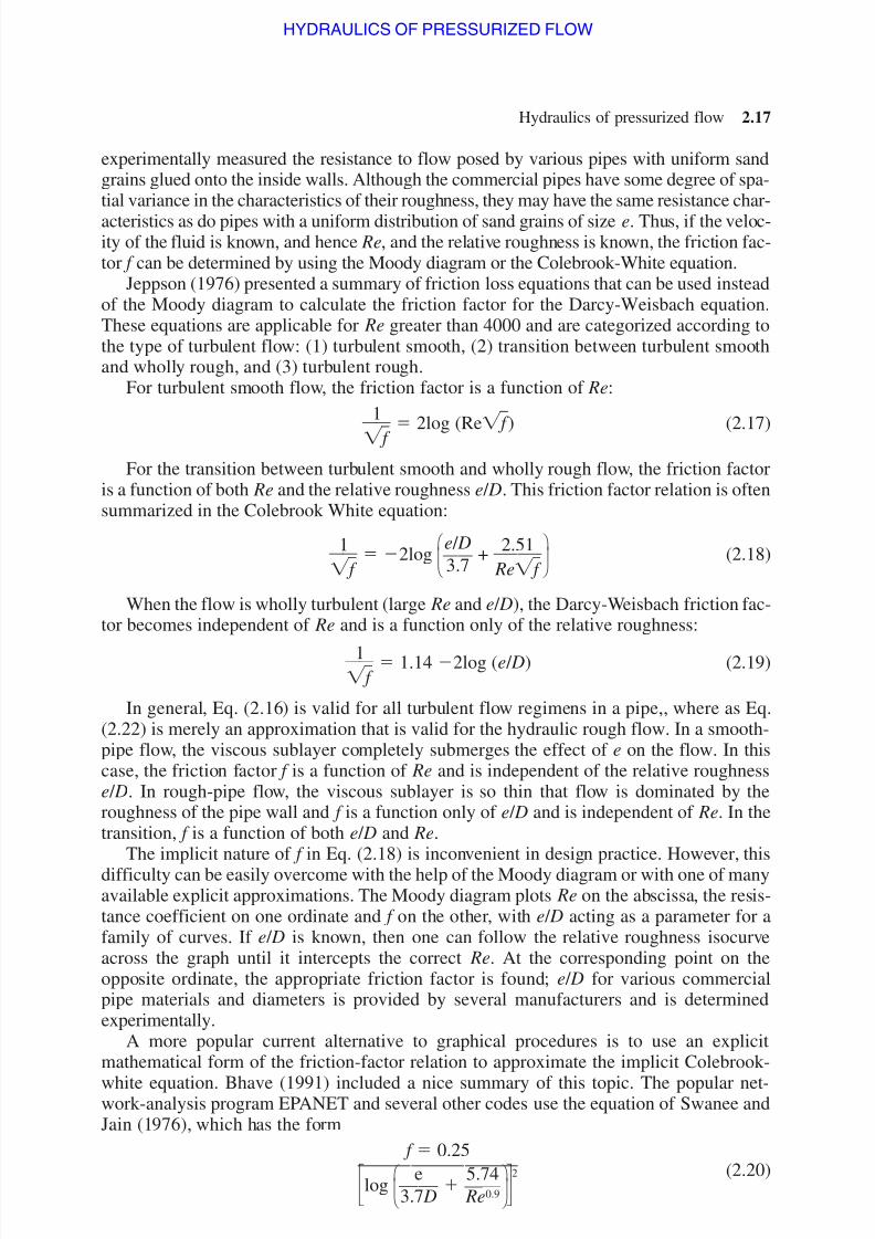
Jeppson (1976) presented a summary of friction loss equations that can be used insteadof the Moody diagram to calculate the friction factor for the Darcy-Weisbach equation.These equations are applicable for Re greater than 4000 and are categorized according tothe type of turbulent flow: (1) turbulent smooth, (2) transition between turbulent smoothand wholly rough, and (3) turbulent rough.

For turbulent smooth flow, the friction factor is a function of Re:

1

f

2log (Re f ) (2.17)

For the transition between turbulent smooth and wholly rough flow, the friction factoris a function of both Re and the relative roughness e / D. This friction factor relation is oftensummarized in the Colebrook White equation:

1

f 2log

e

3

/

.

D

7 +

R

2

e

.

51

f

(2.18)

When the flow is wholly turbulent (large Re and e / D), the Darcy-Weisbach friction fac-tor becomes independent of Re and is a function only of the relative roughness:

1 f 1.14 2log (e / D) (2.19)

In general, Eq. (2.16) is valid for all turbulent flow regimens in a pipe,, where as Eq.(2.22) is merely an approximation that is valid for the hydraulic rough flow. In a smooth-pipe flow, the viscous sublayer completely submerges the effect of e on the flow. In thiscase, the friction factor f is a function of Re and is independent of the relative roughnesse / D. In rough-pipe flow, the viscous sublayer is so thin that flow is dominated by theroughness of the pipe wall and f is a function only of e / D and is independent of Re. In thetransition, f is a function of both e / D and Re.

The implicit nature of f in Eq. (2.18) is inconvenient in design practice. However, this

difficulty can be easily overcome with the help of the Moody diagram or with one of manyavailable explicit approximations. The Moody diagram plots Re on the abscissa, the resis-tance coefficient on one ordinate and f on the other, with e / D acting as a parameter for afamily of curves. If e / D is known, then one can follow the relative roughness isocurveacross the graph until it intercepts the correct Re. At the corresponding point on theopposite ordinate, the appropriate friction factor is found; e / D for various commercialpipe materials and diameters is provided by several manufacturers and is determinedexperimentally.

A more popular current alternative to graphical procedures is to use an explicitmathematical form of the friction-factor relation to approximate the implicit Colebrook-

white equation. Bhave (1991) included a nice summary of this topic. The popular net-work-analysis program EPANET and several other codes use the equation of Swanee andJain (1976), which has the form

(2.20) f 0.25log

3.7

e

D

R

5.

e

70

4.9

2







To circumvent considerations of roughness estimates and Reynolds number depen-dencies, more direct relations are often used. Probably the most widely used of theseempirical head-loss relation is the Hazen-Williams equation, which can be written as

Q C u CD2.63S0.54 (2.21)

where C u unit coefficient (C u 0.314 for English units, 0.278 for metric units), Q

discharge in pipes, gallons/s or m3 /s, L length of pipe, ft or m, d internal diameter of pipe, inches or mm, C Hazen-Williams roughness coefficient, and S = the slope of theenergy line and equals h f / L.

The Hazen-Williams coefficient C is assumed constant and independent of the dis-charge (i.e., R e). Its values range from 140 for smooth straight pipe to 90 or 80 for old,unlined, tuberculated pipe. Values near 100 are typical for average conditions. Values of

the unit coefficient for various combinations of units are summarized in Table 2.2.In Standard International (SI) units, the Hazen-Williams relation can be rewritten forhead loss as

h f,HW 10.654

Q

C

0.154

D

14.87 L (2.22)

where h f,HW is the Hazen-Williams head loss. In fact, the Hazen-Williams equation is notthe only empirical loss relation in common use. Another loss relation, the Manning equa-tion, has found its major application in open channel flow computations. As with the otherexpressions, it incorporates a parameter to describe the roughness of the conduit known

as Manning’s n.Among the most important and surprisingly difficult hydraulic parameter is the diam-

eter of the pipe. As has been mentioned, the exponent of diameter in head-loss equationsis large, thus indicating high sensitivity to its numerical value. For this reason, engineers

2.18 Chapter Two

EGL

H 1 H 2 H 3

(a)

(b)

Q1Q1

Q1

EGL

H 1 H 2

Q2

FIGURE 2.4 Flow in series and parallel pipes.






and analysts must be careful to obtain actual pipe diameters often from manufacturers; the

use of nominal diameters is not recommended. Yet another complication may arise, how-ever. The diameter of a pipe often changes with time, typically as a result of chemicaldepositions on the pipe wall. For old pipes, this reduction in diameter is accounted forindirectly by using an increased value of pipe resistance. Although this approach may bereasonable under some circumstances, it may be a problem under others, especially forunsteady conditions. When ever possible, accurate diameters are recommended for allhydraulic calculations. However, some combinations of pipes (e.g., pipes in series or par-allel; Fig. 2.4) can actualy be represented by a single equivalent diamenter of pipe.

2.6.3 Comparison of Loss Relations

It is generally claimed that the Darcy-Weisbach equation is superior because it is the oret-ically based, where as both the Manning equation and the Hazen-Williams expression useempirically determined resistance coefficients. Although it is true that the functional rela-tionship of the Darcy-Weisbach formula reflects logical associations implied by thedimensions of the various terms, determination of the equivalent uniform sand-grain sizeis essentially experimental. Consequently, the relative roughness parameter used in theMoody diagram or the Colebrook-White equations is not theoretically determined. In thissection, the Darcy-Weisbach and Hazen-Williams equations are compared briefly using asimple pipe as an example.

In the hydraulic rough range, the increase in ∆h f can be explained easily when the ratioof Eq. (2.16) to Eq. (2.22) is investigated. For hydraulically rough flow, Eq. (2.18) can besimplified by neglecting the second term 2.51 ( Re f ) of the logarithmic argument. Thisratio then takes the form of

128.94 1.14 2 log

D

e

2

C

D1

0

.8

.1

5

3

2Q0

1.148 (2.23)

which shows that in most hydraulic rough cases, for the same discharge Q, a larger headloss h f is predicted using Eq. (2.16) than when using Eq. (2.22). Alternatively, for the samehead loss, Eq. (2.22) returns a smaller discharge than does Eq. (2.16).

When comparing head-loss relations for the more general case, a great fuss is oftenmade over unimportant issues. For example, it is common to plot various equations on theMoody diagram and comment on their differences. However, such a comparison is of sec-ondary importance. From a hydraulic perspective, the point is this: Different equationsshould still produce similar similar head discharge behavior. That is, the physical relationbetween head loss and flow for a physical segment of pipe should be predicted well by

h f , HW

h f , DW


TABLE 2.2 Unit Coefficient C u for the Hazen-Williams Equation

Units of Discharge Q Units of Diameter D Unit Coeficient C u

MGD ft 0.279

ft3 /s ft 0.432

GPM in 0.285

GPD in 405

m3 /s m 0.278






2.20 Chapter Two

any practical loss relation. Said even more simply, the issue is how well the h f versus Qcurves compare.

To compare the values of h f determined from Eq. (2.16) and those from Eq. (2.22),

consider a pipe for which the parameters D, L and C are specified. Using the Hazen-Williams relation, it is then possible to calculate h f for a given Q. Then, the Darcy-Weisbach f can be obtained, and with the Colebrook formula Eq. (2.18), the equivalentvalue of roughness e can be found. Finally, the variation of head with discharge can beplotted for a range of flows.

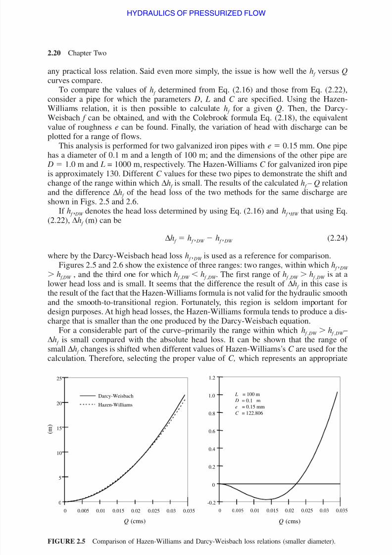
This analysis is performed for two galvanized iron pipes with e 0.15 mm. One pipehas a diameter of 0.1 m and a length of 100 m; and the dimensions of the other pipe are D 1.0 m and L = 1000 m, respectively. The Hazen-Williams C for galvanized iron pipeis approximately 130. Different C values for these two pipes to demonstrate the shift andchange of the range within which ∆h f is small. The results of the calculated h f – Q relation

and the difference ∆h f of the head loss of the two methods for the same discharge areshown in Figs. 2.5 and 2.6.

If h f , DW denotes the head loss determined by using Eq. (2.16) and h f , HW that using Eq.(2.22), ∆h f (m) can be

∆h f h f , DW h f , DW (2.24)

where by the Darcy-Weisbach head loss h f , DW is used as a reference for comparison.Figures 2.5 and 2.6 show the existence of three ranges: two ranges, within which h f , DW

h f,DW , and the third one for which h f ,DW h f ,DW . The first range of h f ,DW h f ,DW is at alower head loss and is small. It seems that the difference the result of ∆h f in this case is

the result of the fact that the Hazen-Williams formula is not valid for the hydraulic smoothand the smooth-to-transitional region. Fortunately, this region is seldom important fordesign purposes. At high head losses, the Hazen-Williams formula tends to produce a dis-charge that is smaller than the one produced by the Darcy-Weisbach equation.

For a considerable part of the curve–primarily the range within which h f ,DW h f ,DW –∆h f is small compared with the absolute head loss. It can be shown that the range of small ∆h f changes is shifted when different values of Hazen-Williams’s C are used for thecalculation. Therefore, selecting the proper value of C, which represents an appropriate

-0.2

0

0.2

0.4

0.6

0.8

1.0

1.2

0 0.005 0.01 0.015 0.02 0.025 0.03 0.035

0

5

10

15

20

25

0 0.005 0.01 0.015 0.02 0.025 0.03 0.035

Q (cms)

L = 100 m

D = 0.1 m

e = 0.15 mm

C = 122.806

Q (cms)

( m )

Hazen-Williams

Darcy-Weisbach

FIGURE 2.5 Comparison of Hazen-Williams and Darcy-Weisbach loss relations (smaller diameter).







point on the head-discharge curve, is essential. If such a C value is used, ∆h f is small, andwhether the Hazen-Williams formula or the Darcy-Weisbach equation is used for thedesign will be of little importance.

This example shows both the strengths and the weaknesses of using Eq. (2.22) as an

approximation to Eq. (2.16). Despite its difficulties, the Hazen-Williams formula is often justified because of its conservative results and its simplicity of use. However, choosing aproper value of either the Hazen-Williams C or the relative roughness e / D is often diffi-cult. In the literature, a range of C values is given for new pipes made of various materi-als. Selecting an appropriate C value for an old pipe is even more difficult. However, if anapproximate value of C or e is used, the difference between the head-loss equations is like-ly to be inconsequential.

Head loss also is a function of time. As pipes age, they are subject to corrosion, espe-cially if they are made of ferrous materials and develop rust on the inside walls, whichincreases their relative roughness. Chemical agents, solid particles, or both in the fluid cangradually degrade the smoothness of the pipe wall. Scaling on the inside of pipes can

occur if the water is hard. In some instances, biological factors have led to time-dependenthead loss. Clams and zebra mussels may grow in some intake pipes and may in some casesdrastically reduce discharge capacities.

2.6.4 Local Losses

Head loss also occurs for reasons other than wall friction. In fact, local losses occur when-ever changes occur in the velocity of the flow: for example, changes in the direction of theconduit, such as at a bend, or changes in the cross-sectional area, such as an aperture,

valve or gauge. The basic arrangement of flow and pressure is illustrated for a venturi con-traction in Fig. 2.7.

The mechanism of head loss in the venturi is typical of many applications involvinglocal losses. As the diagram indicates, there is a section of flow contraction into which theflow accelerates, followed by a section of expansion, into which the flow decelerates.This aspect of the venturi, or a reduced opening at a valve, is nicely described by the con-tinuity equation. However, what happens to the pressure is more interesting and moreimportant.

-1

0

1

2

3

4

5

6

7

8

9

0 2 4 6 8 10

0

20

40

60

80

100

120

0 2 4 6 8 10

Q (cms)

L = 1000 m

D = 1.0 me = 0.15 mm

C = 124.923

Q (cms)

( m )

Hazen-Williams

Darcy-Weisbach

FIGURE 2.6 Comparison of Hazen-Williams and Darcy-Weisbach loss relations (larger diameter).






2.22 Chapter Two

As the flow accelerates, the pressure decreases according to the Bernoulli relation.Everything goes smoothly in this case because the pressure drop and the flow are in thesame direction. However, in the expansion section, the pressure increases in thedownstream direction. To see why this is significant, consider the fluid distributed over thecross section. In the center of the pipe, the fluid velocity is high; the fluid simply slowdown as it moves into the region of greater pressure. But what about the fluid along thewall? Because it has no velocity to draw on, it tends to respond to the increase in pressurein the downstream direction by flowing upstream, counter to the normal direction of flow.That is, the flow tends to separate, which can be prevented only if the faster moving fluidcan “pull it along” using viscosity. If the expansion is too abrupt, this process is not suf-ficient, and the flow will separate, creating a region of recirculating flow within the main

channel. Such a region causes high shear stresses, irregular motion, and large energy loss-es. Thus, from the view point of local losses, nothing about changes in pressure is sym-metrical—adverse pressure gradients or regions of recirculating flow are crucially impor-tant with regard’s to local losses.

Local head losses are often expressed in terms of the velocity head as

hl k 2

v

g

2

(2.25)

where k is a constant derived empirically from testing the head loss of the valve, gauge,and so on, and is generally provided by the manufacturer of the device. Typical forms for

this relation are provided in Table 2.3 (Robertson and Crowe, 1993).

2.6.5 Tractive Force

Fluid resistance also implies a flux in momentum and generates a tractive force, whichraises a number of issues of special significance to the two-phase (liquid-solid) flowsfound in applications of transport of slurry and formation of sludge. In these situations,

1

1 2

EGL

HGLV2

2g

∆h f

EGL

HGL

FIGURE 2.7 Pressure relations in a venturí contraction.






the tractive force has an important influence on design velocities: The velocity cannot betoo small or the tractive force will be insufficient to carry suspended sediment and depo-sition will occur. Similarly, if design velocities are too large, the greater tractive force willincrease rates of erosion and corrosion in the channel or pipeline, thus raising maintenanceand operational costs. Thus, the general significance of tractive force relates to designing


TABLE 2.3 Local Loss Coefficients at Transitions

Additional

Description Sketch Data K Sourcer/d Ke (1)

Pipe entrance 0.0 0.50

0.1 0.12

h L K eV 2 /2g 0.2 0.03

Contraction K c K cD2 /D1 0 5 60º 0 5 180º (1)

0.0 0.08 0.50

0.20 0.08 0.49

0.40 0.07 0.42

0.60 0.06 0.320.80 0.05 0.18

h L K eV 22 /2g 0.90 0.04 0.10

Expansion K E K E

D1 /D2 0 5 10º 0 5 180º (1)

0.0 1.00

0.20 0.13 0.92

0.40 0.11 0.72

0.60 0.06 0.42

h L K E V 21 /2g 0.80 0.03 0.16

Without K b 1.1 (26)90º miter vanes

bendWith K b 0.2 (26)

vanes

90º miter r / d (3)bend 1 K b 0.35 and

2 0.19 (13)

4 0.16

6 0.21

8 0.2810 0.32

Globe valve—wide open K v 10.0 (26)

Threaded Angle valve—wide open K v 5.0

pipe Gate valve—wide open K v 0.2

fittings Gatevalve—half open K v 5.6

Return bend K b 2.2

Tee K t 1.8

90º elbow K b 0.9

45º elbow K b 0.4






self-cleansing channel and pressure-flow systems and to stable channel design in erodiblechannels. Moreover, high tractive forces are capable of causing water quality problems indistribution system piping through the mechanism of biofilm sloughing or suspension of

corrosion by-products.

2.6.6 Conveyance System Calculations: Steady Uniform Flow

A key practical concern in the detailed calculation of pressure flow and the estimation of pressure losses. Because the practice of engineering requires competent execution in ahuge number of contexts, the engineer will encounter many different applications in prac-tice. compare, for example Fig. 2.4 to 2.8 In fact, the number of applied topics is so largethat comprehensive treatment is impossible. Therefore, this chapter emphasizes a system-

atic presentation of the principles and procedures of problem-solving to encourage theengineer’s ability to generalize. To illustrate the principles of hydraulic analysis, this sec-tion includes an example that demonstrates both the application of the energy equationand the use of the most common head-oss equations. A secondary objective is to justifytwo common assumptions about pipeline flow: namely, that flow is, to a good approxi-mation, incompressible and isothermal.

Problem. A straight pipe is 2500 m long 27 inches in diameter and discharges waterat 10ºC into the atmosphere at the rate of 1.80 m3/s. The lower end of the pipe is at an ele-vation of 100 m, where a pressure gauge reads 3.0 MPa. The pipe is on a 4% slope.

1. Determine the pressure head, elevation head, total head, and piezometric level atboth ends of this pipeline.

2. Determine the associated Darcy-Weisbach friction factor f and Hazen-Williams C for this pipeline and flow.

3. Use the known pressure change to estimate the change in density between theupstream and downstream ends of the conduit. Also estimate the associated change

2.24 Chapter Two

FIGURE 2.8 Flow in a simple pipe network.

A

B

190.0 m

C

12

3

D

196.7 m

162.6 m






in velocity between the two ends of the pipe, assuming a constant internal diame-ter of 27 in throughout. What do you conclude from this calculation?

4. Estimate the change in temperature associated with this head loss and flow, assum-ing that all the friction losses in the pipe are converted to an increase in the tem-perature of the water. What do you conclude from this calculation?

Solution. The initial assumption in this problem is that both the density of the waterand its temperature are constant. We confirm at the end of the problem that these are excel-lent assumptions (a procedure similar to the predictor-corrector approaches often used fornumerical methods). We begin with a few preliminary calculations that are common toseveral parts of the problem.

Geometry. If flow is visualized as moving from left to right, then the pipeline is at a100 m elevation at its left end and terminates at an elevation of 100 0.04 (2500) 200m at its right edge, thus gaining 100 m of elevation head along its length. The hydraulicgrade line—representing the distance above the pipe of the pressure head term P / γ —ishigh above the pipe at the left edge and falls linearly to meet the pipe at its right edgebecause the pressure here is atmospheric.

Properties. At 10ºC, the density of water ρ 999.7 kg/m3, its bulk modulus K ρ∆ρ/P/ ∆ρ 2.26 GPa, and its specific heat C 4187 J/(kg · ºC). The weight density isγ ρg 9.81 kN/m3.

Based on an internal diameter of 27 in, or 0.686 m, the cross-sectional area of thepipe is

A

π4 D2

π4 (0.686)2 0.370 m2

Based on a discharge Q 1.80 m3 /s, the average velocity is

V

Q

A

1

0

.

.

8

3

0

70

m

m

3 /s2

4.87 m/s

Such a velocity value is higher than is typically allowed in most municipal work.

1. The velocity head is given by

hv

2vg

2

1.21 m

Thus, the following table can be completed:

Variable Expression Upstream Downstream

Pressure (MPa) P 3.0 0.0

Pressure head (m) P / γ 305.9 0.0

Elevation head (m) z 100.0 200.0

Piezometric head (m) P / γ z 405.9 200.0Total head (m) P / γ z v2 /2g 407.1 201.2

2. The head loss caused by friction is equal to the net decrease in total head over thelength of the line. That is, h f 407.1 201.2 205.9 m. Note that because thispipe is of uniform diameter, this value also could have been obtained from thepiezometric head terms.







From the Darcy-Weisbach equation, we can obtain the following expression for thedimensionless f :

f

(2(20550.90))((01..62816))

0.047

Alternatively, from the Hazen-Williams equation that Q 0.278 C D2.63

(h f / L)0.54, we obtain the following for the dimensional C:

C = 67.2

These values would indicate a pipe in poor condition, probably in much need of repair or replacement.

3. In most problems involving steady flow, we assume that the compressibility of thewater is negligible. This assumption is easily verified since the density change asso-ciated with the pressure change is easily computed.

In the current problem, the pressure change is 3.0 MPa and the bulk modulus is2200 MPa. Thus, by definition of the bulk modulus K,

∆ρρ

∆K

P

22

3

00 0.0014

Clearly, even in this problem, with its unusually extreme pressure changes, the rel-ative change in density is less than 0.2 percent. The density at the higher pressure(upstream) end of the pipe is ρ1 ρ2 ∆ρ 999.7 (1 0.0014) 1001.1 kg/m3.Using the mass continuity equation, we have

ρ( AV )1 (ρ AV )2

In this case, we assume that the pipe is completely rigid and that the change inpressure results in a change in density only (in most applications, these terms arelikely to be almost equally important). In addition, we assume that the velocity

we’ve already calculated applies at the downstream end (i.e., at Location 2). Thus,the continuity equation requires

V 1 V 2 ρρ

2

1

4.871

9

0

9

0

9

1

.7

.1 4.86 m/s

Obviously, even in this case, the velocity and density changes are both negligibleand the assumption of incompressible flow is an extremely good one.

4. Assuming that the flow is incompressible, the energy dissipated, Pd , can be com-puted using work done in moving the fluid through a change in piezometric flow

(in fact, the head loss is nothing more than the energy dissipating per unit rate of weight of fluid transferred). Thus,

Pd γ Qh f

Strictly speaking, this energy is not lost but is transferred to less available forms: typ-ically, heat. Since energy is associated with the increase in temperature of the fluid, we

1.8

0.278(0.686)2.63(205.9/2500)0.54

Q

0.278 D2.63(h f / L)0.54

h f D

L

2

v

g

2

2.26 Chapter Two






can easily estimate the increase in temperature of the fluid that would be associated withthe dissipation of energy, assuming that all the heat is retained in the fluid. That is, P f

ρQ c∆T ρgqhf. Solving for the temperature increase gives

∆T

g

c

h f 0.48ºC.

We conclude that the assumption of isothermal flow also is an excellent one.

2.6.7 Pumps: Adding Energy to the Flow

Although water is the most abundant substance found on the surface of the earth, its nat-

ural distribution seldom satisfies an engineer’s partisan requirements. As a result, pump-ing both water and wastewater is often necessary to achieve the desired distribution of flow. In essence, a pump controls the flow by working on the flowing fluid, primarily bydischarging water to a higher head at its discharge flange than is found at the pump inlet.The increased head is subsequently dissipated as frictional losses within the conduit or isdelivered further downstream. This section provides a brief introduction to how pumpsinteract with pipe systems. Further details are found in Chap. 10.

How exactly is the role of a pump quantified? The key definition is the total dynamichead (TDH) of the pump. This term describes the difference between the total energy on thedischarge side compared with that on the suction side. In effect, the TDH H P is the differencebetween the absolute total head at the discharge and suction nozzle of the pump: that is,

H P h p

2

V

g

2

d

h p

2

V

g

2

s

(2.26)

where h p hydraulic grade line elevation (i.e., pressure-plus-elevation head with respectto a fixed datum), and subscripts d and s refer to delivery and suction flanges, respective-ly. Typically, the concern is how the TDH head varies with the discharge Q; for a pump,this H Q relation is called the characteristic curve.

What the TDH definition accomplishes can be appreciated better if we consider a typ-ical pump system, such as the one shown in Fig. 2.9. In this relation, the Bernoulli equa-tion relates what happens between Points 1 and 2 and between Points 3 and 4, but techni-cally it cannot be applied between 2 and 3 because energy is added to the flow. However,the TDH definition spans this gap.

To see this more clearly, the energy relation is written between Points 1 and 2 as

H S H

PS h fs (2.27)

where H s is the head of the suction reservoir, H PS

is the total head at the suction flange of the pump, and h fs is the friction loss in the suction line. Similarly, the energy relation iswritten between Points 3 and 4 as

H PD

H D

h fd (2.28)

where H d is the head of the discharge reservoir, H PD is the head at the discharge flange of the pump, and h fd is the friction loss in the discharge line. If Eq. (2.27) is then added toEq. (2.28), the result can be rearranged as

H pd H ps H d H s h fd h fs (2.29)

(9.91m/s2)(205.9 m)

4187 J/(kg ·ºC)







which can be rewritten using Eq. (2.26) as

H p H st h f (2.30)

where H st is the total static lift and h f is the total friction loss. The total work done by thepump is equal to the energy required to lift the water from the lower reservoir to the high-er reservoir plus the energy required to overcome friction losses in both the suction anddischarge pipes.

2.6.8 Sample Application Including Pumps

Problem. Two identical pumps are connected in parallel and are used to force water into

the transmission/distribution pipeline system shown in Fig. 2.10. The elevations of thedemand locations and the lengths of C 120 pipe also are indicated. Local losses are neg-ligible in this system and can be ignored. The demands are as follows: D1 1.2 m3 /s, D2 1.6 m3 /s, and D3 = 2.2 m3 /s. The head-discharge curve for a single pump is approx-imated by the equation

H 90 6Q1.70

1. What is the minimum diameter of commercially available pipe required for the 4.2km length if a pressure head is to be maintained at a minimum of 40 m everywhere

in the system? What is the total dynamic head of the pump and the total waterhorsepower supplied for this flow situation?

2. For the system designed in the previous questions the demand can shift as followsunder certain emergency situations: D1 0.8 m3 /s, D2 1.2 m3 /s, and D3 4.2m3 /s. For this new demand distribution, can the system maintain a residual pressurehead of 20 m in the system?

2.28 Chapter Two

HS

HD

HST HP

HPD

HPS

Pump

1

2

4

HGL

3

HGL

FIGURE 2.9 Definition sketch for pump system relations.






Solution. Total flow is Qt D1 D2 D3 1.2 1.6 2.2 5.0 m3 /s and, eachpump will carry half of this flow: i.e., Q pump Qt /2 2.5 m3 /s. The total dynamic headof the pump H pump is

H pump 90 6(2.5)1.7 61.51 m

which allows the total water power to be computed as

Power 2 (Q pump H pumpγ ) Qt H pumpγ

Thus, numerically,

Power 5.0

m

s

3

(61.51m) 9810

m

N 3

3017 kW

which is a huge value. The diameter d 1 of the pipe that is 4.2 km long, the head loss ∆hi

caused by friction for each pipe can be determined using the Hazen-Williams formulasince the flow can be assumed to be in the hydraulic rough range. Because d 1 is unknown,∆h2, ∆h3, and ∆h1 are calculated first. The site where the lowest pressure head occurs canbe shown to be at Node 2 (i.e., the highest node in the system) as follows:

∆h3 L3

0.154

800

0.154

3.80 m

Because the head loss ∆h3 is less than the gain in elevation of 10 m, downstream pres-

sures increase; thus, Node 2 (at D2) will be critical in the sense of having the lowest pres-sure. Thus, if the pressure head at that node is greater than 40 m, a minimum pressure headof 40 m will certainly be maintained throughout the pipeline.

Continuing with the calculations,

∆h2 L2

0.27

Q

8C 2

d 2.63

0.154

1000

0.154

2.30 m3.8

0.278(120)(1.5242.63)

2.2

0.278(120)(1.0672.63)

Q3

0.278Cd 2.63


FIGURE 2.10 Example pipe and pump system.

Pump

240 m

245 m

255 m

250 m

D1

D2

D3

4 2 0 0

m

1 0 0 0 m

8 0 0 m 6 0 '

' φ






Now, the pressure head at Node 2 is

h p2 z R H pump ∆h1 ∆h2 z2 40 m

which implies that

∆h1 ( z R z2) H pump ∆h2 40 (240 255) 61.51 2.30 40 4.21 m

where z is the elevation and the subscripts R and 2 denote reservoir and Node 2, respec-tively. Thus, the minimum diameter d 1 is

d 1 0.278

Q

CS0.54

2.163

2.163

= 2.006 m

Finally, the minimum diameter (d 1 2.134 m) of the commercially available pipe istherefore 84 in.

Under emergency conditions (e.g., with a fire flow), the total flow is Qt D1 D2

D3 0.8 1.2 4.2 6.2 (m3 /s). Note that with an increase in flow, the head lost result-ing from friction increases while the head supplied by the pump decreases. Both thesefacts tend to make it difficult to meet pressure requirements while supplying large flows.More specifically,

H pump 90 6(3.1)1.7 48.90 m

and

∆h3 800

0.154

12.6 m

Because this loss now exceeds the elevation change, Node 3 (at D3) now becomes criticalin the system; minimum pressures now occur at the downstream end of the system. Otherlosses are

∆h2 1000

0.154

4.4 m

and

∆h1 4200

0.154

4.6 m

Thus, the pressure head at Node 3 is

h p3 ( z R z3) H pump ∆h1 ∆h2 ∆h3 5 48.9 12.6 4.4 4.6 22.3 m

Clearly, a residual pressure head of 20 m is still available in the system under emer-gency situations, and the pressure requirement is still met, though with little to spare!

2.6.9 Networks—Linking Demand and Supply

In water supply and distribution applications, the pipes, pumps, and valves that make upthe system are frequently connected into complex arrangements or networks. This topo-logical complexity provides many advantages to the designer (e.g., flexibility, reliability,water quality), but it presents the analyst with a number of challenges. The essential prob-lems associated with “linked” calculations in networks are discussed in Chap. 9.

6.2

0.278(120)(2.134)2.63

5.4

0.278(120)(1.524)2.63

4.2

0.278(120)(1.067)2.63

5.0

0.278(120)

4

4

2

.2

0

1

0

0.54

2.30 Chapter Two






2.7 QUASI-STEADY FLOW: SYSTEM OPERATION

The hydraulics of pressurized flow is modified and adjusted according to the presence,

location, size, and operation of storage reservoirs and pumping stations in the system. Thissection discusses the criteria for and the approach to these components, introducing theequations and methods that will be developed in later chapters.

A common application of quasi-steady flow arises in reservoir engineering. In thiscase, the key step is to relate the rate of outflow O to the amount of water in the reservoir(i.e., its total volume or its depth). Although the inflow is usually a known function of time, Eq. (2.2) must be treated as a general first-order differential equation. However, thesolution usually can be approximated efficiently by standard numerical techniques, suchas the Runge-Kutta or Adams-type methods. This application is especially important whensetting operating policy for spillways, dams, turbines, and reservoirs. One simple case is

illustrated by the example below.Usually, reservoir routing problems are solved numerically, a fact necessitated by the

arbitrary form of the input function to the storage system and the sometimes complexnature of the storage-outflow relation. However, there are occasions when the applicationis sufficiently simple to allow analytical solutions.

Problem. A large water-filled reservoir has a constant free surface elevation of 100m relative to a common datum. This reservoir is connected by a pipe ( L 50 m, D 6cm, and f constant 0.02, h f = fLV 2 /2gD) to the bottom of a nearby vertical cylindricaltank that is 3 m in diameter. Both the reservoir and the tank are open to the atmosphere,and gravity-driven flow between them is established by opening a valve in the connecting

pipeline.Neglecting all minor losses, determine the time T (in hours) required to raise the ele-

vation of the water in the cylindrical tank from 75 m to 80 m.

Solution. If we neglect minor losses and the velocity head term, the energy equa-tion can be written between the supply reservoir and the finite area tank. Letting thelevel of the upstream reservoir be hr , the variable level of the downstream reservoirabove datum being h and the friction losses being h f , the energy equation takes on thefollowing simple form:

hr h h f

This energy relation is called quasi-steady because it does not directly account for anytransient terms (i.e., terms that explicitly depend on time).

A more useful expression is obtained if we use the Darcy-Weisbach equation to relateenergy losses to the discharge Q VA:

h f

f

D

L

2

v

g

2

f

D

L

2

Q

gA

2

2

gπ8 f

2

L

D5Q2

What is significant about this expression, however, is that all the terms involved in the

last fraction are known and can be treated as a single constant. Thus, we can solve for Qand rewrite it as Q C h r h , where C 2 gπ2 D5 /8 fLThus far, we have a single equation involving two unknowns: the head h in the receiv-

ing tank and the discharge Q between them. A second relation is required and is given bythe continuity equation. Because the flow can be treated as incompressible, the dischargein the tank (i.e., the tanks area At times its velocity of dh / dt ) must equal the discharge inthe pipe Q. in symbols,







At

d

d

h

t Q

Thus, using the energy equation, we have,

d

d

h

t

A

C

t

h r h

Separating variables and integrating gives

h2

h1

t

0

A

C

t

dt

and performing the integration and using appropriate limits gives

2

h

r

h

1

h

r

h

2

A

C

t

t

Finally, solving for t gives the final required expression for quasi-steady flow con-necting a finite-area tank to a constant head reservoir:

t = 2

C

At h r h 1 h r h 2

The numerical aspects are now straightforward:

C =

gπ2

8

(0

·

.

1

06)5

0.5

or C g π 2(

8 0

.

1

0 6 )5

m5/2 /s 3.068(10)3 m5/2 /s

If hr 100 m, h1 75 m, h2 80 m, than we have

t = (2 5 m 2 0 m ) 2432.6 s

Converting to minutes, this gives a time of about 40.5 minutes (0.676 hr).In problems involving a slow change of the controlling variables, it is often simple to

check the calculations. In the current case, a good approximation can be obtained by usingthe average driving head of 22.5 m (associated with an average tank depth of 77.5 m). Thisaverage head, in turn, determines the associated average velocity in the pipeline. Using

this “equivalent” steady velocity allows one to estimate how much time is required to fillthe tank by the required 5 m. The interested reader is urged to try this and to verify thatthis approximate time is actually relatively accurate in the current problem, being within6 s of the “exact” calculation.

2.8 UNSTEADY FLOW: INTRODUCTION

OF FLUID TRANSIENTS

Hydraulic conditions in water distribution systems are in an almost continual state of

change. Industrial and domestic users often alter their flow requirements while supplyconditions undergo adjustment as water levels in reservoirs and storage tanks change oras pumps are turned off and on. Given this dynamic condition, it is perhaps surprising thatsteady state considerations have so dominated water and wastewater engineering. The fol-lowing sections provide an introduction to unsteady flow in pipe systems—a topic that isneglected too often in pipeline work. The purpose is not too create a fluid transients expertbut to set the stage for Chap. 12, which considers these matters in greater detail.

2

π4 (3 m)2

3.068(10)3m5/2 /s

dh

h r h

2.32 Chapter Two






2.8.1 Importance of Water Hammer

Pressure pipe systems are subjected to a wide range of physical loads and operational

requirements. For example, underground piping systems must withstand mechanicalforces caused by fluid pressure, differential settlement, and concentrated loads. The pipemust tolerate a certain amount of abuse during construction, such as welding stresses andshock loads. In addition, the pipe must resist corrosion and various kinds of chemicalattack. The internal pressure requirement is of special importance, not only because itdirectly influences the required wall thickness (and hence cost) of large pipes, but alsobecause pipe manufacturers often characterize the mechanical strength of a pipeline by itspressure rating.

The total force acting within a conduit is obtained by summing the steady state andwaterhammer (transient) pressures in the line. Transient pressures are most important

when the rate of flow is changed rapidly, such as by closing a valve or stopping a pump.Such disturbances, whether caused intentionally or by accident, create traveling pressureand velocity waves that may be of large magnitude. These transient pressures are super-imposed on steady-state values to produce the total pressure load on a pipe.

Most people have some experience with waterhammer effects. A common example isthe banging or hammering noise sometimes heard when a water faucet is closed quickly.In fact, the mechanism in this simple example typifies all pipeline transients. The kineticenergy carried by the fluid is rapidly converted into strain energy in the pipe walls andfluid. The result is a pulse wave of abnormal pressure that travels along the pipe. The ham-mering sound indicates that a portion of the original kinetic energy is converted intoacoustic form. This and other energy-transformation losses (such as fluid friction) cause

the pressure wave to decay gradually until normal (steady) pressures and velocities areonce again restored.

It turns out that waterhammer phenomena are the direct means of achieving allchanges in fluid velocity, gradual or sudden. The difference is that slow adjustments invelocity or pressures produce such small disturbances that the flow appears to changesmoothly from one value to another. Yet, even in these cases of near equilibrium, it istraveling pressure waves that satisfy the conservation equations. To illustrate why thismust be so, consider the steady continuity equation for the entire pipe. This law requiresthat the rate at which fluid leaves one end of a conduit must be equal to the rate at whichit enters the other end. The coordination between what happens at the two ends of the

pipeline is not achieved by chance or conspiracy. It is brought about by the samephysical laws and material properties that cause disturbances to propagate in the tran-sient case.

If waterhammer waves were always small, the study of transient conditions would beof little interest to the pipeline engineer. This is not the case. Waterhammer waves arecapable of breaking pipes and damaging equipment and have caused some spectacularpipeline failures. Rational design, especially of large pipelines, requires reliable transientanalysis. There are several reasons why transient conditions are of special concern forlarge conduits. Not only is the cost of large pipes greater, but the required wall thicknessis more sensitive to the pipe’s pressure rating as well. Thus, poor design—whether itresults in pipeline failure or the hidden costs of overdesign—can be extremely expensivefor large pipes.

Despite their intrinsic importance, transient considerations are frequently relegatedto a secondary role when pipeline systems are designed or constructed. That is, onlyafter the pipelines profile, diameter, and design discharge have been chosen is anythought given to transient conditions. This practice is troublesome. First, the pipelinemay not perform as expected, possibly causing large remedial expenses. Second, the







line may be overdesigned and thus unnecessarily expensive. This tendency to design forsteady state conditions alone has been particularly common in the water supply indus-try. In addition, there has been a widely held misconception that complex arrangements

of pipelines reflect or dampen waterhammer waves. Although wave reflections in pipenetworks do occur, attenuation depends on many factors and cannot be guaranteed.Networks are not intrinsically better behaved than simple pipelines are, and some com-plex systems may respond even more severely to transient conditions (Karney andMcInnis, 1990).

The remainder of this chapter introduces, in a gentle and nonmathematical way, sev-eral important concepts relating to transient conditions. Although rigorous derivations anddetails are avoided, the discussion is physical and accurate. The goal is to answer two keyquestions: How do transients arise and propagate in a pipeline? and under what circum-stances are transient conditions most severe?

Transient conditions in pressure pipelines are modeled using either a “lumped” or“distributed” approach. In distributed systems, the fluid is assumed to be compressible,and the transient phenomena occur in the form of traveling waves propagating with afinite speed a. Such transients often occur in water supply pipes, power plant conduits,and industrial process lines. In a lumped system, by contrast, the flow is considered tobe incompressible and the pipe walls are considered to be inelastic. Thus, the fluidbehaves as a rigid body in that changes in pressure or velocity at one point in the flowsystem are assumed to change the flow elsewhere instantaneously. The lumped systemapproximation can be obtained either directly or in the limit as the wavespeed abecomes unbounded in the distributed model. The slow oscillating water level in a surgetank attached to a short conduit typifies a system in which the effects of compressibili-ty are negligible.

Although the problem of predicting transient conditions in a pipeline system is of con-siderable practical importance, many challenges face the would-be analyst. The govern-ing partial differential equations describing the flow are nonlinear, the behavior of evencommonly found hydraulic devices is complex, and data on the performance of systemsare invariably difficult or expensive to obtain. The often-surprising character of pulsewave propagation in a pipeline only makes matters worse. Even the basic question of deciding whether conditions warrant transient analysis is often difficult to answer. For allthese reasons, it is essential to have a clear physical grasp of transient behavior.

2.8.2 Cause of Transients

In general, any change in mean flow conditions in a pipeline system initiates a sequenceof transient waves. In practice, we are generally concerned with changes or actions thataffect hydraulic devices or boundary conditions attached to the conduit. The majority of these devices are used to provide power to the system or to control the flow in some way.The following list illustrates how some transient conditions can originate, although not allof the them are discussed further here:

1. Changes in valve settings (accidental or planned; manual or automatic)

2. Starting or stopping of either supply or booster pumps

3. Changes in the demand conditions, including starting or arresting a fire flow

4. Changes in reservoir level (e.g., waves on a water surface or the slow accumula-tion of depth with time)

5. Unstable device characteristics, including unstable pump characteristics, valveinstabilities, the hunting of a turbine, and so on

2.34 Chapter Two






6. Changes in transmission conditions, such as when a pipe breaks or buckles

7. Changes in thermal conditions (e.g., if the fluid freezes or if changes in proper-

ties are caused by temperature fluctuations)8. Air release, accumulation, entrainment, or expulsion causing dramatic distur-

bances (e.g., a sudden release of air from a relief valve at a high point in the pro-file triggered by a passing vehicle); pressure changes in air chambers; rapidexpulsion of air during filling operations

9. Transitions from open channel to pressure flow, such as during filling operationsin pressure conduits or during storm events in sewers.

10. Additional transient events initiated by changes in turbine power loads in hydro-electric projects, draft-tube instabilities caused by vortexing, the action of recip-rocating pumps, and the vibration of impellers or guide vanes in pumps, fans, orturbines

2.8.3 Physical Nature of Transient Flow

In pipeline work, many approximations and simplifications are required to understand theresponse of a pipe system following an initialization of a transient event. In essence, thisis because the flow is both unsteady in the mean as well as turbulent. Many of theseassumptions have been confirmed experimentally to the extent that the resulting modelshave provided adequate approximations of real flow behavior. Yet, it is wise to be skepti-

cal about any assumption and be cautious about mathematical models. As we havestressed, any model only approximates reality to a greater or lesser extent. Still, even incases where models perform poorly, they may be the best way of pinpointing sources of uncertainty and quantifying what is not understood.

An air of mystery often surrounds the development, role, and significance of transientphenomena in closed conduits. Indeed, the complexity of the governing differential equa-tions and the dynamic nature of a system’s response can be intimidating to the novice.However, a considerable understanding of transient behavior can be obtained with onlythe barest knowledge about the properties of fluid and a few simple laws of conservation.

When water flows or is contained in a closed conduit so that no free surface is pre-

sent—for example, in a typical water supply line—the properties of the flowing fluid havesome direct implications to the role and significance of transient conditions. For a waterpipeline, two properties are especially significant: water’s high density and its large bulk modulus (i.e., water is heavy and difficult to compress). Surprisingly, these two factslargely explain why transient conditions in a pipeline can be so dramatic (see also, Karneyand McInnis, 1990):

2.8.3.1 Implication 1. Water has a high density. Because water has a high density( 1000 kg/m3) and because pipelines tend to be long, typical lines carry huge amountsof mass, momentum, and kinetic energy. To illustrate, assume that a pipeline with area A 1.0 m2 and length L 1000 m is carrying fluid with a velocity v 2.0 m/s. The kinet-

ic energy contained in this pipe is then

KE

1

2 mv2

1

2 ρ LAv2 2,000,000 J

Now this is a relatively ordinary situation: the discharge is moderate and the pipe is notlong. Yet the pipe still contains energy equivalent to, say, 10,000 fast balls or to a pickuptruck falling from a 30-story office tower. Clearly, large work interactions are required tochange the flow velocity in a pipeline from one value to another.







In addition to kinetic energy, a pipeline for liquid typically transports large amounts of mass and momentum as well. For example, the above pipeline contains 2(106) kg m/s of momentum. Such large values of momentum imply that correspondingly large forces are

required to change flow conditions (Further details con be found in Karney. 1190).

2.8.3.2 Implication 2. Water is only slightly compressible. Because water is onlyslightly compressible, large head changes occur if even small amounts of fluid are forcedinto a pipeline. To explain the influence of compressibility in a simple way, consider Fig.2.11, which depicts a piston at one end of a uniform pipe. If this piston is moved slowly,the volume containing the water will be altered and the confining pressure will changegradually as a result. Just how much the pressure will change depends on how the pipeitself responds to the increasing pressure. For example, the bulk modulus of water isdefined as

K ∆∆ρP/ρ 2,070 MPa (2.31)

Thus, if the density of the fluid is increased by as little as one-tenth of 1 percent, whichis equivalent to moving the imagined piston a meter in a rigid pipe, the pressure willincrease by about 200 m of head (i.e., 2 MPa). If the pipe is not rigid, pressure increasesare shared between the pipe walls and the fluid, producing a smaller head change for agiven motion of the piston. Typical values are shown in the plot in Fig. 2.11. For exam-ple, curve 2 indicates typical values for a steel pipe in which the elasticity of the pipe walland the compressibility of the fluid are nearly equal; in this case, the head change for agiven mass imbalance (piston motion) is about half its previous value.

Note that it is important for the conduit to be full of fluid. For this reason, manyoptions for accommodating changes in flow conditions are not available in pipelines thatcan be used in channels. Specifically, no work can be done to raise the fluid mass againstgravity. Also note that any movement of the piston, no matter how slowly it is accom-plished, must be accommodated by changes in the density of the fluid, the dimension of the conduit, or both. For a confined fluid, Cauchy and Mach numbers (relating speed of change to speed of disturbance propagation) are poor indexes of the importance of com-pressibility effects.

2.8.3.3 Implication 3. Local action and control. Suppose a valve or other device isplaced at the downstream end of a series-connected pipe system carrying fluid at somesteady-state velocity V 0. If the setting of the valve is changed—suddenly say, for simplic-ity, the valve is instantly closed—the implications discussed above are combined in thepipeline to produce the transient response. We can reason as follows:

The downstream valve can only act locally, providing a relationship between flowthrough the valve and the head loss across the valve. In the case of sudden closure, the dis-charge and velocity at the valve becomes zero the instant the valve is shut. However, forthe fluid mass as a whole to be stopped, a decelerating force sufficient to eliminate thesubstantial momentum of the fluid must be applied. But how is such a force generated?We have already mentioned that gravity cannot help us because the fluid has no place togo. In fact, there is only one way to provide the required decelerating force—the fluid

must be compressed sufficiently to generate an increase in pressure large enough to arrestthe flow. Because water is heavy, the required force is large; however, since water is onlyslightly compressible, the wave or disturbance will travel quickly. In a system like the oneshown in Fig. 2.11, a pressure wave of nearly 100 m would propagate up the pipeline atapproximately 1000 m/s.

In many ways, the response of the system we have described is typical. For closed con-duit systems, the only available mechanism for controlling fluid flows is the propagationsof shock waves resulting from the elasticity of the fluid and the pipeline. In essence, tran-

2.36 Chapter Two






sient considerations cause us to look at the flow of fluid in a pipeline in a new way: Forany flow, we consider not only its present significance but also how this condition was

achieved and when it will change because, when change occurs, pressure pulses of highmagnitude may be created that can burst or damage pipelines. Although this qualitativedevelopment is useful, more complicated systems and devices require sophisticated quan-titative analysis. The next section briefly summarizes how more general relations can beobtained. (Greater detail is provided in Chap. 12.)

2.8.4 Equation of State-Wavespeed Relations

In pipeline work, an equation of state is obtained by relating fluid pressure to density

through compressibility relations. Specifically, the stresses in the wall of the pipe need tobe related to the pressure and density of the fluid. The result is a relationship between thefluid and the properties of the pipe material and the speed at which shock waves are prop-agated (wavespeed or celerity).

The most basic relation describing the wavespeed in an infinitely elasticly fluid is usu-ally written as follows:


L

pi e piston

Pr ssur

head

(m)200

100

.5 1.0

Piston movement (m

x

FIGURE 2.11 Relation between piston motion (‘mass imbalance’) and head change in a closed conduit






a γ

K

ρ (2.32)

where a is the wavespeed, γ is the ratio of the specific heats for the fluid, K is the bulk modulus of the fluid, and ρ is the fluid density. If a fluid is contained in a rigid conduit,all changes in density will occur in the fluid and this relation still applies. The followingcomments relate to Eq. (2.32):

1. As fluid becomes more rigid, K increases and, hence, a increases. If the medium isassumed to be incompressible, the wavespeed becomes infinite and disturbancesare transmitted instantaneously from one location to another. This is not, strictlyspeaking, possible, but at times it is a useful approximation when the speed of prop-

agation is much greater than the speed at which boundary conditions respond.2. For liquids that undergo little expansion on heating, γ is nearly 1. For example,

water at 10ºC has a specific heat ratio (γ ) of 1.001.

3. Certain changes in fluid conditions can have a drastic effect on celerity (orwavespeed) values. For example, small quantities of air in water (e.g., 1 part in10,000 by volume) greatly reduce K, because gases are so much more compress-ible than liquids are at normal temperatures. However, density values (ρ) are affect-ed only slightly by the presence of a small quantity of gas. Thus, wavespeed valuesfor gas-liquid mixtures are often much lower than the wavespeed of either compo-nent taken alone.

Example: Elastic Pipe

The sonic velocity (a) of a wave traveling through an elastic pipe represents aconvenient method of describing a number of physical properties relating to the fluid,the pipe material, and the method of pipe anchoring. A more general expression for thewavespeed is

a (2.33)

where K is the bulk modulus of the fluid, ρw is the density of the fluid, E is the elas-tic modulus of the pipe material, and D and e are the pipe’s, diameter and wall thick-ness, respectively. The constant c1 accounts for the type of support provided for thepipeline. Typically, three cases are recognized, with c1 defined for each as follows (µis the Poison’s ratio for the pipe material):

Case a. The pipeline is anchored only at the upstream end:

c1

1

µ2

(2.34)

Case b. The pipeline is anchored against longitudinal movement.

c1 1 µ2 (2.35)

Case c. The pipeline has expansion joints throughout.

K / ρw

1 c1 KD / Ee

2.38 Chapter Two






c1 1 (2.36)

Note that for pipes that are extremely rigid, thick-walled, or both, c1KD / Ee → 0 and

Eq. 2.33 can be simplified to a K / ρ w that which recovers the expression for theacoustic wavespeed in an infinite fluid (assuming γ 1).

For the majority of transient applications, the wavespeed can be regarded as constant.Even in cases where some uncertainty exists regarding the wavespeed, the solutions of thegoverning equations, with respect to peak pressures, are relatively insensitive to changesin this parameter. It is not unusual to vary the wave celerity deliberately by as much as

15 percent to maintain a constant time step for solution by standard numerical techniques(Wylie and Streeter, 1993). (Again, further details are found in Chap. 12.)

Wavespeeds are sensitive to a wide range of environmental and material conditions.For example, special linings or confinement conditions (e.g., tunnels); variations in mate-

rial properties with time, temperature, or composition; and the magnitude and sign of thepressure wave can all influence the wavespeed in a pipeline. (For additional details, seeWylie and Streeter, 1993.Chaudhry, 1987; or Hodgson, 1983).

2.8.5 Increment of Head-Change Relation

Three physical relations—Newton’s second law, conservation of mass and the wavespeedrelation—can be combined to produce the governing equations for transient flow in apipeline. The general result is a set of differential equations for which no analytical solu-tion exists. It is these relations that are solved numerically in a numerical waterhammerprogram.

In some applications, a simplified equation is sometimes used to obtain a first approx-imation of the transient response of a pipe system. This simple relation is derived with theassumption that head losses caused by friction are negligible and that no interaction takesplace between pressure waves and boundary conditions found at the end of pipe lengths.The resulting head rise equation is called the Joukowsky relation:

∆ H

g

a∆V (2.37)

where ∆ H is the head rise, ∆ H is the change in velocity in the pipe, a is the wavespeed,

and g is the acceleration caused by gravity. The negative sign in this equation is applica-ble for a disturbance propagating upstream and the positive sign is for one moving down-stream. Because typical values of a / g are large, often 100 s or more, this relation predictslarge values of head rise. For example, a head rise of 100 m occurs in a pipeline if a / g

100 s and if an initial velocity of 1 m/s is suddenly arrested at the downstream end.Unfortunately, the Joukowsky relation is misleading in a number of respects. If the

equation is studied, it seems to imply that the following relations are true:

1. The greater the initial velocity (hence, the larger the maximum possible ∆V ), thegreater the transient pressure response.

2. The greater the wavespeed a, the more dramatic the head change.3. Anything that might lower the static heads in the system (such as low reservoir lev-

els or large head losses caused by friction) will tend to lower the total head (staticplus dynamic) a pipe system is subject to.

Although these implications are true when suitable restrictions on their application areenforced, all of them can be false or misleading in more complicated hydraulic systems.







It is important to be skeptical about simple rules for identifying “worst case” scenarios intransient applications. Karney and McInnis (1990) provide further elaboration of thispoint. However, before considering even a part of this complexity, one must clarify the

most basic ideas in simple systems.

2.8.6 Transient Conditions in Valves

Many special devices have been developed to control and manage flows in pipelinesystems. This is not surprising because the inability to control the passage of water ina pipeline can have many consequences, ranging from the minor inconvenience of restrictive operating rules to the major economic loss associated with pipeline failureor rupture. The severity of the problem clearly depends on the timing and magnitude of

the failure.In essence, control valves function by introducing a specified and predictable rela-

tionship between discharge and pressure drop in a line. When the setting of a valve (or,for that matter, the speed of a pump) is altered, either automatically or by manual action,it is the head-discharge relationship that is controlled to give the desired flow character-istics. The result of the change may be to increase or reduce the pressure or discharge,maintain a preset pressure or flow, or respond to an emergency or unusual condition inthe system.

It is a valve control function that creates most difficulties encountered by pipelinedesigners and system operators. Valves control the rate of flow by restricting the passageof the flow, thereby inducing the fluid to accelerate to a high velocity as it passes throughthe valve even under steady conditions. The large velocities combine with the no-slip con-dition at the solid boundaries to create steep velocity gradients and associated high shearstresses in the fluid; in turn, these shear stresses, promote the rapid conversion of mechan-ical energy into heat through the action of turbulence of the fluid in the valve. The netresult is a large pressure drop across the valve for a given discharge through it; it is this∆h-Q relationship for a given opening that makes flow control possible. However, thesame high velocities also are responsible for the cavitation, noise, energy loss, wear, andmaintenance problems often associated with valves even under steady conditions.

This section presents an overview of control valve hydraulics and considers the basicroles that control valves play in a pipeline. Valves are often classified by both their func-

tion and their construction. Valves can be used for on/off control or for pressure or flowcontrol, and the physical detail of the valve’s construction varies significantly dependingon the application. The kind of valves used can range from traditional gate and globevalves to highly sophisticated slow-closing air valves and surge-anticipating valves. Theactuator that generates the valve’s motion also varies from valve to valve, depending onwhether automatic or manual flow control is desired. Many kinds of valves can be used ina single pipeline, creating challenging interactions for the transient analyst to sort out. Themost basic of these interactions is discussed in more detail in the following section.

2.8.6.1 Gate discharge equation. Among the most important causes of transient condi-tions in many pipelines is the closure of regulating and flow control valves. The details of how these valves are modeled can be influential in determining the maximum pressureexperienced on the lines. For this reason, and because some knowledge of valve behavioris required to interpret the output from a simulation program, it is worthwhile to brieflyreview valve theory.

Consider a simple experiment in which a reservoir, such as the one shown in Fig. 2.12,has a valve directly attached to it. If we initially assume the valve is fully open, the dis-charge through the valve Q0 can be predicted with the usual orifice equation:

2.40 Chapter Two






Q0 (C d A v )0 2 g ∆ H 0 (2.38)

where C d is the discharge coefficient, Av is the orifice area, g is the acceleration caused by

gravity, ∆ H 0 is the head difference across the valve, and the subscript 0 indicates that thevalve is fully open. If the valve could completely convert the head difference across it intovelocity, the discharge coefficient C d would be equal to 1. Since full conversion is not pos-sible, C d values are inevitably less than 1, with values between 0.7 and 0.9 being commonfor a fully open valve. The product of the orifice area Av and the discharge coefficient C d

is often called the “effective area” of the valve. The effective area, as determined by detailsof a valve’s internal construction, controls the discharge through the valve.

Equation (2.38) is valid for a wide range of heads and discharges: For example, thesolid curve in the plot above depicts this relation for a fully open valve. Yet, clearly theequation must be altered if the setting (position) of the valve is altered because both the

discharge coefficient and the orifice valve area would change. Describing a complete setof a valve’s characteristics would appear to require a large set of tabulated C d Av values.Fortunately, a more efficient description is possible.

Suppose we take a valve at another position and model its discharge in a way that isanalogous to the one shown in Eq. (2.38). That is:

Q (C d Av) 2 g ∆ H (2.39)

where both C d and Av will, in general, have changed from their previous values. If Eq.(2.39) is divided by Eq. (2.38), the result can be written as

Q E s τ ∆ H (2.40)

In Eq. (2.40), E s is a new valve constant representing the ratio of the fully open dis-charge to the root of the fully open head difference:

E s

In essence, E s “scales” the head losses across a fully open valve for its size, construction, and geometry. In addition, τ represents the nondimensional effective gate opening:

τ (C

C

d

d

A

A

v

v

)0

Using τ-values to represent gate openings is convenient, because the effective range isfrom 0.0 (valve fully closed) to 1.0 (valve fully open).

The precise way the τ-value changes as a valve is closed varies from valve to valve.The details of this “closure curve” determine the head-discharge relationship of the valveand thus often have a marked influence on transient conditions in a pipeline.

2.8.6.2 Alternate valve representation. In the literature relating to valves, and as was

introduced earlier in this chapter, it is common to model local losses as a multiplier of thevelocity head:

∆ H ψ 2

v

g

2

(2.41)

where v is the average velocity in the pipeline upstream of the valve and ψ is the alterna-tive valve constant. This apparently trivial change has a detrimental effect on numerical

Q0

∆ H 0







calculations: ψ now varies from some minimum value for a fully open valve to infinity fora closed valve. Such a range of values can cause numerical instabilities in a transient pro-gram. For this reason, the reciprocal relationship involving τ-values is almost always pre-ferred in transient applications.

2.8.6.3 Pressure Regulating Valves. In many applications, the valve closure relationsare even more complicated than is the case in the situation just described. Pressure-regu-lating valves are often installed to maintain a preset pressure on their downstream side;they accomplish this function by partially closing, thus inducing a greater pressure dropacross the valve. However, if a power failure or other transient condition were now tooccur in the line, any “active” pressure-regulating valve would start from an already par-tially closed position. Depending on its initial setting, a pressure-regulating valve mayclose in a time that is much less than its design or theoretical value. The influence of theinitial valve position is most severe for regulating valves breaking the largest pressures,which are often associated with relatively low head losses in the remainder of the line.Thus, when a pressure-regulating valve is used, the most severe transient conditions canoccur in a system transmitting small flows.

2.8.7 Conclusion

Transient fluid flow, variously called waterhammer, oil hammer, and so on, is the meansof achieving a change in steady-state flow and pressure. When conditions in a pipeline arechanged, such as by closing a valve or starting a pump, a series of waves are generated.These disturbances propagate with the velocity of sound within the medium until they aredissipated down to the level of the new steady state by the action of some form of damp-ing or friction. In the case of flow in a pipeline, these fluid transients are the direct meansof achieving all changes in fluid velocity, gradual or sudden. When sudden changes occur,

however, the results can be dramatic because pressure waves of considerable magnitudecan occur and are capable of destroying the pipe. Only if the flow is regulated extremelyslowly is it possible to go smoothly from one steady state to another without large fluctu-ations in pressure head or pipe velocity.

Clearly, flow control actions can be extremely important, and they have implicationsnot only for the design of the hydraulic system but also for other aspects of system designand operation. Such problems as selecting the pipe layout and profile, locating control ele-

2.42 Chapter Two

∆ H 0

C l o s e d

∆ H

∆ H τ = 1.0τ = 0.5

QQ0

∆ H 0

τ = 0.0

Valve

FIGURE 2.12 Relation between head and discharge in a valve.






ments within the system, and selecting device operating rules as well as handling theongoing challenges of system management are influenced by the details of the control sys-tem. A rational and economic operation requires accurate data, carefully calibrated mod-

els, ongoing predictions of future demands and the response of the system to transientloadings, and correct selection of both individual components and remedial strategies.These design decisions cannot be regarded as an afterthought to be appended to a nearlycomplete design. Transient analysis is a fundamental and challenging part of rationalpipeline design.

REFERENCES

Bhave, P.R. 1991. Analysis of Flow in Water Distribution Networks, Technomic Publishing Inc.,

Lancaster, PA, 1991.Chaudhry, H. M., Applied Hydraulic Transients, Van Nostrand Reinhold, New York, NY, 1987.

Chaudhry, M. H., and V. Yevjevich, Closed Conduit Flow, Water Resources Publications, Littleton,CO, 1981.

Ford, K. W. Classical and Modern Physics, Vol. 1, Xerox College Publishing, Lexington, Ma,1973.

Hatsopoulos, N, and J. H. Keenan, Principles of General Thermodynamics, John Wylie and Sons,New York, 1965.

Hodgson, J., Pipeline Celerities Master’s of Engineering thesis, University of Alberta, Edmonton,Alberta, Canada. 1983.

Jeppson, R.W. Analysis of Flow in Pipe Networks. Ann Arbor Science Publishers, Stoneham, MA,

1976.

Karney, B. W., “Energy Relations in Transient Closed Conduit Flow.,” Journal of Hydraulic Engineering, 116: 1180—1196, 1990.

Karney, B. W., and D. M. McInnis, “Transient Analysis of Water Distribution Systems,” Journal of the American Water Works Association, 82(7): 62—70, 1990.

Nikuradse, “Stonm ungs gesetze in rauhen Rohre.” Forsch-Arb, Ing.-Wes. Itett 361, 1933.

Roberson, J. A., and C. T. Crowe, Engineering Fluid Mechanics, Houghton Mifflin, Boston, MA,1993.

Swamee, P. K, and A. K. Jain, “Explicit Equations for Pipe Flow Problems,” Journal of Hydraulic Engineering, 102: 657—664, 1997.

Wylie, B. E., and V. L. Streeter, Fluid Transients in Systems, Prentice-Hall, Englewood Cliffs, NJ,1993.



hydraulics of pressurized flow

Documents