investigation of the hyporheic zone at the 300 area ... · disclaimer this report was prepared as...

PNNL-16805

Investigation of the Hyporheic Zone at the 300 Area, Hanford Site B. G. Fritz R. D. Mackley N. P. Kohn G. W. Patton T. J Gilmore D. P. Mendoza D. McFarland A. L. Bunn E. V. Arntzen October 2007 Prepared for the U.S. Department of Energy under Contract DE-AC05-76RL01830

DISCLAIMER

This report was prepared as an account of work sponsored by an agency of the United States Government. Neither the United States Government nor any agency thereof, nor Battelle Memorial Institute, nor any of their employees, makes any warranty, express or implied, or assumes any legal liability or responsibility for the accuracy, completeness, or usefulness of any information, apparatus, product, or process disclosed, or represents that its use would not infringe privately owned rights. Reference herein to any specific commercial product, process, or service by trade name, trademark, manufacturer, or otherwise does not necessarily constitute or imply its endorsement, recommendation, or favoring by the United States Government or any agency thereof, or Battelle Memorial Institute. The views and opinions of authors expressed herein do not necessarily state or reflect those of the United States Government or any agency thereof.

PACIFIC NORTHWEST NATIONAL LABORATORY operated by BATTELLE

for the UNITED STATES DEPARTMENT OF ENERGY

under Contract DE-AC05-76RL01830

Printed in the United States of America

Available to DOE and DOE contractors from the Office of Scientific and Technical Information,

P.O. Box 62, Oak Ridge, TN 37831-0062; ph: (865) 576-8401 fax: (865) 576-5728

email: [email protected]

Available to the public from the National Technical Information Service, U.S. Department of Commerce, 5285 Port Royal Rd., Springfield, VA 22161

ph: (800) 553-6847 fax: (703) 605-6900

email: [email protected] online ordering: http://www.ntis.gov/ordering.htm

This document was printed on recycled paper.

PNNL-16805

Investigation of the Hyporheic Zone at the 300 Area, Hanford Site B. G. Fritz R. D. Mackley N. P. Kohn G. W. Patton T. J Gilmore D. P. Mendoza D. McFarland A. L. Bunn E. V. Arntzen October 2007 Prepared for the U.S. Department of Energy under Contract DE-AC05-76RL01830 Pacific Northwest National Laboratory Richland, Washington 99352

iii

Summary

At the Hanford Site in southeastern Washington State, contaminated groundwater discharges to the Columbia River after passing through a zone of groundwater/river water interaction at the shoreline (i.e., the hyporheic zone). In the hyporheic zone, river water may infiltrate the riverbank during periods of high-river stage and mix with the approaching groundwater. Contaminants carried by groundwater may become diluted by the infiltrating river water, thus reducing concentrations at locations of exposure, such as riverbank springs and upwelling through the riverbed. There have been limited studies of contaminant concentrations, physical properties, or the extent of the hyporheic zone near the Hanford Site’s 300 Area, yet this zone is a major interface for discharge of groundwater contamination into the Columbia River.

The Remediation Task of the Remediation and Closure Science Project conducts research to meet several objectives concerning the discharge of groundwater contamination into the river at the 300 Area of the Hanford Site in Washington State. This report documents research conducted to meet these objectives by developing baseline data for future evaluation of remedial technologies, evaluating the effects of changing river stage on near-shore groundwater chemistry, improving estimates of contaminant flux to the river, providing estimates on the extent of contaminant discharge areas along the shoreline, and providing data to support computer models used to evaluate remedial alternatives. This report summarizes the activities conducted to date, and provides an overview of data collected through July 2006.

Recent geologic investigations (funded through other U.S. Department of Energy [DOE] projects) have provided a more complete geologic interpretation of the 300 Area and a characterization of the vertical extent of uranium contamination. Extrapolation of this geologic interpretation into the hyporheic zone is possible, but little data are available to provide corroboration. Penetration testing was conducted along the shoreline to develop evidence to support the extrapolation of the mapping of the geologic facies. While this penetration testing provided evidence supporting the extrapolation of the most recent geologic interpretation, it also provided some higher-resolution detail on the shape of the layer that constrains contaminant movement. Information on this confining layer will provide a more-detailed estimate of the area of riverbed that has the potential to be impacted by uranium discharge to the river from groundwater transport.

Water sampling in the hyporheic zone has provided results that illustrate the degree of mixing that occurs in the hyporheic zone. Uranium concentrations measured at individual sampling locations can vary by several orders of magnitude depending on the Columbia River and near-shore aquifer elevations. This report shows that the concentrations of all the measured constituents in water samples collected from the hyporheic zone vary according to the ratio of groundwater and Columbia River water in the sample. One important aspect of this is that specific conductance provides a sensitive indicator of the relative contribution of groundwater and river water in a particular sample. This is because of the large difference in specific conductance of groundwater (approximately 400 μS/cm) and river water (approximately 130 μS/cm). Analysis has determined that, in the hyporheic zone, advection of contaminants occurs very quickly, and variations in concentrations are a function of dilution rather than any chemistry effects caused by the difference in water chemistry between groundwater and river water.

iv

The general conclusions as a result of this work are listed below, with additional detail provided in relevant sections in the main body of this report.

Geology

• A hydrostratigraphic contact between two distinct geologic layers exists in the near-shore region adjacent to the 300 Area. This contact was interpreted to be the interface between the Hanford formation (river alluvium) and the Ringold Formation. This was consistent with recent geologic interpretations conducted inland of the Columbia River.

• The elevation of this contact in the near-shore region was generally consistent with the elevations mapped out inland based on well-log data, with outcrops directly in the river channel in some locations.

Water Sampling

• Specific conductance provided a good indication of uranium concentration in water samples collected from the hyporheic zone.

• Concentrations of most constituents measured in water in the hyporheic zone varied proportionally with specific conductance, indicating the relative dilution of groundwater by Columbia River water.

• Uranium concentrations in the hyporheic zone were measured as high as 195 μg/L.

• There was no evidence of uranium sorption onto sediment in the hyporheic zone. The ratio of tritium to uranium in samples did not vary with specific conductance. Also, filtered and unfiltered sample pairs had similar measured-uranium concentrations.

• The Ringold Formation appeared to limit vertical movement of contamination for both tritium and uranium.

• The uranium concentration in the hyporheic zone changed rapidly in response to changing river stages, although deeper locations responded more slowly than shallower locations.

Uranium Uptake in Clams

• The uranium concentration in clam soft tissue increased in a matter of days when the uranium concentration in water was increased.

• The uranium concentration in clam soft tissue decreased at a slower rate when the uranium concentration in water was decreased.

Continuous Monitoring

• Specific conductance, temperature, and uranium concentration changed rapidly in the hyporheic zone in response to changing stages in the Columbia River.

• The direction of the hydraulic gradient at the water-sediment interface is determined by the river elevation and the near-shore aquifer elevation.

v

Acknowledgments

The authors wish to thank R.W. Fulton and many other staff members in Pacific Northwest National Laboratory’s Environmental Technology Directorate for providing assistance with sample collection and field work. In addition, B.A. Williams, A. Stegen, and R.E. Peterson provided guidance on interpreting results from previous work in the 300 Area. R.E. Peterson also conducted a thorough peer review. L.F. Morasch, H.E. Matthews and A. Aguilar all contributed to document editing, and K.R. Neiderhiser provided document formatting. Funding was provided initially by the U.S. Department of Energy’s Richland Operations and, starting in October 2006, by subcontract to Fluor Hanford, Inc. through the Remediation and Closure Science Project. This report summarizes work done from September 2003 to present.

vii

Acronyms and Abbreviations

µg/c microgram per liter µS/cm microsiemens per centimeter AT aquifer tube CERCLA Comprehensive Environmental Response Compensation and Liability Act CHARTS Compact Hydrographic Airborne Rapid Total Survey Ci/g curie per gram cm centimeter cm/s centimeter per second Cº Celsius dh/dl hydraulic gradient DOE U.S. Department of Energy ft feet FY fiscal year GPAP Groundwater Performance Assessment Program GPR ground penetrating radar HEIS Hanford Environmental Information System Hz hertz ICP-MS inductively coupled plasma mass spectrometry ID inside diameter kg kilogram MDL minimum detectable level MHz megahertz mm millimeter MSL Marine Sciences Laboratory (Pacific Northwest National Laboratory Facility) NA not analyzed ND not detected NEPA National Environmental Policy Act OD outside diameter ORP oxidation reduction potential pCi/L pico curie per liter PNNL Pacific Northwest National Laboratory PVC polyvinyl chloride RACS Remediation and Closure Science Project S&T Science and Technology SC specific conductance SESP Surface Environmental Surveillance Project SGLS spectral gamma logging system USACE U.S. Army Corps of Engineers USFWS U.S. Fish and Wildlife Service yr year(s)

ix

Contents

Summary ............................................................................................................................................. iii Acknowledgments............................................................................................................................... v Acronyms............................................................................................................................................ vii 1.0 Introduction............................................................................................................................... 1.1 1.1 Previous Work .................................................................................................................. 1.3 1.2 Initial Scientific and Technical Work............................................................................... 1.4 2.0 Methods..................................................................................................................................... 2.1 2.1 River Tube Installation ..................................................................................................... 2.1 2.2 Aquifer Tube Installation.................................................................................................. 2.3 2.3 Field Water Quality Measurements .................................................................................. 2.4 2.4 Water Sampling ................................................................................................................ 2.4 2.5 Continuous Water Quality Monitoring ............................................................................. 2.5 2.6 Hydraulic Conductivity Testing ....................................................................................... 2.5 2.7 Near-Shore Groundwater Well Water-Level Measurement ............................................. 2.7 2.8 Ground Penetrating Radar ................................................................................................ 2.7 2.9 Drive-Point Penetration Testing ....................................................................................... 2.7 2.10 Clam Uptake Studies ........................................................................................................ 2.8 2.11 Analytical Methods........................................................................................................... 2.8 2.12 Hydraulic Gradient ........................................................................................................... 2.8 2.13 Other Miscellaneous Procedures ...................................................................................... 2.9 3.0 Geology..................................................................................................................................... 3.1 3.1 Geologic Setting of the 300 Area ..................................................................................... 3.1 3.1.1 Ringold Formation ................................................................................................. 3.1 3.1.2 Holocene Alluvium ................................................................................................ 3.2 3.2 Observations and Measurements of the Ringold Contact................................................. 3.3 3.2.1 Refinement of the Hydrogeologic Conceptual Model............................................ 3.3 3.2.2 Recent Multidisciplinary Field Investigations Along the Near-Shore Area........... 3.4 3.3 Hydraulic Conductivity .................................................................................................... 3.8 4.0 Locations................................................................................................................................... 4.1 4.1 River Tubes and Aquifer Tubes........................................................................................ 4.1 4.2 Groundwater Well Level Monitoring Locations .............................................................. 4.4 4.3 Groundwater Monitoring Aquifer Tubes.......................................................................... 4.4 5.0 Continuous Water Quality Monitoring ..................................................................................... 5.1 5.1 Initial Deployment ............................................................................................................ 5.1 5.2 Sensor Network Development .......................................................................................... 5.1

x

6.0 Major Water Sampling Events .................................................................................................. 6.1 6.1 April 2004 Results ............................................................................................................ 6.2 6.2 June 2004 Results ............................................................................................................. 6.4 6.3 September 2004 Results ................................................................................................... 6.4 6.4 April 2005 Results ............................................................................................................ 6.8 6.5 June 2005 Results ............................................................................................................. 6.8 6.6 September 2005 Results ................................................................................................... 6.10 6.7 May 2006 Results ............................................................................................................. 6.11 6.8 Major Sampling Events: Combined Data Analysis .......................................................... 6.11 6.9 Evaluation of Uranium Results......................................................................................... 6.14 6.9.1 Comparison of Uranium Analytical Techniques.................................................... 6.15 6.9.2 Evaluation of Uranium Concentration in Filtered Samples ................................... 6.15 6.9.3 Relationship Between Tritium and Uranium in the 300 Area Hyporheic Zone..... 6.16 7.0 Supporting Studies in the 300-FF-5 Operable Unit .................................................................. 7.1 7.1 High-Frequency Sampling Events .................................................................................... 7.1 7.2 Spatial Resolution of Uranium ......................................................................................... 7.2 7.3 Uranium Uptake in Clams ................................................................................................ 7.4 7.4 Groundwater Level Monitoring Network in Upland Wells.............................................. 7.5 7.5 Preliminary Spectral Gamma Inventory of Vadose Zone Uranium.................................. 7.7 8.0 300 Area Near-Shore Monitoring Network Discussion............................................................ 8.1 8.1 Effect of Geology ............................................................................................................. 8.1 8.2 Hyporheic Zone Response to Changing River Stage........................................................ 8.2 8.2.1 Example Case – October 2004 ............................................................................... 8.3 8.2.2 Example Case – October 2005 ............................................................................... 8.4 8.2.3 Uranium Discharge ................................................................................................ 8.5 8.3 Evaluating Uranium Concentrations in the Biotic Zone................................................... 8.5 9.0 Conclusions............................................................................................................................... 9.1 9.1 Geology ............................................................................................................................ 9.1 9.2 Water Sampling ................................................................................................................ 9.1 9.3 Uranium Uptake in Clams ................................................................................................ 9.2 9.4 Continuous Monitoring..................................................................................................... 9.2 9.5 Future Work...................................................................................................................... 9.2 10.0 References................................................................................................................................. 10.1 Appendix A – Aquifer Tube Installation Method from Geoprobe Systems® ..................................... A.1 Appendix B – Comparison of Hanford Reach Uranium Contributors................................................ B.1

xi

Figures

1.1 Hanford Site Location in Southeastern Washington State ....................................................... 1.1 1.2 Schematic of the Hyporheic Zone ............................................................................................ 1.2 2.1 Typical River Tube Installed in Riverbed for Collection of Water Samples and

Housing for Data Loggers ........................................................................................................ 2.2 2.2 Depiction of Tools Used in Typical River Tube Installation ................................................... 2.2 2.3 Typical Aquifer Tube and Tools Used in Installation of Aquifer Tubes.................................. 2.3 2.4 Extraction Plate Used to Remove Geoprobe® Rod from the Ground During Aquifer

Tube Installation....................................................................................................................... 2.4 2.5 Continuous Data Loggers from Solinst Canada, Ltd................................................................ 2.5 3.1 Generalized Conceptual Model of 300 Area Near-Shore Geology at Spring 9........................ 3.2 3.2 Map Showing Drive-Point Penetration Sample Site Locations and Measured Elevations

of an Impenetrable Layer Along the 300 Area Shoreline......................................................... 3.5 3.3 Relation Between Resistant Layer Observed during Aquifer Tube Installation and

Drive-Point Penetration Tests with Interpreted Ringold Contact. ............................................ 3.6 3.4 Map Showing the Bathymetry of the Columbia River in the 300 Area Near Springs 9

and 10 ....................................................................................................................................... 3.7 3.5 Screen-Shots from Underwater Video of Substrate Near Springs 7 and 9. .............................. 3.9 3.6 Outcrop of Well-Cemented Gravelly Sand Layer Within the Ringold Unit E, Exposed

About 0.5 m Above the Average River Stage .......................................................................... 3.10 3.7 Samples of Ringold Formation Retrieved from Outcrop on the Bottom of the

Columbia River.. ...................................................................................................................... 3.10 3.8 Hydraulic Conductivity Measured in River Tubes Along the 300 Area Shoreline. ................. 3.11 4.1 Overview of Aquifer Tubes and Groundwater Elevation Monitoring Locations in

the 300 Area ............................................................................................................................. 4.2 4.2 Sampling Locations installed by RCAS Near Spring 9 Along the 300 Area Shoreline ........... 4.3 4.3 Locations of Aquifer Tubes Installed by GPAP Along the 300 Area Shoreline, Estimated

Groundwater Concentrations of Uranium in the 300 Area, and Uranium Concentrations from GPAP Wells and Aquifer Tubes Sampled in June 2004.................................................. 4.5

5.1 Specific Conductance and River Elevation at AT3-3A.124 from August 2004 to August 2005.............................................................................................................................. 5.2

5.2 Regression Between Daily Average River Elevation and Daily Average Specific Conductance Measured at AT3-3A.124 ................................................................................... 5.2

5.3 Changes in Temperature at AT3-3A.124 Caused by Changes in River Elevation During the Winter Months of 2004-2005. ............................................................................................ 5.3

6.1 Major Sampling Events and River Elevation at the 300 Area.................................................. 6.2 6.2 Average Concentration of Selected Constituents Above and Below the Hydrologic

Unit Contact.............................................................................................................................. 6.3 6.3 Depth Profile of Radiological Constituents Measured in Samples Collected in

September 2004.. ...................................................................................................................... 6.7

xii

6.4 Depth Profile of Radiological Constituents Measured in All Samples Collected in June 2004.................................................................................................................................. 6.7

6.5 Comparison of Uranium Concentrations Measured in April 2004 and April 2005.................. 6.8 6.6 Uranium Concentrations Measured in May 2006, Shown Projected Relative to the

Riverbed Surface and the Ringold Formation Contact............................................................. 6.12 6.7 Regression Between Specific Conductance and Concentration for Analytes

Demonstrating a Correlation with Specific Conductance ........................................................ 6.13 6.8 Correlation Between Measured Specific Conductance and Uranium Concentrations

for Most Results Available ...................................................................................................... 6.14 6.9 Ratio of Uranium Concentration to Specific Conductance at GPAP Aquifer Tubes

for Samples Collected in September 2005 ............................................................................... 6.14 6.10 Comparison of Uranium Concentrations in Split Water Samples Analyzed by Both the

Radiological and ICP-MS Methods.......................................................................................... 6.15 6.11 Correlation Between Filtered and Unfiltered Water Samples Collected in

September 2005. ....................................................................................................................... 6.16 6.12 Ratio of Tritium Concentrations and Uranium Concentrations at the 300 Area Spring 9

and AT3-3 Sampling Locations................................................................................................ 6.17 7.1 Results from a High-Frequency Sampling Event at SP9A-86, October 2004, and the

Relationship of Specific Conductance with Changing River Stage ......................................... 7.1 7.2 Results from Samples Collected from Horizontal Array Along 300 Area Shoreline............... 7.2 7.3 Uranium Concentrations Measured in Samples Collected in August 2005 from River

Tubes and Aquifer Tubes Extending into the River Channel................................................... 7.3 7.4 Concentrations of Uranium in Water and Clam Soft Tissue During Uptake and

Depuration for Nominal Water Concentrations of 100 and 10 μg/L........................................ 7.5 7.5 Water-Level Elevations in three Groundwater Wells and Corresponding Stage

Information for the Columbia River Along the 300 Area Shoreline ........................................ 7.7 7.6 Example of High-Resolution Gamma Logging in a Hanford Site

Groundwater Monitoring Well ................................................................................................. 7.8 8.1 Map of Riverbed Area with the Potential to Discharge Uranium into the Columbia River. .... 8.2 8.2 Specific Conductance Results from High-Frequency Sampling Event at AT3-3-124 in

October 2004, and Corresponding Water Elevations of River and Nearest Onshore Groundwater Well .................................................................................................................... 8.3

8.3 Comparison of Vertical Hydraulic Gradient Measured Across 300 Area Riverbed.. .............. 8.4 8.4 Fluctuating Uranium Concentrations Measured in the Hyporheic Zone.. ................................ 8.5 8.5 Estimated Uranium Concentrations in the 300 Area Biotic Zone Compared to River

Water Depth at the Measurement Location .............................................................................. 8.6

xiii

Tables

4.1 Sampling Location Names, Installation Dates, and Elevations of River and Aquifer Tubes Installed Along the 300 Area River Shoreline............................................................... 4.1

6.1 Parameters and Analytes Monitored in Samples Collected from River Tubes and Aquifer Tubes Along the 300 Area Shoreline .......................................................................... 6.1

6.2 Results for Selected Analytes at Locations Sampled in April 2004......................................... 6.3 6.3 Results for Selected Analytes at Locations Sampled in June 2004 .......................................... 6.5 6.4 Results for Selected Analytes at Locations Sampled in September 2004 ................................ 6.6 6.5 Results for Selected Analytes at Locations Sampled in April 2005......................................... 6.9 6.6 Results for Selected Analytes at Locations Sampled in June 2005 .......................................... 6.9 6.7 Results for Selected Analytes at Locations Sampled in September 2005 ................................ 6.10 6.8 Results for Selected Analytes at Locations Sampled in May 2006 .......................................... 6.12 7.1 Results from Samples Collected in August 2005 from River Tubes and Aquifer

Tubes That Extend into the River at a Similar Elevation at AT-3-3 ........................................ 7.3 7.2 List of 300 Area Near-Shore Groundwater Wells with Continuous Level, Temperature,

and Specific Conductance Monitoring, and Periods with Available Data ............................... 7.6 7.3 Results of Spectral Gamma Logging at Five 300 Area Wells, November 2004.. .................... 7.9

1.1

1.0 Introduction

At the Hanford Site in southeastern Washington State (Figure 1.1), contaminated groundwater discharges to the Columbia River after passing through a zone of groundwater/river-water interaction at the shoreline (or the hyporheic zone). For this study, the hyporheic zone is defined to be any location where surface water infiltrates into the underlying sediment and mixes with ground water, after definitions proposed by Westbrook et al. (2005), Woessner (2000) and White (1993).

In the hyporheic zone, Columbia River water may infiltrate the riverbank during periods of high-river stage, and either layer on top of or mix with the approaching groundwater. Contaminants carried by groundwater may become diluted by the infiltrating river water, thus reducing concentrations at locations of exposure, such as riverbank springs and upwelling through the riverbed. The principal features asso-ciated with the hyporheic zone, which typically lies beneath the surface riparian zone, are the unconfined aquifer, the near-shore riverbank, and the hyporheic zone (Figure 1.2). Historically, contamination in the unconfined aquifer has been monitored by the Groundwater Performance Assessment Project (GPAP), while levels of contamination in the river have been monitored by the Surface Environmental Surveillance Project (SESP). Limited study has been done evaluating contaminant concentrations, physical properties, or even the extent of the hyporheic zone, yet processes occurring in this zone influence the discharge of groundwater contamination into the river.

Figure 1.1. Hanford Site Location in Southeastern Washington State

1.2

Figure 1.2. Schematic of the Hyporheic Zone

The Remediation Task of the Remediation and Closure Science Project (RACS), led by Pacific Northwest National Laboratory (PNNL), is conducting research for the U.S. Department of Energy’s (DOE) Richland Operations Office and Fluor Hanford, Inc. on the discharge of groundwater contamination into the Columbia River at the Hanford Site. Objectives include the following:

• develop baseline data for future evaluation of remedial technologies

• evaluate the effects of changing river stage on near-shore groundwater chemistry to improve estimates of contaminant flux to the river

• provide estimates on the extent of contaminant-discharge areas along the shoreline, along with estimates of total contaminant discharge

• provide the data necessary to determine the aquifer properties required by computer models to evaluate remedial alternatives.

At the 300 Area, the Columbia River greatly influences groundwater levels in the unconfined aquifer of the Hanford formation, and residual uranium is thought to be mobilized from the capillary fringe and aquifer sediments during high-water levels, resulting in the mixture of uranium-contaminated ground-water and surface water in the hyporheic zone. To better understand the highly dynamic subsurface hyporheic zone, and to support evaluation of remediation alternatives, a near-shore monitoring network was installed in the 300 Area by the RACS Remediation Task. In addition to monitoring this network, other activities have been undertaken to meet the objectives of the Remediation Task. This report presents summaries of various activities conducted by this project through July 2006. In addition, the last several sections of this report evaluate data collected by separate portions of this project to provide an increased understanding of the dynamic nature of the river/groundwater interaction along the shoreline of the 300 Area.

1.3

1.1 Previous Work

Monitoring of contaminants in the subsurface adjacent to the Columbia River was previously focused on areas of the Hanford Reach upstream from the 300 Area. Chromium has been studied near the 100-D and 100-H Areas of the Hanford Site, and aquifer tubes were installed at various locations between the 100-B/C Areas and the Hanford Town Site (Hope and Peterson 1996a, 1996b; Peterson et al. 1998). Modeling of the 100-H Area assisted in the development of conceptual models of the river/groundwater interaction (Peterson and Connelly 2001). The concept of using specific conductance to identify areas of groundwater discharge has also emerged in previous work onsite, and has led to the development of a system for finding discharge areas (Lee et al. 1997). However, this system was not tested in the 300 Area. The RACS project adapted ideas and lessons learned from this previous work and implemented those in the 300 Area.

The only previous activities that collected data relevant to evaluating Columbia River/groundwater interaction near the Hanford Site’s 300 Area were monitoring of springs and sediment along the 300 Area shoreline (Hulstrom 1993), routine monitoring work conducted by the Hanford Site SESP (River), and the groundwater monitoring associated with the 300 Area Comprehensive Environmental Response, Compen-sation, and Liability Act (CERCLA 1980) program, particularly the 300-FF-5 Operable Unit. By the end of fiscal year (FY) 2003, both projects had identified significant interaction between the groundwater and river water at the 300 Area shoreline: river stage was clearly influencing water levels in near-shore groundwater-monitoring wells, and contaminated groundwater was discharging at riverbank springs in the 300 Area. This work identified the discharge of contaminants into the Columbia River, but recognized that the interface between the groundwater aquifer and the surface water of the river was poorly understood and characterized. Also recognized was that this interaction significantly influenced the flux of contaminants from groundwater to the river. While the need to identify and bridge the data gaps between the two programs was recognized, the work was beyond the scope of either the SESP or GPAP.

The SESP has monitored contaminant concentrations in riverbank-spring discharge for a number of years (Poston et al. 2004). Uranium concentrations in 300 Area riverbank spring water indicate that, during some sampling events, the water being sampled consisted mainly of groundwater with little evidence of mixing with river water (Poston et al. 2004). The SESP initiated further research into differences in uranium concentration at various depths in the riverbed at locations where groundwater was visibly discharging to the river (Patton et al. 2003). A near-shore water-monitoring network was developed by the SESP that consisted of aquifer tubes and multilevel samplers installed at two of the most active riverbank springs along the 300 Area shoreline (Patton et al. 2003). Water samples were collected from the SESP aquifer-tube network in September 2001 and February 2003 (Patton et al. 2003). The multilevel samplers consisted of discrete chambers representing a 10-cm “layer” of subsurface water. The sides of the chambers were perforated to allow lateral flow, but solid dividers limited vertical exchange between chambers. Samples represented the flow through the chamber over a 10- to 12-hour period. A multilevel sample was collected and analyzed once in February 2003, concurrent with the aquifer-tube sampling. The results from this initial near-shore subsurface monitoring indicated that uranium concentrations generally increased with depth in the riverbed. The presence of uranium concen-trations exceeding 100 µg/L uranium in the deepest riverbed samples (1 to 2 m) indicated that the existing near-shore monitors were not deep enough to identify the vertical extent of the uranium-containing groundwater plume. This work provided the first assessment of uranium concentrations in the hyporheic zone along the 300 Area shoreline.

1.4

Groundwater monitoring is a component of the interim remedy selected in the initial record of decision for the 300-FF-5 Operable Unit (EPA 1996a). The record of decision imposed restrictions on the use of 300 Area groundwater until health-based criteria were met for uranium, tricholoroethene, and cis-1, 2-dichloroethene; of these, uranium is the most prominent contaminant (Peterson et al. 2005). Most 300 Area wells are monitored at least twice per year, and a subset of wells between source areas and the river are monitored more frequently (approximately quarterly). One GPAP objective was to confirm that contaminant concentrations in the riverbank spring water do not exceed ambient water-quality criteria or established-remediation goals (DOE 2002; Peterson et al. 2005). To this end, the GPAP installed aquifer tubes to collect samples at eight locations along the 300 Area shoreline (Peterson et al. 2005). Three tubes were installed at each location: a shallow tube to sample groundwater near the water table (typically 1 to 3 m depth), a deep tube to sample as deep as logistically possible; and a “middle” tube between the shallow and deep locations. The groundwater program’s aquifer tubes were installed in February 2004; they were first sampled in March 2004, and have been sampled approximately quarterly since that time. These data provide an assessment of the lateral extent of uranium concentrations along the 300 Area shoreline. Data are stored in the Hanford Environmental Information System (HEIS) database.

1.2 Initial Scientific and Technical Work

One of the initial activities of the RACS Remediation Task was to prepare a synopsis of existing data to identify data gaps and make recommendations for modifying and expanding the existing near-shore monitoring network. Information and data on near-shore subsurface geology, groundwater and Columbia River water chemistry, river discharge and stage history, and biota monitoring were compiled from a number of sources and used to develop a framework to guide future near-shore network-development activities.

The review of existing data identified the following data gaps for RACS Remediation Task needs:

• Existing hyporheic-zone monitoring locations were not sufficiently deep to identify the vertical extent of the uranium plume. All hyporheic-zone monitoring locations appeared to penetrate very porous sediments of the Hanford formation, but did not reach a confining layer.

• Ringold Formation surface elevations were variable at the 300 Area, and no Ringold Formation elevation data specific to the near shore were available. The Ringold Formation was suspected to provide a confining bottom surface for the unconfined aquifer, but this has not been established.

The review of existing data also identified the following trends:

• Water samples collected at low-river stage from aquifer tubes and multilevel samplers generally demonstrated uranium concentrations increasing with depth.

• Specific conductance measured in the hyporheic zone near the Columbia River was generally inversely proportional to river-stage height, indicating significant subsurface mixing of groundwater with river water. River influence diminished with depth, but no data were available from the hyporheic zone to determine the vertical or lateral extent of river-water intrusion.

1.5

Based on the review of existing data, the following scope was adopted early in FY 2004 to meet the goals of the RACS Remediation Task in the 300 Area:

• Define the lateral and vertical extents of the 300 Area uranium plume in the near-shore environment. Existing sampling points were not sufficiently deep to positively identify the bottom of the uranium plume. The vertical extent of the plume was estimated to extend to the contact between the porous Hanford formation and the much-less permeable Ringold Formation.

• Determine whether the Ringold contact provided a confining surface for uranium contamination within the hyporheic zone.

• Determine the elevation of the contact between the Hanford and Ringold formations at key locations.

• Continue measurements of contaminant concentrations at a network of sampling points to better understand the mixing of groundwater and river water in the hyporheic zone.

• Develop high-temporal-resolution monitoring methods in the hyporheic zone to characterize the response of contaminant concentrations to changing river stage.

• Evaluate indicator parameters that could be used to provide an approximation of uranium concentration in the hyporheic zone at lower cost and higher-temporal resolution (e.g., specific conductance and temperature).

• Develop preliminary estimates of the total uranium flux to the river.

The remainder of this report outlines the specific work conducted to meet RACS Project objectives.

2.1

2.0 Methods

The Remediation Task applied a variety of methods to meet the various RACS’ project goals. The majority of the work was to install and sample the near-shore aquifer-tube network to groundwater and river-water interaction within the hyporheic zone. Other tasks answered specific research questions. In this section, the methodology employed by major project activities is captured. Some methods specific to smaller investigations associated with the RACS Project are captured in the section pertaining to that work. The two primary types of monitoring installations for this work were river tubes and aquifer tubes. Most of the data collected from the hyporheic zone came from one of these two types of installations. River tubes are miniature wells installed in the subsurface, consisting of a rigid pipe with a screened section. Aquifer tubes are smaller, flexible plastic tubes with a screen at the end.

2.1 River Tube Installation

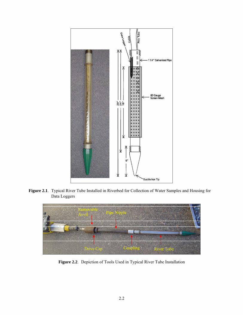
A network of river tubes was installed along the 300 Area shoreline. The river tubes are constructed of 3.2-cm inside diameter (ID) pipe (1.25-in. nominal pipe size). Some of the pipe was galvanized schedule 40, and some was black-iron schedule 80. The two types of pipe were used interchangeably, depending on the strength requirements at individual installation locations. The screened portion of the river tubes consists of a length of pipe perforated with 1.3-cm diameter holes over a 46-cm length, and a hardened steel tip. The perforated section was covered by an 80-mesh screen sandwiched between the pipe and an outer layer for protection (Figure 2.1).

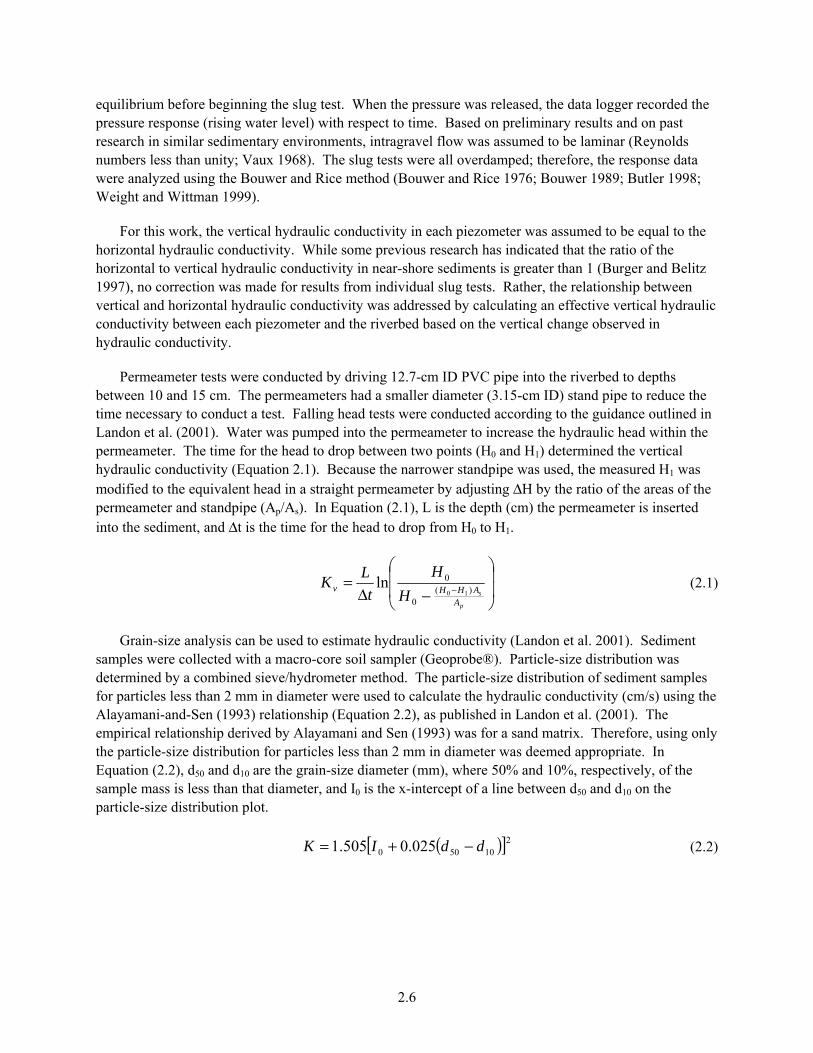
Installation was accomplished by driving the river tubes into the ground with a two-cycle jackhammer (BH-23, Wacker Corp., Wisconsin). The jackhammer mass is approximately 20 kg and can be operated by two people. Hardened-steel drive caps (Grainger) were threaded onto the top of the screened portion of the river tube to provide a point of impact for the jackhammer. The section was driven nearly flush with the riverbed. The cap was removed, a drive coupling (Grainger) and pipe extension were added, the drive cap was attached to the top of the pipe extension, and driving with the jackhammer continued (Figure 2.2).

The above process was repeated until either the target depth was reached or the geology would not allow further penetration. Once driving was completed, the river tube was developed by either pumping silt out the bottom or pumping clean water down the river tube to push silt out the top. Once developed, river tubes were capped and plumbed with sampling tubing. The inlet of the sample tubing was located nominally in the middle of the screened section (Figure 2.1). The sampling tubes were then extended up the shore above the high-water mark to allow year-round sampling. Both polyethylene and polyvinyl chloride (PVC) tubing were used for sampling tubing. The disadvantages of river tubes were a long-screen length and relatively expensive materials (approximately $100 per river tube, as compared to approximately $30 for an aquifer tube). However, river tubes allowed for the installation of continuous water-quality monitoring equipment, which was not possible with aquifer tubes (see Section 2.5).

2.2

Figure 2.1. Typical River Tube Installed in Riverbed for Collection of Water Samples and Housing for Data Loggers

River Tube Coupling

Pipe Nipple

Drive Cap

Removable Anvil

Figure 2.2. Depiction of Tools Used in Typical River Tube Installation

2.3

2.2 Aquifer Tube Installation

Installation of aquifer tubes was done using a technique adapted from the installation of river tubes and previous methods used to install aquifer tubes (Peterson et al. 1998). Aquifer tubes consist of a perforated screen attached to a well-point on one end and a tube on the other. For this work, 0.64-cm outside diameter (OD) polyethylene tubing was used for the sampling tubing. The screens used by the GPAP and the RACS Projects were 15-cm long and 1.3-cm diameter, 80-mesh stainless-steel attached to a stainless-steel point (Geoprobe® Systems, Salina, Kansas) (Figure 2.3). The aquifer tubes installed by the SESP had 7.6-cm plastic screens attached to brass points and connected with polyethylene tubing.

Figure 2.3. Typical Aquifer Tube and Tools Used in Installation of Aquifer Tubes

The aquifer tubes were installed by driving a hollow, 2.54-cm OD, hardened-steel drive rod into the ground, with the stainless-steel tip attached to the end of the screen and tubing inside the drive rod. A slotted drive cap, which allowed the tubing to come out the top of the rod, was used so that the tubing was not pinched or damaged during the hammering process. Drive-rod sections were added as needed to reach the desired depth. Driving was accomplished with a two-cycle jackhammer (or manually with a post driver) in a similar manner to the river-tube installation. Once the desired depth was reached, the drive rod was extracted, leaving the point, screen, and tubing behind. The drive rod was extracted either with pipe wrenches (for shallow points), with sledgehammers (medium-depth points) pounded against a custom fabricated extraction plate (Figure 2.4), or using pneumatic jacks to push against the extraction plate (deep installations). As the drive rod was extracted, the tip, screen, and tubing were left behind in the ground. The tubing was extended up the shoreline to allow access for year-round sampling. A peristaltic pump was attached to the tubing immediately after installation and used to develop the aquifer tube. Water was pumped until the water was clear, or the opacity had decreased substantially and was not decreasing further, at which point the aquifer tube was considered developed. An alternative method of aquifer-tube installation was employed at some locations. With this method, only the tip was inserted into the end of the drive rod, and driving proceeded as described above. Once the desired depth was reached, the screen and tube were inserted into the top of the drive rod, fed down, and threaded onto the tip. The drive rod was then removed, leaving the aquifer tube in place for sampling. This method did not work well at depths exceeding 1.8 m, or in very loose, gravelly substrate. The methods of aquifer-tube installation described here are based on the implant method developed by Geoprobe® Systems (Appendix A).

Geoprobe rod

Slotted Drive Cap Removable Anvil

2.4

5 inches

Figure 2.4. Extraction Plate Used to Remove Geoprobe® Rod from the Ground During Aquifer Tube Installation

2.3 Field Water Quality Measurements

Field measurements of water quality parameters were made following collection of water samples. Temperature, specific conductance, pH, total dissolved solids, and oxidation-reduction potential (ORP) were measured using a calibrated hand-held meter (Ultrameter™, Myron L Company, Carlsbad, California). Water-quality parameters were measured by rinsing out the meter’s cells three times. Each cell was then filled, and the values were recorded on appropriate paperwork. Occasionally, dissolved oxygen was also measured in the field samples using a hand-held luminescent meter (HQ10 Hach Portable LDO Meters™, Hach Company, Loveland, Colorado). For the dissolved oxygen measurements, a small container was filled with a sample, and the end of the meter was immersed into the sample liquid. When filling the container, the tubing was kept below the water level in the container to minimize re-oxygenation of the sample. Water quality parameters were recorded after the sample container had been filled, although initial and final specific conductance were generally also recorded to allow an evaluation of change in water-quality parameters that occurred while the bottles were filled.

2.4 Water Sampling

Water samples were collected from both river tubes and aquifer tubes. Water sampling procedures established for the SESP (Hanf et al. 2007) were adopted for use on this project. Water samples were collected using peristaltic pumps. Prior to collecting a sample, field water quality results were used to determine when each sampling point had been adequately purged. Water was pumped from the sampling tubes until the specific conductance and temperature of the sample reached constant values. Specific conductance was also measured at the end of sample collection to determine if any change had occurred during sample collection.

2.5

2.5 Continuous Water Quality Monitoring

Continuous water quality monitoring sensors were installed within some of the river tubes in the 300 Area near-shore monitoring network (Figure 2.5). These sensors measured temperature, pressure, and specific conductance at a set frequency. The sensors were Solinst® LTC leveloggers (Solinst Canada, Ltd., Ontario, Canada). The leveloggers have self-contained memory, allowing the measurement and storage of data at a user-selectable frequency. Initially, the leveloggers were set to record data every 10 minutes. After several months, unnecessarily high frequencies became apparent because the water parameters were changing slowly. A 30-minute frequency was adopted to reduce the time between downloading events and still meet data requirements. The leveloggers were installed inside the river tubes at various locations and depths in the 300 Area near-shore environment. Leveloggers were also installed on the riverbed and on shore to record river depth and temperature, in addition to barometric pressure. Since the leveloggers measure absolute pressure, measuring barometric pressure to subtract atmospheric effects from the recorded data was necessary.

Figure 2.5. Continuous Data Loggers from Solinst Canada, Ltd.

2.6 Hydraulic Conductivity Testing

Hydraulic conductivity was measured by conducting slug tests, evaluating sediment grain size, and conducting permeameter tests. Slug tests were done in triplicate at each of the river tubes (Butler 1998), grain-size samples were collected at various depths, and permeameters were installed adjacent to a surface-flux chamber.

Slug testing of river tubes has been used to determine hydraulic conductivity within the hyporheic zone along the Hanford Reach (Arntzen et al. 2006; Geist 2000). Slug tests were conducted by attaching an airtight pressure-regulating wellhead assembly to the top of each river tube. The assembly consisted of a 5-cm diameter ball-valve coupled to a 20-cm-long section of schedule-40 PVC containing a small valve-stem for pressurizing. A pressure transducer (Instrumentation NW Model 9800) was lowered into the river tube to measure changes in hydraulic head during the test. A modified rubber stopper was used to seal the transducer cable’s entry into the well assembly. The system was pressurized with a portable battery-powered air compressor (Black and Decker VersaPak cordless inflator), causing the water level in the river tube to be depressed downward. The change in water level was measured and recorded by the transducer at a 10-Hz frequency. When the water level in the well was sufficiently depressed, the air compressor was shut off and the ball-valve was opened, marking the beginning of the slug test. A several second delay between shutting off the compressor and opening the valve ensured that the head reached

2.6

equilibrium before beginning the slug test. When the pressure was released, the data logger recorded the pressure response (rising water level) with respect to time. Based on preliminary results and on past research in similar sedimentary environments, intragravel flow was assumed to be laminar (Reynolds numbers less than unity; Vaux 1968). The slug tests were all overdamped; therefore, the response data were analyzed using the Bouwer and Rice method (Bouwer and Rice 1976; Bouwer 1989; Butler 1998; Weight and Wittman 1999).

For this work, the vertical hydraulic conductivity in each piezometer was assumed to be equal to the horizontal hydraulic conductivity. While some previous research has indicated that the ratio of the horizontal to vertical hydraulic conductivity in near-shore sediments is greater than 1 (Burger and Belitz 1997), no correction was made for results from individual slug tests. Rather, the relationship between vertical and horizontal hydraulic conductivity was addressed by calculating an effective vertical hydraulic conductivity between each piezometer and the riverbed based on the vertical change observed in hydraulic conductivity.

Permeameter tests were conducted by driving 12.7-cm ID PVC pipe into the riverbed to depths between 10 and 15 cm. The permeameters had a smaller diameter (3.15-cm ID) stand pipe to reduce the time necessary to conduct a test. Falling head tests were conducted according to the guidance outlined in Landon et al. (2001). Water was pumped into the permeameter to increase the hydraulic head within the permeameter. The time for the head to drop between two points (H0 and H1) determined the vertical hydraulic conductivity (Equation 2.1). Because the narrower standpipe was used, the measured H1 was modified to the equivalent head in a straight permeameter by adjusting ΔH by the ratio of the areas of the permeameter and standpipe (Ap/As). In Equation (2.1), L is the depth (cm) the permeameter is inserted into the sediment, and Δt is the time for the head to drop from H0 to H1.

⎟⎟

⎠

⎞

⎜⎜

⎝

⎛

−Δ= −

p

sA

AHHv HH

tLK )(

0

010

ln (2.1)

Grain-size analysis can be used to estimate hydraulic conductivity (Landon et al. 2001). Sediment samples were collected with a macro-core soil sampler (Geoprobe®). Particle-size distribution was determined by a combined sieve/hydrometer method. The particle-size distribution of sediment samples for particles less than 2 mm in diameter were used to calculate the hydraulic conductivity (cm/s) using the Alayamani-and-Sen (1993) relationship (Equation 2.2), as published in Landon et al. (2001). The empirical relationship derived by Alayamani and Sen (1993) was for a sand matrix. Therefore, using only the particle-size distribution for particles less than 2 mm in diameter was deemed appropriate. In Equation (2.2), d50 and d10 are the grain-size diameter (mm), where 50% and 10%, respectively, of the sample mass is less than that diameter, and I0 is the x-intercept of a line between d50 and d10 on the particle-size distribution plot.

( )[ ]210500 025.0505.1 ddIK −+= (2.2)

2.7

2.7 Near-Shore Groundwater Well Water-Level Measurement

To characterize the influence of changing Columbia River water levels on groundwater monitoring wells, water-level monitors were installed in a number of wells in the 300 Area along the shoreline. The monitoring stations consisted of pressure sensors (PDCR, GE Druck, New Fairfield, Connecticut) connected to a data logger (CR10X, Campbell Scientific). Pressure was measured every 60 seconds, averaged, and stored as an average pressure every 15 minutes. Pressure sensors measured gage pressure. In this fashion, changes in barometric pressure had no effect on the results. Pressure measurements were converted to water-level elevation by determining the elevation at the top of the well casing and the depth of installation of the pressure sensors. Accuracy of the measurements was ±1 cm of water. Monitors were installed at nine groundwater wells beginning in August 2004.

2.8 Ground Penetrating Radar

In an effort to collect geologic information along the shoreline, ground penetrating radar (GPR) was used to identify the contact between the permeable Hanford formation and the less-permeable Ringold Formation. GPR uses electromagnetic energy of varying frequencies to characterize buried materials through reflected energy imaging (Davis and Annan 1989). The reflections result from changes in electrical and magnetic properties in subsurface materials, specifically relative dielectric permittivity, electrical conductivity, and magnetic permeability (Conyers and Lucius 1996; Conyers and Goodman 1997; Lucius et al. 1998; Powers 1995). The greater the change, the more energy reflected in return (Sellman et al. 1983). The time elapsed between the receptions of different reflections by the receiver provided relative-depth information. This relative depth was converted to true depth by determining the pulse energy velocity through the subsurface (Conyers and Lucius 1996). The data were collected with a Pulse Echo 1000 unit (Sensors & Software, Inc., Mississauga, Ontario, Canada). A shielded 225-MHz bistatic antenna was used. Data were collected along transect “runways” that were prepared to facilitate better energy coupling between the antenna and the earth materials. The runways were cleared of larger riverbed cobble, exposing the moist bed sediment and creating a smooth, level surface for the antenna. Data were collected along survey transects every 10 cm using the monostatic stepped point collection technique. This allowed the data to be stacked at each location to increase the signal-to-noise ratio. At each of the two survey locations, a bistatic common mid-point survey was also done to obtain velocity values for true-depth determination in post processing. These common mid-point surveys were done in 10-cm increases along the survey transect.

2.9 Drive-Point Penetration Testing

During the installation of water sampling tubes into the hyporheic zone, refusal of the installation drive rod occurred at consistent depths at the same location, but the depth varied at different locations. To map this contact, aquifer tube drive rods were used to probe various shoreline locations. The location was surveyed prior to driving. The rod was driven until there was a distinct change in the speed at which the rod was advancing. Generally, this meant complete refusal. However, at some locations, driving went from fast to slow very rapidly. The depth of penetration was marked on the drive rod, and then the rod was extracted from the riverbed using the same extraction techniques described in Section 2.2. The total depth of penetration was recorded, and when combined with the survey data, provided an elevation of the contact. This elevation was assumed to be accurate to 25 cm. While this represented the refusal of driving, it may or may not represent the contact between principal stratigraphic units.

2.8

2.10 Clam Uptake Studies

Some of the initial work evaluating the hyporheic zone between groundwater and Columbia River water identified river clams (Corbicula fluminea) as a potential biological indicator species (Patton et al. 2003). Correlations were observed at low river stage between measured uranium concentrations in riverbank springs water and river water and uranium concentrations in clam soft tissues. However, information on the uptake rate of uranium by clams was not obtained. A uranium uptake study was conducted to evaluate clams as a potential indicator species for areas of elevated contamination in the hyporheic zone. Clams were collected from a reference location with low uranium concentrations in the river and groundwater. The clams were split into three groups and exposed to water with varying uranium concentrations (approximately 4, 14, and 100 μg/L uranium, respectively). Concentrations of uranium in the clam soft tissue were measured after 48, 96, 120, and 144 hours of exposure and a subsequent 120-hour depuration period in water with low uranium levels.

2.11 Analytical Methods

Water samples were sent to several analytical laboratories for analysis. Radiological analyses were conducted at Severn Trent Laboratories, Inc. (Richland, Washington), following the requirements of the SESP analytical contract. Metals analyses were conducted by PNNL’s Marine Sciences Laboratory (MSL) using inductively coupled plasma-mass spectrometry (ICP-MS). Water samples were analyzed by ICP-MS using methods adapted from EPA Method 1640 (EPA 1997b). Anions were measured at PNNL using ion chromatography (EPA Method 300.1 [EPA 1997a]). Alkalinity was measured by Energy Northwest (Richland, Washington) using EPA Method 310 (EPA 1983). An analysis for uranium was conducted by RJ Lee Co. using ICP-MS. Both MSL and RJ Lee Co. analyzed uranium as total metal mass per volume of water (mg/L). Severn Trent Laboratories results provided isotopic concentrations (pCi/L) for uranium-234, uranium-235, and uranium-238. Based on the isotopic concentrations and the specific activities of the three uranium isotopes, the mass measurements obtained with ICP-MS were assumed to consist of more than 99% uranium-238. For some data analyses, mass measurements were converted to activity concentrations by multiplying by the specific activity of uranium-238 (3.4 x 10-7 Ci/g). The MSL-developed method for analyzing clam tissues (adapted from EPA Methods 1638 and 200.8 [EPA 1996b and 1994]) was used for analysis of uranium concentrations in clam soft tissue. Results of analyses, along with supporting metadata, are stored in the Hanford Environmental Information System, where the information is available for access and use.

2.12 Hydraulic Gradient

Hydraulic gradient is the difference in pressure over a unit distance between two points along a stream line in a saturated matrix. This defines the potential energy available to move water from one location to another. For this work, the vertical hydraulic gradient (dh/dl) was most relevant, as it described the difference in pressure at various depths within the hyporheic zone. Near continuous measurements of vertical hydraulic gradient were made using the LTC leveloggers (described in Section 2.5). The vertical hydraulic gradient was calculated as the difference in pressure between the measurement point (within the screened section of a river tube) and the bottom of the riverbed (ΔP), minus the difference in height between the two measurements (Δz), and divided by the distance between the riverbed and the screen midpoint (Δl).

2.9

l

zPdldh

ΔΔ−Δ= (2.3)

2.13 Other Miscellaneous Procedures

Columbia River stages are continuously monitored in the 300 Area at the stage monitor operated by Fluor Hanford, Inc. River stage is recorded hourly as an elevation in meters using the NAVD88 vertical datum. The river stage in the 300 Area is influenced by both discharge from the Priest Rapids Dam and the pool elevation behind McNary Dam. Data for both Priest Rapids discharge and McNary pool elevation are available online in real-time from the U.S. Army Corps of Engineers (USACE) (USACE 2005). Historical data are available online from the U.S. Geological Survey for Priest Rapids discharge (USGS 2007).

3.1

3.0 Geology

3.1 Geologic Setting of the 300 Area

The hydrogeologic framework of the 300 Area near the Columbia River corridor sets the template for local groundwater movement and contaminant transport. Identifying the shape and extent of the geologic formations in the vicinity of the river are necessary to estimate the vertical extent of contamination, to identify areas potentially impacted by contaminated groundwater discharge in the river, and for modeling exchange between groundwater and river water.

Sediments overlying basalt bedrock in the 300 Area consist primarily of the Ringold Formation, the Hanford formation, and a thin veneer of wind-blown and Columbia River deposits1 (Figure 3.1). Because these units differ physically in the associated lithologic and stratigraphic properties, the units are also very different in terms of respective hydraulic properties. The brief discussion that follows highlights the similarities and differences in the geologic and hydrogeologic properties of these geologic layers, ordered from oldest to youngest. The information presented is a summary from previous reports (e.g., Lindberg and Bond 1979; Schalla et al. 1988; Gaylord and Poeter 1991; Swanson et al. 1992; Thorne et al. 1993; Lindsey 1995) and recent reports (Williams et al. 2007).

3.1.1 Ringold Formation

The Ringold Formation consists of interbedded clays, silts, sands, and gravels deposited by the ancestral Columbia, Clearwater/Salmon, and Yakima Rivers from approximately 8.5 to 3.0 million years ago, as these rivers freely meandered across the central Columbia Basin (Lindsey 1995). The Ringold Formation is typically broken up into three informal members based on differences and similarities in grain size, bedding, composition, and sedimentation (Lindsey 1995). These include the Wooded Island, Taylor Flat, and Savage Island members, in order of oldest to youngest. Only the Wooded Island member (lower Ringold) is preserved in the 300 Area due to significant post-Ringold erosion (Swanson et al. 1992) (Figure 3.1). The Wooded Island member has been subdivided into five separate stratigraphic units, designated as units A (the Lower Mud), B, C, D, and E (Lindsey 1995). However, well-log data indicate that units C and D are not present in the 300 Area (Gaylord and Poeter 1991; Swanson et al. 1992; Williams et al. 2007).

At the 300 Area, the Ringold Unit E forms the upper Ringold contact with the Hanford formation (Williams et al. 2007) as well as much of the riverbed substrate of the Columbia River in the 300 Area. The lithology of the Ringold Unit E is highly heterogeneous within the 300 Area due to its fluvial origin. In general, this is composed of granule to cobble size gravels that are interbedded by and interfingered with thinner layers of sand and silt. The Ringold lower mud unit, stratigraphically below Unit E, forms the confining base of the upper-most aquifer, and has hydraulic conductivities much lower than the sands and gravels of Unit E.

1 The Cold Creek Unit (DOE 2002) normally lies stratigraphically between the Ringold and Hanford formations, but due to a large degree of post-Ringold erosion (Swanson 1992), this unit is not preserved in this part of the 300 Area, and will not be discussed further.

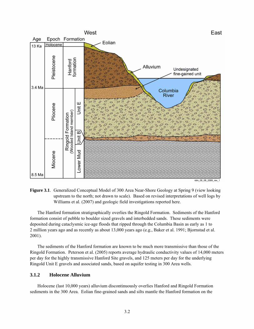
3.2

Figure 3.1. Generalized Conceptual Model of 300 Area Near-Shore Geology at Spring 9 (view looking upstream to the north; not drawn to scale). Based on revised interpretations of well logs by Williams et al. (2007) and geologic field investigations reported here.

The Hanford formation stratigraphically overlies the Ringold Formation. Sediments of the Hanford formation consist of pebble to boulder sized gravels and interbedded sands. These sediments were deposited during cataclysmic ice-age floods that ripped through the Columbia Basin as early as 1 to 2 million years ago and as recently as about 13,000 years ago (e.g., Baker et al. 1991; Bjornstad et al. 2001).

The sediments of the Hanford formation are known to be much more transmissive than those of the Ringold Formation. Peterson et al. (2005) reports average hydraulic conductivity values of 14,000 meters per day for the highly transmissive Hanford Site gravels, and 125 meters per day for the underlying Ringold Unit E gravels and associated sands, based on aquifer testing in 300 Area wells.

3.1.2 Holocene Alluvium

Holocene (last 10,000 years) alluvium discontinuously overlies Hanford and Ringold Formation sediments in the 300 Area. Eolian fine-grained sands and silts mantle the Hanford formation on the

3.3

abandoned floodplain surfaces tens of meters above the modern-day Columbia River level. Given the associated thin and discontinuous character, these wind-blown deposits are less significant to the overall hydrogeologic framework. However, late Holocene to recent fluvial deposits of the modern-day Columbia River make up the present-day riverbank and bed, and are more relevant to the hydrogeology. Based on underwater video-camera footage and accompanying grain-size analysis (see below), these deposits consist mainly of pebble to cobble sized gravels with occasional boulder-sized clasts scattered proximal to the bank.

The thickness of alluvium overlying Hanford or Ringold Formation sediments is not explicitly known. Results of the hydraulic conductivity testing in the hyporheic zone indicate a two order-of-magnitude change in hydraulic conductivity in the top 1 to 2 m of the riverbed sediment (see Section 3.3). This might be indicative of the thickness of alluvium overlying the Hanford or Ringold Formations in the Columbia River along the 300 Area shoreline. However, several underwater camera transects near the Spring 9 vicinity revealed exposures of resistant knobs in the main river channel formed by well-cemented sands and gravels that appear to be outcrops of the Ringold Formation. Among other things, this indicates that alluvium may be very thin to nonexistent in some locations.

3.2 Observations and Measurements of the Ringold Contact

The interface of the Hanford formation with the less-permeable Ringold Formation (referred to informally as the Ringold contact) is a very important hydrogeologic feature. Unfortunately, it is often difficult to identify the Ringold contact since the top of the Ringold Unit E and the basal Hanford formation are both gravel-dominated fluvial deposits in the 300 Area that have common sedimentary properties (e.g., clast roundness, grain size, sorting). However, others have noted some diagnostic differences between the two units, based on drill cuttings and outcrop analog sites. For example, sand-size particles of the Ringold Formation are richer in quartz and feldspar minerals, and contain lower amounts of basalt fragments (<10%), while Hanford formation sands are composed of at least 25% basalt (Swanson et al. 1992). In hand samples, this finding is reflected by the lighter colored nature of the Ringold sands. Also, Hanford Site sands and gravels contain a significantly higher proportion of granule-size particles (2–4 mm) of basaltic composition compared to Ringold Formation sediments, which display less than 1% granule-sized grains (Swanson et al. 1992). Gaylord and Poeter (1991) report that the Hanford formation is generally coarser grained (larger gravels), less cemented and compacted, and does not have extensive fine-grained lithofacies as compared to the Ringold Formation. Previous and ongoing studies have concentrated on defining the two and three-dimensional surface of the Ringold contact in the 300 Area, including the area in the immediate vicinity of the Columbia River shoreline (e.g., Lindberg and Bond 1979; Schalla et al. 1988; Gaylord and Poeter 1991; Swanson et al. 1992; Thorne et al. 1993; Lindsey 1995; Williams et al. 2007).

3.2.1 Refinement of the Hydrogeologic Conceptual Model

Recently, Williams et al. (2007) have interpreted sediment cores and well logs (geologist observa-tions) from four wells drilled in 2006, and reinterpreted logs and sediment data from pre-existing wells in the area. Although the interpretations are preliminary, several important results with implications for groundwater flow have been identified. There is a massively bedded and fine-grained sand layer sandwiched between the gravelly facies of the Hanford and Ringold Formations (Figure 3.1). This fine-grained sand layer appears to be laterally extensive, rather than a small discontinuous lens, and has

3.4

very low permeability relative to the Hanford formation (Williams et al. 2007). Furthermore, cross-sections and structure contours drawn from geologic contacts for the new and reinterpreted existing wells indicate that the top of the Ringold Formation contains bifurcating channels running northwest-to-southeast and west-to-east. These erosional channels are cut into the Ringold Formation and are filled with Hanford gravels (Lindberg and Bond 1979; Williams et al. 2007).

The presence of this extensive sand layer and the incised channels are important to the fate and transport of groundwater contamination. The hydraulically tight nature of the fine sand layer impedes horizontal groundwater flow, and the sand serves as a confining layer to vertical movement. The channels incised into the Ringold Formation might act as preferential pathways for groundwater flow, as these thoroughfares are filled with the less-compacted gravels and sands of the Hanford formation, which have hydraulic conductivities several orders of magnitude higher than their respective Ringold Formation counterparts (Peterson et al. 2005).

3.2.2 Recent Multidisciplinary Field Investigations Along the Near-Shore Area

Multiple methods of field investigation have been conducted to further evaluate the Ringold Formation contact along the 300 Area shoreline. These approaches include qualitative observations made during river and aquifer tube installation, penetration testing, underwater camera and bathymetric surveys, GPR, hydrologic testing, and groundwater sampling.

3.2.2.1 Drive-Point Penetration Tests

An impenetrable layer was observed during the installation of river and aquifer tubes, which proved sufficiently resistant to stop advancement into the subsurface. This layer is thought to be the contact between loose Hanford Site or alluvial gravels and the more cemented gravels and compact sands of the Ringold Formation. A series of drive-point penetration tests were conducted to “feel” this resistant layer at multiple points distributed along the shoreline of the river (see Section 2.9) (Figure 3.2). The drive-point penetration results correlate with the elevations for the Ringold Formation contact of Williams et al. (2007). Both show a structural low near and immediately downstream of Spring 9 (drive-points 3 through 7) with elevations2 that range from approximately 97 to 99 m (Figure 3.3). Downstream, the contact rises noticeably with elevations that range from approximately 101 to 103 m.

Although the two data sets were similar, there were some apparent differences (Figure 3.3). Drive-points 4 and 5 suggested an elevation for the Ringold contact several meters higher than Williams et al. (2007). Note that the Ringold contact interpretations from Williams et al. (2007) were based on borehole geologic data from wells located tens to hundreds of meters away from the shoreline, and data were extrapolated to project them out to the shoreline. However, the drive-point penetration tests were performed along the shoreline and were more closely spaced (Figure 3.3). The drive-point elevations should be regarded as minimum elevations because boulders or very large gravels may have been responsible for stopping the penetration of the drive-point some unknown distance above the real change in lithology. However, multiple drive-point penetration tests in the same area generally resulted in consistent refusal elevations, giving confidence to the accuracy of the method. Given these factors, the disagreement in detail between the geologic interpretation and the drive-point penetration testing was not

2 Elevations are reported in meters above mean sea level according to the North American Vertical Datum of 1988 (NAVD88).

3.5

unreasonable. The general agreement created confidence in using drive-point penetration data together with traditional geologic investigations for constraining the shape and elevation of the Ringold contact along the shoreline. Future drive-point penetration efforts should concentrate on measuring the resistant layer at points farther down the shoreline, where Williams et al. (2007) interpreted another low in the Ringold contact (erosive channel mentioned above), and more measurements at Spring 9. These data will promote confirmation and extend the conventional geologic interpretations from boreholes into the riverbed.

Figure 3.2. Map Showing Drive-Point Penetration Sample Site Locations and Measured Elevations of an Impenetrable Layer Along the 300 Area Shoreline

3.6

96

97

98

99

100

101

102

103

104

105

106

115800115850115900115950116000116050116100116150116200116250116300116350

Northing (m; Washington State Plane South, NAD83)

Elev

atio

n (m

eter

s; N

AVD

88)

Ringold Contact (Williams et al., 2007)

Drive-Point Penetration

Ground Surface

"Resist" Layer During AT Installs

Aquifer Tubes (Abbreviated Name)

SP9AUS125 AT-3-3 DS75 AT-3-4

Upstream Downstream

Figure 3.3. Relation Between Resistant Layer Observed during Aquifer Tube (AT) Installation and Drive-Point Penetration Tests with Interpreted Ringold Contact (Based on Williams et al. 2007). Data are oriented in the downstream direction from left to right. Note the 25:1 horizontal exaggeration in scale.

3.2.2.2 Surface Geophysical Investigations

Several geophysical techniques were employed to constrain the elevation and shape of the Ringold contact in the hyporheic zone. Borehole geophysical methods (e.g., gamma logging) were initially employed; however, these required a cased borehole. The layer estimated to be the Ringold contact proved impenetrable to a number of direct-push techniques, making geophysical logging below the contact impossible. A GPR survey was attempted as a surface-based technique to identify the Ringold contact (see Section 2.8). GPR survey results at a location upstream of Spring 9 (103meterArrayUS125) identified a reflective layer at an approximate elevation of 103.2 m. The elevation of the reflection was dramatically higher than the Ringold contact suggested by drive-point penetration testing at points 1 and 2 (Figure 3.3) and interpretations by Williams et al. (2007). Furthermore, GPR did not work at the AT3-3A aquifer tube location. Data analyses collected at AT3-3A indicated that the signal was lost before any changes in stratigraphy could be identified. The apparent reason for signal loss was the high-specific conductance water in the hyporheic zone during the low river stage on the day the survey was completed. This may also explain the discrepancy at the US125 location. GPR did not appear to be a feasible technique for evaluating geology in the hyporheic zone at the 300 Area.

3.2.2.3 Riverbed Bathymetry

Riverbed bathymetry for the Columbia River in the 300 Area was analyzed to explore the relation between river channel form and the underlying geology, and to provide detailed riverbed elevations for defining the potential riverbed surface area affected by uranium discharges. The bathymetry data were recently collected for selected portions of the Hanford Reach by the USACE using its Compact Hydrographic Airborne Rapid Total Survey (CHARTS) system, under contract from the U.S. Fish and Wildlife Services (USFWS). The horizontal resolution (grid cell size) of the CHARTS data is 1 m, and has horizontal accuracies to within ±3 m and elevations to within ±15 cm (Anglin et al. 2006).

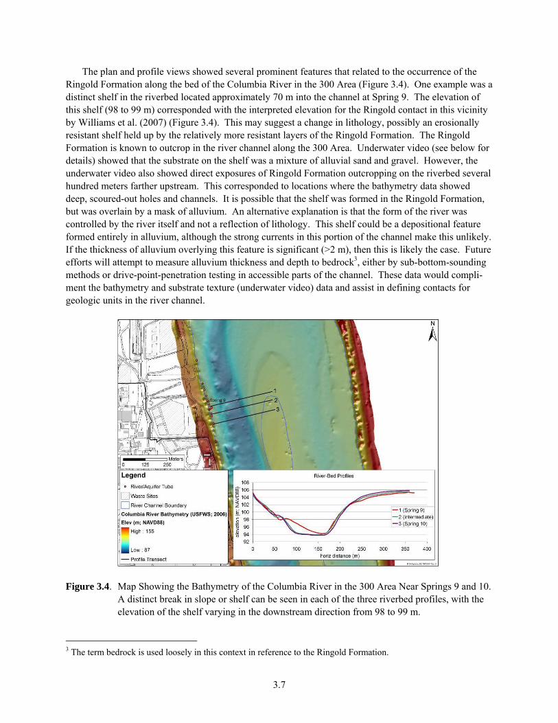
3.7

The plan and profile views showed several prominent features that related to the occurrence of the Ringold Formation along the bed of the Columbia River in the 300 Area (Figure 3.4). One example was a distinct shelf in the riverbed located approximately 70 m into the channel at Spring 9. The elevation of this shelf (98 to 99 m) corresponded with the interpreted elevation for the Ringold contact in this vicinity by Williams et al. (2007) (Figure 3.4). This may suggest a change in lithology, possibly an erosionally resistant shelf held up by the relatively more resistant layers of the Ringold Formation. The Ringold Formation is known to outcrop in the river channel along the 300 Area. Underwater video (see below for details) showed that the substrate on the shelf was a mixture of alluvial sand and gravel. However, the underwater video also showed direct exposures of Ringold Formation outcropping on the riverbed several hundred meters farther upstream. This corresponded to locations where the bathymetry data showed deep, scoured-out holes and channels. It is possible that the shelf was formed in the Ringold Formation, but was overlain by a mask of alluvium. An alternative explanation is that the form of the river was controlled by the river itself and not a reflection of lithology. This shelf could be a depositional feature formed entirely in alluvium, although the strong currents in this portion of the channel make this unlikely. If the thickness of alluvium overlying this feature is significant (>2 m), then this is likely the case. Future efforts will attempt to measure alluvium thickness and depth to bedrock3, either by sub-bottom-sounding methods or drive-point-penetration testing in accessible parts of the channel. These data would compli-ment the bathymetry and substrate texture (underwater video) data and assist in defining contacts for geologic units in the river channel.

Figure 3.4. Map Showing the Bathymetry of the Columbia River in the 300 Area Near Springs 9 and 10. A distinct break in slope or shelf can be seen in each of the three riverbed profiles, with the elevation of the shelf varying in the downstream direction from 98 to 99 m.

3 The term bedrock is used loosely in this context in reference to the Ringold Formation.

3.8

3.2.2.4 Underwater Video

In addition to the bathymetry data, underwater video footage was collected along numerous transects near Springs 7 and 9, with the intent of identifying and mapping various riverbed substrate types. The quality of the video footage was somewhat hampered by the swift current, water turbidity, and insuffi-cient natural lighting; however, several noteworthy findings were identified. First, there did appear to be mappable units of substrate type identifiable in the video images. Generally, the alluvial substrate was composed of a heterogeneous mixture of sand, pebble, gravel, and boulders (near the bank). Clasts appeared to decrease in size and were more mixed in composition (more lighter-colored cobbles and pebbles) as depth increased in the channel away from the bank. This is an interesting observation because fluvial deposits typically coarsen with increasing flow depth and current velocity. This may provide an indication that the Columbia River is cutting into more fine-grained material (Ringold Formation) deeper in the channel.

The underwater video images revealed several exposures of a lighter-colored material that were prominent in relief above the adjacent alluvium (Figure 3.5). The outcrops appeared to be formed by a well-indurated material that offered enough erosional resistance to form meter-scale knobs and reef-like features in a variety of water depths that ranged from 5 to 10 m. The material appeared to be composed of a sandy or silty matrix with pebble and small cobble clasts (more sand than gravel), and had a mottled appearance, very different from the adjacent alluvium. This material was interpreted to be gravelly, sand lithofacies within the Ringold Unit E. Well-cemented, gravelly sand exposed along the shoreline several kilometers upstream looked strikingly similar, and may be an analog to what was seen on the video (Figure 3.6). Both were well-cemented sands and gravels that contained cavities that were reminiscent of pockets or remnant molds left behind as cobble clasts were eroded or weathered away (Figures 3.5 and 3.7).

Samples of the well-cemented sand observed in the underwater video were retrieved from the river bottom at elevations between 98 and 99 m elevation (Figure 3.7, collected at a northing of 116,250 m). Based on visual comparison to adjacent borehole photos, these samples were preliminarily identified as the Ringold Formation. Based on the initial interpretation, the elevation (98 m) from which these samples were collected was in sync with the elevation of the Ringold Formation at this location, projected by both the probing and limited field investigation drilling (Figure 3.3). This was significant, as it provided evidence that the Ringold Formation outcrops in the Columbia River.

3.3 Hydraulic Conductivity

Hydraulic conductivity was measured by conducting slug tests in river tubes installed along the Columbia River shoreline, conducting permeameter tests of the riverbed surface, and by grain-size analysis of sediment samples for the less than 2-mm size fraction (see Section 2.6). Testing was centered on two primary locations Spring 9 and the AT3-3 location, 50 m downstream of Spring 9. The results of the hydraulic conductivity measurements indicated that the hydraulic conductivity of the Hanford formation in the hyporheic zone increased with depth below the riverbed surface (Figure 3.8). Tests were conducted in both 2004 and 2006 to evaluate temporal changes in hydraulic conductivity results. Little change was observed in the results between 2004 and 2006.

3.9

Figure 3.5. Screen-Shots from Underwater Video of Substrate Near Springs 7 and 9. The two bright lines in each image are laser beams from sources mounted 19 cm apart, and offer a sense of horizontal scale. Image (a) is a representative view of the unconsolidated gravelly alluvium that comprises most of the riverbed substrate. Images (b), (c), and (d) show exposures of a lighter-colored material with a sandy or silty texture, thought to be a gravelly sand facies within the Ringold Unit E. Although not obvious in these two-dimensional images where the sense of depth is lost, these outcrops typically form knobs or reef-like structures that stand out in relief above the gravelly alluvium on the bed of the river due to a higher relative resistance to erosion. Note the presence of pebble-sized cavities or pockets inset into the material; possibly clast molds left behind after pebbles were weathered away or hydraulically plucked out by the river.

aa)) bb))

cc)) dd))

3.10

Figure 3.6. Outcrop of Well-Cemented Gravelly Sand Layer (upstream of the 300 Area) Within the Ringold Unit E, Exposed About 0.5 m Above the Average River Stage (pencil for scale). This may be an analog for the lighter-colored resistant layer observable in the underwater video and samples collected from same location (compare to Figures 3.5b - d and 3.6).

Figure 3.7. Samples of Ringold Formation Retrieved from Outcrop on the Bottom of the Columbia River. Scale bars are 1 cm. Note that these photos are of wet samples.

3.11

1.E-04

1.E-03

1.E-02

1.E-01

1.E+00

0 100 200 300 400 500

Depth of screen mid-point below riverbed (cm)

Mea

sure

d Hy

drau

lic

Cond

uctiv

ity (c

m/s

) Spring 9 AT3-3

grain size result

Figure 3.8. Hydraulic Conductivity Measured in River Tubes Along the 300 Area Shoreline.

Results of the slug testing and permeameter testing indicate that the surface of the riverbed is the most restrictive portion of the hyporheic zone. At the surface, the hydraulic conductivity is around 5 x 10-4 cm/s, as measured in both river tubes and permeameters (Figure 3.7). Because the slug testing in river tubes measures the horizontal hydraulic conductivity, and the permeameter testing measures the vertical hydraulic conductivity, the assumption of no anisotropy in the hyporheic zone was valid on a small (cm) scale. However, there was clearly a vertical change in hydraulic conductivity, indicating that hydraulic conductivity measured in a piezometer was not indicative of the total effective K between the measurement point and the riverbed. While no permeameter tests were conducted at the same depth as slug tests, the permeameter data generally fit the trend of the deeper slug test data. The exception to the proportional relationship between depth and hydraulic conductivity occurred at the deepest aquifer tubes at AT3-3. These locations were installed as deep as physically possible. The slightly lower hydraulic conductivities measured at these depths most likely indicate influence from Ringold Formation sediments.

Three sediment samples were collected for grain-size analysis between 50 and 70 cm deep at a location 75 m downstream of AT3-3. The average hydraulic conductivity estimated by the empirical grain-size relationship is similar to hydraulic conductivities measured at similar depths with slug testing (Figure 3.8). Grain-size analysis may prove useful in future work as a method to characterize areas with different vertical hydraulic conductivity at the surface layer, in particular at locations where water depth prevents permeameter testing.

4.1

4.0 Locations

This section outlines the locations, elevations, type, and date of installation of all the monitoring points installed along the 300 Area river shoreline.

4.1 River Tubes and Aquifer Tubes

The network of river tubes and aquifer tubes was modified, and additional locations were added over the course of the investigation. As data became available, additional monitoring locations were added to better characterize the hyporheic zone. The initial aquifer tubes along the 300 Area shoreline were installed by the SESP in 2001. The remainder of the river tubes and aquifer tubes were installed by the S&T Remediation Task beginning in the fall of 2003. Table 4.1 provides the names, installation dates, general location, and tube type. With the exception of the SESP aquifer tubes at Spring 7, most of the sampling tubes are located near Spring 9 (Figures 4.1 and 4.2).

Table 4.1. Sampling Location Names, Installation Dates, and Elevations of River and Aquifer Tubes Installed Along the 300 Area River Shoreline

Names Type Date of Installation Elevation (m) at Top of Screen(a)

300 SPR 9A-19cm River tube 3/30/2004 103.9 300 SPR 9A-86cm River tube 3/30/2004 103.3 300 SPR 9A-142cm River tube 3/23/2004 102.7 300 3-3A-410cm River tube 3/30/2004 100.2 300 3-3A-124cm River tube 6/3/2004 103.0 300 3-3B-376cm River tube 3/30/2004 99.9 300A 3-3A-579cm Aquifer tube 8/8/2004 98.5 300A 3-3B-518cm Aquifer tube 8/8/2004 98.5 300A 3-3C-589cm Aquifer tube 8/8/2004 97.4 300A 3-3C-409cm Aquifer tube 8/8/2004 99.2 103mArray-AT3A Aquifer tube 7/25/2005 102.2 103mArray-US25 Aquifer tube 7/25/2005 102.2 103mArray-US50 Aquifer tube 7/25/2005 102.2 103mArray-US75 Aquifer tube 8/25/2005 102.2 103mArray-US100 Aquifer tube 8/25/2005 102.2 103mArray-US125 Aquifer tube 8/25/2005 103.2 103mArray-DS25 Aquifer tube 7/25/2005 102.2 103mArray-DS50 Aquifer tube 7/25/2005 102.2 103mArray-DS75 Aquifer tube 7/25/2005 102.2 AT-3-3-S(b) Aquifer tube 1/1/2004 103.0 AT-3-3-M(b) Aquifer tube 1/2/2004 100.5 AT-3-3-D(b) Aquifer tube 1/3/2004 96.2 (a) Elevation in NAVD88 datum. (b) Installed by Groundwater Performance Assessment Project.

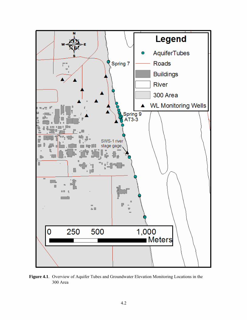
4.2

Figure 4.1. Overview of Aquifer Tubes and Groundwater Elevation Monitoring Locations in the 300 Area

4.3

Figure 4.2. Sampling Locations installed by RCAS Near Spring 9, Along the 300 Area Shoreline

4.4

4.2 Groundwater Well Level Monitoring Locations

Selected shoreline wells in the uranium plume in the 300 Area were chosen to monitor water level, temperature, and specific conductance. These locations were chosen to evaluate the effect of changing Columbia River water stages at the groundwater level within the wells. The monitored locations are illustrated in Figure 4.1. 4.3 Groundwater Monitoring Aquifer Tubes

Locations of the aquifer tubes installed for the GPAP were selected to span nearly the entire uranium contamination plume at the 300-FF-5 Operable Unit shoreline interface (Figure 4.3). Spacing between groundwater aquifer tube locations varied between 250 and 350 m. Tubes were installed at three depths using direct-push methods. These depths were deep (as deep as possible), medium (somewhere between deep and shallow), and shallow (Peterson et al. 2005). Each aquifer-tube location is identified by the alphanumeric labels AT-3- 1, AT-3-2, etc., with location one (1) being the farthest upstream. Each aquifer tube at a location is also given a depth identifier, such that AT-3-1 D is the deepest aquifer tube at the upstream most location.

4.5

Figure 4.3. Locations of Aquifer Tubes Installed by GPAP Along the 300 Area Shoreline, Estimated Groundwater Concentrations of Uranium in the 300 Area, and Uranium Concentrations from GPAP Wells and Aquifer Tubes Sampled in June 2004

5.1

5.0 Continuous Water Quality Monitoring

The continuous data logging capabilities of the leveloggers provide more data than can be presented within this report. However, the data are available for use to answer specific scientific questions, and will be used in subsequent reports and journal articles. This section provides a summary of the data collected in the 300 Area hyporheic zone, along with some of the data applications.

5.1 Initial Deployment

To characterize the dynamic nature of the hyporheic zone, leveloggers with temperature, pressure, and specific conductance sensors were installed in river tubes within the hyporheic zone of the 300 Area. Initially, only four leveloggers were deployed to evaluate the ability of these instruments to monitor the movement and mixing of groundwater and river water in the hyporheic zone. This was conducted during the winter of 2003–2004, at low-river stage, when the near-shore riverbed was easily accessible. Four river tubes were installed near Spring 9 with the top of the screens located above the riverbed, and at 28.5, 65.5, and 130 cm below the riverbed. The leveloggers recorded data at 15-minute intervals over a 2-week period, from November 10- 23, 2003.

Results from this initial deployment illustrated that temperature and specific conductance varied inversely with river stage. As the river stage increased, temperature and specific conductance decreased, demonstrating river water intrusion into the hyporheic zone. These observations were explained by the fact that river water has a lower temperature (in the winter) and lower specific conductance than groundwater. When the river stage decreased, both temperature and specific conductance increased, demonstrating that the ratio of groundwater to river water increased in the hyporheic zone. Based on this initial assessment, a more robust network was installed, with deeper installations and a broader spatial coverage.

5.2 Sensor Network Development

After the initial assessment that the leveloggers demonstrated the ability to monitor temperature, pressure, and specific conductance, a larger network of levelogger sensors was installed in river tubes. In April 2004, leveloggers were installed in five river tubes (SP9A.19, SP9A.86, SP9A.142, AT3 3A.410, and AT3 3B.376). In June 2004, sensors were added at AT3-3A.124 and at the riverbed level. River elevation was calculated by measuring the pressure at a predetermined elevation along the riverbed and subtracting the atmospheric component of the pressure. These data can be used for a variety of purposes. This section presents some of these data and the basic relationships that illustrate the association between changing river stage and groundwater/surface water interaction.

The leveloggers provide a means of estimating groundwater-to-river water dilutions based on specific conductance relationship. Results of the specific conductance and temperature monitoring from August 2004 through August 2005 at the AT3-3A.124 river tube illustrate the relationship between river stage and the dilution of groundwater by river water (Figure 5.1). At high river stage, the specific conductance decreases because of the intrusion of low-specific conductance river water into the subsurface. A regression of daily average river stage and daily average specific conductance at AT3-3A.124 shows this relationship in general terms (Figure 5.2). More detailed examination of the sub-hourly data provides a

5.2

more comprehensive analysis of this relationship (Section 8.2, Fritz and Arntzen 2007). In some instances, a low river stage resulted in low-specific conductance measurements. These days occurred during brief periods of low water, where higher-specific conductance groundwater did not have sufficient time to reach the near-shore riverbed before the river stage increased (e.g., low water periods in July; see Figure 5.1).

050

100150200250300350400450500

8/1/04

8/31/04

10/1/04

10/31/04

12/1/041/1/05

1/31/053/3/05

4/2/055/3/05

6/3/057/3/05

8/3/059/2/05

Spec

ific

Con

duct

ance

(μS/

cm)

104.00

104.50

105.00

105.50

106.00

106.50

Riv

er E

leva

tion

(m)

Specific Conductance River Elevation

Figure 5.1. Specific Conductance and River Elevation at AT3-3A.124 from August 2004 to August 2005. These results are typical of measurements in other river tubes.

0

100

200

300

400

500

600

104 104.5 105 105.5 106 106.5

River elevation (m)

Spec

ific

Con

duct

ance

at

AT3

-3A

.124

(μS/

cm)

Figure 5.2. Regression Between Daily Average River Elevation and Daily Average Specific Conductance Measured at AT3-3A.124

In the winter months, the temperature in the AT3-3A.124 river tube was generally warmer than the river water, but remained somewhat variable. These fluctuations correspond with changing river stage (Figure 5.3). As the river elevation decreases, groundwater moves towards the river. Groundwater is warmer than river water during the winter months, so the temperature in the river tube increases with a

5.3

decrease in river elevation. Similarly, as the river elevation increases, river water moves into the hyporheic zone, and the temperature in the river tube decreases.

0

5

10

15

20

12/1/2004 1/1/2005 2/1/2005 3/1/2005 4/1/2005 5/1/2005

Tem

pera

ture

(C)

104.5

105.0

105.5

106.0

Riv

er E

leva

tion

(m)

River Temp Tube Temp River Elevation

Figure 5.3. Changes in Temperature at AT3-3A.124 Caused by Changes in River Elevation During the Winter Months of 2004–2005. Note that groundwater temperature is generally approximately 15° C.

The levelogger data were also used to determine the vertical hydraulic gradient by evaluating the pressure data. Evaluation of the changes in temperature and specific conductance provided an indication of the direction of water movement. However, using Darcy’s Law provides an estimate of the speed of the groundwater movement, and is an important step in estimating the total contamination that discharges to the river. This application is discussed further in Section 9.3.

Continuous monitoring of temperature, specific conductance, and pressure in the hyporheic zone provided a high-temporal resolution data set that allowed for a more thorough understanding of the interaction of groundwater and river water. These data can be used to estimate flux through the hyporheic zone, and to develop a better conceptual understanding of the rate that conditions change in the 300 Area hyporheic zone.

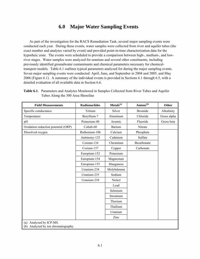
6.1

6.0 Major Water Sampling Events

As part of the investigation for the RACS Remediation Task, several major sampling events were conducted each year. During these events, water samples were collected from river and aquifer tubes (the exact number and analytes varied by event) and provided point-in-time characterization data for the hyporheic zone. The events were scheduled to provide a comparison between high-, medium-, and low-river stages. Water samples were analyzed for uranium and several other constituents, including previously identified groundwater contaminants and chemical parameters necessary for chemical-transport models. Table 6.1 outlines typical parameters analyzed for during the major sampling events. Seven major sampling events were conducted: April, June, and September in 2004 and 2005, and May 2006 (Figure 6.1). A summary of the individual events is provided in Sections 6.1 through 6.5, with a detailed evaluation of all available data in Section 6.6.

Table 6.1. Parameters and Analytes Monitored in Samples Collected from River Tubes and Aquifer Tubes Along the 300 Area Shoreline

Field Measurements Radionuclides Metals(a) Anions(b) Other

Specific conductance Tritium Silver Bromide Alkalinity Temperature Beryllium-7 Aluminum Chloride Gross alpha pH Potassium-40 Arsenic Fluoride Gross beta Oxidation reduction potential (ORP) Cobalt-60 Barium Nitrate Dissolved oxygen Ruthenium-106 Calcium Phosphate

Antimony-125 Cadmium Sulfate Cesium-134 Chromium Bicarbonate Cesium-137 Copper Carbonate

Europium-152 Potassium Europium-154 Magnesium Europium-155 Manganese Uranium-234 Molybdenum Uranium-235 Sodium Uranium-238 Nickel

Lead Selenium Strontium Thorium Thallium Uranium

Zinc

(a) Analyzed by ICP-MS. (b) Analyzed by ion chromatography.

6.2

104.0

104.5

105.0

105.5

106.0

106.5

107.0

107.5

Jan-04 Apr-04 Jul-04 Oct-04 Jan-05 Apr-05 Jul-05 Oct-05 Jan-06 Apr-06

Riv

er E

leva

tion

(m)

River elevation Sample Date

Figure 6.1. Major Sampling Events and River Elevation at the 300 Area

6.1 April 2004 Results

The April 2004 sampling event occurred during a low river stage, when the river stage had been low for several consecutive days. The concentrations of most constituents were much lower in river water (measured in a sample from near the 100-N Area) than in 300 Area near-shore riverbed samples. However, during this period, the concentration of contaminants in the hyporheic zone was not greatly influenced by mixing with river water, demonstrated by the similar concentrations of key constituents at all depths below the riverbed (Table 6.2). This was attributed to the fact that during this low river stage, the groundwater was discharging strongly, providing no opportunity for dilution by river water. The lateral and vertical distributions of field-measured parameters, anions, and metals indicated that the near-shore riverbed flow regime, at this time, appeared to be dominated by groundwater with relatively little river influence. The lack of a vertical gradient in concentrations of contaminants and other indicating parameters supported the hypothesis that groundwater was discharging through the hyporheic zone at a rate sufficient to prevent any measurable dilution by river water.

The analytical data from April 2004 also support the hypothesis that the confining surface dips in elevation at AT-3-3. Concentrations of uranium in aquifer and river tubes near AT-3-3 were similar to each other and to the highest uranium concentrations at Spring 9. There is also evidence that a confining layer exists, separating shallow groundwater from deeper groundwater at AT-3-3. The deep aquifer tube (AT-3-3-D) did not yield much water, indicating its screened end is in a less-permeable layer than the shallower aquifer tubes. The analytical results indicated that two different hydraulic units within the unconfined aquifer were being sampled. While the specific conductance at AT-3-3-D was similar to groundwater, the gross alpha, tritium, and uranium concentrations in water samples from this tube were all less than concentrations from the other sampling locations. Bromide, chloride, nitrate, and sulfate concentrations were also less at the AT-3-3-D sampling location, although the differences were not as extensive as those observed for the radiological constituents (Figure 6.2). The tritium concentration was particularly low at the AT-3-3-D location, and was only 0.8% of the next lowest tritium concentration measured in the hyporheic zone (Table 6.2).

6.3

Table 6.2. Results for Selected Analytes at Locations Sampled in April 2004

Location Name Depth Below

Riverbed (cm)

Specific Conductance

(μS/cm)

Gross Alpha

(pCi/L) Tritium (pCi/L)

Total U (μg/L)(a)

U-234 (pCi/L)(b)

U-235 (pCi/L)(b)

U-238 (pCi/L)(b)

300 SPR 9 -1 (4 in.) 10 373 84 8,880 131 49.6 2.31 43.2

300 SPR 9 -1 (2 ft) 60 401 55.7 9,630 137 48.5 2.60 43.3

300 SPR 9 -1 (4 ft) 122 423 101 10,100 148 53.6 1.75 49.9

300 SPR 9 -1 (6 ft) 183 424 120 10,100 NA 50.1 3.69 45.6

300 SPR 9 -2 (4 in.) 10 385 101 8,960 131 44.5 1.98 39.7

300 SPR 9 -2 (2 ft) 60 416 106 9,720 145 54.3 2.70 47.8

300 SPR 9 -2 (4.5 ft) 137 420 104 9,820 147 49.2 1.15 44.9

300 SPR 9 -3 (2 ft) 60 352 142 8,340 190 61.5 2.65 58.2

300 SPR 9 -3 (5.5 ft) 168 385 75.2 8,510 156 57.4 2.92 54.4

AT-3-3A-410cm 410 429 148 8,840 195 64.8 4.15 59.9

AT-3-3B-376cm 376 403 233 8,340 192 91.2 3.73 84.2

300SPR9A-19cm 19 389 22.4 8,860 107 42.6 1.78 39.5

300SPR9A-86cm 86 420 93 10,000 138 50.7 3.10 46.4

300SPR9A-142cm 142 421 89.9 10,100 135 48.2 2.98 46.9

AT-3-3-S 213 434 122 9,340 195 66.6 2.57 59.5

AT-3-3-M 458 435 113 9,320 183 63.6 2.18 57.5

AT-3-3-D 732 312 5.35 67.4 NA 3.37 0.124 3.24

NA = Not analyzed due to low-water yield at this location. (a) Total uranium determined by ICP-MS. (b) Isotopic uranium concentrations determined by radiochemical analysis.

0.01

0.1

1

10

100

1000

10000

100000

Gross Alpha (pCi/L)

Tritium (pCi/L)

U-234 (pCi/L)

U-235 (pCi/L)

U-238 (pCi/L)

total U (ug/L)

Bromide (ug/L)

Chloride (ug/L)

Nitrate (ug/L)

Sulfate (ug/L)

Con

cent

ratio

n in

Wat

er Above contact AT-3-3-D (below contact)

Figure 6.2. Average Concentration (±2 standard deviation) of Selected Constituents Above and Below the Hydrologic Unit Contact (April 2004)

6.4

6.2 June 2004 Results

A major sampling event was conducted in June 2004 to represent a high-river stage condition. Previous monitoring of pressure, temperature, and specific conductance showed greater river influence on the hyporheic zone at the high-river stage. Thus, the hypothesis was that increased river influence would be reflected in reduced contaminant levels and sharper vertical gradients in contaminant concentrations in the river tube monitoring points. In general, the concentrations measured in June 2004 were lower than the concentrations observed during the April 2004 sampling event.

Similar to the April 2004 sampling event, the deep tube at AT-3-3-D did not yield sufficient water volume for most radionuclide and field parameter measurements, but sufficient sample was available for measuring anions, total uranium, and other metals. The results provided an additional indication that two distinct hydrologic units being sampled at this location were present (Table 6.3). In June 2004, higher nickel, magnesium, arsenic, and potassium concentrations were measured in the AT-3-3-D tube than at other monitoring locations in the hyporheic zone. These metals were not analyzed in water samples collected from AT-3-3-D in April 2004, and may provide some indication of differences between the hydrologic units. The total uranium concentration measured in AT-3-3-D was lower than at locations above the suspected contact sampled in April 2004 (Table 6.3).

6.3 September 2004 Results

The September 2004 sampling event was not as extensive as those of April and June 2004. The goal was to sample during an intermediate river stage to better understand the differences between the first two sampling events. While the September 2004 sampling event occurred during a period of low water, the analytical results were very similar to the June 2004 results (Table 6.4). An observable relationship was evident between increased sample depth and increased contaminant concentrations (Figure 6.3). This most likely indicates that as river stage increases, contaminant concentrations in the hyporheic zone are diluted by river water, and some length of time is required before mixed river/ groundwater in the hyporheic zone is drained from the near-shore portion of the unconfined aquifer.

The relationship between depth and concentration was more apparent during the September 2004 sampling event than that of June 2004 (Figures 6.3 and 6.4). While the June 2004 sampling event occurred during a period of generally high water, the river stage was lower during the sampling event than it had been on previous days (Figure 6.1). Conversely, in September 2004, the general river stage was low, but the sampling event occurred on a day with a high river stage (relative to previous days) (Figure 6.1). This highlights the difficulty in interpreting point-in-time water sampling data in the 300 Area, as the results are influenced by the daily changes in river stages more than the seasonal changes.

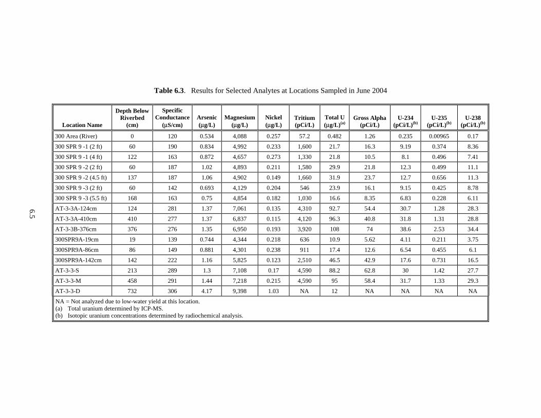
6.5

Table 6.3. Results for Selected Analytes at Locations Sampled in June 2004

Location Name

Depth Below Riverbed

(cm)


(μS/cm) Arsenic (μg/L)

Magnesium (μg/L)

Nickel (μg/L)

Tritium (pCi/L)

Total U (μg/L)(a)

Gross Alpha (pCi/L)

U-234 (pCi/L)(b)

U-235 (pCi/L)(b)

U-238 (pCi/L)(b)

300 Area (River) 0 120 0.534 4,088 0.257 57.2 0.482 1.26 0.235 0.00965 0.17

300 SPR 9 -1 (2 ft) 60 190 0.834 4,992 0.233 1,600 21.7 16.3 9.19 0.374 8.36

300 SPR 9 -1 (4 ft) 122 163 0.872 4,657 0.273 1,330 21.8 10.5 8.1 0.496 7.41

300 SPR 9 -2 (2 ft) 60 187 1.02 4,893 0.211 1,580 29.9 21.8 12.3 0.499 11.1

300 SPR 9 -2 (4.5 ft) 137 187 1.06 4,902 0.149 1,660 31.9 23.7 12.7 0.656 11.3

300 SPR 9 -3 (2 ft) 60 142 0.693 4,129 0.204 546 23.9 16.1 9.15 0.425 8.78

300 SPR 9 -3 (5.5 ft) 168 163 0.75 4,854 0.182 1,030 16.6 8.35 6.83 0.228 6.11

AT-3-3A-124cm 124 281 1.37 7,061 0.135 4,310 92.7 54.4 30.7 1.28 28.3

AT-3-3A-410cm 410 277 1.37 6,837 0.115 4,120 96.3 40.8 31.8 1.31 28.8

AT-3-3B-376cm 376 276 1.35 6,950 0.193 3,920 108 74 38.6 2.53 34.4

300SPR9A-19cm 19 139 0.744 4,344 0.218 636 10.9 5.62 4.11 0.211 3.75

300SPR9A-86cm 86 149 0.881 4,301 0.238 911 17.4 12.6 6.54 0.455 6.1

300SPR9A-142cm 142 222 1.16 5,825 0.123 2,510 46.5 42.9 17.6 0.731 16.5

AT-3-3-S 213 289 1.3 7,108 0.17 4,590 88.2 62.8 30 1.42 27.7

AT-3-3-M 458 291 1.44 7,218 0.215 4,590 95 58.4 31.7 1.33 29.3

AT-3-3-D 732 306 4.17 9,398 1.03 NA 12 NA NA NA NA

NA = Not analyzed due to low-water yield at this location. (a) Total uranium determined by ICP-MS. (b) Isotopic uranium concentrations determined by radiochemical analysis.

6.6

Table 6.4. Results for Selected Analytes at Locations Sampled in September 2004

Location Name


(cm)


(μS/cm) Arsenic (μg/L)

Nickel (μg/L)

Lead (μg/L)

Tritium (pCi/L)

Total U (μg/L)(a)

Gross Alpha

(pCi/L) U-234

(pCi/L)(b)U-235

(pCi/L)(b) U-238

(pCi/L)(b)

300 Area (River) 0 127 0.616 0.608 0.055 29.9 0.647 0.599 0.179 0.00861 0.174

AT-3-3A-124cm 124 206 1.06 0.794 0.0635 2,090 50.5 34.9 17.3 0.829 15.9

AT-3-3A-410cm 410 291 1.3 0.938 0.297 4,430 94.9 53.1 33.8 1.33 30.8

AT-3-3B-376cm 376 295 1.41 1.07 0.273 4,410 103 78.4 39.6 2.08 35.1

AT-3-3-S 213 182 1.42 0.609 0.22 1,190 42 26 14.4 0.713 12.8

AT-3-3-M 458 265 1.43 0.858 0.0733 3,830 73.7 51.8 27 0.882 24.3

AT-3-3-D 732 183 0.989 1.38 2 44.2 3.53 1.65 1.09 0.0451 1.06

(a) Total uranium determined by ICP-MS. (b) Isotopic uranium concentrations determined by radiochemical analysis.

6.7

0

20

40

60

80

100

120

0 100 200 300 400 500 600 700 800

Depth Below Riverbed (cm)

Con

cent

ratio

n in

Wat

er

0

1000

2000

3000

4000

5000

6000

Triti

um C

once

ntra

tion

(pC

i/L)

Gross Alpha (pCi/L) total U (ug/L) U-234 (pCi/L)

U-238 (pCi/L) Tritium (pCi/L)

AT-3-3D

Figure 6.3. Depth Profile of Radiological Constituents Measured in Samples Collected in September 2004. Note that tritium concentrations are shown on the right axis.

0

20

40

60

80

100

120

0 100 200 300 400 500 600 700 800Depth Below Riverbed (cm)

Con

cent

ratio

n in

Wat

er

0

500

1000

1500

2000

2500

3000

3500

4000

4500

5000

Triti

um C

once

ntra

tion

(pC

i/L)

Gross Alpha (pCi/L) total U (ug/L)U-238 (pCi/L) Tritium (pCi/L)

AT-3-3-D

Figure 6.4. Depth Profile of Radiological Constituents Measured in All Samples Collected in June 2004

6.8

6.4 April 2005 Results

The results from the April 2005 sampling event were similar to the results from the sampling event of April 2004 (Figure 6.5). The concentrations of uranium measured in 2005 were slightly higher than in 2004. However, the specific conductivities were also higher, which indicates there was less dilution of groundwater by river water in 2005. The overall correlation between specific conductance and uranium concentration at all of the sampling points (excluding AT-3-3-D and the river) were similar for both April sampling events.

In addition, the previously observed difference between AT-3-3-D and the other sampling locations was evident, based on the analytical results (Table 6.5). Although the specific conductance at AT-3-3-D was high, the uranium concentration was only slightly higher than the river water, and the tritium concentration was much lower than in river water. Also, the arsenic, copper, and lead concentrations were elevated relative to the other sampling locations. This may be related to different chemical composition of the sediment at this depth.

0

50

100

150

200

250

300

SPR

9 -1

(2 F

T)

300

SPR

9 -1

(4 F

T)

300

SPR

9 -1

(4 IN

)

300

SPR

9 -3

(2 F

T)

300

SPR

9 -3

(5.5

FT)

AT-3

-3A-

410c

m

AT-3

-3B-

376c

m

300S

PR9A

-14

2cm

300S

PR9A

-19

cm

300S

PR9A

-86

cm

AT-3

-3-M

AT-3

-3-S

Uran

ium

Con

cent

ratio

n (μ

g/L)

Apr-04 Apr-05

Figure 6.5. Comparison of Uranium Concentrations Measured in April 2004 and April 2005

6.5 June 2005 Results

The results from the June 2005 sampling event were similar to that of June 2004. In general, the concentrations measured in the river tubes and aquifer tubes in June 2005 were lower than the April 2005 results (Table 6.6). Similar to June 2004, the results for samples collected in June 2005 showed some dependence on depth, indicating that the changes in concentration stem from dilution by river water. No sample was collected from AT-3-3-D; therefore, no evaluation of that sampling location could be accomplished.

6.9

Table 6.5. Results for Selected Analytes at Locations Sampled in April 2005

Location Name


(cm)


(μS/cm)

Gross Alpha

(pCi/L) Arsenic (μg/L)

Copper (μg/L)

Lead (μg/L)

Tritium (pCi/L)

Total U

(μg/L)

300 Area (River) 0 163 3.21 0.713 0.751 0.157 828 8.91 AT-3-3A-124cm 124 445 139 1.68 0.658 0.0575 8,410 205 AT-3-3A-410cm 410 429 110 1.59 0.658 0.158 8,120 198 AT-3-3B-376cm 376 409 116 1.5 0.597 0.0734 7,890 198 300SPR9A-142cm 142 446 84.5 1.57 0.48 0.132 8,500 164 300SPR9A-19cm 19 447 66.2 1.38 0.465 0.437 7,760 152 300SPR9A-86cm 86 447 82.9 1.48 0.432 0.207 8,620 155 AT-3-3-S 213 453 154 1.72 0.614 0.0493 9,260 195 AT-3-3-M 458 451 114 1.73 0.821 0.0264 8,290 183 AT-3-3-D 732 300 ND 2.34 4.17 1.25 4.74 10.1 300 SPR 9 -1 (2 ft) 60 420 NA NA NA NA NA 150 300 SPR 9 -1 (4 ft) 122 456 NA NA NA NA NA 180 300 SPR 9 -1 (4 in.) 10 414 NA NA NA NA NA 150 300 SPR 9 -1 (6 ft) 183 451 NA NA NA NA NA 180 300 SPR 9 -3 (2 ft) 60 343 NA NA NA NA NA 110 300 SPR 9 -3 (5.5 ft) 168 418 NA NA NA NA NA 130 NA = Not analyzed. ND = Not detected. Result less than the minimum detectable concentration.

Table 6.6. Results for Selected Analytes at Locations Sampled in June 2005

Location Name Depth Below

Riverbed (cm)Specific Conductance

(μS/cm)

Gross Alpha

(pCi/L) Tritium (pCi/L)

Total U (μg/L)

300 Area (River) 0 126 -0.218 49.4 0.609 AT-3-3A-124cm 124 301 -0.698 4,640 112 AT-3-3A-410cm 410 320 86.5 5,180 133 AT-3-3B-376cm 376 289 19.3 3,360 97.5 300SPR9A-19cm 19 245 35.2 3,790 61.4 300SPR9A-86cm 86 180 14.7 1,750 30.5 300SPR9A-142cm 142 320 -0.641 5,400 99.2 AT-3-3-M 458 344 66.3 5,870 126 AT-3-3-S 213 355 68.3 6,420 135

6.10

6.6 September 2005 Results

This sampling event was unique in that it was coordinated with both the SESP and GPAP fall sampling events. By combining Columbia River transects and near-shore water sampling with the GPAP aquifer tube sampling and the sampling network created by the researchers for this project, a 1-day characterization of the 300 Area shoreline and Columbia River was achieved. The multi-program data may be evaluated in the future. For the purposes of this report, only samples collected in the hyporheic zone are considered. In addition, a number of water samples were collected for intercomparison purposes. The intercomparison data evaluated filtered and unfiltered water samples, with split samples sent to various laboratories using different analytical techniques. This intercomparison data were combined with other similar data in Section 6.9.

Results from the September 2005 sampling event were consistent with results from previous sampling events (Table 6.7). The uranium concentration measured at AT-3-3D was low relative to other sampling locations, despite a specific conductance greater than 300 μS/cm. Uranium concentrations measured in water samples collected at various locations in the hyporheic zone varied between 19 and 176 μg/L, while the uranium concentration measure in the river was only 0.52 μg/L.

Table 6.7. Results for Selected Analytes at Locations Sampled in September 2005

Location


(µS/cm)

Uranium Concentration

(µg/L)

Tritium Concentration

(pCi/L)

Gross Alpha Concentration

(pCi/L) River 137 0.52 72 1.3 103mArray-US125 238 27 3,230 13 103mArray-US100 173 28 942 7.7 103mArray-US75 323 98 6,130 52 103mArray-US50 352 140 6,420 38 103mArray-US25 177 26 6,650 19 103mArray-AT3A 255 75 3,280 16 103mArray-DS25 372 148 4,150 71 103mArray-DS50 324 86 2,730 51 103mArray-DS75 288 43 2,800 30 300 SPR 7 -1 (2.5 ft) 373 131 NA NA 300 SPR 7 -1 (4 ft) 416 110 9,530 54 300 SPR 7 -1 (6 ft) 431 108 9,940 60 300 SPR 7 -2 (2 ft) 412 102 NA NA 300 SPR 9 -1 (2 ft) 277 110 4,310 40 300 SPR 9 -1 (4 ft) 160 27 951 18 300 SPR 9 -1 (6 ft) 160 19 849 12 300 SPR 9 -2 (2 ft) 228 77 2,720 35 300 SPR 9 -2 (4.5 ft) 231 36 2,800 11 300 SPR 9 -3 (2 ft) 221 75 2,490 65 300 SPR 9 -3 (5.5 ft) 233 53 2,440 20 300-3-3A-124cm 314 117 5,470 58

6.11

Table 6.7. (continued)

Location


(µS/cm)

Uranium Concentration

(µg/L)

Tritium Concentration

(pCi/L)

Gross Alpha Concentration

(pCi/L) 300-3-3A-410cm 420 176 8,300 70 300-3-3B-376cm 370 154 6,100 70 300-3-3C-409cm 287 152 7,000 67 300SPR9A-142cm 251 97 4,890 31 300SPR9A-19cm 240 46 3,640 27 300SPR9A-86cm 194 35 1,550 21 AT-3-3-M 431 165 8,780 NA AT-3-3-S 367 120 NA NA AT-3-3-D 314 8.4 NA NA NA = Not analyzed due to low-water yield at this location.

6.7 May 2006 Results

Water samples collected from river tubes and aquifer tubes in May 2006 had results similar to samples collected during previous sampling events (Table 6.8). The concentrations of uranium and tritium in the hyporheic zone were of a similar magnitude, and varied according to the mixing ratio of Columbia River water and groundwater (as evidenced by the specific conductance). Several samples collected in May 2006 were particularly noteworthy. In addition to AT-3-3D, the uranium concentration measured at the horizontal array aquifer tube DS75 was significantly lower than concentrations measured at other aquifer tube locations, although the specific conductance was indicative of groundwater. This location is suspected to be close to the confining layer, based on the projected confining-layer elevation (Figure 6.6). At the DS75 location, two additional aquifer tubes (DS75-100cm and DS75-319cm) illustrate the vertical gradient in uranium concentrations caused by the confining layer. In addition to the low uranium concentrations measured below the contact, the highest concentrations were measured over the depression in the confining layer located near Spring 9 and AT-3-3. While these locations were known to have high uranium concentrations, the graphical depiction in Figure 6.6 highlights the relative importance of the depression in the confining layer. This depression is thought to provide an avenue for transport of uranium to the river. Current projects being conducted in the 300 Area are seeking to identify this and other contaminant transport pathways.

6.8 Major Sampling Events: Combined Data Analysis

When data from all five major sampling events were analyzed together, one major theme became apparent: The changes in concentrations are primarily a function of mixing with river water, and specific conductance indicates the degree of mixing that has occurred between the groundwater and river water. Evaluation of all the analytical results relative to the specific conductance showed a strong–to-moderate correlation (r2 > 0.7) between specific conductance and concentration for 23 of the 47 analytes measured (Figure 6.7). These data show that the concentrations of these constituents vary according to the relative mixing between groundwater and river water.

6.12

Table 6.8. Results for Selected Analytes at Locations Sampled in May 2006

Location Specific Conductance

(µS/cm) Tritium Concentration

(pCi/L) Uranium Concentration

(µg/L) River 132 104 0.64 300-103mArray-US125 159 NA 19.2 300-103mArray-US100 155 37.6 27.3 300-103mArray-US75 171 303 45.6 300-103mArray-US50 215 NA 90.6 300-103mArray-US25 170 458 33.8 300-103mArray-AT3A 172 313 52.1 300-103mArray-DS25 183 716 107 300-103mArray-DS50 175 376 41.3 300-103mArray-DS75 266 1540 25.1 DS75-100cm 174 266 41.7 DS75-319cm NA NA 4.45 300-3-3A-124cm 164 424 53.3 300-3-3A-579cm 167 601 49.0 300-3-3B-376cm 164 637 40.7 300-3-3C-409cm 162 441 55.1 300SPR9A-19cm 217 1880 33.2 300SPR9A-86cm 156 198 14.6 300SPR9A-142cm 163 339 29.0 AT-3-3-M 167 538 50.5 AT-3-3-D 296 3.79 8.6

95

96

97

98

99

100

101

102

103

104

105

106

116050116100116150116200116250116300116350Northing (m; Washington State Plane South, NAD83)

Elev

atio

n (m

eter

s; N

AVD

88)

Drive-Point Penetration

Ground Surface

Aquifer Tube Sites

Uranium Concentrations

SP9AUS125 AT-3-3 DS75

Upstream Downstream

1933

462753

34929

15

554151

52

8.6

4.5

2542

107 41

49

Figure 6.6. Uranium Concentrations (μg/L) Measured in May 2006, Shown Projected Relative to the Riverbed Surface and the Ringold Formation Contact (illustrated by dashed line).

6.13

0.001

0.01

0.1

1

10

100

1000

10000

100000

100 200 300 400 500

Specific Conductance (μS/cm)

Con

cent

ratio

n in

Wat

erAlkalinity (mg/L)Alpha (pCi/L)Ba (ug/L)Bromide (mg/L)Ca (ug/L)Chloride (mg/L)CO3 (mg/L)Cr (ug/L)HCO3 (mg/L)K (ug/L)Mg (ug/L)Mo (ug/L)Na (ug/L)Ni (ug/L)Nitrate (mg/L)Se (ug/L)Sr (ug/L)Sulfate (mg/L)Tritium (pCi/L)U (ug/L)U-234 (pCi/L)U-235 (pCi/L)U-238 (pCi/L)

Figure 6.7. Regression Between Specific Conductance and Concentration for Analytes Demonstrating a Correlation with Specific Conductance

The relationship between the specific conductance and uranium concentration had a very strong correlation, likely due to the large difference in concentration between groundwater and river water (Figure 6.8). This relationship was evident when uranium was measured as a radioisotope and when total uranium was measured (see Section 6.8). This represents a critical relationship because the high level of correlation indicates that at any point in the hyporheic zone, the uranium concentration can be estimated from the measured specific conductance (Figure 6.8). This relationship is somewhat location specific. Based on results from water samples collected at the GPAP aquifer tubes in September 2005, the ratio of uranium to specific conductance changes over the width of the uranium contamination plume (Figure 6.9).

6.14

y = 0.52(Sp Cond) - 65R2 = 0.89

0

50

100

150

200

250

100 150 200 250 300 350 400 450 500


Uran

ium

Con

cent

ratio

n (μ

g/L)

Figure 6.8. Correlation Between Measured Specific Conductance and Uranium Concentrations for Most Results Available (samples from locations below the Ringold Contact excluded)

020406080

100120140160180

-1500-1000-50005001000Meters from AT3-3 (positive upstream, negative downstream)

Ura

nium

/Spe

cific

Con

duct

ance

(μ

g/L/μS

/cm

)

Figure 6.9. Ratio of Uranium Concentration to Specific Conductance at GPAP Aquifer Tubes for Samples Collected in September 2005

The other theme evident when evaluating all of the contaminant concentration data is the presence of a contaminant confining layer. There are clearly some sampling locations that are below the confining layer, as evidenced by the dramatically lower uranium and tritium concentrations measured at those locations. This confining layer appears to be a geologic layer with a much lower hydraulic conductivity than the more transmissive Hanford Site sands and gravels (see Section 3.0).

6.9 Evaluation of Uranium Results

Uranium is the primary contaminant of concern in the 300 Area. This section focuses on interpre-tation of uranium results specific to the understanding of the fluctuation of uranium concentrations in the hyporheic zone along the shoreline of the 300 Area.

6.15

6.9.1 Comparison of Uranium Analytical Techniques Two different analytical techniques were used to measure uranium in water samples collected from the 300 Area hyporheic zone. A radiological technique was used to quantify the three dominant uranium isotopes present (uranium-234, uranium-235, and uranium-238). Uranium 234 is a decay product of uranium-238, and should be found in secular equilibrium with uranium-238.4 Uranium-235 occurs naturally and, for naturally occurring uranium, should be approximately 0.73% of the uranium-238 mass concentration. An elevated uranium-235: uranium-238 ratio indicates enriched uranium typical of nuclear fuel or weapons material. Total uranium was measured with an ICP-MS method. In terms of mass abundance, uranium-238 constitutes approximately 99% of the total uranium. Therefore, the total-uranium-concentration measurement is essentially a measure of uranium-238. To compare the two methods, samples were split and analyzed by both techniques. The uranium-238 result from the radiological method was then converted to a mass concentration in water by dividing the pCi/L concentration by 0.33 (the specific activity of uranium-238 as pCi/µg). The results of the two analytical methods indicate that both techniques produce an identical result (Figure 6.10).

y = 0.95x + 0.92R2 = 0.95

0

50

100

150

200

250

300

0 50 100 150 200 250

Total U (μg/L) by ICP-MS

U-2

38 (p

Ci/L

con

vert

ed to

μg/

L)

Figure 6.10. Comparison of Uranium Concentrations in Split Water Samples Analyzed by Both the Radiological and ICP-MS Methods (63 samples)

6.9.2 Evaluation of Uranium Concentration in Filtered Samples

Water samples collected from the Columbia River shoreline have historically been collected as both filtered samples and unfiltered samples, depending on specific project requirements at the time of sample collection. Unfiltered samples provide the most conservative measurement of concentration and are desirable when evaluating potential dose or other impacts. Filtered samples provide a measure of the dissolved contaminant in water, which is the material available to actually move through the hyporheic 4 Secular equilibrium occurs when the parent isotope has a half-life longer than the daughter isotope. After a period of in-growth, each decay of the parent results in a decay of the daughter. The result is that samples of isotopes in secular equilibrium should have equal activity concentrations of the two isotopes. Thus, uranium-234 and uranium-238 should have equal activity concentrations.

6.16

zone. For purposes of modeling, a filtered sample is generally desirable. To satisfy both these needs, PNNL researchers collected and analyzed a mixture of filtered and unfiltered samples for this study.

In September 2005, a number of split samples were collected to determine the difference between filtered and unfiltered samples. These results indicated there was not a significant difference between uranium results for filtered or unfiltered water for samples collected from the hyporheic zone in September 2005 (Figure 6.11).

6.9.3 Relationship Between Tritium and Uranium in the 300 Area Hyporheic Zone

Some speculation exists about the sorption and desorption of uranium onto sediment in the hyporheic zone. Based on the changing water chemistry as a result of mixing between groundwater and surface water, a change may exist in the speciation chemistry of uranium as groundwater is diluted by river water. The uranium should sorb onto fine sediment in the aquifer when the pH increases as a result of river water intrusion. In the 300 Area, both uranium (with the potential for reactive chemistry) and tritium (no potential for reactive chemistry) are present as contamination in the hyporheic zone. Observations of the relationship between tritium and uranium concentrations during changing river stages should provide an indication of the reactive chemistry. However, the concentrations of uranium and tritium indicate that no such sorption occurs, or the sorption does not occur at a level of enough significance to change the water concentration of uranium in the hyporheic zone (Figure 6.12).

y = 1.02x - 0.70R2 = 0.99

0

50

100

150

200

0 50 100 150 200

Total U (μg/L) : Filtered Samples

Tota

l U (μ

g/L)

: Un

filte

red

Sam

ples

Figure 6.11. Correlation Between Filtered and Unfiltered Water Samples Collected in September 2005. Best-fit linear function shown.

6.17

0

50

100

150

200

250

0 2000 4000 6000 8000 10000 12000

Tritium Concentration (pCi/L)

Ura

nium

Con

cent

ratio

n (μ

g/L) Spring 9

AT3-3

Figure 6.12. Ratio of Tritium Concentrations and Uranium Concentrations at the 300 Area Spring 9 and AT3-3 Sampling Locations. Note that increasing concentrations represent an increase in the groundwater: river water mixing ratio.

Uranium concentrations and tritium concentration measurements were grouped according to location. As the uranium and tritium plumes have different sources, the ratio of uranium to tritium was not expected to be the same at Spring 9 as compared to the AT3-3 locations. When the concentrations of tritium were compared to uranium concentrations collected at the same time from the same sampling location, a linear relationship was observed at each area (Figure 6.12). This indicates that the uranium was staying in solution in the hyporheic zone. If sorption of uranium was occurring, a non-linear relationship could exist between uranium and tritium concentrations. Alternatively, there may not be enough fine sediment (silt/clay fraction) in the hyporheic zone to facilitate sorption, or transport through the hyporheic zone may occur so quickly that there is insufficient time for the reaction kinetics to occur.

7.1

7.0 Supporting Studies in the 300-FF-5 Operable Unit

As part of the RACS Remediation Task, a wide variety of investigations were conducted to further the understanding of contaminant fate and transport in the groundwater/river water hyporheic zone. Many of these activities were done at the request of, and in support of, other projects focused on issues related to the 300-FF-5 Operable Unit.

7.1 High-Frequency Sampling Events

In October 2004, a field trial was conducted to test the ability of an ISCO sampler (Teledyne ISCO, Lincoln, Nebraska) to collect a set of discrete water samples from a river tube (SP9A-86) using automated sampling equipment. Sample collection was successful and did not appear to interfere with continuous data logging. The specific conductance in the samples collected indicated that the groundwater-to-river-water dilution ratio changed very quickly in response to changes in river stage (Figure 7.1). Increasing river stages quickly pushed lower-specific conductance water down into the subsurface, resulting in a decrease in specific conductance as the river level increased. Based on the results of continuous water-quality monitoring within the river tubes, this was expected. These results indicated that using automated-sampling equipment to conduct high-frequency water sampling could produce usable water samples. Therefore, subsequent high-frequency sampling events were conducted in July and October 2005. In July 2005, two ISCO samplers were deployed simultaneously at the AT-3.3A.124 and AT-3.3A.410 river tubes. All samples were analyzed for water quality parameters, and selected samples were analyzed for total-uranium concentrations. The results of the July 2005 sampling did not provide a sufficient number of samples to evaluate changing concentrations in the hyporheic zone. Consequently, in October 2005, samples were collected every three hours from one river tube (AT-3-3A-124) for 13 days. All 95 samples collected from this high-frequency sampling event were analyzed for total uranium via ICP-MS. The resultant data are discussed in Section 9.2.2.

100

150

200

250

300

350

400

450

500

9-Oct 10-Oct 11-Oct 12-Oct 13-Oct 14-Oct 15-Oct 16-Oct 17-Oct

Spec

ific

Con

duct

ance

(μS/

cm)

104.0

104.2

104.4

104.6

104.8

105.0

105.2

105.4

105.6

Riv

er E

leva

tion

(cm

)

Specific Conductance River Elevation (m)

Figure 7.1. Results from a High-Frequency Sampling Event at SP9A-86, October 2004, and the Relationship of Specific Conductance with Changing River Stage

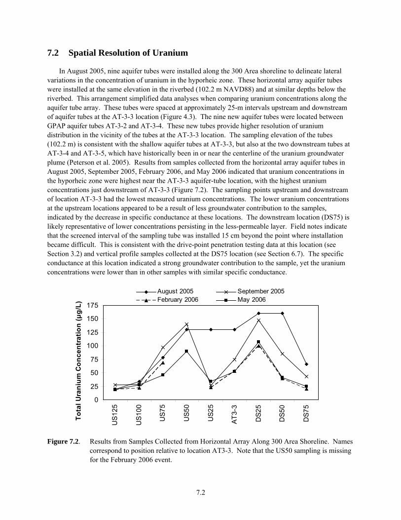
7.2

7.2 Spatial Resolution of Uranium

In August 2005, nine aquifer tubes were installed along the 300 Area shoreline to delineate lateral variations in the concentration of uranium in the hyporheic zone. These horizontal array aquifer tubes were installed at the same elevation in the riverbed (102.2 m NAVD88) and at similar depths below the riverbed. This arrangement simplified data analyses when comparing uranium concentrations along the aquifer tube array. These tubes were spaced at approximately 25-m intervals upstream and downstream of aquifer tubes at the AT-3-3 location (Figure 4.3). The nine new aquifer tubes were located between GPAP aquifer tubes AT-3-2 and AT-3-4. These new tubes provide higher resolution of uranium distribution in the vicinity of the tubes at the AT-3-3 location. The sampling elevation of the tubes (102.2 m) is consistent with the shallow aquifer tubes at AT-3-3, but also at the two downstream tubes at AT-3-4 and AT-3-5, which have historically been in or near the centerline of the uranium groundwater plume (Peterson et al. 2005). Results from samples collected from the horizontal array aquifer tubes in August 2005, September 2005, February 2006, and May 2006 indicated that uranium concentrations in the hyporheic zone were highest near the AT-3-3 aquifer-tube location, with the highest uranium concentrations just downstream of AT-3-3 (Figure 7.2). The sampling points upstream and downstream of location AT-3-3 had the lowest measured uranium concentrations. The lower uranium concentrations at the upstream locations appeared to be a result of less groundwater contribution to the samples, indicated by the decrease in specific conductance at these locations. The downstream location (DS75) is likely representative of lower concentrations persisting in the less-permeable layer. Field notes indicate that the screened interval of the sampling tube was installed 15 cm beyond the point where installation became difficult. This is consistent with the drive-point penetration testing data at this location (see Section 3.2) and vertical profile samples collected at the DS75 location (see Section 6.7). The specific conductance at this location indicated a strong groundwater contribution to the sample, yet the uranium concentrations were lower than in other samples with similar specific conductance.

0

25

50

75

100

125

150

175

US1

25

US1

00

US7

5

US5

0

US2

5

AT3-

3

DS2

5

DS5

0

DS7

5

Tota

l Ura

nium

Con

cent

ratio

n (μ

g/L)

August 2005 September 2005February 2006 May 2006

Figure 7.2. Results from Samples Collected from Horizontal Array Along 300 Area Shoreline. Names correspond to position relative to location AT3-3. Note that the US50 sampling is missing for the February 2006 event.

7.3

Other data collected in August 2005 show the spatial extent of the uranium contamination plume into the Columbia River in the hyporheic zone (i.e., the distance under the river that the uranium contaminated groundwater extends). Aquifer tubes AT-3-3M, AT3-3A.410, AT3-3B.376, and AT3-3C.409 extend into the river 15 m on a transect, roughly normal to the flow direction of the river (see Figure 4.1). All sam-pling locations have screened intervals at similar elevations (Table 7.1). All four sampling locations are near, but above the impenetrable layer observed at this location (approximately 99 m [see Section 3.2]). During the sampling event on August 29, 2005, samples from all four tubes had similar concentrations of total uranium, indicating little to no dilution from river water (Figure 7.3). This indicates that during periods of low stage, relatively undiluted groundwater can extend a considerable distance into the river channel in the hyporheic zone. Similarly, a sample collected from AT3-3C.409 in February 2006, as part of the horizontal array sampling, had a measured uranium concentration of 117 μg/L.

Table 7.1. Results from Samples Collected in August 2005 from River Tubes and Aquifer Tubes That Extend into the River at a Similar Elevation at AT-3-3

Location Elevation at Middle of Screened Interval (m)


Total Uranium Concentration

(μg/L)

AT-3-3M(a) 100.5 378 140 AT3-3A.410(b) 100 357 130 AT3-3B.376(b) 99.7 316 120 AT3-3C.409(a) 99.2 355 130 (a) Aquifer tube, 46-cm screen length. (b) River tube, 15-cm screen length.

90

95

100

105

110

115

594475 594495 594515 594535 594555 594575 594595 594615

Easting (m, State Plane, Wa South)

Elev

atio

n (m

, NAV

D88)

Avg. River Stage

River Bed

Top of Ringold Fm .

Sam pling Locations- value is uranium concentration (ug/L)

140 130 120130

Figure 7.3. Uranium Concentrations Measured in Samples Collected in August 2005 from River Tubes and Aquifer Tubes Extending into the River Channel (AT-3-3M, AT3-3A.410, AT3-3B.376, and AT3-3C.409)

7.4

7.3 Uranium Uptake in Clams

Two studies were conducted under this project to evaluate clams as a potential indicator species for areas of elevated contamination in the hyporheic zone. For the first study, these clams were split into three groups and exposed to water of varying contaminant concentrations (nominal concentrations of 4, 10, and 100 μg/L of uranium, respectively). Uranium concentrations in the clam soft tissue were measured after various exposure and depuration periods (Section 2.9). In the 100-μg/L test group, the uptake by the clams reduced the uranium concentration in the water by 40% during the 144-hour exposure period. In the second test, the initial uranium concentration in the water was lower than in the first test, but was maintained at a more uniform concentration throughout the study. Also for the second test, the initial clam concentrations were higher than the concentrations measured at the end of the uptake portion of the first 10-μg/L test (Figure 7.4). The end result of this test was that there was no observable uranium uptake in clams during the lower concentration exposures of the second test. Presumably, this was because the uranium concentration in water was less than the clams had been exposed to at the upstream reference location where the clams were collected.

The results of the first test showed that an apparent equilibrium of the uranium in clam soft tissue and water occurred within 48 hours. The second test supported this, with the concentration in clam soft tissue reaching 88% of the equilibrium concentration within 48 hours (Figure 7.4A). The results of both high concentration tests indicated that uranium was not strongly retained in the soft tissue, with clam soft tissue uranium concentrations decreasing to approximately two times the original, pre-exposure concen-tration after being exposed to low concentration water for 120+ hours. Both tests indicated that the rates at which uranium exchanges between the clam soft tissue and the water is faster than previously expected (Figure 7.4).

The ramifications of these initial uptake studies are significant. These studies indicate that contam-inants in clam soft tissue only provide an indication of short-term exposure, not long-term exposure. Making assumptions about the long-term average uranium concentration of water to which a clam has been exposed based on the uranium concentration in soft tissue would appear to be a very poor assumption at this point. Additional information on the uptake and depuration of uranium by clams is necessary to fully understand how to interpret the meaning of uranium concentrations in clam soft tissue. If water levels are changing in the Columbia River and influencing the flux of uranium-contaminated groundwater into the river substrate, clams collected from the river bottom on different days may not be comparable, and even clams collected at different times on the same day from the same location could exhibit significant differences in concentration. More research is needed to better characterize the uptake and depuration of uranium in clam soft tissue. Further tests with uranium and clam soft tissue should also evaluate the utility of using clam shells to assess long-term uranium exposure.

7.5

0

20

40

60

80

100

120

0 100 200 300 400

Hour of Test

Wat

er U

rani

um

conc

entra

tion

(μg/

L)

0.2

0.5

0.8

1.1

1.4

1.7

2.0

Cla

m U

rani

um

conc

netra

tion

(μg/

g)

WaterClams

A

0

2

4

6

8

10

12

14

16

0 100 200 300 400

Hour of Test

Wat

er U

rani

um

conc

entra

tion

(μg/

L)

0.0

0.1

0.2

0.3

0.4

0.5

0.6

0.7

0.8

Cla

m U

rani

um

conc

netra

tion

(μg/

g)

WaterClams

B

Figure 7.4. Concentrations of Uranium in Water and Clam Soft Tissue During Uptake (first 144 hours) and Depuration (next 120 hours) for Nominal Water Concentrations of 100 (A) and 10 (B) μg/L. Dashed line is second set of tests. Error bars shown for 100-μg/L test repre-sent 1 standard deviation of the average. Control test (4-μg/L water exposure) not shown.

7.4 Groundwater Level Monitoring Network in Upland Wells

To support the 300 Area modeling efforts, continuous water-level monitoring of 300 Area ground-water monitoring wells (Table 7.2) was initiated in 2004. Water-level monitoring data can be used to refine aquifer parameters and allow calibration of the three-dimensional groundwater model. Continuous water-level data for the wells and dates are listed in Table 7.2. Data were recorded at 15-minute intervals. Specific conductance and temperature were logged in six of the wells. Water-level elevations are shown superimposed on river stages for three of the wells closest to the shore near Spring 9 (Figure 7.1). The water-level, conductance, and temperature data have been provided to groups working on characterizing river stage effects on groundwater flow and reactive transport of uranium. In particular, the 2004–2005 water-level data will be used for testing and refining the simulations of flow and transport in the 300 Area

7.6

vadose zone, aquifer, and river reported by Waichler and Yabusaki (2005), which were developed using hourly river stages from the SWS-1 monitor and hourly water levels logged at 300 Area wells (see Figure 4.1).

Table 7.2. List of 300 Area Near-Shore Groundwater Wells with Continuous Level, Temperature, and Specific Conductance Monitoring, and Periods with Available Data

Well ID Data Start(a) Comment

399-1-1 07/18/2004 No data for 11/04/2004 through 12/20/2004 399-102 09/02/2004 Data available for entire period 399-1-7 08/05/2004 Specific conductance and temperature recorded 08/05/2004 - 02/17/2005

07/27/2004 399-1-12 03/02/2005

4-month gap in monitoring with brief start in March 2005

399-1-13A 07/20/2004 No data for 08/26/2004 through 09/16/2004 399-1-21A 07/28/2004 Data available for entire period 399-2-1 07/26/2004 No data for 11/04/2004 through 12/21/2004 399-2-2 07/26/2004 No data for 11/10/2004 through 12/01/2004 399-2-3 08/10/2004 Data available for entire period (a) Monitoring is ongoing in most of these wells.

Data provided by this water-level monitoring network illustrates several key points about the water table in the 300 Area. A 2-week time period is used in Figure 7.1 to illustrate these points. First, the water table near the Columbia River (well 399-2-1, approximately 50 m inland from the river edge) changes very rapidly with changing river stages, but the magnitude of the fluctuations is damped relative to the river. At a distance of 300 m inland from the river edge (well 399-1-21A), the water table changes according to daily changes in river stages, but the hourly fluctuations of the river are not observed. At a distance of 500 m inland from the river edge (well 399-1-13), the water table changes in a similar manner as observed 300 m inland, but is consistently about 0.25 m higher in elevation. This indicates that during this time period, the average water table sloped down toward the river. An important aspect of these data is that while the average gradient is toward the river, there are many time periods where the gradient near the river is from the river into the aquifer. These time periods occur when the river elevation increases above the elevation of the near-shore aquifer (Figure 7.5).

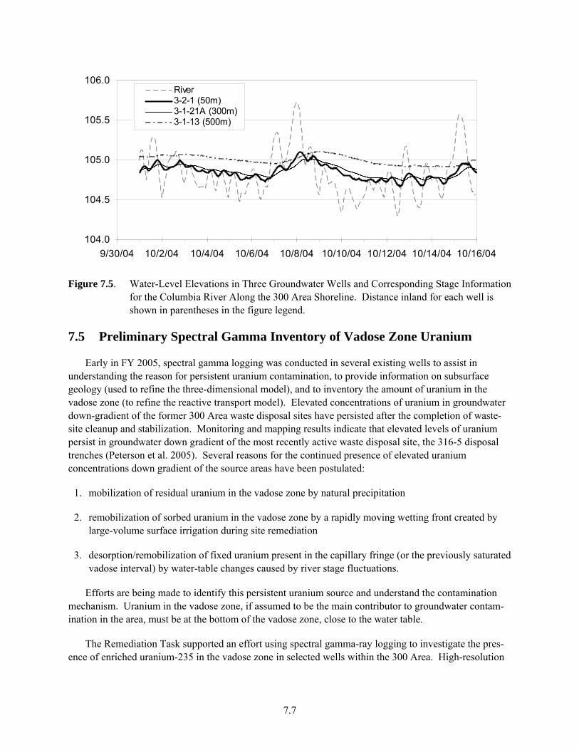
7.7

104.0

104.5

105.0

105.5

106.0

9/30/04 10/2/04 10/4/04 10/6/04 10/8/04 10/10/04 10/12/04 10/14/04 10/16/04

River3-2-1 (50m)3-1-21A (300m)3-1-13 (500m)

Figure 7.5. Water-Level Elevations in Three Groundwater Wells and Corresponding Stage Information for the Columbia River Along the 300 Area Shoreline. Distance inland for each well is shown in parentheses in the figure legend.

7.5 Preliminary Spectral Gamma Inventory of Vadose Zone Uranium

Early in FY 2005, spectral gamma logging was conducted in several existing wells to assist in understanding the reason for persistent uranium contamination, to provide information on subsurface geology (used to refine the three-dimensional model), and to inventory the amount of uranium in the vadose zone (to refine the reactive transport model). Elevated concentrations of uranium in groundwater down-gradient of the former 300 Area waste disposal sites have persisted after the completion of waste-site cleanup and stabilization. Monitoring and mapping results indicate that elevated levels of uranium persist in groundwater down gradient of the most recently active waste disposal site, the 316-5 disposal trenches (Peterson et al. 2005). Several reasons for the continued presence of elevated uranium concentrations down gradient of the source areas have been postulated:

1. mobilization of residual uranium in the vadose zone by natural precipitation

2. remobilization of sorbed uranium in the vadose zone by a rapidly moving wetting front created by large-volume surface irrigation during site remediation

3. desorption/remobilization of fixed uranium present in the capillary fringe (or the previously saturated vadose interval) by water-table changes caused by river stage fluctuations.

Efforts are being made to identify this persistent uranium source and understand the contamination mechanism. Uranium in the vadose zone, if assumed to be the main contributor to groundwater contam-ination in the area, must be at the bottom of the vadose zone, close to the water table.

The Remediation Task supported an effort using spectral gamma-ray logging to investigate the pres-ence of enriched uranium-235 in the vadose zone in selected wells within the 300 Area. High-resolution

7.8

spectral gamma logging can be used to identify the various uranium (and other gamma-emitting) isotopes in the subsurface (Figure 7.6), and monitor the associated vertical distribution.

Figure 7.6. Example of High-Resolution Gamma Logging in a Hanford Site Groundwater Monitoring Well

Five existing groundwater monitoring wells were selected for spectral gamma logging from a network of over 85 wells within the 300 Area. Well-selection criteria included the following:

• spatial location of the well relative to the high concentration areas of the uranium plume

• spatial location of the well relative to former waste disposal sites

• practicality of logging within the well based on a review of as-built diagrams

• potential for minimum gamma-signal interference from well construction materials (e.g., bentonite well seals and double strings of casing).

The wells were logged with the spectral gamma logging system (SGLS) operated by S.M. Stoller Corporation (Richland, Washington) during November 2004. The spectral data were evaluated by Stoller engineers, and the results provided to PNNL on December 2, 2004. Table 7.3 summarizes the logging results for the five wells.

Based on interpretations by Stoller, only wells 399-2-1 and 399-2-2 were identified to contain enriched uranium-235. The concentrations in these two wells were very low and bordered around the minimum detectable level (MDL). However, repeat detections of uranium-235 and the detection of other associated isotopes, uranium-238 and protactinium-234m, in these same intervals suggests the uranium-235 detections were real and not statistical noise. The uranium-235 detected in these two wells is closely associated with the water table and could reflect uranium-235 in groundwater and/or on the inside of the casing rather than in the sediments behind the casing. However, it is not possible to determine whether the uranium-235 is sorbed onto the inside of the casing or outside the casing in

7.9

formation sediment. Of particular import is that these two wells are up-gradient of the contamination plume centerline identified at the AT-3-3 aquifer tube cluster.

Table 7.3. Results of Spectral Gamma Logging at Five 300 Area Wells, November 2004. Original data collected in English units. For conversion, 1 ft = 0.3048 m.

Well Number

Water Level (depth below surface, ft)

Log Interval (repeat interval) (ft)

Enriched Uranium Detected

Isotopes Identified (feet below surface)

Concentration (pCi/g)

35.5-18.5 399-1-1 34.6

(33.5-22.5)

No 137Cs (32.5) 0.13 (MDL)

37.0-19.0 399-1-11 36

(35.0-25.0)

No 137Cs (21, 24) 0.1 (MDL)

37.0-21.0 235U (33) 235U 0.6 (MDL)

(33.0-23.0) 234mPa (22, 23, 27) 234mPa (MDL)

399-1-17A 36.2

No

137Cs (24, 26, 31) 137Cs 0.1 (MDL)

35.0-10.0 Yes 235U (17, 24, 32- 35) [29, 30, 31](a)

235U 1(b)

(35.0-25.0) U235 238U (32, 33, 34, 35) 238U

399-2-1 33.75

234mPa (28, 33, 35) 234m Pa

36.5-19.5 Yes 235U (33, 36)a 235 U 9-10 (MDL), 1(b)

399-2-2 35.7

(36.5-26.5) U235 238U (33.5, 34.5, 35.5) 238U (MDL)

MDL = Minimum detectable level. (a) Identified in repeat log. (b) Calculated concentration assumes uranium-235 is in sediment/groundwater outside of well casing, and value is

overestimated if uranium-235 is inside the casing.

One of several recommendations resulting from this work is to utilize high-resolution gamma spectral logging through cone-penetrometer boreholes to minimize gamma attenuation caused by downhole artifacts (e.g., grout seals, metal screens). This recommendation was initially incorporated into the monitoring plan for a limited-field investigation of the 300-FF-5 Operable Unit that occurred in FY 2006. In the limited-field investigation, two deep characterization boreholes were installed, and two additional wells were installed to the top of the confining layer (Williams et al. 2007). Extensive sediment sampling, hydraulic testing, and geophysical analyses were conducted to provide a more complete understanding of the geology in the 300 Area. Based on the data collected as part of the limited-field investigation, the spectral gamma logging in cone-penetrometer boreholes was deemed an inappropriate approach.

8.1

8.0 300 Area Near-Shore Monitoring Network Discussion

A number of significant accomplishments were made under this project toward evaluating and under-standing the hyporheic zone between the groundwater and Columbia River water along the 300 Area shoreline. This section is an attempt to combine and present the data from previous sections of this report into a simplified synopsis that conveys the improved understanding of uranium transport near the river, which was developed by this work.

8.1 Effect of Geology

To date, the data collected have demonstrated the necessity of a thorough understanding of the geology of the hyporheic zone to properly interpret results. Currently, evidence exists that a relatively resistant layer underlies the uppermost hydrologic unit along the shoreline in the 300 Area, and this layer limits vertical migration of contamination. Identifying the confining layer is critical in estimating uranium distribution within the hyporheic zone. The shape of the underlying confining layer may influence the contours of contaminant discharge along the shoreline. This layer is variable in elevation. These findings are supported by analytical results for aquifer tubes installed below the contact with this layer. The aquifer tube AT-3-3D (completed below the contact) consistently had measured uranium and tritium concentrations similar to Columbia River water, but had specific conductance measurements higher than river water, pH values lower than river water, and consistent temperatures of about 20°C. These data demonstrate that the water sampled from AT-3-3D was groundwater that contained low contaminant concentrations. In addition, some differences were apparent in trace-metal concentrations, which might indicate a difference in geologic origin between the uppermost hydraulic unit and the layer where the AT-3-3D aquifer tube is installed. The combination of water sampling data and drive-point penetration testing data indicate the presence of a bottom layer to the hyporheic zone that exists between 97- and 100-m elevations (NAVD88) at the AT-3-3 location. This layer limits the vertical distribution of contaminants. Indications are also present that the confining layer is deeper at the AT-3-3 location than upstream or downstream along the shoreline. A similar result measured in the aquifer tube DS75-319cm was observed. This location was installed below the suspected confining layer at Spring 10. Uranium concentrations measured at this location in September 2006 were 10 times lower than concentrations measured above the layer at the same time. These results are consistent with water samples collected as part of the limited field investigation of the 300-FF-5 Operable Unit (Williams et al. 2007). In that report, uranium concentrations decreased to undetectable concentrations below the uppermost hydraulic unit.

The geologic interpretation of the Ringold Formation (Williams et al. 2007), coupled with the high-resolution bathymetry image of the Columbia River, allows for an estimate of the area of riverbed that has the potential to discharge uranium to the Columbia River. This was done by defining an area that was 1) between the average river stage elevation (105 m) and the thalweg (deepest part) of the river, 2) between the 30 µg/L concentration contours, and 3) was not the Ringold Formation. The geologic interpretation developed for Williams et al. (2007) was used to define the top of the Ringold Formation. This approach estimated 170,000 m2 of riverbed with the potential for uranium discharge. This area is likely overestimated, as the near shore geology identified the top of Ringold Formation at slightly higher elevations than mapped by Williams et al. (2007) (Figure 3.3).

8.2

Figure 8.1. Map of Riverbed Area with the Potential to Discharge Uranium into the Columbia River. This area is between 105 m in elevation and the river thalweg, between the 30-µg/L uranium concentration contour lines onshore, and above the projected Ringold Formation.

8.2 Hyporheic Zone Response to Changing River Stage

Columbia River water levels can change by a meter or more within several hours. Several techniques were used to evaluate the response of the hyporheic zone to changing river stages. Major sampling events were scheduled to characterize the effect of different seasonal river stages in the hyporheic zone. Data logging in river tubes and near-shore groundwater wells provided a characterization of water levels, temperature, and specific conductance on a sub-hour frequency. Finally, high-frequency sampling events were conducted to evaluate other parameters beside temperature and specific conductance on an hourly time scale.

8.3

8.2.1 Example Case—October 2004

On October 9, 2004, the Columbia River level in the 300 Area dropped below 105 m in elevation. Over the ensuing week, the river elevation varied between 104.3 and 105.6 m (NAVD88). During this period of low, fluctuating river levels, a high-frequency water sampling event was conducted with hourly samples collected from the river tube SP9A.86. In addition to these water samples, the near-shore wells and river tube leveloggers recorded pressure, temperature, and specific conductance. Between October 9, 2004, and October 12, 2004, the water-level elevation in the onshore well (399-2-2) was higher than the river elevation. During this time period, the water level in the well dropped steadily, indicating that the aquifer was draining into the river. This was supported by the measured specific conductance in the river tube, which steadily increased until the river elevation was higher than the water elevation in the well (Figure 8.1). When the river elevation increased above the water elevation in the nearest well, the specific conductance and the water level in the well began to increase. This demonstrated a change in direction of water movement in the hyporheic zone and resulted in river water moving into the aquifer. The decrease in specific conductance values in the river tube continued until the river elevation again dropped below the water table elevation in the near-shore aquifer. At this point, the specific conductance in the river tubes began to increase, and the water level in the aquifer began to decrease. This pattern continued through the sampling event, which ended on October 15.

0

50

100

150

200

250

300

350

400

450

500

8-Oct 9-Oct 10-Oct 11-Oct 12-Oct 13-Oct 14-Oct 15-Oct 16-Oct 17-Oct

Spec

ific

Con

duct

ance

(μS/

cm)

104.0

104.2

104.4

104.6

104.8

105.0

105.2

105.4

105.6

105.8

106.0

Wat

er E

leva

tion

(m)

Sp. Cond. River elevation (m) WL Elevation 399-2-2 (m)

Figure 8.2. Specific Conductance (SC) Results from High-Frequency Sampling Event at AT3-3-124 in October 2004, and Corresponding Water Elevations of River and Nearest Onshore Groundwater Well (399-2-2)

Columbia River levels influenced the direction of water movement in the hyporheic zone, and were clearly demonstrated by the changes in specific conductance measured in the river tubes. Changes in the hydraulic gradient measured at the riverbed and in the hyporheic zone also quantified river stage change effects. For the October 2004 example, data from a levelogger in SP9A-86 and one on the riverbed was converted to hydraulic gradient. The direction and magnitude of the vertical hydraulic gradient measured in the river tube is clearly a function of the difference between river elevation and the water-level elevation in the nearest well. When the river elevation increased above the water elevation in the well, the measured hydraulic gradient was into the riverbed (positive is defined as out of the riverbed). When

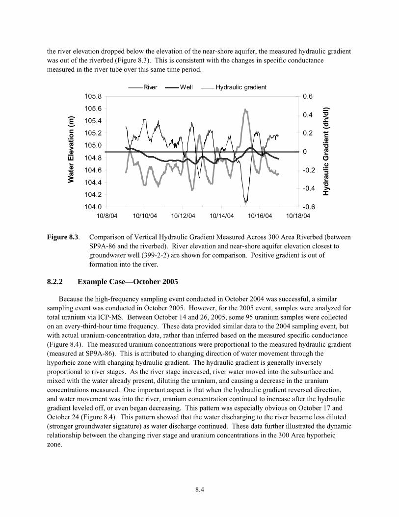
8.4

the river elevation dropped below the elevation of the near-shore aquifer, the measured hydraulic gradient was out of the riverbed (Figure 8.3). This is consistent with the changes in specific conductance measured in the river tube over this same time period.

104.0

104.2

104.4

104.6

104.8

105.0

105.2

105.4

105.6

105.8

10/8/04 10/10/04 10/12/04 10/14/04 10/16/04 10/18/04

Wat

er E

leva

tion

(m)

-0.6

-0.4

-0.2

0

0.2

0.4

0.6

Hyd

raul

ic G

radi

ent (

dh/d

l)

River Well Hydraulic gradient

Figure 8.3. Comparison of Vertical Hydraulic Gradient Measured Across 300 Area Riverbed (between SP9A-86 and the riverbed). River elevation and near-shore aquifer elevation closest to groundwater well (399-2-2) are shown for comparison. Positive gradient is out of formation into the river.

8.2.2 Example Case—October 2005

Because the high-frequency sampling event conducted in October 2004 was successful, a similar sampling event was conducted in October 2005. However, for the 2005 event, samples were analyzed for total uranium via ICP-MS. Between October 14 and 26, 2005, some 95 uranium samples were collected on an every-third-hour time frequency. These data provided similar data to the 2004 sampling event, but with actual uranium-concentration data, rather than inferred based on the measured specific conductance (Figure 8.4). The measured uranium concentrations were proportional to the measured hydraulic gradient (measured at SP9A-86). This is attributed to changing direction of water movement through the hyporheic zone with changing hydraulic gradient. The hydraulic gradient is generally inversely proportional to river stages. As the river stage increased, river water moved into the subsurface and mixed with the water already present, diluting the uranium, and causing a decrease in the uranium concentrations measured. One important aspect is that when the hydraulic gradient reversed direction, and water movement was into the river, uranium concentration continued to increase after the hydraulic gradient leveled off, or even began decreasing. This pattern was especially obvious on October 17 and October 24 (Figure 8.4). This pattern showed that the water discharging to the river became less diluted (stronger groundwater signature) as water discharge continued. These data further illustrated the dynamic relationship between the changing river stage and uranium concentrations in the 300 Area hyporheic zone.

8.5

0

20

40

60

80

100

120

140

160

10/14/05 10/17/05 10/20/05 10/23/05 10/26/05

Ura

nium

Con

cent

ratio

n (u

g/L)

-0.8

-0.6

-0.4

-0.2

0.0

0.2

0.4

0.6

0.8

Verti

cal H

ydra

ulic

Gra

dien

t

Uranium Concentration hydraulic gradient

Figure 8.4. Fluctuating Uranium Concentrations Measured in the Hyporheic Zone. Concentrations changed with the measured hydraulic gradient.

8.2.3 Uranium Discharge

Total uranium discharge into the Columbia River from the 300-FF-5 unit was previously reported to be 430 kg per year (DOE 1994). The head elevation and specific conductance data collected within the hyporheic zone by this project was used to develop a detailed evaluation of both water and uranium flux through the hyporheic zone. The analysis of that data is published in Fritz and Arntzen (2007), and is not replicated in this report. The results provided an estimate of an annual uranium flux of 2.25 μg/min/m2. When combined with the estimated potential uranium discharge area (170,000 m2, Figure 8.1), the total annual uranium discharge to the Columbia River was estimated to be 200 kg/year. This value may be an overestimate of the total uranium discharge to the Columbia River because the flux estimate is from the center of the uranium plume, and the total potential area for discharge is likely overestimated (based on near shore geology data). This uranium discharge estimate can be put into context by a comparison to other uranium sources along the Hanford Reach (Appendix B).

8.3 Evaluating Uranium Concentrations in the Biotic Zone

There is a growing interest in the biotic zone at the interface between the hyporheic zone and the Columbia River. The biotic zone is the portion of the near-shore riverbed where plants and animals can be found, and may be the location with the highest potential for impacts from uranium discharges into the Columbia River. Defining this biotic zone, and collecting samples from it, is a difficult task due to the variability in cobble size and sediment properties along the Hanford Reach. For the purposes of this report, the authors define the biotic zone as the portion of the riverbed existing between the top of the river cobble (excluding large boulders) down to a depth 10 cm below the sediment/water interface. Based on this definition, the biotic zone is between 15 and 20 cm thick in most areas along the 300 Area shoreline. The majority of GPAP and SESP environmental samples have been collected in the subsurface below the biotic zone or in the river above the biotic zone. Perhaps the best uranium exposure data for the biotic zone can be obtained from a levelogger installed on the bed of the Columbia River. This levelogger was initially deployed to provide the river elevation measurement necessary in calculating

8.6

discharges via Darcy’s Law, and was positioned as closely as possible to the sediment/water interface. The levelogger also recorded specific-conductance measurements. Thus, using the relationship between specific conductance and uranium concentration (see Section 6.7), the uranium concentration at the top of the biotic zone could be estimated, although the specific conductance method was not considered applicable below 150 μS/cm (Figure 8.5). The uranium concentrations are a function of the river stage, and estimated uranium concentrations in the biotic zone exceed 120 μg/L during certain time periods. This fluctuation is consistent with concentrations measured in the subsurface during some sampling events, indicating that little or no dilution of the subsurface water occurs in the biotic zone during periods of strong discharge to the river. Additional evaluation of the uranium concentrations in the biotic zone are necessary to fully characterize the net-uranium exposure to biota resulting from the varying uranium discharges under fluctuating Columbia River levels.

0

20

40

60

80

100

120

140

8/1/20

04

9/1/20

04

10/1/

2004

11/1/

2004

12/1/

2004

1/1/20

05

2/1/20

05

3/1/20

05

4/1/20

05

5/1/20

05

6/1/20

05

7/1/20

05

8/1/20

05Estim

ated

Ura

nium

Con

cent

ratio

n (μ

g/L)

0

50

100

150

200

250

300

Wat

er D

epth

(cm

)

Estimated U (μg/L)Water depth (cm)

Figure 8.5. Estimated Uranium Concentrations in the 300 Area Biotic Zone (at the water/sediment interface) Compared to River Water Depth at the Measurement Location

9.1

9.0 Conclusions

The transport of uranium-contaminated groundwater through the hyporheic zone of the 300 Area to the Columbia River is complicated. This report provides information that assists in furthering the understanding of this dynamic system, and provides data that will be useful in making and evaluating remediation decisions. The general conclusions reached as a result of this work are listed below, the details of which can be found in the relevant sections.

9.1 Geology

• A hydrostratographic contact between two distinct geologic layers exists in the near-shore region adjacent to the 300 Area. This contact is interpreted to be the interface between the Hanford formation (river alluvium) and the Ringold Formation. This is consistent with recent geologic interpretations conducted inland of the river.

• The elevation of the Ringold contact in the near-shore region is generally consistent with the elevations mapped out inland based on well-log data.

• The Ringold contact outcrops directly in the river channel in some locations.

• The riverbed area that possesses the potential to discharge uranium to the river is estimated to be 170,000 m2.

9.2 Water Sampling

• Specific conductance was shown to be a good indicator of uranium concentration in water samples collected from the hyporheic zone at the 300 Area.

• Concentrations of most constituents measured in water in the hyporheic zone varied proportionally with specific conductance, suggesting the dilution of groundwater by river water.

• Uranium concentrations in the hyporheic zone were measured as high as 195 μg/L.

• With the methods used in this study, no evidence was presented of uranium sorption onto sediment in the hyporheic zone. The ratio of tritium to uranium in samples did not vary with specific conductance. Also, filtered/unfiltered sample pairs had similar measured-uranium concentrations. However, there were no direct measurements of uranium concentrations in sediment conducted for this project.

• The Ringold Formation appears to limit vertical movement of contamination for both tritium and uranium.

• The uranium concentration in the hyporheic zone changed very quickly in response to changing river stage, although deeper locations responded more slowly than the shallower locations.

9.2

9.3 Uranium Uptake in Clams

• The uranium concentration in clam soft tissue increases in a matter of days in response to an increase in uranium concentration in water.

• The uranium concentration in clam soft tissue decreases (at a slower rate than uptake) when the uranium concentration in water was decreased.

9.4 Continuous Monitoring

• Specific conductance, temperature, and uranium concentration change quickly in the hyporheic zone in response to changing river stage.

• As expected, the direction of the hydraulic gradient at the water-sediment interface is determined by the river elevation and the near-shore aquifer elevation.

9.5 Future Work

This report provides various data that assist in improving the understanding of the dynamic nature of uranium transport in the hyporheic zone along the shoreline of the Columbia River, adjacent to the 300 Area of the Hanford Site. Future work should primarily focus on providing data necessary for refinement of a three-dimensional computer model being developed for the 300 Area. These data could include a more detailed analysis of the bathymetric survey of the riverbed, a better depiction of the Ringold contact elevation along the Columbia River edge, and more measurements of the hydraulic properties of the hyporheic zone.

10.1

10.0 References

Alayamani MS and Z Sen. 1993. “Determination of Hydraulic Conductivity from Complete Grain-Size Distribution Curves.” Ground Water 31:551-555.

Anglin DR, SL Haeseker, JJ Skalicky, H Schaller, KF Tiffan, JR Hatten, P Hoffarth, J Nugent, D Benner, and M Yoshinaka. 2006. Effects of Hydropower Operations on Spawning Habitat, Rearing Habitat, and Stranding/Entrapment Mortality of Fall Chinook Salmon in the Hanford Reach of the Columbia River. U.S. Fish and Wildlife Service, Washington, D.C.

Arntzen EV, DR Geist, and PE Dresel. 2006. “Effects of Fluctuating River Flow on Groundwater/ Surface Water Mixing in the Hyporheic Zone of a Regulated, Large Cobble Bed River. River Research and Applications 22:1-10.

Baker VR, BN Bjornstad, AJ Busacca, KR Fecht, EP Kiver, VL Moody, JG Rigby, DF Stradling, and AM Tallman. 1991. “Quaternary Geology of the Columbia Plateau,” The Geology of North America, Vol. K-2, “Quaternary Nonglacial Geology, Conterminous United States,” Geological Society of America, Boulder, Colorado, pp. 215-250.

Bjornstad BN, KR Fecht, and CJ Pluhar. 2001. “Long History of Pre-Wisconsin, Ice Age Cataclysmic Floods: Evidence from Southeastern Washington State.” Journal of Geology 109:695-713.

Bouwer H. 1989. “The Bouwer and Rice Slug Test: An Update.” Ground Water 111:304-309.

Bouwer H and RC Rice. 1976. “A Slug Test for Determining Hydraulic Conductivity of Unconfined Aquifers with Completely or Partially Penetrating Wells.” Water Resources Research 12:423-428.

Burger RL and K Belitz. 1997. “Measurement of Anisotropic Hydraulic Conductivity in Unconsolidated Sands: A Case Study from a Shoreface Deposit, Oyster, Virginia.” Water Resources Research 33:1515-1522.

Butler JJ. 1998. The Design, Performance, and Analysis of Slug Tests. CRC Press LLC, Boca Raton, Florida.

Comprehensive, Environmental Response, Compensation, and Liability Act. 1980. Public Law 96-510, as amended, 94 Stat. 2767, 42 USC 9601 et seq.

Conyers LB and D Goodman. 1997. Ground-Penetrating Radar: An Introduction for Archaeologists. AltaMira Press, Walnut Creek, California.

Conyers LB and JE Lucius. 1996. “Velocity Analysis in Archaeological Ground-Penetrating Radar Studies.” Archaeological Prospection 3:25-38.

Davis JL and AP Annan. 1989. “Ground-Penetrating Radar for High-Resolution Mapping of Soil and Rock Stratigraphy.” Geophysics 37:531-551.

10.2

DOE. 2002. 300-FF-5 Operable Unit Sampling and Analysis Plan. DOE/RL-2002-11, Rev. 0. Prepared by CH2M HILL Hanford, Inc. for the U.S. Department of Energy, Richland Operations Office, Richland, Washington.

DOE. 1994. Phase I Remedial Investigation Report for the 300-FF-5 Operable Unit. DOE/RL-93-21, U.S. Department of Energy, Richland Operations Office, Richland, Washington.

EPA. 1983. EPA Method 310. Alkalinity in Methods for Chemical Analysis of Water and Wastes. EPA/600/4-79/020, U.S. Environmental Protection Agency, Washington, D.C.

EPA. 1994. EPA Method 200.8. Determination of Trace Elements in Waters and Wastes by Inductively Coupled Plasma-Mass Spectrometry. Rev. 5.4, U.S. Environmental Protection Agency, Washington, D.C.

EPA. 1996a. Record of Decision for USDOE Hanford 300-FF-1 and 300-FF-5 Operable Units Remedial Actions. Agreement Between U.S. Department of Energy and U.S. Environmental Protection Agency, with Concurrence by the Washington State Department of Ecology, July 17, 1996.

EPA. 1996b. EPA Methods 1638. Determination of Trace Elements in Ambient Waters by Inductively Coupled Plasma — Mass Spectrometry. U.S. Environmental Protection Agency, Washington, D.C.

EPA. 1997a. EPA Method 300.1. Methods for the Determination of Organic and Inorganic Compounds in Drinking Water, Volume 1. EPA 815-R-00-014, U.S. Environmental Protection Agency, Washington, D.C.

EPA 1997b. EPA Method 1640. Determination of Trace Elements in Water by Preconcentration and Inductively Coupled Plasma Mass Spectrometry. U.S. Environmental Protection Agency, Washington, D.C.

Fritz, BG and EV Arntzen. 2007. “Effect of Rapidly Changing River Stage on Uranium Flux Through the Hyporheic Zone.” Ground Water in press.

Gaylord DR and EP Poeter. 1991. Geology and Hydrology of the 300 Area and Vicinity, Hanford Site, South Central Washington. WHC-EP-0500, Westinghouse Hanford Company, Richland, Washington.

Geist DR. 2000. “Hyporheic Discharge of River Water into Fall Chinook Salmon (Oncorhynchus tshawytscha) Spawning Areas in the Hanford Reach, Columbia River.” Canadian Journal of Fisheries and Aquatic Sciences 57:1647-1656

Hanf RW, TM Poston, and LE Bisping. 2007. Surface Environmental Surveillance Procedures Manual PNL-MA-580, Rev. 5. PNNL-16744 (PNL-MA-580, Rev. 5), Pacific Northwest National Laboratory, Richland, Washington, as amended.

Hope SJ and RE Peterson. 1996a. Pore Water Chromium Concentration at 100-H Reactor Area Adjacent to Fall Chinook Salmon Spawning Habitat of the Hanford Reach, Columbia River. BHI-00345, Bechtel Hanford, Inc., Richland, Washington.

10.3

Hope SJ and RE Peterson. 1996b. Chromium in River Substrate Pore Water and Adjacent Groundwater: 100-D/DR Area, Hanford Site, Washington. BHI-00778, Bechtel Hanford, Inc., Richland, Washington.

Hulstrom LC. 1993. Sampling and Analysis of the 300-FF-5 Operable Unit Springs and Near Shore Sediments and River Water. WHC-SD-EN-TI-125, Westinghouse Hanford Company, Richland, Washington.

Landon MK, DL Rus, and FE Harvey. 2001. “Comparison of Instream Methods for Measuring Hydraulic Conductivity in Sandy Streambeds.” Ground Water 39:870-885.

Lee DR, DR Geist, K Saldi, D Hartwig, and T Cooper. 1997. Locating Ground-Water Discharge in the Hanford Reach of the Columbia River. PNNL-11516, Pacific Northwest National Laboratory, Richland, Washington.

Lindsey KA. 1995. Miocene- to Pliocene-Aged Suprabasalt Sediments of the Hanford Site, South-Central Washington. BHI-00184, Rev. 0., Bechtel Hanford, Inc., Richland, Washington.

Lindberg JW and FW Bond. 1979. Geohydrology and Ground-Water Quality Beneath the 300 Area, Hanford Site, Washington. PNL-2949, Pacific Northwest Laboratory, Richland, Washington.

Lucius JE, RJ Horton, MH Powers, and LB Conyers. 1998. Multidisciplinary Approach to Interpreting GPR at the Ceren Archaeological Site, El Salvador. Paper presented at the proceedings of the 7th International Conference on Ground Penetrating Radar, Lawrence, Kansas.

NAVD88. 1988. North American Vertical Datum of 1988.

Patton GP, BL Tiller, EJ Antonio, TM Poston, and SP Van Verst. 2003. Survey of Radiological and Chemical Contaminants in the Near-Shore Environment at the Hanford Site 300 Area. PNNL-13692, Rev. 1, Pacific Northwest National Laboratory, Richland, Washington.

Peterson RE, EJ Freeman, PD Thorne, MD Williams, JL Lindberg, CJ Murray, MJ Truex, SB Yabusaki, JP McDonald, VR Vermeul, and JM Zachara. 2005. Contaminants of Potential Concern in the 300-FF-5 Operable Unit: Expanded Annual Groundwater Report for Fiscal Year 2004. PNNL 15127, Pacific Northwest National Laboratory, Richland, Washington.

Peterson RE and MP Connelly. 2001. Zone of Interaction Between Hanford Site Groundwater and Adjacent Columbia River. PNNL-13674, Pacific Northwest National Laboratory, Richland, Washington.

Peterson RE, JV Borghese, and DB Erb. 1998. Aquifer Sampling Tube Completion Report: 100 Area and Hanford Townsite Shorelines. BHI-01153, Bechtel Hanford, Inc., Richland, Washington.

Poston TM, RW Hanf, RL Dirkes, and LF Morasch. 2004. Hanford Site Environmental Report for Calendar Year 2003. PNNL-14687, Pacific Northwest National Laboratory, Richland, Washington.

Powers MH. 1995. Dispersive Ground Penetrating Radar Modeling in 2D. Doctoral dissertation, Colorado School of Mines, Golden, Colorado.

10.4

Resource Conservation and Recovery Act. 1976. Public Law 94-580, as amended, 90 Stat. 2795, 42 USC 6901 et seq.

Schalla RR, W Wallace, RL Aaberg, SP Airhart, DJ Bates, JVM Carlile, CS Cline, DI Dennison, MD Freshley, PR Heller, EJ Jensen, KB Olsen, RG Parkhurst, JT Rieger, and EJ Westergard. 1988. Interim Characterization Report for the 300 Area Process Trenches. PNL-6716, Pacific Northwest Laboratory, Richland, Washington.

Sellman PV, SA Arcone, and AJ Delaney. 1983. Radar Profiling of Buried Reflectors and the Ground Water Table. Issue Brief No. 83:11, 1-10, Cold Regions Research and Engineering Laboratory Report, Hanover, New Hampshire.

Swanson LC. 1992. Phase I Hydrogeologic Summary of the 300-FF-5 Operable Unit, 300 Area. WHC-SD-EN-TI-052, Westinghouse Hanford Company, Richland, Washington.

Thorne PD, MA Chamness, FA Spane, VR Vermeul, and WB Webber. 1993. Three-Dimensional Conceptual Model for the Hanford Site Unconfined Aquifer System, FY 1993. PNL-8971, Pacific Northwest Laboratory, Richland, Washington.

USACE – U.S. Army Corps of Engineers. 2005. Water Management Web Site. Accessed October 20, 2007, at http://www.nwd-wc.usace.army.mil.

USGS – U.S. Geological Survey. 2007. Water Watch – Current Water Resources Conditions. Accessed October 20, 2007, at http://water.usgs.gov/waterwatch/?m=real&r=wa.

Vaux WG. 1968. “Intragravel Flow and Interchange of Water in a Streambed.” Fishery Bulletin 66:479-489.

Waichler SR and SB Yabusaki. 2005. Flow and Transport in the Hanford 300 Area Vadose Zone-Aquifer-River System. PNNL-15125, Pacific Northwest National Laboratory, Richland, Washington.

Weight WD and GP Wittman. 1999. “Oscillatory Slug-Test Data Sets: A Comparison of Two Methods.” Ground Water 37:827-835.

Westbrook, SJ, JL Rayner, GB Davis, TP Clement, PL Bjerg and SJ Fisher. 2005. “Interaction Between Shallow Groundwater, Saline Surface Water and Contaminant Discharge at a Seasonally and Tidally Forced Boundary.” Journal of Hydrology 302:255-269.

White DS. 1993. “Perspectives on Defining and Delineating Hyporheic Zones.” Journal of North American Benthological Society 12:61-69.

Williams BA, CF Brown, W Um, MJ Nimmons, RE Peterson, BN Bjornstad, DC Lanigan, RJ Serne, FA Spane, and ML Rockhold. 2007. Limited Field Investigation Report for Uranium Contamination in the 300 Area, 300-FF-5 Operable Unit, Hanford Site, Washington. PNNL-16435, Pacific Northwest National Laboratory, Richland, Washington.

Woessner WW. 2000. “Stream and Fluvial Plain Ground Water Interactions: Rescaling Hydrogeologic Thought.” Ground Water 38:423-429.

Appendix A

Aquifer Tube Installation Method from Geoprobe Systems®

Available online at http://www.geoprobe.com/products/tools/soil_gas/implantdesc.htm

A.1

Appendix A

Aquifer Tube Installation Method from Geoprobe Systems®

Appendix B

Comparison of Hanford Reach Uranium Contributors

B.1

Appendix B

Comparison of Hanford Reach Uranium Contributors

Uranium entering the Columbia River along the Hanford Reach comes from a variety of places, including the 300-FF-5 Operable Unit and irrigation returns along the Franklin County shoreline. Here, the authors present a scoping assessment of the relative contributions of these sources, along with a comparison to the total uranium entering the Columbia River along the Hanford Reach. The uranium concentrations reported in this report are data collected as part of the characterization of systems project, and are stored in the Hanford Environmental Information System (HEIS) database.

B.1 300-FF-5

The calculated annual mass of uranium that enters the Columbia River from the 300-FF-5 Operable Unit is a function of two measurements – the mass flux rate of uranium and the discharge area. The annual average mass flux rate was calculated from pressure and specific conductance measured at a vertical array of three piezometers installed near the centerline of the uranium groundwater contamination plume. Data collection spanned 15 months during 2004 and 2005. The annual average uranium mass-flux rate from this calculation is 2.25 μg/m2/min. The discharge area was calculated as the area between the 30 µg/L groundwater plume contours, the elevation of the uranium confining layer, the average river elevation, and the river bottom elevation over the discharge area. This area is 170,000 m2. Combining these two values results in an estimated uranium discharge to the Columbia River from the 300-FF-5 Operable Unit of 200 kg/yr.

B.2 Irrigation Returns

In 2003, water samples from three irrigation returns along the Franklin County shoreline were collected and analyzed. These canals were the Esquatzel, Ringold, and Potholes canals. The uranium-water concentrations measured in the Esquatzel, Ringold, and Potholes canals were 6 µg/L, 8.5 µg/L, and 3 µg/L, respectively. In 2003, the total volume of water dumped from these canals into the Columbia River was 1x1011, 1.1x1011, and 2.7x1010 L, respectively (data from the Bureau of Reclamation). Combining these data results in an estimated uranium input to the Columbia River for 2003: Esquatzel (600 kg/yr), Ringold (935 kg/yr), and Potholes (81 kg/yr). This assumes that the uranium concentration was constant throughout the entire year.

B.3 Total Columbia River

Continuous water sampling at an upstream location (Priest Rapids Dam) and a location downstream of the 300-FF-5 Operable Unit (Richland Pumphouse) is conducted as part of the routine Hanford Site environmental surveillance. Between 2000 and 2005, the typical difference in annual average Columbia River water uranium concentration at these two locations was 0.09 µg/L. Note that the measured upstream/downstream difference is not statistically significant, but for the sake of this analysis, it is treated as a real difference. Typical Columbia River annual water discharge from Priest Rapids Dam over this time period was 9.6 x1013 L/yr. The mass of uranium that must enter the Columbia River along the

B.2

Hanford Reach to account for the 0.09 µg/L increase in uranium concentration is then 8600 kg. More recently, in 2004 and 2005, the average difference between upstream and downstream river concen-trations of uranium has been 0.02 µg/L. This difference would require approximately 2000 kg of uranium to enter the river along the Hanford Reach each year. Based on these calculations, the 300-FF-5 Operable Unit contributes between 2% and 10% of the uranium that enters the Columbia River on an annual basis in the Hanford Reach. This is likely a conservative estimate of the total uranium entering the river, as cross-river transect sampling shows that the uranium concentrations are not well mixed at the Richland Pumphouse (the downstream sampling location), and that uranium concentrations are actually higher along the Franklin County shoreline. Therefore, the upstream and downstream measurements likely do not represent a complete mass balance for uranium in the Columbia River.

For comparison purposes, the Yakima River is estimated to contribute 4000 kg of uranium per year to the Columbia River. This is based on a 1.5 µg/L uranium concentration measured in Yakima River water, and the average annual discharge of water from the Yakima to the Columbia between 2002 and 2004 (2.6x1012 L per year). The discharge was measured at the Kiona gauging station near Benton City.

PNNL-16805

Distr 1

Distribution No. of Copies ONSITE 5 U.S. Department of Energy M. Thompson (5) A6-38 1 U.S. Environmental Protection Agency A. Boyd B1-46 3 Fluor Hanford S. W. Petersen E6-35 R. D. Mahood E6-35 J. V. Borghese E6-35

No. of Copies 31 Pacific Northwest National Laboratory E. V. Arntzen K6-85 A. L. Bunn K3-61 R. L. Dirkes K6-75 E. P. Dresel K6-96 M. D. Freshley K9-33 B. G. Fritz (10) K6-75 J. S. Fruchter K6-96 T. J. Gilmore K6-96 K. B. Larson K6-85 R. D. Mackley K6-96 D. McFarland K6-75 D. P. Mendoza K6-81 G. W. Patton K6-75 R. E. Peterson K6-75 T. M. Poston K6-75 R. M. Smith K6-96 A. Stegen K3-66 V. R. Vermeul K6-96 M. D. Williams K6-96 S. B. Yabusaki K9-36 Hanford Technical Library (2) P8-55

investigation of the hyporheic zone at the 300 area ... · disclaimer this report was prepared as...

Documents