investigation of the response of groups of wave …
TRANSCRIPT
INVESTIGATION OF THE RESPONSE OF GROUPS OF WAVE
ENERGY DEVICES
A thesis submitted to the University of Manchester for the degree of
Doctor of Philosophy
in the Faculty of Engineering and Physical Sciences
2011
Sarah Bellew1
School of Mechanical, Aerospace and Civil Engineering
1nee Thomas

Contents
Nomenclature 5
Abstract 12
Lay Abstract 13
Declaration 14
Copyright Statement 15
Acknowledgement 16
The Author 17
1 Introduction 18
1.1 The Current Stage of the Industry . . . . . . . . . . . . . . . . . . . . 18
1.2 Closely Spaced Arrays . . . . . . . . . . . . . . . . . . . . . . . . . . . 23
1.3 Design Challenges for Wave Energy Devices . . . . . . . . . . . . . . . 24
1.4 Research and Development Methods . . . . . . . . . . . . . . . . . . . 25
1.5 Modelling Real Sea States . . . . . . . . . . . . . . . . . . . . . . . . . 26
1.6 Hydrodynamic Modelling Techniques . . . . . . . . . . . . . . . . . . . 27
1.7 Synopsis . . . . . . . . . . . . . . . . . . . . . . . . . . . . . . . . . . 32
2 Linear Modelling of an Array 34
2.1 Modelling the Fluid . . . . . . . . . . . . . . . . . . . . . . . . . . . . 34
2.2 Modelling Wave Energy Converters . . . . . . . . . . . . . . . . . . . . 42
2.3 Parameters . . . . . . . . . . . . . . . . . . . . . . . . . . . . . . . . . 45
2.4 Calculating Body Forces . . . . . . . . . . . . . . . . . . . . . . . . . . 46
2.5 Power . . . . . . . . . . . . . . . . . . . . . . . . . . . . . . . . . . . . 51
2.6 Interaction Factors . . . . . . . . . . . . . . . . . . . . . . . . . . . . . 54
2.7 Chapter Summary . . . . . . . . . . . . . . . . . . . . . . . . . . . . . 58
2

3 Comparison to Experiment 60
3.1 Introduction . . . . . . . . . . . . . . . . . . . . . . . . . . . . . . . . 60
3.2 Experimental Set-Up and Measured Response . . . . . . . . . . . . . . 62
3.3 Numerical Prediction of Response . . . . . . . . . . . . . . . . . . . . . 63
3.4 Statistical Comparison of Methods . . . . . . . . . . . . . . . . . . . . 70
3.5 Discussion of Model Discrepancies . . . . . . . . . . . . . . . . . . . . 75
3.6 Chapter Conclusion . . . . . . . . . . . . . . . . . . . . . . . . . . . . . 81
4 Second Order Forcing 83
4.1 Second Order Solution Methods . . . . . . . . . . . . . . . . . . . . . 84
4.2 Second Order Effects . . . . . . . . . . . . . . . . . . . . . . . . . . . . 86
4.3 Sea State Description . . . . . . . . . . . . . . . . . . . . . . . . . . . 88
4.4 Calculating Dimensionalised Forces . . . . . . . . . . . . . . . . . . . . 91
4.5 Interpolation . . . . . . . . . . . . . . . . . . . . . . . . . . . . . . . . 94
4.6 Variation of Forces with Hs and Tp . . . . . . . . . . . . . . . . . . . . 100
4.7 Chapter Conclusion . . . . . . . . . . . . . . . . . . . . . . . . . . . . . 108
5 Optimisation of Fixed Geometry Arrays 110
5.1 Introduction . . . . . . . . . . . . . . . . . . . . . . . . . . . . . . . . . 110
5.2 Basic Approaches to Selecting Diagonal M and R Matrices . . . . . . . 113
5.3 Diagonal Damping Matrix Selection Procedure . . . . . . . . . . . . . 119
5.4 Direct Sub-Optimal R Matrix Calculation . . . . . . . . . . . . . . . . 125
5.5 Iteratively-Selected Mechanical Damping . . . . . . . . . . . . . . . . . 127
5.6 Iteratively-Selected Mass . . . . . . . . . . . . . . . . . . . . . . . . . 136
5.7 Chapter Conclusion . . . . . . . . . . . . . . . . . . . . . . . . . . . . 138
6 Optimisation of Geometries 141
6.1 Direct Neighbour Coupling . . . . . . . . . . . . . . . . . . . . . . . . 143
6.2 Draft Variation of Isolated Body . . . . . . . . . . . . . . . . . . . . . 144
6.3 Optimal Draft: ConTop . . . . . . . . . . . . . . . . . . . . . . . . . . 151
6.4 Draft Variation Within an Array . . . . . . . . . . . . . . . . . . . . . 155
6.5 Chapter Conclusion . . . . . . . . . . . . . . . . . . . . . . . . . . . . . 162
7 Conclusion 165
7.1 Overview . . . . . . . . . . . . . . . . . . . . . . . . . . . . . . . . . . . 165
7.2 Mathematical Conclusions . . . . . . . . . . . . . . . . . . . . . . . . . 166
7.3 Engineering Conclusions . . . . . . . . . . . . . . . . . . . . . . . . . . 167
3
7.4 Future Work . . . . . . . . . . . . . . . . . . . . . . . . . . . . . . . . . 169
A Mathematical Identities 172
B Complex Amplitudes 174
C Defining Geometries in WAMIT 176
D Analytical Froude-Krylov Force 178
E Numerical Froude-Krylov Force 180
F Derivation of the Full Power Equation 182
G Statistical Measures 184
H Geometry Specifications of ConTop 188
I Variation of Hydrodynamic Parameters with Float Draft 191
J Relationship Between Response and Power 200
Word Count: 64 468
4
Nomenclature
A Added Mass, page 44
Am Wave Amplitude, page 38
ACsZ Cross-sectional area of the float in the vertical plane perpendicular to the
direction of wave propagation , page 76
AWP Water-plane area, page 64
Aϑ Added mass which would be experienced after a phase shift, page 79
B Radiation damping, page 44
Bϑ Radiation damping which would be experienced after a phase shift, page 79
C Restoring coefficient, page 43
Cd Drag coefficient, page 76
Cg Group velocity, page 77
Cz A set of terms used in the derivation of Equation (2.49), page 183
D5 5 m Vertical circular cylinder draft, page 155
D% The difference between the interaction factor for an array with R selected
iteratively and an array with R = diag(Ropt), page 129
D10 10 m Vertical circular cylinder draft, page 155
D15 15 m Vertical circular cylinder draft, page 155
F Excitation Force (simplified notation for Fe), page 46
F [1] Dimensional first-order excitation force, page 91
F[2]+ Dimensional second-order excitation force at sum frequency, page 92
5
F[2]− Dimensional second-order excitation force at difference frequency, page 92
FD The total damping on an array of floats such that FD = R +B, page 158
Fe Excitation force, page 43
Fr Radiation force, page 43
Ft Time series of dimensional forces, page 92
Fdamp Mechanical damping force, page 43
Fext External driving force, page 43
Ffd Viscous drag, page 76
Fres Restoring force, page 43
G(t) Arbitrary function of time only, page 36
G (θ, ψi) Function used to simplify Equation (2.45), page 50
H Wave height, page 23
H1 Initial height of radiated wave, page 78
H2 Height of radiated wave at the channel wall, page 78
H3 Height of wave at body centre after being radiated and reflected back from
channel wall, page 78
Hs Significant wave height, page 89
L Wavelength, page 24
M Body (dry) mass, page 43
Mm The displaced mass of a float, page 62
Msup Supplementary mass on float, page 62
N Number of bodies, page 34
NR Number of damping values considered in Method 1, page 120
P Power, page 52
P0 Power from an isolated device, page 110
6

P1(ω) The maximum net power from the coarse net power range for which R
values are determined during the iterative procedure of Method 2, page 122
Pc Power in an arc of a circular wave radiated from a body, page 77
Pw Power per unite length of wave crest, page 77
P1it(ω) Individual power values determined to correspond to the greatest net
power from a coarse net power range during the iterative procedure of
Method 2, page 123
P[C]net A discrete coarse range of net power values specified for use during the
iterative procedure of Method 2, page 122
P[F ]net A discrete fine range of net power values specified for use during the iter-
ative procedure of Method 2, page 123
Q Normalised Interaction Factor, page 57
R Mechanical damping coefficient, page 43
R1it(ω) R values determined to correspond to the greatest net power from a coarse
net power range during the iterative procedure of Method 2, page 123
RB0 Radiation damping given relative to the maximum radiation damping on
isolated device with R = B and M = 2Mm such that RB0 = RmaxB0
,
page 115
Ropt Mechanical damping calculated using the equation which gives the opti-
mum mechanical damping value for an isolated device with fixed mass,
page 117
S Hydrostatic stiffness, page 44
S1 Hydrostatic stiffness calculated using Equation (3.4), page 65
S2 Hydrostatic stiffness calculated using Equation (3.5), page 65
Sb The body surface, page 47
Sum The sum over all wave frequencies and all floats, page 184
T Wave period, page 23
Tp Peak wave period, page 89
7

U Velocity, page 35
Ub The body velocity normal to the body surface, page 38
X(t) Displacement of the body (variation of position with time), page 43
Z1 Arbitrary complex variable, page 126
Z2 Arbitrary complex variable, page 126
= Imaginary part of a complex number, page 53
Ωi The total damping on float number i of the base array, page 158
Φ Velocity Potential, page 35
Φe Excitation velocity potential, page 41
Φe Scattered velocity potential, page 41
Φi Incident velocity potential, page 41
Φr Radiation velocity potential, page 41
< Real part of a complex number, page 53
Θi(D) The total radiation damping on float number i of the pair of cylinders with
draft D, page 158
X Mean of all of the time averaged response amplitudes measured experi-
mentally, page 65
σ stress tensor, page 35
F [1] Non-dimensional first-order excitation force, page 91
F[2]+ Non-dimensional second-order excitation force at sum frequencies, page 91
F[2]− Non-dimensional second-order excitation force at difference frequencies,
page 91
δω Frequency increments, page 90
δωF Frequency increment used to determine force amplitudes from the post-
FFT force spectral density (independent of pre-FFT increments), page 96
δωint Frequency increments used in interpolated data, page 94
8

δψ Length of geometry panel in ψ direction, page 49
δθ Length of geometry panel in θ direction, page 49
U Float acceleration, page 78
ε Small parameter used to expand velocity potential into a perturbation
series, page 38
η Equation of free surface, page 37
γ1 A positive constant, page 43
γ2 Coefficient used in Equation (2.44), page 49
γ3 Coefficient used in Equation (2.44), page 49
γ4 Constant, page 117
ˆ Complex amplitude, page 44
|Xz| Response Amplitude, page 63
|dz| Response Amplitude Ratio, page 64
|dz|R=0 Free-float response amplitude ratio (calculated using Equation (3.1) with
R = 0), page 147
|d[C]z | Response amplitude ratio calculated numerically, page 71
|d[E]z | Response amplitude ratio measured experimentally, page 71
µ Viscosity, page 35
∇ The vector differential operator, del, page 35
ωp Frequency corresponding to Peak Period such that ωp = 2πTp
, page 100
ωb Frequency at which dimensional force amplitudes, calculated from interpo-
lated non-dimensional forces, are given in the frequency domain, page 97
ωl1 Lower limit to frequency bins used to determine the force amplitudes from
the force spectral density, page 97
ωl2 Upper limit to frequency bins used to determine the force amplitudes from
the force spectral density, page 97
9
ω Angular wave frequency, page 24
ω0 Natural frequency, page 83
ωm The frequency at which the maximum ratio of second-order forces to first-
order forces occurs within the restricted frequency range of 0.5 ≤ ω ≤ 1.3
rad/sec, page 101
ωp Peak period such that ωp = 2πTp
, page 89
ψ The angle to the negative vertical (z) axis, page 47
ρ Fluid density (≈ 1025 kg/m3 for sea-water), page 35
θ The angle to the positive horizontal (x) axis, page 47
P Time averaged power loss, page 75
n The normal to the body surface pointing into the fluid domain, page 47
ϕA Phase, page 92
ϑ Phase difference of reflected radiated wave compared to originally radiated
wave, page 78
ζ Spectral density, page 89
ζ[1]F Spectral density of the first-order force, page 92
ζ[2]F Spectral density of the second-order force, page 92
∗ Complex Conjugate (supersript), page 52
T The transpose of a matrix (superscript), page 53
a1 Horizontal radius of experimental ellipsoidal floats, page 62
a2 Vertical radius of experimental ellipsoidal floats, page 62
d Water depth, page 23
g Acceleration due to gravity = 9.8 m/s2, page 35
k Wavenumber, page 38
nx Normal to the body surface pointing into the fluid domain in the x (hori-
zontal) direction, page 48
10

nz Normal to the body surface pointing into the fluid domain in the z (hori-
zontal) direction, page 48
p Pressure, page 35
q Interaction factor, page 54
rc Radius of a circular wave, page 77
s Float separation distance within an array (from one float centre to the
adjacent float’s centre), page 24
sc Half of the width of a channel, page 77
t Time, page 35
vϕ Vorticity, page 35
x Horizontal Cartesian coordinate, page 34
y Horizontal Cartesian coordinate, page 37
z Vertical Cartesian coordinate, page 34
zC The calculated response amplitude ratio, page 184
zE The experimentally measured response amplitude ratio, page 184
11
AbstractThe University of Manchester
Sarah BellewDoctor of Philosophy
Investigation of the Response of Groups of Wave Energy DevicesSeptember 2011
Placing wave energy devices within close proximity to each other can be beneficialas the costs of deployment, maintenance and infrastructure are reduced significantlycompared to if the devices are deployed in isolation. A mathematical model is pre-sented in this thesis which combines linear wave theory with a series of linear drivenharmonic oscillators to model an array (group) of floating wave energy devices whichmove predominantly in heave (vertically) in a train of incident regular waves. Whilstsimilar mathematical models have been used previously to investigate interactions be-tween fluids and groups of structures, much of the published work does not addressarray configurations or device constraints that are relevant to designers of structure-supported array devices.
The suitability of linear theory for application to closely spaced arrays is assessedin this thesis through comparison to small-scale experimental data and by evaluationof the magnitude of second-order hydrodynamic forces. Values of mechanical dampingand mass are determined for each element of an array in order to achieve the maximumpower from an array of floats without requiring the knowledge of the motion of everyfloat within the array in order to apply the forces to any one float. Further to this,the analysis of floats of varying geometry is performed in order to assess the possibilityof array optimisation through the variation of float geometries within a closely spacedarray.
It is shown in this thesis that linear theory provides a reasonable prediction of theresponse of floats that are sufficiently close together to interact for most wave frequen-cies to which the arrays are likely to be subjected. Under the assumption of easilyimplementable mechanical damping, it is determined that the power output from anarray of floats of equal geometry can be increased by specifying different magnitudes ofmechanical damping on each float independently of the radiation damping. Variationsin submerged float geometries for the purpose of manipulating array characteristics ac-cording to the incident wave frequency are best applied through the variation in draftof a single geometry. Variations in submerged float geometry which occur close to thefree surface are found to be of the greatest significance. Where the float is uniformin cross-section, the most appropriate method to select float drafts within an array isfound to be based on the evaluation of the total damping on each float.
12

Lay Abstract
The University of ManchesterSarah Bellew
Doctor of PhilosophyInvestigation of the Response of Groups of Wave Energy Devices
September 2011
Placing wave energy devices within close proximity to each other can be beneficialas the costs of deployment, maintenance and infrastructure are reduced significantlycompared to if the devices are deployed in isolation. At such close proximity thedevices will interact with each other in that devices will be subjected not only tothe incident wave but also the waves which have been modified due to contact withother devices within the array. These interaction effects can be either beneficial ordetrimental to the power production from the array depending on the precise waveconditions, device design and layout of array. This thesis addresses the modelling ofgroups (arrays) of wave energy devices which each use vertical (heaving) motion togenerate electricity with a view to obtaining accurate predictions of their behaviour indifferent sea conditions as well as optimising their power output.
13

Declaration
No portion of the work referred to in the thesis has been submitted in support of an
application for another degree or qualification of this or any other university or other
institute of learning
14

Copyright Statement
i The author of this thesis (including any appendices and/or schedules to this
thesis) owns certain copyright or related rights in it (the Copyright) and s/he
has given The University of Manchester certain rights to use such Copyright,
including for administrative purposes.
ii Copies of this thesis, either in full or in extracts and whether in hard or electronic
copy, may be made only in accordance with the Copyright, Designs and Patents
Act 1988 (as amended) and regulations issued under it or, where appropriate,
in accordance with licensing agreements which the University has from time to
time. This page must form part of any such copies made.
iii The ownership of certain Copyright, patents, designs, trade marks and other in-
tellectual property (the Intellectual Property) and any reproductions of copyright
works in the thesis, for example graphs and tables (Reproductions), which may
be described in this thesis, may not be owned by the author and may be owned
by third parties. Such Intellectual Property and Reproductions cannot and must
not be made available for use without the prior written permission of the owner(s)
of the relevant Intellectual Property and/or Reproductions.
iv Further information on the conditions under which disclosure, publication and
commercialisation of this thesis, the Copyright and any Intellectual Property
and/or Reproductions described in it may take place is available in the University
IP Policy (see http://documents.manchester.ac.uk/DocuInfo.aspx?DocID=487),
in any relevant Thesis restriction declarations deposited in the University Library,
The University Librarys regulations (see http://www.manchester.ac.uk/library/-
aboutus/regulations) and in The Universitys policy on Presentation of Theses
15
Acknowledgement
I would like to express my sincere gratitude to my supervisors, Tim Stallard and
Peter Stansby. Their encouragement, guidance and support from the initial to the final
level helped me to develop a thorough understanding of the subject and enabled me
to present my work at five international conferences and workshops throughout the
course of the project.
I also would like to thank my husband, parents and colleagues for there continued
support during the completion of the degree.
16

The Author
The author has previously completed a Master of Mathematics degree at The Uni-
versity of Leeds. During the course of the PhD project the author has published three
conference papers as the first author (Thomas et al. (2008), Bellew et al. (2009) and
Bellew and Stallard (2010)).
17
Chapter 1
Introduction
As the fossil fuel resources are depleting and the effects of global warming become
more apparent, the desire to harness energy from renewable sources is ever increasing.
Whilst 18% of the global electricity supply was formed from renewable energy in 2009,
the wave energy industry is in its infancy with most devices currently still in the design
and testing stages (REN21, 2010).
This thesis addresses the modelling of groups (arrays) of wave energy devices which
each use vertical (heaving) motion to generate electricity with a view to obtaining
accurate predictions of their behaviour in different sea conditions as well as optimising
their power output.
This chapter begins with an overview of the different types of ocean wave energy
devices which exist today (Section 1.1), followed by an explanation of why placing de-
vices within close proximity to each other is of great interest to many device developers
(Section 1.2).
There are many challenges to be overcome when designing a wave energy device
(Section 1.3) and many stages to the development process before a full-scale commercial
device is ready for grid connection (Section 1.4).
A numerical model is presented in this thesis to be applied to closely spaced arrays
of wave energy devices. Some of the difficulties in modelling a real sea are discussed
in Section 1.5. The fundamentals of the numerical model are then given in Section 1.6
(with a more complex mathematical description given in Chapter 2).
1.1 The Current Stage of the Industry
As the wave energy industry is still at the early stages of its development, there are
many different methods currently being considered in order to extract the energy from
18

the waves. Many of the device designs can be divided into the five categories of oscil-
lating water columns (OWCs), overtopping devices, fully submerged oscillating bodies,
bodies which oscillate about a hinged joint which is beneath the sea surface and floating
oscillating bodies. This section gives a general description of each of these classifica-
tions together with details of some of the commercial devices which fall into them.
1.1.1 OWCs
An Oscillating Water Column (OWC) generally consists of a partially submerged struc-
ture, inside which air trapped above the free surface is forced through a turbine by the
oscillatory motion of the free surface, thus driving an electricity generator. They can
be located either at the shoreline by fixing them to a seabed or cliff, or offshore as
floating devices which are moored to the seabed. Several full-scale, fixed devices have
been installed around the world including the LIMPET in the UK (Boake et al., 2002)
and the Pico Power plant in Azores (Brito-Melo et al., 2008). Fixed OWCs generally
have a typical installed capacity of 60-500kW except for the OSPREY which had an
installed capacity of 2mW, however that was destroyed by the ocean in 1995 (Falcao,
2010). The shoreline location of the fixed OWCs is a low energy environment but is
beneficial for ease of installation and management. Several designs of floating OWCs
exist including the Mighty Whale which was installed off the coast of Japan in 1998
(Washio et al., 2000), and the OE Buoy which has completed 2 years of 14
scale sea
trials in Ireland (OceanEnergy Ltd, 2011).
1.1.2 Overtopping Devices
An overtopping device allows the wave crests to flow over a dam into a raised reservoir
where the water is allowed to flow back to sea-level through turbines. Notable over-
topping devices include the Tapered Channel Wave Power Device (Tapchan) located
at the shore fixed to a cliff (Clement et al., 2002), the Floating Wave Power Vessel
fixed to the seabed by a multi-directional anchor system (Clement et al., 2002), Wave
Dragon which focuses waves towards a ramp using large wave reflectors (Tedd and
Kofoeda, 2009) and the Seawave Slot-Cone Generator (SSG) which includes a series of
three reservoirs located above each other (Vicinanza and Frigaard, 2008).
19
1.1.3 Submerged Oscillating Bodies
Several devices have been suggested which would operate whilst fully submerged. The
Bristol Cylinder comprises a submerged horizontal circular cylinder anchored to the
seabed whose vertical and horizontal oscillations activate hydraulic pumps which are
located within the anchors (Evans et al., 1979a) (McIver and McIver, 1995). The
Edinburgh Mace (Salter et al., 2002) consists of a vertical spar with an enlarged head
which oscillates about a hinge at the seabed, thus moving cables which attach the
head to two points on the seabed, in the fore and aft positions of the prevailing wave
direction. Whilst the Bristol Cylinder was tested at a small scale in an experimental
wave tank with positive results, neither the Bristol Cylinder nor the Edinburgh Mace
have been tested in the ocean. The Archimedes Wave Swing (AWS Ocean Energy Ltd,
2011) consists of a bottom air-filled cylindrical chamber which is fixed to the seabed
and a floating upper cylindrical section which oscillates due to changes in pressure.
Based on results of a full-scale prototype tested in 2004 (Prado et al., 2006) a modified
version is currently under investigation.
1.1.4 Hinged Oscillating Bodies
Both the WaveRoller (AW-Energy Oy, 2011) and the Oyster (Whittaker et al., 2007)
(Aquamarine Power, 2011) devices consist of flaps which are hinged to the seabed at
one end, with the other end raising and lowering about the anchored point beneath
the motion of the waves. This motion activates hydraulic rams on the sea bed thus
pumping high pressured fluid to shore. The Oyster, whose flap is surface piercing, has
undergone full-scale sea trials since 2009. A full-scale prototype of the WaveRoller,
which is fully submerged and smaller than the Oyster, is currently under construction
with a view to testing in the ocean in 2012. Both the Oyster and the WaveRoller
are intended to operate in farms consisting of multiple devices. WRASPA is another
hinged device which unlike the WaveRoller and the Oyster is not hinged on the seabed
but on a fixed vertical base unit (Chaplin et al., 2009). It is still in the early stages of
development hence has not undergone any sea trials.
1.1.5 Floating Pitching Devices
Pitching motion is the rotation about a transverse axis such as the rise and fall of a
ship’s hull under the motion of waves. Several devices make use of pitching motion to
generate electricity from the waves. One of the more famous of the pitching devices is
20

the Duck. In earlier designs it consisted of floating devices which pitched around spines
which were aligned with the direction of incident waves (Jarvis, 1979). In later designs
it consisted of an isolated floating device which pitched relative to a gyro (Salter, 1982).
Many small scale experimental studies of the Duck were carried out, however no full-
scale prototypes were ever built. Another famous pitching device is Pelamis which has
already undergone a full-scale test of an array of three devices, each with an installed
capacity of 750kW, 5km off the coast of Portugal. It is currently in the developmental
stage of testing 27 full-scale devices between 1 and 10km off the coast of Scotland
(Pelamis Wave Power Ltd, 2011). Two further devices which use the relative pitching
of adjoining pontoons to generate electricity are the McCabe Wave Pump and the Raft
(Falcao, 2010). A pitching device which has already undergone 14
scale sea trials is
Oceantec which consists of an elongated body that stays aligned with the wave fronts
whilst using pitching motion relative to a gyroscopic device within it (Salcedo et al.,
2009). Searev consists of a floating hull in which a hydraulic pump is activated by the
relative movement of a large and heavy cylinder within the hull (Babarit and Clement,
2006). The PS Frog also uses the relative motion of an internal mass in a floating body,
but it is set into motion by a submerged paddle (McCabe et al., 2006).
1.1.6 Floating Heaving Devices
Many wave energy devices use the heaving (vertical) motion of floats to generate elec-
tricity. This can be achieved using the heave motion relative to either the seabed, a
second section of the float or a fixed structure.
Heave Relative to Sea-Bed Anchor
Several devices which used the heaving motion of a floating device relative to anchors on
the seabed to generate electricity were developed by Budal between 1978 and 1983. The
first device, the E-model, consisted of a vertical cylindrical float with a hemispherical
bottom connected to the seabed by a pretensioned cable and used a piston pump. The
second device, the M2-model, used a conical float with the broader part at the top
which was connected to the seabed anchor by a steel rod and also used a piston pump.
The third device, the N2-model, used a spherical float which was open at the lower end
and connected to the seabed anchor by a steel rod and incorporated an OWC. All three
models were experimentally tested at 16− 1
10scale in a wave tank and the N2-model
was also tested in the open sea (Falnes and Lillebekken, 2003).
21

More recently the the Wave Power Project Lysekil in Sweden has designed and
tested an array of three full-scale devices consisting of heaving floats which are each
anchored to the seabed and drive electrical generators on the seabed via cables but are
designed to work in formation (Uppsala Univeritat, 2011) (Leijon et al., 2008) (Rahm,
2010).
Heave Relative to Secondary Section of Float
PowerBuoy (Draper, 2006) (Ocean Power Technologies Inc, 2011), Wavebob (Weber
et al., 2009) (Wavebob Ltd, 2011), IPS Buoy (Falcao et al., 2009) (Interproject Ser-
vice AB (IPS) and Technocean (TO) , 2011), Aegir Dynamo (Al-Habaibeh et al., 2010)
(Ocean Navitas Ltd, 2011) and Aquabouy (Wacher and Neilsen, 2010) all use the heav-
ing motion of a float relative to a secondary section of the float to generate electricity.
Aquabouy for example consists of a large float with a large vertical shaft attached to
its underside. The heaving motion of the float causes water to rush into the shaft which
causes a piston located in the centre of the shaft to move. The movement of the piston
then causes a hose to stretch resulting in water being pumped into a turbine which
powers a generator. A 15
scale Aquabouy device was deployed off the coast of Oregon
in 2007.
Heave Relative to a Fixed Structure
Several heaving wave energy devices, not only place devices in close proximity to each
other, but connect the devices to a common structure above the sea level. One such
device is the Wavestar in which heaving floats are connected to a fixed platform via
arms whose motion is transferred into the rotation of a generator (Wave Star A/S,
2011). Live sea trials on a 110
scale device containing 40 hemispherical floats each of 1
m diameter began in 2006 with a 5.5 kW installed capacity. More recently a 12
scale
device with only 2 floats and a 600 kW installed capacity began sea trials in 2009 which
has been connected to the grid since February 2010.
The Brazilian hyperbaric wave energy converter also comprises of several heaving
floats connected on two sides of a common structure via arms. On each side of the
platform the floats are not placed in a single line parallel to the structure as in the
Wavestar, but are alternately placed in two lines parallel to the structure. The power
take-off system uses hydraulic pumps activated by each arm together with a hyperbaric
chamber to release a jet of water from a sealed circuit to activate a hydraulic turbine
(Garcia-Rosa et al., 2009). Both 213
and 110
scale devices have been tested in large
22

experimental wave-tanks in Brazil.
The Manchester Bobber is a device consisting of multiple floats each connected by
a cable over pulleys to a counterweight so that the heaving motion of each float causes
the rotation of a generator via a fly wheel (The University of Manchester, 2011). The
device has been tested within an array in an experimental wave-tank at 169
scale, with
plans currently under-way to test a full-scale isolated float in open sea conditions.
The FO3 Wave Energy Converter also consists of several heaving devices connected
to a common platform, however the floats are connected to the platform by rigid rods
instead of cables and the platform is floating (Taghipour and Moan, 2008). The FO3
has been tested in the ocean with a single float and with an array of 4 floats at 13
scale
off the coast of Norway. The final design is intended to consist of 21 floats and have an
installed capacity of 0.4 - 0.6 MW (Sustainable Economically Efficient Wave Energy
Converter Project, 2011) (de Rouck and Meirschaert, 2009).
1.2 Closely Spaced Arrays
As the power output of most wave energy devices is small when deployed in isolation,
(order of 1-2MW) commercial farms must comprise large numbers of individual devices.
The devices which consist of heaving floats fixed to a common structure (described in
Section 1.1.6) already incorporate this idea into their fundamental design.
Placing the devices within close proximity to each other can be beneficial as the costs
of deployment, maintenance and infrastructure are reduced significantly compared to if
the devices are deployed in isolation. At such close proximity the devices will interact
with each other in that devices will be subjected not only to the incident wave but
also the waves which have been modified due to contact with other devices within the
array. These interaction effects can be either beneficial or detrimental to the power
production from the array depending on the precise wave conditions, device design and
layout of array.
Such devices are likely to be situated in the ocean at water depths (the distance
from the undisturbed free surface to the seabed) of d ∼ 30 m. The incident wave
spectrum consists of several waves each of which have a period, T , (the time taken for
two consecutive crests to pass a fixed point) and wave height, H, (the vertical distance
between a crest and an adjacent trough). Within the incident wave spectrum the period
of the wave which has the greatest energy is known as the peak period. Closely spaced
arrays of wave energy devices are likely to be subjected to waves of peak periods in the
23

range of 5 to 12 seconds. The wave frequency, ω, represents the flux of the wave crests,
which is the number of wave crests passing a fixed point per unit time. It relates to
the period of the wave such that ω = 2πT
. The wave frequency range corresponding to
peak periods of 5 to 12 seconds to which the devices are likely to be subjected is 0.5
to 1.25 rad/s. Typical dimensions of the devices are radii of a = 5 m, and centre to
centre separation distances of s ∼ 4a.
1.3 Design Challenges for Wave Energy Devices
The immaturity of the wave energy industry is not due to the lack of potential, as
ocean waves provide one of the most concentrated sources of renewable energy. With
the exception of tidal waves, ocean waves are generated by the wind which is in turn
generated by solar energy, and at each stage of the energy conversion the power becomes
more concentrated. The concentration of wave power just below the sea surface is
therefore approximately 5 times greater than the concentration of wind power 20 metres
above the surface, and 20 to 30 times greater than that of solar power (Brooke, 2003).
Ocean waves commonly have between 10 and 50 kW power per meter wave crest.
Wave power is dependent on the speed and duration of the wind and the distance
over which the wind blows. In deep water the waves lose energy very slowly, allowing
the waves to travel significant distances, becoming more regular in form as they move
away from their origin. Coastlines which are exposed to prevailing winds therefore
commonly have energetic wave-climates (Brooke, 2003). Only a fraction of the wave
energy reaches the shores, however, as energy is lost due to interactions with the seabed
when the waves reach shallow water, that is water with depths of less than half the
wavelength (where the wavelength, L, is the horizontal distance between two wave-
crests) (Cruz, 2008). Situating wave energy devices in close proximity to the shore
is desirable to reduce the cost of deployment and maintenance. A compromise must
therefore be sought between the high energy density of the deep waters and the low
maintenance and infrastructure costs of the shallower waters when selecting a wave
energy deployment site.
At any one location the power from the waves is inconsistent. It varies according to
the season and the short term weather conditions and is variable from one wave to the
next (Falnes, 2007). A key difficulty in effectively harnessing wave energy is creating
a device which can operate in such an irregular source, producing electricity in a wide
range of sea states.
24
A wave energy device must be able to withstand the harsh conditions of the sea.
On a day to day basis this means it must be able to withstand the corrosive environ-
ment of the sea. The presence of dissolved oxygen and chloride ions in the seawater
cause passive films to be simultaneously formed and broken down on metallic surfaces.
Microbiological organisms living in the seawater attach themselves to structures result-
ing in the formation of a biofilm which can either accelerate or decelerate corrosion.
There are numerous influential factors in the rate of corrosion of a structure such as
the structural materials, the pH levels, oxygen content and temperature of the water
and the fluid velocities (Shifler, 2005). Any parts of a device which remain above the
seawater are exposed to the effects of wind and solar radiation as well as the corrosive
effects of the seawater splashing upon them.
On a longer time span, the device must be sufficiently robust to survive extremes
storms, storms which may only occur once or twice in the devices’ lifetime. During such
extreme storms the survivability of the device takes precedence over power capture, and
so device designers must address two distinct design conditions, one for power capture
and another for survivability in extreme storms. For example, Wavestar, a device which
generates electricity from the motion of a group of floats, raises all of the floats out
of the water during a severe storm, locking them in what the designers call “Storm
protection mode”, whereas the Manchester Bobber, which also generates electricity
from the motion of a group of floats, has the ability to significantly reduce the floats’
motion in extreme storms by applying only a small (∼ 10 %) change in mass (Stallard
et al., 2009b).
1.4 Research and Development Methods
It is expensive and time consuming to test devices at full-scale so it is vital that as
much research as possible is carried out during the design stage. This research usually
comprises of a combination of experimental and numerical modelling. Experimental
modelling usually involves testing reduced geometric scale prototypes of the device in
experimental wave tanks followed by either full scale or slightly reduced scale devices
in the open sea. If the devices are to operate within groups, then an isolated device
or a small proportion of the final number of the devices is usually tested in the open
sea before the full group is deployed. Experimental modelling is time consuming and
involves inaccuracies in the effects of scaling and approximations made in the model
such as the use of a channel to model the open sea.
25

Numerical modelling uses assumptions to simplify the problem of the devices oper-
ating in the open sea to a manageable mathematical model. This can be a time effective
method to test and modify device designs, however the validity of the assumptions must
be confirmed when using the results of a numerical model for application to real sea
conditions.
In this thesis an appropriate numerical model for closely spaced wave energy de-
vice arrays is determined and used to investigate optimum characteristics for arrays.
Analysis of the model’s limitations is performed using comparisons to small scale ex-
perimental studies and more complex numerical models.
1.5 Modelling Real Sea States
Whilst the ocean provides a strong source of energy, it is a harsh and sometimes
unpredictable environment for the wave energy devices to operate in. Within the
operational environment the devices are subjected to winds, waves and currents which
vary from extreme storm to very calm conditions. Most devices are designed to operate
in mid-weather conditions, but must have a system in place to ensure its survivability
in the extreme storm conditions. The model within this thesis is only valid for devices
in their operational state. The wind and current are not included in the models of this
thesis. The effects of the wind are largely dependant on the precise device design, and
the extent of the exposure above the water surface. The effects of current are known to
change the forces and run-up in the wave-body interaction problem. These effects are
studied in depth for isolated devices by different authors, originally in the frequency
domain (e.g Grue and Palm (1984)), and more recently in the time-domain (e.g Liu
et al. (2010), Liu and Teng (2010)). The inclusion of a small current in the current
model could be implemented post analysis if required.
Ocean waves are irregular, meaning that the wave profile formed at any one position
over a length of time is irregular, but can commonly be defined by summing regular si-
nusoidal waves which have different phases and amplitudes. Although it is not possible
to determine precisely the characteristics of the individual component regular waves, a
good approximation can be made using methods known as zero-upcrossing and zero-
downcrossing. These methods partition the wave profile according to the points at
which it crosses the mean water line (in the upwards or downwards direction respec-
tively), so that the wavelength and wave-height can be determined for each component
section, disregarding small fluctuations in the wave profile within each section. Irreg-
26
ular seas, by definition, vary irregularly with time so can only be directly analysed in
the time domain which is complicated and computationally demanding for arrays of
devices.
This thesis focuses on analysis in the frequency domain which means the analysis is
performed for time-averaged regular waves and the corresponding time-averaged float
characteristics. Understanding the limits to response in regular waves is a crucial step
to forming an understanding in irregular waves, so although the results are not fully
representative of a real sea state, they are highly informative. As the exact wave profile
to which the devices will be subjected is not known in advance, the time-averaged
frequency domain model is useful to determine how the devices are likely to react in
the approximately predicted near future sea state. This could enable modifications
and alterations to be made to the devices at regular time intervals in order to better
extract power from the waves.
1.6 Hydrodynamic Modelling Techniques
In order to determine the forces, motions and power output of a wave energy device,
both the workings of the device and the fluid within which it is placed must be effec-
tively modelled. This section discusses the fundamentals of modelling the interaction
between fluids and structures. A basic overview of these concepts is given in the follow-
ing sections, with a more detailed mathematical description given in the next chapter
(Chapter 2).
The most fundamental concept of the fluid model presented in this thesis is that
the fluid is ideal (Section 1.6.1). This allows for a mathematical model of the fluid to
be formed using boundary and radiation conditions. Applying the further assumption
of small amplitudes of motion leads to linear wave theory (Section 1.6.2). Drag forces
are not accounted for within the numerical model of this thesis as they should not be
significant for the closely spaced arrays under investigation (Section 1.6.3).
Due to the proximity of the bodies to each other within the closely spaced arrays,
modifications to the wave-field due to the presence of other bodies must be accounted
for within the model. In some cases these interaction effects can result in significantly
different forces and motions to a device in isolation (Section 1.6.4).
A model which accounts for the interaction effects can be time-consuming, particu-
larly without the aid of computational modelling programmes such as WAMIT which
is employed throughout this thesis. Several attempts have therefore been made in
27
the past to simplify the model for wave interactions with groups of structures. Whilst
analyses made using such approximation theories have sometimes produced remarkable
results, they are not suitable for the analysis of closely spaced arrays of wave energy
devices (Section 1.6.5) and so are not used within the model presented in this thesis.
1.6.1 Ideal Fluid
The equations of motion for a Newtonian fluid with constant viscosity are known as
the Navier Stokes equations. Conservation of mass for an incompressible fluid requires
that the volumetric dilation of the fluid is zero, which is expressed in the continuity (of
mass) equation. Assuming the flow to be inviscid, that is, it has zero viscosity, reduces
the Navier Stokes equations to the Euler equations.
If the flow is assumed to be irrotational then the curl of the velocity vector must be
zero. A continuous, differentiable scalar function whose gradient automatically ensures
that this is true is known as the velocity potential. If the flow is both incompressible
and irrotational then the continuity equation can be written in terms of the velocity
potential, an equation known as Laplace’s equation.
Applying the assumption of irrotational flow to Euler’s equations reduces them to
one equation, the Bernoulli equation, a relation between the fluid velocity, velocity
potential, pressure and gravity as well as time if the flow is unsteady.
If a velocity potential which satisfies Laplace’s equation and conditions on all the
fluid boundaries and a radiation condition at infinity is determined for an inviscid,
irrotational and incompressible flow in which the velocity is known, Bernoulli’s equation
can be used to determine the fluid pressure.
1.6.2 Linear Wave Theory
The mathematical model of the fluid can be simplified by assuming the wave height
is small when compared to the wavelength. This simplified version is known as linear
wave theory, and was first suggested by Lamb in 1932 (Lamb, 1924, reprinted 1930).
Using linear theory, it is possible to consider the flow beneath an irregular wave-field
as the linear superposition of the flow beneath a number of regular wave components
whose amplitudes are defined by the energy density of the irregular wave.
The velocity potential for a cylinder in a train of incident waves was first derived
using linear theory by Havelock in 1940 (Havelock, 1940) for water of infinite depth,
and later for finite water depth by McCamy and Fuchs in 1954 (McCamy and Fuchs,
28

1954). Since then linear theory has been used to find the velocity potentials of water
in many situations, including in the vicinity of bodies of various geometries, and arrays
of bodies.
1.6.3 Drag
When determining the loads on an offshore structure both potential flow effects and
viscous effects may be important. When viscous forces are important, the Morison’s
equation can be used to calculate the force on a structure as the sum of a drag force
component, typically proportional to the multiple of the fluid velocity and the absolute
value of the fluid velocity, and an inertial force component proportional to the fluid
acceleration. Viscous effects are usually deemed significant when the body diameter is
small compared to the waveheight so that the flow is likely to separate.
The numerical model applied within throughout this thesis is applicable to closely
spaced arrays of wave energy devices which are subjected to small amplitude waves.
As the wave-heights are assumed small drag effects should be minimal, so Morison’s
equation is not required in the calculation of forces.
When a body diameter is large compared to the wavelength, the motion of the
particles become small relative to the body dimension, hence the incident waves are
modified after coming into contact with the body, a phenomenon known as diffraction.
Diffraction effects are also significant for floating bodies and bodies which are in closely
spaced arrays where interaction effects are significant.
As the focus of this thesis is closely spaced arrays of wave energy devices, diffraction
effects must be accounted for in the model.
1.6.4 Trapped Waves
Trapped waves are oscillations of a fluid at a particular frequency which exist on the
free surface in a localised region and so have finite energy, but have no radiation of
energy to infinity. Trapped waves were initially discovered on a sloping beach in the
form of a wave which propagates along the shoreline instead of perpendicular to it and
has an amplitude which decays exponentially away from the shoreline (Stokes, 1846).
Trapped waves were later found to exist when a cylinder is placed on the centreline
of an infinitely long channel (Stokes (1846), Jones (1953) and Ursell (1987)). A cut-off
frequency is a frequency above which all waves will propagate to infinity, but below
which the existence of discrete frequencies corresponding to trapped waves is possible
29

(Linton and Evans, 1992). The trapped waves in an infinitely long channel with a
cylinder on its centreline have been shown to occur with wave frequencies just below
the cut-off frequency (Evans and Linton (1991), Callan et al. (1991)).
Large wave loads have been found to occur on arrays of fixed vertical cylinders
at specific wave frequencies which are comparable to trapped mode frequencies in a
channel (Maniar and Newman, 1997). This phenomenon is explained by Maniar and
Newman (1997) by describing planes normal to the centre-line of the array position,
mid-way between the cylinders, as boundaries similar to channel walls.
The wave-loads determined on a long array of cylinders at a trapped wave frequency
were found to be up to 35 times greater than those experienced by an isolated cylinder
(Maniar and Newman, 1997). When analysed experimentally, the amplitude of free
surface motion in the vicinity of fixed cylinders within an array was found to be less
than the numerical predictions, but still significant (Kagemoto et al., 2002).
At certain wave frequencies it is therefore possible to experience much greater wave
loads by placing devices in an array than in isolation which is a phenomena of keen
interest to wave energy device researchers and developers.
1.6.5 Approximation Theories
Point absorber theory, first introduced by Budal (1977), and Plane Wave theory, first
introduced by Simon (1982), are both approximation theories for analysing the response
of arrays of devices. They are both developed using linear wave theory with the addition
of the assumption that the inter-device spacing is large compared to the incident wave
length plus one other assumption.
Point Absorber Theory
Point absorber theory, developed by Budal (1977), uses the assumption that the spacing
between the bodies is large when compared to the diameters of the bodies together
with the assumption that the far-field waves generated by each body within the array
are not significantly disturbed by any of the other bodies or their generated waves.
Budal partially optimized the power by defining a specific phase condition. He found
that when the inter-device spacing is less than or equal to one wavelength, the power
absorbed by a device within the array can be significantly greater than that of an
isolated device. The average power absorbed by the bodies placed within a two-body
array and a ten-body array was calculated to be a factor of 1.67 and 2.2 greater than
30
when the same body was placed in isolation. For a theoretical, infinite array the
maximum ratio of mean power absorption from a device within the array compared
to a device in isolation was found to approach π when the devices are separated by a
distance of one wavelength.
Evans (1979) and Falnes (1980) expanded on Budals work independently, to find
a formula to calculate the optimum power output of an array of heaving point ab-
sorbers. They use the optimum value of the velocity amplitude for the devices (i.e.
the value which gives the maximum value for power absorbed by the body). This is
a complete and general optimisation, unlike Budal’s whose phase condition only par-
tially optimized the power in many cases. Their results were used by Thomas and
Evans (1981) to determine the optimal wave-absorbing characteristics, displacements
and power absorption of an optimally tuned array of 5 and 10 heaving semi-immersed
spheres.
Plane wave theory
Simon (1982) developed a ‘Plane Wave’ approximation to the multiple scattering prob-
lem. The additional assumption in plane wave theory is that far from a structure the
diverging waves can be approximated locally by plane waves. Based on this assumption
the interactions only occur between plane waves, which simplifies the computations to
a matrix equation.
Comparisons with linear wave theory have found plane wave theory (including a
correction term) to be largely accurate for an array of bottom-mounted, surface pierc-
ing, vertical cylinders (McIver and Evans, 1984), and for a two element array of floating
bodies (McIver, 1984), provided the spacing to wavelength ratio remains large. The
theory has been shown to require minimal computational time but have a fairly high
level of accuracy for the purpose of studying arrays of fixed, bottom-mounted, verti-
cal cylinders, finding that Tension Leg Platforms experience large loads compared to
isolated columns (Williams and Demirbilek, 1988).
Validity of Approximation Theories
The forces on a 5× 1 array of floating circular cylindrical floats of radius a which are
permitted to move vertically and in two horizontal directions have been shown to be
nearly identical when calculated using plane wave theory to when calculated using full
linear theory in the two horizontal directions, but noticeably different in the vertical
(heave) direction (Mavrakos and McIver, 1997). This difference in heave force between
31
the plane wave and multiple scattering theories is greater at the smaller spacing of
s = 5a than the larger spacing of s = 8a due to the first assumption that the bodies
are far apart. Comparison of the interaction factors (ratio of power within array to the
power from the same number of devices in isolation) for the same array also found the
results of the plane wave theory to be similar to those of full linear wave theory for
both spacings provided the spacing to wavelength ratio is not too small.
Interaction factors calculated using Point Absorber Theory for the same array were
also shown to be similar to those of full linear wave theory when the body radii are
small compared to the wavelength. At higher body to wavelength ratios, the effects
of scattering within the array become significant, making the approximation theory
inaccurate.
The discrepancies in the heave force which have been found at s = 5a for plane
wave theory are likely to become even greater for the separation distance of s = 4a
considered in this thesis. As this is due to the assumption of wide spacing, which is also
required in point absorber theory, neither theory is considered suitable for the closely
spaced arrays considered here.
1.7 Synopsis
The aim of this Thesis is to quantify the influence of hydrodynamic interactions on
the response and power output of closely spaced groups of wave devices. A numerical
approach is employed based on the use of linear diffraction theory to facilitate analysis
of a range of float- and array configurations. Linear analysis is conducted using the
boundary element code WAMIT. An idealised model of an array is considered which
comprises a coupled system of linear-spring-mass dampers. Details of the model are
given in Chapter 2.
The suitability of linear wave theory for analysing arrays of wave devices has not
been addressed in previous research. Comparison of the results of the numerical model
to experimental measurements of undamped response and to second order sum- and
difference-frequency irregular wave forces in Chapters 3 and 4 respectively provides a
detailed assessment of the range of validity of the model.
A closely spaced array of fixed geometry floats in a fixed array layout is considered
in Chapter 5 with a view to determining optimum mass and mechanical damping char-
acteristics which can be realistically applied to the devices. Individual device geometry
variations within a closely spaced array are considered in Chapter 6. Conclusions of
32

both mathematical and engineering natures are drawn in the final chapter, Chapter 7,
as well as a discussion on future projects leading on from the current research.
33
Chapter 2
Linear Modelling of an Array
In order to model the response or power output of a closely spaced array of wave
energy devices, idealised models of both the wave field and the wave energy devices are
typically used. In this chapter linear wave theory is introduced as an idealised model of
the wave field, and a coupled system of N single-degree of freedom mechanical systems
consisting of linear spring-mass dampers is used to model the wave energy device arrays.
Particular attention is given to showing the resolution of the forces on floating bodies
and consistency of the model with accepted studies of wave energy devices.
2.1 Modelling the Fluid
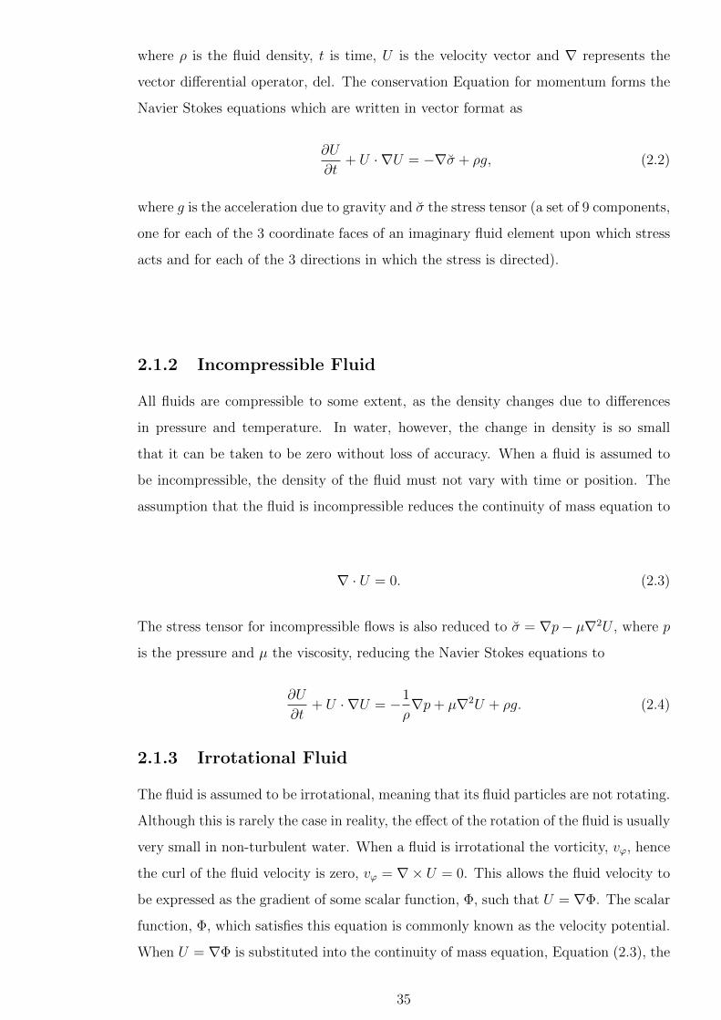
The flow past arrays of wave energy devices is assumed to be non-turbulent. Surface
turbulence is likely to occur during extreme storms, however the model does not need
to apply to this situation as in extreme storms survivability of the devices is prioritised
over energy extraction. The flow is assumed to be two-dimensional in the vertical
plane, with the horizontal and vertical coordinates, x and z respectively (see Figure
2.1).
2.1.1 Continuity Equations
A Newtonian fluid such as water must satisfy both a continuity Equation for mass and
a conservation Equation for momentum. A continuity Equation is a partial differential
Equation describing the transportation of a conserved quantity. The continuity Equa-
tion states that the rate at which mass enters a system is equal to the rate at which
mass leaves the same system. This is written mathematically as
∂ρ
∂t+∇ · (ρU) = 0, (2.1)
34
where ρ is the fluid density, t is time, U is the velocity vector and ∇ represents the
vector differential operator, del. The conservation Equation for momentum forms the
Navier Stokes equations which are written in vector format as
∂U
∂t+ U · ∇U = −∇σ + ρg, (2.2)
where g is the acceleration due to gravity and σ the stress tensor (a set of 9 components,
one for each of the 3 coordinate faces of an imaginary fluid element upon which stress
acts and for each of the 3 directions in which the stress is directed).
2.1.2 Incompressible Fluid
All fluids are compressible to some extent, as the density changes due to differences
in pressure and temperature. In water, however, the change in density is so small
that it can be taken to be zero without loss of accuracy. When a fluid is assumed to
be incompressible, the density of the fluid must not vary with time or position. The
assumption that the fluid is incompressible reduces the continuity of mass equation to
∇ · U = 0. (2.3)
The stress tensor for incompressible flows is also reduced to σ = ∇p− µ∇2U , where p
is the pressure and µ the viscosity, reducing the Navier Stokes equations to
∂U
∂t+ U · ∇U = −1
ρ∇p+ µ∇2U + ρg. (2.4)
2.1.3 Irrotational Fluid
The fluid is assumed to be irrotational, meaning that its fluid particles are not rotating.
Although this is rarely the case in reality, the effect of the rotation of the fluid is usually
very small in non-turbulent water. When a fluid is irrotational the vorticity, vϕ, hence
the curl of the fluid velocity is zero, vϕ = ∇× U = 0. This allows the fluid velocity to
be expressed as the gradient of some scalar function, Φ, such that U = ∇Φ. The scalar
function, Φ, which satisfies this equation is commonly known as the velocity potential.
When U = ∇Φ is substituted into the continuity of mass equation, Equation (2.3), the
35
resulting condition on Φ is known as Laplace’s Equation,
∇2Φ = 0. (2.5)
2.1.4 Inviscid Fluid
The fluid is further assumed to be inviscid, meaning it has zero viscosity (µ = 0).
Water has a low viscosity, so outside of boundary layers which are immediately adja-
cent to body surfaces its effects are negligible, justifying the inviscid approximation.
The inviscid assumption simplifies the Navier Stokes equations (Equation (2.4)) to the
following equation which is the vector form of Euler’s equations,
∂U
∂t+ U · ∇U = −1
ρ∇ (p+ ρgz) , (2.6)
where p is the pressure and −z the vertical distance below the free surface. In an
irrotational, incompressible and inviscid flow, the condition of irrotationality can be
used together with the velocity potential to reduce (2.6) to Bernoulli’s equation,
∂Φ
∂t+
1
2(∇Φ)2 − gz +
p
ρ= G(t), (2.7)
where G(t) is an arbitrary function of time only. By including the time dependence of
G in the velocity potential, G can be a constant instead of a function.
Laplace’s Equation can be solved subject to boundary conditions to find the velocity
potential on a body (partly or fully) submerged in a fluid with surface waves, which
can be used to determine the pressure distribution about the body using Bernoulli’s
equation, hence determine the forces on the body.
2.1.5 General Boundary Conditions
Resolution of forces on an immersed boundary requires solution of the flow problem
together with boundary conditions on the body boundary, the free surface and the
bottom boundary (see Figure 2.1) as well as a radiation condition.
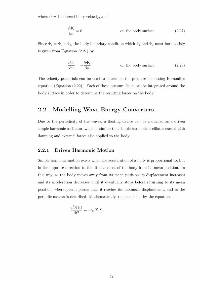
36
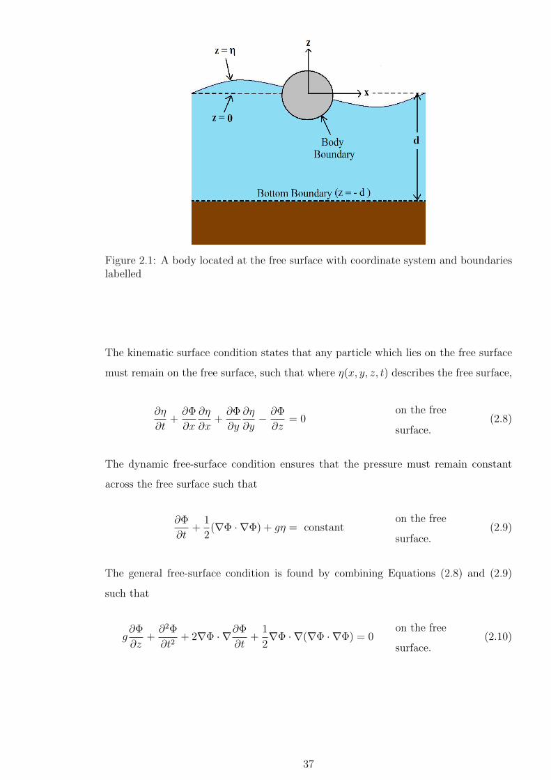
Figure 2.1: A body located at the free surface with coordinate system and boundarieslabelled
The kinematic surface condition states that any particle which lies on the free surface
must remain on the free surface, such that where η(x, y, z, t) describes the free surface,
∂η
∂t+∂Φ
∂x
∂η
∂x+∂Φ
∂y
∂η
∂y− ∂Φ
∂z= 0
on the free
surface.(2.8)
The dynamic free-surface condition ensures that the pressure must remain constant
across the free surface such that
∂Φ
∂t+
1
2(∇Φ · ∇Φ) + gη = constant
on the free
surface.(2.9)
The general free-surface condition is found by combining Equations (2.8) and (2.9)
such that
g∂Φ
∂z+∂2Φ
∂t2+ 2∇Φ · ∇∂Φ
∂t+
1
2∇Φ · ∇(∇Φ · ∇Φ) = 0
on the free
surface.(2.10)
37

Normal components of the velocity of the solid body boundary must be impressed upon
the fluid adjacent to it. The body surface boundary condition, where the body velocity
normal to the body surface is Ub, is therefore given by
∂Φ
∂n= Ub
on the body
boundary.(2.11)
Similarly, the bottom boundary condition is given by
∂Φ
∂z= 0 on z = −d. (2.12)
At infinity (horizontally) the radiation condition ensures that only outgoing radiated
waves exist. A formal, mathematical definition of the radiation condition is given in
Section 2.1.8 as it requires terminology which is not defined at this stage.
Once the total velocity potential is known, Bernoulli’s equation can be used to
determine the pressure throughout the fluid. The forces on the body can then be
found by integrating the pressure around the body. Determining the velocity potential
can however be complicated.
2.1.6 Linear Theory and Boundary Conditions
A common simplification of the boundary conditions is obtained from the Stokes ex-
pansion method which is achieved using the assumption that the wave amplitude and
hence wave height, H, are small compared to both the wavelength and the water depth.
The wave amplitude, Am, is the vertical distance from the undisturbed free surface to
the peak, which for a sinusoidal wave is half of the wave height such that Am = H2
. The
density of the wave crests, i.e. the number of wave crests per unit distance, is known
as the wavenumber, k, which relates to the wavelength such that k = 2πL
.
The velocity potential can be expanded into a perturbation series for the small
parameter, ε = kH2
as follows:
Φ = εΦ[1] + ε2Φ[2] + · · · (2.13)
On substituting Equation (2.13) into Laplace’s and Euler’s equations and the
boundary conditions, N th-order wave theory is formed by using only the terms of
order εN or below. 1st-order wave theory (in which all terms of order higher than ε are
neglected) is commonly called Linear Wave Theory, and higher order wave theory is
38
sometimes referred to as weakly non-linear wave theory to the N th-order. The effects
of including the second-order terms are considered in Chapter 4.
In linear wave theory, as the amplitude of the waves is small, the free-surface con-
dition is applied at z = 0 instead of z = η (see Figure 2.1). The linearised boundary
conditions are therefore given by:
Linearised Kinematic Surface Condition:
∂η
∂t− ∂Φ
∂z= 0 on z = 0; (2.14)
Linearised Dynamic Free-Surface Condition:
∂Φ
∂t+ gη = 0 on z = 0; (2.15)
General Free-Surface Condition
g∂Φ
∂z+∂2Φ
∂t2= 0 on z = 0, (2.16)
with
η = −1
g
(∂Φ
∂t
)
z=0
; (2.17)
Linearised Body-Surface Boundary Condition:
∂Φ
∂n= Ub on body surface; (2.18)
Linearised Bottom Boundary Condition:
∂Φ
∂z= 0 on z = −d. (2.19)
The radiation condition must also be satisfied ensuring only outgoing waves exist
at infinity. A formal, mathematical definition of the radiation condition is given in
Section 2.1.8.
Using the method of separation of variables to solve Laplace’s Equation subject to
39

the boundary conditions, the velocity potential can be determined to be
Φ(x, z, t) =gH
2ω
cosh (k(z + d))
cosh(kd)cos(kx− ωt). (2.20)
In the calculation of Φ, the assumption that the wave is periodic in x is used.
Equation (2.20) shows a linear relationship between the velocity potential and the
wave height. This ensures that the velocity potentials of component waves can be
summed together to determine the velocity potential of the resultant wave using the
theory of superposition. Although sinusoidal waves are very rare in reality, many other
more genuine waves shapes can be approximated by summing together a variety of
different sinusoidal waves in this manner.
The pressure field can be determined using the linear velocity potential in a lin-
earised form of Bernoulli’s equation in which the quadratic terms are ignored:
∂Φ
∂t− gz +
p
ρ= G. (2.21)
As the constant in Equation (2.7) is arbitrary it may be taken to be zero if required,
so that the linear pressure is given by
p =StaticPressure︷︸︸︷
ρgz −
DynamicPressure︷ ︸︸ ︷ρ∂Φ
∂t. (2.22)
2.1.7 Dispersion Relation
Substituting the derivatives of the velocity potential into the general free-surface con-
dition (Equation (2.16)) at the free surface (z = 0) provides an important relation
between the wave frequency, ω, and the wavenumber, k,
ω2 = gk tanh(kd). (2.23)
It is known as the linearised dispersion relation since, when written in terms of wave
celerity, the speed at which a wave crest travels, it shows that at a given depth, waves
with different wave numbers will travel at different speeds, a phenomenon known as
dispersion.
40
2.1.8 Incident, Scattered and Radiated Waves
The set of equations which the velocity potential must satisfy, that is Laplace’s Equa-
tion (Equation (2.5)), the boundary conditions (Equations (2.14) to (2.19)) and Bernoulli’s
equation (Equation (2.21)), is linear. This allows for the summation of component ve-
locity potentials to form the total velocity potential, hence allows for the division of
the wave problem into several sub-problems.
The wave body interaction problem is commonly divided into two sub-problems.
The first is the radiation problem where there are no incident waves but the body is
forced to oscillate with harmonic motion of specified frequency. The second is the exci-
tation problem (sometimes referred to as the diffraction problem in other texts) where
the body is subjected to a regular incident wave train whilst being restrained from
oscillating. The corresponding waves have velocity potentials Φr and Φr respectively.
The excitation velocity potential, Φe, can be split into two constituent parts, the
incident velocity potential, Φi, and the scattered velocity potential, Φs. The incident
velocity potential represents the incident waves, undisturbed by the body (as if the
body was not there). The excitation velocity potential represents the change in the
incident wave field due to the presence of the body.
The total velocity potential is therefore written as
Φ =
Φe︷ ︸︸ ︷Φi + Φs +Φr. (2.24)
The radiation condition applies only to the radiated waves, hence it is possible now
to formally define the radiation condition for the radial ordinate R (Sarpkaya and
Isaacson, 1981):
0 = limR→∞
[∂Φr
∂R− ikΦr
]. (2.25)
This condition at infinity ensures that the radiated waves must behave as outgoing
plane waves far from the body (Wehausen and Laitone, 1960).
In order for the total velocity potential, Φ, to satisfy the body boundary condition
given by Equation (2.18), the constituent velocity potentials must satisfy the following
body boundary conditions:
∂Φr
∂n= U on the body surface, (2.26)
41
where U = the forced body velocity, and
∂Φe
∂n= 0 on the body surface. (2.27)
Since Φe = Φi + Φs, the body boundary condition which Φi and Φs must both satisfy
is given from Equation (2.27) by
∂Φi
∂n= −∂Φs
∂non the body surface. (2.28)
The velocity potentials can be used to determine the pressure field using Bernoulli’s
equation (Equation (2.22)). Each of these pressure fields can be integrated around the
body surface in order to determine the resulting forces on the body.
2.2 Modelling Wave Energy Converters
Due to the periodicity of the waves, a floating device can be modelled as a driven
simple harmonic oscillator, which is similar to a simple harmonic oscillator except with
damping and external forces also applied to the body.
2.2.1 Driven Harmonic Motion
Simple harmonic motion exists when the acceleration of a body is proportional to, but
in the opposite direction to the displacement of the body from its mean position. In
this way, as the body moves away from its mean position its displacement increases
and its acceleration decreases until it eventually stops before returning to its mean
position, whereupon it passes until it reaches its maximum displacement, and so the
periodic motion is described. Mathematically, this is defined by the equation.
d2X(t)
dt2= −γ1X(t),
42
where X(t) is the displacement of the body (variation of position with time) and γ1
is a positive constant. For an undamped body undergoing simple harmonic motion,
the total force must satisfy Newton’s second law and Hooke’s law. Newton’s second
law states that the acceleration of a body is parallel and directly proportional to the
net force and inversely proportional to the mass. Hooke’s law states that for relatively
small deformations of an object, the displacement or size of the deformation is directly
proportional to the deforming force or load. Allowing the constant, γ1, to be of the
form γ1 = CM
where C is a constant and M the mass of the body, allows the force to
be written as
FTOT = Md2X(t)
dt2= −
Fres︷ ︸︸ ︷CX(t) . (2.29)
The right-hand side of Equation (2.29) represents a restoring force, Fres , with restoring
coefficient, C. For a simple harmonic oscillator, this is the only force acting on the
body. Adding a mechanical damping force, Fdamp, proportional to the velocity of the
body with damping coefficient, R, into this equation gives the equation of a damped
harmonic oscillator,
FTOT = Md2X(t)
dt2= −
Fdamp︷ ︸︸ ︷R
dX(t)
dt−
Fres︷ ︸︸ ︷CX(t) .
If an external driving force, Fext, is also present then the body becomes a driven
harmonic oscillator described by the equation
FTOT = Md2X(t)
dt2= Fext −
Fdamp︷ ︸︸ ︷R
dX(t)
dt−
Fres︷ ︸︸ ︷CX(t) .
This can be rearranged to give the equation
Fext = Md2X(t)
dt2+
Fdamp︷ ︸︸ ︷R
dX(t)
dt+
Fres︷ ︸︸ ︷CX(t) . (2.30)
2.2.2 Application to Wave Energy Devices
Wave energy devices are subject to external forces from the waves, namely the excita-
tion force, Fe, from the incident and scattered waves and the radiation force, Fr, from
the radiated waves, as well as a hydrostatic restoring force, Fres, and damping from
43
the power take-off system and friction, Fdamp. The forces are therefore described by
FTOT = Md2X(t)
dt2=
Fext︷ ︸︸ ︷Fe + Fr +Fdamp + Fres. (2.31)
If it is now assumed that the mechanical damping force varies linearly with velocity such
that FR = −RdX(t)dt
where R is the mechanical damping coefficient, and the hydrostatic
restoring force varies linearly with displacement such that Fres = −SX(t) for constant
S (known as the hydrostatic stiffness) then the wave energy device can be described
as a driven harmonic oscillator with equation
FTOT = Md2X(t)
dt2=
Fext︷ ︸︸ ︷Fe + Fr−
Fdamp︷ ︸︸ ︷R
dX(t)
dt−
Fres︷ ︸︸ ︷SX(t) .
Now, as the forces and motions are all periodic, the complex amplitudes can be con-
sidered (see Appendix B) to simplify the calculus so that
FTOT = MiωU =
Fext︷ ︸︸ ︷Fe + Fr−
Fdamp︷︸︸︷RU +
i
ω
Fres︷︸︸︷SU , (2.32)
where a hat symbol, ˆ , denotes the complex amplitude and U is the velocity of the
body.
2.2.3 Radiation Force and Velocity
The radiation force, Fr, can be split into the sum of two forces, the first is linear with
acceleration and the second is linear with body velocity. In this way the radiation force
can be written as
Fr = −(B
dX(t)
dt+ A
d2X(t)
dt2
), (2.33)
where B is known as the radiation damping and A the added mass. In terms of complex
amplitudes this can be written as
Fr = −(B + iωA) U , (2.34)
44

so Equation (2.32) can be rewritten as
FTOT = MiωU = Fe +
(−(B +R)− iωA+
i
ωS
)U . (2.35)
The body velocity can therefore be defined as
U =Fe(
(B +R) + iω(M + A− S
ω2
)) . (2.36)
2.3 Parameters
An unconstrained body is able to move in six possible directions, known as degrees of
freedom (see Figure 2.2). For an isolated device whose motion is restricted to i degrees
of freedom (where 1 ≤ i ≤ 6 as in Figure 2.2), the added mass (A), mechanical damping
(R), radiation damping (B) and hydrodynamic stiffness (S) are square matrices of
length i, and the excitation force (Fe) is a vector of length i.
Figure 2.2: Diagram of the three dimensional axes showing the 6 degrees of motion fora floating body
A single body that is only able to move in heave, which is the focus of this thesis,
will have single values for A, B, R, S, and Fe.
For an array of devices, the forces on each float will differ from those on an isolated
float due to scattering of the waves by all devices in the array. For an N element array
of bodies the square matrix and vector lengths (for A, R, B, S and Fe) are increased
to I × N . Where an array of N bodies are each restricted to motion in heave, the
focus of this thesis, the radiation damping component, Bi,j represents the radiation
45
damping on body i due to the radiation caused by an oscillation of body j with unit
amplitude. Similarly for components of the matrices (A, B and S). The excitation
force component (Fe)i represents the excitation force on body i.
2.4 Calculating Body Forces
The pressure due to the incident and scattered waves is determined using the exci-
tation velocity potential, determined by solving Laplace’s Equation together with the
boundary conditions, in Bernoulli’s equation. This pressure can be integrated around
the body to determine the excitation force, Fe. From herein, the excitation force will
be referred to as F to simplify the notation. Analytic solutions exist for the excitation
force for certain body geometries but, for arbitrary geometries, numerical solutions are
typically obtained using methods such as the boundary element method. Numerical
solutions can be readily obtained using computational analysis programmes such as
WAMIT. In this Section, the excitation force for a basic geometry is derived for a
range of wave frequencies and compared to the solution obtained using an approxima-
tion theory known as Froude-Krylov theory.
2.4.1 WAMIT
WAMIT is a program for computational analysis of the diffraction and radiation of
waves due to the interaction of surface waves with offshore structures. It can solve the
boundary value problem using either linear wave theory or second-order wave theory.
Both finite and infinite depths are permitted, as are fixed and floating bodies and
arrays of multiple bodies.
The boundary value problem is solved using an integral Equation method including
Greens functions together with a panel method. Further details of the theory used can
be found in Lee (1995). Geometries can be input into the program either as a series of
coordinates which form the vertices of panels which tessellate to form the surface, or
as analytically defined smooth, continuous surfaces known as patches.
WAMIT is able to compute many quantities such as the hydrostatic stiffness co-
efficients, added mass coefficients, radiation damping coefficients, excitation forces,
pressures and free surface elevation. All outputs from WAMIT are non-dimensional
complex amplitudes. Details on dimensionalising the output values are given in the
manual (WAMIT, Inc, 2008).
46

2.4.2 Froude-Krylov Theory
Froude Krylov theory can be used to approximate the excitation force on a small
body by multiplying the force due to the incident waves alone by a constant. When
a body is small compared to the wavelength, the velocity field on the body induced
by the incident waves can be assumed to be constant over the body such that Φs =
constant. Condition (2.28) becomes ∂Φe
∂n= ∂Φi
∂n= 0, suggesting that under these
circumstances, the excitation force can be approximated by the incident waves alone.
This small body approximation is known as the Froude-Krylov approximation, hence
the approximate excitation force is called the Froude-Krylov force, FFK , given by
integrating the pressure field around the body surface Sb due to the incident wave only.
The incident velocity potential is given by Equation (2.20), hence the dynamic pressure
due to the incident waves alone is determined using Bernoulli’s equation (Equation
(2.22)) as
pi = −ρgH2
cosh (k(z + d))
cosh(kd)sin(kx− ωt).
Integrating this around the body surface, Sb, gives the incident force
Fi =
∫∫
Sb
pi ndSb,
where n represents the normal to the body surface pointing into the fluid domain.
Therefore
Fi = − ρ g H
2 cosh(k d)
∫∫
Sb
( cosh(k(d+ z)) sin(k x− ω t)) ndSb. (2.37)
2.4.3 Application to a Hemispherical Float
The vertical (mode 3 in Diagram 2.2) force is now calculated for a hemispherical floating
body of radius a using the Froude-Krylov method and compared to the force obtained
using full Linear Theory through the application of the computer analysis program
WAMIT. The angle to the positive horizontal (x) axis is θ and the angle to the negative
vertical (z) axis is ψ (see Figure 2.3).
47

ax
z
d
Figure 2.3: Diagram to show coordinate system for hemispherical body of radius alocated at the free surface, in water of depth d
The x and z coordinates are given by
x = a sinψ cos θ (2.38)
and
z = −a cosψ (2.39)
respectively, the elemental area, dS, is given by
dSb = a2 sinψdθdψ (2.40)
and the the normals to the body surface pointing into the fluid domain in the x and z
directions are given by
nx = sinψ cos θ (2.41)
and
nz = cosψ (2.42)
48

respectively. The vertical component of the Froude-Krylov force on the hemispherical
body is therefore
FFKz =ρ g Ha2
2 cosh(k d)
∫ π/2
0
∫ 2π
0
cosh(k(d− a cosψ))
× cos(k a sinψ cos θ − ω t)
cosψ sinψdθdψ. (2.43)
These surface integrals can either be solved analytically or numerically. Both meth-
ods are shown here for comparison.
Analytic Solution of Froude-Krylov Forces on Hemispherical Float
The double integrals in Equation (2.43) can be solved analytically using the Bessel
function of the first kind and some well known identities (see Appendix D) to give
FFKz =πρ g Ha2
cosh(k d)(γ2 cosh (kd) + γ3 sinh (kd)) , (2.44)
where
γ2 =
1 + a2k2
8− a4k4
576+ a6k6
46080− a8k8
5160960+ a10k10
796262400− 29a12k12
78033715200
+ a14k14
249707888640− 53a16k16
337105649664000+ a18k18
6742112993280000− a20k20
148326485852160000
and
γ3 =
− 6758061133824000 ak+ 39070080 a11k11
− 868224 a13k13+ 19152 a15k15− 42 a17k17+ a19k19
· 1
10137091700736000.
Numerical Calculation of Froude-Krylov Forces on Hemispherical Float
Equation (2.43) can alternatively be evaluated numerically using the composite trape-
zoidal rule twice.
To do this, the angles θ and ψ must be divided into n Sections of size δθ and m
Sections of size δψ respectively such that
−→θ = [0, δθ, 2δθ, · · · , (θn−2)δθ, 2π]
and−→ψ = [0, δψ, 2δψ, · · · , (ψm−2)δψ,
π
2δψ].
49
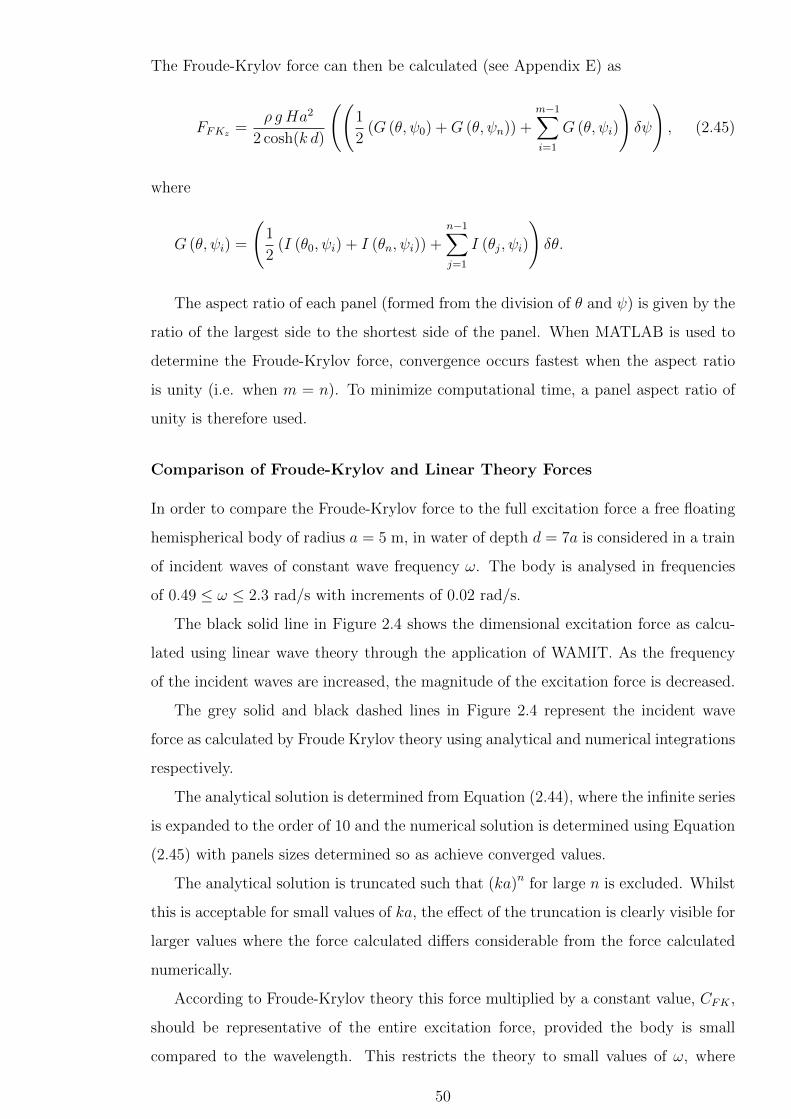
The Froude-Krylov force can then be calculated (see Appendix E) as
FFKz =ρ g Ha2
2 cosh(k d)
((1
2(G (θ, ψ0) +G (θ, ψn)) +
m−1∑
i=1
G (θ, ψi)
)δψ
), (2.45)
where
G (θ, ψi) =
(1
2(I (θ0, ψi) + I (θn, ψi)) +
n−1∑
j=1
I (θj, ψi)
)δθ.
The aspect ratio of each panel (formed from the division of θ and ψ) is given by the
ratio of the largest side to the shortest side of the panel. When MATLAB is used to
determine the Froude-Krylov force, convergence occurs fastest when the aspect ratio
is unity (i.e. when m = n). To minimize computational time, a panel aspect ratio of
unity is therefore used.
Comparison of Froude-Krylov and Linear Theory Forces
In order to compare the Froude-Krylov force to the full excitation force a free floating
hemispherical body of radius a = 5 m, in water of depth d = 7a is considered in a train
of incident waves of constant wave frequency ω. The body is analysed in frequencies
of 0.49 ≤ ω ≤ 2.3 rad/s with increments of 0.02 rad/s.
The black solid line in Figure 2.4 shows the dimensional excitation force as calcu-
lated using linear wave theory through the application of WAMIT. As the frequency
of the incident waves are increased, the magnitude of the excitation force is decreased.
The grey solid and black dashed lines in Figure 2.4 represent the incident wave
force as calculated by Froude Krylov theory using analytical and numerical integrations
respectively.
The analytical solution is determined from Equation (2.44), where the infinite series
is expanded to the order of 10 and the numerical solution is determined using Equation
(2.45) with panels sizes determined so as achieve converged values.
The analytical solution is truncated such that (ka)n for large n is excluded. Whilst
this is acceptable for small values of ka, the effect of the truncation is clearly visible for
larger values where the force calculated differs considerable from the force calculated
numerically.
According to Froude-Krylov theory this force multiplied by a constant value, CFK ,
should be representative of the entire excitation force, provided the body is small
compared to the wavelength. This restricts the theory to small values of ω, where
50
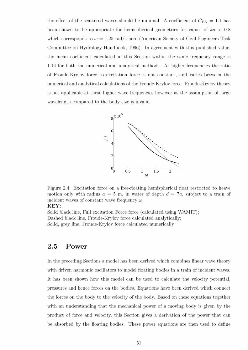
the effect of the scattered waves should be minimal. A coefficient of CFK = 1.1 has
been shown to be appropriate for hemispherical geometries for values of ka < 0.8
which corresponds to ω = 1.25 rad/s here (American Society of Civil Engineers Task
Committee on Hydrology Handbook, 1996). In agreement with this published value,
the mean coefficient calculated in this Section within the same frequency range is
1.14 for both the numerical and analytical methods. At higher frequencies the ratio
of Froude-Krylov force to excitation force is not constant, and varies between the
numerical and analytical calculations of the Froude-Krylov force. Froude-Krylov theory
is not applicable at these higher wave frequencies however as the assumption of large
wavelength compared to the body size is invalid.
0 0.5 1 1.5 20
2
4
6
8x 10
5
ω
Fe
Figure 2.4: Excitation force on a free-floating hemispherical float restricted to heavemotion only with radius a = 5 m, in water of depth d = 7a, subject to a train ofincident waves of constant wave frequency ωKEY:Solid black line, Full excitation Force force (calculated using WAMIT);Dashed black line, Froude-Krylov force calculated analytically;Solid, grey line, Froude-Krylov force calculated numerically
2.5 Power
In the preceding Sections a model has been derived which combines linear wave theory
with driven harmonic oscillators to model floating bodies in a train of incident waves.
It has been shown how this model can be used to calculate the velocity potential,
pressures and hence forces on the bodies. Equations have been derived which connect
the forces on the body to the velocity of the body. Based on these equations together
with an understanding that the mechanical power of a moving body is given by the
product of force and velocity, this Section gives a derivation of the power that can
be absorbed by the floating bodies. These power equations are then used to define
51

measures of the performance of individual devices within arrays.
2.5.1 Derivation of the Power Equations
The mechanical power, P , of a moving body is a function of the external force, Fext,
on the body multiplied by the body’s velocity, U , such that
P (t) = Fext(t)U(t). (2.46)
Using this relationship the time averaged power can be written in terms of the complex
amplitudes of Fext and U (see Appendix F) as
P =1
2<F ∗extU
, (2.47)
in which the superscript symbol, ‘∗’, represents the complex conjugate. The external
force comes from the waves and so is the sum of the excitation force, Fe, and radiation
force, Fr, (see Section 2.2.2), so its complex amplitude can be written (using Equation
(2.34)) as
Fext = F ∗e − U∗(B − iωA
). (2.48)
Substituting Equation 2.48 into Equation 2.47 results in the following equation for time
averaged power (see Appendix F for full derivation):
P =1
8F ∗eB
−1Fe −1
2
(U− 1
2B−1Fe
)∗B
(U− 1
2B−1Fe
). (2.49)
Using Equation (2.32), the external force from the waves could alternatively be written
as
Fext =
(−iω
(M +
S
ω2
)+R
)U . (2.50)
Substituting Equation 2.50 into Equation 2.47 results in an alternative Equation for
power,
P =1
2
(<UTRT<U+ =UTRT=U
), (2.51)
52

where the superscript symbol, ‘T ’ , represents the transpose of the matrices and < and
= represent the real and imaginary parts respectively. For an array of N devices A, B,
R, M and S are N ×N matrices, F is a vector of length N resulting in P representing
the net power, a single value for the whole array (see Section 2.3). Equation 2.51 can
be re-written in terms of the components of the U and R matrices such that
P =1
2
(N∑
i=1
N∑
j=1
<UiRTi,j<Uj+
N∑
i=1
N∑
j=1
=UiRTi,j=Uj
). (2.52)
In the specific case where R is a diagonal matrix transposing the matrix has no effect
such that RT = R and Ri 6=j = 0. This reduces Equation (2.52) to
P =N∑
i=1
PiRi,i for Pi =1
2Ri,i|Ui|2 (iff Ri 6=j = 0 ∀ 1 ≤ i, j ≤ N) . (2.53)
As the mechanical damping on an isolated device has only a single element, elements
with Ri 6=j do not exist, so Equation (2.53) is true also for an isolated device.
Whilst Equation (2.49), given in (Thomas and Evans, 1981), is the most general
Equation to calculate the net power, it does not indicate how much power is absorbed
by each individual device within an array. If the specific condition that the mechanical
damping matrix is diagonal is met, it is therefore beneficial to use Equation (2.53).
Equation (2.53) is also a more simple Equation to work with than (2.49), making it
the preferable Equation to calculate the power from an isolated device.
2.5.2 Optimal Power
Power output is maximum when the second term of Equation (2.49) vanishes (i.e.
when U = 12B−1F ). This is satisfied only when the force and velocity are in phase (i.e.
S = (M + A)ω2) and when the mechanical damping matrix R is identical to the dense
radiation damping matrix B (Thomas and Evans, 1981) so that
Pmax =1
8F ∗eB
−1Fe. (2.54)
53

2.6 Interaction Factors
2.6.1 Conventional Interaction Factor, q
The response of each float is dependent on both the excitation force due to the diffracted
wave-field and forcing due to waves radiated by the oscillation of the devices. It is
widely known that these interactions cause both the response and power output of a
float within an array to differ from the same device in isolation. A measure of the effect
of the hydrodynamic coupling between devices is commonly given by the interaction
factor q which is defined as:
q =Net power from array
N × Power from same device in isolation(2.55)
An interaction factor of q = 1 indicates that the devices within the array are producing
the same amount of overall power as if the same number of devices are in isolation,
whereas factors greater- or less-than one indicate constructive- or destructive interac-
tions. The interaction factor is therefore an important measure of the performance
of closely spaced arrays and it is particularly useful for developers to understand the
limiting values applicable to real systems.
54

0 0.5 1 1.5 2 2.50
1
2
3
ka
q
(a) s = 5a
0 0.5 1 1.5 2 2.50
1
2
3
ka
q
(b) s = 8a
(c) (Mavrakos and McIver, 1997) s = 5a
NB: dotted line represents alternative approx-
imation theory known as Plane Wave Theory
(discussed in Section 1.6.5) which is not calcu-
lated here
(d) (Mavrakos and McIver, 1997) s = 8a
NB: dotted line represents alternative approx-
imation theory known as Plane Wave Theory
(discussed in Section 1.6.5) which is not calcu-
lated here
Figure 2.5: Interaction factor, q, against ka where k is the wavenumber and a the floatradius for a 5× 1 array of circular cylinders with draft=radius, separation distance, s,in water of depth 8aKEY:Solid line, Calculated using full linear wave theory using WAMIT;Dashed line, Calculated using Point Absorber theory
Figure 2.5 shows the optimal interaction factor as calculated using Equation (2.55)
together with Equation (2.54) using the excitation force vectors and radiation damping
matrices as given by the wave analysis program, WAMIT. The data is shown for a 5×1
array of heaving vertical cylindrical floats of radius a and draught a in water of finite
depth, d = 8a for two separation distances, s = 5a and s = 8a, to allow for comparison
to the published Figure (Mavrakos and McIver, 1997, Figure 7). The similarity between
the published results of Mavrakos and McIver (1997) and those determined using the
WAMIT parameters is clearly visible.
55

(a) Black lines, Fixed k = 0.4a , varied s, directly
from (Thomas and Evans, 1981)
NB: dotted line represents alternative wave di-
rection (45o to the line of the array) which is
not considered in this thesis
0 2 4 6 8 100
1
2
3
ks
q
(b) Solid lines, varied k and fixed s = 4a (Thick
line, Beam seas and Thin line, head seas)
Figure 2.6: Interaction factor, q, for a 5 × 1 array of hemispherical floats in water ofinfinite depth where ks is varied by varying k, the wavenumber, compared to Figurea overlaid onto Figure 2 from Thomas and Evans (1981) and to an array where ks isvaried by varying s, the float separation distanceKEY:×, Beam seas as calculated using WAMIT results with fixed k = 0.4/a;o , Head seas as calculated using WAMIT results with fixed k = 0.4/a
Much of the research in this thesis is presented for hemispherical floats and so
the interaction factor for an optimally tuned (as described in Section 2.5.2) 5 × 1
array of heaving hemispherical floats of radius a is shown in Figure 2.6. Beam seas
represents the seas in which the train of incident waves propagates perpendicular to
the line of the array and head seas represents seas in which the train of incident waves
propagates along the line of the array. The markers show the optimal interaction factors
determined using WAMIT coefficients for an array in which ks is varied by changing
the separation distance, s, but keeping a fixed wave frequency and hence wavenumber,
k, such that ka = 0.4. It can be seen in Figure 2.6a that the resulting interaction
factors are the same as those published for the same array by (Thomas and Evans,
1981).
It could however be difficult to implement an array in which the separation distance
is varied according to the incident wave frequency. This thesis therefore focuses on
arrays in which the separation distance is fixed and the wave frequency is varied. The
solid lines in Figure 2.6b show the optimal interaction factors from such an array whose
spacing is fixed (s = 4a) in trains of incident waves of varying frequencies. The ratio of
device radius to wavelength varies over the range 0.2 < ka < 2.5 in this fixed spacing
56

array. The two cases are therefore only directly comparable for ks = 1.6. As the value
of ks decreases for the fixed spacing array, the amplitude of the wave-field scattered
by each device reduces.
The research presented in this report is predominantly in water of finite depth
whereas the data in Figure 2.6 is for an array in water of infinite depth. Using a finite
water depth presents a slight shift in the interaction factor curves shown in Figure 2.6
towards higher values of ks, although this is only significant at low ks values.
2.6.2 Normalised Interaction Factor, Q
The interaction factor, as given by Equation (2.55), is calculated relative to the power
of an isolated device, which is dependent on the damping applied to the isolated device
together with its mass. When comparing methods to vary the mass and mechanical
damping matrices for an array of devices, the interaction factor, or q-factor, although
widely used, can be misleading as the isolated devices to which the arrays are being
compared in the q-factor, are different. It can be more informative to compare the
power from an array of devices to the maximum power from the same number of
isolated devices with set mass and mechanical damping values:
Q =Net power from array
N ×
Maximum power from an isolated device
with a fixed mass and damping value
(2.56)
In this thesis Q uses a comparison to an isolated device having a mass of twice
its dry weight (M0 = 2Mm) and mechanical damping equal to the radiation damping
(R0 = B0). Figure (2.7) shows both types of interaction factor (q and Q) for two
five element arrays, one in which the float masses are each 1.5Mm, and one in which
they are 2Mm (where Mm is the displaced mass of fluid). Comparison of the q-factors
(Figure (2.7a)) shows that the performance within an array compared to in isolation is
better for the lighter floats than the heavier floats. This could however be misleading,
as this does not mean that the array of lighter floats is performing better than the
array of heavier floats, only that the interactions within the array are greater. As the
Q-factor instead gives the performance of both arrays relative to a fixed power value,
the comparison of the performance of both arrays relative to each other becomes much
clearer. It can be seen in Figure 2.7b that the heavier array (for which the individual
floats have a natural frequency of 1.07 rad/sec) is able to absorb significantly greater
power than the lighter array (for which the individual floats have a natural frequency
57
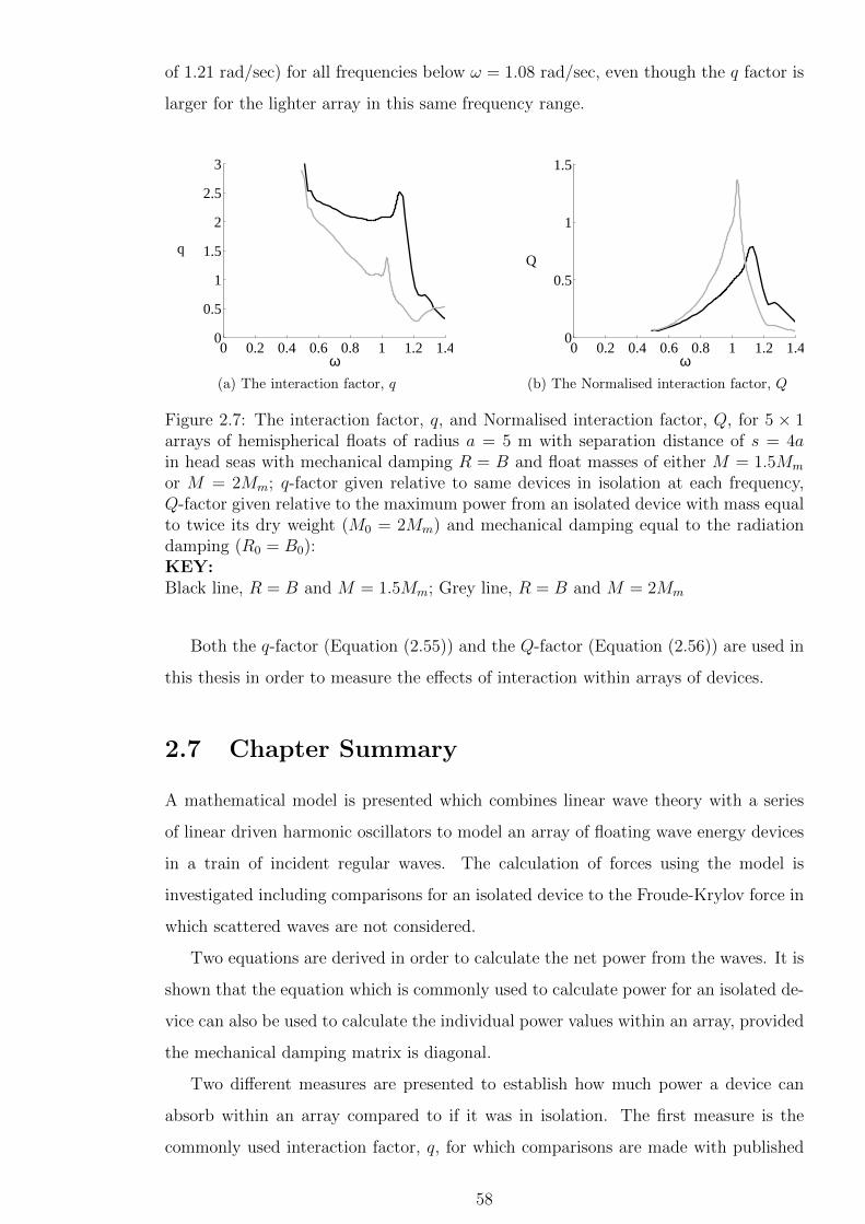
of 1.21 rad/sec) for all frequencies below ω = 1.08 rad/sec, even though the q factor is
larger for the lighter array in this same frequency range.
0 0.2 0.4 0.6 0.8 1 1.2 1.40
0.5
1
1.5
2
2.5
3
q
ω(a) The interaction factor, q
0 0.2 0.4 0.6 0.8 1 1.2 1.40
0.5
1
1.5
Q
ω(b) The Normalised interaction factor, Q
Figure 2.7: The interaction factor, q, and Normalised interaction factor, Q, for 5 × 1arrays of hemispherical floats of radius a = 5 m with separation distance of s = 4ain head seas with mechanical damping R = B and float masses of either M = 1.5Mm
or M = 2Mm; q-factor given relative to same devices in isolation at each frequency,Q-factor given relative to the maximum power from an isolated device with mass equalto twice its dry weight (M0 = 2Mm) and mechanical damping equal to the radiationdamping (R0 = B0):KEY:Black line, R = B and M = 1.5Mm; Grey line, R = B and M = 2Mm
Both the q-factor (Equation (2.55)) and the Q-factor (Equation (2.56)) are used in
this thesis in order to measure the effects of interaction within arrays of devices.
2.7 Chapter Summary
A mathematical model is presented which combines linear wave theory with a series
of linear driven harmonic oscillators to model an array of floating wave energy devices
in a train of incident regular waves. The calculation of forces using the model is
investigated including comparisons for an isolated device to the Froude-Krylov force in
which scattered waves are not considered.
Two equations are derived in order to calculate the net power from the waves. It is
shown that the equation which is commonly used to calculate power for an isolated de-
vice can also be used to calculate the individual power values within an array, provided
the mechanical damping matrix is diagonal.
Two different measures are presented to establish how much power a device can
absorb within an array compared to if it was in isolation. The first measure is the
commonly used interaction factor, q, for which comparisons are made with published
58

data. The second interaction measure, the Normalised Interaction Factor, Q, allows
for comparison between arrays of devices with different properties.
59
Chapter 3
Comparison to Experiment
Linear hydrodynamic analysis has been widely used to study the response of either
individual floating bodies or arrays of floating structures such as wave energy devices.
It has been shown that this approach is sufficient to determine the wave induced force on
fixed geometries and to predict the response of isolated floating geometries to regular
waves. However, there have been few studies which evaluate the accuracy of this
approach for predicting the response of the shallow draft floats that are generally of
interest for wave energy devices.
In this chapter the validity of linear theory is considered for predicting response
due to regular waves by comparing linear theory predictions of a line of five floats to
experimental measurements. The floats considered are shallow draft and arranged at
a separation distance of two diameters centre to centre.
3.1 Introduction
Experimental data for the forces on isolated devices of basic geometries have been
shown to be in close agreement with linear theory provided the wave amplitude re-
mains small compared to the body diameter (Evans et al. (1979b) and Chakrabarti
and Tam (1973)). Several experimental studies have been published of the response of
isolated floats that are based on designs for wave energy devices that are presently in
development (Count (1978), Greenhow et al. (1982), Vantorre et al. (2004) and Stal-
lard et al. (2009b)). Rigid structures which include small arrays of cylindrical bodies
such as Tension Leg or Gravity Based platforms and floating airports have prompted
experimental studies into the wave-structure interaction, finding large wave elevations
in the vicinity of the cylinders under certain wave conditions and array layouts (Swan
et al. (1997), Ohl et al. (2001) and Kagemoto et al. (2002)). However, there are few
60

published studies concerning experimental studies of arrays of floating wave energy
devices. Those that have been published have generally focused on comparison to ei-
ther predictions of optimal response (e.g. Budal et al. (1979)) or on specific device
configurations.
One of the earliest notable experimental studies of arrays of wave energy converters
was conducted by Budal et al. (1979) who reported measurements of the free-response
amplitude and power absorption of a (rigidly connected) pair of hemispherical ended
floats (radius a = 0.075 m , draft = a+0.1 m). The floats were located in a two-element
array across the width of a 1.01 m wide flume such that the centre of each float was
located 0.25 m from a side wall. This was intended to represent an infinitely long line
of tuned devices (with a natural frequency equal to the wave frequency) at s = 6.66a
spacing aligned with the wave crest. The measured power captured by the devices
confirmed predictions of point absorber theory in that the interaction factor (q-factor)
increases linearly toward π as the device spacing approaches the wavelength.
At a similar time, tests were conducted at the University of Edinburgh on behalf
of the UK Central Electricity Generating Board (Count, 1980). Interaction factors
were obtained for two linear arrays comprising two devices at non-dimensional spacing
ks = 7.48 and ten devices at ks = 4.99. Both cases show reasonable agreement
with point absorber predictions. Although some findings from this study have been
documented, detailed reports and measurements seem to be lost (Stallard et al., 2008).
In recent years, various device developers have conducted experiments to under-
stand the power output from prototype systems. This includes developers such as the
WaveStar which has had an array of 1:10 scale device in the sea from 2006 to 2010 and
a full scale array the sea since 2009 (Marquis, 2010) and the FO3 device array which
has been tested in the ocean with a single float and with an array of 4 floats at 13
scale
(de Rouck and Meirschaert, 2009). The variation of averaged power (excluding losses
in the power take-off) with significant wave height has been found to follow the same
trend at 13
scale in the sea as those determined for the 140
scale experimental wave tank
model. A large amount of scatter was, however, found to be present in the results
from the sea trials which is thought to be due to the variations in wave directions and
periods which were not accounted for in the experimental wave tank (Frigaard and
Lyke Anderson, 2008). Experimental data has been released for the AquaBuOY device
however these are based on a distinct and unusual power take off system involving a
large, vertical accelerator tube attached to the base of the float (Wacher and Neilsen,
2010).
61

The purpose of the present study is to compare predictions of the response of
a closely spaced array of floats obtained using linear analysis to experimental mea-
surements of a comparable system. Each float is the same geometry and mass and
mechanical damping is minimised such that the response amplitude is maximised. By
neglecting mechanical damping, which is usually applied via a power take-off system,
large response amplitudes tend to occur. The most onerous conditions for linear the-
ory, which is based on the assumption that motion amplitudes are small, are therefore
provided by neglecting mechanical damping.
The closely spaced array considered is comprised of heaving floats which are each
connected to a counterweight via a cable which is supported by a pulley system attached
to a fixed structure located above the waterline. This is a similar set-up to the device
analysed by Stallard et al. (2009b), except here multiple identical devices are arranged
in a closely spaced array and the float geometry is simplified to a uniform vertical
cylinder with a semi-ellipsoidal base. The level of mechanical damping applied to the
float can be specified using a dynamometer system which is an inherent part of the
experimental model. For the purpose of measurements reported in this study, friction in
the drivetrain is compensated for, thus float motion can be considered as mechanically
undamped. Further details regarding the dynamometer and its operation can be found
in Weller (2010).
3.2 Experimental Set-Up and Measured Response
The experimental equipment is described in Thomas et al. (2008) and details of the
experimental arrangement and procedures are given by Weller (2009). All experiments
were run as part of a PhD programme which was run in parallel to the research of
this thesis (Weller, 2010). Tests were conducted in a 5 m wide flume with a flat bed
of length 18.5 m from paddles to mid-beach. In all of the array tests, the middle float
was located at the centre-line of the flume (i.e. 2.5 m from both flume walls) and
3.6 m from the wave-paddles. Each float has a cylindrical section with an ellipsoidal
base with circular cross section of radius a1 = 0.076 m, draft radius (of the ellipsoidal
section) of a2 = 0.065 m and mass 1.2 kg.
The displaced mass of the float, Mm, was 0.8 kg with a supplementary mass, Msup,
of 0.8 kg, split into two sections; 0.4 kg added to the float, and 0.4 kg as a counter-
weight supported by a pulley in a similar manner to the approach used in (Vantorre
et al., 2004). In this way the total system mass was M = 2Mm without changing the
62

submerged geometry of the float. When in still water, the free surface was located at
the top of the ellipsoidal base. Experiments were conducted at 166
geometric scale of
the linear analysis conducted in WAMIT, for which the cross section radius was 5 m
and the draft radius was 4.28 m. Wave periods and system masses were obtained such
that Froude similarity was maintained. For the experimental set-up described in this
section, Froude-scaling was applied with a geometric scale factor of 66.
The float-counterweight pulley system was chosen over a strut support system to
minimise mechanical friction. Although this mechanism allowed each float to undergo
some motion in surge, horizontal motion observed was small relative to the incident
wavelength and so pulley rotation was a reasonable approximation to the vertical dis-
placement (Weller, 2010). Angular pulley displacements were measured using a digital
encoder on each device. Vertical float displacements were obtained by multiplying the
angular pulley displacements by the radius of the pulley, 0.0175 m. Six capacitance-
type wave gauges were used to record time varying wave amplitudes. For all tests,
the wave amplitude was specified as 0.013 m, equivalent to 0.86 m full-scale, and wave
frequencies in the range 0.75− 1.75 Hz were generated. The response amplitude ratios
reported were normalised relative to the measured wave amplitude.
For reference purposes, the floats are numbered from 1 to 5 as shown in Figure 3.1.
Figure 3.1: Diagram of 5× 1 array of hemispheres of radius a with a centre to centreseparation distance of s = 4a1; beam and head sea directions are also indicated
The experimentally measured response amplitude ratios are represented by markers
in Figures 3.2 and 3.4 for beam seas (where waves propagate perpendicular to line of
array) and in Figures 3.3 and 3.5 for head seas (where waves propagate along the line
of the array).
3.3 Numerical Prediction of Response
The response amplitude, |Xz|, of a body oscillating in heave due to an incident wave
of angular frequency ω can be obtained by integrating the float velocity as given by
63

Equation (2.36), such that
|Xz| =F
iω(R +B)− ω2(M + A− Sω2 )
. (3.1)
The study in this chapter concerns the response of mechanically unconstrained
devices as discussed in Section 3.1, such that mechanical damping, B, in Equation
(3.1) is zero. This assumes that mechanical friction is zero and hence power generation
is zero. Small amplitude motion is assumed and so hydrostatic stiffness S is typically
expressed in terms of water plane area, AWP , such that
S = ρg · AWP . (3.2)
It is straightforward to include linear mechanical damping in the model if required.
The response amplitude relative to the wave amplitude (12H) is known as the response
amplitude ratio, |dz|, and is given by
|dz| =2 |Xz|H
. (3.3)
Linear theory predictions with zero mechanical damping and stiffness calculated
using Equation (3.2) with the water plane area calculated when at rest (defined to be
stiffness calculation S1 in Section 3.3.1) are shown by the solid black lines in Figures 3.2
and 3.3. In general, agreement away from the peak of the predicted response appears
to be reasonable, although the measured response amplitude curve is shifted slightly
towards lower wave frequencies, with an apparent under-prediction of the response at
low frequencies. Near the peak frequency, the measured response is somewhat smaller
than predicted. Also, for beam seas, the predicted symmetry of response is not seen
in the experimental data (Float 2 different to 4).
3.3.1 Modified Stiffness & Damping
In this section two variations on the calculation of hydrostatic stiffness are considered
as well as a possible improvement in the agreement between the linear theory and
experimental results which could be achieved by including a small amount of additional
damping in the calculations. The four variations in the linear theory calculations are
represented by different lines in Figures 3.2 to 3.5.
64
Modified Hydrostatic Stiffness
For a device with a constant horizontal cross-sectional area such as a vertical cylinder,
the water-plane area is constant. A float with a non-uniform horizontal cross-sectional
area has a water-plane area which is dependent on draft. One of the fundamental
assumptions in linear wave theory is that the amplitudes of all oscillations are small.
In the initial calculation of hydrostatic stiffness, the variation of water-plane area due
to the heave motion of the float was therefore assumed to be negligible such that
S1 = ρg · AWP (X = 0) . (3.4)
When evaluated at the mean water line the radius is a1 but response amplitude ratios up
to 0.6a1 were observed during experiments. Over this range of displacement, the water
plane radius varies from 0.71a1 to a1 over this range. A more appropriate calculation
of stiffness should therefore account for this variation. The mean of the maximum and
minimum water-plane areas when the float oscillates with the mean response amplitude
measured experimentally (for all floats) is
S2 = ρg ·(
min(AWP
(X))
+ max(AWP
(X))
2
). (3.5)
X represents the mean of all of the time averaged response amplitudes measured ex-
perimentally such that
X =
∑Nω
i=1
∑Nj=1Xj (i)
Nω ·N, (3.6)
where Nω is the number of frequencies tested experimentally and N is the number
of floats. In beam seas, X = 1.61 m and in head seas X = 1.49 m. The response
amplitude ratios calculated using S2 are plotted on Figures 3.2 and 3.3.
Equation (3.5) is only intended to give an indication of the effect of hydrostatic
stiffness on response. It does not give an exact representation of the mean hydrostatic
stiffness on the floats as any phase differences between the wave and float responses
are neglected.
65
0
1
2
3
4
5Float 1
|dz|
Float 5
0
1
2
3
4
5Float 2
|dz|
0 0.2 0.4 0.6 0.8 1 1.2 1.4
Float 4
ω
0 0.2 0.4 0.6 0.8 1 1.2 1.40
1
2
3
4
5Float 3
ω
|dz|
Figure 3.2: Response amplitude ratio, |dz|, for each float within a 5 × 1 array ofhemispherical floats of radius a1 with centre to centre separation distance of s = 4a1
in BEAM seas.KEY: Markers, experimental data;Solid black line, Calculations with S = S1 (Equation (3.4)) and R = 0;Dotted black line, Calculations with S = S2 (Equation (3.5)) and R = 0
66

0
1
2
3
4
5Float 1
|dz|
Float 5
0
1
2
3
4
5Float 2
|dz|
0 0.2 0.4 0.6 0.8 1 1.2 1.4
Float 4
ω
0 0.2 0.4 0.6 0.8 1 1.2 1.40
1
2
3
4
5Float 3
ω
|dz|
Figure 3.3: Response amplitude ratio, |dz|, for each float within a 5 × 1 array ofhemispherical floats of radius a1 with centre to centre separation distance of s = 4a1
in HEAD seas.KEY: Markers, experimental data;Solid black line, Calculations with S = S1 (Equation (3.4)) and R = 0;Dotted black line, Calculations with S = S2 (Equation (3.5)) and R = 0
Additional Damping
As the experimental model does not include any power take-off systems applying a
damping force to the floats, the initial linear theory predictions were made using an
assumption of zero additional damping. The root mean square of the difference between
the numerical predictions and experimental data can however be reduced by including
a small amount of additional damping in the numerical model.
67
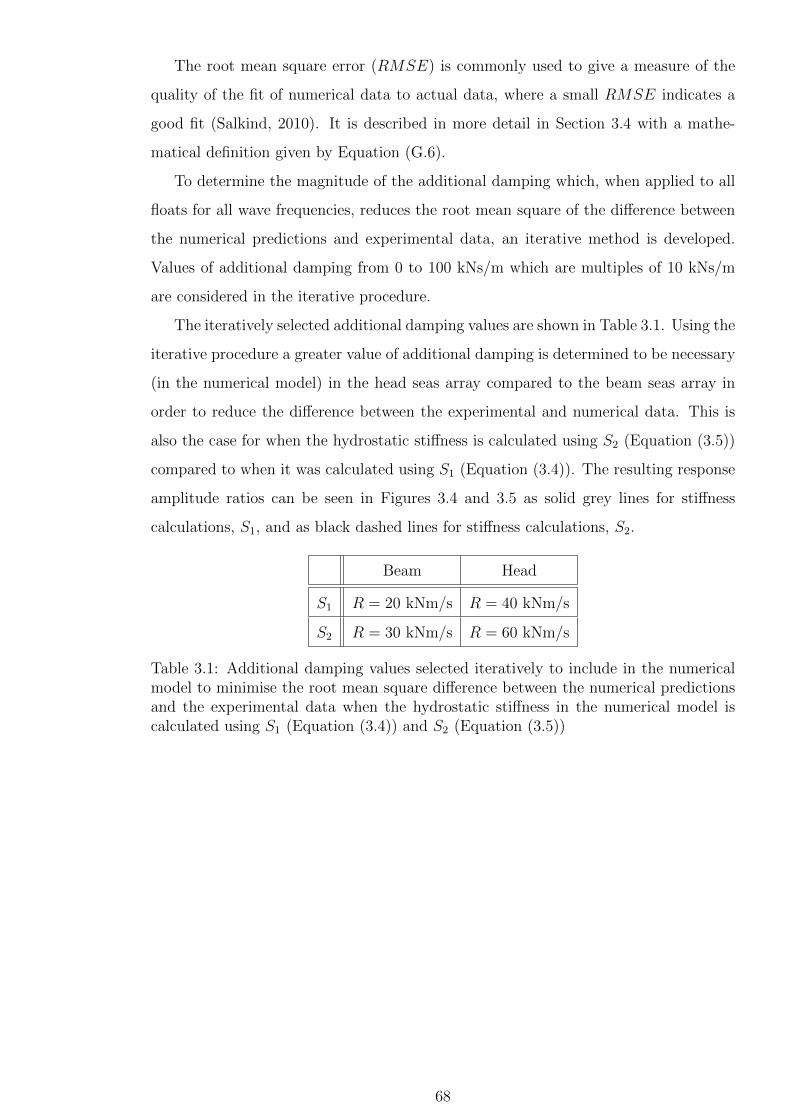
The root mean square error (RMSE) is commonly used to give a measure of the
quality of the fit of numerical data to actual data, where a small RMSE indicates a
good fit (Salkind, 2010). It is described in more detail in Section 3.4 with a mathe-
matical definition given by Equation (G.6).
To determine the magnitude of the additional damping which, when applied to all
floats for all wave frequencies, reduces the root mean square of the difference between
the numerical predictions and experimental data, an iterative method is developed.
Values of additional damping from 0 to 100 kNs/m which are multiples of 10 kNs/m
are considered in the iterative procedure.
The iteratively selected additional damping values are shown in Table 3.1. Using the
iterative procedure a greater value of additional damping is determined to be necessary
(in the numerical model) in the head seas array compared to the beam seas array in
order to reduce the difference between the experimental and numerical data. This is
also the case for when the hydrostatic stiffness is calculated using S2 (Equation (3.5))
compared to when it was calculated using S1 (Equation (3.4)). The resulting response
amplitude ratios can be seen in Figures 3.4 and 3.5 as solid grey lines for stiffness
calculations, S1, and as black dashed lines for stiffness calculations, S2.
Beam Head
S1 R = 20 kNm/s R = 40 kNm/s
S2 R = 30 kNm/s R = 60 kNm/s
Table 3.1: Additional damping values selected iteratively to include in the numericalmodel to minimise the root mean square difference between the numerical predictionsand the experimental data when the hydrostatic stiffness in the numerical model iscalculated using S1 (Equation (3.4)) and S2 (Equation (3.5))
68
0
1
2
3
4
5Float 1
|dz|
Float 5
0
1
2
3
4
5Float 2
|dz|
0 0.2 0.4 0.6 0.8 1 1.2 1.4
Float 4
ω
0 0.2 0.4 0.6 0.8 1 1.2 1.40
1
2
3
4
5Float 3
ω
|dz|
Figure 3.4: Response amplitude ratio, |dz|, for each float within a 5 × 1 array ofhemispherical floats of radius a1 with centre to centre separation distance of s = 4a1
in BEAM seas.KEY: Markers, experimental data (same as in Figure 3.2);Solid grey line, Calculations with S = S1 (Equation (3.4)) and R = 20 KNms−1;Dashed black line, Calculations with S = S2 (Equation (3.5)) and R = 30 KNms−1
69

0
1
2
3
4
5Float 1
|dz|
Float 5
0
1
2
3
4
5Float 2
|dz|
0 0.2 0.4 0.6 0.8 1 1.2 1.4
Float 4
ω
0 0.2 0.4 0.6 0.8 1 1.2 1.40
1
2
3
4
5Float 3
ω
|dz|
Figure 3.5: Response amplitude ratio, |dz|, for each float within a 5 × 1 array ofhemispherical floats of radius a1 with centre to centre separation distance of s = 4a1
in HEAD seas.KEY: Markers, experimental data (same as in Figure 3.3);Solid grey line, Calculations with S = S1 (Equation (3.4)) and R = 40 KNms−1;Dashed black line, Calculations with S = S2 (Equation (3.5)) and R = 60 KNms−1
3.4 Statistical Comparison of Methods
There are many different methods which can be used to validate a model by comparing
its predictions to the real world. A model can be shown to be invalid by its failure
according to a statistical test, however it cannot be shown to be valid as an inability
to show significant difference between the predictions of a numerical model and the
70

real world data may only be due to the power of the statistical test in that particular
application (Mayer and Butler, 1993). Any one statistical measure may be reliant on
rigid assumptions, so that if any one of the assumptions is not valid then the results
of the statistical test cannot be relied upon (Loague and Green, 1991). It is therefore
more thorough to consider a variety of different statistical measures together with a
subjective assessment of the data in a graphical format.
0 1 2 3 4 50
1
2
3
4
5
d[C]
d[E]
(a) S = S1 (Equation (3.4)) and R = 0
0 1 2 3 4 50
1
2
3
4
5
d[C]
d[E]
(b) S = S1 (Equation (3.4)) and R as given
by Table 3.1
0 1 2 3 4 50
1
2
3
4
5
d[C]
d[E]
(c) S = S2 (Equation (3.5)) and R = 0
0 1 2 3 4 50
1
2
3
4
5
d[C]
d[E]
(d) S = S2 (Equation (3.5)) and R as given
by Table 3.1
Figure 3.6: Response amplitude ratio, |dz|, for each float within a 5 × 1 array ofhemispherical floats of radius a1 with centre to centre separation distance of s = 4a1
in BEAM seas as measured experimentally (∣∣∣d[E]z
∣∣∣) and numerically (∣∣∣d[C]z
∣∣∣). The solid
lines mark the line |d[E]z | = |d[C]
z |. Numerical models use stiffness, S, and additionaldamping, R, as given in figure captionsKEY:Solid grey circular markers, ω ≤ 0.94 rad/s; Empty circular markers , ω > 0.94 rad/sFigures correspond to:(a) solid black lines in Figure 3.2; (b) solid grey lines in Figure 3.4; (c) dotted lines inFigure 3.2; (d) dashed lines in Figure 3.4
Mayer and Butler (1993) suggest that the accuracy of a model can be visualised
more easily when the actual data is plotted against the model data directly. Figures
71
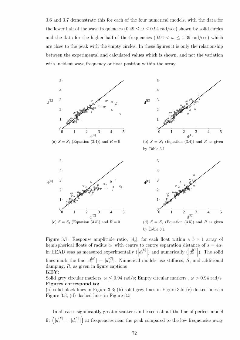
3.6 and 3.7 demonstrate this for each of the four numerical models, with the data for
the lower half of the wave frequencies (0.49 ≤ ω ≤ 0.94 rad/sec) shown by solid circles
and the data for the higher half of the frequencies (0.94 < ω ≤ 1.39 rad/sec) which
are close to the peak with the empty circles. In these figures it is only the relationship
between the experimental and calculated values which is shown, and not the variation
with incident wave frequency or float position within the array.
0 1 2 3 4 50
1
2
3
4
5
d[C]
d[E]
(a) S = S1 (Equation (3.4)) and R = 0
0 1 2 3 4 50
1
2
3
4
5
d[C]
d[E]
(b) S = S1 (Equation (3.4)) and R as given
by Table 3.1
0 1 2 3 4 50
1
2
3
4
5
d[C]
d[E]
(c) S = S2 (Equation (3.5)) and R = 0
0 1 2 3 4 50
1
2
3
4
5
d[C]
d[E]
(d) S = S2 (Equation (3.5)) and R as given
by Table 3.1
Figure 3.7: Response amplitude ratio, |dz|, for each float within a 5 × 1 array ofhemispherical floats of radius a1 with centre to centre separation distance of s = 4a1
in HEAD seas as measured experimentally (∣∣∣d[E]z
∣∣∣) and numerically (∣∣∣d[C]z
∣∣∣). The solid
lines mark the line |d[E]z | = |d[C]
z |. Numerical models use stiffness, S, and additionaldamping, R, as given in figure captionsKEY:Solid grey circular markers, ω ≤ 0.94 rad/s; Empty circular markers , ω > 0.94 rad/sFigures correspond to:(a) solid black lines in Figure 3.3; (b) solid grey lines in Figure 3.5; (c) dotted lines inFigure 3.3; (d) dashed lines in Figure 3.5
In all cases significantly greater scatter can be seen about the line of perfect model
fit(|d[E]z | = |d[C]
z |)
at frequencies near the peak compared to the low frequencies away
72

from the peak. The improved agreement when additional damping is included in the
numerical model (Figures 3.2 to 3.5), can be seen by the reduction in scatter of the
higher frequency data in Figures 3.6 and 3.7.
There are several statistical measures which can be used to determine which numer-
ical model provides the most similar results to the experimental data (see Appendix G
for mathematical definitions).
Variable Ideal S1 S2
Name Value R = 0 R as in Table 3.1 R = 0 R as in Table 3.1
MAE 0 0.24 0.24 0.34 0.21
MAPE 0 12.6 % 12.6 % 18.0 % 11.3 %
MAEPM 0 12.7% 12.9 % 18.2 % 11.3 %
RMSE 0 0.34 0.31 0.55 0.29
RMSPE 0 23.7 % 21.6 % 38.1 % 20.8 %
RMSEPM 0 18.2 % 16.6 % 29.1 % 15.5 %
CRM 0 0.03 0.09 -0.12 -0.01
PDV 0 - 0.41 0.14 -1.15 0.18
ME 0 1.32 1.12 2.38 0.90
CD 1 0.70 1.05 0.43 1.21
EF 1 0.60 0.66 -0.04 0.70
Table 3.2: Statistical measures of suitability of numerical models based on linear theoryfor application to experimental data for arrays in BEAM seas. Numerical models havehydrostatic stiffness calculated as S1 (Equation (3.4)) or S2 (Equation (3.5)), andadditional damping is either excluded (such that R = 0) or included with values asgiven in Table 3.1; Statistical definitions are given in Equations (G.5) to (G.15) inAppendix G; the best numerical model is indicated by bold font for each statisticalmeasure
Table 3.2 shows that of the four numerical models, the most appropriate in beam
seas is the use of linear theory with the hydrostatic stiffness calculated using S2 (Equa-
tion (3.5)) and additional damping included such that R = 30 kNm/s (as given by
Table 3.1). Nine out of the eleven statistical measures found this model favourable,
with the only exception being PDV and CD indicating that the linear theory model
with the inclusion of additional damping but stiffness calculated using S1 (Equation
(3.4)) provided a closer variance to the experimental data than the other three models.
Table 3.3 shows that in head seas the linear theory models including additional
damping are preferable over those which do not include any, with five statistical mea-
73

sures indicating that calculating the stiffness with S2 is preferable, and six indicating
that stiffness calculation S1 is preferable. The statistical measures for both models
including additional damping are similar in all eleven cases.
The selected models (in beam and head seas) predict data with means at most
5% different to the experimental data and variances at most 14% different from the
experimental data. A perfect fit would result in an EF value of 1, and a poor fit in an
EF value below zero, so EF values around 0.8 as given by the selected models indicate
a relatively good overall fit. A maximum response amplitude ratio error of around 0.9
is however determined in both head and beam seas by the selected models, which is
around 50% of the mean experimental value, showing that the numerical models are
good for giving an indication of the expected response amplitude ratio, but not the
exact value particularly close to the peak wave frequency.
Variable Ideal S1 S2
Name Value R = 0 R as in Table 3.1 R = 0 R as in Table 3.1
MAE 0 0.44 0.25 0.71 0.22
MAPE 0 24.6 % 15.9 % 34.4 % 13.7 %
MAEPM 0 25.0 % 14.3 % 41.0 % 12.5 %
RMSE 0 0.79 0.31 1.27 0.32
RMSPE 0 54.6 % 23.5 % 80.0 % 23.7 %
RMSEPM 0 45.2 % 17.6 % 72.7 % 18.1 %
CRM 0 -0.12 0.06 -0.30 0.05
DV R 0 -2.16 -0.05 -5.34 -0.10
ME 0 3.76 0.89 5.48 1.09
CD 1 0.31 0.92 0.14 0.89
EF 1 -0.48 0.78 -2.83 0.76
Table 3.3: Statistical measures of suitability of numerical models based on linear theoryfor application to experimental data for arrays in HEAD seas. Numerical models havehydrostatic stiffness calculated as S1 (Equation (3.4)) or S2 (Equation (3.5)), andadditional damping is either excluded (such that R = 0) or included with values asgiven in Table 3.1; Statistical definitions are given in Equations (G.5) to (G.15) inAppendix G; the best numerical model is indicated by bold font for each statisticalmeasure
74

3.5 Discussion of Model Discrepancies
The large over-prediction in peak response determined using linear theory with the
basic stiffness calculation and zero additional damping is expected to be due to a
combination of factors. In this section an estimate is obtained of the magnitude of
damping or stiffness variation due to experimental processes and due to the modelling
assumptions. The intention is to understand which of the assumptions has the greatest
influence on response.
3.5.1 Mechanical Friction
The first factor is friction within the additional components of the dynamometer sys-
tem. Although power was not extracted from the devices during the experiments, the
float-pulley-counterweight system was still connected to the power take-off system. Cal-
ibration of the experimental dynamometer outside of the flume determined a value of
current equivalent to the static friction in the rotating system, which was programmed
into the circuit board as an offset current. Small variations in static friction were found
to exist due to variations in various factors including temperature and device usage. To
account for these variations, a calibration process was adopted involving deceleration
tests of the drivetrain in order to compensate for friction in the system. These small
variations in static friction were typically around 2 mA which is equivalent to a power
loss of 0.0017W (Weller, 2010). With a Froude Scaling factor of 66, this corresponds
to a power loss of P = 0.0017× 663 = 3.97 kW.
Assuming harmonic motion , this power loss can be written as a function of float ve-
locity and damping using Equation (2.53). The time averaged power can be calculated
from Equation (2.53) at frequency ω (corresponding to period, T ) such that
P =1
2T
∫ T
0
RXzdt. (3.7)
So, assuming periodic motion
Xz = |Xz| cos (ωt) ,
75

hence the velocity is given by
Xz = ω |Xz| sin (ωt) .
Substituting this back into Equation (3.7) gives
P =R |Xz|
2T
∫ T
0
(2π
T
)sin (ωt) dt,
where the frequency ω has been replaced with 2πT
and the R is taken to be the time
averaged mechanical damping. This can be integrated to give
P =π2 |Xz|T 2
R,
which can be rearranged to give
R =T 2
π2 |Xz|P =
4
ω2 |Xz|P . (3.8)
Using Equation (3.8), the maximum unaccounted friction force at full scale due
to a power loss of P = 3.97 kW is calculated to be 4825.9 kNm/s. Although this is
relatively large, it is subject to uncertainties in scaling (see Section 3.5.5).
3.5.2 Viscous Drag
The second factor is viscous drag, Ffd, an alternative form of drag experienced by
the float. This is defined as Ffd = 12CdU
2ACsZ where Cd is the drag coefficient, U
the float velocity and ACsZ the cross-sectional area of the float in the vertical plane
perpendicular to the direction of wave propagation. As the area does not change
significantly, ACsZ ≈ π × 5 × 4.28 = 33.59m2 (since float radii are 5 and 4.28 m), the
maximum viscous drag must occur when the velocity is maximum. The velocity can be
determined as the multiple of the complex amplitude of the response and iω. As only
the absolute amplitude and not the complex amplitude of the response is known for
the experimental array, the multiplication with ω indicates an approximate velocity.
The maximum velocity is approximately 3.4 m/s in beam seas and 3.2 m/s in head
seas at full scale. A spherical body with a velocity of 3.4 m/s is expected to have a
drag coefficient of the order of 5 (Massey, 1975). The maximum viscous drag in beam
seas is therefore Ffd = 52× 3.42× π× 5× 4.2763 = 1.9413 kNm/s. This corresponds to
76

only 6.5 % of the required 30 kNm/s.
3.5.3 Flume Walls
All numerical calculations are based on hydrodynamic parameters calculated for 33m
water depth (equivalent to 0.45m depth at the geometric scale considered) for the open
sea case. It is recognised that the hydrodynamic parameters for a body in a narrow
channel may differ from those in the open sea.
The excitation force and pressure field on arrays of fixed vertical cylinders has
been found to be significantly different in a channel when compared to the open sea,
even when the channel width is large compared to the array dimensions (Butler and
Thomas, 1993). However for floating bodies, it is the variation of radiation force
due to the channel walls which is more likely to contribute to the observed difference
between theoretically predicted and measured maximum response amplitudes. It has
been shown that a body restricted to heave only which is located on the centre line of
a channel of width 2sc will have a different absorption length to that of the open sea
case except in specific spacing to wavelength ratios (Bjarte-Larsson et al., 2006). The
absorption length is defined to be the power absorbed by a body divided by the power
available per unit crest width.
Maximum power absorption (given by Equation (2.54)) is a function of excitation
force and radiation damping, so the difference in maximum absorption between the
open sea and channel cases corresponds to a variation in the relationship between the
excitation force and radiation damping. This could therefore indicate a difference in
the radiation damping from the open sea to the channel.
The magnitudes of such a variation in radiation damping have not been investi-
gated, particularly not for free-float response, however they are not expected to be the
main contributors to the requirement of the additional damping in the linear theory
predictions as the experimental channel width considered here is significantly greater
than the array dimensions, hence the time taken for waves to reflect from the channel
walls to the array in order for the radiated wave to be affected is quite large.
The power per unit length of wave crest is given by Pw = 18ρgH2Cg where Cg is
the group velocity. Assuming that waves radiate uniformly from a body placed at the
centre of the channel, circular waves are generated. Consider an arc of such a circular
wave subtending an infinitesimally small angle, δθ, at a distance rc from the body such
that its length is δθrc. The power in this wave arc is constant and independent of its
distance from the body and given by Pc = Pw × δθrc = 18ρgH2Cgδθrc. As ρ, g, π and
77
Cg are also independent of rc, the wave height must be inversely proportional to the
square-root of the distance from the body such that H ∝ 1√rc
. If the body is placed at
the centre of a flume of width 2s, then the wave must travel a distance, s − a1 from
the body surface to the channel wall. If the initial wave height is H1, then at the flume
wall the wave height is given by H2 = 1√sH1. Assuming the wave is perfectly reflected
at the channel wall, then the reflected wave must travel a distance of s back to the
centre of the float (the point at which the radiation damping force is measured), at
which its wave height is
H3 =1√
2s− a1
H1. (3.9)
In the experiments discussed in this section the flume was 5 m in width such that
s = 2.5 m, and the body has a horizontal radius of a1 = 0.076 m, so
H3 = 0.45H1. (3.10)
The total radiation force is formed from the sum of the radiation force due to
the radiation of a wave of unit amplitude and the force due to the reflected wave of
amplitude 45 % of the originally radiated wave. After travelling a distance of (2s− a1),
the reflected wave has a phase difference of ϑ = (2s−a1)L× 2π compared to the original
radiated wave.
The radiation force can be written using Equation (2.33) as
− Fr = BU + AU, (3.11)
where B is the radiation damping, A the added mass, U the float velocity and U the
float acceleration. This ordinarily represents the radiation force due to an oscillation
of unit amplitude. According to Equation (3.10), when the reflection of the radiated
wave reaches the origin, its wave height is 45 % of the original wave height. If there is
zero phase difference between the originally radiated wave and the reflected radiated
wave at the centre of the origin, the radiation damping and added mass coefficients are
therefore 45% of those originally calculated. These must therefore be summed together
with the originally calculated coefficients to give the actual added mass and radiation
damping coefficients.
The wavelength of the radiated wave varies according to the incident wave frequency
78
however, whilst the distance the wave must travel before returning to the origin is fixed.
A phase shift (ϑ) between the original and radiated waves will therefore be experienced
at most frequencies. The added mass and radiation damping are known before the
phase shift is implemented. Before the phase shift of ϑ, the velocity can be written as
U = |U | cos (ωt− ϑ) and the acceleration as U = −ω |U | sin (ωt− ϑ). The radiation
force can thus be rewritten as
−Fr = B |U | cos (ωt− ϑ) + A |U | (−ω sin (ωt− ϑ)) . (3.12)
Using trigonometric identities this can be rearranged such that the force is written in
the form of Equation (3.11) in terms of the velocity, U = |U | cos (ωt), and acceleration,
U = −ω |U | sin (ωt), after the phase shift of ϑ. The radiation damping and added mass
which would be experienced after the phase shift can therefore be written as
Bϑ = cos (ϑ)B + ω sin (ϑ)A (3.13)
and Aϑ = − 1
ωsin (ϑ)B + cos (ϑ)A (3.14)
respectively. The magnitude of the phase shift between the originally radiated wave
and the reflected wave therefore determines the magnitude of the variation in added
mass and radiation damping.
In head seas (at full scale), float 1 achieved the greatest Response Amplitude Ratio
at ω = 1.09 rad/sec (corresponding to a wavelength of L = 51.79 m). This corresponds
to a small-scale wavelength of L = 0.79 m which corresponds to a phase shift of
ϑ = 6.25 × 2π = 12.5 × π = 0.5π. Applying this to Equation (3.13) results in a
variation in radiation damping of B0.5π = 0. At this wave frequency the calculated
radiation damping is therefore not affected by the reflected wave (although the added
mass is affected).
The phase difference is however highly dependent on the precise frequency. Consider
for example the frequency of ω = 1.09 rad/sec at full scale (only one increment lower
than the peak Response Amplitude Ratio frequency of 1.09 rad/sec). This corresponds
to a small-scale wavelength of 6.49 (2s− a1) hence a phase shift of ϑ = 6.0287× 2π =
12.0574π. At this wave frequency the sum of the first row of the calculated radiation
damping matrix is 122.99 kNs/m and the sum of the first row of the calculated added
mass matrix is 113970 kg. The radiation damping due to the reflected wave is therefore
B0.9838π = cos(12.0574× π)× 0.45× 122990 + sin(12.0574× π)× 0.45× 113970 = 63.6
79
kNs/m. Similarly at ω = 1.11 rad/sec (full scale) the radiation damping due to the
reflected wave is -48 kNs/m.
These calculations indicate that the variation in radiation damping within the ex-
periments due to reflected waves could account for the majority of the discrepancy
between the numerical and experimental data at certain wave frequencies. The calcu-
lations are only indicative however and the magnitude by which the radiation damping
is modified within the experiments is highly sensitive to the wave frequency.
3.5.4 Variations in Spacing
Variations in spacing along the array due to oscillations in surge were visible during the
experiments, particularly in head seas. The large peak in the linear model is sensitive
to the phase of the excitation force and so may be inhibited by small variations in
float spacing caused by oscillations in surge. At rest the devices had a centre to
centre spacing of s = 4a which is the spacing used in the numerical calculations. The
movement of floats noticed during the experiments was less than a float radius. That
is, the instantaneous spacing between floats when oscillating in surge reduced by about
1 radius. This could correspond to a change of mean spacing, δs << a.
A phase shift caused by the variation in spacing would result in a greater radiation
damping due to the inclusion of parts of both the undisturbed radiation damping and
added mass according to Equation (3.13). The phase shift is given by ϑ = 2π δsL
where
δs is the change in spacing and L the wavelength.
In head seas (at full scale), the greatest Response Amplitude Ratio at ω = 1.09
rad/sec (L = 51.79 m) occurred on float one. At this frequency, the sum of the first
row of the radiation damping matrix is given by B (x− δx) = 118.56 kNs/m and the
sum of the first row of the radiation damping matrix is given by A (x− δx) = 110910
kg. A shift in mean body position of δx = 0.5a would result in a phase shift ϑ (0.5a) =
0.61. The radiation damping therefore becomes B(x) = 166.33 kNs/m, an increase of
47.8 kNs/m compared to the calculated radiation damping. This increase in radiation
damping due to the change in spacing is greater than the additional damping that
was required in head seas when the basic hydrostatic stiffness calculation was used
(R = 40kN/s).
80

3.5.5 Scaling Approximations
Each of the five experimental floats were hand-made to the same specifications, however
discrepancies of up to 0.5 mm are inherent in the float major and minor axis.The
proportions of the body were assumed to remain unchanged when scaled, however if
the dimensions of the experimental floats were larger than intended in one direction and
smaller than intended in another then this could result in the proportions of the bodies
being changed, causing the added mass and radiation damping of the experimental
body to differ from those of the numerical calculations. If the discrepancies occurred
in the float dimensions such that their proportions remained intact then the Froude
scaling factor would be in the range 65.4 < SF ≤ 66.2, causing the full scale mass
to be 0.66 % greater or smaller than that used in the calculations (in which a scaling
factor of SF = 65.8 was used). The calculation of the hydrostatic stiffness was based
on the full scale water-plane area which was 5 m irrespective of any discrepencies in
the experimental float measurements so would not experience a variation due to the
errors. The variation in the mass due to the scaling factor discrepancy means that the
natural frequency of an isolated float could have been over- or underestimated by 0.02
rad/s, which is half of the difference between the natural frequencies calculated with
the two different stiffness calculations, S1 and S2.
3.6 Chapter Conclusion
Predictions of free float response for a 5× 1 array of free-floating hemispherical floats
made using linear wave theory are compared to experimental data scaled up to full-
scale from a 166
scale test array. Power take-off is not considered so that large response
amplitude ratios occur. This provides a more stringent test for linear wave theory than
an array in which float motion is subject to mechanical damping.
Four possible cases are considered using linear wave theory such that the stiffness
is either calculated by assuming negligible change in water-plane area or by accounting
for the vertically non-uniform geometry by using a mean water-plane area, as well
as either including or excluding additional damping. In the cases where additional
damping is applied, the same amount is applied on all floats at all wave frequencies
with its value selected iteratively so as to minimise the root mean square error of the
numerical calculations to the experimental data.
A range of statistical measures are calculated to assess the fit of each of the four nu-
merical models to the experimental measurements. As a general rule (in both beam and
81

head seas) calculations made using linear theory in which a small amount of additional
damping is included and the stiffness is calculated using the mean water-plane area
(so as to account for the non-uniform cross-sectional area of the floats) are determined
to be in closest agreement with the experimental data. In head seas however, linear
theory calculations including additional damping and hydrostatic stiffness calculated
assuming negligible change in water-plane area are also found to be in close agreement
with the experimental data.
The experimental response amplitude ratios are found to be consistently close to 1.5
at low frequencies but form a peak at high frequencies with response amplitude ratios
of up to 3.52. The selected numerical models provide response amplitude ratios with
the same general trend as the experimental data. The selected numerical models have
a Root Mean Square Error in response amplitude ratio of around 0.3 and Modelling
Efficiency values (for which one indicates a perfect fit and zero a poor fit) of between
0.7 and 0.78 indicated a good overall agreement with the experimental data. The
agreement between the experimental and numerical data is found to be consistently
good at frequencies far from the peak, with the largest discrepancies found close to the
peak frequency.
The improved fit between the experimental data and linear model simulations in
which a small amount of additional damping was included, can be explained by phe-
nomena observed in the small-scale experiments which were not accounted for in the
numerical model. These phenomena include influence of mechanical friction and small
differences between the actual and modelled float geometries which become significant
when Froude scaling is applied. In addition, it is shown that the linear radiation damp-
ing force used in numerical predictions may differ from the actual radiation damping.
These discrepancies may occur due to the presence of flume walls and due to small
changes of the mean spacing between individual floats. The latter is particularly im-
portant for the head seas array in which change of spacing was observed during the
experiments.
82
Chapter 4
Second Order Forcing
It was explained in Chapter 2 that the total velocity potential, Φ, can be expressed as
a perturbation series of the wave-slope parameter, ε = kH2
, where k is the wavenumber
and H is the wave height, such that
Φ = εΦ[1] + ε2Φ[2] + ε3Φ[3] + · · · (4.1)
The first-order problem, used in the numerical models of Chapter 3, is only able to
account for loads and forces at frequencies within the incident wave spectrum. When
second-order terms are considered, the velocity potential also includes components
at the sums- and differences of pairs of component frequencies of the incident wave
spectrum. These sum and difference frequencies are often not part of the incident wave
spectrum. Second-order effects are therefore greatest at small and large frequencies
relative to the peak frequency of the spectrum (corresponding to difference and sum
frequencies respectively). This can become important if the sum or difference frequency
coincides with the natural frequency of a body, or if the damping or restoring forces at
that frequency are small (Kim and Yue, 1989).
The natural frequency of a heaving float, ω0, is a function of hydrostatic stiffness,
S, (proportional to the water-plane area), the added mass, A, and the system mass,
M , such that ω0 =√
SA+M
. Wave energy devices commonly have a natural frequency
which is higher than the peak frequency of the most common sea-states at the planned
deployment site. This allows for smaller devices (with smaller water-plane areas hence
smaller hydrostatic stiffness) and provides suitable circumstances for control systems
such as latching to be implemented where necessary (Babarit et al. (2004) and Falcao
(2008)). Since the natural frequencies of wave energy devices are typically high, it is
possible that second-order effects at sum frequencies could be significant close to the
83
natural frequency of the devices. Since wave spectra may be broad banded, second-
order effects at difference frequencies may also be important at the frequency which
corresponds to double the natural period of the device (i.e. ω0/2), particularly for high
wave periods.
The aim of this chapter is to gain an understanding of the magnitude of first- and
second-order forces on a small, closely spaced, array of wave energy devices. Different
sea-states (defined in Section 4.3) are considered with a view to determining a rela-
tionship between the frequencies at which second-order effects are important within a
closely spaced array and the significant wave height and peak period of the incident
wave spectrum.
A short review of the published research to date on second-order effects is given in
Section 4.2 with a discussion on how this relates to second-order effects in arrays of
wave energy devices. Section 4.4 describes the method used in this chapter to compare
the first- and second-order forces using wave amplitudes calculated from wave spectra
to dimensionalise the force given by the computer analysis program, WAMIT. As the
calculation of non-dimensional second-order forces using WAMIT is computationally
demanding, a coarse frequency increment is initially used to obtain the non-dimensional
forces. Section 4.5 provides a study to show the convergence of the dimensional forces
using decreasing frequency increments of interpolated non-dimensional forces. The
ratio of second to first-order forces is then analysed in detail in Section 4.6 using the
interpolated data for the different sea-states.
4.1 Second Order Solution Methods
To obtain second-order contributions to the velocity potential, a boundary value prob-
lem is typically solved. This is more complicated than the first-order boundary value
problem (Section 2.1.6) since the free-surface boundary condition is inhomogenous.
The inhomogeneous part of the condition consists of quadratic products of the first-
order potential together with a term containing the second-order potential. There are
two main approaches for solving the second-order problem, a direct approach and an
indirect approach.
The indirect approach avoids the direct calculation of the second-order potential
by defining an additional radiation potential. In this way, the second-order forces
and the distribution of wave pressures on a body can be determined (Eatock Taylor
et al., 1989). This approach does not require calculation of the complete second-
84
order velocity potential and so does not calculate the free-surface elevation at field
points or the wave run-up on a structure (Mavrakos and Chatjigeorgiou, 2009a). Even
though this method avoids the direct calculation of the second-order potential, the
numerical effort is not reduced significantly (Newman, 2001). Published research on
the indirect method include Lighthill (1979), Molin (1979), Eatock Taylor and Hung
(1987), Masuda et al. (1986), Masuda et al. (1987), Abuk-Azm and Williams (1988a),
Abuk-Azm and Williams (1988b), Abuk-Azm and Williams (1989a) and Abuk-Azm
and Williams (1989b).
The direct approach to solving the second-order boundary value problem requires
the direct integration of the pressure over the body surface. This is more computation-
ally complex than the indirect method but results in the calculation of the second-order
diffraction potential and so allows for the calculation of local flow features away from
the body such as the pressure field or the free-surface elevation. The second-order free-
surface elevation consists of a part due only to the second-order velocity potential and
two parts which are due only to the first-order velocity potential. The parts which are
due to the first-order potential consist of quadratic functions of the first-order velocity
potential. Published research on the direct method include Kim and Yue (1989), Chau
and Eatock Taylor (1988), Kriebel (1990), Chau and Eatock Taylor (1992), Newman
(1990b), Huang (1996a), Eatock Taylor and Huang (1997a), Eatock Taylor and Huang
(1997b), Malenica et al. (1999), Mavrakos and Chatjigeorgiou (2006) and Mavrakos
and Chatjigeorgiou (2009b).
An approximation theory based on the direct approach with the assumption of large
depth has been developed which does not attempt to satisfy the radiation condition or
the boundary condition on the body surface. It has been found to give similar results for
the second-order vertical force acting on a truncated surface piercing circular cylinder
at low frequencies to those obtained numerically using the complete direct method with
finite depth, but exceeds the numerical computations by 10-20 % at high frequencies
(Newman, 1990a).
A semi-analytical method of solution for the second-order diffraction problem in
which integrals are analysed both numerically in a finite domain containing the body
(or bodies), and analytically in an outer region extending to infinity in the horizontal
plane is commonly used in both the application of the indirect method (Ghalayini and
Williams, 1991) and direct method (Kim and Yue, 1989).
In this chapter the direct approach is applied via the wave analysis program,
WAMIT, however an option to use the indirect approach does also exist in WAMIT.
85
Within WAMIT, the free surface integral is evaluated numerically in the inner inte-
gral domain, and analytically in the (evanescent-wave free) outer domain by means
of expanding the Green function and the asymptotes of the first-order potentials in
Fourier-Bessel series (see the WAMIT theory manual for further details (Lee, 1995)).
4.2 Second Order Effects
Both the indirect and direct methods have received much attention since the 1970s,
however much of the published research is focused on the development of methods as
opposed to the results of the application of the methods. Most of the results concerning
the application of the second-order models to bodies have focused on the application to
isolated bodies, however limited research on second-order effects in multi-body prob-
lems does exist. Second-order effects including wave run-up, pressure and forcing on
moving bodies has received extremely limited research. The following sections give a
brief overview of the results which have been published to date concerning second-order
effects on both isolated bodies and arrays of fixed and oscillating bodies.
4.2.1 Fixed Isolated Bodies
The approximation theory based on the direct approach with the assumption of large
depth has been used to show that the second-order pressure is inversely proportional
to depth. At large depths, second-order contribution to pressure is larger than the
first-order component (Newman, 1990a). This implies that the second-order potential
decreases more slowly with depth than the first-order potential.
The second-order body forces, pressure distributions and wave amplitudes have
been calculated for a bottom mounted uniform vertical cylinder and a truncated but
motionless conical island using an explicitly obtained second-order velocity potential
Kim and Yue (1989). The second-order effects are amplified in the case of the bottom-
mounted cone, and are greater than the first-order effects at certain phase differences
for steep incident waves.
Using a semi-analytical direct method, the second-order free-surface elevation around
a bottom mounted cylinder has been shown to be significantly different to that pre-
dicted by linear wave theory (Eatock Taylor and Huang, 1997a), and the first- and
second-order free-surface elevation for a fixed truncated cylinder has been shown to be
very similar to that of a bottom mounted cylinder (Huang, 1996a). The location of the
maximum free-surface elevation has also been shown to be dependent on the order to
86
which it is calculated (Huang, 1996a).
In the case of a bottom mounted circular cylinder, a direct semi-analytical method
has been used to show that a significant increase in wave run-up can occur if the
maximum second-order and first-order wave components are in phase (Eatock Taylor
and Huang, 1997b). Using a fully analytical direct method, the inclusion of second-
order effects on a bottom mounted circular cylinder has been shown to increase the
maximum wave crest run up by 50 % and the forces by 10 - 20 % compared to linear
theory (Kriebel, 1990).
Arrays of Fixed Bodies
The indirect (semi-analytical) method has been applied to arrays of bottom-mounted
vertical cylinders with cylindrical and elliptical cross-section, at two different spacings
(Ghalayini and Williams, 1991), finding that for spacings of 5a and 3a (where a is the
radius of the floats) the increase in the magnitude of the force due to second-order
effects is between 20 and 30 %.
Bottom -mounted cylinder arrays have also been analysed using a semi analytical
direct approach to determine second-order wave elevation and forces (Malenica et al.,
1999). The second-order surge force and pitch moment are considered on a 2×1 array, a
triangular array and a 2×2 array of cylinders separated by s = 6a in water of depth 3a.
Even though the second-order forces on individual cylinders within the array are larger
than those of an isolated cylinder for almost all of the frequency range considered, it
has been shown that the total array averaged second-order force is sometimes not large
due to phase differences between the cylinders.
Arrays of four cylinders in a 2 × 2 layout with separation distances of s = 4a and
s = 3.333a have also been considered by the same authors (Malenica et al., 1999).
At the frequencies at which linear near-trapping (see Section 1.6.4) has been shown
to occur, both the first-order elevations and the individual components of the second-
order elevation are large, but due to the phase differences between the second-order
components, the total second-order elevation is small. When the incident wave fre-
quency is half of the linear near-trapping frequency however, the wave elevation at
first-order, and at second-order due to the quadratic components of the first-order po-
tential only (see Section 4.1) were found to be unremarkable, whereas the component of
the second-order wave elevation due to the second-order potential was large, hence the
total second-order elevation was large. This suggests that second-order near-trapping
occurs when the double frequency associated with the second-order incoming wave co-
87
incides with the linear near-trapping frequency (Malenica et al., 1999). The increase
in second-order wave elevation at the second-order near-trapping frequency was found
to be much more pronounced (more than twice the magnitude in certain places) when
the separation was reduced from s = 4a to S = 3.333a.
Malenica et al. (1999) results were extended by Newman (2001) to the case of
truncated but fixed vertical cylinders located at the free surface with s = 4a, and to
the case where pontoons of width a join the bases of the truncated cylinders, both
in infinite water depth. Unlike the floats considered in this thesis, Newman (2001)
considered floats which were unable to oscillate. It was found that that by using
truncated cylinders in infinite water depth the maximum second-order run-up (at the
second-order near-trapping frequency) was reduced by about one third compared to
that of the bottom-mounted surface piercing array of Malenica et al. (1999). At the
linear near-trapping frequency however, there was very little difference between the two
arrays as the first-order velocity field is above the bottoms of the truncated cylinders.
The effects of the pontoon was also found to be significant at second-order, resulting
in a reduction of only about a sixth compared to the bottom mounted case.
Oscillating Bodies
Very limited research has been published on second-order effects for moving bodies.
A complex, isolated, moving body consisting of two concentric cylinders which move
relative to each other like a piston forming a ‘moon pool’ (a separate inner fluid domain)
between them has been analysed using a semi-analytical direct method (Mavrakos and
Chatjigeorgiou, 2009b). The inclusion of a moon pool has been shown previously to
result in extreme amplifications of the hydrodynamic loading due to resonances in the
inner fluid domain. The second-order forces were found to have a significant effect at
these resonant frequencies. First-order resonance frequencies were further determined
to stimulate resonances on both horizontal and vertical forces at double the incident
wave frequency.
4.3 Sea State Description
A wave energy device will be subject to a range of incident wave frequencies. As
linear forces occur at the same frequency as the incident wave frequency, analysis of
linear forces can be performed directly at the incident wave frequencies. Second-order
forces however occur at the sum and difference frequencies of pairs of incident wave
88
frequencies. In order to compare the magnitude of the second-order forces in relation
to first-order forces at a specific frequency, the amplitudes of the component waves
are needed. The likely amplitude of waves which occur at each of the incident wave
frequencies can be determined using a wave spectrum.
Analysis of random sea waves can be performed by assuming they consist of an
infinite number of waves which have different frequencies and directions. Spectra are
formed by plotting the distribution of energy from these infinite number of waves
against either frequency and direction (two-dimensional spectra) or just frequency (one-
directional spectra). Several formulae have been developed based on real wave data to
produce one-directional frequency spectra (Sarpkaya and Isaacson, 1981).
The Bretschneider spectrum is a well known spectrum which is dependent on both
peak wave period, Tp, and significant wave height, Hs. The significant wave height is
the mean wave height of the highest third of the wave heights, and the significant wave
period is the period of the wave which has the greatest energy. The frequency which
corresponds to the peak wave period is here termed ωp such that Tp = 2πωp
. At wave
frequency, ω, the Bretschneider spectrum is calculated (when including modifications)
as (Goda, 2000, pg. 28)
ζ(ω) = 0.3223H2s
(2π
ωp
)−4 ( ω2π
)−5
e−1.2915
(ωωp
)−4
. (4.2)
An increase in significant period leads to a shift in the peak spectral density towards
the lower wave frequency and an increase in the value of the peak spectral density. An
increase in significant wave height results in an increase in spectral density. There are
many methods other than the Bretschneider spectrum to describe the distribution of
energy density. For example; a widely used empirical function includes the Jonswap
spectrum. The bandwidth of the spectral density, that is the range of frequencies over
which the spectral density is large, is dependent on the choice of spectral definition
(e.g Bretschneider or Jonswap), hence the corresponding frequency bandwidths of the
forces at sum and difference frequencies is also dependent on this parameter.
Using Equation (4.2), the spectral density, ζ (ω), can be plotted against frequency
using a discrete range of wave frequencies. When the spectral density is calculated
based on a range of frequencies whose increment is δω the absolute amplitude of the
waves can be determined as
∣∣∣Am(ω)∣∣∣ =
√2ζ(ω)δω, (4.3)
89

where δω is the frequency increment. The absolute value of the wave amplitude at a
specific wave frequency determined in this way is therefore dependent on the frequency
increment of the range of frequencies from which the spectral density was calculated.
For this study, data from a hind-cast model is employed to select a mean Hs and
maximumHs for each value of Tp (Table 4.1). Each combination ofHs and Tp represents
a different sea state. The data used for the analysis in this chapter is based on a
hind-cast model for the combined time periods of January 1977 to December 1979
and January 1989 to December 1994 for the West Shetland Shelf (latitude 61.373N,
longitude 0.670W) for which an average annual frequency distribution of significant
wave height and spectral peak period is given (GEOS, 2001). Waves near the Shetlands
are extremely energetic so these conditions are expected to be fully developed.
The steepness of the waves can be calculated as
steepness =
H
L
. (4.4)
Waves become unstable when the wave steepness approaches 0.147 (Woodroffe, 2002)
such that linear theory would not be able to sufficiently model them. In order to
analyse the suitability of linear theory for application to the sea states considered, the
wave steepness is calculated for a wave which has H = Hs and L = Lp for each sea state
where Lp is the wave length corresponding to the peak period, Tp. Lp is calculated as
Lp =2π
kp(4.5)
where kp is the wave number corresponding to wave frequency ωp. kp is calculated
using the dispersion equation (Equation (2.23)) with a depth of d = 30 m (as discussed
in Section 1.2). The wave steepness for the waves with H = Hs and L = Lp do
not exceed the limit of 0.142 in any of the 16 sea states considered. It is recognised,
however, that some waves will exist in each sea state which have higher wave heights
than the significant wave height. Even if each sea state includes waves with H = 2Hs,
the steepness of these waves only exceeds the upper limit of 0.147 in one of the 16 sea
states, where Tp = 5.5 seconds and Hs is maximum (12 m).
90
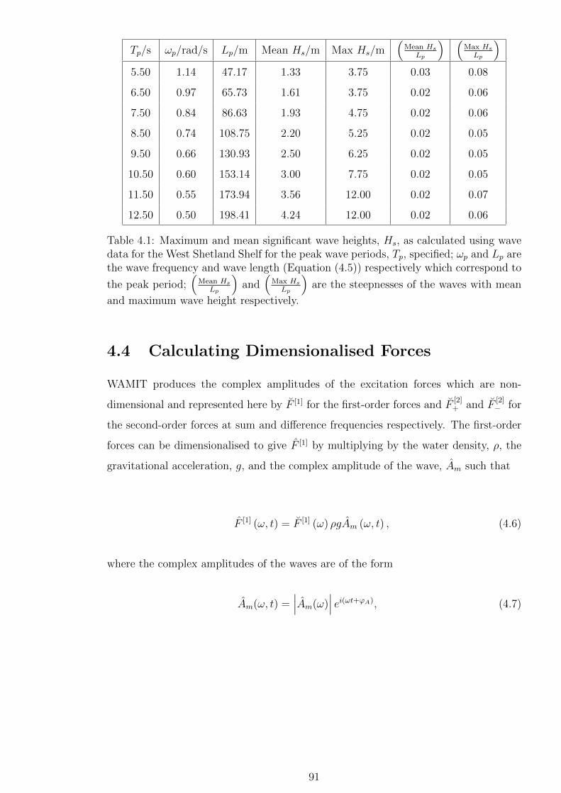
Tp/s ωp/rad/s Lp/m Mean Hs/m Max Hs/m(
Mean Hs
Lp
) (Max Hs
Lp
)
5.50 1.14 47.17 1.33 3.75 0.03 0.08
6.50 0.97 65.73 1.61 3.75 0.02 0.06
7.50 0.84 86.63 1.93 4.75 0.02 0.06
8.50 0.74 108.75 2.20 5.25 0.02 0.05
9.50 0.66 130.93 2.50 6.25 0.02 0.05
10.50 0.60 153.14 3.00 7.75 0.02 0.05
11.50 0.55 173.94 3.56 12.00 0.02 0.07
12.50 0.50 198.41 4.24 12.00 0.02 0.06
Table 4.1: Maximum and mean significant wave heights, Hs, as calculated using wavedata for the West Shetland Shelf for the peak wave periods, Tp, specified; ωp and Lp arethe wave frequency and wave length (Equation (4.5)) respectively which correspond to
the peak period;(
Mean Hs
Lp
)and
(Max Hs
Lp
)are the steepnesses of the waves with mean
and maximum wave height respectively.
4.4 Calculating Dimensionalised Forces
WAMIT produces the complex amplitudes of the excitation forces which are non-
dimensional and represented here by F [1] for the first-order forces and F[2]+ and F
[2]− for
the second-order forces at sum and difference frequencies respectively. The first-order
forces can be dimensionalised to give F [1] by multiplying by the water density, ρ, the
gravitational acceleration, g, and the complex amplitude of the wave, Am such that
F [1] (ω, t) = F [1] (ω) ρgAm (ω, t) , (4.6)
where the complex amplitudes of the waves are of the form
Am(ω, t) =∣∣∣Am(ω)
∣∣∣ ei(ωt+ϕA), (4.7)
91
where ϕA is the phase of the wave and |Am(ω)| its absolute amplitude. The second-order
forces can be dimensionalised by multiplying by ρ, g, the complex amplitude of the
first component wave and either the complex amplitude of the second component wave
for sum frequencies or its complex conjugate (denoted by ∗) for difference frequencies
such that
F[2]+ (ω1 + ω2, t) = F
[1]+ (ω1 + ω2) ρgAm (ω1) Am (ω2) (4.8)
and F[2]− (ω1 − ω2, t) = F
[1]− (ω1 − ω2) ρgAm (ω1) Am (ω2)∗ (4.9)
where, for difference frequencies, ω1 > ω2.
Selecting the phase at random such that 0 ≤ ϕA ≤ 2π, the dimensionalised complex
amplitudes of the excitation forces can be calculated for each frequency, ω, at a specific
time, t, using Equations (4.6), (4.8) and (4.9). The summation of these forces across the
frequency range then gives the excitation force at time t. Evaluation over 0 ≤ t ≤ tmax
yields a time series of the excitation force:
F[1]t (t) =
ωmax∑
ω=0
F (ω, t) (4.10)
F[2]t (t) =
max(ωi+ωj)∑
min(ωi+ωj)
F[2]+ (ωi + ωj, t) +
max(ωi−ωj)∑
min(ωi−ωj)
F[2]− (ωi − ωj, t) . (4.11)
A time series can be transformed back into the frequency domain using an FFT
(Fast Fourier Transform). The FFT is applied using Welch’s averaged modified pe-
riodogram method of spectral estimation, applied through the ‘Pwelch’ function in
MATLAB. Welch’s averaged modified periodogram method applies windows to the
time domain. The windows work as smoothing functions which weight the frequencies
so that peak in the middle of the window and decrease to zero at the edges. This
reduces the effects of any discontinuities which result from using a finite time signal.
The discontinuities are known as spectral leakage which primarily result from the finite
length of the time signal containing fractions of periods.
This results in the calculation of the spectral density of the first- and second-order
forces (ζ[1]F and ζ
[2]F respectively). The amplitudes of the dimensional second-order forces
are then obtained in the frequency domain from these force spectral densities using the
92

following equations:
∣∣F [1](ω)∣∣ =
√2ζ
[1]F (ω)δω (4.12)
∣∣F [2](ω)∣∣ =
√2ζ
[2]F (ω)δω. (4.13)
The resolution of the resultant spectrum is therefore dependent on the frequency
increment δω in Equations (4.12) and (4.13). It is however independent of δω in
Equation (4.3) allowing for a convergence in this parameter (section 4.5).
The process (Figure 4.1) of calculating the dimensional force spectrum from the
non-dimensional WAMIT forces and wave spectrum becomes
F (ω, t)→ F (t)→ ζF (ω)→ F (ω) (4.14)
for ω ∈ 0 : δω : ωmax and t ∈ 0 : δt : tmax.
Calculate the
wave amplitude
spectral density,
ζ(ω)
Calculate wave am-
plitudes, Am(ω),
from ζ(ω) using
Equation (4.3)
Calculate complex ampli-
tudes of non-dimensional
forces, F [1], F[2]+ and F
[2]− ,
using Wamit
Calculate frequency and time dependent dimensional forces,
F [1](ω, t), F[2]+ (ω, t) and F
[2]− (ω, t), for each time, t, and frequency,
ω using Equations (4.6), (4.8) and (4.9)
Create time series of dimensional forces, F[1]t (t) and F
[2]t (t), using
Equations (4.10) and (4.11)
Use Welch’s averaged modified periodogram method of spectral es-
timation to calculate the Force spectral densities, ζ[1]F (ω) and ζ
[2]F (ω)
Calculate the amplitude of the dimensional force in the frequency
domain,∣∣F [1](ω)
∣∣ and∣∣F [2](ω)
∣∣, from ζ[1]F (ω) and ζ
[2]F (ω) using Equa-
tions (4.12) and (4.13)
-
? ?
?
?
?
Figure 4.1: Flow chart showing process used to obtain dimensional excitation forceamplitudes in the frequency domain
93

4.5 Interpolation
As the calculation of second-order forces using WAMIT is computationally demanding,
the frequency range for which the non-dimensional forces are determined in WAMIT is
fairly coarse. For improved accuracy, it is desirable to use interpolated non-dimensional
forces to determine the dimensional forces. This section provides a convergence study
on the frequency increment to which the non-dimensional forces are interpolated. it is
necessary for the dimensional force amplitudes determined from the interpolated non-
dimensional forces to be independent of the choice of this frequency increment for the
first-order forces and converge for decreasing magnitude of this frequency increment
for the second-order forces.
Prior to interpolation, the non-dimensional force data is given in the frequency range
0.2 ≤ ω ≤ 2.8 rad/s with a frequency increment of 0.2 rad/sec (written 0.2 : 0.2 : 2.8
rad/s). The non-dimensional forces are interpolated to obtain data within the same
frequency range at finer frequency increments of δωint = 0.05, 0.01 rad/sec such that
the interpolated frequency range is 0.2 : δωint : 2.8 rad/s. The interpolation of the
non-dimensional forces is performed using a one-dimensional cubic interpolation for
the first-order forces and a two dimensional cubic interpolation for the second-order
forces since they are functions of one and two frequencies respectively (see Figures 4.2
and 4.3).
0 0.5 1 1.5 2 2.50
20
40
60
80
F [1]
ω
Figure 4.2: First-order non-dimensional wave forces, F [1], on a 2 × 1 array of hemi-spherical floats in head seas; The component waves are in the range 0.2 ≤ ω ≤ 2.8rad/s with the original data given at frequency increments of 0.2 rad/sec (crosses) andthe (cubic) interpolated data given at increments of 0.01 rad/sec (solid lines);KEY:Black, Front float (float 1); Grey, Back float (float 2)
94

01
23
01
230
5
10
ω1
ω2
F[2]+
(a) F[2]+ at original component frequencies (b) F
[2]+ at interpolated component frequencies
01
23
01
230
5
ω1
ω2
F[2]−
(c) F[2]− at original component frequencies (d) F
[2]− at interpolated component frequencies
Figure 4.3: Second-order non-dimensional wave forces, F[2]+ and F
[2]− , at the sum and
difference frequencies respectively of the component waves ω1 and ω2 on a 2×1 array ofhemispherical floats in head seas; The component waves are in the range 0.2 ≤ ω ≤ 2.8rad/s with the original data given at frequency increments of 0.2 rad/sec and the (cubic)interpolated data given at increments of 0.01 rad/sec; Solid vertical lines representω1 = ω2
A significant period of Ts = 6.14 seconds and a significant wave height of Hs = 3.75
m is used in Equation (4.2) to form the wave amplitude frequency spectrum (Figure
4.4a). The absolute amplitude of the waves is calculated from the spectral density (see
Figure 4.4b) using Equation (4.3) with δω = δωint such that
∣∣∣Am(ω)∣∣∣ =
√2ζ(ω)δωint. (4.15)
95

0 0.5 1 1.5 2 2.50
1
2
3
4
5
6
7
ζ
ω(a) Spectral density of wave amplitude
0 0.5 1 1.5 2 2.50
0.05
0.1
0.15
0.2
0.25
0.3
Am
ω(b) Wave amplitude calculated with
KEY Black, δω = δωint = 0.05 rad/sec;
Grey, δω = δωint = 0.01 rad/sec
Figure 4.4: The spectral density, ζ, of the wave amplitudes as calculated using theBretschneider spectrum with a significant period of Ts = 6.14 seconds; and a significantwave height of Hs = 3.75 m and the corresponding wave amplitudes, |Am|, on float2 calculated from the spectral density using Equation (4.3) with frequency incrementδω = δωint = 0.05 and 0.01 rad/sec
Using the process discussed in Section 4.4, the spectral densities, ζ[1]F and ζ
[2]F , of the
forces are determined. The amplitudes of the forces which can be obtained from these
force spectral densities is dependent on the frequency increment used within Equations
(4.12) and (4.13). In order to compare the forces obtained using different values of
δωint, the δω in Equations (4.12) and (4.13) must be constant and independent of
δωint. This constant value is δωF = 0.05 rad/s such that
∣∣F [1](ω)∣∣ =
√2ζ
[1]F (ω)δωF (4.16)
and∣∣F [2](ω)
∣∣ =
√2ζ
[2]F (ω)δωF . (4.17)
The terms ζ[1]F (ω)δωF and ζ
[2]F (ω)δωF in Equations (4.16) and (4.17) are achieved
using trapezoidal numerical integration of the spectral densities over frequency regions
of size δωF . The force spectral density must therefore be divided into discrete sections,
or bins, of size δωF .
The force spectral density is however created from the time series, which is created
from data at frequency increments of δωint. The force spectral density therefore already
contains frequency bins of width δωint centred on each of the frequencies in the range
0.2 : δωint : 2.8 rad/s (Figures 4.5a and 4.5b). These bins of width δωint must not be
divided when creating the bins of width δωF .
Where the desired frequency is ω, the corresponding bin of size δωF must therefore
96
be specified such that it contains frequencies ωj in the range
ωl1 ≤ ωj ≤ ωl2, (4.18)
where the limit frequencies are given by
ωl1 = (ω − 0.5δωF − 0.5δωint) (4.19)
and ωl2 = (ω + 0.5δωF − 0.5δωint) . (4.20)
In this way (Figure 4.5d) the original (pre-FFT) bins of size δωint are not subdivided (as
they are in Figure 4.5c), and the final bins are of size δωF regardless of the magnitude of
δωint. This allows the spectral densities formed using input data of different frequency
increments to be directly compared to each other. The horizontal centre of each such
bin of width δωF is then used as the output frequency, ωb, such that
ωb = ω − 0.5δωint (4.21)
which is close to, but not equal to the desired frequency, ω. The amplitudes of the
dimensionalised forces are therefore given by
∣∣F [1] (ωb)∣∣ =
√2
∫ ω2
ω1
ζ[1]F (ω)dω (4.22)
and∣∣F [2] (ωb)
∣∣ =
√2
∫ ω2
ω1
ζ[2]F (ω)dω (4.23)
where the integral is performed using the trapezoidal rule (as described in Appendix
E).
97
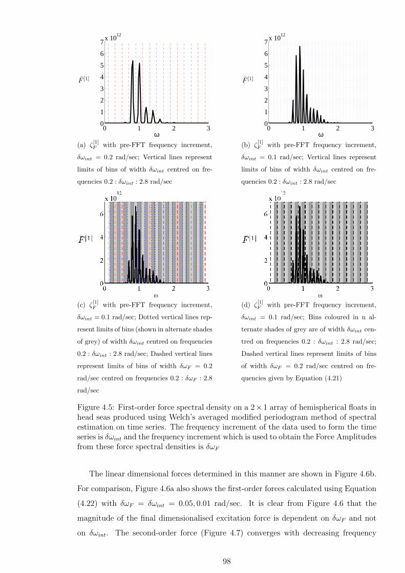
0 1 2 30
1
2
3
4
5
6
7x 10
12
ω
F [1]
(a) ζ[1]F with pre-FFT frequency increment,
δωint = 0.2 rad/sec; Vertical lines represent
limits of bins of width δωint centred on fre-
quencies 0.2 : δωint : 2.8 rad/sec
0 1 2 30
1
2
3
4
5
6
7x 10
12
ω
F [1]
(b) ζ[1]F with pre-FFT frequency increment,
δωint = 0.1 rad/sec; Vertical lines represent
limits of bins of width δωint centred on fre-
quencies 0.2 : δωint : 2.8 rad/sec
(c) ζ[1]F with pre-FFT frequency increment,
δωint = 0.1 rad/sec; Dotted vertical lines rep-
resent limits of bins (shown in alternate shades
of grey) of width δωint centred on frequencies
0.2 : δωint : 2.8 rad/sec; Dashed vertical lines
represent limits of bins of width δωF = 0.2
rad/sec centred on frequencies 0.2 : δωF : 2.8
rad/sec
(d) ζ[1]F with pre-FFT frequency increment,
δωint = 0.1 rad/sec; Bins coloured in n al-
ternate shades of grey are of width δωint cen-
tred on frequencies 0.2 : δωint : 2.8 rad/sec;
Dashed vertical lines represent limits of bins
of width δωF = 0.2 rad/sec centred on fre-
quencies given by Equation (4.21)
Figure 4.5: First-order force spectral density on a 2×1 array of hemispherical floats inhead seas produced using Welch’s averaged modified periodogram method of spectralestimation on time series. The frequency increment of the data used to form the timeseries is δωint and the frequency increment which is used to obtain the Force Amplitudesfrom these force spectral densities is δωF
The linear dimensional forces determined in this manner are shown in Figure 4.6b.
For comparison, Figure 4.6a also shows the first-order forces calculated using Equation
(4.22) with δωF = δωint = 0.05, 0.01 rad/sec. It is clear from Figure 4.6 that the
magnitude of the final dimensionalised excitation force is dependent on δωF and not
on δωint. The second-order force (Figure 4.7) converges with decreasing frequency
98

increment as required.
0 0.5 1 1.5 2 2.50
5
10
15x 10
4
F[1]
ω(a) Grey, δωint = δωF = 0.05 rad/s;
Black, δωint = δωF = 0.01 rad/s
0 0.5 1 1.5 2 2.50
0.5
1
1.5
2x 10
5
F[1]
ω(b) Solid line, δωint = δωF = 0.2 rad/s (origi-
nal WAMIT results without interpolation);
Grey o markers, δωint = 0.05 rad/s and δωF =
0.05 rad/s;
Black * markers, δωint = 0.01 rad/s and
δωF = 0.05 rad/s
Figure 4.6: First-order interpolated excitation force on front float of 2 × 1 array ofhemispherical floats, dimensionalised using amplitudes as given from Bretschneiderspectrum with significant period Ts = 6.14 seconds and significant wave height Hs =3.75 m; The WAMIT data is interpolated so that it is defined at frequency intervals ofδωint, transformed to a spectral density in the frequency domain using an FFT, thenevaluated at frequency intervals of δωF
0 0.5 1 1.5 2 2.50
2000
4000
6000
8000
F[2]±
ω
Figure 4.7: Second-order excitation force on front float of 2× 1 array of hemisphericalfloats calculated at both sum and difference frequencies; The WAMIT data is inter-polated so that it is defined at frequency intervals of δωint, transformed to a spectraldensity in the frequency domain using an FFT, then evaluated at frequency intervalsof δωFKEY:Grey, δωint = 0.05, rad/s δωF = 0.05 rad/s;Black, δωint = 0.01, rad/s δωF = 0.05 rad/s
99

The smallest increment of δωint = 0.01 is used to perform the second-order analysis
from herein as this results in the smoothest variation with frequency. The final incre-
ment from herein is small (δωF = 0.01) so as to achieve the greatest level of accuracy.
4.6 Variation of Forces with Hs and Tp
Interpolated forces are used in this section using WAMIT data with frequency incre-
ments of 0.2 rad/sec in the range 0.2 ≤ ω ≤ 2.8 rad/sec, and a frequency increment
of δωint = δωF = 0.01 rad/sec for the interpolated forces (see Section 4.5). A range of
different sea-states based on the Bretschneider spectrum (Equation (4.2)) are used to
determine the spectral density of the wave amplitudes by which the forces are dimen-
sionalised. Sea-states are defined with peak wave periods, Tp, in the range 5.5 - 12.5
seconds. For each peak period two significant wave heights, Hs, are considered based
on the mean and maximum heights that are predicted to occur for each period (see
4.3).
0.2 0.5 1.3 2.8
F
ω
maxF [1]
ω1ω2
Figure 4.8: Indicative graph showing variation with wave frequency of first-order forces(solid black line) and second-order forces (solid grey line) as dimensionalised using theBretschneider spectrum with frequencies in the range 0.2 ≤ ω ≤ 2.8 rad/sec for theback float (float 2) of a 2× 1 array of hemispherical floats in head seas; vertical dottedlines are shown to indicate the frequency range of interest to closely spaced arrays(0.5 ≤ ω ≤ 1.3 rad/sec); also shown are the maximum first-order force
(max
F [1])
and the frequencies ω1 and ω2 where F [2] > F [1] for ω ≤ ω1 < ωp and ωp ≤ ω2 < ω(where ωp = 2π
Tp)
The general trend of the first- and second-order dimensionalised forces is shown
in Figure 4.8. The first-order force forms a curve with a peak at a wave frequency
slightly less than the frequency corresponding to the peak wave period. This frequency
difference occurs since the non-dimensional force increases with decreasing wave fre-
quency. There is negligible energy content for frequencies that are less than ωp
2or
100

greater than 3ωp and hence first-order forces are also negligible over these ranges. The
second-order forces occur at the sum and difference frequencies of component waves.
The difference frequencies are therefore predominantly less than the peak frequency
and the sum frequencies greater than the peak frequency. Second-order forces are most
significant where the amplitudes of both component waves are large. This occurs when
both component wave frequencies are close to ωp, hence their sum is large and their
difference is small. Second-order forces are therefore of small magnitude close to the
peak frequency.
The frequency range over which the second-order force is greater than the first-
order force is identified as ω1 < ω < ω2 (see Figure 4.8). The values of ω1 and ω2 are
listed in Table 4.2 for all 16 of the sea states considered. The purpose of this chapter
is to determine whether second-order forces need to be considered when analysing
closely spaced arrays. The ratio of second to first-order forces in the likely operational
frequency range for closely spaced arrays of wave energy devices is therefore of most
importance. The maximum ratio of second-order forces to first-order forces within the
restricted frequency range of 0.5 ≤ ω ≤ 1.3 rad/sec (Section 1.2) is therefore shown
in Table 4.2. The frequency at which this maximum ratio occurs is called ωm. Only
frequencies for which the first-order forces are at least 1 % of the maximum first-order
force are considered within this range. This restriction eliminates excessively large
ratios of second to first-order forces at frequencies at which the first-order force is close
to zero. In particular, this restriction is applicable to low wave frequencies where the
peak period is low.
101
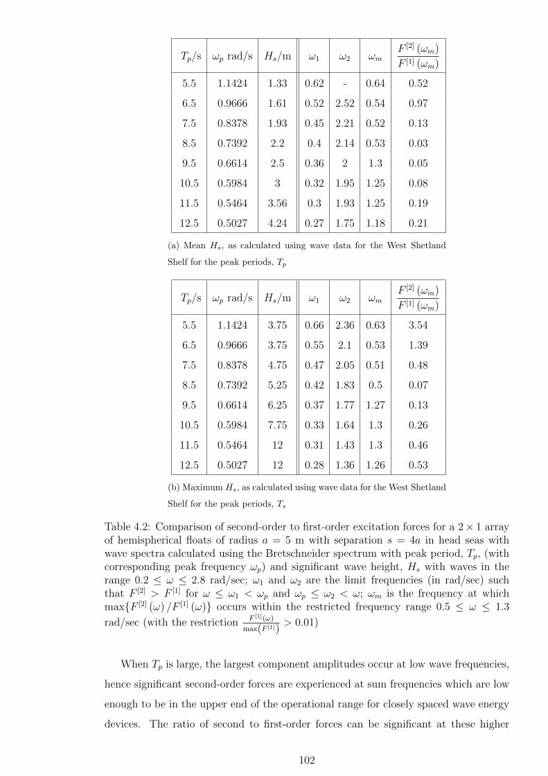
Tp/s ωp rad/s Hs/m ω1 ω2 ωmF [2] (ωm)
F [1] (ωm)
5.5 1.1424 1.33 0.62 - 0.64 0.52
6.5 0.9666 1.61 0.52 2.52 0.54 0.97
7.5 0.8378 1.93 0.45 2.21 0.52 0.13
8.5 0.7392 2.2 0.4 2.14 0.53 0.03
9.5 0.6614 2.5 0.36 2 1.3 0.05
10.5 0.5984 3 0.32 1.95 1.25 0.08
11.5 0.5464 3.56 0.3 1.93 1.25 0.19
12.5 0.5027 4.24 0.27 1.75 1.18 0.21
(a) Mean Hs, as calculated using wave data for the West Shetland
Shelf for the peak periods, Tp
Tp/s ωp rad/s Hs/m ω1 ω2 ωmF [2] (ωm)
F [1] (ωm)
5.5 1.1424 3.75 0.66 2.36 0.63 3.54
6.5 0.9666 3.75 0.55 2.1 0.53 1.39
7.5 0.8378 4.75 0.47 2.05 0.51 0.48
8.5 0.7392 5.25 0.42 1.83 0.5 0.07
9.5 0.6614 6.25 0.37 1.77 1.27 0.13
10.5 0.5984 7.75 0.33 1.64 1.3 0.26
11.5 0.5464 12 0.31 1.43 1.3 0.46
12.5 0.5027 12 0.28 1.36 1.26 0.53
(b) Maximum Hs, as calculated using wave data for the West Shetland
Shelf for the peak periods, Ts
Table 4.2: Comparison of second-order to first-order excitation forces for a 2× 1 arrayof hemispherical floats of radius a = 5 m with separation s = 4a in head seas withwave spectra calculated using the Bretschneider spectrum with peak period, Tp, (withcorresponding peak frequency ωp) and significant wave height, Hs with waves in therange 0.2 ≤ ω ≤ 2.8 rad/sec; ω1 and ω2 are the limit frequencies (in rad/sec) suchthat F [2] > F [1] for ω ≤ ω1 < ωp and ωp ≤ ω2 < ω; ωm is the frequency at whichmaxF [2] (ω) /F [1] (ω) occurs within the restricted frequency range 0.5 ≤ ω ≤ 1.3
rad/sec (with the restriction F [1](ω)
max(F [1])> 0.01)
When Tp is large, the largest component amplitudes occur at low wave frequencies,
hence significant second-order forces are experienced at sum frequencies which are low
enough to be in the upper end of the operational range for closely spaced wave energy
devices. The ratio of second to first-order forces can be significant at these higher
102

frequencies since the peak in the first-order wave force occurs at much lower wave
frequencies for high Tp values (Figures 4.9c, 4.9d, 4.10c and 4.10d). It is only when the
peak period is small (Figures 4.9a and 4.10a), that large magnitudes of second-order
forces occur at difference frequencies which are large enough to be within the range of
interest. When the peak period occurs such that the peak in the first-order force is
located in the middle of the frequency range of interest to closely spaced arrays, the
second-order forces are not significant in the same range (Figures 4.9b and 4.10b).
An increase in significant wave height causes an increase in the spectral density of
the component wave amplitudes. As the second-order forces are due to two component
waves but the first-order forces are a result of only one wave, this increase in spectral
density causes a more significant increase in the amplitudes of the second-order forces
than the first-order forces (Figure 4.9d and 4.10d).
For all sea states considered, the magnitude of the second order forces is small at all
wave frequencies when compared to the magnitude of the first order force at the peak
frequency. For the sea state with Tp = 12.5 seconds, ωp = 0.74 rad/sec and maximum
Hs (Hs = 12 m) for example (Figure 4.9b), the maximum second order force occurs
at ω = 2.18 rad/sec on both floats and is 5 and 6 % of the maximum first order force
(which occurs just lower than the peak frequency at ω = 0.69 rad/sec) on the first and
second order floats respectively.
103

0 0.5 1 1.5 2 2.50
0.02
0.04
0.06
0.08
0.1
0.12
Fn
ω(a) Tp = 5.5 seconds, Hs = maximum
0 0.5 1 1.5 2 2.50
0.02
0.04
0.06
0.08
0.1
0.12
Fn
ω(b) Tp = 8.5 seconds, Hs = maximum
0 0.5 1 1.5 2 2.50
0.02
0.04
0.06
0.08
0.1
0.12
Fn
ω(c) Tp = 12.5 seconds, Hs = mean
0 0.5 1 1.5 2 2.50
0.02
0.04
0.06
0.08
0.1
0.12
Fn
ω(d) Tp = 12.5 seconds, Hs = maximum
Figure 4.9: First- and second-order wave forces on the front float of a 2 × 1 array ofhemispherical floats in head seas. All forces are normalised by a fixed value which isthe maximum first-order force amplitude on an isolated hemispherical float, dimension-alised using wave amplitudes as calculated using the Bretschneider spectrum (Equation(4.2)) with significant wave period Ts = 0.95Tp and significant wave height, Hs
KEY:Black, First-order; Grey, Second Order
104
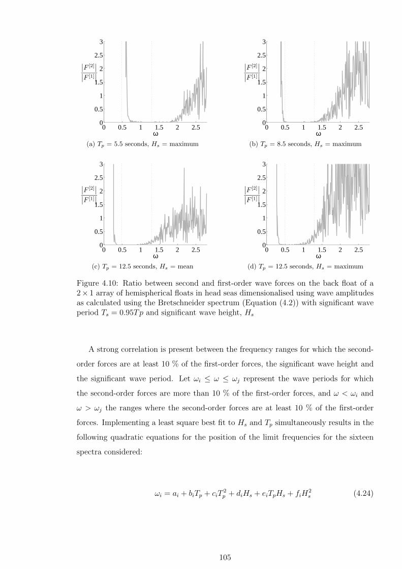
0 0.5 1 1.5 2 2.50
0.5
1
1.5
2
2.5
3
∣∣F [2]∣∣
∣∣F [1]∣∣
ω(a) Tp = 5.5 seconds, Hs = maximum
0 0.5 1 1.5 2 2.50
0.5
1
1.5
2
2.5
3
∣∣F [2]∣∣
∣∣F [1]∣∣
ω(b) Tp = 8.5 seconds, Hs = maximum
0 0.5 1 1.5 2 2.50
0.5
1
1.5
2
2.5
3
∣∣F [2]∣∣
∣∣F [1]∣∣
ω(c) Tp = 12.5 seconds, Hs = mean
0 0.5 1 1.5 2 2.50
0.5
1
1.5
2
2.5
3
∣∣F [2]∣∣
∣∣F [1]∣∣
ω(d) Tp = 12.5 seconds, Hs = maximum
Figure 4.10: Ratio between second and first-order wave forces on the back float of a2× 1 array of hemispherical floats in head seas dimensionalised using wave amplitudesas calculated using the Bretschneider spectrum (Equation (4.2)) with significant waveperiod Ts = 0.95Tp and significant wave height, Hs
A strong correlation is present between the frequency ranges for which the second-
order forces are at least 10 % of the first-order forces, the significant wave height and
the significant wave period. Let ωi ≤ ω ≤ ωj represent the wave periods for which
the second-order forces are more than 10 % of the first-order forces, and ω < ωi and
ω > ωj the ranges where the second-order forces are at least 10 % of the first-order
forces. Implementing a least square best fit to Hs and Tp simultaneously results in the
following quadratic equations for the position of the limit frequencies for the sixteen
spectra considered:
ωi = ai + biTp + ciT2p + diHs + eiTpHs + fiH
2s (4.24)
105
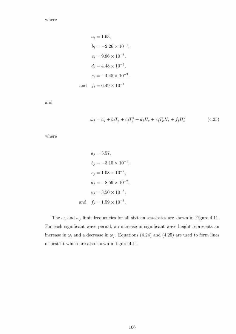
where
ai = 1.63,
bi = −2.26× 10⁻¹,
ci = 9.86× 10⁻³,
di = 4.48× 10⁻²,
ei = −4.45× 10⁻³,
and fi = 6.49× 10⁻⁴
and
ωj = aj + bjTp + cjT2p + djHs + ejTpHs + fjH
2s (4.25)
where
aj = 3.57,
bj = −3.15× 10⁻¹,
cj = 1.08× 10⁻²,
dj = −8.59× 10⁻²,
ej = 3.50× 10⁻³,
and fj = 1.59× 10⁻³.
The ωi and ωj limit frequencies for all sixteen sea-states are shown in Figure 4.11.
For each significant wave period, an increase in significant wave height represents an
increase in ωi and a decrease in ωj. Equations (4.24) and (4.25) are used to form lines
of best fit which are also shown in figure 4.11.
106
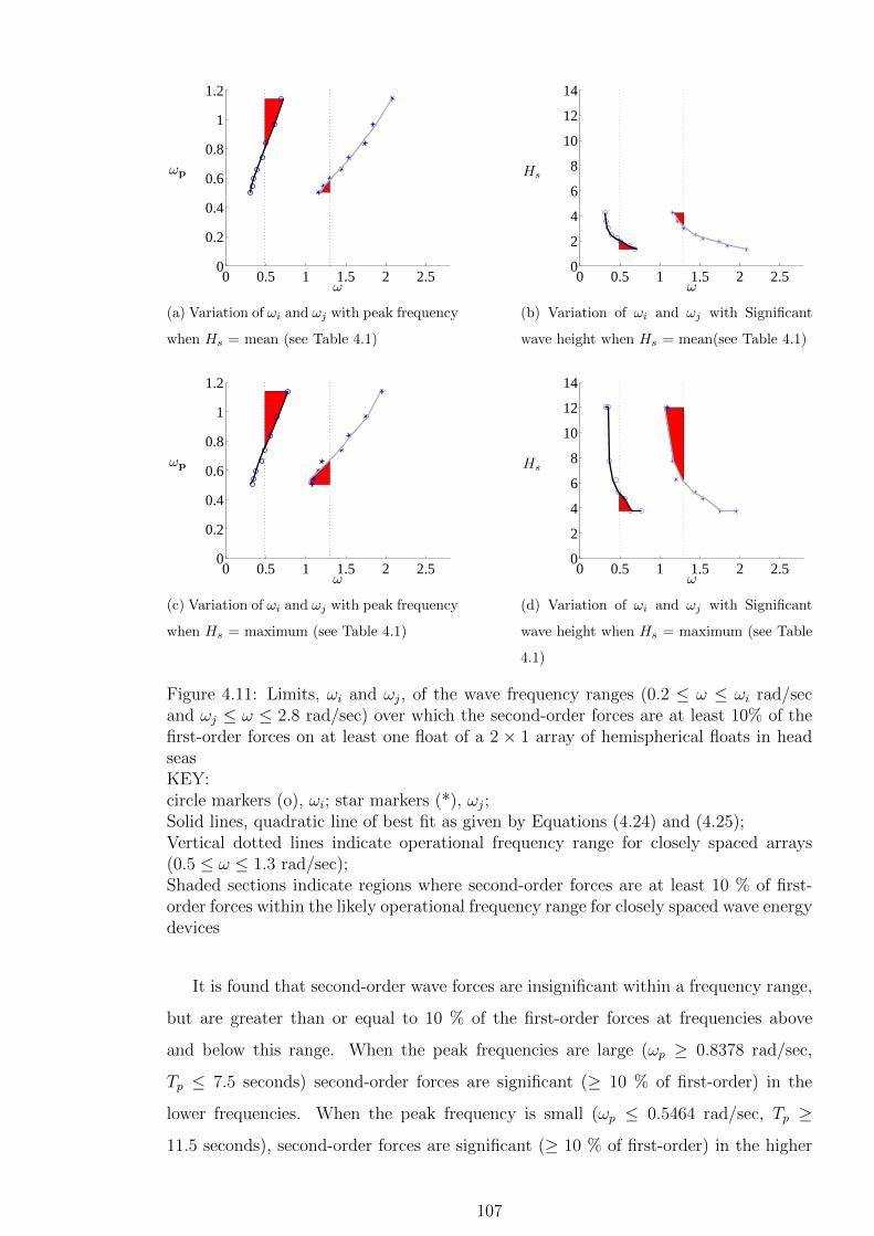
0 0.5 1 1.5 2 2.50
0.2
0.4
0.6
0.8
1
1.2
ωp
ω
(a) Variation of ωi and ωj with peak frequency
when Hs = mean (see Table 4.1)
0 0.5 1 1.5 2 2.50
2
4
6
8
10
12
14
Hs
ω
(b) Variation of ωi and ωj with Significant
wave height when Hs = mean(see Table 4.1)
0 0.5 1 1.5 2 2.50
0.2
0.4
0.6
0.8
1
1.2
ωp
ω
(c) Variation of ωi and ωj with peak frequency
when Hs = maximum (see Table 4.1)
0 0.5 1 1.5 2 2.50
2
4
6
8
10
12
14
Hs
ω
(d) Variation of ωi and ωj with Significant
wave height when Hs = maximum (see Table
4.1)
Figure 4.11: Limits, ωi and ωj, of the wave frequency ranges (0.2 ≤ ω ≤ ωi rad/secand ωj ≤ ω ≤ 2.8 rad/sec) over which the second-order forces are at least 10% of thefirst-order forces on at least one float of a 2 × 1 array of hemispherical floats in headseasKEY:circle markers (o), ωi; star markers (*), ωj;Solid lines, quadratic line of best fit as given by Equations (4.24) and (4.25);Vertical dotted lines indicate operational frequency range for closely spaced arrays(0.5 ≤ ω ≤ 1.3 rad/sec);Shaded sections indicate regions where second-order forces are at least 10 % of first-order forces within the likely operational frequency range for closely spaced wave energydevices
It is found that second-order wave forces are insignificant within a frequency range,
but are greater than or equal to 10 % of the first-order forces at frequencies above
and below this range. When the peak frequencies are large (ωp ≥ 0.8378 rad/sec,
Tp ≤ 7.5 seconds) second-order forces are significant (≥ 10 % of first-order) in the
lower frequencies. When the peak frequency is small (ωp ≤ 0.5464 rad/sec, Tp ≥11.5 seconds), second-order forces are significant (≥ 10 % of first-order) in the higher
107
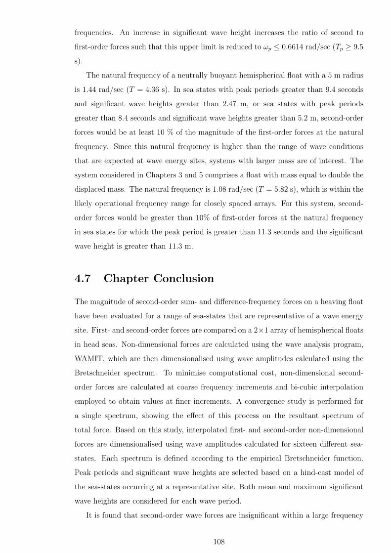
frequencies. An increase in significant wave height increases the ratio of second to
first-order forces such that this upper limit is reduced to ωp ≤ 0.6614 rad/sec (Tp ≥ 9.5
s).
The natural frequency of a neutrally buoyant hemispherical float with a 5 m radius
is 1.44 rad/sec (T = 4.36 s). In sea states with peak periods greater than 9.4 seconds
and significant wave heights greater than 2.47 m, or sea states with peak periods
greater than 8.4 seconds and significant wave heights greater than 5.2 m, second-order
forces would be at least 10 % of the magnitude of the first-order forces at the natural
frequency. Since this natural frequency is higher than the range of wave conditions
that are expected at wave energy sites, systems with larger mass are of interest. The
system considered in Chapters 3 and 5 comprises a float with mass equal to double the
displaced mass. The natural frequency is 1.08 rad/sec (T = 5.82 s), which is within the
likely operational frequency range for closely spaced arrays. For this system, second-
order forces would be greater than 10% of first-order forces at the natural frequency
in sea states for which the peak period is greater than 11.3 seconds and the significant
wave height is greater than 11.3 m.
4.7 Chapter Conclusion
The magnitude of second-order sum- and difference-frequency forces on a heaving float
have been evaluated for a range of sea-states that are representative of a wave energy
site. First- and second-order forces are compared on a 2×1 array of hemispherical floats
in head seas. Non-dimensional forces are calculated using the wave analysis program,
WAMIT, which are then dimensionalised using wave amplitudes calculated using the
Bretschneider spectrum. To minimise computational cost, non-dimensional second-
order forces are calculated at coarse frequency increments and bi-cubic interpolation
employed to obtain values at finer increments. A convergence study is performed for
a single spectrum, showing the effect of this process on the resultant spectrum of
total force. Based on this study, interpolated first- and second-order non-dimensional
forces are dimensionalised using wave amplitudes calculated for sixteen different sea-
states. Each spectrum is defined according to the empirical Bretschneider function.
Peak periods and significant wave heights are selected based on a hind-cast model of
the sea-states occurring at a representative site. Both mean and maximum significant
wave heights are considered for each wave period.
It is found that second-order wave forces are insignificant within a large frequency
108
range, but are greater than or equal to 10 % of the first-order forces at frequencies above
and below this range. Quadratic equations for the limit frequencies of the frequency
range over which second-order effects are less than 10 % of the first-order forces are
presented in terms of the significant wave height and the peak period. The operational
frequency range for closely spaced wave energy devices is limited. It is therefore only
when the peak period is either small or large that second-order effects are significant
(≥ 10 % of first-order) in the frequency range of interest for closely spaced arrays.
When the peak period is ≤ 7.5 seconds, second-order forces are significant in the lower
frequencies, and when the peak period is ≥ 11.5 seconds (or ≥ 9.5 seconds when
the significant wave height is large), second-order forces are significant in the higher
frequencies within the likely operational frequency range for closely spaced arrays.
109

Chapter 5
Optimisation of Fixed Geometry
Arrays
A numerical model in which the fluid is modelled using linear wave theory and the
wave energy devices are modelled as driven harmonic oscillators has been defined in
Chapter 2. The suitability of this model for predicting the response amplitude of
shallow draft floats arranged at close spacing was evaluated in Chapters 3 and 4.
The experimental comparison of Chapter 3 suggests the model provides a reasonable
prediction of response providing that response amplitudes are small. The second-order
force analysis of Chapter 4 suggests that, although second-order forcing does exist in
the frequency range of interest, it is small enough to exclude from the model without
loss of accuracy.
In this chapter the numerical model is used in order to determine appropriate values
for parameters that can feasibly be adjusted to modify the response of devices within
closely spaced arrays. The arrays considered are of fixed geometry and layout for all
wave frequencies considered and the objective is to select mechanical parameters such
that net power output from the array of devices is maximised.
5.1 Introduction
For an isolated device the time-averaged power output, P0, (where the suffix, 0, indi-
cates an isolated device), can be written using Equation (2.53) in which the velocity is
given by Equation (2.36) such that
110
P0 =1
2R
∥∥∥∥∥F (ω)
(R +B(ω)) + iω(M + A(ω)− S
ω2
)∥∥∥∥∥
2
. (5.1)
For a known wave frequency (ω) therefore, the power output P0 from an individual
device can be modified by changing the float form to adjust the excitation force, the
radiation damping, B, the added mass, A or the hydrodynamic stiffness, S. For a
float of predefined immersed geometry, as considered in this chapter, the power output
can only be modified by varying the float mass or the mechanical damping applied to
the float. The optimum power output for a fixed geometry float is given by applying
a mechanical damping equal to the radiation damping, R = B, and selecting a float
mass such that M = −A(ω) + Sω2 . A large variation of mass is not straightforward
to achieve however and, for the case of neutrally buoyant devices, a change of mass
would also result in a change of immersed geometry. It is possible to keep a constant
immersed geometry by using a float-counterweight-pulley system such as that described
in Section 3.
Within an array, the hydrodynamic terms (radiation damping and added mass) can
also be modified by altering the inter-float spacing and layout of the array. Several
studies have considered the influence of float spacing, configuration and array orien-
tation on power output. However, it will not necessarily be straightforward to alter
device spacing or array configuration during operation and so it is important to un-
derstand how the power output of arrays of predefined configuration can be modified.
Modification of power output by variation of immersed geometry of individual floats
is considered further in Chapter 6. In this chapter arrays of fixed float geometries in
fixed layouts are considered in which either the mechanical damping, R, or the total
mass of the floats, M , can be adjusted to achieve greater power. Although varying R is
not the most effective way to manipulate the power absorbed by an isolated device, it
may have a significant impact on the response and hence power within a closely spaced
array since the forcing on other floats due to radiated waves will be modified.
5.1.1 Optimising Array Power Output
A theoretical array which is optimally tuned would have frequency dependent mechan-
ical damping and mass specified such that R(ω) = B(ω) and M(ω) = Sω2 − A(ω),
however unlike for an isolated device this would require the use of dense matrices. The
off-diagonal elements of these matrices represent the application of an external force
111
to each float that is dependent on the velocity and acceleration of all other bodies
in the array and so are not straightforward to develop in a real system. This ide-
alised system is studied by (Fitzgerald and Thomas, 2007), (Falnes, 1980), (Thomas
and Evans, 1981) and (Mavrakos and McIver, 1997). For a linear array of five heav-
ing semi-immersed spheres of radius a in incident waves with wavenumber k = 0.4/a,
Fitzgerald and Thomas (2007) showed that a pentagonal configuration can attain an
interaction factor of up to q = 2.77. For the same device size and wavenumber but for
a linear array, which is the focus of this chapter, Thomas and Evans (1981) calculated
a maximum interaction factor of q = 2.25 over a range of device spacings. Whilst these
interaction factors are seemingly impressive, this requires specification of an external
force on each float that is a function of the motion of all other floats in the array. A
more easily implementable system is sought in this chapter in which the device spacing
does not need to be varied to match each incident wave frequency.
A more practical design approach would be to apply a certain amount of mass
and damping to each float irrespective of the motion of any other floats within the
array. A system in which the device spacing does not need to be varied to match each
incident wave frequency would also be more easily implementable. Several authors
have considered arrays with sub-optimal mechanical damping and mass matrices to
represent a feasible engineered system.
In regular seas, the diagonal mass and damping matrices which result in the greatest
net power have been sought by Justino and Clement (2003). The diagonal elements of
the matrices were defined by multiplying the diagonal elements of the corresponding
fully optimised dense matrices by constant values within the range 0.8 to 1.2. They
determined that when calculating diagonal R and M matrices in this manner, the
greatest power could be achieved by using constant value of 1. In order to achieve
the greatest power in different irregular wave spectra, sub-optimal diagonal damping
matrices were iteratively selected for a fixed mass array by Cruz et al. (2009) and sub-
optimal diagonal damping and mass matrices were selected by de Backer et al. (2009)
using the theory of linear superposition. Greater interaction factors were found when
each diagonal element of the damping matrix was selected individually than if they
were all set to be equal to one value (either selected to give greatest power or set equal
to the radiation damping of an isolated device).
The purpose of this chapter is to calculate the greatest power which can be achieved
in regular seas by a sub-optimal closely-spaced array whose mass and mechanical damp-
ing arrays are diagonal matrices. The effects in irregular waves are not considered here
112

as it remains unclear whether superposition of interaction factors derived assuming
steady state response is a valid approach. A 5 × 1 array of semi-immersed spheres of
radius a whose masses are constant and equal to twice the displaced mass of the water
is considered with centre to centre separation distances of s = 4a and a water depth
of d = 7a. The two incident wave train directions, beam and head seas, are shown in
diagram 5.1 together with the float numbering.
Figure 5.1: Diagram of 5× 1 array of hemispheres of radius a with a centre to centreseparation distance of s = 4a; beam and head sea directions are also indicated
The influence of the form of the mass and damping matrices on power output and
interaction factor is shown in Section 5.2. Methods to calculate the optimum diagonal
mechanical damping elements are explained in Section 5.4. An iterative method to
select the diagonal matrix elements is described in Section 5.3. The result of using the
iterative method to select the diagonal elements of the mechanical damping and mass
matrices is then discussed in Sections 5.5 and 5.6 respectively.
5.2 Basic Approaches to Selecting Diagonal M and
R Matrices
The system mass matrix, M , (which excludes the added mass, A) and the mechanical
damping matrix, R, can be varied in order to manipulate the net power from an array.
When both the optimum dense mass and optimum dense damping matrices are used
such that the net power can be calculated using Equation (2.54), the net power, and
hence Q is maximised at all wave frequencies (thin dotted line in Figure 5.2b). In
practice, a dense mass matrix is difficult to achieve since the off-diagonal elements of
the mass matrix represent a force that is dependent on the acceleration of all floats.
This section considers several methods for calculating diagonal mass and damping
matrices and evaluates the influence of these diagonal matrices on the response of
a closely spaced line array of five devices. Both the interaction factor, q, and the
Normalised interaction factor, Q, are shown in Figure 5.2 for five element arrays in
which the mass and mechanical damping matrices are varied. The relevant isolated
113
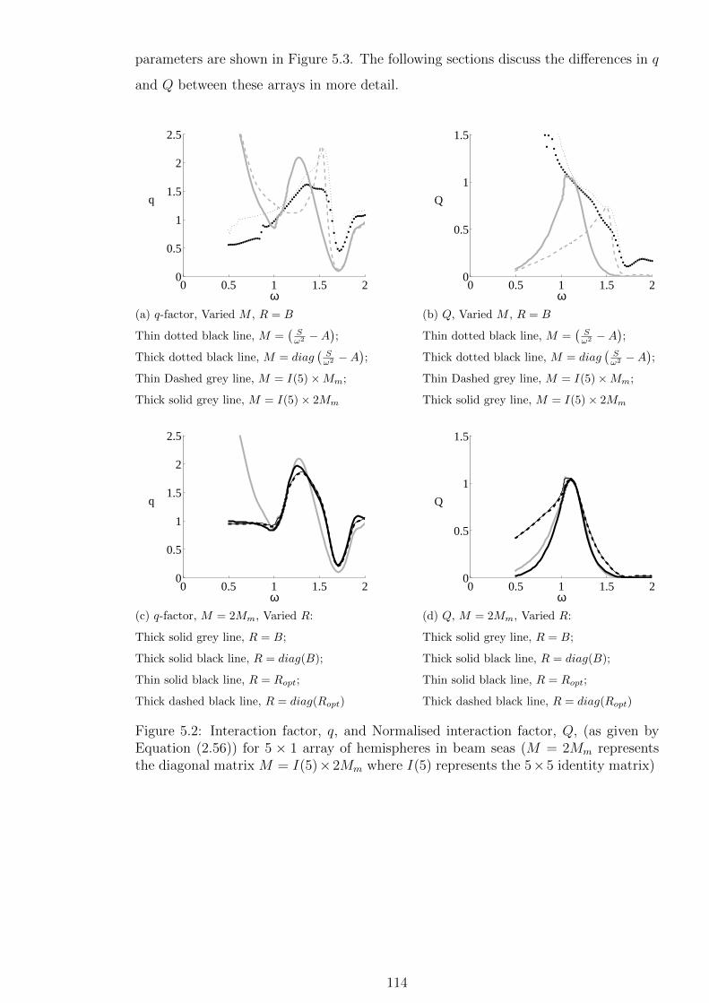
parameters are shown in Figure 5.3. The following sections discuss the differences in q
and Q between these arrays in more detail.
0 0.5 1 1.5 20
0.5
1
1.5
2
2.5
q
ω(a) q-factor, Varied M , R = B
Thin dotted black line, M =(
Sω2 −A
);
Thick dotted black line, M = diag(
Sω2 −A
);
Thin Dashed grey line, M = I(5)×Mm;
Thick solid grey line, M = I(5)× 2Mm
0 0.5 1 1.5 20
0.5
1
1.5
Q
ω(b) Q, Varied M , R = B
Thin dotted black line, M =(
Sω2 −A
);
Thick dotted black line, M = diag(
Sω2 −A
);
Thin Dashed grey line, M = I(5)×Mm;
Thick solid grey line, M = I(5)× 2Mm
0 0.5 1 1.5 20
0.5
1
1.5
2
2.5
q
ω(c) q-factor, M = 2Mm, Varied R:
Thick solid grey line, R = B;
Thick solid black line, R = diag(B);
Thin solid black line, R = Ropt;
Thick dashed black line, R = diag(Ropt)
0 0.5 1 1.5 20
0.5
1
1.5
Q
ω(d) Q, M = 2Mm, Varied R:
Thick solid grey line, R = B;
Thick solid black line, R = diag(B);
Thin solid black line, R = Ropt;
Thick dashed black line, R = diag(Ropt)
Figure 5.2: Interaction factor, q, and Normalised interaction factor, Q, (as given byEquation (2.56)) for 5 × 1 array of hemispheres in beam seas (M = 2Mm representsthe diagonal matrix M = I(5)×2Mm where I(5) represents the 5×5 identity matrix)
114
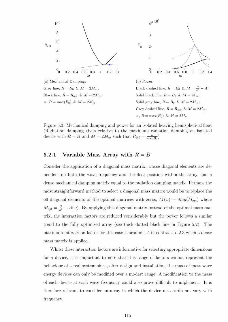
0 0.2 0.4 0.6 0.8 1 1.2 1.40
2
4
6
8
10
RB0
ω(a) Mechanical Damping:
Grey line, R = B0 & M = 2Mm;
Black line, R = Ropt & M = 2Mm;
×, R = max(B0) & M = 2Mm
0 0.2 0.4 0.6 0.8 1 1.2 1.40
1
2
3
4x 10
5
P0
ω(b) Power:
Black dashed line, R = B0 & M = Sω2 −A;
Solid black line, R = B0 & M = Mm;
Solid grey line, R = B0 & M = 2Mm;
Grey dashed line, R = Ropt & M = 2Mm;
×, R = max(B0) & M = 2Mm
Figure 5.3: Mechanical damping and power for an isolated heaving hemispherical float(Radiation damping given relative to the maximum radiation damping on isolateddevice with R = B and M = 2Mm such that RB0 = R
maxB0)
5.2.1 Variable Mass Array with R = B
Consider the application of a diagonal mass matrix, whose diagonal elements are de-
pendent on both the wave frequency and the float position within the array, and a
dense mechanical damping matrix equal to the radiation damping matrix. Perhaps the
most straightforward method to select a diagonal mass matrix would be to replace the
off-diagonal elements of the optimal matrices with zeros, M(ω) = diag(Mopt) where
Mopt = Sω2 − A(ω). By applying this diagonal matrix instead of the optimal mass ma-
trix, the interaction factors are reduced considerably but the power follows a similar
trend to the fully optimised array (see thick dotted black line in Figure 5.2). The
maximum interaction factor for this case is around 1.5 in contrast to 2.3 when a dense
mass matrix is applied.
Whilst these interaction factors are informative for selecting appropriate dimensions
for a device, it is important to note that this range of factors cannot represent the
behaviour of a real system since, after design and installation, the mass of most wave
energy devices can only be modified over a modest range. A modification to the mass
of each device at each wave frequency could also prove difficult to implement. It is
therefore relevant to consider an array in which the device masses do not vary with
frequency.
115
5.2.2 Fixed Mass Array with R = B
Consider now the application of a diagonal mass matrix, whose diagonal elements are
constant, and a dense mechanical damping matrix equal to the radiation damping ma-
trix. Interaction factors are shown for two fixed mass systems in Figure 5.2 representing
an array of neutrally buoyant floats (M = Mm) with R = B and an array of floats of
double this mass (M = 2Mm) and R = B. This represents a system in which each
float is connected to a supplementary mass as considered by (Stallard et al., 2009a)
and (de Backer et al., 2009). Clearly the fixed and variable mass systems exhibit very
different interaction factor trends to each other. At their maxima, the q-factors for
fixed mass arrays exceed the optimal system at the same frequency, particularly for
the heavier constant mass (thick solid grey line). It is important to note that this only
occurs because the factors are defined relative to the same device in isolation; for the
optimal array, the isolated device mass varies with frequency whereas for the constant
mass array the isolated device has constant mass.
The increase in mass from Mm to 2Mm significantly reduces the wave frequency
at which the peak in net power occurs. For typical hemispherical floats of radius 5
m, float masses of 1.88Mm ≤ M ≤ 11.76Mm would put the natural frequency of the
floats within the desired frequency range 0.5 to 1.25 rad/sec (as discussed in Section
1.2), however from an engineering perspective it is desirable for the masses to be as
small as possible. Small mass systems are generally advantageous since this reduces
cost, particular of installation and, in the case of structure supported devices, reduces
structural requirements. Herein an array of equal mass floats of mass 2Mm is considered
in which each float drives an independent linear damper which applies a force in phase
with the velocity of that float only. The mass and mechanical damping matrices are
therefore both diagonal, with all of the diagonal elements of the mass matrix equal to
2Mm at all wave frequencies. For this system, it is not straightforward to determine
the mechanical damping for each float that would maximise net power output from the
array of floats. Approaches based on the radiation damping matrix and an iterative
method are considered.
5.2.3 Fixed Mass Array with R = diag(B)
Consider now the application of a diagonal mass array with constant diagonal values,
together with a diagonal mechanical damping matrix. Perhaps the most straight-
forward selection of a diagonal mechanical damping matrix is to apply the diagonal
116

elements of a dense damping matrix, R = diag(B). A similar approach has been inves-
tigated by Justino and Clement (2003) who showed that application of the diagonal of
the intrinsic impedance matrix (B+ iω(M +A)) maximised the power output from an
array of fully-immersed spheres for a given wave frequency. This approach can only be
applied if both mass and damping are modified with wave frequency. A similar anal-
ysis, but with constant mass, M = 2Mm, and different range of constant multiplier
values is shown here in Figure 5.4 for a 5× 1 array of heaving, semi-immersed spheres
in beam seas. A similar conclusion to Justino and Clement (2003) can be drawn in that
maximum power is obtained from this fixed mass array by applying a diagonal damping
matrix whose elements are all exactly equal to the radiation damping elements.
0.6 0.8 1 1.2 1.40
0.5
1
1.5
ω
Figure 5.4: Comparison of Pnet values obtained for a 5 × 1 array of hemispheres inbeam seas by varying the choice of R matrix such that either R = diag (Ropt) orR = γ4diag(B) for different values of constant γ4:KEY:Thick dashed line, R = diag (Ropt); Thick dotted line, R = 5diag(B); Solid grey line,R = 3diag(B); Solid black line, R = diag(B); Thin dashed line, R = 0.5diag(B)
5.2.4 Fixed Mass Array with R = diag(Ropt)
An alternative approach to select the diagonal elements of the mechanical damping
matrix is based on the output of an isolated device. Equation 5.1 gives the power
which can be absorbed by a mechanical damper applying a damping force R to an
isolated device. The differential with respect to R of equation 5.1 can be equated with
zero to determine Ropt; the value of R which results in the greatest power for an isolated
device (equation 5.2) (Falnes, 1980).
Ropt =
√B2 + ω2
(A+M − S
ω2
)2
(5.2)
By substituting matrices A, B, M and S to equation 5.2 in place of the intended scalars
a (nearly) optimum dense damping matrix can be obtained for an array. This approach
117

is not expected to give the maximum attainable power output but does account for use
of a fixed mass matrix.
5.2.5 Comparison of Fixed Mass Arrays with R = diag(B) and
R = diag(Ropt)
0 0.2 0.4 0.6 0.8 1 1.2 1.40
0.2
0.4
0.6
0.8
1
1.2
RB0
ω(a) R = diag(B)
0 0.2 0.4 0.6 0.8 1 1.2 1.40
1
2
3
4
RB0
ω(b) R = diag (Ropt)
Figure 5.5: Mechanical damping, R, calculated as R = diag(B) and R = diag (Ropt)and normalised by the maximum radiation damping on the isolated hemisphere(max(B0)) for a 5× 1 array of hemispheres in beam seas:KEY:Solid black line, float 1 (and 5); Solid grey line, float 2 (and 4); Dashed line, float 3;Grey circular markers = damping on isolated device
.
Figure 5.5 shows the frequency variation of both R = diag(B) and R = diag(Ropt) for
each element of a 5×1 beam seas array, together with the damping on an isolated device
such that R = B and R = Ropt respectively. The elements of the damping matrices
follow a similar trend to the damping on the isolated device, however a greater variation
in damping can be seen in the array with R = diag(B). The two damping matrices
(and isolated damping curves) have opposing trends with wave frequency.
Applying the damping matrices R = diag(Ropt) or R = diag(B) to the arrays results
in net powers and hence Q which form a parabola when plotted against frequency (as
shown in Figure 5.2) with a peak at ω = 1.1 rad/sec in beam seas and ω = 1.02 rad/sec
in head seas. At frequencies away from the peak, the damping matrix R = diag(Ropt)
results in a greater net power than R = diag(B). At frequencies near the peak in beam
seas both matrices result in an equal net power whereas in head seas R = diag(B)
results in a greater net power than R = diag(Ropt).
Interaction factors resulting from these mechanical damping configurations are also
shown in Figure 5.2. Note that these are normalised to a different isolated device, with
118

the interaction factors for arrays with R = diag(Ropt) and R = diag(B) calculated
relative to an isolated device whose mechanical damping values are given by R = Ropt
(by applying Equation (5.2)) and R = B respectively.
Applying the R = diag(B) and R = diag(Ropt) damping values to the array in beam
seas results in an interaction factor greater than one (indicating positive interaction)
for 1.062 ≤ ω ≤ 1.57 rad/sec and 1.06 ≤ ω ≤ 1.59 rad/sec respectively and also for
very high frequencies. In head seas the resulting interaction factors are predominantly
below 1 (indicating negative interaction within the array) for all frequencies with R =
diag(Ropt) and higher frequencies (ω ≥ 1.032 rad/sec) with R = diag(B).
Within the range of interest for closely spaced arrays (0.5 ≤ ω ≤ 1.25 rad/sec)
therefore, positive interaction is seen in beam seas only for high frequencies (1.06 ≤ω ≤ 1.25 rad/sec) for arrays with either R = diag(B) or R = diag(Ropt), and in head
seas only for the array with R = diag(B) for 0.49 ≤ ω ≤ 1.032 rad/sec.
It is unclear whether either of these diagonalisation approaches yield the maximum
net power output from the array and so it is useful to determine whether float-specific
values of mechanical damping can improve power output.
5.3 Diagonal Damping Matrix Selection Procedure
In this Section, unique damping values are identified for each float such that the net
power output from the array is maximised. To individually select the diagonal elements
of the diagonal mechanical damping matrix, R, which will result in the greatest net
power, two different methods are applied and compared for a discrete range of wave
frequencies, ω. Both methods produce similar damping values to each other with the
resulting net power values within 0.6 % of each other. Both methods are described
here in detail.
5.3.1 Method 1
A discrete range of possible R values is defined and at each wave frequency the net
powers resulting from applying every combination of these values as diagonal elements
of the R matrix is calculated (as shown in Figure 5.6 for a 2-element array). At each
wave frequency the combination which results in the greatest net power is selected
(as shown by the circular markers in Figure 5.6 for a 2-element array). For a two-
119
element array this method allows a visual representation of the power attainable from
all possible combinations of damping values showing that there is only one peak in
power at each wave frequency (Figure 5.6). The uniqueness of the selected optimal
damping values cannot be visualised for larger arrays however.
Using this method, the damping values are selected in a clear manner, however the
computational cost is high and so the size of the discrete range of wave frequencies
and possible R values are limited by the computational memory. Using a computer
with a 3.19 GHz Processor and 2 GB RAM, the optimal damping matrix for a two
element array can be calculated in 61 seconds from a range of 500 damping values,
and 272 seconds from a range 1000 damping values. For a larger, N -element array the
number of required calculations at each wave frequency would be increased from (NR)2
to (NR)N where NR is the number of damping values considered.
120
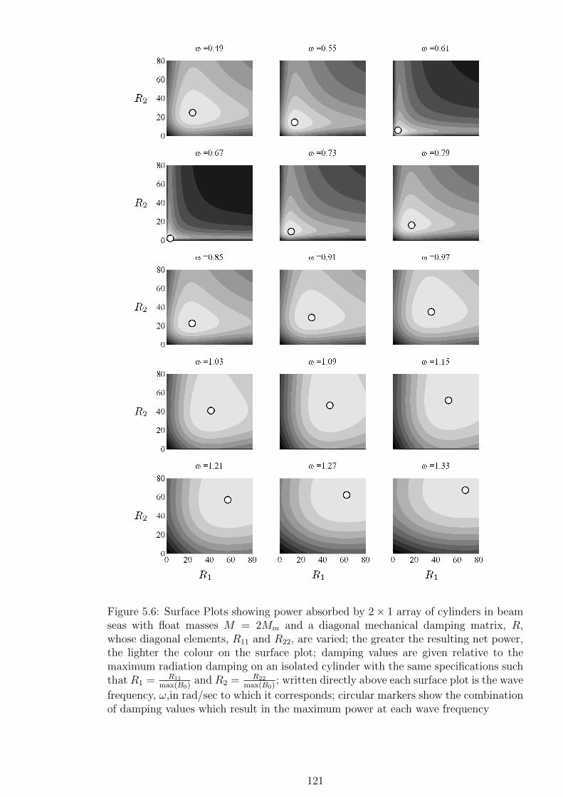
Figure 5.6: Surface Plots showing power absorbed by 2× 1 array of cylinders in beamseas with float masses M = 2Mm and a diagonal mechanical damping matrix, R,whose diagonal elements, R11 and R22, are varied; the greater the resulting net power,the lighter the colour on the surface plot; damping values are given relative to themaximum radiation damping on an isolated cylinder with the same specifications suchthat R1 = R11
max(B0)and R2 = R22
max(B0); written directly above each surface plot is the wave
frequency, ω,in rad/sec to which it corresponds; circular markers show the combinationof damping values which result in the maximum power at each wave frequency
121

5.3.2 Method 2
The second method is an iterative method which uses an inbuilt MATLAB function
to apply the Levenberg-Marquardt algorithm. A discrete range of net power values
is specified, and the algorithm is applied to determine the values of R and individual
power values from continuous domains which result in net power to within 10−10 of the
specified net power. The greatest net power value at each ω for which R values are
obtained is then stored.
The Levenberg-Marquardt algorithm is a least squares algorithm which uses an iter-
ative approach to determine the mechanical damping values. Whilst Method 1 requires
the calculation of power for every combination of damping values in the specified fre-
quency range, Method 2 calculates only the values which it determines necessary using
the least squares approach. The computational cost of Method 2 is therefore much
less than method 1 allowing for an application to a much wider range of mechanical
damping values (an infinite range) and application to more wave frequencies.
To minimise computational time, the iterative procedure is first run with a large
but coarse net power range of 0.4 max(Pnet(R = diag(B))) ≤ Pnet ≤ 1.3 max(Pnet(R =
diag(B))) with 100 power increments (I = 0.9 max(P0)/100) within this range. At
each wave frequency, ω, the maximum net power from this range for which R values
are determined is called P1(ω). The iterative procedure is then completed for a second
time using the results of the first iterative procedure such that the discrete power range
is reduced to P1(ω) ≤ Pnet ≤ (P1(ω) + 4I) with 400 finer increments in this range. The
mechanical damping values selected in the initial iterative procedure are used as initial
values in the second iterative procedure.
The entire procedure to determine the optimal diagonal mechanical damping matrix
is therefore given by
1 A discrete coarse range of net power values, P[C]net , is specified as 0.4 max(Pnet(R =
diag(B))) ≤ Pnet ≤ 1.3 max(Pnet(R = diag(B))) with 100 power increments
(I = 0.9 max(P0)/100) within this range
2 At each ω,
(a) For each Pnet ∈ P [C]net , elements of R and individual power values from con-
tinuous domains which result in net power values within 9 decimal places
of Pnet are obtained using the Levenberg-Marquardt algorithm. The initial
starting value for each R element is the maximum radiation damping on an
122

isolated device, max (B0), and the initial starting value of each individual
power value is Pnet
Nwhere N is the number of elements within the array.
(b) The greatest Pnet value for which R values are obtained is then stored and
called P1(ω), and the corresponding vectors of R and individual power values
are called R1it(ω) and P1it(ω) respectively.
(c) A finer discrete range of net power values, P[F ]net , is specified as P1(ω) ≤
Pnet ≤ (P1(ω) + 4I) with 400 finer increments in this range
(d) For each Pnet ∈ P [F ]net , elements of R and individual power values from con-
tinuous domains which result in net power values within 9 decimal places
of Pnet are obtained using the Levenberg-Marquardt algorithm. The ini-
tial starting values for the R elements are given by R1it(ω), and the initial
starting values of the individual power values are given by P1it(ω).
(e) The greatest Pnet value for which R values are obtained is then stored to-
gether with the corresponding optimal diagonal R matrix.
The iterative method is restricted by the discrete range of net power values for
which damping values are sought. As a result, float-specific values are determined
within the range 0.49 ≤ ω ≤ 1.35 and so covers a representative range of operational
wave conditions, as outside of this range lower net power values are required.
5.3.3 Comparison of Methods
The two methods are compared in this section for a two element array of cylindrical
floats (represented by the surface plot in Figure 5.6 for Method 1) and a five element
array of hemispherical floats for the frequency range, 0.49 ≤ ω ≤ 2.3 rad/sec with
increments of 0.02 rad/sec.
For the two element array, the frequency range over which a large amount of power
is absorbed by the array (the bandwidth) is small. If Method 2 is applied by considering
net power values which are at least 40 % of the maximum net power achieved when
R = diag(B) as defined in Section 5.3.2, suitable damping values are only attained
for the peak frequency (ω = 0.65 rad/sec) and directly adjecent frequencies (ω = 0.63
and 0.67 rad/sec). In order to increase the range of frequencies over which the two
methods can be compared, net powers are sought instead which are at least 10 % of
the maximum net power achieved when R = diag(B). With this increased range of
net power values considered, Method 2 determines suitable damping matrices for all
frequencies in the range 0.49 ≤ ω ≤ 0.75 rad/sec.
123
The same net power is calculated using both methods (less than 0.1 % difference)
at all frequencies except the peak frequency. The net power determined using method
2 however is 2 % less than that determined using method 1 at the peak frequency
(ω = 0.65 rad/sec).
The mechanical damping values which are selected using each method follow the
same trend (Figure 5.7a). The damping values selected, however, do vary by up to 110
% at the peak frequency and 6 % at all other frequencies. The damping values selected
by both methods are minimal on both floats at the peak frequency. The variation in
damping values of 110 % between methods at the peak frequency therefore corresponds
to only a small variation in magnitude of damping.
When the damping and power values selected by Method 2 are set as initial values
for the iterative procedure of Method 1, damping values are determined which result
in 0.3 % greater net power than that determined by Method 2. This corresponds to an
increase of 2.5 % compared to the net power determined using the generic initial values
as specified in Section 5.3.2. Although there exists a clear dependence of Method 2 on
the initial values, a descrepency below 3 % it is not considered significant enough to
void its results.
The computational time to compute the optimal diagonal mechanical damping ma-
trix using method 1 is 40 % greater than that of method 2 for the two-element array.
For larger arrays the computational inefficiency of Method 1 makes it unrealistic for
it to be used to determine the initial conditions for Method 2. Although there exists
a clear dependence of Method 2 on the initial values, it is able to produce similar net
power values to Method 1 when using generic initial values with significantly reduced
computational time.
The two methods are compared for a 5 × 1 array of hemispherical floats in beam
seas. For the purpose of comparison, additional conditions are placed in Method 2 to
restrict the discrete R range such that 0.5 max(B0) ≤ Ri,i ≤ 8 max(B0). As with the
two element array, the mechanical damping values selected using both methods in order
to achieve greatest power are found to follow the same trend. As the range of R values
is discrete in the first method and continuous in the second method, different damping
values are determined with each method although this is less than 7.2 % difference for
all but one frequency. The difference in the resulting net power values however is found
to be less than 0.6 % for all wave frequencies.
In order to allow for efficient analysis of arrays of five or more bodies, Method 2 is
used from herein to determine the optimal diagonal damping matrices.
124

0 0.2 0.4 0.6 0.8 10
10
20
30
40
R
max(B0)
ω(a) Mechanical damping
(Black, float 1; Grey, float 2)
0 0.2 0.4 0.6 0.8 10
0.2
0.4
0.6
0.8
1
1.2
Q
ω(b) Q-factor
Figure 5.7: Elements of the optimal diagonal mechanical damping matrix elements rel-ative to the maximum radiation damping on an isolated device and their correspondingoptimal Q-factors (determined using Equation (2.56) where the isolated body has thesame specifications as the bodies within the array) for a 2×1 array of cylindrical floatswith radius = draft = a = 5 m, s = 4a, and M = 2Mm
KEY:Dotted lines, Method 1 (see Section 5.3.1); Solid lines, Method 2 (see Section 5.3.2)
If there is only one peak value then it could be possible to differentiate the power
equation with respect to matrix R in order to determine the optimal mechanical damp-
ing matrix. The method of differentiation is discussed further in the next section.
5.4 Direct Sub-Optimal R Matrix Calculation
For an isolated device, the mechanical damping value which will result in the greatest
power is given by Ropt (Equation (5.2)) which is identified as the zero of the differential
of power with respect to mechanical damping (dP0
dR= 0). Theoretically, the same
method could be used to determine the mechanical damping matrix which will result
in the greatest power from an array of devices by differentiating Equation (2.49) with
respect to the matrix R and equating with zero. This procedure is discussed in this
section.
Prior to differentiation of Equation (2.49) the velocity given by Equation (2.36)
must be substituted into (2.49). This must then be expanded using the rules of complex
matrix multiplication to give power, P , in terms of the matrices constituent elements,
Ri,j, Bi,j, Ai,j, Si,i, Mi,i, <Fi, =Fi as well as ω.
Using the chain rule P can be written as:
125
dP
dR=∂P
∂U
∂U
∂R. (5.3)
P is a single value and U a vector, so the first partial differential equation can be
written as
∂P
∂U=[
∂P∂U1
∂P∂U2
· · ·]. (5.4)
U is a vector and R a matrix, so the second partial differential in Equation (5.3) can
be written as
∂U
∂R=
∂U∂R11
∂U∂R21
· · ·∂U∂R12
∂U∂R22
· · ·...
......
. (5.5)
Using Equations (5.3) together with Equations (5.4) and (5.5) therefore gives
dP
dR=[ (
∂P∂U1
∂U∂R11
+ ∂P∂U2
∂U∂R12
+ · · ·)
,(∂P∂U1
∂U∂R21
+ ∂P∂U2
∂U∂R22
+ · · ·)
, · · ·]. (5.6)
Both the net power, P , given by Equation (2.49) and the velocity, U , given by Equation
(2.36) are complex. The differentiation is therefore further complicated by the differen-
tials of complex numbers. The Cauchy-Riemann Formula for the derivative of a com-
plex variable Z1 = Z<1 + iZ=1 with respect to another complex variable Z2 = Z<2 + iZ=2
is
∂Z1
∂Z2
=∂Z<1∂Z<2
+ i∂Z=1∂Z<2
. (5.7)
Equation (5.7) must be used to expand each term of equation (5.6) to determine the
differential of the power with respect to the mechanical damping matrix. Each of the
N2 elements can then be equated with zero to determine N2 equations which define
the optimal mechanical damping values. Assuming the mechanical damping matrix
to be diagonal, reduces this to a system of N equations. Each of these equations
forms a relationship between the diagonal damping elements, Ri,i, and the known
hydrodynamic parameters, Bi,j, Ai,j, Si,i, Mi,i, <Fi, =Fi and ω.
This method is long and complicated even for a two element array, and impracti-
126
cal for larger arrays. The more efficient iterative method discussed in Section 5.3 is
therefore used from herein to determine optimal array characteristics.
5.5 Iteratively-Selected Mechanical Damping
In this section the iterative approach described in Section 5.3.2 (Method 2) is applied
to a 5× 1 and a 5× 2 array of hemispheres in both beam and head seas for two cases
1 any value of mechanical damping (|R∞| ≤ ∞) can be applied and
2 mechanical damping in the range 0 ≤ R ≤ 2 max (B0) can be applied.
The first case (R ≤ ∞) corresponds to the maximum power output for the array un-
der consideration. However, the magnitude of mechanical damping required to achieve
these power values may not be practical and so the limited R case represents the power
attainable if mechanical damping is restricted to a finite range of less than twice the
radiation damping on an isolated device. This is a somewhat subjective upper limit
but demonstrates the effect of limiting damping. Interaction factors for the array with
iteratively-selected float-specific mechanical damping values are calculated relative to
an isolated device with the optimum mechanical damping value for a fixed mass de-
vice as calculated using Equation (5.2). Therefore, interaction factors presented in the
following sections are directly comparable to those for an array with R = diag(Ropt)
shown in Figure 5.2. Note that all damping values in this chapter are given rela-
tive to the maximum radiation damping coefficient for an isolated device, which for a
hemispherical float of mass 2Mm and radius 5m is 97 kNs/m.
Frequencies are considered in the range 0.49 ≤ ω ≤ 2.3 rad/sec. To obtain a
smoother variation of values with frequency, a finer resolution of wave frequencies is
used for the frequency range near the peak frequency, that is the frequency at which
greatest power is achieved. Therefore, within the ranges 0.99 ≤ ω ≤ 1.15 rad/sec in
beam seas and 0.95 ≤ ω ≤ 1.05 rad/sec in head seas, the frequency increment is 0.002
rad/sec and for lower and higher wave frequencies outside of this range the frequency
increment is 0.02 rad/sec.
5.5.1 Application to One-dimensional Rectangular Arrays
In this section the iterative selection procedure is applied to a 5 × 1 array. Note that
the horizontal axes of the figures in this section do not begin at zero.
127

In beam seas the maximum power attained when the diagonal mechanical damping
values are selected iteratively from an unlimited and restricted range occur at ω = 1.072
rad/sec and ω = 1.146 rad/sec respectively. The reduction in net power at these
frequencies compared to an equivalent array in which both the mass and mechanical
damping matrices are dense and fully optimal are 2.66 % and 3.4 % respectively. In
head seas, the reduction in power compared to the fully optimal array (at ω = 0.982
rad/sec) is 17.7 %.
0.4 0.6 0.8 1 1.2 1.40
0.5
1
1.5
2
Q
ω(a) Beam seas
0.4 0.6 0.8 1 1.2 1.40
0.5
1
1.5
2
Q
ω(b) Head seas
Figure 5.8: Q, the ratio of net power, Pnet, to the maximum power from an isolateddevice (as given by Equation (2.56)) for a 5× 1 array of hemispheres with mass M =2Mm and values of the diagonal mechanical damping matrix, R, selected so as to givethe maximum Pnet at each wave frequency, ω:KEY:Dashed line, R = diag (Ropt) (shown for comparison);Dotted line, R selected iteratively from an unlimited range of values, (R ≤ ∞);Solid line, R selected iteratively from the range 0 ≤ R ≤ 2 max (B0)
For both of the 5×1 array orientations considered here, application of float-specific
values of mechanical damping derived using the iterative method increases power out-
put relative to the application of R = diag(Ropt) over a range of wavenumbers just
above ω = 1 (Figure 5.8). Maximum increases in interaction factors are 12.3 % in
beam seas and 26.5 % in head seas, corresponding to interaction factors of q = 1.18
and q = 1.2 respectively (Figures 5.9 and 5.10). Limiting the magnitude of mechanical
damping to less than 2 max(B0) reduces the interaction factors in beam seas but, in
head seas, the same increase of interaction factors is observed when mechanical damp-
ing is limited. At low wavenumbers (ω ≤ 0.95 rad/sec in beam seas and ω ≤ 0.87
rad/sec in head seas), interaction factors are within 2.5 % of those obtained by apply-
ing Ropt and are close to unity. If high mechanical damping values are not applied at
these low frequencies however, power output is reduced significantly.
128
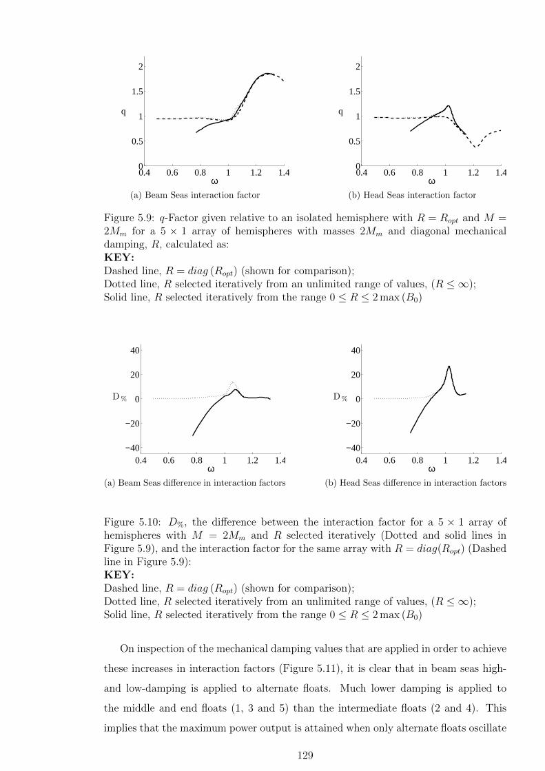
0.4 0.6 0.8 1 1.2 1.40
0.5
1
1.5
2
q
ω(a) Beam Seas interaction factor
0.4 0.6 0.8 1 1.2 1.40
0.5
1
1.5
2
q
ω(b) Head Seas interaction factor
Figure 5.9: q-Factor given relative to an isolated hemisphere with R = Ropt and M =2Mm for a 5 × 1 array of hemispheres with masses 2Mm and diagonal mechanicaldamping, R, calculated as:KEY:Dashed line, R = diag (Ropt) (shown for comparison);Dotted line, R selected iteratively from an unlimited range of values, (R ≤ ∞);Solid line, R selected iteratively from the range 0 ≤ R ≤ 2 max (B0)
0.4 0.6 0.8 1 1.2 1.4−40
−20
0
20
40
D%
ω(a) Beam Seas difference in interaction factors
0.4 0.6 0.8 1 1.2 1.4−40
−20
0
20
40
D%
ω(b) Head Seas difference in interaction factors
Figure 5.10: D%, the difference between the interaction factor for a 5 × 1 array ofhemispheres with M = 2Mm and R selected iteratively (Dotted and solid lines inFigure 5.9), and the interaction factor for the same array with R = diag(Ropt) (Dashedline in Figure 5.9):KEY:Dashed line, R = diag (Ropt) (shown for comparison);Dotted line, R selected iteratively from an unlimited range of values, (R ≤ ∞);Solid line, R selected iteratively from the range 0 ≤ R ≤ 2 max (B0)
On inspection of the mechanical damping values that are applied in order to achieve
these increases in interaction factors (Figure 5.11), it is clear that in beam seas high-
and low-damping is applied to alternate floats. Much lower damping is applied to
the middle and end floats (1, 3 and 5) than the intermediate floats (2 and 4). This
implies that the maximum power output is attained when only alternate floats oscillate
129

and the others remain nearly stationary. Even-numbered floats clearly require large
values of damping (up to 5 max(B0) ) and so the damping on these floats is reduced by
limiting the applied mechanical damping to 2B0 and this reduces the interaction factor
to q = 1.13. In head seas the variation of mechanical damping with float number is
similar to that of Ropt in that damping increases with float number (Ri < Ri+1) for
ks < 0.994 and decreases with float number for ks > 1.07.
0.4 0.6 0.8 1 1.2 1.40
2
4
6
8
10
RB0
ω(a) R ≤ ∞, Beam Seas
0.4 0.6 0.8 1 1.2 1.40
0.5
1
1.5
2
RB0
ω(b) R < 2 max(B0), Beam Seas
0.4 0.6 0.8 1 1.2 1.40
2
4
6
8
10
RB0
ω(c) R ≤ ∞, Head Seas
0.4 0.6 0.8 1 1.2 1.40
0.5
1
1.5
2
RB0
ω(d) R < 2 max(B0), Head Seas
Figure 5.11: Mechanical damping values relative to the maximum radiation dampingon isolated device with R = B and M = 2Mm such that RB0 = R
maxB0chosen in order
to give the maximum Pnet value at each wave frequency for a 5×1 array of hemispheres.KEY:Thick solid black line, float 1 (and 5 in beam seas); Solid grey line, float 2 (and 4 inbeam seas); Dashed line, float 3; Thin solid black line, float 4 (in head seas); Dottedblack line, float 5 (in head seas)
5.5.2 Application to Two-dimensional Rectangular Arrays
5.5.3 5× 2 array, R variation
Applying the same approach to obtain float-specific mechanical damping values for
each float in a 5 x 2 array yields the Q- and q-factors shown in Figures 5.12 and 5.13
respectively. For both array orientations, interaction factors are increased (compared
130
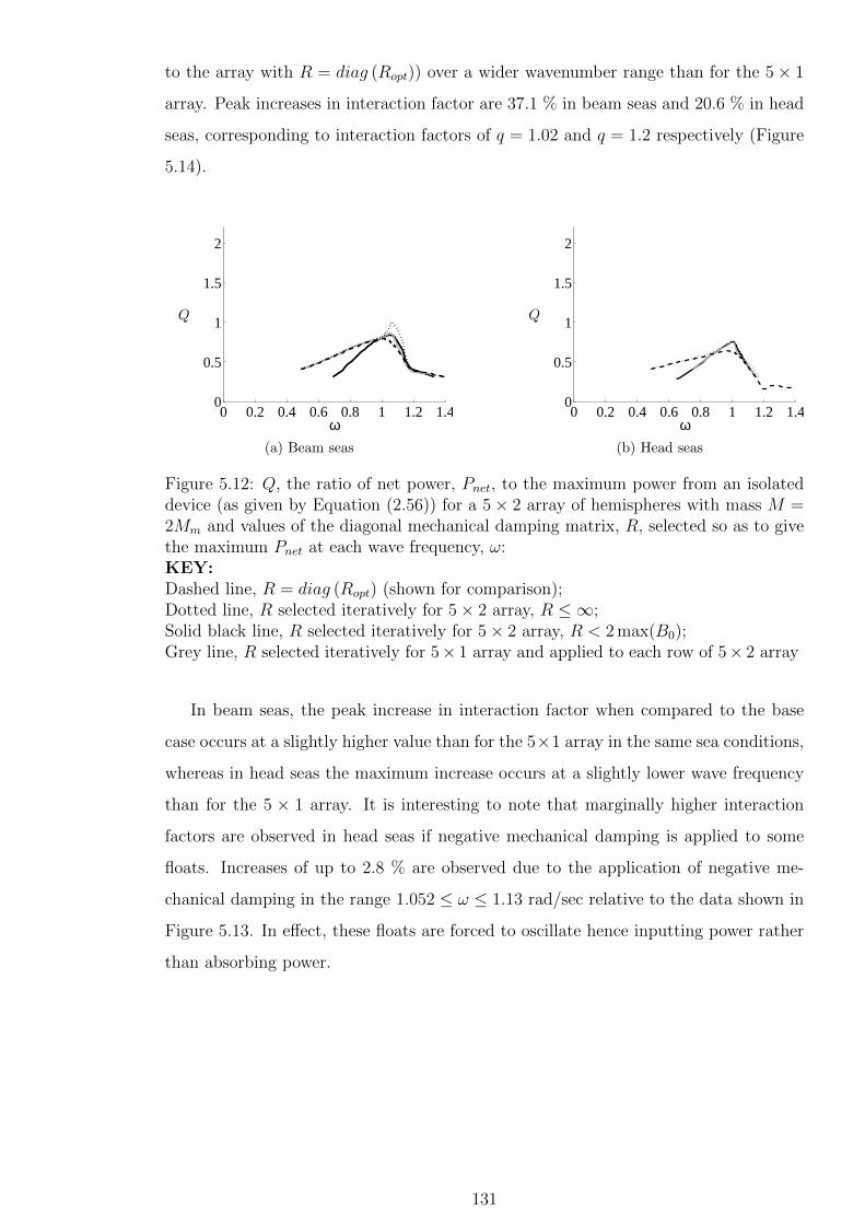
to the array with R = diag (Ropt)) over a wider wavenumber range than for the 5× 1
array. Peak increases in interaction factor are 37.1 % in beam seas and 20.6 % in head
seas, corresponding to interaction factors of q = 1.02 and q = 1.2 respectively (Figure
5.14).
0 0.2 0.4 0.6 0.8 1 1.2 1.40
0.5
1
1.5
2
Q
ω(a) Beam seas
0 0.2 0.4 0.6 0.8 1 1.2 1.40
0.5
1
1.5
2
Q
ω(b) Head seas
Figure 5.12: Q, the ratio of net power, Pnet, to the maximum power from an isolateddevice (as given by Equation (2.56)) for a 5× 2 array of hemispheres with mass M =2Mm and values of the diagonal mechanical damping matrix, R, selected so as to givethe maximum Pnet at each wave frequency, ω:KEY:Dashed line, R = diag (Ropt) (shown for comparison);Dotted line, R selected iteratively for 5× 2 array, R ≤ ∞;Solid black line, R selected iteratively for 5× 2 array, R < 2 max(B0);Grey line, R selected iteratively for 5× 1 array and applied to each row of 5× 2 array
In beam seas, the peak increase in interaction factor when compared to the base
case occurs at a slightly higher value than for the 5×1 array in the same sea conditions,
whereas in head seas the maximum increase occurs at a slightly lower wave frequency
than for the 5 × 1 array. It is interesting to note that marginally higher interaction
factors are observed in head seas if negative mechanical damping is applied to some
floats. Increases of up to 2.8 % are observed due to the application of negative me-
chanical damping in the range 1.052 ≤ ω ≤ 1.13 rad/sec relative to the data shown in
Figure 5.13. In effect, these floats are forced to oscillate hence inputting power rather
than absorbing power.
131
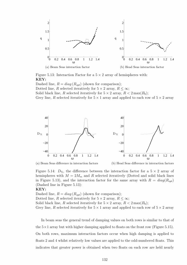
0 0.2 0.4 0.6 0.8 1 1.2 1.40
0.5
1
1.5
2
q
ω(a) Beam Seas interaction factor
0 0.2 0.4 0.6 0.8 1 1.2 1.40
0.5
1
1.5
2
q
ω(b) Head Seas interaction factor
Figure 5.13: Interaction Factor for a 5× 2 array of hemispheres with:KEY:Dashed line, R = diag (Ropt) (shown for comparison);Dotted line, R selected iteratively for 5× 2 array, R ≤ ∞;Solid black line, R selected iteratively for 5× 2 array, R < 2 max(B0);Grey line, R selected iteratively for 5× 1 array and applied to each row of 5× 2 array
0 0.2 0.4 0.6 0.8 1 1.2 1.4−40
−20
0
20
40
D%
ω(a) Beam Seas difference in interaction factors
0 0.2 0.4 0.6 0.8 1 1.2 1.4−40
−20
0
20
40
D%
ω(b) Head Seas difference in interaction factors
Figure 5.14: D%, the difference between the interaction factor for a 5 × 2 array ofhemispheres with M = 2Mm and R selected iteratively (Dotted and solid black linesin Figure 5.13), and the interaction factor for the same array with R = diag(Ropt)(Dashed line in Figure 5.13):KEY:Dashed line, R = diag (Ropt) (shown for comparison);Dotted line, R selected iteratively for 5× 2 array, R ≤ ∞;Solid black line, R selected iteratively for 5× 2 array, R < 2 max(B0);Grey line, R selected iteratively for 5× 1 array and applied to each row of 5× 2 array
In beam seas the general trend of damping values on both rows is similar to that of
the 5×1 array but with higher damping applied to floats on the front row (Figure 5.15).
On both rows, maximum interaction factors occur when high damping is applied to
floats 2 and 4 whilst relatively low values are applied to the odd-numbered floats. This
indicates that greater power is obtained when two floats on each row are held nearly
132
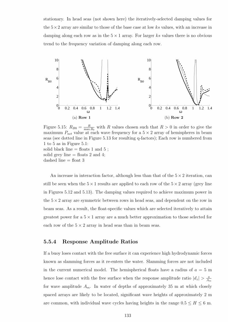
stationary. In head seas (not shown here) the iteratively-selected damping values for
the 5×2 array are similar to those of the base case at low ks values, with an increase in
damping along each row as in the 5× 1 array. For larger ks values there is no obvious
trend to the frequency variation of damping along each row.
0 0.2 0.4 0.6 0.8 1 1.2 1.40
2
4
6
8
10
RB0
ω(a) Row 1
0 0.2 0.4 0.6 0.8 1 1.2 1.40
2
4
6
8
10
RB0
ω(b) Row 2
Figure 5.15: RB0 = RmaxB0
with R values chosen such that R > 0 in order to give themaximum Pnet value at each wave frequency for a 5× 2 array of hemispheres in beamseas (see dotted line in Figure 5.13 for resulting q-factors); Each row is numbered from1 to 5 as in Figure 5.1:solid black line = floats 1 and 5 ;solid grey line = floats 2 and 4;dashed line = float 3
An increase in interaction factor, although less than that of the 5× 2 iteration, can
still be seen when the 5× 1 results are applied to each row of the 5× 2 array (grey line
in Figures 5.12 and 5.13). The damping values required to achieve maximum power in
the 5× 2 array are symmetric between rows in head seas, and dependent on the row in
beam seas. As a result, the float-specific values which are selected iteratively to attain
greatest power for a 5× 1 array are a much better approximation to those selected for
each row of the 5× 2 array in head seas than in beam seas.
5.5.4 Response Amplitude Ratios
If a buoy loses contact with the free surface it can experience high hydrodynamic forces
known as slamming forces as it re-enters the water. Slamming forces are not included
in the current numerical model. The hemispherical floats have a radius of a = 5 m
hence lose contact with the free surface when the response amplitude ratio |dz| > aAm
for wave amplitude Am. In water of depths of approximately 35 m at which closely
spaced arrays are likely to be located, significant wave heights of approximately 2 m
are common, with individual wave cycles having heights in the range 0.5 ≤ H ≤ 6 m.
133

With a wave height of 2 m (hence wave amplitude of Am = 1 m) slamming forces are
likely to occur when |dz| > 5.
The response amplitude ratios corresponding to the arrays with the iteratively-
selected float-specific damping applied can be seen in Figures 5.16 and 5.17, where
response amplitude ratio is the ratio of the absolute response of the float to the wave
amplitude. In all cases, the effect of the large damping values at low and high fre-
quencies is simply achieving a response amplitude of approximately 1 on all floats. In
both incident wave directions of the 5× 1 and 5× 2 array float 3 attains the greatest
response amplitude. In beam seas, the peak in damping on the intermediate floats of
the 5×1 array and the second row of 5×2 array (2,4,7 and 9) in the range of the peak
net power, results in a reduction in response amplitude on these floats.
In the peak net power frequency range there is a reduction in damping applied
to the second row of the 5 × 2 array in beam seas compared to the first row. As
a result, the response amplitudes are much greater on the floats in the second row
compared to the first row, reaching response amplitudes up to 4.6 on float 3. This
means that the absolute response of the float (in m) is 4.6 times the amplitude of
the wave. With such a high response amplitude ratio, slamming forces are likely to
occur when H > 2×(
54.6
)= 2.17 m. This includes all waves close to the approximate
expected significant wave height of Hs = 2 m so is highly probable. The large increase
in interaction factor of 37.1 % with an interaction factor of q = 1.02 compared to the
base case for which q = 0.75 as calculated for the fixed mass 5× 2 array in beam seas
is therefore not necessarily attainable for the specified floats.
The greatest response amplitudes required for the 5× 1 array in beam seas is only
3.2. The neglection of slamming forces in the model is therefore inappropriate when
H > 3.13 m. The large interaction factors (up to q = 1.2) calculated for this array
are consistent with the assumptions made in the calculation method for wave heights
close to the expected significant wave height of 2 m. A similar argument confirms the
validity of the response amplitude ratios for the 5× 2 array in head seas, however this
only results in an interaction factor less than one.
134
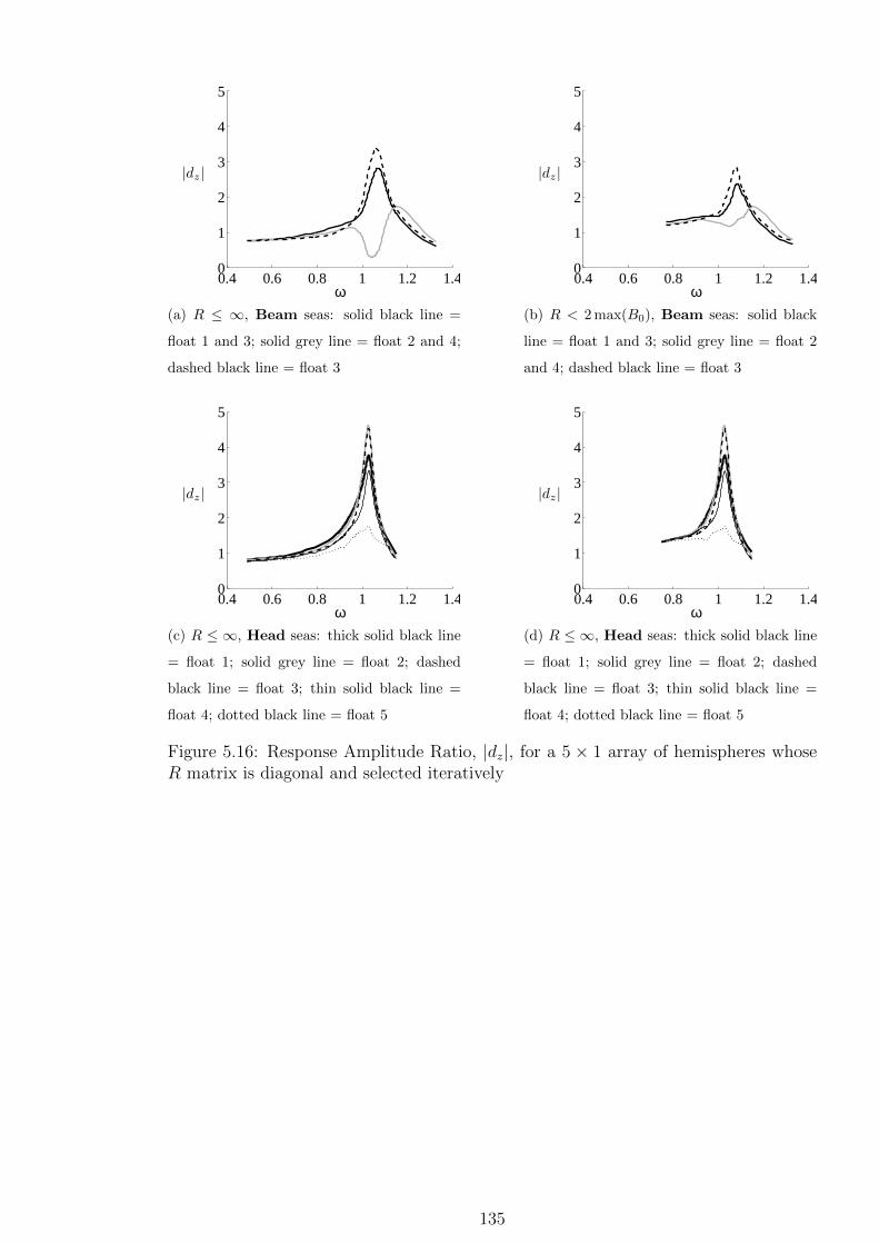
0.4 0.6 0.8 1 1.2 1.40
1
2
3
4
5
|dz|
ω(a) R ≤ ∞, Beam seas: solid black line =
float 1 and 3; solid grey line = float 2 and 4;
dashed black line = float 3
0.4 0.6 0.8 1 1.2 1.40
1
2
3
4
5
|dz|
ω(b) R < 2 max(B0), Beam seas: solid black
line = float 1 and 3; solid grey line = float 2
and 4; dashed black line = float 3
0.4 0.6 0.8 1 1.2 1.40
1
2
3
4
5
|dz|
ω(c) R ≤ ∞, Head seas: thick solid black line
= float 1; solid grey line = float 2; dashed
black line = float 3; thin solid black line =
float 4; dotted black line = float 5
0.4 0.6 0.8 1 1.2 1.40
1
2
3
4
5
|dz|
ω(d) R ≤ ∞, Head seas: thick solid black line
= float 1; solid grey line = float 2; dashed
black line = float 3; thin solid black line =
float 4; dotted black line = float 5
Figure 5.16: Response Amplitude Ratio, |dz|, for a 5 × 1 array of hemispheres whoseR matrix is diagonal and selected iteratively
135
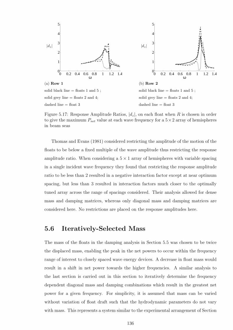
0 0.2 0.4 0.6 0.8 1 1.2 1.40
1
2
3
4
5
|dz|
ω(a) Row 1
solid black line = floats 1 and 5 ;
solid grey line = floats 2 and 4;
dashed line = float 3
0 0.2 0.4 0.6 0.8 1 1.2 1.40
1
2
3
4
5
|dz|
ω(b) Row 2
solid black line = floats 1 and 5 ;
solid grey line = floats 2 and 4;
dashed line = float 3
Figure 5.17: Response Amplitude Ratios, |dz|, on each float when R is chosen in orderto give the maximum Pnet value at each wave frequency for a 5×2 array of hemispheresin beam seas
Thomas and Evans (1981) considered restricting the amplitude of the motion of the
floats to be below a fixed multiple of the wave amplitude thus restricting the response
amplitude ratio. When considering a 5× 1 array of hemispheres with variable spacing
in a single incident wave frequency they found that restricting the response amplitude
ratio to be less than 2 resulted in a negative interaction factor except at near optimum
spacing, but less than 3 resulted in interaction factors much closer to the optimally
tuned array across the range of spacings considered. Their analysis allowed for dense
mass and damping matrices, whereas only diagonal mass and damping matrices are
considered here. No restrictions are placed on the response amplitudes here.
5.6 Iteratively-Selected Mass
The mass of the floats in the damping analysis in Section 5.5 was chosen to be twice
the displaced mass, enabling the peak in the net powers to occur within the frequency
range of interest to closely spaced wave energy devices. A decrease in float mass would
result in a shift in net power towards the higher frequencies. A similar analysis to
the last section is carried out in this section to iteratively determine the frequency
dependent diagonal mass and damping combinations which result in the greatest net
power for a given frequency. For simplicity, it is assumed that mass can be varied
without variation of float draft such that the hydrodynamic parameters do not vary
with mass. This represents a system similar to the experimental arrangement of Section
136
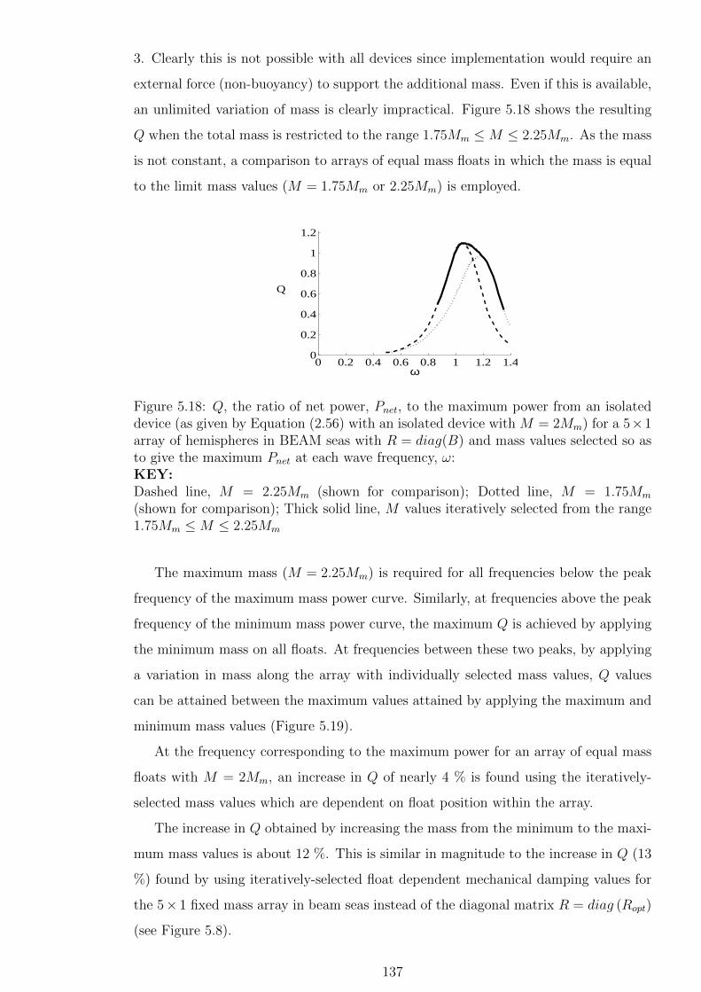
3. Clearly this is not possible with all devices since implementation would require an
external force (non-buoyancy) to support the additional mass. Even if this is available,
an unlimited variation of mass is clearly impractical. Figure 5.18 shows the resulting
Q when the total mass is restricted to the range 1.75Mm ≤M ≤ 2.25Mm. As the mass
is not constant, a comparison to arrays of equal mass floats in which the mass is equal
to the limit mass values (M = 1.75Mm or 2.25Mm) is employed.
0 0.2 0.4 0.6 0.8 1 1.2 1.40
0.2
0.4
0.6
0.8
1
1.2
Q
ω
Figure 5.18: Q, the ratio of net power, Pnet, to the maximum power from an isolateddevice (as given by Equation (2.56) with an isolated device with M = 2Mm) for a 5×1array of hemispheres in BEAM seas with R = diag(B) and mass values selected so asto give the maximum Pnet at each wave frequency, ω:KEY:Dashed line, M = 2.25Mm (shown for comparison); Dotted line, M = 1.75Mm
(shown for comparison); Thick solid line, M values iteratively selected from the range1.75Mm ≤M ≤ 2.25Mm
The maximum mass (M = 2.25Mm) is required for all frequencies below the peak
frequency of the maximum mass power curve. Similarly, at frequencies above the peak
frequency of the minimum mass power curve, the maximum Q is achieved by applying
the minimum mass on all floats. At frequencies between these two peaks, by applying
a variation in mass along the array with individually selected mass values, Q values
can be attained between the maximum values attained by applying the maximum and
minimum mass values (Figure 5.19).
At the frequency corresponding to the maximum power for an array of equal mass
floats with M = 2Mm, an increase in Q of nearly 4 % is found using the iteratively-
selected mass values which are dependent on float position within the array.
The increase in Q obtained by increasing the mass from the minimum to the maxi-
mum mass values is about 12 %. This is similar in magnitude to the increase in Q (13
%) found by using iteratively-selected float dependent mechanical damping values for
the 5× 1 fixed mass array in beam seas instead of the diagonal matrix R = diag (Ropt)
(see Figure 5.8).
137
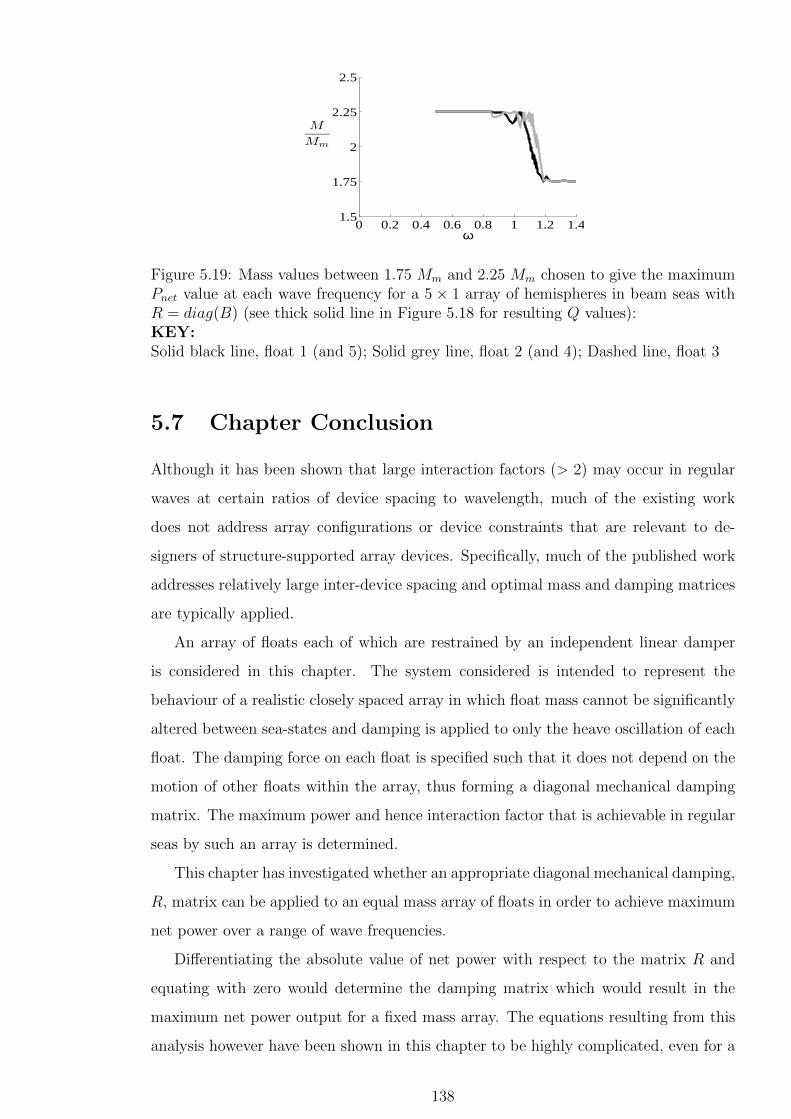
0 0.2 0.4 0.6 0.8 1 1.2 1.41.5
1.75
2
2.25
2.5
M
Mm
ω
Figure 5.19: Mass values between 1.75 Mm and 2.25 Mm chosen to give the maximumPnet value at each wave frequency for a 5× 1 array of hemispheres in beam seas withR = diag(B) (see thick solid line in Figure 5.18 for resulting Q values):KEY:Solid black line, float 1 (and 5); Solid grey line, float 2 (and 4); Dashed line, float 3
5.7 Chapter Conclusion
Although it has been shown that large interaction factors (> 2) may occur in regular
waves at certain ratios of device spacing to wavelength, much of the existing work
does not address array configurations or device constraints that are relevant to de-
signers of structure-supported array devices. Specifically, much of the published work
addresses relatively large inter-device spacing and optimal mass and damping matrices
are typically applied.
An array of floats each of which are restrained by an independent linear damper
is considered in this chapter. The system considered is intended to represent the
behaviour of a realistic closely spaced array in which float mass cannot be significantly
altered between sea-states and damping is applied to only the heave oscillation of each
float. The damping force on each float is specified such that it does not depend on the
motion of other floats within the array, thus forming a diagonal mechanical damping
matrix. The maximum power and hence interaction factor that is achievable in regular
seas by such an array is determined.
This chapter has investigated whether an appropriate diagonal mechanical damping,
R, matrix can be applied to an equal mass array of floats in order to achieve maximum
net power over a range of wave frequencies.
Differentiating the absolute value of net power with respect to the matrix R and
equating with zero would determine the damping matrix which would result in the
maximum net power output for a fixed mass array. The equations resulting from this
analysis however have been shown in this chapter to be highly complicated, even for a
138

basic two element array.
Three approaches for obtaining a diagonal damping matrix have instead been con-
sidered based on i) the radiation damping matrix, ii) the optimal damping equation
for an isolated device and iii) an iterative approach. For a particular frequency, the
values of mechanical damping required on each float within the array that maximise
net power output do not appear to be directly related to the diagonal elements of the
radiation damping matrix (R = diag(B)).
Over most of the frequency range, the diagonal of the optimal damping matrix for a
fixed mass system provides maximum net power. In this case there is minimal difference
between the damping of each float. However, close to the maximum power output from
an isolated device, greater net power can be obtained by using damping values that
are determined by an iterative approach. Here a Levenberg-Marquardt algorithm is
employed for the iteration, however other methods could be used. For a 5 × 1 array
of hemispherical floats, application of a diagonal damping matrix whose elements are
selected iteratively is found to increase the net power by up to 12 % in beam seas and
18 % in head seas compared to when the diagonal elements of the damping matrix are
selected according to the optimal damping equation for an isolated device. When a
restriction, R ≤ 2 maxB0, is placed on the range of R values permitted in the iterative
procedure, the peak increase reduces to ∼ 7 % in beam seas.
The interaction factors for an array with an optimal (dense) mechanical damping
matrix differ considerably from those for an array with individual mechanical damping
on each float (diagonal damping matrix).
For the array in beam seas, increased power output only occurs when alternate
floats are nearly stationary and, if this is not possible, power output is similar to that
obtained by applying mechanical damping similar to the hydrodynamic damping of
each float. In head seas, maximum power output is obtained at low wavenumbers if
mechanical damping is increased with row number. In contrast, at high wavenumbers,
net power output is maximum when damping is greatest on the front float.
The optimal damping values iteratively selected to achieve maximum power in a
5×2 array are symmetric between rows in head seas, and dependent on the row in beam
seas. Peak increases in interaction factor (compared to when the diagonal elements of
the damping matrix are selected according to the optimal damping equation for an
isolated device) are 37.1 % in beam seas and 20.6 % in head seas for the 5 × 2 array.
These increases correspond to interaction factors of q = 1.02 and q = 1.2 in beam and
head seas respectively. An increase in interaction factor, although less than that of the
139

5× 2 iteration, can be seen when the 5× 1 results are applied to each row of the 5× 2
array. The application of these 5 × 1 values to each row of the 5 × 2 array is a much
closer approximation to the values actually selected to achieve the greatest power for
the 5× 2 array in head seas than in beam seas.
A similar iterative approach has also been used to determine a unique mass for each
float in order to maximise net power. A system by which both the mass and the damp-
ing could be varied within limited ranges would allow for even greater manipulation
of the power output. Using the current method to determine such M and R values
however would require numerous iterations, and would be computationally inefficient.
At the frequency corresponding to the maximum power for an array of equal mass
floats with M = 2Mm, an increase in Q of nearly 4 % is found using the iteratively-
selected mass values which are dependent on float position within the array. Assuming
mechanical damping to be equal to the diagonal of the radiation damping matrix, sim-
ilar increases of net power are found if the mass of each float is varied from 1.75Mm to
2.25Mm on all floats as the increase found by using iteratively-selected float dependent
mechanical damping values for the 5× 1 fixed mass array in beam seas instead of the
diagonal matrix R = diag (Ropt).
140

Chapter 6
Optimisation of Geometries
Mechanical damping values have been determined in Chapter 5 which could be applied
directly to each float within a linear array with fixed geometries and spacing in order
to achieve the greatest power. In some cases impractically high values of mechani-
cal damping were deemed necessary. As the radiation damping is dependent on the
submerged geometry, the total damping (consisting of the radiation and mechanical
damping) could also be varied by varying the submerged geometries of the floats within
the array, thus reducing the amount of mechanical damping required to achieve the
maximum power (at a given frequency).
This chapter considers the possibility that a reduction in required mechanical damp-
ing could be achieved by using alternative float geometries without reducing the net
power from the array. It is assumed that the hydrodynamic parameters are known for
all geometries considered. A method to select the most appropriate geometry from
a selection of geometries is required. The calculation of power requires a mechanical
damping force to be applied. As the range of geometries considered could be large,
and the range of possible mechanical values infinite, the method to select geometries
must not depend on the calculation of power for each possible geometry.
Two geometry selection criteria are considered for a range of geometries. The
first considers only the magnitude of radiation damping on each float with a view to
achieving a specific (optimal) magnitude of total damping. As well as the radiation
damping, the added mass, excitation force and in some cases the hydrostatic stiffness
and float mass are all dependent on the submerged float geometry. For certain groups of
geometries, the variation of all of these hydrodynamic parameters is significant, hence
must be accounted for when selecting a geometry. The free-float response amplitude
ratio is therefore considered as a second selection criterion as it incorporates all of these
hydrodynamic parameters but not mechanical damping.
141
The geometry selection criterion which accounts only for the variation in radiation
damping would require the variation in all other hydrodynamic parameters with geom-
etry to be minimal. The geometry which would require the least mechanical damping
to achieve a specific total (radiation plus mechanical) damping would be selected. The
desired total damping would be determined for a specific base geometry using the it-
erative method described in Chapter 5. For free-float response to be an appropriate
measure there must be a correlation between the geometries which achieve the greatest
free-float response and those which achieve the greatest power under the application
of a mechanical damping force.
To select the most suitable geometry for each position within an array, knowledge of
the interaction of that float geometry with all of the other float geometries is required.
If the size of the array is large, then this would require knowledge of many combinations
of the floats in order to select the most appropriate float geometry for each position
within an array. Section 6.1 presents an argument for using only the knowledge of the
interaction of each float with the float directly adjacent to it within a large linear array
to determine the most appropriate geometry for each position within the array.
Whilst several independent geometries are considered, it is recognised that simply
varying the draft of a float of fixed overall geometry results in a variation in submerged
geometry, hence allows for the manipulation of hydrodynamic parameters according
to the current wave conditions. An investigation into the use of both radiation damp-
ing and free-float response amplitude ratio as draft selection methods is presented in
Section 6.2 for several geometries placed in isolation.
A method to select the most appropriate draft to operate over a range of wave
frequencies is considered in Section 6.3 and applied to a specific complex geometry,
ConTop.
Section 6.4 considers a small array of basic and equal geometry floats for which
the optimal diagonal mechanical damping matrix (determined using the optimisation
procedure of Chapter 5) is known. Based on the findings of the isolated device in Section
6.2, an appropriate method is used to determine at which frequencies the mechanical
damping could be reduced by varying the draft of the floats (equally) without reducing
the total power from the array.
142
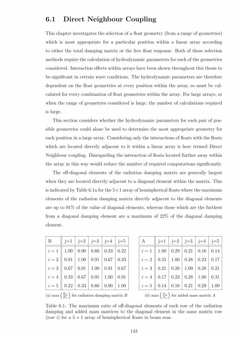
6.1 Direct Neighbour Coupling
This chapter investigates the selection of a float geometry (from a range of geometries)
which is most appropriate for a particular position within a linear array according
to either the total damping matrix or the free float response. Both of these selection
methods require the calculation of hydrodynamic parameters for each of the geometries
considered. Interaction effects within arrays have been shown throughout this thesis to
be significant in certain wave conditions. The hydrodynamic parameters are therefore
dependent on the float geometries at every position within the array, so must be cal-
culated for every combination of float geometries within the array. For large arrays, or
when the range of geometries considered is large, the number of calculations required
is large.
This section considers whether the hydrodynamic parameters for each pair of pos-
sible geometries could alone be used to determine the most appropriate geometry for
each position in a large array. Considering only the interactions of floats with the floats
which are located directly adjacent to it within a linear array is here termed Direct
Neighbour coupling. Disregarding the interaction of floats located further away within
the array in this way would reduce the number of required computations significantly.
The off-diagonal elements of the radiation damping matrix are generally largest
when they are located directly adjacent to a diagonal element within the matrix. This
is indicated by Table 6.1a for the 5×1 array of hemispherical floats where the maximum
elements of the radiation damping matrix directly adjacent to the diagonal elements
are up to 91% of the value of diagonal elements, whereas those which are the furthest
from a diagonal damping element are a maximum of 22% of the diagonal damping
element.
B j=1 j=2 j=3 j=4 j=5
i = 1 1.00 0.90 0.66 0.33 0.22
i = 2 0.91 1.00 0.91 0.67 0.33
i = 3 0.67 0.91 1.00 0.91 0.67
i = 4 0.33 0.67 0.91 1.00 0.91
i = 5 0.22 0.33 0.66 0.90 1.00
(a) max(
Bij
Bii
)for radiation damping matrix B
A j=1 j=2 j=3 j=4 j=5
i = 1 1.00 0.29 0.21 0.16 0.14
i = 2 0.31 1.00 0.28 0.23 0.17
i = 3 0.21 0.28 1.00 0.28 0.21
i = 4 0.17 0.23 0.28 1.00 0.31
i = 5 0.14 0.16 0.21 0.29 1.00
(b) max(
Aij
Aii
)for added mass matrix A
Table 6.1: The maximum ratio of off-diagonal elements of each row of the radiationdamping and added mass matrices to the diagonal element in the same matrix row(row i) for a 5× 1 array of hemispherical floats in beam seas
143
This suggests that float geometries within an array could be selected based on only
the coupling between directly adjacent floats. This would require knowledge of the
hydrodynamic parameters corresponding to each combination of two geometries from
a discrete range regardless of the overall size of the array.
The ratio between the off-diagonal and diagonal added mass elements is generally
smaller than that of the radiation damping matrix, with the off diagonal elements
corresponding to between 14 % and 31 % of the diagonal elements for the 5×1 array of
hemispherical floats in beam seas. As with the radiation damping matrix, Table 6.1b
indicates that this is focused mainly on the elements directly adjacent to the diagonal
elements, supporting the argument for the use of Direct-Neighbour Coupling.
6.2 Draft Variation of Isolated Body
Before the direct coupling of different geometry floats is considered, it is useful to obtain
an understanding of the effect of the variation of draft of isolated floats. The magnitude
of variation of radiation damping with float geometry compared to the magnitude of
variation of other hydrodynamic parameters should give an indication of whether the
radiation damping can be used as an indicator of which draft is most appropriate (where
knowledge of the optimal total damping is known). A correlation between the free-
float response and the maximum power under the application of different mechanical
damping values would indicate the free-float response amplitude ratio as an effective
selection criterion.
The free-float Response Amplitude Ratio of the floats (given by Equation (3.3))
combines the added mass, radiation damping and excitation force together with hy-
drostatic stiffness, which is independent of draft of the vertical circular cylinder, and
the float mass. The objective is to understand the relationship between free float
response amplitude |za| and the power output of the same float P when subject to me-
chanical damping, R. To do this comparison it is necessary to a) understand variation
of hydrodynamic parameters with draft, b) specify mass (two types considered) and c)
calculate response and power (as per figure 6.4).
The hydrostatic stiffness is dependent on the cross-sectional area of the float at the
water plane (see Section 3). A draft variation for a float for which the water-plane area
remains constant allows for a variation in submerged float geometry without varying
the hydrostatic stiffness, thus reducing the parameters to consider.
Three float geometries are considered in this section at different depths (see Figure
144
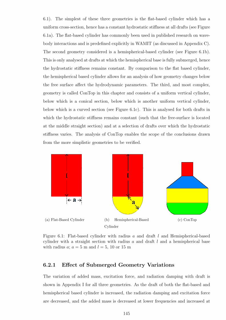
6.1). The simplest of these three geometries is the flat-based cylinder which has a
uniform cross-section, hence has a constant hydrostatic stiffness at all drafts (see Figure
6.1a). The flat-based cylinder has commonly been used in published research on wave-
body interactions and is predefined explicitly in WAMIT (as discussed in Appendix C).
The second geometry considered is a hemispherical-based cylinder (see Figure 6.1b).
This is only analysed at drafts at which the hemispherical base is fully submerged, hence
the hydrostatic stiffness remains constant. By comparison to the flat based cylinder,
the hemispherical based cylinder allows for an analysis of how geometry changes below
the free surface affect the hydrodynamic parameters. The third, and most complex,
geometry is called ConTop in this chapter and consists of a uniform vertical cylinder,
below which is a conical section, below which is another uniform vertical cylinder,
below which is a curved section (see Figure 6.1c). This is analysed for both drafts in
which the hydrostatic stiffness remains constant (such that the free-surface is located
at the middle straight section) and at a selection of drafts over which the hydrostatic
stiffness varies. The analysis of ConTop enables the scope of the conclusions drawn
from the more simplistic geometries to be verified.
(a) Flat-Based Cylinder (b) Hemispherical-Based
Cylinder
(c) ConTop
Figure 6.1: Flat-based cylinder with radius a and draft l and Hemispherical-basedcylinder with a straight section with radius a and draft l and a hemispherical basewith radius a; a = 5 m and l = 5, 10 or 15 m
6.2.1 Effect of Submerged Geometry Variations
The variation of added mass, excitation force, and radiation damping with draft is
shown in Appendix I for all three geometries. As the draft of both the flat-based and
hemispherical based cylinder is increased, the radiation damping and excitation force
are decreased, and the added mass is decreased at lower frequencies and increased at
145

higher frequencies.
0 0.2 0.4 0.6 0.8 1 1.2 1.430
32
34
36
38
40
ω
A−%
(a) Added Mass: A−% = 100− 100 |Ah||Af |
0 0.2 0.4 0.6 0.8 1 1.2 1.40
10
20
30
40
50
60
ω
B−%
(b) Radiation Damping: B−% = 100−100 |Bh||Bf |
0 0.2 0.4 0.6 0.8 1 1.2 1.40
5
10
15
20
25
30
35
ω
F−%
(c) Excitation Force: F−% = 100− 100 |Fh||Ff |
Figure 6.2: Percentage reduction in hydrodynamic parameters from the flat basedcylinder of radius a = 5 m and draft l (see Figures 6.1a and I.1) to the hemispherical-based cylinder of radius a and straight section length l (see Figures 6.1b and I.2); Af ,Bf and Ff are the flat-based cylinder’s added mass, radiation damping and excitationforce respectively, and Ah, Bh and Fh are the hemispherical-based cylinder’s addedmass, radiation damping and excitation force respectively:KEY:Solid black line, l = 3a; Grey line, l = 2a; Dashed black line, l = a
Comparison of the hydrodynamic parameters at different drafts for the flat and
hemispherical based cylinders with equal length straight sections is shown in Figure
6.2. The effect of including a hemispherical base to the straight cylinder is to decrease
the added mass by 35 to 40% at all frequencies and decrease the radiation damping
and excitation force with increasing frequency with a maximum decrease of 57 % and
35 % respectively at high wave frequencies. The decrease in all three hydrodynamic
parameters due to the inclusion of the hemispherical base is more significant for the
shallower draft floats (such that the dashed line is greater than the grey and black
soild lines in figure 6.2) over the majority of the frequency range. This indicates that
geometry variations close to the free surface are of greatest importance in float designs.
146

6.2.2 Radiation Damping as a Geometry Selection Criterion
The radiation damping is the parameter which varies the greatest between drafts for
both the flat based and hemispherically based cylinders (see Appendix Sections I.1.1
and I.1.2). Similarly, changes of ConTop draft for which the free surface remains at
the middle vertical straight edge of the geometry results in only minor variations in
added mass and excitation force compared to large variations in radiation damping
(see Appendix I.1.3). This indicates that selecting drafts based on the damping alone
could be sufficient to select the most appropriate float draft from a range of drafts with
constant hydrostatic stiffness.
The added mass, excitation force and radiation damping all vary considerably how-
ever between drafts of ConTop which have different hydrostatic stiffness values (see
Appendix I.1.3). Selecting drafts from a selection of drafts in which the water-plane
area varies therefore requires a more complex criteria than the radiation damping alone.
6.2.3 |dz|R=0 as a Geometry Selection Criterion
Although less than the radiation damping in some cases, the added mass and exci-
tation force do vary with draft so a measure which accounts for the variation in all
three parameters would be preferable. The free-float response amplitude ratio (|dz|R=0)
connects all three parameters (Equation (3.1) with R = 0), however in order for power
to be absorbed a mechanical damping force must be applied, thus varying the float
response. This section determines whether free-float response can be used as an in-
dicator of which float draft will absorb the most power over a given frequency range
when different values of mechanical damping are applied.
Three sets of geometries are considered. The first set consists of three drafts of
flat based cylinder with l = 5 m, 10 m and 15 m; the second set consists of 6 drafts
of ConTop for which the free-surface is located along the middle uniform cylindrical
section, hence the water-plane area and hydrostatic stiffness remain constant; and the
third set consists of 6 drafts of ConTop over which the hydrostatic stiffness is varied.
Both the |dz|R=0 and power require the mass of the floats to be specified. Two
different mass cases are considered within each geometry set such that the floats are
neutrally buoyant with a draft dependent mass equal to the displaced mass (M = Mm)
or have a constant mass which is independent of draft. The constant masses considered
are equal to the displaced mass of each the drafts within the set.
The power further requires that a mechanical damping value be specified. Two cases
147
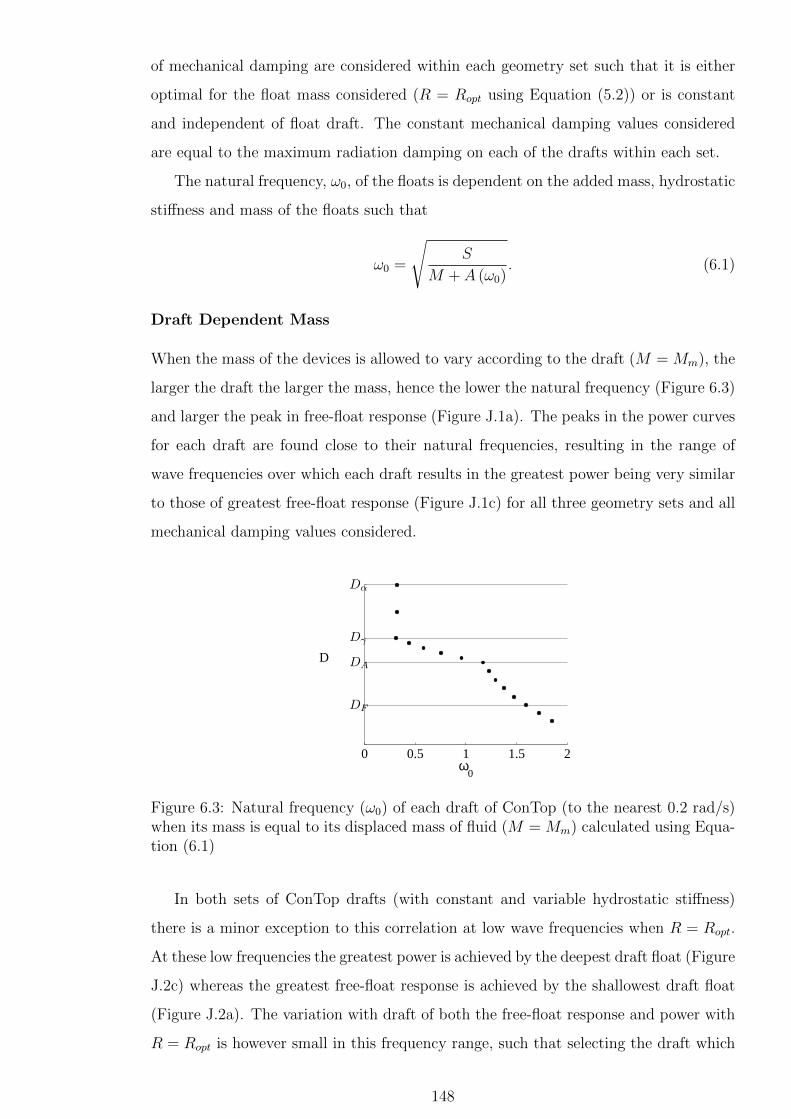
of mechanical damping are considered within each geometry set such that it is either
optimal for the float mass considered (R = Ropt using Equation (5.2)) or is constant
and independent of float draft. The constant mechanical damping values considered
are equal to the maximum radiation damping on each of the drafts within each set.
The natural frequency, ω0, of the floats is dependent on the added mass, hydrostatic
stiffness and mass of the floats such that
ω0 =
√S
M + A (ω0). (6.1)
Draft Dependent Mass
When the mass of the devices is allowed to vary according to the draft (M = Mm), the
larger the draft the larger the mass, hence the lower the natural frequency (Figure 6.3)
and larger the peak in free-float response (Figure J.1a). The peaks in the power curves
for each draft are found close to their natural frequencies, resulting in the range of
wave frequencies over which each draft results in the greatest power being very similar
to those of greatest free-float response (Figure J.1c) for all three geometry sets and all
mechanical damping values considered.
0 0.5 1 1.5 2ω
0
D
DF
DA
Dγ
Dα
Figure 6.3: Natural frequency (ω0) of each draft of ConTop (to the nearest 0.2 rad/s)when its mass is equal to its displaced mass of fluid (M = Mm) calculated using Equa-tion (6.1)
In both sets of ConTop drafts (with constant and variable hydrostatic stiffness)
there is a minor exception to this correlation at low wave frequencies when R = Ropt.
At these low frequencies the greatest power is achieved by the deepest draft float (Figure
J.2c) whereas the greatest free-float response is achieved by the shallowest draft float
(Figure J.2a). The variation with draft of both the free-float response and power with
R = Ropt is however small in this frequency range, such that selecting the draft which
148

achieves the greatest free-float response (the shallowest draft) would result in only a
small decrease in power compared to the deepest draft float.
In the set of ConTop drafts with varying stiffness, an extremely large peak in free-
float response is calculated at a low wave frequency for the draft for which the free
surface is located at the upper-inclined surface (Figure J.3a). This peak does not,
however, translate to a large power output for any mechanical damping value (Figure
J.3c). This extreme peak could be due to motion trapped modes which are coupled
oscillations of the body and the fluid which would not decrease with time in the absence
of viscosity (McIver and McIver, 2007). The extreme peak is predicted as a result of
the limited radiation damping calculated close to the natural frequency. In practice,
the extreme peak would not occur however due to the additional forces which would
be present for these drafts due to sloshing, wave breaking and viscous effects which are
not included within the linear model (Stallard et al., 2009b).
Constant Mass and Constant Stiffness
For the two geometry sets over which the hydrostatic stiffness is constant, when all
drafts within the set have the same mass the natural frequencies are very similar, dif-
fering only due to the slight difference in added mass. For both sets of drafts, the
shallowest draft float achieves the greatest free-float response amplitude ratio for fre-
quencies away from the natural frequency, with different geometries achieving greatest
power close to the natural frequency (Figures J.1b and J.2b).
For the flat based cylindrical drafts, the free float response of the constant mass
floats decreases as the draft increases at low and high frequencies but increases with
increasing draft near the peaks. Small variations in natural frequency can be seen
when the constant mass is small. This is because a small mass corresponds to a high
natural frequency, which is where the variation of added mass with draft is greatest
(see Figure I.1a). The variation in free-float response with draft close to the peaks does
not correspond to the power achieved. The shallowest draft float absorbs the greatest
power over the entire frequency range when the mechanical damping is constant and
over most of the frequency range when the mechanical damping is optimal such that
R = Ropt (figure J.1d).
For the ConTop drafts of constant mass and stiffness, the shallowest draft float
also achieves greatest power when the mechanical damping is constant and large or is
optimal (Figure J.2d). When the mechanical damping is small however, there is no
obvious method to select the float draft which will result in the greatest power. A
149
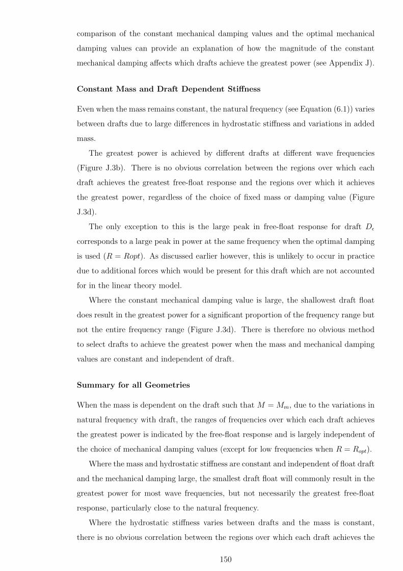
comparison of the constant mechanical damping values and the optimal mechanical
damping values can provide an explanation of how the magnitude of the constant
mechanical damping affects which drafts achieve the greatest power (see Appendix J).
Constant Mass and Draft Dependent Stiffness
Even when the mass remains constant, the natural frequency (see Equation (6.1)) varies
between drafts due to large differences in hydrostatic stiffness and variations in added
mass.
The greatest power is achieved by different drafts at different wave frequencies
(Figure J.3b). There is no obvious correlation between the regions over which each
draft achieves the greatest free-float response and the regions over which it achieves
the greatest power, regardless of the choice of fixed mass or damping value (Figure
J.3d).
The only exception to this is the large peak in free-float response for draft Dε
corresponds to a large peak in power at the same frequency when the optimal damping
is used (R = Ropt). As discussed earlier however, this is unlikely to occur in practice
due to additional forces which would be present for this draft which are not accounted
for in the linear theory model.
Where the constant mechanical damping value is large, the shallowest draft float
does result in the greatest power for a significant proportion of the frequency range but
not the entire frequency range (Figure J.3d). There is therefore no obvious method
to select drafts to achieve the greatest power when the mass and mechanical damping
values are constant and independent of draft.
Summary for all Geometries
When the mass is dependent on the draft such that M = Mm, due to the variations in
natural frequency with draft, the ranges of frequencies over which each draft achieves
the greatest power is indicated by the free-float response and is largely independent of
the choice of mechanical damping values (except for low frequencies when R = Ropt).
Where the mass and hydrostatic stiffness are constant and independent of float draft
and the mechanical damping large, the smallest draft float will commonly result in the
greatest power for most wave frequencies, but not necessarily the greatest free-float
response, particularly close to the natural frequency.
Where the hydrostatic stiffness varies between drafts and the mass is constant,
there is no obvious correlation between the regions over which each draft achieves the
150

greatest free-float response and the regions over which it achieves the greatest power
6.3 Optimal Draft: ConTop
The ConTop geometry (defined in Appendix H) allows for a large variation in power
with small variations in mass hence draft. It was shown in Section 6.2.2 that the
radiation damping alone does not provide a sufficient criterion by which drafts should
be selected to achieve greatest power, where the range of drafts considered involves
variations in the water-plane area hence stiffness. Further to this it was shown in
Section 6.2.3, that the free-float response is also not a sufficient draft selection procedure
where the hydrostatic stiffness varies between drafts but the mass does not.
Where the ConTop float is neutrally buoyant at each draft however, it was demon-
strated in Section 6.2.3 that the draft which results in the greatest power at a particular
wave frequency can be determined from the free-float response, |dz|R=0, without prior
knowledge of the magnitude of mechanical damping. The only exception to this is
at frequencies where the variation in |dz|R=0 between drafts is negligible, however the
variation in power at these frequencies is also negligible.
Sections 6.2.2 and 6.2.3 focused on methods to select drafts so as to achieve greatest
power when an unknown quantity of mechanical damping is applied. In contrast, this
section considers the selection of draft to achieve greatest power when the power which
would be achieved by each draft at each wave frequency is known. In practice, it is
likely that the device will be subjected to a range of frequencies in a short period of
time. Varying the draft of the float to match every wave is not practical. The ideal
selection procedure should allow for the greatest power capture from a device over a
likely range of wave frequencies.
When the mechanical damping is optimal (R = Ropt) and the floats are neutrally
buoyant, large variations in float draft from one frequency to the next are required
to achieve the greatest power at each wave frequency (Figures 6.4a and 6.4b). When
R = Ropt and the mass is constant however, large variations in the selected float drafts
are seen at higher frequencies, even though the difference in power due to the draft
variation is minimal (Figures 6.4c and 6.4d).
151
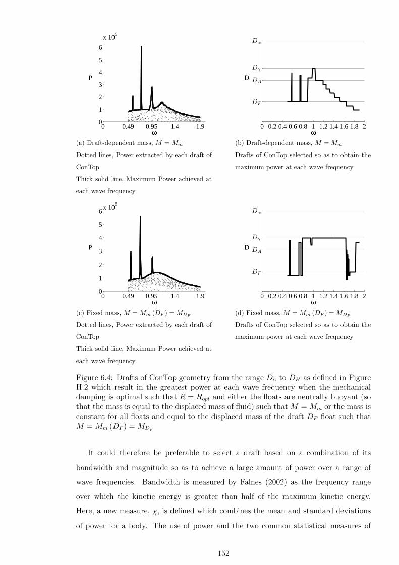
0 0.49 0.95 1.4 1.90
1
2
3
4
5
6
x 105
ω
P
(a) Draft-dependent mass, M = Mm
Dotted lines, Power extracted by each draft of
ConTop
Thick solid line, Maximum Power achieved at
each wave frequency
0 0.2 0.4 0.6 0.8 1 1.2 1.4 1.6 1.8 2ω
D
DF
DA
Dγ
Dα
(b) Draft-dependent mass, M = Mm
Drafts of ConTop selected so as to obtain the
maximum power at each wave frequency
0 0.49 0.95 1.4 1.90
1
2
3
4
5
6x 10
5
ω
P
(c) Fixed mass, M = Mm (DF ) = MDF
Dotted lines, Power extracted by each draft of
ConTop
Thick solid line, Maximum Power achieved at
each wave frequency
0 0.2 0.4 0.6 0.8 1 1.2 1.4 1.6 1.8 2ω
D
DF
DA
Dγ
Dα
(d) Fixed mass, M = Mm (DF ) = MDF
Drafts of ConTop selected so as to obtain the
maximum power at each wave frequency
Figure 6.4: Drafts of ConTop geometry from the range Dα to DH as defined in FigureH.2 which result in the greatest power at each wave frequency when the mechanicaldamping is optimal such that R = Ropt and either the floats are neutrally buoyant (sothat the mass is equal to the displaced mass of fluid) such that M = Mm or the mass isconstant for all floats and equal to the displaced mass of the draft DF float such thatM = Mm (DF ) = MDF
It could therefore be preferable to select a draft based on a combination of its
bandwidth and magnitude so as to achieve a large amount of power over a range of
wave frequencies. Bandwidth is measured by Falnes (2002) as the frequency range
over which the kinetic energy is greater than half of the maximum kinetic energy.
Here, a new measure, χ, is defined which combines the mean and standard deviations
of power for a body. The use of power and the two common statistical measures of
152
mean and standard deviation is used instead here to follow on more fluently from other
common measures in the industry such as the interaction factor. The most suitable
float geometry to absorb power for a range of frequencies will have the lowest value of
χ where χ is defined to be
χ(l) = P × Std(P ), (6.2)
where P is the mean power across the frequency range, and Std(P ) is the standard
deviation of power over the range of frequencies.
Figure 6.5 shows the results of using χ to select ConTop drafts for three different
frequency ranges. Whilst the drafts selected to maximise χ do not give the greatest
power at all frequencies within the range, they do achieve a large and consistent amount
of power which could be preferable when frequencies are expected to vary within a
certain range. In particular, there is very little reduction in power in the range 1.4 ≤ω ≤ 1.9 rad/sec as a result of using draft Dδ which is selected by χ (Figures 6.5c and
6.5d) instead of using the large range of drafts (from DH to Dγ) which give the greatest
power at different frequencies within this frequency range (Figures 6.4c and 6.4d).
153

0 0.49 0.95 1.4 1.90
1
2
3
4
5
6
x 105
ω
P
(a) Draft-dependent mass, M = Mm
Dotted lines, Power extracted by each draft of
ConTop
Thick solid lines, Power extracted by drafts of
ConTop selected using Equation (6.2) for each
frequency range
0 0.49 0.95 1.4 1.9ω
D
DF
DA
Dγ
Dα
(b) Drafts of ConTop selected using Equa-
tion (6.2) for each frequency range; Draft-
dependent mass, M = Mm
0 0.49 0.95 1.4 1.90
1
2
3
4
5
6x 10
5
ω
P
(c) Fixed mass, M = Mm (DF ) = MDF
Dotted lines, Power extracted by each draft of
ConTop
Thick solid lines, Power extracted by drafts of
ConTop selected using Equation (6.2) for each
frequency range
0 0.49 0.95 1.4 1.9ω
D
DF
DA
Dγ
Dα
(d) Drafts of ConTop selected using Equation
(6.2) for each frequency range; Fixed mass,
M = Mm (DF ) = MDF
Figure 6.5: Most suitable drafts of ConTop from the range Dα to DH as defined inFigure H.2 for power extraction (with optimal mechanical damping, R = Ropt) in threeseparate frequency ranges according to the χ measure given by Equation (6.2); verticallines indicate limits of frequency ranges such that:Frequency range 1: 0.49 ≤ ω < 0.95;Frequency range 2: 0.95 ≤ ω < 1.4;Frequency range 3: 1.4 ≤ ω ≤ 1.9;
It is recognised that the drafts Dγ to Dη for which the upper inclined surface is
located at the free surface are likely to experience additional forces in practice, so the
linear theory calculations are not entirely applicable for these drafts. For the purpose
154
of studying the method of draft selection however, they are included in the current
section.
6.4 Draft Variation Within an Array
Section 6.1 demonstrated that the radiation damping and added mass on adjacent floats
decays with float separation. For linear arrays the damping on nearest neighbours is
approximately twice as large as on the next-nearest float. This suggests that the
influence of floats at greater than 4a spacing could be neglected when evaluating the
influence of interactions on array response.
Section 6.2 considered the variation of draft of several geometries determining that
the hydrodynamic parameters can be varied significantly with geometry changes close
to the free surface having the greatest effect. Frequency ranges corresponding to the
greatest free-float response have been shown to predominantly correlate with the fre-
quency ranges of greatest power regardless of the choice of mechanical damping, pro-
vided the mass of the floats varies in relation to the draft. Where the mass and
hydrostatic stiffness are constant, the radiation damping was determined in Section
6.2.2 to vary significantly between drafts compared to the added mass or excitation
force, suggesting radiation damping could provide an efficient draft selection criterion.
This section looks again at the basic vertical circular cylinder (as shown in Figure
6.1a) to determine how they interact with each other in pairs to enable a method to be
determined by which pairs could be selected according to the incident wave frequency.
Individual wave frequencies are considered at this stage so float drafts are obtained to
maximise power output at a single wave frequency rather than obtaining steady power
across a range of wave frequencies as considered in Section 6.3.
Three 2× 1 arrays of vertical circular cylinders in head seas are considered here in
which both floats have equal submerged geometry with drafts D5 = 5 m, D10 = 10 m
or D15 = 15 m, and are separated by a centre to centre distance of 4a where a = 5 m
is the radius of the float.
6.4.1 Variation in Hydrodynamic Parameters
As with the isolated devices, the variation with draft is much greater for the radiation
damping (Figure 6.6) than the excitation force or added mass (Figure I.5 in Appendix
I). The off-diagonal elements of the radiation damping matrices are much larger in
relation to the diagonal elements than those of the added mass matrix. This supports
155
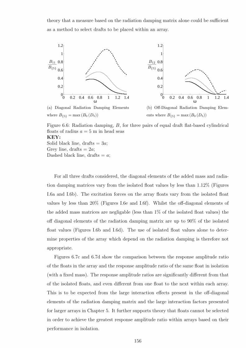
theory that a measure based on the radiation damping matrix alone could be sufficient
as a method to select drafts to be placed within an array.
0 0.2 0.4 0.6 0.8 1 1.2 1.40
0.2
0.4
0.6
0.8
1
1.2
ω
B11
B5
(a) Diagonal Radiation Damping Elements
where B5 = max (B0 (D5))
0 0.2 0.4 0.6 0.8 1 1.2 1.40
0.2
0.4
0.6
0.8
1
1.2
ω
B12
B5
(b) Off-Diagonal Radiation Damping Elem-
ents where B5 = max (B0 (D5))
Figure 6.6: Radiation damping, B, for three pairs of equal draft flat-based cylindricalfloats of radius a = 5 m in head seasKEY:Solid black line, drafts = 3a;Grey line, drafts = 2a;Dashed black line, drafts = a;
For all three drafts considered, the diagonal elements of the added mass and radia-
tion damping matrices vary from the isolated float values by less than 1.12% (Figures
I.6a and I.6b). The excitation forces on the array floats vary from the isolated float
values by less than 20% (Figures I.6e and I.6f). Whilst the off-diagonal elements of
the added mass matrices are negligable (less than 1% of the isolated float values) the
off diagonal elements of the radiation damping matrix are up to 90% of the isolated
float values (Figures I.6b and I.6d). The use of isolated float values alone to deter-
mine properties of the array which depend on the radiation damping is therefore not
appropriate.
Figures 6.7c and 6.7d show the comparison between the response amplitude ratio
of the floats in the array and the response amplitude ratio of the same float in isolation
(with a fixed mass). The response amplitude ratios are significantly different from that
of the isolated floats, and even different from one float to the next within each array.
This is to be expected from the large interaction effects present in the off-diagonal
elements of the radiation damping matrix and the large interaction factors presented
for larger arrays in Chapter 5. It further supports theory that floats cannot be selected
in order to achieve the greatest response amplitude ratio within arrays based on their
performance in isolation.
156
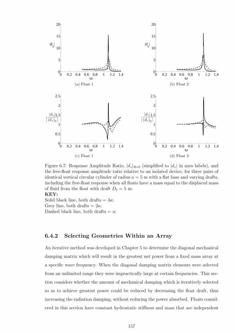
0 0.2 0.4 0.6 0.8 1 1.2 1.40
5
10
15
20
ω
|dz|
(a) Float 1
0 0.2 0.4 0.6 0.8 1 1.2 1.40
5
10
15
20
ω
|dz|
(b) Float 2
0 0.2 0.4 0.6 0.8 1 1.2 1.40
0.5
1
1.5
2
2.5
ω
|dz|| (dz)0 |
(c) Float 1
0 0.2 0.4 0.6 0.8 1 1.2 1.40
0.5
1
1.5
2
2.5
ω
|dz|| (dz)0 |
(d) Float 2
Figure 6.7: Response Amplitude Ratio, |dz|R=0 (simplified to |dz| in axes labels), andthe free-float response amplitude ratio relative to an isolated device, for three pairs ofidentical vertical circular cylinder of radius a = 5 m with a flat base and varying drafts,including the free-float response when all floats have a mass equal to the displaced massof fluid from the float with draft D5 = 5 m:KEY:Solid black line, both drafts = 3a;Grey line, both drafts = 2a;Dashed black line, both drafts = a;
6.4.2 Selecting Geometries Within an Array
An iterative method was developed in Chapter 5 to determine the diagonal mechanical
damping matrix which will result in the greatest net power from a fixed mass array at
a specific wave frequency. When the diagonal damping matrix elements were selected
from an unlimited range they were impractically large at certain frequencies. This sec-
tion considers whether the amount of mechanical damping which is iteratively selected
so as to achieve greatest power could be reduced by decreasing the float draft, thus
increasing the radiation damping, without reducing the power absorbed. Floats consid-
ered in this section have constant hydrostatic stiffness and mass that are independent
157
of draft.
The initial (base) array for which the iteratively determined optimal diagonal me-
chanical damping matrix is determined is a 2× 1 array of equal draft flat-based cylin-
ders. Whilst several alternative drafts can be considered to replace the base array,
the selection method must require as few calculations as possible. For the selection
of drafts with equal hydrostatic stiffness and mass, the radiation damping has been
shown to vary significantly more with draft than the added mass or excitation force.
The use of the radiation damping alone to determine the most appropriate draft of
cylinder at each wave frequency is therefore considered in this section.
The base array have drafts of 3a where the radius a = 5 m. Two alternative drafts
of 2a and a are considered. The radiation damping generally increases with decreasing
draft.
The total damping on an array of power absorbing floats is given by the sum of the
mechanical and radiation damping matrices such that FD = R + B. As R is a 2 × 2
diagonal matrix and B a 2 × 2 dense matrix, the total damping on each float of the
base array for unit response is given as the sum of each row of FD which is written as
Ωi = Ri,i +Bi,i +Bi,j (6.3)
for i, j ∈ 1, 2. All elements of Ωi = Ri,i + Bi,i + Bi,j are known, since the matrix, R,
is the iteratively selected mechanical damping matrix. For every draft, D, (including
the base array and each alternative draft pair) the sum of the ith row of the radiation
damping matrix is known and defined as
Θi(D) = Bi,i +Bi,j. (6.4)
For each draft, the mechanical damping elements, Ri,i, can be calculated such that
Ri,i(D) = Ωi −Θi(D). (6.5)
Ri,i(D) represents the total damping on float i of the base array minus the total radi-
ation damping on float i of the pair of floats with draft D.
For the base array this will result in the iteratively selected mechanical damping
values, whereas for the alternative draft pairs it will result in new mechanical damping
values. The purpose of selecting a draft is to minimise the mechanical damping required
158

without reducing the power. Applying negative mechanical damping to floats is likely
to reduce the net power absorbed however. At each frequency, only the drafts for
which Ri,i is non-negative on both floats will therefore be considered. The mechanical
damping for each draft, D, is therefore given by
Ri,i(D) =
Ωi −Θi(D) if Ωi ≤ Θi(D)
NaN if Ωi > Θi(D)(6.6)
where NaN (Not-a-Number) represents an invalid entry (see Figure 6.8). It is the net
mechanical damping which must be minimised, which is given for each draft, D, by
2∑
i=1
Ri,i(D) =
∑2i=1 (Ωi −Θi(D)) if Ωi ≤ Θi(D) for both of i = 1, 2
NaN if Ωi > Θi(D) for either of i = 1, 2. (6.7)
The criterion by which the pair of floats with drafts Ds are selected at a particular
wave frequency is therefore
Ds selected ⇐⇒ It is the draft for which2∑
i=1
Ri,i(Ds) is smallest. (6.8)
Any drafts for which∑N
i=1 Ri,i is an invalid entry (NaN) are not included in the range
of drafts considered.
0 0.2 0.4 0.6 0.8 1 1.2 1.40
5
10
15
20
ω
Θ1
(a) Θ < Ω, Float 1
0 0.2 0.4 0.6 0.8 1 1.2 1.40
5
10
15
20
ω
Θ2
(b) Θ < Ω, Float 2
Figure 6.8: Θ (as given by Equation (6.4)) for pairs of equal draft cylindrical floats ofradius a and drafts of D = 3a (thick, solid, black line), D = 2a (grey line) and D = a(Dashed line) at all frequencies where Θ < Ω, where Ω is given by Equation (6.3) (Thinblack line)
The drafts selected using criterion (6.8) are shown in Figure 6.9. At frequencies far
from the natural frequency, the shallowest draft pair of floats (D = a) are selected as
these have the largest radiation damping. As the magnitude of the iteratively selected
159

damping values are reduced closer to the peak frequency, the total radiation damping
(Θ) on the shallowest draft pair of floats is greater than the total damping on the base
array (Ω). The selected draft is therefore increased to D = 2a in this frequency range.
At frequencies very close to the peak, the iteratively selected damping values are less
than the radiation damping (Θ) on both of the alternative draft pairs, so the base array
(D = 3a) is selected.
0 0.2 0.4 0.6 0.8 1 1.2 1.40
1
2
3
ω
D
Figure 6.9: Draft D (relative to a) selected to minimise required mechanical dampingfrom the base array without reducing net power (Selected using Criterion (6.8) in whichthe mechanical damping is determined using Equation (6.6))
The net power absorbed by drafts selected in this way is predominantly greater than
or equal to the net power from the base array with the optimum diagonal mechanical
damping matrix (Figure 6.10a). At frequencies in the ranges 1.05 ≤ ω ≤ 1.055 rad/sec
and 1.88 ≤ ω ≤ 1.91 rad/sec however, the power is reduced by up to 88% compared
to the base array by using drafts a and 2a respectively which are selected according
to condition (6.6). On closer inspection, Ri,i of the selected draft, although the least
out of the three drafts, are extremely small compared to the equivalent iteratively
selected mechanical damping value at these frequencies. A further condition must
therefore be included in the selection criteria such that the mechanical damping values
of the selected drafts must not only be non-negative, but must be at least 32% of the
equivalent iteratively selected mechanical damping values. The draft selection criterion
therefore becomes
Ri,i(D) =
Ωi −Θi(D) where Ωi−Θi(D)
R[b]i,i
≥ 0.32
NaN where Ωi−Θi(D)
R[b]i,i
< 0.32. (6.9)
Applying the mechanical damping values calculated using Equation (6.9) within
the selection criterion (Equation (6.8)) results in the selection of drafts for which the
160

net power is always at least as great as the base arrays, whilst the mechanical damping
is less than or equal to the base array (Figure 6.10b)
0 0.2 0.4 0.6 0.8 1 1.2 1.40
500
1000
1500
2000
2500
ω
Pnet%
(a) Drafts selected using mechanical damping
(6.6)
0 0.2 0.4 0.6 0.8 1 1.2 1.40
500
1000
1500
2000
2500
ω
Pnet%
(b) Drafts selected using mechanical damping
(6.9)
Figure 6.10: Percentage increase,(P%net
), in Net Power of the drafts selected using
criterion (6.8) compared to the base array
Where the optimal diagonal mechanical damping matrix is known for a pair of
floats at one draft therefore, it is possible at some frequencies to reduce the mechanical
damping whilst increasing the net power by varying the draft of the floats. Furthermore,
it is possible to select the most appropriate draft for each wave frequency using only
knowledge of the base array’s optimal diagonal mechanical damping matrix and the
radiation damping matrix for each alternative draft.
Further Work
The draft selection for a small array in which both floats have equal draft is considered
in this section. A method has been presented to determine which pair of floats would
be most appropriate at each wave frequency, where the optimal mechanical damping
is known for only one pair of floats. The study has been performed using a choice of
only three drafts of floats. It would be beneficial to continue the study to select from
a larger range of floats, and a range of floats in which the drafts are not equal within
each pair.
The hydrodynamic parameters are determined using WAMIT. In order to allow
pairs of floats in which the drafts are not equal, the WAMIT geometry definition file
first needs to be modified. Once the study has been extended in this way, the same
method can be used to select geometries to be placed within larger arrays using theory
of Direct-Neighbour Coupling as discussed in Section 6.1.
161

Application to a larger array, would require the optimal diagonal mechanical damp-
ing matrix to be iteratively determined for a Base Array of equal draft floats. Suppose
the floats are numbered with increasing magnitude such that float 1 is the front float,
float 2 the float directly adjacent to it and so on. The front float (float 1) could then
be fixed so that its draft does not change from the base draft. During the small array
study, the mechanical damping matrices for the Alternative Draft Pairs would have
been determined for every combination of drafts within a 2 × 1 array. Based on the
Direct-Neighbour Coupling, floats 1 and 2 can then be considered as if they were a
2× 1 array. Based on float 1’s performance within a 2× 1 array, the most appropriate
draft for float 2 can be selected. Floats 2 and 3 can then be considered as if they are a
2× 1 array, hence float 3’s draft selected. The process can be repeated until the drafts
of all floats within the array have been selected.
6.5 Chapter Conclusion
Variations in submerged geometry cause variations in added mass, radiation damp-
ing and excitation force as well as hydrostatic stiffness if the water-plane area varies
between geometries. Application of geometry variation to match the incident wave
conditions is best applied through the variation of draft. The masses of the bodies can
either be kept constant and independent of mass, or be dependent on draft such as
when the floats are neutrally buoyant.
Submerged geometry changes which are closest to the free surface have the most
significant effect on the hydrodynamic parameters. A geometry, referred to as ConTop,
in which large variations in submerged geometry can be achieved with only small
changes in draft is therefore defined and analysed at varying depths in isolation.
The power absorbed by a float at a particular wave frequency is calculated in linear
theory as a function of the added mass, excitation force, radiation damping, hydrostatic
stiffness, float mass and mechanical damping. Where the water-plane area, hence
hydrostatic stiffness remains constant, the variation with draft of radiation damping
is much greater than that of the added mass or excitation force. This suggests that
where the desired total damping is known, such as the total damping which will result
in the greatest power, the radiation damping is the best indicator of which draft is
most appropriate.
The free float response accounts for a variation in all of the parameters which are
required to calculate the power except for the mechanical damping. It would therefore
162

be desirable to use the free float response as a method to select the drafts which
will result in the greatest power without prior knowledge of the mechanical damping
values. Where the masses of the floats are draft-dependent, the natural frequency varies
significantly and consistently with draft. Where this is the case, the free-float response
is a good indicator of the drafts which result in the greatest power at a particular wave
frequency, regardless of the mechanical damping value. Where the mass is constant and
independent of mass however, there is little correlation between the free-float response
and the power absorbed. Where the mass is constant and the mechanical damping
value large, the shallower draft floats are found to absorb the greatest power over
much of the frequency range.
Where the draft can be varied in accordance with each incident wave frequency,
large magnitudes in power can be achieved across a large range of frequencies. The
frequency bandwidths over which a large amount of power can be absorbed by each
draft can however be small for some drafts. A small variation in incident wave frequency
could therefore result in a significant drop in power. A new measure, χ, which combines
the magnitude and standard deviation of the power is therefore developed to determine
the suitability of a float for power absorption over a specific range of wave frequencies.
In certain frequency ranges, χ is found to select a float which achieves a similar power
to that which, if floats were selected to achieve the greatest power at each individual
wave frequency, would have required a large range of float geometries.
The interactions within an array are found to be most significant between directly
adjacent floats for the five element linear array analysed in Section 5. It is therefore
possible that float drafts could be varied within an array based only on knowledge of
each float’s interaction within a two element array with its direct neighbour. This is a
theory termed Direct-Neighbour Coupling.
Interactions of three pairs of equal draft cylindrical floats are analysed. As with
the isolated bodies, the radiation damping is found to vary more significantly with
draft than the added mass or excitation force. Further to this, the diagonal elements
of the radiation damping matrix are found to vary significantly with draft and be only
slightly smaller in magnitude than the diagonal elements.
Where the optimal diagonal mechanical damping matrix is known for a pair of
floats at one draft, it is possible at some frequencies to reduce the mechanical damping
whilst increasing the net power by varying the draft of the floats. Furthermore, it
is possible to select the most appropriate draft for each wave frequency using only
knowledge of the base array’s optimal diagonal mechanical damping matrix and the
163
radiation damping matrix for each alternative draft. This method is only valid where
the water-plane area and hence the hydrostatic stiffness remain constant.
A study in which this method could be used to select drafts within a large array is
proposed. In this study, the first float’s draft would be fixed. Based on the first floats
performance in a two element array, the directly adjacent float would be selected and
fixed. The process would be repeated until the drafts of each element in the array are
selected.
164

Chapter 7
Conclusion
7.1 Overview
This thesis focuses on the modelling of closely spaced groups (arrays) of wave energy
devices which each use vertical (heaving) motion to generate electricity. The main
aims are to determine the limitations of the applicability of the model, obtain accurate
predictions of their behaviour in different sea conditions and determine realistically
attainable optimal characteristics.
A mathematical model is presented which combines linear wave theory with a series
of linear driven harmonic oscillators to model an array of floating wave energy devices
in a train of incident regular waves. Under the assumption of small amplitude waves,
the velocity potential is expanded into a perturbation series, of which linear wave
theory considers only the terms of the first order. Although it has previously been
shown using linear wave theory that large interaction factors may occur at certain
combinations of device spacing to the wavelength of regular waves, much of the existing
work does not address array configurations or device constraints that are relevant to
designers of structure-supported array devices. Specifically, much of the published work
addresses relatively large inter-device spacing and optimal mass and damping matrices
are typically applied.
The suitability of linear wave theory for application to closely spaced arrays is
assessed in this thesis through comparison to small-scale experimental data and to a
numerical model in which second-order effects are included. The experimental compar-
ison is performed for the response of a five element array of free-floating hemispherical
floats. Power take-off (through the application of a damping force) is not considered
in the experimental comparison in order to provide the most stringent test for linear
wave theory by permitting large amplitude motions. The second-order comparison is
165

performed for a two element array in which the forces calculated using linear wave
theory (first order) are compared to those calculated using terms of the perturbation
series up to the second order.
The linear theory model is used to determine the behaviour of a realistic closely
spaced array in which float mass cannot change significantly and damping is determined
independently of the motion of the other floats within the array and is applied to only
the heave oscillation of each float. The maximum power and hence interaction factors
that are achievable from fixed geometry arrays in regular seas are thus determined.
Variation of submerged float geometry alters several hydrodynamic parameters at
once. The variation of submerged float geometry to manipulate both the power and the
magnitude of mechanical damping which needs to be applied to achieve the power is
considered. The study is performed through analysis of both simple uniform geometries
and a unique complex geometry in isolation, and analysis of the performance of simple
uniform geometries at different drafts within a small array.
7.2 Mathematical Conclusions
This section considers the findings from this thesis which are most interesting from a
mathematical modelling perspective. The same equation which is commonly used to
calculate power for an isolated device is shown to be applicable to arrays of devices
provided the mechanical damping matrix is diagonal. This presents a method to de-
termine not only the net power from an array of devices, but also the individual float
power outputs.
A new Normalised Interaction Factor, Q, is introduced which gives the power ab-
sorbed by devices within an array relative to the maximum power from the same num-
ber of isolated devices with set mass and mechanical damping values. This provides a
more meaningful measure of performance for the purpose of comparison between de-
vices with different characteristics than the interaction factor q that has traditionally
been used to define array performance.
A further new measure, χ, is introduced in this thesis to determine the optimal
float (from a selection of floats) for power absorption over a specific range of wave
frequencies. This measure considers both the mean and standard deviation of the
power over the specified range of wave frequencies. In certain frequency ranges, χ is
found to select one float from a range of floats which achieves a similar power to that
which, if floats were selected to achieve the greatest power at each individual wave
166

frequency, would have required a large number of different floats from the same range.
A time series of second-order forces is determined from interpolated non-dimensional
forces which are made dimensional using wave amplitudes as calculated from a wave
spectrum together with random phases. A convergence study is conducted and it is
found that second-order wave forces are insignificant within a frequency range specific
to the incident wave spectrum, but are greater than or equal to 10 % of the first-order
forces at frequencies outside of this range. Quadratic equations for the limit frequencies
of this range are presented in this thesis in terms of the significant wave height and the
peak period of the incident wave spectrum.
7.3 Engineering Conclusions
This section gives a brief discussion of the main conclusions which are most relevant
from the perspective of device developers. Whilst linear theory has been shown to follow
the same general trends as experimental results, linear theory models in which a small
amount of mechanical damping is included despite the floats being free-floating is found
to provide a better fit to experimental data. The magnitude of the damping that is
not accounted for in the linear hydrodynamic model could be attributed to a number
of physical processes that are typically assumed negligible. These phenomena may
include slight differences of geometry between individual floats causing both variations
in the hydrodynamic parameters and variations in the scaling (since the scaling factor
is based on the float diameter only); the effects of the tank walls causing variations
in the radiation damping compared to the open sea case; variations of inter-device
spacing that occur in the experiments due to motions in modes which are not included
in the numerical model (i.e. in surge); variations in the immersed surface resulting in
variations in forcing; and non-linear variations in hydrostatic restoring forces due to
non-vertical sides of the floats and large changes in immersed volume during motion.
Care must therefore be taken when considering results from both experimental and
numerical models, to understand their limitations and assumptions when compared to
the final design.
Whilst linear wave theory is applicable to closely spaced arrays in many situations,
it excludes all terms of the velocity potential which are higher than first order. The
second-order forces are considered in this thesis for a variety of sea states which are
determined to be relevant to closely spaced arrays of wave energy devices. Whilst the
second-order effects can be significant at low and high frequencies, for most sea states
167
they are insignificant (< 10 % of first order) for much of the range of wave frequencies
which closely spaced arrays of wave energy devices are likely to be subjected. Within
this important frequency range, it is only at low frequencies when the peak period is
large (≥ 11.5 seconds) and at high frequencies when the peak period is small (≤ 7.5
seconds) that second-order effects must be taken into consideration. An increase in
significant wave height increases the ratio of second to first-order forces such that
second-order forces must also be considered at higher frequencies when the peak period
is ≥ 9.5 seconds.
Much published numerical data based on linear wave theory indicates extremely
large magnitudes of net power can be absorbed from devices when placed within an
array environment compared to when placed in isolation. This data commonly requires
highly complex systems to apply the optimal forcing to the devices. A more reasonable
system is considered in this thesis in which the floats have a fixed mass and the me-
chanical damping force is applied to each float independently of the motion of the other
floats. For a five element linear array, close to the natural frequency of the devices,
where the maximum power is attained for the realistic arrays, the reduction in power
compared to the fully optimal arrays is determined to be approximately 3 % in beam
seas and 18 % in head seas. Under the restriction that mechanical damping of any
one float cannot be dependent on the motion of any other float, the greatest power is
achieved by selecting mechanical damping values individually and independently of the
radiation damping. For the array in beam seas, power output is found to be greatest
when alternate floats are nearly stationary. In head seas, maximum power output is
obtained at low wavenumbers if mechanical damping is increased with row number.
In contrast, at high wavenumbers, net power output is maximum when damping is
greatest on the front float. The peak in net power occurs at a slightly higher wave
frequency in head seas than beam seas, with the magnitude of net power at the peak
being approximately 4 % greater in head than beam seas. At frequencies below these
peaks, the net power is slightly greater in head than beam seas. At frequencies greater
than these peaks however, the net power is significantly greater in beam seas.
Application of geometry variation to match the incident wave conditions is best
applied through the variation of draft. Submerged geometry changes which are closest
to the free surface have the most significant effect on the hydrodynamic parameters.
For neutrally buoyant wave energy devices for which float mass is draft dependent, the
free-float response can be used to indicate the draft which will result in the greatest
power under the application of an unknown quantity of mechanical damping.
168

Where the mass of the floats is to remain constant (i.e. systems with a counter
mass or positively buoyant systems), the radiation damping varies significantly more
between drafts than the other hydrodynamic parameters, provided the water-plane
area remains constant (i.e. straight-sided axisymmetric floats). When straight-sided
axisymmetric floats of fixed mass are placed in isolation, the shallower draft floats are
found to absorb the greatest power over much of the frequency range provided the
mechanical damping value is large. Where the optimal mechanical damping values are
known for an array of straight-sided axisymmetric floats of fixed mass, the required
mechanical damping can be reduced at most wave frequencies by varying the draft of
individual devices without compromising the net power output.
7.4 Future Work
Several topics addressing the application of linear wave theory to closely spaced arrays
and the realistically achievable optimal characteristics of floats within an array have
been addressed in this thesis. Whilst each topic is investigated thoroughly and useful
findings obtained, they each introduce new topics and questions to be answered. This
section gives an overview of several extensions to the thesis which would be interesting
to pursue.
The motions noticeable in alternative modes in the wave tank are determined in
this thesis to be one of the main contributing factors to the discrepancies between the
calculated and experiment magnitudes of response due to the resulting variations in
inter-float spacing. A variation of the numerical model in which small motions are
permitted in alternative modes would clarify the extent to which these small motions
cause these discrepancies. The comparison would be similar in form to the single-mode
of motion comparison presented in this thesis, with hydrodynamic parameters obtained
from a wave analysis programme (such as WAMIT).
At certain wave frequencies dependent on the sea state, second-order forces are
determined in this thesis to be significant within a closely spaced array. The extension
to the current model in which multiple modes of motion are permitted could also include
second-order response amplitude ratios. The first and second-order non-dimensional
response amplitude ratios can also be obtained using a wave analysis programme such
as WAMIT and analysed within the model. This more detailed analysis would allow
for more precise determination of the frequency ranges over which linear theory is
appropriate for use on closely spaced arrays, and offer a more thorough comparison
169

between linear wave theory and experimental data for closely spaced arrays.
The use of free-float response in the comparison between experimental data and
linear wave theory in this thesis represents the most extreme test for linear wave theory
in terms of amplitudes of float motion and eliminates the need to model a power take-
off system. Power values within closely spaced arrays determined using linear wave
theory are presented throughout this thesis for different float characteristics. In order
to determine the accuracy of these predictions a power take-off system would need to
be modelled in the numerical model. Power take-off systems are predominantly non-
linear in that they apply mechanical damping for only parts of the wave cycles. In
order to include a power take-off system in the numerical calculations, a time-varying
model would be required.
The mechanical damping applied in the linear theory calculations in this thesis
are the time-averaged values at each wave frequency. The time-varying model could
still calculate the float performance in the frequency domain where required through
transformation using an FFT. In this way, it could be determined whether a close
approximation to the non-linear power take-off system could be made based on time-
averaged values in the frequency domain. If a suitable approximation does exist, then
a frequency domain model could be used to determine float performance with much
higher computational efficiency than a time-domain model. This would also clarify the
appropriateness of existing published results in the frequency domain.
The interactions within an array are found to be most significant between directly
adjacent floats for a five element linear array. A theory termed direct neighbour cou-
pling is therefore presented in this thesis suggesting that float drafts could be varied
within a large array based only on knowledge of each floats interaction within a two ele-
ment array with its direct neighbour. Where the floats are numbered sequentially from
one to N for a linear N -element array such that float 1 is the front float, the geometry
of float 1 could be fixed. Based on the most appropriate two-element array in which the
front float had the same geometry as float 1, the geometry of float 2 could be selected
and fixed. Similarly, based on the most appropriate two element array in which the
front float is the same geometry as float 2, float 3 could be determined. This process
could be continued until all N elements of the large array have been determined. A
procedure would thus be developed in which the optimal geometries to be placed at
each position within an array could be determined using only the optimal diagonal
mechanical damping matrix for the large array and the knowledge of the interactions
of each geometry in a two element array.
170
In this thesis, drafts are selected from a range of only three drafts (including the
original draft) for two element arrays in which both floats within the same array have
the same draft. In order to implement the procedure to determine the optimum geome-
try for each position in a large array, the range of drafts considered should be increased
from three to at least ten to improve the accuracy of the results. Every combination
of two drafts would need to be analysed to determine the hydrodynamic parameters
such that pairs of floats of unequal drafts are also considered. The layout of the array
would be linear with fixed, predetermined spacings.
171

Appendix A
Mathematical Identities
The following are mathematical identities which have been relied upon in this thesis.
The symbols, x, y, γ, Z1 and Z2 used in this section are arbitrary and do not correspond
to any similar symbols used throughout the thesis.
Trigonometric Sum and Product Rules:
cos(x± y) = cos(x) cos(y)∓ sin(x) sin(y) (A.1)
cosh(x± y) = cosh(x) cosh(y)± sinh(x) sinh(y) (A.2)
Exponential Representations:
eix = cos (x) + i sin (x) (A.3)
Integrals:
∫ π
0
cos (γ cosx) dx = πJ0 (|γ|) when γ ∈ < (A.4)
∫ π
0
sin (γ cosx) dx = 0 when γ ∈ < (A.5)
Infinite Series:
J0 (γ) = 1− γ2
(1!)2 · 22+
γ4
(2!)2 · 24+ · · · =
∞∑
n=0
(−1)n γ2n
(n!)2 · 22n(A.6)
sinh (γ) = γ +γ3
3!+γ5
5!+γ7
7!+ · · · =
∞∑
n=0
γ2n+1
(2n+ 1)!(A.7)
cosh (γ) = 1 +γ2
2!+γ4
4!+γ6
6!+ · · · =
∞∑
n=0
γ2n
(2n)!(A.8)
172
Complex Numbers:
For complex numbers Z1 and Z2 with complex conjugates Z∗1 and Z∗2 , if
Z1 =1
2(Z2 + Z∗2) then Z1 = <Z2. (A.9)
173
Appendix B
Complex Amplitudes
In linear wave theory all oscillations are assumed to be sinusoidal. As a steady state
condition is assumed in linear wave theory, there cannot be any transient effects
present due to initial conditions. As a result, the linear motions and loads on the
body are assumed to oscillate harmonically at the same frequency as the wave loads
which excite the body (Faltinsen, 1990, P.39). Using complex representations of these
parameters is therefore convenient. The main advantage to using complex amplitudes
is that the multiplication of a complex amplitude with iω gives the differential of the
complex amplitude.
The forces acting on a floating body are assumed to vary sinusoidally with time with
an angular frequency of ω with phase constant ϕ and so can be written as
F = |F | cos (ωt+ ϕ) . (B.1)
Using exponential representation (A.3), this can be written as
F = <|F |ei(ωt+ϕ)
= <
|F |eiωteiϕ
. (B.2)
Introducing the complex potential of the force, F , this can be written as
F = <F eiωt
, (B.3)
where
F = |F |eiϕ = |F | cos(ϕ) + i|F | sin(ϕ). (B.4)
174

Using the complex number rule given by equation (A.9), the force can alternatively
be written as
F =1
2
(F eiωt + F ∗e−iωt
). (B.5)
The displacement, velocity and acceleration of the body can all be written in terms of
their complex amplitudes.
It is worth noting that the absolute amplitude of the complex amplitude is equal to
the amplitude of the oscillation such that |F | = |F |.
175
Appendix C
Defining Geometries in WAMIT
The wave analysis programme, WAMIT, can be used to compute the modulus, phase,
real and imaginary parts of various parameters such as the excitation force, added
mass, damping, hydrodynamic pressure, and body velocity for specific body
geometries in a train of incident waves.
WAMIT contains a lower order method and a higher order method (obtained by
setting ILOWH = 0 and 1 respectively in the configuration file). The lower order
method involves splitting the body surface into panels. The velocity and the source
strength can then be approximated by piecewise constant values on each panel. In
the higher order method, the body is represented by ‘patches’ which are smooth,
continuous surfaces in space. The velocity potential on the body is then represented
by B-Splines in a continuous manner, and the fluid velocity can be evaluated by
analytical differentiation.
When using the higher order method there is an option to use explicit, analytical
representation of certain body geometries of the body written in Fortran. This means
that the representation of the body geometry is exact and so the only numerical
calculation remaining is in the calculation of the velocity potential. For these specific
geometries, WAMIT is able to very quickly compute the hydrodynamic parameters.
The geometries included in the WAMIT distribution of this geometry definition file
include a flat-based circular cylinder, a flat-based elliptical cylinder, a semi-immersed
sphere, an ellipsoid, a torus, a Tension Leg Platform, and a ship’s hull among others.
Each explicitly defined geometry has a small selection of parameters which can be
varied, such as the radius and the draught.
Modification of the FORTRAN file in which the geometries are explicitly defined
allows for the inclusion of user-defined explicit definitions of alternative geometries.
The hemispherical and flat-based-cylindrical floats used throughout this thesis are
176

defined explicitly using the original, WAMIT distribution of the geometry definition
file. The more unusual geometries of a hemispherical-based cylinder and ConTop
which are studied in Chapter 6 are defined explicitly using patches. The geometry
definition file included within WAMIT is modified to include the additional
definitions of these geometries at varying depths. The geometry definition is validated
by comparison to WAMIT parameters obtained using the lower order method
obtained by further definitions of these geometries as lists of panel vertices.
177
Appendix D
Analytical Froude-Krylov Force
The double integrals in Equation (2.43) can be solved analytically using the Bessel
function of the first kind and some well known identities.
The only term in the integrand of Equation (2.43) which includes the variable θ is
cos(k a sinψ cos θ − ω t), which can be expanded using the identity (A.1) to give
FFKz =ρ g Ha2
2 cosh(k d)
∫ π/2
0
∫ 2π
0
cos(k a sinψ cos θ) cos(ω t)
+ sin(k a sinψ cos θ) sin(−ω t)
dθ
× cosh(k(d− a cosψ)) cosψ sinψ
dψ.
The inner integrand can be solved using identities (A.4) and (A.5) along with the
symmetry of the body to give
FFKz =ρ g Ha2
2 cosh(k d)
∫ π/2
0
2πJ0 (k a sinψ) cos(ω t)
× cosh(k(d− a cosψ)) cosψ sinψ
dψ,
where J0 represents the Bessel function of the first kind. As it is the time-averaged
force that is of interest, this can be written as
FFKz =πρ g Ha2
cosh(k d)
∫ π/2
0
J0 (k a sinψ)
× cosh(k(d− a cosψ)) cosψ sinψ
dψ. (D.1)
Using the identity (A.2), the integrand expands to give
FFKz =πρ g Ha2
cosh(k d)
∫ π/2
0
J0 (k a sinψ)
×
cosh(kd) cosh(ka cosψ)
− sinh(kd) sinh(ka cosψ)
cosψ sinψ
dψ.
178
The terms J0 (k a sinψ), sinh(ka cosψ) and cosh(ka cosψ) can be expanded to their
infinite series using (A.6), (A.7) and (A.8) to give
FFKz =πρ g Ha2
cosh(k d)
∫ π/2
0
∑∞n=0
(−1)n(k a sinψ)2n
(n!)2·22n
×
cosh(kd)
∑∞n=0
(ka cosψ)2n
(2n)!
− sinh(kd)∑∞
n=0(ka cosψ)2n+1
(2n+1)!cosψ sinψ
dψ.
Expanding the infinite series to the order of 10 and integrating gives
FFKz =πρ g Ha2
cosh(k d)(γ2 cosh (kd) + γ3 sinh (kd)) , (2.44)
Where
γ2 =
1 + a2k2
8− a4k4
576+ a6k6
46080− a8k8
5160960+ a10k10
796262400− 29a12k12
78033715200
+ a14k14
249707888640− 53a16k16
337105649664000+ a18k18
6742112993280000− a20k20
148326485852160000
and
γ3 =
− 6758061133824000 ak+ 39070080 a11k11
− 868224 a13k13+ 19152 a15k15− 42 a17k17+ a19k19
· 1
10137091700736000.
179
Appendix E
Numerical Froude-Krylov Force
Equation (2.43) can be evaluated numerically using the composite trapezoidal rule
twice.
E.1 The Composite Trapezoidal Rule
The composite trapezoidal rule approximates the definite integral of a function, f(x),
as the sum of several trapeziums. This is achieved by dividing the domain into n+ 1
discrete points such that −→x = x0, x1, x2, · · · , xn−1, xn, where x0 and xn are the limits
of the integration and δx = xi+1 − xi is the increment size, and calculating the
function at each. The integral of the function between each adjacent pair in the
domain,∫ xi+1
xif(x)dx, can be approximated by the area of a trapezium with vertices
(xi, 0), (xi, f(xi)), (xi+1, 0) and (xi+1, f(xi+1)) such that
Area of Trapezium =1
2(f (xi+1) + f (xi)) δx.
These areas can be summed to approximate the integral between the limits x0 and xn:
∫ xn
x0
f(x)dx =
(1
2(f(x0) + f(xn)) +
n−1∑
i=1
f (xi)
)δx. (E.1)
E.2 Application to Equation (2.43)
Equation (2.43) contains a double integral whose domain contains both θ and ψ. The
angles θ and ψ must be divided into n sections of size δθ and m sections of size δψ
180
respectively such that
−→θ = [0, δθ, 2δθ, · · · , (θn−2)δθ, 2π]
and−→ψ = [0, δψ, 2δψ, · · · , (ψm−2)δψ,
π
2δψ].
The body surface is thus divided into panels of finite size, dSb = a2 sinψδθδψ.
Equation (2.43) can be rewritten as
FFKz =ρ g Ha2
2 cosh(k d)
∫ π/2
0
∫ 2π
0
I (θ, ψ) dθdψ,
where I (θ, ψ) is the integrand given by
I (θ, ψ) = cosh(k(d− a cosψ)) cos(k a sinψ cos θ − ω t) cosψ sinψ.
Applying the composite trapezoidal rule twice gives
FFKz =ρ g Ha2
2 cosh(k d)
((1
2(G (θ, ψ0) +G (θ, ψn)) +
m−1∑
i=1
G (θ, ψi)
)δψ
), (2.45)
where
G (θ, ψi) =
(1
2(I (θ0, ψi) + I (θn, ψi)) +
n−1∑
j=1
I (θj, ψi)
)δθ.
181
Appendix F
Derivation of the Full Power
Equation (2.49)
The mechanical power, P , of a moving body is a function of the external force, Fext,
on the body multiplied by the body’s velocity, U :
P (t) = Fext(t)U(t).
Fext and U can alternatively be written in terms of their complex amplitudes using
Equation (B.5) to give
P (t) =1
4
(Fexte
iωt + F ∗exte−iωt)(
Ueiωt + U∗e−iωt)
=1
4
(FextUe
i2ωt + F ∗extU∗ei2ωt + F ∗extU + FextU
∗), (F.1)
in which the superscript symbol, ‘∗’, represents the complex conjugate. The first two
terms of this expansion, FextUei2ωt + F ∗extU
∗ei2ωt, represents an oscillating quantity
with complex amplitude FextU and frequency 2ω which when averaged over time is
zero. The time averaged power is therefore given by
P =1
4
(F ∗extU + FextU
∗). (F.2)
Using Equation (B.3) this can be rewritten as
P =1
2<F ∗extU
. (2.47)
182

The external force comes from the waves and so is the sum of the excitation force, Fe,
and radiation force, Fr, (see Section 2.2.2). Using Equation (2.34) the power can
therefore be written as
P =1
2<(F ∗e − U∗
(B − iωA
))U
=1
2<F ∗e U
− 1
2<U∗(B − iωA
)U
=1
2<F ∗e U
− 1
2U∗BU. (F.3)
Expanding the complex amplitudes into their real and imaginary parts results in
P =
1
2<
<Fe
<U
+ =Fe
=U
−i=Fe
<U
+ i<Fe
=U
− B
2
(<U)2
+(=U)2
+i<U=U− i=
U<U
. (F.4)
Now consider a set of terms, Cz, which equate to zero when summed together:
Cz =
18(B)
((<Fe
)2
−(<Fe
)2)
+ 18(B)
((=Fe
)2
−(=Fe
)2)
+i 18(B)
(=Fe
<Fe
−=
Fe
<Fe
)
= 0. (F.5)
Cz can be added to Equation (F.4) without affecting the value of P , so that the terms
can be rearranged to give Equation (2.49):
P =1
8F ∗eB
−1Fe −1
2
(U− 1
2B−1Fe
)∗B
(U− 1
2B−1Fe
).
183
Appendix G
Statistical Measures
In order to mathematically define the statistical measures used in Section 3.4, let the
sum over all wave frequencies and all floats be represented by Sum such that
Sum =Nω∑
i=1
N∑
j=1
. (G.1)
Furthermore, let the experimental and calculated response amplitude ratios be
represented by zE and zC respectively such that
zE =∣∣d[E]z (i, ω(j))
∣∣ (G.2)
and zC =∣∣d[C]z (i, ω(j))
∣∣ , (G.3)
where∣∣∣d[E]z (i, ω(j))
∣∣∣ represents the experimental- and∣∣∣d[C]z (i, ω(j))
∣∣∣ represents the
numerical- response amplitude ratio of body i at frequency ω(j). Also let a line above
a character denote its mean value such that the mean value of the experimental data
is given by:
zE =Sum (zE)
Nω ·N=
∑Nω
i=1
∑Nj=1
∣∣∣d[E]z (i, ω(j))
∣∣∣Nω ·N
. (G.4)
The statistical measures considered in this section can therefore be defined as:
the Mean Absolute Error,
MAE =Sum (|zE − zC |)
Nω ·N, (G.5)
184

the Root Mean Square Error,
RMSE =
√Sum ((zE − zC)2)
Nω ·N, (G.6)
the Mean Absolute Percentage Error,
MAPE = 100× 1
Nω ·N
( |zE − zC |zE
), (G.7)
the Root Mean Square Percentage Error,
RMSPE = 100×√
1
Nω ·NSum
(((zE − zC)2)
zE
), (G.8)
the Mean Absolute Error as a Percentage of the Experimental Mean,
MAEPM =100
zE× Sum (|zE − zC |)
Nω ·N, (G.9)
the Root Mean Square Error as a Percentage of the Experimental Mean,
RMSEPM =100
zE×√Sum ((zE − zC)2)
Nω ·N, (G.10)
the Coefficient of Residual Mass,
CRM =Sum(zE)− Sum(zC)
Sum(zE), (G.11)
the Difference in Variance Ratio,
DV R =Sum (zE − zE)− Sum (zC − zC)
Sum (zE − zE), (G.12)
the Maximum Error between any predicted value and its corresponding actual value,
ME = max (zE − zC) , (G.13)
185
the Coefficient of Determination,
CD =Sum
((zE − zE)2)
Sum((zE − zC)2) , (G.14)
and the modelling efficiency,
EF =Sum (zE − zE)− Sum (zC − zE)
Sum (zE − zE). (G.15)
The MAE (Mean Absolute Error) gives mean error of the calculated data as a model
of the experimental data. The RMSE (Root Mean Square Error) is similar, but
considers the squares of the errors, thus making large errors more significant. Both
the MAE and the RMSE are given in the same units as the input data, so their
values are specific to the case being considered and so useful mainly for comparing
similar models. Their values however could not be used to compare the application of
models to different variables with different units. It can therefore be useful to give a
measure of the error as a percentage of the actual experimental data such as in the
MAPE (Mean Absolute Percentage Error), RMSPE (Root Mean Square Percentage
Error), MAEPM (Mean Absolute Error as a Percentage of the experimental Mean)
and RMSEPM (Root Mean Square Error as a Percentage of the experimental
Mean). Care must be taken when considering MAPE and RMSPE as they are
sensitive to small experimental values, with singularities given for experimental values
of zero. When comparing these four percentage measures of error it is worth
considering how, since these represent percentages, a small value at a frequency near
the peak frequency can correspond to a large difference between the calculated and
experimentally measured values.
The CRM gives the difference between the means of the experimental and calculated
values as a ratio of the mean experimental value. Variance indicates the magnitude of
the spread of data about its mean value. DV R gives the difference in the variances of
the experimental and calculated values relative to the variance of the experimental
data. The CD indicates to what extent the spread of the calculated data can explain
the variance of the experimental data. EF is suggested to be one of the most
important indicators of overall good fit (Mayer and Butler, 1993) with a negative
value indicating a model which cannot be recommended as this suggests simply using
the mean of the experimental data at all frequencies would be a better model (Loague
and Green, 1991).
186

Together with the statistical values for overall fit of the calculated data to the
experimental data it is useful to determine the worst case which is given by ME.
187
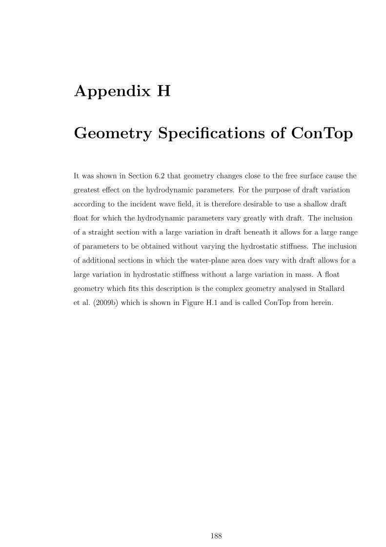
Appendix H
Geometry Specifications of ConTop
It was shown in Section 6.2 that geometry changes close to the free surface cause the
greatest effect on the hydrodynamic parameters. For the purpose of draft variation
according to the incident wave field, it is therefore desirable to use a shallow draft
float for which the hydrodynamic parameters vary greatly with draft. The inclusion
of a straight section with a large variation in draft beneath it allows for a large range
of parameters to be obtained without varying the hydrostatic stiffness. The inclusion
of additional sections in which the water-plane area does vary with draft allows for a
large variation in hydrostatic stiffness without a large variation in mass. A float
geometry which fits this description is the complex geometry analysed in Stallard
et al. (2009b) which is shown in Figure H.1 and is called ConTop from herein.
188
Figure H.1: Diagram of complex geometry called ConTop:Patch 1 = horizontal circular base of radius a1 = 2.21 m;Patch 2 = lower outer-quadrant of torus with radius a2 = a3− a1 = 2.79 m and heightL2 = a2;Patch 3 = vertical circular cylinder of radius a3 = 5 m and height L3 = 3.07 m;Patch 4 = conical section of height L4 = 1.74 m;Patch 5 = vertical circular cylinder of radius a4 = 1.67 m and height L5 = 3.83 m;Patch 6 = horizontal circular lid of radius a4 = 1.67 m
The ConTop geometry consists of a cylindrical section of small radius at the top,
below which is a conical section, below which is another cylindrical section of larger
radius, below which is the lower outer-quadrant of a torus at the base of which is a
flat, circular base. The geometry is defined in WAMIT analytically as a series of
patches which are smooth and continuous in space (see appendix C). The
specifications (based on an experimental model) and the patches used to define the
geometry analytically are shown in Figure H.1. In this thesis the ConTop geometry is
analysed at different drafts to determine the effect of the draft variation on different
hydrodynamic parameters.
Fifteen drafts of the ConTop geometry are analysed. The drafts are labelled DX for
X = α, β, γ, δ, ε, ζ, η, A, B, C, D, E, F , G and H as shown in Figure H.2.
189

Figure H.2: Diagram of ConTop Geometry with Drafts labelled such that free surfaceis located along the straight section in still water :Dα = draft when free surface is located at α: Dα = L2 + L3 + L4 + L5;Dβ = draft when free surface is located at β: Dβ = L2 + L3 + L4 + 0.5L5;Dγ = draft when free surface is located at γ: Dγ = L2 + L3 + L4;Dδ = draft when free surface is located at δ: Dδ = L2 + L3 + 0.8L4;Dε = draft when free surface is located at ε: Dε = L2 + L3 + 0.6L4;Dζ = draft when free surface is located at ζ: Dζ = L2 + L3 + 0.4L4;Dη = draft when free surface is located at η: Dη = L2 + L3 + 0.2L4;DA = draft when free surface is located at A: DA = L2 + L3;DB = draft when free surface is located at B: DB = L2 + 0.8L3;DC = draft when free surface is located at C: DC = L2 + 0.6L3;DD = draft when free surface is located at D: DD = L2 + 0.4L3;DE = draft when free surface is located at E: DE = L2 + 0.2L3;DF = draft when free surface is located at F : DF = L2;DG = draft when free surface is located at G: DG = 0.8L2;DH = draft when free surface is located at H: DH = 0.6L2
190
Appendix I
Variation of Hydrodynamic
Parameters with Float Draft
Basic hydrodynamic parameters are presented in this section in relation to the
geometries considered in Chapter 6. Each geometry is considered at a variety of
depths to determine the dependence of each of the hydrodynamic parameters on the
draft.
I.1 Isolated Geometries
I.1.1 Flat-Based Cylinder
The first geometry to consider is a flat based cylinder of radius a and draft 3a, 2a or a.
As the draft of the flat-based cylinder is increased, the radiation damping and
excitation force are decreased, and the added mass is decreased at lower frequencies
and increased at higher frequencies.
The maximum ratio of added mass, radiation damping and excitation force from one
draft of flat-based cylinder to the next are 1.2, 58.6 and 7.7 respectively. All of these
maximum ratios occur at the largest frequency within the specified range
(0.49 ≤ ω ≤ 1.4 rad/sec). The mean across all frequencies of the largest ratios (at
each frequency) from one flat-based cylinder to the next are 1.1, 12.1 and 3.1 for the
added mass, radiation damping and excitation force respectively.
191

0 0.2 0.4 0.6 0.8 1 1.2 1.40
0.5
1
1.5
2
2.5
3x 10
5
ω
A
(a) Added Mass
0 0.2 0.4 0.6 0.8 1 1.2 1.40
1
2
3
4
5
6x 10
4
ω
B
(b) Radiation Damping
0 0.2 0.4 0.6 0.8 1 1.2 1.40
1
2
3
4
5
6
x 105
ω
F
(c) Excitation Force
Figure I.1: Hydrodynamic parameters for a vertical circular cylinder of radius a = 5m with a flat base with length, l:KEY:Solid black line, l = 3a; Grey line, l = 2a; Dashed black line, l = a
I.1.2 Hemispherical-Based Cylinder
The hemispherical-based cylinder considered in this section consists of a straight
vertical section of radius a and length l = 3a, 2a or a, and a hemispherical base of
radius a. The total drafts considered are therefore 4a, 3a and 2a.
The general trends of the variation of hydrodynamic parameters with draft are the
same as for the flat-based cylinder. The magnitudes of the hydrodynamic parameters
are however reduced when compared to the flat-based cylinder whose draft is the
same length as the straight section of the hemispherical-based cylinder.
192
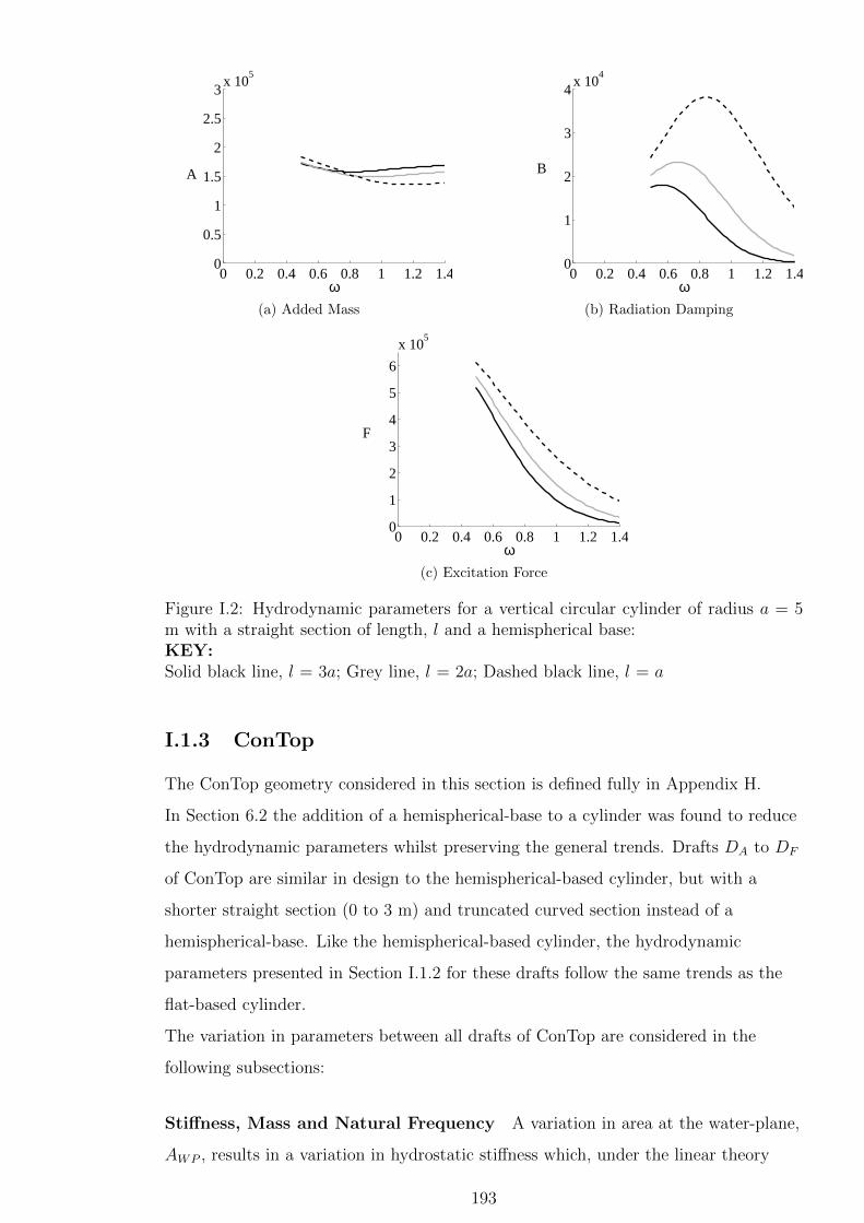
0 0.2 0.4 0.6 0.8 1 1.2 1.40
0.5
1
1.5
2
2.5
3x 10
5
ω
A
(a) Added Mass
0 0.2 0.4 0.6 0.8 1 1.2 1.40
1
2
3
4x 10
4
ω
B
(b) Radiation Damping
0 0.2 0.4 0.6 0.8 1 1.2 1.40
1
2
3
4
5
6
x 105
ω
F
(c) Excitation Force
Figure I.2: Hydrodynamic parameters for a vertical circular cylinder of radius a = 5m with a straight section of length, l and a hemispherical base:KEY:Solid black line, l = 3a; Grey line, l = 2a; Dashed black line, l = a
I.1.3 ConTop
The ConTop geometry considered in this section is defined fully in Appendix H.
In Section 6.2 the addition of a hemispherical-base to a cylinder was found to reduce
the hydrodynamic parameters whilst preserving the general trends. Drafts DA to DF
of ConTop are similar in design to the hemispherical-based cylinder, but with a
shorter straight section (0 to 3 m) and truncated curved section instead of a
hemispherical-base. Like the hemispherical-based cylinder, the hydrodynamic
parameters presented in Section I.1.2 for these drafts follow the same trends as the
flat-based cylinder.
The variation in parameters between all drafts of ConTop are considered in the
following subsections:
Stiffness, Mass and Natural Frequency A variation in area at the water-plane,
AWP , results in a variation in hydrostatic stiffness which, under the linear theory
193
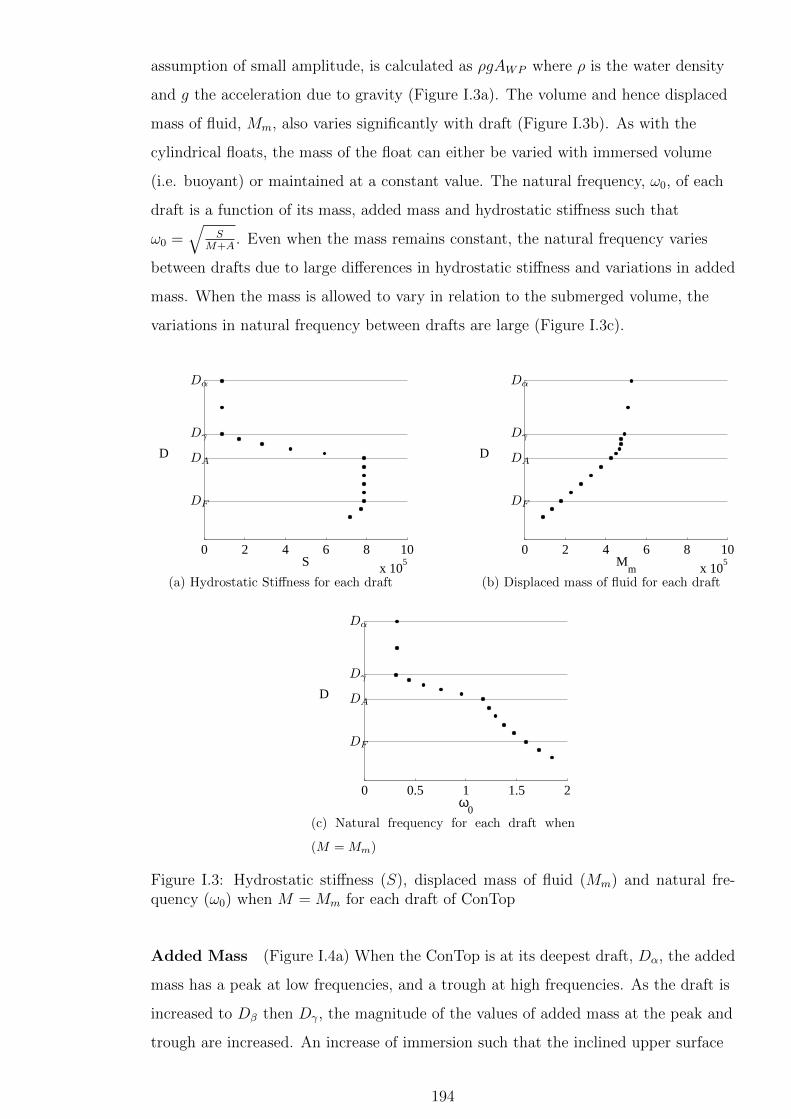
assumption of small amplitude, is calculated as ρgAWP where ρ is the water density
and g the acceleration due to gravity (Figure I.3a). The volume and hence displaced
mass of fluid, Mm, also varies significantly with draft (Figure I.3b). As with the
cylindrical floats, the mass of the float can either be varied with immersed volume
(i.e. buoyant) or maintained at a constant value. The natural frequency, ω0, of each
draft is a function of its mass, added mass and hydrostatic stiffness such that
ω0 =√
SM+A
. Even when the mass remains constant, the natural frequency varies
between drafts due to large differences in hydrostatic stiffness and variations in added
mass. When the mass is allowed to vary in relation to the submerged volume, the
variations in natural frequency between drafts are large (Figure I.3c).
0 2 4 6 8 10
x 105S
D
DF
DA
Dγ
Dα
(a) Hydrostatic Stiffness for each draft
0 2 4 6 8 10
x 105M
m
D
DF
DA
Dγ
Dα
(b) Displaced mass of fluid for each draft
0 0.5 1 1.5 2ω
0
D
DF
DA
Dγ
Dα
(c) Natural frequency for each draft when
(M = Mm)
Figure I.3: Hydrostatic stiffness (S), displaced mass of fluid (Mm) and natural fre-quency (ω0) when M = Mm for each draft of ConTop
Added Mass (Figure I.4a) When the ConTop is at its deepest draft, Dα, the added
mass has a peak at low frequencies, and a trough at high frequencies. As the draft is
increased to Dβ then Dγ, the magnitude of the values of added mass at the peak and
trough are increased. An increase of immersion such that the inclined upper surface
194
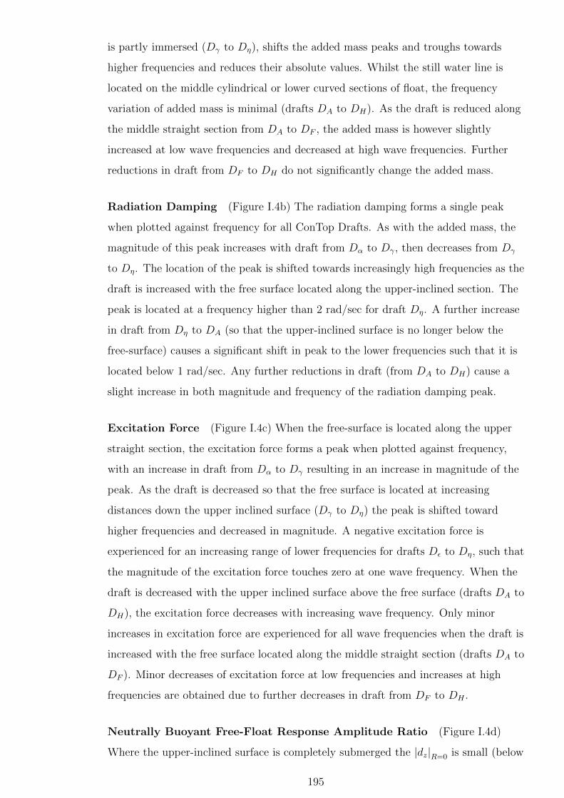
is partly immersed (Dγ to Dη), shifts the added mass peaks and troughs towards
higher frequencies and reduces their absolute values. Whilst the still water line is
located on the middle cylindrical or lower curved sections of float, the frequency
variation of added mass is minimal (drafts DA to DH). As the draft is reduced along
the middle straight section from DA to DF , the added mass is however slightly
increased at low wave frequencies and decreased at high wave frequencies. Further
reductions in draft from DF to DH do not significantly change the added mass.
Radiation Damping (Figure I.4b) The radiation damping forms a single peak
when plotted against frequency for all ConTop Drafts. As with the added mass, the
magnitude of this peak increases with draft from Dα to Dγ, then decreases from Dγ
to Dη. The location of the peak is shifted towards increasingly high frequencies as the
draft is increased with the free surface located along the upper-inclined section. The
peak is located at a frequency higher than 2 rad/sec for draft Dη. A further increase
in draft from Dη to DA (so that the upper-inclined surface is no longer below the
free-surface) causes a significant shift in peak to the lower frequencies such that it is
located below 1 rad/sec. Any further reductions in draft (from DA to DH) cause a
slight increase in both magnitude and frequency of the radiation damping peak.
Excitation Force (Figure I.4c) When the free-surface is located along the upper
straight section, the excitation force forms a peak when plotted against frequency,
with an increase in draft from Dα to Dγ resulting in an increase in magnitude of the
peak. As the draft is decreased so that the free surface is located at increasing
distances down the upper inclined surface (Dγ to Dη) the peak is shifted toward
higher frequencies and decreased in magnitude. A negative excitation force is
experienced for an increasing range of lower frequencies for drafts Dε to Dη, such that
the magnitude of the excitation force touches zero at one wave frequency. When the
draft is decreased with the upper inclined surface above the free surface (drafts DA to
DH), the excitation force decreases with increasing wave frequency. Only minor
increases in excitation force are experienced for all wave frequencies when the draft is
increased with the free surface located along the middle straight section (drafts DA to
DF ). Minor decreases of excitation force at low frequencies and increases at high
frequencies are obtained due to further decreases in draft from DF to DH .
Neutrally Buoyant Free-Float Response Amplitude Ratio (Figure I.4d)
Where the upper-inclined surface is completely submerged the |dz|R=0 is small (below
195

1) with a slight peak in response at low wave frequencies followed by a decrease in
neutrally buoyant |dz|R=0 with increasing frequency. An decrease in draft from Dα to
Dγ results in an increase in |dz|R=0 at all wave frequencies. Extreme peaks (of 38, 80
and 15 for Dε, Dζ and Dη respectively) in |dz|R=0 are predicted when the free surface
is located at the upper inclined surface, with a decrease in draft corresponding to an
increase in the frequency at which the extreme peak is located. For these same drafts
|dz|R=0 is zero at a slightly higher frequency than the peak. When the draft is
increased so that the upper-inclined surface is completely above the free surface, the
peaks in the |dz|R=0 curves are no longer extreme (below 4.5) and do not decrease to
zero immediately after the peak frequency. As the draft is decreased from DA to DH ,
the location of the peak is moved to an increasingly high wave frequency, and its
magnitude is increasingly reduced.
The extreme peaks predicted when the free surface is located at the upper-inclined
surface (drafts Dε to Dη) could be due to motion trapped modes which are coupled
oscillations of the body and the fluid which would not decrease with time in the
absence of viscosity (McIver and McIver, 2007). The extreme peaks are predicted as
a result of the limited radiation damping calculated close to their natural frequencies.
In practice, the extreme peaks would not occur however due to the additional forces
which would be present for these drafts due to sloshing, wave breaking and viscous
effects which are not included within the linear model (Stallard et al., 2009b).
196

0 0.5 1 1.5 2
0
2
4
6
8x 10
5
ω
A
(a) Added Mass
0 0.5 1 1.5 20
2
4
6
8
10x 10
5
ω
B
(b) Radiation Damping
0 0.5 1 1.5 20
2
4
6
8
10
x 105
ω
F
(c) Excitation Force
0 0.5 1 1.5 20
1
2
3
4
5
ω
|dz|
(d) Neutrally Buoyant Free-Float Response
Amplitude Ratio (max |za| = 38)
Figure I.4: Hydrodynamic parameters for ConTop at various drafts defined in FigureH.2:KEY:Thick Solid black line, draft Dγ; Solid grey line, draft Dε;Thin dashed line, draft DA; Thin Solid black line, draft DC ;Dotted black line, draft DF ; Thick dashed line, draft DH
I.2 Array of Flat-Based Cylinders
The hydrodynamic parameters for the cylindrical bodies discussed in Section I.1.1 are
presented here within a two-element array. The parameters are given relative to fixed
values in Figure I.5, and relative to the equivalent isolated value at the same wave
frequency in Figure I.6.
197

0 0.2 0.4 0.6 0.8 1 1.2 1.40
0.2
0.4
0.6
0.8
1
1.2
ω
A11
A5
(a) Diagonal Added Mass Elements where
A5 = max (A0 (D5))
0 0.2 0.4 0.6 0.8 1 1.2 1.40
0.2
0.4
0.6
0.8
1
1.2
ω
A12
A5
(b) Off-Diagonal Added Mass Elements where
A5 = max (A0 (D5))
0 0.2 0.4 0.6 0.8 1 1.2 1.40
0.2
0.4
0.6
0.8
1
ω
F1
F5
(c) Excitation Force on Float 1 where F5 =
max (F0 (D5))
0 0.2 0.4 0.6 0.8 1 1.2 1.40
0.2
0.4
0.6
0.8
1
ω
F2
F5
(d) Excitation Force on Float 2 where F5 =
max (F0 (D5))
Figure I.5: Hydrodynamic parameters for three pairs of identical, cylindrical floats:KEY:Solid black line, both flat-based cylindrical floats with drafts = 3a;Grey line, both flat-based cylindrical floats with drafts = 2a;Dashed black line, both flat-based cylindrical floats with drafts = a
198

0 0.2 0.4 0.6 0.8 1 1.2 1.40.6
0.8
1
1.2
1.4
ω
A11
A0
(a) Diagonal Added Mass Elements
0 0.2 0.4 0.6 0.8 1 1.2 1.40
0.02
0.04
0.06
0.08
0.1
ω
A12
A0
(b) Off-Diagonal Added Mass Elements
0 0.2 0.4 0.6 0.8 1 1.2 1.40.6
0.8
1
1.2
1.4
ω
B11
B0
(c) Diagonal Radiation Damping Elements
0 0.2 0.4 0.6 0.8 1 1.2 1.40
0.2
0.4
0.6
0.8
1
ω
B12
B0
(d) Off-Diagonal Radiation Damping Ele-
ments
0 0.2 0.4 0.6 0.8 1 1.2 1.40.6
0.8
1
1.2
1.4
ω
F1
F0
(e) Excitation Force on Float 1
0 0.2 0.4 0.6 0.8 1 1.2 1.40.6
0.8
1
1.2
1.4
ω
F2
F0
(f) Excitation Force on Float 2
Figure I.6: Hydrodynamic parameters (relative to frequency and draft dependent iso-lated device parameters) for three pairs of identical vertical circular cylinder of radiusa = 5 m with a flat base and varying drafts:KEY:Solid black line, both drafts = 3a;Grey line, both drafts = 2a;Dashed black line, both drafts = a;
199

Appendix J
Relationship Between Response
and Power
In this appendix, the free-float response is shown for both flat-based cylinders and
ConTop at a variety of drafts. Also shown is the net power which is absorbed by each
draft when different values of mechanical damping are applied.
J.0.1 Flat-Based Cylinder
This section considers three drafts of flat-based cylinder with radius a and draft 3a,
2a or a.
Where the mass is allowed to vary according to the draft, the peaks in the power
curves for each draft are found close to their natural frequencies, resulting in the
range of wave frequencies over which each draft results in the greatest power being
very similar to those of greatest free-float response (Figures J.1a and J.1c).
Where the mass is constant, all methods used to calculate the mechanical damping
result in the shallower draft floats achieving the greatest power for all frequencies,
except very close to the peak when R = Ropt (figure J.1d). The same relationship is
however not found for the free-float response (Figure J.1b).
200
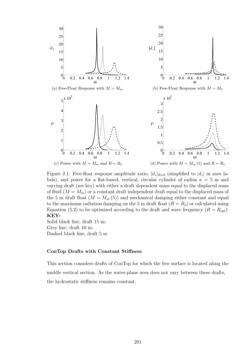
0 0.2 0.4 0.6 0.8 1 1.2 1.40
5
10
15
20
25
30
(a) Free-Float Response with M = Mm
0 0.2 0.4 0.6 0.8 1 1.2 1.40
5
10
15
20
25
30
(b) Free-Float Response with M = M5
0 0.2 0.4 0.6 0.8 1 1.2 1.40
1
2
3
4
5x 10
5
ω
P
(c) Power with M = Mm and R = R5
0 0.2 0.4 0.6 0.8 1 1.2 1.40
0.5
1
1.5
2
2.5
3x 10
5
ω
P
(d) Power with M = Mm (5) and R = R5
Figure J.1: Free-float response amplitude ratio, |dz|R=0 (simplified to |dz| in axes la-bels), and power for a flat-based, vertical, circular cylinder of radius a = 5 m andvarying draft (see key) with either a draft dependent mass equal to the displaced massof fluid (M = Mm) or a constant draft independent draft equal to the displaced mass ofthe 5 m draft float (M = Mm (5)) and mechanical damping either constant and equalto the maximum radiation damping on the 5 m draft float (R = R5) or calculated usingEquation (5.2) to be optimised according to the draft and wave frequency (R = Ropt):KEY:Solid black line, draft 15 m;Grey line, draft 10 m;Dashed black line, draft 5 m
ConTop Drafts with Constant Stiffness
This section considers drafts of ConTop for which the free surface is located along the
middle vertical section. As the water-plane area does not vary between these drafts,
the hydrostatic stiffness remains constant.
201

0 0.5 1 1.5 20
1
2
3
4
5
ω
|dz|
(a) Free-Float Response with M = Mm)
0 0.5 1 1.5 20
1
2
3
4
5
ω
|dz|
(b) Free-Float Response with M = MDF
0 0.5 1 1.5 20
5
10
15x 10
4
ω
P
(c) Power with M = Mm and R = RDF
0 0.5 1 1.5 20
5
10
15x 10
4
ω
P
(d) Power with M = MDFand R = RDF
Figure J.2: Free-float response amplitude ratio, |dz|R=0 (simplified to |dz| in axeslabels), and power for geometry ConTop at drafts Dγ, Dε, DA, DC , DF and DH
(see Figure H.2) with either a draft-dependent mass equal to the displaced massof fluid (M = Mm) or a constant draft-independent mass equal to the displacedmass of the float with draft DF (M = Mm (DF ) = MDF
) and mechanical dampingconstant and equal to the maximum radiation damping on the float with draft DF
(R = max (B (DF )) = RDF):
KEY: Thick Solid black line, draft DA; Solid grey line, draft DB;Thin dashed line, draft DC ; Thin Solid black line, draft DD;Dotted black line, draft DE; Thick dashed line, draft DF
Whilst the magnitude of the peak in free-float response increases with draft, the
bandwidth (that is the range of frequencies over which the free-float response is large)
decreases with draft (see Figure J.2b).
At low and high wave frequencies the optimal mechanical damping values for the
constant mass floats decrease with decreasing draft, and close to the natural wave
frequencies, the optimal mechanical damping values increase with decreasing draft.
For any constant mechanical damping value, the larger the draft of the float, the
greater the under-damping at low and high wave frequencies (due to the greater
difference between the constant and optimal mechanical damping values at those
frequencies). A large constant mechanical damping value therefore minimises the
202
under-damping at low and high wave frequencies, but over-damps the deeper draft
floats near the peak frequency. This results in the larger draft floats experiencing a
larger bandwidth and lower peak power value when the mechanical damping value is
large, so that the smaller draft float achieves the greatest power across the whole
frequency range. A small constant mechanical damping value however, results in the
larger draft floats being even more under-damped at low and high frequencies and
closer to their optimum values near the peak frequency, reducing the bandwidth and
increasing the peak. The large difference between drafts of both the peaks and
bandwidths results in different drafts achieving the greatest power at different wave
frequencies.
Drafts with Varying Stiffness
The second set of ConTop drafts is a selection of drafts covering the whole geometry
therefore allowing variations in the water-plane area hence stiffness. For this purpose
the free-float response and power output for drafts Dγ, Dε, DA, DC , DF and DH are
compared in this section.
203
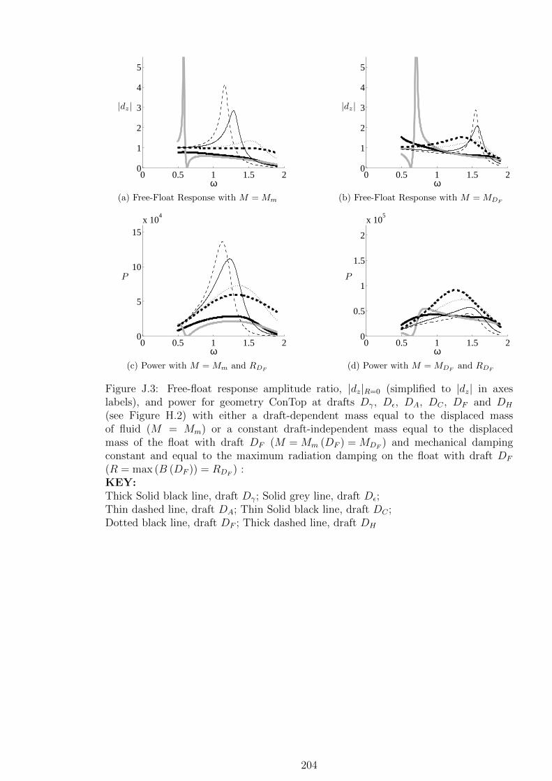
0 0.5 1 1.5 20
1
2
3
4
5
ω
|dz|
(a) Free-Float Response with M = Mm
0 0.5 1 1.5 20
1
2
3
4
5
ω
|dz|
(b) Free-Float Response with M = MDF
0 0.5 1 1.5 20
5
10
15x 10
4
ω
P
(c) Power with M = Mm and RDF
0 0.5 1 1.5 20
0.5
1
1.5
2
x 105
ω
P
(d) Power with M = MDFand RDF
Figure J.3: Free-float response amplitude ratio, |dz|R=0 (simplified to |dz| in axeslabels), and power for geometry ConTop at drafts Dγ, Dε, DA, DC , DF and DH
(see Figure H.2) with either a draft-dependent mass equal to the displaced massof fluid (M = Mm) or a constant draft-independent mass equal to the displacedmass of the float with draft DF (M = Mm (DF ) = MDF
) and mechanical dampingconstant and equal to the maximum radiation damping on the float with draft DF
(R = max (B (DF )) = RDF) :
KEY:Thick Solid black line, draft Dγ; Solid grey line, draft Dε;Thin dashed line, draft DA; Thin Solid black line, draft DC ;Dotted black line, draft DF ; Thick dashed line, draft DH
204
Bibliography
Abuk-Azm, A. G., Williams, A. N., 1988a. Second-order diffraction loads on truncated cylin-
ders. Journal of Waterways, Port, Coastal and Ocean Division, 436–454.
Abuk-Azm, A. G., Williams, A. N., 1988b. Second-order diffraction loads on two uniform
vertical cylinders. In: Proceedings 7th International Offshore Mechanics and Arctic Engi-
neering Conference. Houston, Texas, U.S.A., pp. 131–138.
Abuk-Azm, A. G., Williams, A. N., 1989a. Approximation of second-order diffraction loads
on vertical cylinder arrays. Journal of Fluids and Structures, 17–36.
Abuk-Azm, A. G., Williams, A. N., 1989b. Second-order diffraction loads on arrays of semi-
immersed cylinders. Journal of Fluids and Structures, 365–388.
Al-Habaibeh, A., Su, D., McCaguec, J., Knight, A., 2010. An innovative approach for energy
generation from waves. Energy Conversion and Management 51, 1664–1668.
American Society of Civil Engineers Task Committee on Hydrology Handbook, 1996. Hy-
drology handbook, 2nd Edition. ASCE Publications.
Aquamarine Power, March 2011. Official website for Oyster wave power device.
URL http://www.aquamarinepower.com/
AW-Energy Oy, March 2011. Official website for WaveRoller wave energy converter.
URL http://www.aw-energy.com/
AWS Ocean Energy Ltd, March 2011. Official website for Archimedes Wave Swing wave
energy converter.
URL http://www.awsocean.com/home.aspx
Babarit, A., Clement, A., 2006. Optimal latching control of a wave energy device in regular
and irregular waves. Applied Ocean Research 28, 77–91.
Babarit, A., Duclos, G., Clement, A. H., 2004. Comparison of latching control strategies for
a heaving wave energy device in random sea. Applied Ocean Research, 227–238.
205
Bellew, S., Stallard, T., 2010. Linear modelling of wave device arrays and comparison to
experimental and second order models. In: Proceedings 25th International Workshop on
Water Waves and Floating Bodies. pp. 9–12.
Bellew, S., Stallard, T., Stansby, P., 2009. Optimisation of a heterogeneous array of heaving
bodies. In: Proceedings of the 8th European Wave and Tidal Energy Conference. Uppsala,
Sweden, pp. 519–527.
Bjarte-Larsson, T., Falnes, J., Moan, T., 2006. Comparison of results from time-domain
simulations and model tests of a water-pumping wave-power unit. In: Proceedings of 16th
Offshore and Polar Engineering Conference. pp. 417–422.
Boake, C. B., Whittaker, T. J. T., Folley, M., 2002. Overview and initial operational ex-
perience of the limpet wave energy plant. In: Proceedings of The Twelfth International
Offshore and Polar Engineering Conference. pp. 586–594.
Brito-Melo, A., Neumann, F., Sarmento, A., 2008. Full-scale data assessment in OWC pico
plant. International Journal of Offshore and Polar Engineering 18, 27–34.
Brooke, J., 2003. Wave Energy Conversion. Elsevier Science Ltd.
Budal, K., Dec 1977. Theory for absorption of wave power by a system of interacting bodies.
JSR 21 (4), 248–253.
Budal, K., Falnes, J., Kyllingstad, A., Oltedal, G., 1979. Experiments With Point Absorbers.
Chalmers University of Technology, Gothenburg, Sweden.
Butler, B. P., Thomas, G. P., 1993. The diffraction of water waves by an array of circular
cylinders in a channel. Ocean Engineering 20 (3), 295–311.
Callan, M., Linton, C., Evans, 1991. Trapped modes in two-dimensional wave guides. Journal
of Fluid Mechanics 229, 51–64.
Chakrabarti, S. K., Tam, W. A., 29 April-2 May 1973. Gross and wave load on a large vertical
cylinder - theory and experiment. In: Proceedings of the 5th Annual Offshore Technology
Conference. Houston, Texas.
Chaplin, R. V., Rahmati, M. T., Gunura, K., Ma, X., Aggidis, G. A., 2009. Control systems
for wraspa. In: Proceedings of the International Conference on Clean Electrical power.
Capri, Italy, pp. 93 – 97.
Chau, F. P., Eatock Taylor, R., 1988. Second order velocity potential for arbitrary bodies in
waves. In: Third International Workshop on Water Waves and Floating Bodies.
206

Chau, F. P., Eatock Taylor, R., 1992. Second order wave diffraction by a vertical cylinder.
Journal of Fluid Mechanics 240, 571–599.
Clement, A., McCullen, P., Falcao, A., Fiorentino, A., Gardner, F., Hammarlund, K., Lemo-
nis, G., Lewis, T., Nielsen, K., Petroncini, S., Teresa Pontes, M., Schild, P., Sjostrom,
B.-O., Sørensen, H. C., Thorpe, T., 2002. Wave energy in europe: Current status and
perspectives. Renewable and Sustainable Energy Reviews, 405–431.
Count, B. M., November 1978. On the dynamics of wave-power devices. In: Proceedings
of the Royal Society of London. Vol. 363 of A, Mathematical and Physical Sciences. pp.
559–579.
Count, B. M. Jefferys, E. R., Tokyo 1980. Wave power: The primary interface. In: Proceedings
of the 13th Symposium on Naval Hydrodynamics. pp. 817–826.
Cruz, J., 2008. Ocean Wave Energy: Current Status and Future Prespectives. Springer.
Cruz, J., Sykes, R., Siddorn, P., Eatock Taylor, R., 2009. Wave farm design: Preliminary
studies on the influences of wave climate, array layout and farm control. In: Proceedings
of the 8th European Wave and Tidal Energy Conference. pp. 736–745.
de Backer, G., Vantorre, M., Beels, C., De Rouck, J., Frigaard, P., 2009. Performance of
closely spaced point absorbers with constrained floater motion. In: Proceedings of the 8th
European Wave and Tidal Energy Conference. pp. 806–817.
de Rouck, J., Meirschaert, V., 2009. Sustainable economically efficient wave energy converter
(seewec) publishable final activity report. Tech. rep., University of Ghent.
URL http://www.seewec.org/results/Publishable%20final%20activity%20report.
Draper, M., 2006. More than just a ripple: Ocean power technologies sets its sights high.
Refocus, 54–56.
Eatock Taylor, R., Huang, J. B., 1997a. Second-order wave diffraction by an axisymmetric
body in monochromatic waves. In: The Royal Society Proceedings: Mathematical, Physical
and Engineering Sciences. Vol. 453. pp. 1515–1541.
Eatock Taylor, R., Huang, J. B., 1997b. Semi-analytical formulation for second-order diffrac-
tion by a vertical cylinder in bichromatic waves. Journal of Fluids and Structures 11,
465–484.
Eatock Taylor, R., Hung, S. I., 1987. Second-order diffraction forces on a vertical cylinder.
Applied Ocean Research, 19–30.
207

Eatock Taylor, R., Hung, S. I., Chau, F. P., 1989. On the distribution of second order pressure
on a vertical circular cylinder. Applied Ocean Research 11 (4).
Evans, D. V., 1979. Some theoretical aspects of three-dimensional wave-energy absorbers. In:
Proceedings of the 1st Symposium on Wave-Energy Utilisation. Gothenburg.
Evans, D. V., Jeffrey, D. C., Salter, S. H., Taylor, J. R. M., 1979a. Submerged cylinder wave
energy device: Theory and experiment. Applied Ocean Research 1.
Evans, D. V., Jeffrey, D. H., Salter, S. H., Taylor, J. R. M., 1979b. Submerged cylinder wave
energy device: Theory and experiment. Applied Ocean Research 1 (1).
Evans, D. V., Linton, C. M., 1991. Trapped modes in open channels. Journal of Fluid Me-
chanics 225, 153–175.
Falcao, A. F. d. O., 2008. Phase control through load control of oscillating-body wave energy
converters with hydraulic PTO system. Applied Ocean Research, 358–366.
Falcao, A. F. d. O., 2010. Wave energy utilization: A review of the technologies. Renewable
and Sustainable Energy Reviews 4, 899–918.
Falcao, A. F. d. O., Justino, P. A., Henriques, J. C., Andre, J. M. C. S., 2009. Reactive versus
latching phase control of a two-body heaving wave energy converter. In: Proceedings of
the European Control Conference. Budapest, Hungary, pp. 3731–3736.
Falnes, J., 1980. Radiation impedance matrix and optimum power absorption for interacting
oscillators in surface waves. Applied Ocean Research 2, 75–80.
Falnes, J., 2002. Ocean Waves and Oscillating Systems: Linear Interactions Including Wave-
Energy Extraction. Cambridge University Press, Cambridge.
Falnes, J., 2007. A review of wave-energy extraction. Marine Structures 20, 185–201.
Falnes, J., Lillebekken, P. M., 2003. Budal’s latching-controlled-buoy type wave-power plant.
In: Proceedings of the 5th European Wave Energy Conference 2003. pp. 233–244.
Faltinsen, O. M., 1990. Sea Loads on Ships and Offshore Structures. Cambridge University
Press, Cambridge.
Fitzgerald, C., Thomas, G., 2007. A preliminary study on the optimal formation of an array
of wave power devices. In: Proceedings of the 7th European Wave and Tidal Energy
Conference. Porto, Portugal.
Frigaard, P., Lyke Anderson, T., 2008. Effektmalinger pa Wave Star i nissum bredning. Tech.
Rep. 61, Aalborg University, , Denmark.
208
Garcia-Rosa, P., Cunha, J., Lizarralde, F., Estefen, S., Costa, P., 2009. Efficiency optimiza-
tion in a wave energy hyperbaric converter. In: Proceedings of the International Conference
on Clean Electrical Power. pp. 68 – 75.
GEOS, F., 2001. Wind and wave frequency distributions for sites around the british isles.
Tech. rep., Health and Safety Executive.
Ghalayini, S. A., Williams, A. N., 1991. Nonlinear wave forces on vertical cylinder arrays.
Journal of Fluids and Structures 5, 1–32.
Goda, Y., 2000. Random Seas and Design of Maritime Structures, 2nd Edition. World Sci-
entific Publishing Co. Pte. Ltd.
Greenhow, M., Vinje, T., Brevig, P., Taylor, J., 1982. A theoretical and experimental study
of the capsize of Salters Duck in extreme waves. Journal of Fluid Mechanics 118, 221–239.
Grue, J., Palm, E., 1984. Wave radiation and wave diffraction from a submerged body in a
uniform current. Journal of Fluid Mechanics 151, 257–278.
Havelock, T. H., 1940. The pressure of water waves upon a fixed obstacle on water. In:
Proceedings of the Royal Society of London Series A. Vol. 175. pp. 409–421.
Huang, J. B. Eatock Taylor, R., 1996a. Semi-analytical solution for second-order wave diffrac-
tion by a truncated circular cylinder in monochromatic waves. Journal of Fluid mechanics
319, 171–196.
Interproject Service AB (IPS) and Technocean (TO) , March 2011. Official website for IPS
OWEC Buoy wave energy converter.
URL http://www.ips-ab.com/
Jarvis, A. M., 1979. Wave energy report on the electrical aspects of the Edinburgh University
wave energy device. Tech. rep., Scottish Offshore Partnership.
Jones, D. S., 1953. The eigenvalues of 52u+ γu = 0 when the boundary conditions are given
on semi-infinite domains. In: Mathematical Proceedings of the Cambridge Philosophical
Society. Vol. 49. pp. 668–684, (Have not got a copy).
Justino, P. A. P., Clement, A. H., 2003. Hydrodynamic performance for small arrays of
submerged spheres. In: Proceedings of the Fifth European Wave Energy Conference. pp.
266–273.
Kagemoto, H., Murai, M., Saito, M., Molin, B., Malenica, S., 2002. Experimental and theo-
retical analysis of the wave decay along a long array of vertical cylinders. Journal of Fluid
Mechanics 456, 113–135.
209

Kim, M. H., Yue, D. K. P., 1989. The complete second-order diffraction solution for an
axisymetric body. part 1. monochromatic incident waves. Journal of Fluid Mechanics, 235–
264.
Kriebel, D. L., 1990. Nonlinear wave interaction with a vertical circular cylinder, part I:
diffraction theory. Ocean Engineering 17, 345–377.
Lamb, H., 1924, reprinted 1930. Hydrodynamics, 5th Edition. Cmbridge University Press,
London.
Lee, C. H., 1995. WAMIT Theory Manual. Massachusettes Institute of Technology.
Leijon, M., Bostrom, C., Danielsson, O., Haikonen, K., Langhamer, O., Stromstedt, E.,
Staberg, M., Sundberg, J., Svensson, O., Tyrberg, S., Waters, R., 2008. Wave energy from
the north sea: Experiences from the Lysekil research site. Surveys in Geophysics 29 (3),
221–240.
Lighthill, J., 1979. Waves and hydrodynamic loading. In: Proceedings of the second interna-
tional conference on behaviour of offshore structures. Vol. 1. p. 140.
Linton, C. M., Evans, D. V., 1992. Integral equations for a class of problems concerning
obstacles in waveguides. Journal of Fluid Mechanics 245, 349–365.
Liu, Z., Teng, B., 2010. Wave-current interactions with three-dimensional floating bodies.
Journal of hydrodynamics 22, 229–240.
Liu, Z., Teng, B., Ning, D., Sun, L., 2010. Using a time-domain higher-order boundary
element method to simulate wave and current diffraction from a 3-D body. Journal of
Marine Science 9, 156–162.
Loague, K., Green, R. E., 1991. Statistical and graphical methods for evaluating solute trans-
port models: Overview and application. Journal of Contaminant Hydrology 7, 51–73.
Malenica, S., Eatock Taylor, R., Huang, J. B., 1999. Second-order water wave diffraction by
an array of vertical cylinders. J. Fluid Mech. 390, 349–373.
Maniar, H. D., Newman, J. N., 1997. Wave diffraction by a long array of cylinders. Journal
of Fluid Mechanics 339, 309–330.
Marquis, L., 2010. First power production figures from the Wave Star Roshage wave energy
converter. In: Proceedings of the 3rd International Conference on Ocean Energy. Bilbao.
Massey, B. S., 1975. Mechanics of fluids. Van Nostrand Reinhold Co.
210
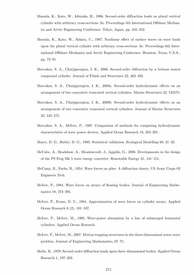
Masuda, K., Kato, W., Ishizuka, H., 1986. Second-order diffraction loads on plural vertical
cylinder with arbitrary cross-sections. In: Proceedings 5th International Offshore Mechan-
ics and Arctic Engineering Conference. Tokyo, Japan, pp. 345–352.
Masuda, K., Kato, W., Sakata, C., 1987. Nonlinear effect of surface waves on wave loads
upon the plural vertical cylinder with arbitrary cross-sections. In: Proceedings 6th Inter-
national Offshore Mechanics and Arctic Engineering Conference. Houston, Texas, U.S.A.,
pp. 72–81.
Mavrakos, S. A., Chatjigeorgiou, I. K., 2006. Second-order diffraction by a bottom seated
compound cylinder. Journal of Fluids and Structures 22, 463–492.
Mavrakos, S. A., Chatjigeorgiou, I. K., 2009a. Second-order hydrodynamic effects on an
arrangement of two concentric truncated vertical cylinders. Marine Structures 22, 545575.
Mavrakos, S. A., Chatjigeorgiou, I. K., 2009b. Second-order hydrodynamic effects on an
arrangement of two concentric truncated vertical cylinders. Journal of Marine Structures
22, 545–575.
Mavrakos, S. A., McIver, P., 1997. Comparison of methods for computing hydrodynamic
characteristics of wave power devices. Applied Ocean Research 19, 283–291.
Mayer, D. G., Butler, D. G., 1993. Statistical validation. Ecological Modelling 68, 21–32.
McCabe, A., Bradshaw, A., Meadowcroft, J., Aggidis, G., 2006. Developments in the design
of the PS Frog Mk 5 wave energy converter. Renewable Energy 31, 141–151.
McCamy, R., Fuchs, R., 1954. Wave forces on piles: A diffraction theory. US Army Corps Of
Engineers Tech.
McIver, P., 1984. Wave forces on arrays of floating bodies. Journal of Engineering Mathe-
matics 18, 273–285.
McIver, P., Evans, D. V., 1984. Approximation of wave forces on cylinder arrays. Applied
Ocean Research 6 (2), 101–107.
McIver, P., McIver, M., 1995. Wave-power absorption by a line of submerged horizontal
cylinders. Applied Ocean Research.
McIver, P., McIver, M., 2007. Motion trapping structures in the three-dimensional water-wave
problem. Journal of Engineering Mathematics, 67–75.
Molin, B., 1979. Second-order diffraction loads upon three dimensional bodies. Applied Ocean
Research 1, 197–202.
211
Newman, J. N., 1990a. Second-harmonic wave diffraction at large depths. Journal of Fluid
Mechanics 213, 59–70.
Newman, J. N., 1990b. The second-order wave force on a vertical cylinder. Journal of Fluid
Mechanics 320, 417–443.
Newman, J. N., 2001. Wave effects on multiple bodies. Hydrodynamics in Ship and Ocean
Engineering, 326.
Ocean Navitas Ltd, March 2011. Official website for Aegir Dynamo wave energy converter.
URL http://www.oceannavitas.com/index.html
Ocean Power Technologies Inc, March 2011. Official website for PowerBuoy wave energy
converter.
URL http://www.oceanpowertechnologies.com
OceanEnergy Ltd, May 2011. Official website for OE Buoy.
Ohl, C. O. G., Eatock Taylor, P. H., Taylor, P. H., Borthwick, A. G., 2001. Water wave
diffraction by a cylinder array. part 1. regular waves. Journal of the Society Of Naval
Architects Of Japan 442, 1 – 32.
Pelamis Wave Power Ltd, March 2011. Official website for Pelamis wave energy converter.
URL http://www.pelamiswave.com/
Prado, M. G. S., Gardner, F., Damen, M., Polinder, H., 2006. Modelling and test results of
the archimedes wave swing. Proceedings of Institute of Mechanical Engineers 220.
Rahm, M., 2010. Ocean wave energy: Underwater substation system for wave energy con-
verters. Ph.D. thesis, Uppsala University, Disciplinary Domain of Science and Technology,
Technology, Department of Engineering Sciences, Electricity.
REN21, 2010. Renewables 2010 global status report. Tech. rep., Renewable Energy Policy
Network for the 21st Century.
Salcedo, F., Ruiz-Minguela, P., Rodriguez, R., Ricci, P., Santos, M., 2009. Oceantec: Sea
trials of a quarter scale prototype. In: Proceedings of the 8th European Wave and Tidal
Energy Conference. Uppsala, Sweden, 2009, pp. 460–465.
Salkind, N. J., 2010. Encyclopedia of Research Design. SAGE Publications, Inc.
Salter, S. H., 1982. The use of gyros as a reference frame. In: Proceedings of the Second
International Symposium on Wave Energy Utilization. pp. 99–115.
212
Salter, S. H., Taylor, J. R. M., Caldwell, N. J., 2002. Power conversion mechanisms for wave
energy. In: Proceedings of the Institute of Mechanical Engineers. Vol. 216. pp. 1–27.
Sarpkaya, T., Isaacson, M., 1981. Mechanics of Wave Forces on Offshore Structures. Van
Nostrand Reinhold Company, New York.
Shifler, D. A., 2005. Understanding material interactions in marine environments to promote
extended structural life. Corrosion Science 47 (10), 2335–2352.
Simon, M. J., 1982. Multiple scattering in arrays of axisymmetric wave-energy devices. part
1. a matrix method using a plane-wave approximation. Journal of Fluid Mechanics 120,
1–25.
Stallard, T., Stansby, P. K., Weller, S. D., Williamson, A. C., 2009a. Float design to limit
displacement in severe seas. In: Proceedings of the 8th European Wave and Tidal Energy
Conference. pp. 601–609.
Stallard, T., Stansby, P. K., Williamson, A., July 2008. An experimental study of closely
spaced point absorber arrays. In: Proceedings of the Eighteenth International Offshore
and Polar Engineering Conference. Vancouver, BC, Canada, pp. 417–424.
Stallard, T. J., Weller, S. D., Stansby, P., 2009b. Limiting heave response of a wave energy
device by draft adjustment with upper surface tension. Applied Ocean Research, 282–289.
Stokes, G. G., 1846. Report on recent researches in hydrodynamics. British Association for
the Advancement of Science Report.
Sustainable Economically Efficient Wave Energy Converter Project, March 2011. Official
website for FO3 wave energy converter.
URL http://www.seewec.org/index.html
Swan, C., Taylor, P. H., Van Langen, H., 1997. Observations of wave-structure interaction
for a multi-legged concrete platform. Applied Ocean Research 19, 309–327.
Taghipour, R., Moan, T., 2008. Efficient frequency-domain analysis of dynamic response for
the multi-body wave energy converter in multi-directional waves. In: Proceedings of the
Eighteenth (2008) International Offshore and Polar Engineering Conference. pp. 357–365.
Tedd, J., Kofoeda, J. P., 2009. Measurements of overtopping flow time series on the Wave
Dragon wave energy converter. Renewable Energy 34 (3), 711–717.
The University of Manchester, March 2011. Official website for Manchester Bobber wave
energy converter.
URL http://www.manchesterbobber.com
213
Thomas, G. P., Evans, D. V., 1981. Arrays of three-dimensional wave-energy absorbers.
Journal of Fluid Mechanics 108, 67 – 88.
Thomas, S. T., Weller, S., Stallard, T., 2008. Float response within an array: Numerical and
experimental comparison. In: Proceedings of the 2nd International Conference on Ocean
Energy.
Uppsala Univeritat, March 2011. Wave power project - Lysekil.
URL http://www.el.angstrom.uu.se/forskningsprojekt/WavePower/
Lysekilsprojektet_E.html
Ursell, F., 1987. Mathematical aspects of trapping modes in the theory of surface waves.
Journal of Fluid Mechanics 183, 421–437.
Vantorre, M., Banasiak, R., Verhoeven, R., 2004. Modelling of hydraulic performance and
wave energy extraction by a point absorber in heave. Applied Ocean Research 26 (1-2), 61
– 72.
URL http://www.sciencedirect.com/science/article/pii/S0141118704000392
Vicinanza, D., Frigaard, P., 2008. Wave pressure acting on a seawave slot-cone generator.
Coastal Engineering 55 (6), 553–568.
Wacher, A., Neilsen, K., 2010. Mathematical and numerical modeling of the aquabuoy wave
energy converter. Mathematics-in-Industry Case Studies Journal.
WAMIT, Inc, 2008. WAMIT User Manual. WAMIT, Inc.
Washio, Y., Osawa, H., Nagata, Y., Fujii, F., Furuyama, H., Fujita, T., 2000. The offshore
floating type wave power device “Mighty Whale”: Open sea tests. In: Proceedings of the
Tenth International Offshore and Polar Engineering Conference. pp. 373–380.
Wave Star A/S, March 2011. Official website for Wave Star wave energy converter.
URL http://wavestarenergy.com/
Wavebob Ltd, March 2011. Official website for Wavebob wave energy converter.
URL http://www.wavebob.com/
Weber, J., Mouwen, F., Parish, A., Robertson, D., 2009. Wavebob - research and develop-
ment network and tools in the context of systems engineering. In: Proceedings of the 8th
European Wave and Tidal Energy Conference. Uppsala, Sweden, 2009, pp. 416–420.
Wehausen, J. V., Laitone, E. V., 1960. Surface waves. Handbuch der Physik 9, 446–778.
214
Weller, S., 2009. Experimental measurements of irregular wave interaction factors in closely
spaced arrays. In: Proceedings of the 8th European Wave and Tidal Energy Conference.
pp. 952–960.
Weller, S. D., 2010. Wave energy extraction from device arrays: Experimental investigation
in a large wave facility. Ph.D. thesis, University of Manchester.
Whittaker, T., Collier, D., Folley, M., Osterried, M., Henry, A., Crowley, M., 2007. The
development of Oyster - a shallow water surging wave energy converter. In: Proceedings
of 7th European Wave Tidal Energy Conference.
Williams, A. N., Demirbilek, Z., 1988. Hydrodynamic interactions in floating cylinder arrays
- I. wave scattering. Ocean Engineering 15 (6), 549 – 583.
Woodroffe, C. D., 2002. Coasts: Form, Process and Evolution. Cambridge University Press.
215