investigations of spnd noise signals in vver-440 …spn detectors is studied through models. 1...

International ConferenceNuclear Energy in Central Europe 2001Hoteli Bernardin, Portorož, Slovenia, September 10-13, 2001www: http://www.drustvo-js.si/port2001/ e-mail:[email protected].:+ 386 1 588 5247, + 386 1 588 5311 fax:+ 386 1 561 2335Nuclear Society of Slovenia, PORT2001, Jamova 39, SI-1000 Ljubljana, Slovenia

510.1

INVESTIGATIONS OF SPND NOISE SIGNALSIN VVER-440 REACTORS

S. Kiss, S. Lipcsei and G. Házi*

KFKI-Atomic Energy Research InstituteApplied Reactor Physics Department

* Simulator DepartmentH–1525 Budapest 114, P.O. Box 49, Hungary

[email protected], [email protected], [email protected]

ABSTRACT

This paper describes and characterises SPND noise measurements of an operatingVVER-440 nuclear reactor. Characteristics of the signal can be radically influenced by thegeometrical properties of the detector and the cable and by the measuring arrangement.Structure of phase spectra showing propagating perturbations measured on uncompensatedSPN detectors is studied through models.

1 INTRODUCTION

One of the features of reactor noise diagnostics – being also a difficulty – is that theprocedure of investigation is mainly based on the operational detectors (ionization chambers,self powered neutron detectors, thermocouples etc.) of the reactor instrumentation, becausethe extreme conditions – high temperature and intensive radiation – dominating inside thereactor can be permanently stood by specially built detectors. The main disadvantage of usingoperational detectors is that they are designed to measure slow, steady-state processes, thustheir frequency response is not optimal to measure fluctuating signals. Generally there are nocalibration or transfer characteristics presented for the frequency range used in noisediagnostics applications i.e. measurement and analysis of fluctuating signals. Although theproblems coming from these lacks can be solved, possibilities and results of the quantitativeanalysis are made worse and more difficult.

One of the most important devices used in the diagnosis of the reactor core is in-coreneutron detector. Knowledge of transfer characteristics of the sensors and on the measurementprocess is essential for the analysis of the noise signals and other quantities calculated fromthe noise signals. For example the current produced by the cable of neutron detectors is addedto the detector signal and it may significantly modify the characteristics of the measuredsignal. Signal characteristics can be radically influenced by the geometrical properties of thedetector and the cable and by the measuring arrangement. Uncompensated neutron detectorsused in VVER 440 type reactors are investigated in Chapter 2 for studying dynamiccharacteristics of the detectors. It is demonstrated by measurement data that the currentproduced inside the cable significantly influences the characteristics of the fluctuating signals.

Dynamic behavior of the detectors is investigated through measurements; theoreticalaspects of the measurement of propagating perturbations are discussed in Chapter 3.

mailto:[email protected]



510.2

Proceedings of the International Conference Nuclear Energy in Central Europe, Portorož, Slovenia, Sept. 10-13, 2001

Model experiments and simulations are made for determining the velocity ofpropagating perturbations. Experiments with the noise simulator are summarized in Chapter4.

Experiences gained from simulation are used to make real measurements better; theyare used to decrease the deviation of the velocity estimation. Results of the experimentscarried out with real measurements are included in Chapter 5.

2 PROPERTIES OF THE IN-CORE NEUTRON DETECTORS (SPND STRINGS)

In Paks VVER 440 type reactors the measurement of the neutron flux is carried out withusing 36 strings of neutron detectors. Each string is placed in the central tube of fuelassemblies. Arrangement of the fuel assemblies containing detector string is approximatelyequidistant. Each detector string consists of seven neutron detectors and the so-calledcompensation cable. The length of the detectors is 20 cm and their center is placed at 30.5 cmfrom each other (Fig. 1).

N1 N2 N3 N4 N5 N6 N7 compensation cable

reactor core

20 20 10.5

202

20 10.5 20 10.5 20 10.5 20 10.5 20 10.5 20 19

242

detector

coolant

Figure 1: Arrangement of an SPN detector string (lengths are given in centimeters)

Length of the compensation cable corresponds to the longest cable length in the string(this is the cable of the detector at the lowest level). In the Paks reactors there are SPN (SelfPowered Neutron or β-emitter neutron) detectors with rhodium emitter. There are no factorydata about the dynamic features of the rhodium detector (e.g. its frequency response, which isimportant for noise diagnostics).

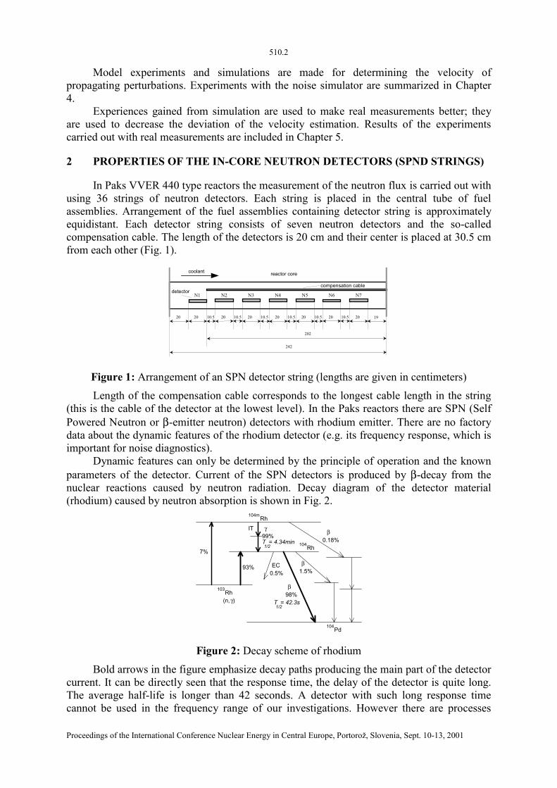
Dynamic features can only be determined by the principle of operation and the knownparameters of the detector. Current of the SPN detectors is produced by β-decay from thenuclear reactions caused by neutron radiation. Decay diagram of the detector material(rhodium) caused by neutron absorption is shown in Fig. 2.

Rh103

(n, )

7%

Pd104

Rh104m

93%

Rh104

β

γ

γ98%

99%

EC0.5%

β1.5%

β0.18%

T = 42.3s1/2

T = 4.34min1/2

IT

Figure 2: Decay scheme of rhodium

Bold arrows in the figure emphasize decay paths producing the main part of the detectorcurrent. It can be directly seen that the response time, the delay of the detector is quite long.The average half-life is longer than 42 seconds. A detector with such long response timecannot be used in the frequency range of our investigations. However there are processes

510.3


producing so called prompt electrons in the material of the detector in addition to nuclearreactions shown in the figure. After the nuclear reaction the material of the detector is reachedby intensive γ-radiation producing free electrons due to photo-effect and pair production. Apart of electrons produced (before recombination) reaches the electrodes and produces ions inthe detector. The amount of the current produced mainly depends on the construction andmaterials of the detector. The ratio of the prompt signal is given by the manufacturer of thedetector as the percent of the steady state signal measured by the detector. This ratio is about6–10 % depending on the production technology, the thickness of the emitter and the aging ofthe detector. In the case of Russian made rhodium SPN detectors the ratio is approximately7 %. The amount of the rhodium in the detector decreases gradually due to the radiation.During a fuel cycle this decreasing can reach even 10–15 % depending on the neutron fluencereaching the detector. Thus detectors must be periodically calibrated and they must bereplaced in every 3–4 years. It can be seen from a simple calculation that the level of thesignal part coming from the delayed neutrons goes under the 7 % of the whole signal at 0.015Hz, thus the spectra used for noise diagnostics evaluations practically contain only the promptresponse of the detector. (The spectra generally used during noise analysis have 50 Hzfrequency range and 512 spectrum lines, thus the first line is at 0.098 Hz.)

Knowing the decay diagram and the prompt ratio, response function of the detectorcould be given quite well. Nevertheless the dependence of the prompt ratio on time is notexactly known. There were and are several suggestions to make the response time of thedetector better, both in theoretical and practical ways [1, 2, 3]. Unfortunately none of them issufficient to reach the speed needed for noise diagnostic measurements.

There is an important aspect rarely mentioned in papers on neutron detectors. Duringthe detection there is a difficulty, the so-called cable effect, i.e. some current is also producedin the cable of the detector distorting the result of the measurement. There are several ways toeliminate the cable effect. In Fig. 3, in addition to the basic circuit diagram of neutrondetectors, there are three solutions shown as typical ways for the compensation of the cableeffect. In the most enhanced solution a double wired cable is used. One of the wires isattached normally to the detector and the signal produced on the other (so calledcompensation) wire is subtracted from the signal coming from the detector. Because thematerial and the path of the compensation wire is identical to the wire used to attach thedetector, thus the subtraction is the most accurate way to neglect the noises added to thesignal of the detector. Unfortunately the detector mounted with compensation cable is moresensitive to damages and its manufacturing is more difficult, thus uncompensated detectorsare still frequently used. This is the situation in Paks, as well, and the distorting effect of thesignal cable is taken into consideration through calculations. There is an additional cable (aso-called compensation cable) inserted along with each detector string, where the length ofthis cable is identical to the cable of the detector at the lowest position. The amount of thecurrent measured on the compensation cable is used in the calculation to restore the detectorsignal: for the lowest detector the whole amount is used, for the other detectors the ratio of thelength of the cables and the shape of the neutron flux is taken into consideration.

At Paks the currents measured on the detectors and on the compensation cable haveopposite directions to each other and recently the current measured on the compensation cablehas been about 6–8 % of the current of the mid level detectors.

As the new detectors gradually changed the old ones, this ratio has decreased to its halfor third since the end of the 80's. The currents measured on the old detectors compared to thenew ones have decreased to their 70 % on the average, while cable currents have decreased totheir 30 %. Currents measured on the detectors and compensation cables before the change ofthe production technology of the detectors are listed in Fig. 4, and after this change in Fig. 5.Data are taken from the archives of the Paks core monitoring system called VERONA [4, 5].

510.4


R

R

v

R v

.

. .

Arrangem ent of a com pensated SPN detector

Uncom pensated SPN detector

R hodium em itter

Isolating m aterial

C ladding and collector

C om pensation cable

Shielded cable

signal cable

Shielding

Resistor

R

R

v

.

.

SPN detector with external com pensation cable and extended signal cable

.


R

R

v

.

.

SPN detector with external com pensation cable

.


"Live tail"

Figure 3: Circuit block diagrams for the SPN detectors

Figure 4: Currents of the old type in-core neutron detectors and compensation cables inUnit 4 of Paks NPP. Cable currents are placed in the fields marked with K.

The amount of the cable current depends on the quantity and the ratio of thecomponents and trace elements in the material of the detector. This quantity and ratio can besignificantly changed as a function of the neutron fluence and the cross section of the givenisotope. A hardly traceable change of the cable current is caused by these changes. (Thisphenomenon was also observed on the SPND strings at Paks insomuch that there weresometimes positive currents measured on the very new SPND strings, however their value is

510.5


definitely smaller than the absolute value of the negative current measured on the cablesduring normal operation. Anyway all the currents measured on cables come to stay atnegative value after some month of operation [6, 7].) It was noticed by investigatingVERONA archive data that the current measured on different cables may significantly differfrom each other, even if they were used under similar operating conditions. See e.g. the dataof the three similar detector strings with significantly different cable current in Table 1.Studying the sum charge provided by the detectors one can conclude that the detectors spendtheir third cycle in the reactor. The difference between the sum charges at the same detectorlevels is less than 15 %. Detector currents normalized with the burn-out (describing the shapeof the neutron flux) are also in a 15 % range. The first two detector strings are placed in newfuel assemblies while the third is in an assembly spending its second fuel cycle in the reactor.The above differences cannot cause such large differences in the currents on the cables. Thedifferences between the cable currents can also be observed on detector strings in their firstand second fuel cycle. In the detector strings used in the 80's there were three times largercable currents measured in absolute value (Fig. 6). In the graphs of Fig. 6 the empiricaldistribution of the currents measured on the compensation cables are shown as the percent ofthe detector currents in the same string (the graphs from left to right were made from data ofthe first fuel cycle of Unit 4 in 1987 and of the 14th cycle of Unit 2 in 1997, respectively).The graphs show clearly that the cable current of the detectors used in the 80's wassignificantly (approximately three times) larger than of the new ones. The relatively largevalue between 0.41 % and 2.61 % of the first graph indicates that the new type detectors weregoing to be applied in that period.

Figure 5: Currents of the new type in-core neutron detectors and compensation cables in Unit4 of Paks NPP. Cable currents are placed in the fields marked with K.

In point of view of noise diagnostics cable current has a special interest because theprompt current of the detector and the cable current appear together in the noise signals. In anextreme case (with the detectors used in the 80's) at certain frequencies the absolute value ofthe contribution from the cable current may exceed the prompt response of the detector for thedetectors with the longest cable. To demonstrate this behavior a measurement was chosenfrom the 80's, its data are summarized in Table 2.

510.6


VERONA archive detector data, 14.10.1997, Unit 2, Cycle 14Coord. of detectorstring 17-58

Level of the detector 1 2 3 4 5 6 7 CableMeasured current [µA] 0.53 0.66 0.71 0.71 0.67 0.59 0.45 -0.0028Current normalized ondetector burn-out [µA] 0.82 1.08 1.18 1.12 1.01 0.85 0.54

Average linear powerrate [MW/m] 1.87 2.21 2.34 2.21 1.96 1.57 0.97

Accumulated detectorcurrent [mA min] 1301.3 1538.4 1645.6 1597.4 1556.3 1493.6 1178.0

Coord. of detectorstring 08-27




Coord. of detectorstring 18-51




Table 1: Detector and cable currents extracted from archive data of VERONA coremonitoring system.

Unit 4, Cycle 1 - 06.10.1987

0

2

4

6

8

10

12

0,41% 2,61% 4,81% 7,00% 9,20% 11,40% 13,60% 15,80%

Unit 2, Cycle 14 - 14.10.1997

0

2

4

6

8

10

12

0,45% 1,22% 1,98% 2,75% 3,52% 4,28% 5,05% 5,82%

Figure 6: Empirical distribution of the current of the compensation cable expressed as thepercent of the detector current averaged along the string.

Noise diagnostic measurement, 12.11.1987, Unit 3, Cycle 1Coord. of detector string 13-40Detector level N1 N2 N3 N4 N5 N6 N7 N8 N1-N8Measured DC [µA] 0.98 1.13 - 1.19 1.14 1.07 0.19 -0.09 0.89Noise RMS [10-3·µA] 4.5 5.8 - 10.8 13.0 19.1 3.4 12.4 7.9Phase between the detectorand the cable in the range 0-5Hz [deg]

< |90| < |160| - >|150| >|150| >|150| >|150| 0 -

Table 2: Measurement data of detector and cable currents.

510.7


In Table 2 N8 stands for the compensation cable. N1-N8 is the difference between thesignal of the detector N1 and of the compensation cable. (It can be concluded from themeasurement report that detector N3 or its electronics was failed during the measurement.)Phase diagram between the detector signals of the table are shown in Fig. 7. The currentsproduced globally (i.e. identically in each point of the cable and the detector) are counter-phase because the signals have opposite signs. Thus at a given frequency the sign of theresulting signal from the superposition of the detector and cable current is determined by thecurrent which is larger in absolute value. Consequently if at a given frequency the current ofthe compensating cable and of detector N1 are in-phase, then cable current is dominant in theresulting signal measured as N1 (i.e. the absolute value of the cable current is larger than onthe detector), while when they are counter-phase the direction of the resulting signal isdominated by the detector current (i.e. the absolute value of the detector current is larger thanthe cable current).

-180

0

180N2 -N1

Pha

se [d

eg]

-180

0

180N4 -N1

Pha

se [d

eg]

-180

0

180N5 -N1

Pha

se [d

eg]

-180

0

180N6 -N1

Pha

se [d

eg]

-180

0

180N7 -N1

Pha

se [d

eg]

0 5 10-180

0

180N8 -N1

Frequency [Hz]

Pha

se [d

eg]

N4 -N2

N5 -N2

N6 -N2

N7 -N2

0 5 10

N8 -N2

Frequency [Hz]

N5 -N4

N6 -N4

N7 -N4

0 5 10

N8 -N4

Frequency [Hz]

N6 -N5

N7 -N5

0 5 10

N8 -N5

Frequency [Hz]

N7 -N6

0 5 10

N8 -N6

Frequency [Hz]0 5 10

N8 -N7

Frequency [Hz]

Figure 7: Phase diagrams between the detector signals of detector string 13-40.

By the phase data of Table 2 and the phase diagrams of Fig. 7 between cable anddetector signals it can be seen that the current of the cables mounted to detectors N1 and N2exceeds the detector current in the frequency range between 0 and 5 Hz. The larger phasevalue can be seen at detector N2 indicates that although the component from the cable issmaller in the comparison to detector N1, it still exceeds the current of the detector. Counter-phase between the detectors N4...N7 and the compensation cable shows that the cable currentremains smaller than the detector current because of the shorter cable length. That is to say thedetector current and the cable current are equalized in the range between detectors N2 and N4.From the RMS values one can see that RMS of the cable signal in absolute value is largeenough to exceed detector currents in case of the first two detectors. Subtracting the time

510.8


series of the cable from the time series of detector N1 gives the undistorted time series of thedetector. Based on the subtraction we got that the RMS of the signal of the detector is the 64% of the RMS of the signal on its cable. In Fig. 8 the APSDs of the signal of the cable (N8)and the detector (N1) and the compensated signal of the detector (N1-N8) are shown in thesame coordinate system.

0 0.5 1 1.5 2 2.5 3 0

20

40

60

80

100

120

Frequency [Hz]

APSD [nA2/s]

13-40/N1 13-40/N8 13-40/N1 -13-40/N8

Figure 8: APSD of the current of the cable (N8) and the detector (N1) and of thecompensated current of the detector (N1-N8).

Fig. 8 shows that in the lower frequency range the real (compensated) current (N1-N8)of the detector is smaller than the current of cable (N8).

3 ESTIMATION OF THE VELOCITY OF THE COOLANT FLOW FROMNEUTRON NOISE SIGNALS

A part of the neutron flux fluctuations, which can be observed in the signals from theneutron detectors is induced by the perturbations in the coolant going through the reactor.Phenomena caused by propagating perturbations are well known in measurement techniquesand noise diagnostics, thus in our model experiments to analyze the effect of the cable currentthe effect of perturbations propagating along detector strings was investigated. Beforeintroducing our investigations, the most important informations are summarized aboutperturbations going through the reactor.

3.1 Investigation of propagating perturbations

Inhomogenities in the coolant flow going through the reactor – such as fluctuation ofthe density, fluctuation in the concentration of boron etc. – cause perturbations in the neutronflux by changing the macroscopic cross sections. Thus a perturbation going in front of adetector appears in the signal of the detector as a small transient with a time delay, whichproportional to the distance between the detectors (Fig. 9).

The velocity of the coolant flow can easily be determined with a simple division usingthe transit time measured between the detectors. Because the velocity of the coolant can onlybe determined with indirect calculations during the reactor operation, so in certain cases itwould be important to have a measurement procedure to determine the velocity of the coolantflow at given positions. There are several ways for the determination of the transit time, e.g.by determining the steepness of linear phase measured between the detector signals or byidentifying the peak characterizing the transit time in the cross correlation function betweenthe signals.

510.9


perturbation velocity of the perturbation

tim e series of the detector signals

d1 d2

)(1 ti

)(2 ti

v

detectors

l

vl=2,1τ

Figure 9: Transit time of the perturbation can be estimated using the time signals of thedetectors

Here is a list of notations used in our forms:

dtetii ti∫∞

∞−

−= ωω )()( is the Fourier transform of a signal )(ti

)()()( 111 ωωω iiAPSD ⋅= is the Auto Power Spectral Densities (or auto spectrum)

)()()( 212,1 ωωω iiCPSD ⋅= is the Cross Power Spectral Densities (or cross spectrum)

K stands for the expected value of …, and ω for the circular frequency and the barfor the complex conjugate.

The equation )()( 2,112 τ−= titi is valid for the time signals of the detector in Fig. 9,

where vl=2,1τ is the transport time between the detectors, l stands for the distance between

them and v denotes the velocity of the propagating perturbation. The Fourier transform of thisequation is 2,1)()( 12

ωτωω ieii −= .Expressing the cross spectrum between the two signals with the auto spectrum of i1

2,12,1111212,1 )()()()( ωτωτωωωω ii eAPSDeiiiiCPSD =⋅=⋅= (1)

and now the linear phase caused by the propagating perturbation is

( ) 2,12,1arg ωτϕ == CPSD , which equals to zero at 2,1τ

ω n= and equals to π at 2

122,1τ

ω += n ,

where n is an arbitrary integer.During the investigation of the perturbation propagating through the reactor a difficulty

is caused by the so called global noise which is also detected by the detector, i.e. not only thepropagating perturbation is seen by the detector but a noise also, which can be sensed at eachpoint of the reactor. That is to say that the detector measures a local and a global noise fieldtogether. (More detailed information can be gained on local-global theorem in [8, 9, 10, 11and 12].) Based on the local-global theorem the signal measured by an in-core neutrondetector can be well separated to a local and a global component:

)t()t()t( gllo iii += .

By a definition of the 70's the global component is generated by the reactivity noisefluctuating in-phase in the whole reactor, while the local component is originated from theaxially propagating perturbations. In the earlier stage of the research the use of the local and

510.10


global terms was unsettled. By the most frequently used definition a perturbation changes theneutron field in its neighborhood, called local component, while all other changes in theneutron field - caused even by other noise sources - are global. Later the idea has slightlychanged and then local and global component were meant the local and global (extensive)changes in the neutron flux caused by one perturbation, i.e. changes are from the same source.

Axially propagating perturbations are bubbles in the coolant in boiling water reactors(BWRs) and coolant parts of different density caused by the changes of the temperature inpressurized water reactors (PWRs). Neutron physical parameters of the coolant are changed inthe neighborhood of these perturbations, and as a consequence neutron flux also changes,which change finally appears in the signal of the in-core neutron detectors as fluctuation.

Linear phase above ~1 Hz observed between in-core neutron detectors in BWRs wasalready earlier regarded as an indication of the presence of the local effect, while thefrequency range below 1 Hz was dominated by an approximately zero phase in accordancewith the global effect [13]. Thorough investigation of the behavior was considered to beimportant, because the velocity of the coolant flow can be estimated from the steep of thelinear phase, in so far it is caused by propagating perturbation.

When the coolant flows upward in the reactor, the signal )t(ui of the upper neutrondetector can be written as

(...))()τt()t( ++−= tiii gllolu ,

where )t( ),t( lol

lou ii are the local components of the neutron noise at the upper and lower

part of the reactor vessel [8]. The first term stands for the process of propagation, while thethird term describes the formation of steam between these two points (the latter term isneglected in PWRs). In the frequency domain:

)()ω()ω( ,iω ωτ gllolu ieii ul += −

=+⋅+=⋅= − ))()(())()(()()( ,, ωωωωωω ωτ glilo

lgllo

lulul ieiiiiiCPSD ul

+⋅+⋅+⋅= ulul ilol

glgllol

ilol

lol eiiiieii ,, )()()()()()( ωτωτ ωωωωωω

=⋅+ )()( ωω glgl ii

=+++= ulul ilogll

gllol

ilol

gl eCPSDCPSDeAPSDAPSD ,, ,

, ωτωτ

ulilol

gl eAPSDAPSD ,ωτ+=

if 0 and 0 ,,

, == ulilogll

gllol eCPSDCPSD ωτ .

Note that the simple equation without global effect (1) can be gained if there is noglobal effect appearing in any of the signals of the detectors:

ululul ilol

ilogll

ilolul eAPSDeCPSDeAPSDCPSD ,,, ,

,ωτωτωτ =+=

I.e. the phase shift between the two points is

)cos(1)sin(

arctg,

,

ul

ul

GG

ωτωτ

ϕ+

= , where gl

lol

APSDAPSDG = .

510.11


The above expression of phase describes well the shape of the phase portraits or at leasttheir certain regions [14, 16, 17]. It is well demonstrated by the expression how the phasediagram is distorted and forced to the zero phases by the global effect. Unfortunately incontrast with the assumptions above the phase portraits measured between the detectors areoften much more complex thus the approximation above cannot be used. In many casessignificant difference was found between the velocities measured in experiments and thevelocities determined by noise diagnostics methods based on the linear phase. (The modelabove is described in more detail in [14, 15, 16, 17, 18 and 19].) The papers on this topic havefrequently described some new source of distortion in the linear phase, but then the knowndistortions were generally neglected. Taking into account all of these effects together inanalytical methods is virtually impossible. All of the effects are taken into account in ournoise simulator experiments, and a new, previously neglected effect is also considered, which– as we prove – can also influence the accuracy of the velocity estimation from the steep ofthe linear phase diagram. Note that other noise diagnostic methods – e.g. velocity estimationwith correlation technique or from impulse response functions – can provide useful results.

3.2 Estimation of the velocity from the correlation

A method of the velocity estimation is based on the fact that the correlation functioncalculated between two detectors has local maximum at the position corresponding to thetransport time. In the analysis of the correlation function difficulties raise because the signalsof the neutron detectors in the core of the reactor are highly correlated due to the globalfluctuation. This effect can hide the peak corresponding to the transport time. It is a morefeasible way to use impulse response function calculated between the detector signals whichis less sensible to the global effect, hence the peak characterizing the transport time can bemore easily identified (look at the difference between the upper and lower diagrams ofFig. 10). There is a peak in the diagrams at 0.0 sec due to the global noises (reaching alldetectors at the same time), and another peak on the right, at about 0.4 sec corresponding tothe time delay between the detectors at the 1st and the 5th levels (characterizing the velocityof the perturbations propagating with the coolant flow).

The impulse response function (IMPAB) between the detectors A and B is calculated as

= −

APSDCPSDFFTIMP

A

ABAB

1 ,

where CPSDAB is the cross spectra between the detectors A and B and APSDA is the autospectrum of detector A.

Fluctuations in the signal of the SPN detectors caused by propagating perturbations arequite small in PWRs (0.001–0.01 % of the DC component of the detector signals), while othernoise components can be larger with some orders making the identification of the transportvelocity more difficult. Therefore, where these effects are strong the identification of thevelocity of the perturbations is only possible with large fault, if any. See e.g. the graphs in thethird column of Fig. 10, where the peak at 0.4 sec induced by the propagating perturbation isnear unidentifiable. The diagrams in the center column can be said average, while the firstdiagrams contain especially well identifiable peaks.

510.12


-1 0 15.4

5.6

5.8

6

6.2x 10

-6 04-37/N1-N5

Cro

ss C

orre

latio

n

-1 0 15

5.2

5.4

5.6

5.8

6x 10

-6 17-58/N1-N5

-1 0 1-5

-4

-3

-2

-1

0x 10

-7 15-56/N1-N5

-1 0 1-10

0

10

20

30

4004-37/N1-N5

Impu

lse R

espo

nse

Time [sec]-1 0 1

-10

0

10

20

3017-58/N1-N5

Time [sec]-1 0 1

-10

0

10

20

30

4015-56/N1-N5

Time [sec]

Figure 10: Cross correlation (top) and impulse response (bottom) functions between detectorswith transport time approximately 0.4 sec.

4 MODELS OF THE SPND STRINGS

A model experiment and simulation were performed to clean the process of detectionsof the in-core neutron detectors. First a simplified model was prepared with separated noisecomponents. The main goal with this simplified model was to understand the characteristicsof the different noise components. After the simulation performed on the simplified model, anoise simulator containing a one dimensional reactor model was used as a numericalexperiment. A coupled neutron kinetic and thermo-hydraulic model was applied, which issuitable to model realistically the most important noise propagation processes inside thereactor.

4.1 A simplified model of the SPND strings

A simplified, one-dimensional model was prepared for the measurement of the neutronnoise induced by the perturbations propagating through the reactor (Fig. 11).

The main components of the model are the detector, its cable, the global effect and theperturbation of which measurement is modeled. The measured signal is evolved by thesecomponents altogether.

Perturbation. There are perturbations propagating through the model with size s andvelocity v, and they are characterized by a per-length strength P. In the simplest case thedistribution of the strength of the perturbation can be written as

+≤≤

=otherwise,0

if,),(

svtxvtPtxp ,

where x is the spatial coordinate and t is the time. Using the model a number ofperturbations (enough to make good statistics) was generated, where the parameters s and Pwere generated randomly.

Model of the detector. In the one-dimensional model the detector was substituted with aline of length ld and its center was placed at the position xd, and which is characterized with

510.13


Gd prompt detector sensitivity at its each point. (In our model the sensitivity of the detector isset to 1 and all other sensitivity is given relatively to the sensitivity of the detector.)Dependence of the transfer function of the detector on the location is approximated as

+≤≤

=otherwise.,0

if,)( dddd

d

lxxxGxγ

The current )(tid of the detector is proportional to the strength of the perturbation andto the length of the common part of the perturbation and the line substituting the detector, i.e.

.)(),()( ∫∞

∞−

= dxxtxpti dd γ

A d2

A d1

Perturbation

Detectors substituting the global effect

Detector

i 2

Weight factors

i 1

A c2

A d1

Perturbation

i 2

A c1

A d1

i 1

COMPENSATED DETECTOR UNCOMPENSATED DETECTOR

L c1

H r

L d1

x d2

x d1

L d2

x c1

x c2

v v

P

P P

P

v v

x

+

+ + +

+

+

+ +

Detectors substitutingthe cable effect

Figure 11: One-dimensional noise diagnostic models of SPN detectors measuringpropagating perturbations in case of compensated (left) and uncompensated (right) detector.

Model of the cable. From noise diagnostics viewpoint the cable of the detector is also adetector adding a contribution to the signal of the detector that is hardly separable from thedetector signal, if any. In the one-dimensional model the cable is regarded to a detector withthe length cl , one and of which is at the top end of the detector and the other end is at the topof the reactor, hence its transfer function can be written as

++≤≤+

=otherwise.,0

if,)( cddddc

cllxxlxG

xγ

It is important to emphasize that the current of the cable has opposite direction to thecurrent of the detector, i.e. its specific sensitivity 0≤cG . Current of the cable is arbitrarilydivided into three groups. It is said to be large if 09.0≥cG , then it can be larger than the

510.14


current of the detector. It is said to be normal when 03.009.0 ≥> cG and small if cG>03.0 .The current of the detector representing the cable is caused by the same mechanism as it wasdescribed at the model of the detector, i.e.

∫∞

∞−

= dxxtxpti cc )(),()( γ .

The properly signed current of the cable is added to the current of the detector.

Model of the global effect. The global effect of the reactor is also modeled with adetector of length H, where H is the height of the reactor core. In the most simplified case

≤≤

=otherwise.,0

0 if,)(

HxGxg r

r

The effect of the perturbation on the neutron flux – worth of the perturbation – isestimated with a cosines function:

≤≤

=otherwise.,0

0 if,cos)( HxHxGxg r

r

π

In the model the amount of the )(tglΦ global change of the neutron flux in the reactor isgiven by

.)(),()( ∫∞

∞−

=Φ dxxgtxpt rgl

Then the part the global effect appearing in a real detector can be written as

.)()()()()(, ∫∫∞

∞−

∞

∞−

Φ=Φ= dxxtdxxtti dgl

dgl

gld γγ

From this form it can be seen that the global effect is added to the detector signalmultiplied with a constant factor. Formally it can be considered like the current of a detectorwith )(xgr transfer function were added to the signal of the detector through an amplifierwith an amplification factor

.)(∫∞

∞−

= dxxA dd γ

The cable can be considered in a similar way, i.e. the current produced in the cable bythe global effect is

∫∫∞

∞−

∞

∞−

Φ=Φ=Φ= )()()()()()( tAdxxtdxxtti glcc

glc

glglc γγ , where

510.15


.)(∫∞

∞−

= dxxA cc γ

Thus the total current can be measured on the detector in the simplified model is

)()()()()( tititititi glcc

gldd +++=

Sensitivities of the detectors substituting the different effects were normalized to thesensitivity to the real detector.

4.1.1 Investigation of the dependence on the length

Several characteristics of the signal can be estimated from this model. The currentinduced in a detector of length l by a wave running along the detector can be written as

−+−=

+−=+=

=

∫ )cos()cos()cos()sin(),(00

tc

ltcGc

xtcGdxc

xtGtilxl

ωωωω

ωωω

ωωω

where G stands for the specific sensitivity of the detector and c is the velocity of thewave. After transforming the equation:

⋅

+=

⋅

+=

clt

clcGc

ltc

lcGti

2sin

2sin2

2sin

2

2sin2),( ωωω

ω

ωωω

ωω

Produce the power density function of the wave in the way below:

=′

⋅

′+= ∫∞→

t

ttd

clt

cl

tcGi

0

222

222

2sin

2sin4lim)( ωωω

ωω

=

′+−′⋅

⋅=

=′

=′∞→

tt

tt

tc

ltc

lt

cG0

22

22

22sin

41

21

2sin4lim ωω

ωω

ω

+

+−⋅

⋅=

∞→ clt

clt

cl

tcG

t 22sin

41

22sin

41

21

2sin4lim 2

2

22 ω

ωωω

ωω

ω, where

02

2sin2

2sin2

sin414lim 2

2

22 =

+

+⋅

⋅−

∞→ clt

cl

cl

tcG

t

ωωωωωω

.

Finally

⋅=

clcGi2

sin2)( 22

222 ω

ωω

Substituting 2.02 m for the length of the cable, 2.42 m for the height of the reactor core0.2 m for the length of the detector and 3.2 m/s for the velocity of the coolant flow the curvesof Fig. 12 are obtained.

510.16


0

0.005

0.01

0.015

0.02

0.5 1 1.5 2 2.5 3 3.5 4 4.5 5

[Magnitude]

Frequency [Hz]

Cable Global Detector

⋅=

clcGvi πν

νπ2

22

222 sin

2)(

Figure 12: Shape of the power density function of the cable due to perturbations propagatingalong the cable.

Sensitivities were assumed as 1=dG for the detector, 09.0=cG for the cable and075.0=rG for the global effect. It can be observed that the frequency response steeply

decreases in inverse ratio to the frequency and it is equal to zero at

( ),...2,1 , == nl

ncν

depending on the length of the detector. The limes in the calculation of the powerdensity function in Section 4.1.1 can only be estimated in numerical simulation and in theevaluation of measurements, consequently with final length of the evaluation at low

frequencies the final formula is not valid

>> 3

2

ωct . In practice this means that for

propagating perturbations the effect of the cable disappears above 1 Hz. The length of thedetector modeling the global effect is longer than the length of the cable only with 20 %, thusits APSD do not differs significantly from the APSD of the signal on the cable. Because of theshort size of the real detector the first zero point of its power density function is about 50 Hz.For perturbations propagating perpendicularly to the detector, its frequency response does notchange. In our case it is regarded to linear above 0.1 Hz.

Due to the arrangement of the detector the global noise of the reactor – which means notonly the noise induced by the propagating perturbations – is subtracted from the current of thedetector by the cable (because of its opposite sign). Consequently the longest detector cable ata given specific sensitivity may virtually make the global effect disappeared (if the differencebetween the frequency responses is neglected). Thus the characteristic of the linear phase maybecome significantly better. However in case of too large current of the cable“overcompensation” may occur, which forces the phase portrait to π. This gives the idea, thatthe current of the compensation cable with an appropriate weighting factor can be used tocompensate the global effect.

Testing of how the model works was performed by reproducing the signals of the noisediagnostics measurements made in 1986 on uncompensated detectors with large cable current.Turning back of the phase induced by the cable in the range of 0.5–2 Hz can be well observed(see the curve with dashed line in Fig. 13). Modeling was made through the production of thesignals of detectors N1 and N3 in Fig. 1. The global effect was modeled with a cosine shapedtransfer function. Real measurement results were well reproduced by this quite simple model

510.17


(after setting the specific detector sensitivities in an experimental way). Phase diagramcalculated from the simulation is drawn with solid line in Fig. 13. From the comparison of thephase diagrams one can see that the phase portrait made from the simulated data well matchesto the real measurement.

-150

-100

-50

0

50

100

150

2 4 6 8 10 12

Phase [deg]

Frequency [Hz]

"Simulated" "N1-N3

0

Figure 13: Simulated (solid line) and measured (dashed line) phase between detectors N1 andN3 of detector string 15-32

In spite of the good result the simplified model has an important disadvantage, it doesnot contain thermo-hydraulic and neutron kinetic behavior of the reactor, thus it cannotprovide proper result under 0.5 Hz. A further disadvantage is that there was no globalbackground noise – a noise raising at each point of the reactor independently from theperturbation modeled – added to the model, thus the resulting phase diagram is smoother thanfrom the real measurement. On the other hand this would mean an additional (third)parameter in the model. In a three-dimension model the ratio of the global and localcomponents of a perturbation may definitely larger in the signal of the detector compared tothe one-dimensional model, because the effect of the perturbations in the surrounding fuelassemblies can appear. That is the local component of the perturbation acts in a smalleramount comparing to the global component, because of the longer distance. Thus for the onedimension model the global effect must be taken into consideration with a larger weight. Amore realistic investigation can be performed with the use of the noise simulator containingone dimension reactor model.

4.2 Noise simulation based on one dimension reactor model

For simulation of the signal of SPNDs, a coupled thermohydraulics and neutron kineticsmodel is used. In our simulations we used inlet temperature noise as a driven source. Thenoise was generated as time function by a well-tested random number generator. The dynamicbehaviour of the reactor core is modeled by one-dimensional two-group diffusion equationscoupled with a simple axial model for fuel and coolant. For coupling we used a suitablecorrelation between the group and the thermohydraulics parameters. The equations of themodel are solved by numerical methods and the resulting time series of neutron fluxes areconsidered as virtual measurements. Neutron detectors can be placed anywhere in the reactorcore axially and they measure the thermal neutron flux in the neighbourhood of a givenposition corresponding to the defined length of detector. Although cables of detectors are notmodelled directly in the system, but one can model their effect by associating detectors and asuitable weighting factor with them. The virtual time series are processed by usual signalprocessing techniques as well as real measurements.

Since we model the mechanism of noise propagation, the numerical methods and theirparameters have to be selected carefully. By the means of numerical analysis we could provethat the numerical noise does not influence significantly the physical one. The reader can findmore information about the simulator in [20].

510.18


In the simulator, the signals of the detectors N1 and N3 correspond to the detectors usedin the simple model. In the simulator different values of the specific sensitivity of the cablewere studied in the range of 0.02-0.25. (The specific sensitivity of the detector was unity.)Phase diagrams calculated by the simulator data are displayed in Fig. 14. The graph at the topshows those phase portraits where the absolute value of the cable current was smaller than thecurrent of the detectors, but the global effect was not overcompensated by the cable. Thefigure shows clearly: the phase portrait gains the linear phase shape gradually with theincrease of the specific sensitivity G of the cable (and increasing the sensitivity, the current ofthe cable is also increasing).

-180

-135

-90

-45

0

45

90

135

180

0,0 1,0 2,0 3,0 4,0 5,0 6,0 7,0 8,0 9,0 10,0 11,0 12,0 13,0 14,0 15,0

Frequency [Hz]

Phas

e [d

eg]

G = 0.020

G = 0.060

G = 0.080

G = 0.090

G = 0.100

G = 0.110

-180

-135

-90

-45

0

45

90

135

180

0,0 1,0 2,0 3,0 4,0 5,0 6,0 7,0 8,0 9,0 10,0 11,0 12,0 13,0 14,0 15,0

Frequency [Hz]

Phas

e [d

eg]

G = 0.110

G = 0.120

G = 0.135

G = 0.150

G = 0.175

G = 0.200

G = 0.250

Figure 14: The effect of the cable current on the shape of the phase portraits.

One can see in the bottom picture of Fig. 14, that the phase gradually turns into counter-phase when the sensitivity of the cable reaches its optimum in the compensation of the globaleffect. In this range one of the detectors is overcompensated while the other is not. When bothdetectors are strongly overcompensated, then the characteristics of the phase portrait betweentheir signals becomes similar to the characteristics of the phase portrait between longoverlapped detectors. These features observed in the results of the simulation can be identifiedin the phase portraits of Fig. 7. Accordingly phase portrait characterizing small cable currentcan be seen between the detectors N5 and N6, the global effect is optimally compensatedfrom the phase between N4 and N5, and the characteristics of the overcompensated detectors(when the cable current is larger then the detector current) can be observed in the phaseportrait between N2 and N4.

Based on the results of the simulation we can state that depending on the amount of thecable current, significant differences may occur between the characteristics of the signals ofdetectors in the same conditions. Thus the signal measured on the compensation cable alwaysmust be taken into consideration during the measurements. In the following section theseresults are applied on real measurement data.

510.19


5 CORRECTION OF MEASURED NOISE DIAGNOSTICS TIME SERIES

It was concluded by the simulation that in a certain range the cable current might correctthe shape of the linear phase between the signals of the detectors. Thus if the ratio of thecurrent of the cable and the detector could be controlled in such a way that the globalcomponent of the reactor noise would be considerably decreased by the cable current, or in anideal case it would be totally compensated, then the resulting signals would be more suitableto use in the determination of the velocity.

For the experiments measurement data described in Table 2 were used. Phase diagramsfrom the measurements are displayed in Fig. 7. Compensation of the detector signals wasperformed in such a way that the signal of the compensation cable with a suitable weightingfactor was added to the measured signals. Weighting factors were experimentally determinedwith the cable length of the detectors and the level of the DC signal taken into account tooptimize the linear phase. The applied factors are listed in Table 3. (These factors are uniquefor each detector string.)

Unit 3, Cycle 1, 12.11.1987, measurement 4A, detector string 13-40Detector N1 N2 N3 N4 N5 N6 N7Weighting factor -0.52 -0.25 - 0.28 0.4 0.55 0.16

Table 3: Factors used for compensation of the detector signals.

-180

0

180N2 -N1*

Pha

se [d

eg]

-180

0

180N4 -N1*

Pha

se [d

eg]

-180

0

180N5 -N1*

Pha

se [d

eg]

0 5 10-180

0

180N6 -N1*

Frequency [Hz]

Pha

se [d

eg]

N4 -N2*

N5 -N2*

0 5 10

N6 -N2*

Frequency [Hz]

N5 -N4*

0 5 10

N6 -N4*

Frequency [Hz]0 5 10

N6 -N5*

Frequency [Hz]

Figure 15: Phases between the signals of the detector string with compensation (marked withasterisk) on the first detector only

Phase diagrams in Fig. 15 were calculated between signals where the correction wasapplied on one of the signals of the detector pairs. In the graphs these phases are displayedwith blue lines while the phases of the original signals with green lines. Comparing the two

510.20


kinds of phase portraits one can see that the linearity of the phase diagrams becomesdefinitely better with the change of the cable current. It can be seen that the turning back ofthe phase characterizing the original time series is disappeared in the range 0-3 Hz. The effectof the compensation cable repairing (reconstructing) the phase is the most significant with thedetectors at the lowest levels (where the cable length of the detector is nearly the same as thelength of the compensation cable). For the signals of the detectors at the sixth and seventhlevel (N6 and N7) there is no significant change in the phase diagrams thus phase portraitscreated with detector N7 is not displayed in the figure. This behavior is partly because thehigher the detector level is, the larger amount of compensation would be needed whilecharacteristics of the cable current are more different. (When both signals of the detector pairsare compensated the linearity becomes better below 10 Hz. However, adding the samecomponent to both signals causes in-phase or counter-phase correlation in the higherfrequencies.)

During the compensation of the signals of detectors with low level of cable current thereis now significant change (mainly because of the high signal-to-noise ratio of themeasurement). The effect of the correction in the time series appears not only in the phasediagrams but also in other statistical functions of the signal, e.g. in the correlation functions(Fig. 16).

In Fig. 16 the cross correlation functions (CCFs) between N1 and N7 shown in the leftgraph while N4-N7 is shown in the right graph. The cross correlation functions from theoriginal and the compensated time series are plotted with dash line and solid line,consequently. In the first graph in the range of zero (the range of the global effect) CCF of theoriginal signals has negative values, because of the large cable current of N1 (large meanslarger than the detector signal). The peak at the transport time (0.27 sec) is hardly identifiable.In the CCF between the corrected signals global effect is almost disappeared and the peak atthe transport time can be easily identify.

-1.25 0 1.25-0.25

-0.2

-0.15

-0.1

-0.05

0

0.05

0.1

0.15

0.2

0.25N4* -N1*

Time [sec]-1.25 0 1.25

-0.05

0

0.05

0.1

0.15

0.2N7* -N4*

Time [sec]

Figure 16: Cross correlation functions between the signals of N1 and N4 (left) and N4 andN7 (right) from original (dash line) and compensated (solid line) time series.

Component from the cable current is smaller in the signals of N4 and N7 of the secondgraph comparing to N1. (Cable current of N4 is less than 40 % comparing to N1, N7 is lessthan 5 %.) The global effect is stronger in the CCF of the original signals because of the smallcable current thus the signals in the range of [-1, 1] sec are highly correlated. The peak at thetransport time can at most be suspected in the curve. CCF of the original signals has similarcharacteristics to the CCFs in Fig. 10 with small cable currents. Global effect is highlydecreased in the CCF of the compensated signals and the peak at the transport time hasbecome definite.

510.21


By the experiments made on real time series we can conclude that the simulated data arefit to the measurement results and they prove the effect of the cable current. That is the effectof the cable of uncompensated detector must always be taken into account during processingand analyzing noise diagnostics measurements. It was shown that when detector signals withlarge cable currents are investigated, the results of the processing can be make better using thecurrent of the compensation cable.

6 CONCLUSIONS

Based on the investigations of the signals of uncompensated detectors used inVVER 440 type reactors it was concluded that the currents induced in the cables of thedetectors might differ from each other in a significant amount (it can reach an order ofmagnitude). Cable current – having prompt nature – may influence dynamic behavior of thedetectors, and it appears in the statistical properties of the signals. It can be seen from themeasurements that for the detectors applied in the eighties, the noise diagnosticsmeasurements – using the prompt part of the detector current – cable current exceeded thedetector current in case of the detectors with the longest cables. Thus the influence of thecable current must be taken into consideration for measurements performed byuncompensated detectors.

It was shown with modeling propagating perturbations that cable current has remarkableinfluence on the phase portraits of the signals induced by the propagating perturbations. It wasalso shown that the cable current – because of its opposite direction – compensate the globalfluctuation in the measured signal, thus for certain cable currents linear (or slightly distortedlinear) phase can be measured characterizing propagating perturbations.

Results of the model experiments were checked with calculations made on real signals.Time series of the current of the compensation cable – multiplied with different weightingfactors – were added to the detector signals. With these manipulation characteristics of thepropagating perturbations appeared more clearly in the properties of the modified time series.

7 REFERENCES

[1] H. D. Warren, “Calculation Model for Self-Powered Neutron Detectors”, Nucl. Sci.Eng., 48, 1972, pp. 331-342.

[2] S. V. Guru, D. K. Wehe, “Instantaneous Flux Measurements Using the BackgroundSignal of the Rhodium Self-Powered Neutron Detector”, Ann. Nucl. Energy, 19, 4,1992, pp. 203-215.

[3] K. Kulacsy and I. Lux “A method for prompt calculation of neutron flux from measuredSPND currents”, Ann. Nucl. Energy, 24, 5, 1997, pp. 361-374.

[4] Adorján F., Bürger G., Makai M., Sándor Gy., Valkó J., Végh E., “VERONA – coreevaluation system of Paks NPP”, Mérés és Automatika, 32, 12, 1984 (in Hungarian).

[5] F. Adorján, L. Bürger, I. Lux, M. Makai, J. Valkó, J. Végh, “Core monitoring systemfor VVER-440 PWR’s”, Computerization of Operation and Maintenance for NuclearPower Plants, IAEA-TECDOC-808, 1995.

[6] Adorján F., Végh J., “Investigations based on the VERONA-u archives of Paks NPPUnit 2”, AEKI Research Report, 1994 (in Hungarian).

510.22


[7] Adorján F., Végh J., “Error analysis of the measurements used as input data ofVERONA-u system”, MTA KFKI AEKI Applied Reactor Physics Dept., 1996 (inHungarian).

[8] G. Kosály, “Investigation of the local component of power reactor noise via diffusiontheory”, KFKI Report, KFKI-75-27, 1975.

[9] K. Behringer, G. Kosály, Lj. Kostić, “Theoretical Investigation of the Local and GlobalComponents of the Neutron-Noise Field in a Boiling Water Reactor”, Nucl. Sci. Eng.,63, 1977, pp. 306-318.

[10] G. Kosály, L. Kostic, L. Miteff, G. Váradi, K. Behringer, “Investigation of the localcomponent of the neutron noise in a BWR and its application to the study of two phaseflow”, Prog. Nucl. Energy, 1, 1977, pp. 99.

[11] G. Kosály, R. W. Albrecht, R. D. Crowe, D. J. Dailey, “Neutronic response to twophase flow in a nuclear reactor”, Prog. Nucl. Energy, 9, 1982, pp. 23.

[12] K. Behringer, G. Kosály, I. Pázsit, “Linear Response of the Neutron Field to aPropagating Perturbation of Moderator Density (Two-Group Theory of Boiling WaterReactor Noise”, Nucl. Sci. Eng., 72, 1979, pp. 304-321.

[13] W. Seifritz, F. Cioli, “On-load monitoring of local steam velocity in BWR cores byneutron noise analysis”, Trans. Am. Nucl. Soc., 17, 1973, pp. 451.

[14] T. Katona, L. Meskó, G. Pór, J. Valkó, “Some aspects of the theory of neutron noisedue to propagating perturbances”, Prog. Nucl. Energy, 9, 1982, pp. 209.

[15] F.J. Sweeney, B.R. Upadhyaya, D.J. Shieh, “In-core coolant flow monitoring ofpressurized water reactors using temperature and neutron noise”, Prog. Nucl. Energy,15, 1985, pp. 201.

[16] G. Pór, O. Glöckler, U. Rindelhardt, “Boiling detection in PWRs by noisemeasurement”, Prog. Nucl. Energy, 21, 1988, pp. 555.

[17] J. Valkó, “In-core generated temperature fluctuations and boiling detection inpressurized water reactors”, Ann. Nucl. Energy, 19, 1992, pp. 155.

[18] M. Antonopoulos-Domis , S. Kadi, K. Mourtzanos, “Departure from linearity of neutroncross-spectra phase in BWRs”, Ann. Nucl. Energy, 22, 1995, pp. 39.

[19] M. Antonopoulos-Domis, S. Kadi, “Velocity profile effects on neutron cross-spectra inBWRs”, Ann. Nucl. Energy, 23, 1996, pp. 217.

[20] G. Házi, G. Pór, “Numerical Simulator for Noise Diagnostic Investigations in NPPs”,Ann. Nucl. Energy, 26, 1999, pp. 1113-1130.

investigations of spnd noise signals in vver-440 …spn detectors is studied through models. 1...

Documents