Investor Sophistication andCapital Income Inequality⇤

Marcin KacperczykImperial College London & CEPR

Jaromir NosalBoston College

Luminita StevensUniversity of Maryland

September 28, 2018

Abstract

Capital income inequality is large and growing fast, accounting for a significant por-tion of total income inequality. We study its growth in a general equilibrium portfoliochoice model with endogenous information acquisition and heterogeneity across house-hold sophistication and asset riskiness. The model implies capital income inequalitythat grows with aggregate information technology. Investors di↵erentially adjust boththe size and composition of their portfolios, as unsophisticated investors retrench fromtrading risky securities and shift their portfolios toward safer assets. Technologicalprogress also reduces aggregate returns and increases the volume of transactions, fea-tures that are consistent with recent U.S. data.

⇤We thank Boragan Aruoba, Bruno Biais, Laurent Calvet, John Campbell, Bruce Carlin, John Donaldson,Thierry Foucault, Xavier Gabaix, Mike Golosov, Gita Gopinath, Jungsuk Han, Ron Kaniel, Kai Li, MatteoMaggiori, Gustavo Manso, Alan Moreira, Stijn van Nieuwerburgh, Stavros Panageas, Alexi Savov, JohnShea, Laura Veldkamp, and Venky Venkateswaran for useful suggestions and Joonkyu Choi for researchassistance. Kacperczyk acknowledges research support by a Marie Curie FP7 Integration Grant withinthe 7th European Union Framework Programme and by European Research Council Consolidator Grant.Contact: m.kacperczyk@imperial.ac.uk, jarek.nosal@gmail.com, stevens@econ.umd.edu.

1 Introduction

The rise in income and wealth inequality has been among the most hotly discussed topics in

academic and policy circles.1 Among the possible explanations, heterogeneity in the returns

on savings—due to di↵erences in rates of return or in the composition of the risky portfolio—

has been highlighted as an important driver. This factor has emerged in empirical work on

the wealth distribution, such as Fagereng, Guiso, Malacrino & Pistaferri (2016a; 2016b)

and in research focused on the very top of the wealth distribution (Benhabib, Bisin & Zhu,

2011).2 However, as noted by De Nardi & Fella (2017), more work is needed to understand

the determinants of such heterogeneity.

This paper studies capital income inequality growth in a portfolio choice model with

information constraints. When investors di↵er in their capacity to process news about risky

asset payo↵s, both the size and the composition of the risky portfolios di↵er across investors.

Not surprisingly, this generates inequality. More interestingly, progress in the aggregate

information processing technology can exacerbate this inequality, and this e↵ect can be

economically large, as less sophisticated investors get priced out of high-return assets. This

pecuniary externality arises even in a setting with a single risky asset, but is amplified in an

economy with heterogeneous assets.

At the core of our model is each investor’s decision of how much to invest in assets

with di↵erent risk characteristics. This decision is shaped by the investors’ capacity to pro-

1See Piketty & Saez (2003); Atkinson, Piketty & Saez (2011). A comprehensive discussion is also o↵eredin the 2013 Summer issue of the Journal Economic Perspectives and in Piketty (2014).

2See also the review by Benhabib & Bisin (2017). Saez & Zucman (2016) emphasize the role of dif-ferential savings rates, rather than di↵erential rates of return, in generating wealth inequality. However,their capitalization method imposes homogeneity across investors on the rates of return within asset classes,thereby ruling out one mechanism over the other.

1

cess information about asset payo↵s, and by their choice of how to allocate this capacity

across assets.3 We model the learning choice using the theory of rational inattention of Sims

(2003). While stylized, the framework captures several appealing aspects of learning. First,

getting information about one’s investments requires expending resources. Second, learning

about more volatile assets consumes more resources. Lastly, investors can allocate their in-

formation capacity optimally across di↵erent types of assets, depending on their objective

and the characteristics of the assets they invest in. Our theoretical framework generalizes

existing models—Van Nieuwerburgh & Veldkamp (2010) in particular—by considering het-

erogeneously informed agents investing in multiple heterogeneous assets.4

We analytically characterize three channels of how investor heterogeneity generates cap-

ital income inequality: Investors with higher information capacity hold larger portfolios on

average, tilt their average holdings towards riskier assets within the risky portfolio, and ad-

just their investments more aggressively in response to changes in payo↵s. These patterns are

consistent with the empirical literature on portfolio composition di↵erences between wealthy

and less wealthy investors, going back to Greenwood (1983), and Mankiw & Zeldes (1991),

and discussed more recently by Fagereng et al. (2016b) and Bach, Calvet & Sodini (2015).

Our central result is that growth in aggregate information capacity, interpreted as a gen-

eral progress in information-processing technologies, disproportionately benefits the initially

more skilled investors, and leads to growing capital income inequality. As the aggregate

3In the model, we endow each investor with a particular level of information processing capacity. However,this capacity should be interpreted more broadly, as a stand-in for the individual’s ability to access highquality investment advice, not limited to his or her own knowledge of or ability to invest in financial markets.

4In finance, rational inattention models have been used successfully to address underdiversification puz-zles, price volatility and comovement puzzles, overconfidence, and the home bias, among other applications.References include Peng (2005), Peng & Xiong (2006), Van Nieuwerburgh & Veldkamp (2009; 2010), Mondria(2010). See also Mackowiak & Wiederholt (2009; 2015), Matejka (2015), and Stevens (2018) for applicationsin macroeconomics. Our application to inequality is new, to our knowledge.

2

capacity to process information grows, all investors would like to grow their portfolios. How-

ever, in equilibrium, prices increase in response to the higher demand, and only the sophis-

ticated investors expand their portfolios. The less sophisticated investors are priced out and

retrench to lower-risk, lower-return assets, which amplifies capital income inequality. This

result holds regardless of the learning technology assumed, and the specific functional form

for information acquisition only a↵ects the magnitude of the e↵ect.

Our mechanism is amplified in a setting with heterogeneous assets, because the shifts

in ownership shares occur asymmetrically across assets. Allowing investors to choose how

to learn about di↵erent assets is critical here: With endogenous information choice, the

sophisticated ownership share grows most for the most volatile assets, which are precisely

the assets that generate the largest capital income gains. As a result, the model with multiple

risky assets generates more inequality growth compared with a model with one risky asset.

To provide some guidance regarding the magnitudes of the e↵ects identified in our model,

we conduct a set of numerical experiments in a parameterized economy. We show that a 5%

annual growth in aggregate information capacity5 generates a rise in capital income inequality

of 38% over 24 years. In contrast, an economy with a single risky asset generates only 20%

growth. Calibrating the information capacity growth is challenging because the information

that investors have when they make their investment decisions is not observable. However, for

a range of plausible values of recent growth in information capacity, inequality growth ranges

from 24% to 60%. The corresponding number in the Survey of Consumer Finances (SCF)

for the 1989-2013 period is 87%.6 General progress in information technology also generates

5This annual growth rate is chosen to generate an average market return of 7% in the model. We discussthe parameterization in detail in Section 4.

6We define capital income inequality as the ratio between the average capital income of the top 10%of investors by wealth and that of the bottom 90% of investors by wealth, conditioning on participation in

3

lower market returns, higher market turnover, and larger and more volatile portfolios. These

predictions are broadly consistent with the data on turnover and ownership from CRSP and

Morningstar on stocks and mutual funds over the last 25 years.

Our findings connect to the idea that generating the inequality in outcomes observed in

the data requires linking rates of return to wealth–which is our indicator for access to better

information on investment strategies.7 This idea has a long history, going back to Aiya-

gari (1994), who discusses the wide disparities in portfolio compositions across the wealth

distribution, emphasizing the fact that rich households are much more likely to hold risky

assets. Subsequently, Krusell & Smith (1998) suggest that the data requires that wealthy

agents have higher propensities to save, generate higher returns on savings, or both. Ben-

habib et al. (2011) and Gabaix, Lasry, Lions & Moll (2016) are recent theoretical treatments

and Favilukis (2013), Cao & Luo (2017), and Kasa & Lei (2018) are related quantitative

contributions. We complement this literature along two key dimensions. First, we study the

within-period portfolio problem with multiple risky assets, rather than the dynamic savings

decision with a single risky asset. Second, we study inequality in a general equilibrium con-

text with endogenous returns, rather than with exogenous idiosyncratic investment returns.

Both asset heterogeneity and the endogenous response of asset prices–and hence returns–are

key sources of amplification for inequality.

Our work contributes to a broader literature on inequality in capital income, including the

work on bequests (Cagetti & De Nardi (2006)), limited stock market participation (Guvenen,

2007; 2009), financial literacy (Lusardi, Michaud & Mitchell (2017)), and entrepreneurial tal-

financial markets. The Appendix presents all variable definitions.7This connection is motivated by evidence that has linked trading strategy sophistication to asset prices,

wealth and income levels, such as Calvet, Campbell & Sodini (2009), Chien, Cole & Lustig (2011), andVissing-Jorgensen (2004).

4

ent (Quadrini (1999)). Our focus on di↵erences in access to information builds on the insights

of Arrow (1987). The emphasis on skill rather than risk aversion di↵erences is supported

by the portfolio-level evidence of Fagereng et al. (2016a). See Pastor & Veronesi (2016) for

a one-asset model with heterogeneity in risk aversion and exogenous entrepreneurial skill

di↵erences. Also related is Peress (2004) who examines the role of wealth and decreasing

absolute risk aversion in information acquisition and investment in a one-asset model.

Section 2 presents the theory. Section 3 derives analytic predictions, which is quantified

in Section 4. Section 5 presents additional corroborating evidence, and Section 6 concludes.

2 Theoretical Framework

We set up a portfolio choice model with investors constrained in their capacity to process

information about asset payo↵s. Both asset characteristics and investors are heterogeneous.

Setup A continuum of investors of mass one, indexed by j, solve a sequence of portfolio

choice problems, to maximize mean-variance utility over wealth W

j

in each period, given

risk aversion coe�cient ⇢ > 0. The financial market consists of one risk-free asset, with

price normalized to 1 and payo↵ r, and n > 1 risky assets, indexed by i, with prices p

i

,

and independent payo↵s zi

= z + "

i

, with "

i

⇠ N (0, �2i

).8 The risk-free asset has unlimited

supply, and each risky asset has fixed supply, x. For each risky asset, non-optimizing “noise

traders” trade for reasons orthogonal to prices and payo↵s (e.g., liquidity, hedging, or life-

cycle reasons), such that the net supply available to the (optimizing) investors is xi

= x+⌫

i

,

8Under certain simplifying assumptions about the investors’ learning technology (namely the indepen-dence of signals across assets), assuming independent payo↵s is without loss of generality. See Van Nieuwer-burgh & Veldkamp (2010) for a discussion of how to orthogonalize correlated assets under such assumptions.

5

with ⌫

i

⇠ N (0, �2x

), independent of payo↵s and across assets.9 Following Admati (1985), we

conjecture that prices are p

i

= a

i

+ b

i

"

i

� c

i

⌫

i

, for some coe�cients ai

, b

i

, c

i

� 0.

Investors know the distributions of the shocks, but not the realizations ("i

, ⌫

i

). Prior to

making their portfolio decisions, investors can obtain information about some or all of the

risky asset payo↵s, in the form of signals. The informativeness of these signals is constrained

by each investor’s capacity to process information. We consider two investor types: mass

� 2 (0, 1) of investors, labeled sophisticated, have high capacity to process information, K1,

and mass 1� �, labeled unsophisticated, have low capacity, K2, with 0 < K2 < K1 < 1.

Higher capacity can be interpreted as having more resources to gather and process news

about di↵erent assets, and it translates into signals that track the realized payo↵s with

higher precision. A bound on this capacity limits investors’ ability to reduce uncertainty

about payo↵s. Given this constraint, they choose how to allocate attention across di↵erent

assets. We use the reduction in the entropy (Shannon (1948)) of the payo↵s conditional on

the signals as a measure of how much capacity the chosen signals consume. Starting with

Sims (2003), entropy reduction has become a frequently used measure of information in a

variety of contexts in economics and finance. Entropy has a number of appealing properties

as a measure of uncertainty. For example, for normally distributed random variables, it is

linear in variance. Moreover, the entropy of a vector independent random variables is the

sum of the entropies of the individual variables. While stylized, this learning process captures

the key trade-o↵s investors face when deciding how to allocate their limited capacity across

multiple investment decisions, as a function of their objective and of the risks they face.

9For simplicity, we introduce heterogeneity only in the volatility of payo↵s, although the model can easilyaccommodate additional heterogeneity in supply and in mean payo↵s.

6

Individual optimization Optimization occurs in two stages. In the first stage, investors

solve their information acquisition problem, and in the second stage, they choose portfolio

holdings. We first solve the optimal portfolio choice in the second stage, for a given signal

choice. We then solve for the ex-ante optimal signal choice.

Given prices and posterior beliefs, the investor chooses portfolio holdings to solve

U

j

= max{qji}ni=1

E

j

(Wj

)� ⇢

2V

j

(Wj

) (1)

s.t. W

j

= r

W0j �

nX

i=1

q

ji

p

i

!+

nX

i=1

q

ji

z

i

, (2)

where E

j

and V

j

denote the mean and variance conditional on investor j’s information set,

and W0j is initial wealth. Optimal portfolio holdings depend on the mean bµji

and variance

b�2ji

of investor j’s posterior beliefs about the payo↵ z

i

, and is given by q

ji

= bµji�rpi

⇢b�2ji

.

Given the optimal portfolio holdings as a function of beliefs, the ex-ante optimal distri-

bution of signals maximizes ex-ante expected utility, E0j [Uj

] = 12⇢E0j

hPn

i=1(bµji�rpi)

2

b�2ji

i. The

choice of the vector of signals sj

= (sj1, ...sjn) about the vector of payo↵s z = (z1, ..., zn) is

subject to the constraint I (z; sj

) K

j

, where K

j

is the investor’s capacity for processing

news about the assets and I (z; sj

) quantifies the reduction in the entropy of the payo↵s,

conditional on the vector of signals (defined below).

For analytical tractability, we assume that the signals sji

are independent across assets

and investors. Then, the total quantity of information obtained by an investor is the sum

of the quantities of information obtained for each asset, I (zi

; sji

). We can think of the

information problem as a decomposition of each payo↵ into the signal component and a

residual component that represents the information lost because of the investor’s capacity

constraint, zi

= s

ji

+�

ji

. If the signal and the residual are independent, then posterior beliefs

7

are also normally distributed random variables, with mean bµji

= s

ji

and variance b�2ji

= �

2�ji

.

The investor chooses the precision of posterior beliefs for each asset to solve10

max{b�2

ji}n

i=1

nX

i=1

G

i

�

2i

b�2ji

s.t.

1

2

nX

i=1

log

✓�

2i

b�2ji

◆ K

j

, (3)

G

i

⌘ (1� rb

i

)2 +r

2c

2i

�

2x

�

2i

+(z � ra

i

)2

�

2i

, (4)

where G

i

are the utility gains from learning about asset i. These gains are a function of

equilibrium prices and asset characteristics only; they are common across investor types, and

taken as given by each investor.

Lemma 1. The solution to the capacity allocation problem (3)-(4) is a corner: Each investor

allocates capacity to reducing posterior uncertainty for the asset with the largest learning gain

G

i

. If multiple assets have equal gains, the investor randomizes among them.

The linear objective and the convex constraint imply that each investor specializes, mon-

itoring only one asset, regardless of her level of sophistication. For all other assets, portfolio

holdings are determined by prior beliefs. If there are multiple assets are tied for the highest

gain, the investor randomizes among them, with probabilities that are determined in equi-

librium. But she continues to allocate all capacity to a single asset. Spreading individual

capacity across multiple assets–even if they have equal gains from learning–would lower util-

ity. This result extends the specialization results of Van Nieuwerburgh & Veldkamp (2010)

to the case of heterogeneous assets and investors.

Equilibrium Given the solution to the individual optimization problem, equilibrium

prices are linear combinations of the shocks.

10The investor’s objective omits terms from the expected utility function that do not a↵ect the optimiza-tion. See the Appendix for detailed derivations.

8

Lemma 2. The price of asset i is given by p

i

= a

i

+ b

i

"

i

� c

i

⌫

i

, with

a

i

=1

r

z � ⇢�

2i

x

(1 + �i

)

�, b

i

=�

i

r (1 + �i

), c

i

=⇢�

2i

r (1 + �i

), (5)

�i

⌘ m1i��e

2K1 � 1�+m2i(1� �)

�e

2K2 � 1�, (6)

where �i

measures the information capacity allocated to learning about asset i in equilibrium,

and m1i,m2i 2 [0, 1] are the fractions of sophisticated and unsophisticated investors who

choose to learn about asset i.

Prices reflect payo↵ and supply shocks, with relative importance determined by amount

of attention allocated to each asset, �i

. If there is no learning, the price only reflects the

supply shock ⌫

i

. As the attention allocated to an asset increases, the price co-moves more

with the payo↵. As Kj

! 1, the price approaches the discounted realized payo↵, zi

/r.

Given prices, we can now determine the allocation of attention across assets. Let assets

be indexed so that �i

> �

i+1, and let ⇠i

⌘ �

2i

(�2x

+ x

2) summarize the properties of asset i.

Lemma 3. Let k denote the endogenous number of assets that are learned about. The

allocation of information capacity across assets, {�i

}ni=1, is uniquely pinned down by the

conditions G

i

= maxh2{1,...,n} Gh

for all i 2 {1, ..., k}, and G

i

< maxh2{1,...,n} Gh

for all

i 2 {k + 1, ..., n}, where in equilibrium the gain from learning about each asset is G

i

= 1+⇢

2⇠i

(1+�i)2 .

The equilibrium gains from learning are asset-specific and depend only on the properties

of the asset, ⇠i

, and on the amount of attention devoted to that asset, across all investors, �i

.

The model uniquely pins down the number of assets that are learned about and the amount

of attention allocated to each asset. Aggregate capacity in the economy may be high enough

that in equilibrium it is spread across multiple assets. In this case, each investor continues

9

to allocate her entire capacity to a single asset, but is now indi↵erent in terms of which of

these assets to learn about. The investor randomizes, with the probability of learning about

each asset being determined by the equilibrium conditions in Lemma 3.

With heterogeneous investor capacity, the model does not pin down how much attention

each investor class contributes: All that matters is the total capacity �i

allocated to each

asset. In the absence of empirical evidence to guide us on how the two groups are distributed,

for our analytical and numerical results we will consider a symmetric distribution in which

investors of the two types contribute capacity in proportion to their size in the population,

so that m1i = m2i. This assumption is motivated by our result that the gains from learning

are the same for the two investor types, so that it is not obvious why they would choose

di↵erent strategies. It also implies that capacity can be written as �i

= �

i

m

i

, with �

i

an

exogenous measure of the economy’s information capacity, which we will vary to explore how

the model responds to technological progress in information.11

3 Predictions

In this section, we present analytic results implied by our information friction. Het-

erogeneous information implies di↵erences in portfolio sizes, a di↵erent composition of the

risky portfolio across investors, and di↵erent responsiveness to payo↵ shocks. Moreover,

technological progress amplifies these forces, resulting in further growth in inequality.

The E↵ects of Heterogeneity on Inequality How do di↵erences in capacity translate

into di↵erences in portfolio holdings and capital income? Let q1i and q2i denote the average

11In Section 4, we investigate the sensitivity of our central results to this assumption.

10

per-capita holdings of asset i for sophisticated and unsophisticated investors, given by

q1i =

✓z

i

� rp

i

⇢�

2i

◆+m1i

�e

2K1 � 1�✓

z

i

� rp

i

⇢�

2i

◆, (7)

and q2i defined analogously. Equation (7) shows that per-capita holdings are the quantity

that would be held under the investors’ prior beliefs plus a quantity that is increasing in

the realized excess return. The weight on the realized excess return is asset and investor

specific. It is given by the amount of information capacity allocated to this asset by this

investor group. Investors hold all assets, but invest relatively more in the asset they learn

about. Hence, the model generates under-diversification of portfolios, consistent with the

empirical evidence (e.g., Vissing-Jorgensen (2004) and references therein).

For actively traded assets, heterogeneity in capacities generates di↵erences in ownership

across investor types at the asset level. In a symmetric equilibrium, the average per-capita

ownership di↵erence, as a share of the supply of each asset, is

E [q1i � q2i]

x

=�e

2K1 � e

2K2�

m

i

1 + �m

i

> 0. (8)

Hence, the portfolio of the sophisticated investor is not simply a scaled up version of the

unsophisticated portfolio. Rather, the portfolio weights within the class of risky assets also

di↵er across the two investor types.

Proposition 1 (Ownership). Let k > 1 be the number of assets actively traded in equilib-

rium. Then, for i 2 {1, ..., k},

(i) E [q1i � q2i] /x is increasing in �

2i

and in E [zi

� rp

i

];

(ii) q1i � q2i is increasing in realized excess returns z

i

� rp

i

.

Sophisticated investors hold a larger portfolio of risky assets on average, tilt their portfolio

11

towards more volatile assets with higher expected excess returns, and adjust ownership, state

by state, towards assets with higher realized excess returns.

To see the e↵ects of the portfolio scale and composition di↵erences on capital income,

let capital income be ⇡

ji

⌘ q

ji

(zi

� rp

i

). Average capital income diverges with the gap in

capacities, di↵erentially across assets i:

E [⇡1i � ⇡2i] =1

⇢

m

i

G

i

�e

2K1 � e

2K2�> 0. (9)

Proposition 2 (Capital Income). Let k > 1 be the number of assets actively traded in

equilibrium. Then, for i 2 {1, ..., k},

(i) E [⇡1i � ⇡2i] is increasing in asset volatility �

i

;

(ii) ⇡1i � ⇡2i � 0, and is increasing in realized excess returns z

i

� rp

i

.

The average sophisticated investor realizes larger profits in states with positive excess re-

turns, and incurs smaller losses in states with negative excess returns. The biggest di↵erence

in profits comes from investment in the more volatile, higher expected excess return assets.

It is these volatile assets that drive inequality because they generate the biggest gain from

learning, and hence the biggest advantage from having relatively high capacity.

To see the e↵ects of an increase in capacity dispersion, consider an experiment in which

dispersion rises but without changing the aggregate capacity in the economy.

Proposition 3 (Capacity Dispersion). Let k > 1 be the number of assets actively traded

in equilibrium. Consider an increase in capacity dispersion, K

01 = K1 + �1 > K1, K

02 =

K2��2 < K2, with �1 and �2 such that the total information capacity � remains unchanged.

Then, for i 2 {1, ..., k},

(i) Asset prices and excess returns remain unchanged.

12

(ii) The di↵erence in ownership shares (q1i � q2i) /x increases.

(iii) Capital income gets more polarized as ⇡1i/⇡2i increases state by state.

Increasing dispersion in capacities while keeping aggregate capacity unchanged implies

further polarization in holdings and capital income. As dispersion reaches its maximum level,

unsophisticated investors approach zero capacity and invest based on their prior beliefs.

However, dispersion in capacity has no e↵ect on asset prices. Both the number of assets

learned about and the mass of investors learning about each asset remain unchanged. Hence,

the adjustment reflects a pure transfer of income from the relatively unsophisticated investors

to the more sophisticated investors without any general equilibrium e↵ects.

The Consequences of Growth in Capacity Our central result considers the e↵ects

of growth in aggregate capacity, interpreted as general progress in information-processing

technologies. The e↵ect of capacity growth on asset prices and inequality operate through its

e↵ects on the gains from learning and on the mass of investors learning about di↵erent assets.

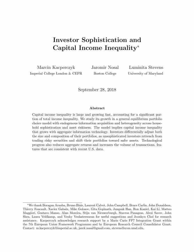
Figure 1 shows the evolution of masses and gains from learning as aggregate capacity grows.

At low capacity, all investors learn about the most volatile asset, but as capacity grows, the

gains from learning about this asset decline, and strategic substitutability in learning pushes

some investors to learn about less volatile assets. The threshold that endogenizes single-asset

learning as an optimal outcome is given by �1 ⌘q

1+⇢

2⇠1

1+⇢

2⇠2

� 1. For capacity above �1, at

least two assets are learned about and for su�ciently high information capacity, all assets

are learned about.12 Nevertheless, not all assets are learned about with the same intensity:

The mass of investors who learn about an asset is decreasing in its volatility. This allocation

12thus endogenizing the assumption employed in models with exogenous signals.

13

of attention a↵ects the holdings across assets, and hence the investors’ portfolio returns.

Proposition 4 (Symmetric Growth). Let k 1 be the number of assets actively traded in

equilibrium. Consider an increase in aggregate capacity � generated by a symmetric growth

in capacities to K

01 = (1 + �)K1 and K

02 = (1 + �)K2, � 2 (0, 1). Let k0 � k denote the new

number of actively traded assets. For i 2 {1, ..., k0},

(i) Average asset prices increase and average excess returns decrease, approaching the risk

free rate in the limit.

(ii) Average ownership share of sophisticated investors E [q1i] /x increases and average own-

ership share of unsophisticated investors E [q2i] /x decreases, and the gap is increasing in

asset volatility.

(iii) As long as the return on the risky portfolio exceeds the risk-free rate, average capital

income gets more unequal, as E [⇡1i] /E [⇡2i] increases, with inequality being higher for the

more volatile assets.

Higher capacity to process information means that investors have more precise news

about the realized payo↵s, resulting in lower gains from learning, lower average returns, and

larger and more volatile positions. However, as asset prices increase and returns decline,

inequality keeps increasing. Sophisticated investors increase their ownership share at the

expense of the less sophisticated investors, who retreat. This pecuniary externality arises

regardless of the learning technology, since it is due to the fact that posterior variance

is lower for the sophisticated investors, and hence on average they want to hold a larger

quantity than the unsophisticated investors. Moreover, the increase in ownership is larger

for the more volatile assets that have higher gains from learning and generate higher expected

14

returns. Hence, asset heterogeneity combined with endogenous information choice generates

di↵erential ownership growth that in turn amplifies the growth in inequality.

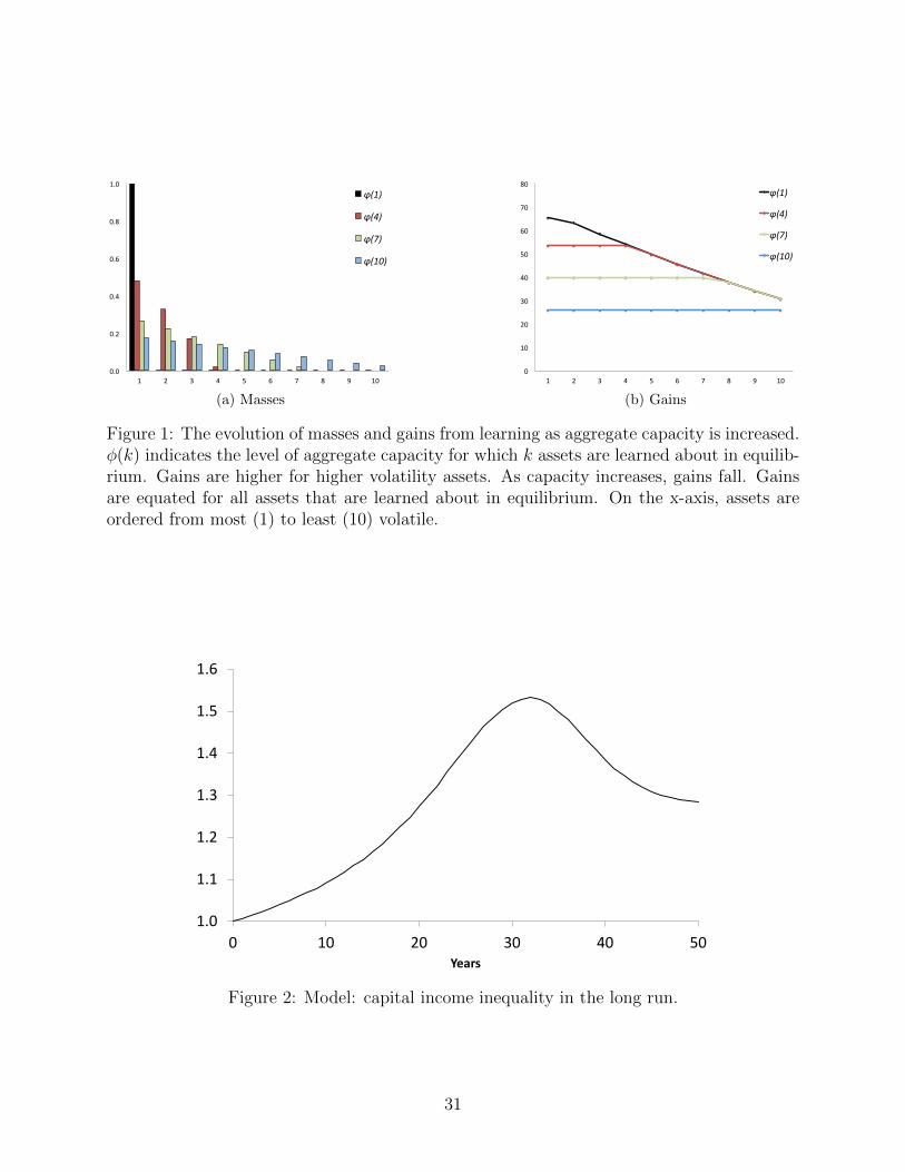
As capacity continues to grow, the decline in returns eventually becomes a mitigating

factor in the growth of income inequality. Intuitively, if market returns are close to the risk

free rate, then there is less scope in the economy for extracting informational rents. Capital

income inequality peaks as rates of return reach the risk free rate. It subsequently starts to

decline, and eventually, it stabilizes at a level implied by the di↵erences in risk-free return

income earned on on previously accumulated wealth. In the limit, all information is revealed

and capital income inequality becomes flat. This process is shown in Figure 2.

4 Quantitative Analysis

So far, we have found that progress in information technology can qualitatively generate

growing capital income inequality, through changes in both portfolio size and composition

across investors. We now parameterize the model to provide some guidance for the magni-

tudes implied by this mechanism. We use data on household capital income from the SCF

and data on the financial market from CRSP. We parameterize the model based on data

from the first half of the SCF sample (1989-2000), and then we consider an experiment in

which aggregate information capacity in the economy grows at a constant rate, to generate

predictions for the second half of the sample (2001-2013).

15

4.1 Technological Progress and Inequality Growth

Table 1 presents parameter values and targets for the baseline results. The parameters

characterizing the financial market are the risk free rate, r = 2.5%, which matches the 3-

month T-bill rate net of inflation over the period, the number of risky assets, n, which we set

to 10 arbitrarily, and the means and volatilities of payo↵s and noise shocks. In the absence

of detailed information regarding holdings of di↵erent types of securities at the household

level, we target volatility moments from the U.S. equities market. We set the dispersion in

the volatilities of asset payo↵s �i

to target a dispersion in idiosyncratic return volatilities of

3.54, as measured by the the ratio of the 90th percentile to the median of the cross-sectional

idiosyncratic volatility of stock returns.13 We set the volatility of shocks from noise traders to

�

x

= 0.4 to target an average monthly turnover (defined as the total monthly volume divided

by the number of shares outstanding), equal to 9.7%. We normalize the level of prices by

normalizing the mean payo↵ and the mean supply for each asset to z

i

= 10, xi

= 5.14

The investor-level parameters we need to pin down are the risk aversion coe�cient ⇢, the

information capacities of the two investor types (K1, K2), and the fraction of sophisticated

investors (�). We select those parameters to target the market return of 11.9% (correspond-

ing to 1989-2000 average); the fraction of assets that investors learn about, which, in the

absence of empirical guidance, we set to 50%; the equity ownership share of sophisticated

investors of 69%; and the return spread between sophisticated and unsophisticated house-

holds of four percentage points. To compute the last two moments, we use data from the

13We normalize the lowest volatility to �

n

= 1, and we set �

i

= �

n

+ ↵(n � i)/n, which implies thevolatility distribution is linear. The dispersion target generates a slope coe�cient ↵ = 0.65.

14Changing the number of assets in the parameterization does not have a major impact on our results.

16

Survey of Consumer Finances. Although not as comprehensive as tax records data, the

SCF provides detailed information about the balance sheets of a representative sample of

U.S. households.15 We restrict our sample to participants in financial markets, defined as

households that report holding stocks, bonds, mutual funds, receiving dividends, or having

a brokerage account. On average, 34% of households participate.16 We classify as sophisti-

cated investors the participants in the top decile of the wealth distribution, and relatively

unsophisticated investors as the remaining 90% of participants.17 Using this definition, the

equity ownership share of sophisticated investors is 69%.18

In order to quantify the return heterogeneity, for each household, we compute capital

income divided by holdings of risky securities (stocks, bonds, and mutual funds), and then

use these return measures to capture the heterogeneity between the two groups of households.

Specifically, we compute the ratio of the median return of the unsophisticated households

relative to the median return of the sophisticated households, which is 69.2% over the first

half of the sample. We use this gap to obtain targets for the levels of returns of each

household type, given the market return. The weights used in computing the aggregate

return are the fraction of risky securities held by each type of household in the SCF (31%

15We use the weights provided in the public use data sets of the SCF in order to make the resultsrepresentative of the population of U.S. households. These weights account for both the oversampling ofwealthy households and for di↵erential patterns of nonresponse. For a discussion of weights and aggregateanalysis of the quality of SCF data, see Kennickell & Woodburn (1999) and Kennickell (2000). See also Saez& Zucman (2016) for a detailed comparison of the SCF to U.S. administrative tax data. In short, they findthat the SCF is representative of trends and levels of inequality in the U.S., but understates inequality insidethe top 1% of the wealth distribution.

16We also consider a broader measure of participation that includes all households with equity in aretirement account. This raises the participation rates, but does not alter our main findings.

17In the Appendix, we show that in the data people with higher initial wealth use more sophisticatedinvestment instruments, hold larger portfolios, and invest a lower proportion of their assets in money-likeinstruments. Additional evidence that links wealth to investment sophistication includes Calvet et al. (2009)and Vissing-Jorgensen (2004).

18To compute the number, we first compute the dollar value of the risky part of the financial holdingsof households (stocks, bonds, non-money market funds, and other financials) for each decile of the wealthdistribution. Then, we compute the share of these risky assets held by the top decile.

17

versus 69%). That gives us the di↵erence between sophisticated and unsophisticated returns

of four percentage points, which together with the target for market return above implies

the target for sophisticated return of 13.1% and the unsophisticated return of 9.1%.19

Table 2 presents the model’s response to aggregate capacity growth chosen to match

the market return in the entire sample of 7%. It implies a 4.9% growth in capacity and

additionally generates an increase in trading volume, as better informed investors adjust their

holdings more aggressively. Quantitatively, a capacity growth of 4.9% over 24 years generates

a decline in market returns to 2.6%, bringing the average return for the entire period to 7%,

as in the data, while turnover increases from 9.7% in the first half of the sample to 16.8% in

the second half, versus 16.0% in the data. This technological progress leads to higher capital

income inequality, which grows by 38% over the period. This figure suggests that aggregate

capacity growth is quite potent in generating capital income inequality growth. For reference,

in the corresponding period capital income inequality growth in the SCF equals 87%.20

Inequality grows due to two main e↵ects: (i) larger relative exposure of sophisticated

investors to the asset market, marked by higher ownership shares across all assets, and (ii)

a shift of sophisticated investors towards high risk, high return assets and that of unso-

phisticated investors towards lower risk and lower return assets. As capacity increases, less

sophisticated investors are priced out of trading the more risky assets and shift their portfolio

weights towards less risky, lower-return assets. As a result, the ownership share of sophis-

ticated investors, relative to their population share, rises relatively more for the assets that

19We perform a detailed grid search over parameters until all the simulated moments are within a 10%distance from target. That gives sophisticated ownership within 0.7%, sophisticated and unsophisticatedreturns within 7%, ratio of volatilities within 2% and all other targets matched exactly.

20We compute this inequality growth as follows. For each survey year, we sort the sample of participantsby the level of total wealth, and we calculate inequality as the ratio of average capital income of the top 10%to that of the bottom 90% of participants.

18

are above the median in terms of volatility relative to the assets that are below the median

in terms of volatility. For both types of assets, sophisticated owners are over-represented

relative to their size in the population (both numbers are greater than 1), reflecting their

larger overall portfolios. But the di↵erence is larger for the more volatile assets: at the end

of the simulation period, sophisticated investors hold 21% more of high-risk assets relative

to their population weight, compared to 14% more for low-risk assets. This gap measures

the retrenchment of unsophisticated investors from the most profitable assets.

To isolate the e↵ects due to portfolio composition and volatility dispersion, we solve and

parameterize our model with just one risky asset. In a one asset economy, the rates of return

on risky portfolios–which we use in the calibration of the benchmark model–are the same

across the two types of investors, since there is now only one risky asset. The di↵erences

in capital income come only from the di↵erences in holdings of the risky asset, both on

average and state by state. Hence, we use ownership and turnover to discipline the one-asset

numerical exercise. The resulting growth in capital income inequality is almost half of the

growth generated by the benchmark model: 20% versus 38%. Hence, the di↵erent exposure

to assets with di↵erent characteristics, and the asymmetric shifting of weights across assets

as capacity grows play a significant role in driving capital income inequality.21

Our growth simulation increases the relative share of the sophisticated group in the

21In terms of the parameterization, the model with one risky asset takes away three targets from thebenchmark model: heterogeneity in asset volatility, fraction of actively traded assets, and the return di↵erencebetween sophisticated and unsophisticated investors. We keep the value of the risk aversion coe�cient thesame as in the benchmark model and set the volatility of the single asset payo↵ equal to the median payo↵volatility of the benchmark model. That leaves three parameters: volatility of the noise trader demand�

x

, and the two capacities of sophisticated and unsophisticated investors. We choose these to match: theaverage market return, the average asset turnover, and the share of sophisticated ownership. That gives(K1,K2,�x

) = (0.0544, 0.0163, 0.37). In the dynamic simulation, we pick the growth rate of aggregatecapacity to match the decline in the market return (just as in the benchmark simulation). That implies a6.7% growth rate of technology.

19

economy’s total information capacity �. To quantify the relevance of this force, we consider

a simulation in which we grow capacity di↵erentially so as to keep the shares of relative

capacity of the investor types constant at the levels in the initial period. This change results

in an inequality growth of 32% versus the benchmark 38%. The relatively limited e↵ect

reflects the fact that the sophisticated share in overall capacity is high to begin with.22

Calibrating the information capacity growth is challenging because the information that

investors have when they make their investment decisions is not observable. Hence, our

strategy is to set capacity growth so as to match the decline in market returns seen in the

data, and to complement these results with robustness checks on this growth rate. We

consider two alternative annual growth rates: 4% and 8%, based on the annual growth rate

of the number of stocks actively analyzed by the financial industry, and the growth rate of

the number of analysts per stock in the financial industry, respectively.23 These rates imply

24% and 60% inequality growth. Although the results are sensitive to the growth rate of

information capacity, the model generates a quantitatively significant rise in capital income

inequality relative to the data.

4.2 Robustness

Two features of our specification have important implications for our results: the infor-

mation acquisition technology and the equilibrium selection mechanism. We now discuss

how changing our assumptions along these two dimensions a↵ects inequality.

22In the Online Appendix, we also provide an exercise in which the capacity grows in proportion tothe rates of return of the portfolio, capturing explicitly the idea that capacity is linked to wealth. Thatexacerbates the growth in inequality. Keeping the average capacity growth the same as in the benchmarkeconomy, linking capacity growth to returns implies a 49% increase in capital income inequality.

23Our information friction implies that growth in information capacity translates into growth in activelyanalyzed stocks, and also more information capacity allocated per stock, consistent with these growth trends

20

Marginal Cost Predictions In our benchmark model, we endow each investor with some

level of capacity to process information. What happens to investor choices and inequal-

ity if we model a marginal cost of acquiring information instead? Let investors di↵er in

their marginal cost of information, 0 < 1 < 2. Then the investor’s objective becomes

max{vji}ni=1

Pn

i=1

hG

i

�

2i

b�2ji� j

2 log �

2i

b�2ji

i, and the information problem is independent across as-

sets as investors decide how much information to purchase for each asset separately. Hence,

instead of a corner solution for learning, each investor purchases information about all assets

whose gains exceed their marginal cost, up to the point at which the gain from learning

reaches the marginal cost. In equilibrium, the gains from learning decline endogenously the

more information investors purchase and the sophisticated, low marginal cost investors are

the marginal buyers of information, driving the gains from learning down to their marginal

cost for all assets. The unsophisticated investors, who have a higher marginal cost, are

now priced out of the information market altogether. As in the benchmark case, there is

a preference for volatility, with the quantity of information purchased declining with asset

volatility. The di↵erence is that now for each asset, either the gains from learning are too

small relative to the costs that neither investor learns about it, or only the sophisticated

investors learn about it. For a given amount of information in the economy, the marginal

cost specification results in larger inequality in both holdings and capital income relative to

the endowed capacity case, in which both types of investors learn. Moreover, technological

progress in information processing has no direct e↵ect on the unsophisticated investors: As

long as their marginal cost remains above that of the sophisticated investor, they purchase

no information and invest in all assets according to their prior beliefs.

21

Asymmetric Equilibrium Predictions In our benchmark model, we pin down the total

amount of capacity devoted to each asset, but not the contribution of each investor group

to that total. When deriving our analytic and numerical results, we impose a symmetric

equilibrium, assuming that the fraction of investors that learn about each asset is the same

for both investor types. We base this assumption on our result that the gains from learning

about di↵erent assets are the same for both sophisticated and unsophisticated investors.

However, the same equilibrium allocation of attention (and hence asset prices) could be

achieved with a di↵erent distribution of investors across assets. How sensitive are our results

to deviations from the symmetric equilibrium? First, it is useful to note that all our results

hold at the individual level: If we compare two investors who both monitor the same asset,

one sophisticated and one unsophisticated, they will di↵er in their holdings, capital income,

and response to capacity growth as expected. But when we compare the average holdings of

the two groups, asset-level predictions depend on how many investors learn about the asset

in each group. It is possible to conceive of an allocation of investors across assets such that

for some assets, the per capita ownership of unsophisticated investors is larger than that of

the sophisticated investors. But it remains the case that on average across all assets the per

capita ownership–and hence capital income–of the unsophisticated investors is strictly lower

than that of the sophisticated investors. Moreover, growth in aggregate capacity continues to

increase capital income inequality (as long as returns remain above the risk free rate), even

if we consider a reshu✏ing of masses most advantageous to the unsophisticated investors,

namely one that assigns all the unsophisticated investors learning about an asset to the

highest volatility asset. Such a reshu✏ing yields positive, albeit lower, inequality growth.

Numerically, we find that in our parameterized economy such a reshu✏ing has minimal

22

e↵ects on inequality growth (reducing it by less than one percentage point), because the

data favor a parameterization in which the unsophisticated investors contribute minimally

to the allocation of attention for each asset, so that how we reshu✏e them across assets has

very limited e↵ects on the dispersion of ownership and capital income.

5 Empirical Evidence

We now provide auxiliary evidence supporting our mechanism and its implications.

Skill versus Risk How much of the growth in inequality comes from di↵erences in expo-

sure to risk versus di↵erences in skill? Our model is one in which both risk-taking di↵erences

and pure compensation for skill generate return heterogeneity. Sophisticated investors are

more exposed to risk because they choose to hold a larger share of risky assets (compensa-

tion for risk); and because they have an informational advantage (compensation for skill).

Quantitatively, in our model the compensation for skill accounts for approximately 75% of

the return di↵erential between the two investor groups, with the remaining 25% reflecting

more risk taking.24

Empirically, Fagereng et al. (2016a) document that risk taking is only partially responsi-

ble for the di↵erence in returns among Norwegian households, with approximately half of the

return di↵erence being attributed to unobservable heterogeneity. Corroborating this finding,

we consider more aggregated data from the U.S. financial market. We compare returns from

di↵erent types of mutual funds, using data from Morningstar, which contains information

for two types of funds: those with a minimum investment of $100,000 (institutional funds)

24The Appendix presents the details of the calculation.

23

and those without such restrictions (retail funds). These two types of funds are suggestive

of the kind of investment returns sophisticated versus unsophisticated investors can access.

Since the institutional funds have a minimum investment threshold, less sophisticated, less

wealthy investors do not have access to the higher returns earned by institutional funds,

even for “plain vanilla” assets like equities.25 Our fund data span the period 1989 through

2012. We compare the returns of the two groups adjusting for di↵erences in exposure to

common risk factors, a methodology that is standard in asset pricing literature. Our choice

of common risk factors follows Carhart (1997) and includes market excess returns, return

on the size factor, return on the value factor, and return on the momentum factor. To com-

pute quantitative di↵erences between the two investor groups we calculate a hedge portfolio,

defined as a di↵erence between monthly returns on the sophisticated portfolio and monthly

returns on the unsophisticated portfolio. We then estimate the time-series regression of the

hedge returns on the four factors. Our coe�cient of interest is an intercept, which measures

abnormal returns over and above premia for risk. The hedge portfolio generates a statis-

tically significant positive return of 33 basis points per month, which is almost 4% on an

annual basis. Hence, we conclude that di↵erences in risk exposures alone are unlikely to

explain the di↵erences in returns between sophisticated and unsophisticated investors.

Nevertheless, by shutting down the risk aversion channel, we are likely minimizing the

e↵ect that risk has on inequality outcomes. The overall growth in inequality can be increased

by assuming either decreasing absolute risk aversion or di↵erences in risk attitudes that, like

information capacity, are correlated with wealth. The less risk averse investors would hold

25In the Appendix, we present additional evidence that the there are both institutional and informa-tional barriers that prevent unsophisticated households from gaining access and delegating their investmentdecisions to high quality investment services.

24

a greater share of risky assets, and hence they would have higher expected capital income.26

In a CRRA framework, the model solution under no capacity di↵erences predicts the same

portfolio shares for risky assets, independent of wealth. Intuitively, if agents have common

information, then wealth di↵erences a↵ect the composition of their allocations between the

risk-free asset and the risky portfolio, but not the composition of the risky portfolio, which

is determined optimally by the (common) belief structure. As a result, di↵erences in ca-

pacity are a necessary component for the model to generate any risky return di↵erences

across agents. Similarly, within our mean-variance specification, a growing di↵erence in risk

aversion produces growing aggregate ownership in risky assets of less risk averse investors,

and a uniform, proportional retrenchment from all risky assets of more risk averse investors.

However, heterogeneity in risk aversion alone cannot generate the empirical investor-specific

rates of return on equity, di↵erences in portfolio weights within a class of risky assets or dif-

ferential growth in ownership by asset volatility. Hence, the information asymmetry remains

central to matching several recent trends in U.S. financial markets.27

The Extensive Margin of Limited Participation Limited participation in U.S. finan-

cial markets has long been a source of inequality in total income and wealth (e.g., Mankiw

& Zeldes (1991)). How important is the limited participation margin for generating capi-

tal income inequality? Using data from the SCF, we find that much of the recent growth

in financial wealth inequality has occurred among household who participate in financial

markets, and that trends in capital income growth mirror trends in total financial wealth

26Such setting would also encompass situations in which investors are exposed to di↵erent levels of volatil-ity in areas outside capital markets, like labor income.

27Additionally, Gomez (2016) shows that when macro asset pricing models with heterogenous risk aversionare parameterized to match the volatility of asset prices, they require a degree of heterogeneity in preferencesthat leads to counterfactual predictions about wealth inequality.

25

inequality. Our evidence on capital income inequality reinforces existing results using more

detailed U.S. and European data, e.g. Saez & Zucman (2016), Fagereng et al. (2016b) and

Bach et al. (2015).

First, participation is hump-shaped over time. Moreover, inequality in total financial

wealth has grown within the group of households who participate in financial markets, but

it has remained essentially unchanged along the extensive margin (defined as the ratio of

average financial wealth of the bottom 10% of participating households to that of the non-

participating households). Thus the dynamics of financial wealth inequality do not appear

to be driven by the participation margin. These trends are shown in Figure 3 and Figure 4.28

Second, among participants, the increase in inequality in financial wealth tracks the

accumulation of capital income from the risky assets (namely, income from dividends, interest

income, and realized capital gains). To see this, we consider the counterfactual financial

wealth obtained from accruing capital income only.29 Figure 5 suggests that past capital

income realizations may be su�cient to explain the evolution of financial wealth inequality,

without resorting to mechanisms that involve savings rates from other income sources.30

Third, among participating households, capital income inequality is large and growing

fast. Panel (a) of Figure 7 shows that in the cross-section, capital income is an order of

magnitude more unequal than either labor or total income. For example, in 1989, the

average capital income of the top 10% of participants was 21 times larger than that of the

28Financial wealth in the SCF contains holdings of risky assets (stocks, bonds, mutual funds), passiveassets (life insurance, retirement accounts, royalties, annuities, trusts), and liquid assets (cash, checking andsavings accounts, money market accounts).

29For example, the counterfactual financial wealth level in 1995 is equal to the actual financial wealth in1989 plus 3 times the capital income reported in the prior survey years (in this case, 1989 and 1992).

30By construction, the two wealth levels are identical in 1989, so the figure also implies that the coun-terfactual levels of financial wealth for each group are very close to those in the data. Still, we treat thisevidence as suggestive, since our exercise imposes a panel interpretation on a repeated cross-section.

26

bottom 90% of participants. This ratio increased to nearly 40 in 2013. By comparison,

the corresponding ratio for wage income was 2.4 in 1989 and 3.9 in 2013. To compare the

dynamics of inequality across income sources, we normalize the inequality of each income

measure to 1 in 1989, and plot growth rates for capital, labor, and total income inequality

in panel (b) of the figure. As is well known, labor income inequality has grown significantly

during this period, and so has capital income inequality, which nearly doubled.

We complement this evidence with additional data on flows into and out of mutual funds

from Morningstar by sophisticated (institutional) and unsophisticated (retail) investors. As

shown in Figure 6, the cumulative flows from sophisticated investors into equity and non-

equity funds increase steadily over the entire sample period. In contrast, since 2000, unso-

phisticated investors have been shifting their funds out of equity mutual funds and into less

risky non-equity funds. To the extent that direct equity holdings are more risky than diversi-

fied equity portfolios, such as mutual funds, this implies that unsophisticated investors have

been systematically reallocating their wealth from riskier to safer asset classes. This trend

is consistent with our model, which predicts that as aggregate capacity grows, sophisticated

investors expand their ownership of risky assets by order of volatility: starting from the

highest volatility assets and then moving down.

6 Concluding Remarks

What contributes to the growing capital income inequality across households? We pro-

pose a theoretical information-based framework that links capital income to investor sophis-

tication. Our model implies income inequality that rises with the total information in the

27

market. Predictions on asset ownership, market returns, and turnover provide additional

support for the economic mechanism we propose.

The overall growth of investment resources and competition among investors with dif-

ferent skill levels are generally considered signs of a well-functioning financial market. Our

work highlights how advances in information processing technologies also have consequences

beyond the financial market, a↵ecting the distribution of income.

References

Admati, Anat (1985), “A noisy rational expectations equilibrium for multi-asset securities markets,”Econometrica 53(3): 629–657.

Aiyagari, Rao S. (1994), “Uninsured idiosyncratic risk and aggregate saving,” Quarterly Journal

of Economics 109(3): 659–684.

Arrow, Kenneth J (1987), “The demand for information and the distribution of income,” Probability

in the Engineering and Informational Sciences 1(01): 3–13.

Atkinson, Anthony B, Thomas Piketty & Emmanuel Saez (2011), “Top incomes over a century ormore,” Journal of Economic Literature 49: 3–71.

Bach, Laurent, Laurent Calvet & Paolo Sodini (2015), “Rich pickings? Risk, return, and skill inthe portfolios of the wealthy,” Working Paper Stockholm School of Economics.

Benhabib, Jess & Alberto Bisin (2017), “Skewed wealth distributions: Theory and empirics,”Journal of Economic Literature forthcoming.

Benhabib, Jess, Alberto Bisin & Shenghao Zhu (2011), “The distribution of wealth and fiscal policyin economies with finitely lived agents,” Econometrica 79(1): 123–157.

Cagetti, Marco &Mariacristina De Nardi (2006), “Entrepreneurship, frictions, and wealth,” Journalof Political Economy 114: 835–870.

Calvet, Laurent E, John Y Campbell & Paolo Sodini (2009), “Measuring the financial sophisticationof households,” American Economic Review 99(2): 393–398.

Cao, Dan & Wenlan Luo (2017), “Persistent heterogeneous returns and top end wealth inequality,”Review of Economic Dynamics 26: 301–326.

Carhart, Mark M. (1997), “On persistence in mutual fund performance,” Journal of Finance 52:57–82.

28

Chien, YiLi, Harold Cole & Hanno Lustig (2011), “A multiplier approach to understanding themacro implications of household finance,” Review of Economic Studies 78 (1): 199–234.

De Nardi, Mariacristina & Giulio Fella (2017), “Saving and wealth inequality,” CEPR WorkingPaper 11746.

Fagereng, Andreas, Luigi Guiso, Davide Malacrino & Luigi Pistaferri (2016a), “Heterogeneity andpersistence in returns to wealth,” NBER Working Paper No 22822.

Fagereng, Andreas, Luigi Guiso, Davide Malacrino & Luigi Pistaferri (2016b), “Heterogeneity inreturns to wealth and the measurement of wealth inequality,” The American Economic Review

106(5): 651–655.

Favilukis, Jack (2013), “Inequality, stock market participation, and the equity premium,” Journal

of Financial Economics 107 (3): 740–759.

Gabaix, Xavier, Jean-Michel Lasry, Pierre-Louis Lions & Benjamin Moll (2016), “The dynamics ofinequality,” Econometrica 84(6): 2071–2111.

Gomez, Matthieu (2016), “Asset prices and wealth inequality,” Working Paper Princeton Univer-sity.

Greenwood, Daphne (1983), “An estimation of US family wealth and its distribution from micro-data,” Review of Income and Wealth 29 (1): 23–44.

Guvenen, Fatih (2007), “Do stockholders share risk more e↵ectively than non-stockholders?” Re-

view of Economics and Statistics 89(2): 275–288.

Guvenen, Fatih (2009), “A parsimonious macroeconomic model for asset pricing,” Econometrica

77(6): 1711–1750.

Kasa, Kenneth & Xiaowen Lei (2018), “Risk, uncertainty, and the dynamics of inequality,” Journal

of Monetary Economics 94: 60–78.

Kennickell, Arthur B (2000), “Wealth measurement in the Survey of Consumer Finances: Method-ology and directions for future research,” .

Kennickell, Arthur B & R Louise Woodburn (1999), “Consistent Weight Design for the 1989, 1992and 1995 SCFs, and the Distribution of Wealth,” Review of Income and Wealth 45(2): 193–215.

Kessler, Dennis & Edward N. Wol↵ (1991), “A comparative analysis of household wealth patternsin France and the United States,” Review of Income and Wealth 37 (1): 249–266.

Krusell, Per & Anthony A. Smith (1998), “Income and wealth heterogeneity in the macroeconomy,”Journal of Political Economy 106(5): 867–896.

Lusardi, Annamaria, Pierre-Carl Michaud & Olivia S. Mitchell (2017), “Optimal financial knowl-edge and wealth inequality,” Journal of Political Economy forthcoming.

Mackowiak, Bartosz &MirkoWiederholt (2009), “Optimal sticky prices under rational inattention,”American Economic Review 99 (3): 769–803.

29

Mackowiak, Bartosz & Mirko Wiederholt (2015), “Business cycle dynamics under rational inatten-tion,” The Review of Economic Studies 82(4): 1502–1532.

Mankiw, N Gregory & Stephen P Zeldes (1991), “The consumption of stockholders and nonstock-holders,” Journal of Financial Economics 29(1): 97–112.

Matejka, Filip (2015), “Rationally inattentive seller: Sales and discrete pricing,” The Review of

Economic Studies 83(3): 1125–1155.

Mondria, Jordi (2010), “Portfolio choice, attention allocation, and price comovement,” Journal of

Economic Theory 145(5): 1837–1864.

Pastor, Lubos & Pietro Veronesi (2016), “Income inequality and asset prices under redistributivetaxation,” Journal of Monetary Economics 81: 1–20.

Peng, Lin (2005), “Learning with information capacity constraints,” Journal of Financial and

Quantitative Analysis 40(2): 307–329.

Peng, Lin & Wei Xiong (2006), “Investor attention, overconfidence and category learning,” Journal

of Financial Economics 80(3): 563–602.

Peress, Joel (2004), “Wealth, information acquisition and portfolio choice,” The Review of Financial

Studies 17(3): 879–914.

Piketty, Thomas (2014), Capital in the Twenty-First Century, Harvard University Press.

Piketty, Thomas & Emmanuel Saez (2003), “Income inequality in the United States, 1913–1998,”The Quarterly Journal of Economics 118(1): 1–41.

Quadrini, Vincenzo (1999), “The importance of entrepreneurship for wealth concentration andmobility,” Review of Income and Wealth 45(1): 1–19.

Saez, Emmanuel & Gabriel Zucman (2016), “Wealth inequality in the United States since 1913:Evidence from capitalized income tax data,” The Quarterly Journal of Economics 131(2): 519–578.

Shannon, Claude E (1948), “A mathematical theory of communication,” Bell System Technical

Journal 27: 379–423 and 623–656.

Sims, Christopher A (2003), “Implications of rational inattention,” Journal of Monetary Economics

50(3): 665–690.

Stevens, Luminita (2018), “Coarse pricing policies,” Working Paper, University of Maryland.

Van Nieuwerburgh, Stijn & Laura Veldkamp (2009), “Information immobility and the home biaspuzzle,” Journal of Finance 64(3): 1187–1215.

Van Nieuwerburgh, Stijn & Laura Veldkamp (2010), “Information acquisition and under-diversification,” Review of Economic Studies 77(2): 779–805.

Vissing-Jorgensen, Annette (2004), “Perspectives on behavioral finance: Does “irrationality” disap-pear with wealth? Evidence from expectations and actions,” in NBER Macroeconomics Annual

2003, Vol. 18, pp. 139–208, The MIT Press, Cambridge.

30

0.0

0.2

0.4

0.6

0.8

1.0

1 2 3 4 5 6 7 8 9 10

φ(1)

φ(4)

φ(7)

φ(10)

(a) Masses

0

10

20

30

40

50

60

70

80

1 2 3 4 5 6 7 8 9 10

φ(1)

φ(4)

φ(7)

φ(10)

(b) Gains

Figure 1: The evolution of masses and gains from learning as aggregate capacity is increased.�(k) indicates the level of aggregate capacity for which k assets are learned about in equilib-rium. Gains are higher for higher volatility assets. As capacity increases, gains fall. Gainsare equated for all assets that are learned about in equilibrium. On the x-axis, assets areordered from most (1) to least (10) volatile.

1.0

1.1

1.2

1.3

1.4

1.5

1.6

0 10 20 30 40 50Years

Figure 2: Model: capital income inequality in the long run.

31

0.0

0.1

0.2

0.3

0.4

0.5

0.6

1989 1992 1995 1998 2001 2004 2007 2010 2013

Par0cipa0on

Par0cipa0on+Re0rement

Figure 3: Financial markets participation in the SCF. Participants are individuals who havea brokerage account or who report stock holdings, bonds, money market funds, or non-money market funds. For a broader measure, we also consider households who have equityin retirement accounts.

32

0.5

0.8

1.0

1.3

1.5

1.8

2.0

1989 1992 1995 1998 2001 2004 2007 2010 2013

Bo.om90/Non-par7cipants

Top10/Bo.om90

Bo.om10/Non-par7cipants

Figure 4: Extensive and intensive margins in financial wealth inequality in the SCF. ’Top10/Bottom 90’ measures inequality within the group of participants, defined as the ratioof financial wealth of the top wealth decile to that of the bottom 90% of participants.’Bottom 10/Non-participants’ measures inequality at the participation margin, measured asthe ratio of financial wealth of the bottom 10% of participating households to that of allnon-participating households.

33

0

5

10

15

20

25

1989 1992 1995 1998 2001 2004 2007 2010 2013

Top10/Bo0om90Actual

Top10/Bo0om90Counterfactual

Figure 5: Financial wealth inequality and counterfactual financial wealth inequality con-structed by accruing capital income.

34

0

2E+11

4E+11

6E+11

8E+11

1E+12

1.2E+12

1.4E+12

1.6E+12

198901

198911

199009

199107

199205

199303

199401

199411

199509

199607

199705

199803

199901

199911

200009

200107

200205

200303

200401

200411

200509

200607

200705

200803

200901

200911

201009

201107

201205

Non-EquityMutualFunds

EquityMutualFunds

(a) Institutional

0

2E+11

4E+11

6E+11

8E+11

1E+12

1.2E+12

1.4E+12

1.6E+12

1.8E+12

2E+12

198901

198911

199009

199107

199205

199303

199401

199411

199509

199607

199705

199803

199901

199911

200009

200107

200205

200303

200401

200411

200509

200607

200705

200803

200901

200911

201009

201107

201205

Non-EquityMutualFunds

EquityMutualFunds

(b) Retail

Figure 6: Cumulative Flows to Mutual Funds: Institutional versus Retail Funds. Morn-ingstar data.

0

10

20

30

40

50

60

70

1989 1992 1995 1998 2001 2004 2007 2010 2013

CapitalIncomeInequalityTotalIncomeInequalityLaborIncomeInequality

(a) Raw

0.0

0.5

1.0

1.5

2.0

2.5

3.0

3.5

1989 1992 1995 1998 2001 2004 2007 2010 2013

CapitalIncomeInequalityTotalIncomeInequalityLaborIncomeInequality

(b) Normalized

Figure 7: Income inequality growth in the SCF. Inequality is the ratio of the top 10% to thebottom 90% (in terms of total wealth) of participants in financial markets. (a) Inequalityfor capital income, labor income and other income in levels. (b) Same series, normalized to1 in 1989.

35

Table 1: Parameter Values in the Baseline Model

Parameter Symbol Value Target (1989-2000 averages)

Risk-free rate r 2.5% 3-month T-bill � inflation = 2.5%

Number of assets n 10 Normalization

Vol. of asset payo↵s �

i

2 [1, 1.59] p90/p50 of idio. return vol = 3.54

Vol. of noise shocks �

xi

0.4 for all i Average turnover = 9.7%

Mean payo↵, supply z

i

, xi

10, 5 for all i Normalization

Risk aversion ⇢ 1.032 Average return = 11.9%

Information capacities K1, K2 0.37, 0.0037, Sophisticated share = 69%

and investor masses � 0.675 Share actively traded = 50%

Sophisticated return = 13.1%

Note: Data are from CRSP for idiosyncratic stock return volatility, turnover, and averagereturn and from SCF for return spread and sophisticated ownership share. Targets are for the1989-2000 period.

36

Table 2: Aggregate Capacity Growth Outcomes

Statistic Baseline DataCapacity growth (%) 4.9

Average market return (%) 7 7

Capital income inequality growth (%) 38 87

Sophis ending ownership share, top 1.21

Sophis ending ownership share, bottom 1.14

One asset Low growth High growthCapacity growth (%) 6.7 4 8

Average market return (%) 7 8 5

Capital income inequality growth (%) 20 24 60

Sophis ending ownership share, top 1.1 1.16 1.43

Sophis ending ownership share, bottom 1.08 1.41

Note: The average market return is the market return over the entire 1989-2013 period, and istargeted in the baseline and one-asset economy. All other numbers are not targeted. “Sophis own-ership share” represents the ownership share of sophisticated investors, relative to their populationshare, for the assets that are above the median in terms of volatility (“top”) and for assets thatare below the median in terms of volatility (“bottom”), at the end of the simulation period. In theone-asset economy, it represents the sophisticated ownership share in the one risky asset.

37

Investor Sophistication andCapital Income InequalityONLINE APPENDIX

Marcin KacperczykImperial College

Jaromir NosalBoston College

Luminita StevensUniversity of Maryland

Abstract

This file contains supplementary material for the paper ‘Investor Sophistication andCapital Income Inequality’, by Kacperczyk, Nosal, and Stevens.

Contents

1 Appendix: Proofs 11.1 Model . . . . . . . . . . . . . . . . . . . . . . . . . . . . . . . . . . . . . . . 11.2 Analytic Results . . . . . . . . . . . . . . . . . . . . . . . . . . . . . . . . . 61.3 Additional Results . . . . . . . . . . . . . . . . . . . . . . . . . . . . . . . . 7

1.3.1 Asymmetric Capacity Growth . . . . . . . . . . . . . . . . . . . . . . 71.3.2 Endogenous Capacity Choice . . . . . . . . . . . . . . . . . . . . . . 71.3.3 CRRA Utility Specification . . . . . . . . . . . . . . . . . . . . . . . 91.3.4 Expansion of Asset Space . . . . . . . . . . . . . . . . . . . . . . . . 121.3.5 Skill versus Risk . . . . . . . . . . . . . . . . . . . . . . . . . . . . . 12

2 Appendix: Additional Data Discussion and Analysis 132.1 Data Constructs . . . . . . . . . . . . . . . . . . . . . . . . . . . . . . . . . . 142.2 Participation . . . . . . . . . . . . . . . . . . . . . . . . . . . . . . . . . . . 152.3 Capital Income . . . . . . . . . . . . . . . . . . . . . . . . . . . . . . . . . . 182.4 Survey of Consumer Finances: Descriptive Statistics . . . . . . . . . . . . . . 192.5 Mutual Funds and Delegation . . . . . . . . . . . . . . . . . . . . . . . . . . 212.6 Expansion of Ownership . . . . . . . . . . . . . . . . . . . . . . . . . . . . . 23

List of Figures

1 Inequality in information capacity (K1

/K2

) as a function of a and absoluterisk aversion coe�cient of the wealthy. . . . . . . . . . . . . . . . . . . . . . 9

2 Financial markets participation in the SCF. . . . . . . . . . . . . . . . . . . 163 Extensive and intensive margins in capital income inequality. . . . . . . . . . 174 Capital income inequality. . . . . . . . . . . . . . . . . . . . . . . . . . . . . 185 Capital income inequality for di↵erent measures of participation. . . . . . . . 196 Cumulative market return on a 15-year passive investment in the U.S. stock

market. . . . . . . . . . . . . . . . . . . . . . . . . . . . . . . . . . . . . . . 217 Cumulative investment returns in equity mutual funds by investor type. . . . 228 Distribution of equity funds’ returns. . . . . . . . . . . . . . . . . . . . . . . 229 Cumulative Flows to Mutual Funds: Institutional vs. Retail . . . . . . . . . 24

2

1 Appendix: Proofs

1.1 Model

Portfolio Choice. In the second stage, each investor chooses portfolio holdings qji

to solve

max{qji

}ni=1

Uj

= Ej

(Wj

)� ⇢

2

Vj

(Wj

) s.t. Wj

= r (W0j

�P

n

i=1

qji

pi

) +P

n

i=1

qji

zi

,

where Ej

and Vj

denote the mean and variance conditional on investor j’s information set:

Ej

(Wj

) = Ej

[rW0j

+P

n

i=1

qji

(zi

� rpi

)] = rW0j

+P

n

i=1

qji

[Ej

(zi

)� rpi

] ,

Vj

(Wj

) = Vj

[rW0j

+P

n

i=1

qji

(zi

� rpi

)] =P

n

i=1

q2ji

Vj

(zi

) .

Let bµji

⌘ Ej

[zi

] and b�2

ji

⌘ Vj

[zi

]. The investor’s portfolio problem is to maximize

Uj

= rW0j

+P

n

i=1

qji

(bµji

� rpi

)� ⇢

2

Pn

i=1

q2ji

b�2

ji

.

The first order conditions with respect to qji

yield qji

= bµji

�rp

i

⇢b�2ji

. Since W0j

does not a↵ect

the optimization, we normalize it to zero. The indirect utility function becomes

Uj

= 1

2⇢

Pn

i=1

(bµji

�rp

i

)

2

b�2ji

.

Posterior Beliefs. The signal structure, zi

= sji

+ �ji

, implies that

bµji

= z + Cov(s

ji

,z

i

)

�

2sji

(sji

� sji

) = sji

,

b�2

ji

= �2

i

⇣1� Cov

2(s

ji

,z

i

)

�

2sji

�

2i

⌘= �2

�ji

.

Information Constraint. Let H (z) denote the entropy of z, and let H (z|sj

) denote theconditional entropy of z given the vector of signals s

j

. Then

I (z; sj

) ⌘ H (z)�H (z|sj

)(1)

=P

n

i=1

H (zi

)�H (z|sj

)(2)

=P

n

i=1

H (zi

)�P

n

i=1

H (zi

|zi�1, sj

)

(1)

=P

n

i=1

H (zi

)�P

n

i=1

H (zi

|sj

)(3)

=P

n

i=1

H (zi

)�P

n

i=1

H (zi

|sji

) =P

n

i=1

I (zi

; sji

)

where (1) follows from the independence of the payo↵s zi

; (2) follows from the chain rule forentropy, where zi�1 = {z

1

, ..., zi�1

}; (3) follows from the independence of the signals sji

.

For each asset i, the entropy of zi

⇠ N (z, �2

i

) is H (zi

) = 1

2

ln (2⇡e�2

i

) .

The signal structure, zi

= sji

+ �ji

, implies that

1

I (zi

; sji

) = H (zi

) +H (sji

)�H (zi

, sji

) = 1

2

log

✓�

2i

�

2sji

|⌃z

i

s

ji

|

◆= 1

2

log⇣

�

2i

�

2�ji

⌘,

where��⌃

z

i

s

ji

�� = �2

sji

�2

�ji

is the determinant of the variance-covariance matrix of zi

and sji

.

Hence I (zi

; sji

) = 0 if �2

�ji

= �2

i

.

Across assets, I (z; sj

) =P

n

i=1

I (zi

; sji

) = 1

2

Pn

i=1

log⇣

�

2i

�

2�ji

⌘= 1

2

log

✓nQ

i=1

�

2i

�

2�ji

◆ K

j

.

Information Objective. Expected utility is given by

E0j

[Uj

] = 1

2⇢

E0j

hPn

i=1

(bµji

�rp

i

)

2

b�2ji

i= 1

2⇢

Pn

i=1

E0j[(bµji

�rp

i

)

2]b�2ji

= 1

2⇢

Pn

i=1

✓bR

2ji

+

bV

ji

b�2ji

◆,

where bRji

and bVji

denote the ex-ante mean and variance of expected excess returns, bµji

�rpi

.Conjecture (and later verify) that prices are normally distributed, p

i

⇠ N�pi

, �2

pi

�.

bRji

⌘ E0j

(bµji

� rpi

) = z � rpi

,

bVji

⌘ V0j

(bµji

� rpi

) = V ar (bµji

) + r2�2

pi

� 2rCov (bµji

, pi

) .

The signal structure implies that V ar (bµji

) = �2

sji

.

Following Admati (1985), we conjecture (and later verify) that prices are pi

= ai

+bi

"i

�ci

⌫i

,for some coe�cients a

i

, bi

, ci

� 0. We compute Cov (bµji

, pi

) exploiting the fact that posteriorbeliefs and prices are conditionally independent given payo↵s. We obtain

bVji

= �2

sji

+ r2�2

pi

� 2rbi

�2

sji

= (1� rbi

)2 �2

i

+ r2c2i

�2

x

� (1� 2rbi

) b�2

ji

.

Hence the distribution of expected excess returns is normal with mean and variance:

bRji

= z � rai

and bVji

= (1� rbi

)2 �2

i

+ r2c2i

�2

x

� (1� 2rbi

) b�2

ji

.

Expected utility becomes

E0j

[Uj

] = 1

2⇢

Pn

i=1

Gi

�

2i

b�2ji

� 1

2⇢

Pn

i=1

(1� 2rbi

) ,

where Gi

⌘ (1� rbi

)2 + r

2c

2i

�

2x

�

2i

+ (z�ra

i

)

2

�

2i

, and where the second summation is independent of

the investor’s choices.

2

Proof of Lemma 1 (Information Choice). The linear objective function and the con-vex constraint imply that each investor allocates all capacity to learning about a sin-gle asset. Let b�2

ji

= e�2K

ji�2

i

. Then the optimization problem can be written asmax{K

ji

}ni=1

Pn

i=1

Gi

e2Kji s.t.P

n

i=1

Kji

Kj

. Suppose the investor allocates capacity tolearning about 2 assets. WLOG, let these assets be indexed by 1 and 2, and supposeG

2

G1

.Then, K

j1

+Kj2

= Kj

and the value of the objective function is

Pn

i=1

Gi

e2Kji = G1

�e2Kj1 � 1

�+G

2

�e2Kj2 � 1

�+P

n

i=1

Gi

(1)

G1

�e2Kj1 � 1

�+G

1

�e2Kj2 � 1

�+P

n

i=1

Gi

(2)

2G1

�eKj � 1

�+P

n

i=1

Gi

(3)

< G1

�e2Kj � 1

�+P

n

i=1

Gi

,

where (1) follows from the assumption WLOG that G2

G1

, (2) follows from the fact thatfor K

j1

+Kj2

= Kj

, e2Kj1 + e2Kj2 is maximized at Kj1

= Kj2

= Kj

/2, and (3) follows fromthe fact that (e2Kj � 1)2 > 0 for K

j

> 0. This chain of inequalities shows that splittingcapacity across two assets yields strictly lower utility than investing all capacity in a singleasset, even if the gains from learning are equal across assets. Splitting capacity among morethan two assets would lower utility even more.

Let lj

index the asset about which investor j learns. The investor’s objective is�e2Kj � 1

�G

l

j

+P

n

i=1

Gi

. Since e2Kj > 1, the objective is maximized by allocating allcapacity to the asset with the largest utility gain: l

j

2 argmaxi

Gi

. The variance of theinvestor’s posterior beliefs is

b�2

ji

=

(e�2K

j�2

i

if i = lj

,

�2

i

if i 6= lj

.

Conditional Distribution of Signals. Conditional on the realized payo↵, the signal is anormally distributed random variable, with mean and variance given by

E (sji

|zi

) = sji

+ Cov(s

ji

,z

i

)

�

2i

(zi

� z) =

(z +

�1� e�2K

j

�"i

if i = lj

z if i 6= lj

,

V (sji

|zi

) = �2

sji

⇣1� Cov

2(s

ji

,z

i

)

�

2sji

�

2i

⌘=

(�1� e�2K

j

�e�2K

j�2

i

if i = lj

0 if i 6= lj

.

Holdings. Individual portfolio holdings are given by

qji

= bµji

�rp

i

⇢b�2ji

= e

2Kji

(bµji

�rp

i

)

⇢�

2i

.

For the assets that investor j does not learn about, Kji

= 0, and qji

= (z � rpi

) /⇢�2

i

. Thisquantity is the same for all investors, regardless of their type.

3

For the asset that investor j learns about, Kji

= Kj

, and qji

= e2Kj (bµ� rpi

) /⇢�2

i

.

Total holdings for the group of sophisticated investors learning about this asset are

RM1i

qji

dj =RM1i

e

2K1(bµ

ji

�rp

i

)

⇢�

2i

dj = e

2K1

⇢�

2i

⇣RM1ibµji

dj � �m1i

rpi

⌘,

where M1i

is the set of sophisticated investors learning about asset i and m1i

2 [0, 1]denotes the fraction of sophisticated investors learning about asset i. Using the con-ditional distribution of signals,

RM1ibµji

dj = �m1i

⇥z + (1� e�2K1)"

i

⇤, and

RM1i

qji

dj =

�m1i

hz�rp

i

⇢�

2i

+�e2K1 � 1

�z

i

�rp

i

⇢�

2i

i.

Total holdings of this asset by both informed and uninformed sophisticated investors are:

Q1i

=RM1i

qji

dj + �(1�m1i

) (z�rp

i

)

⇢�

2i

= �m1i

hz�rp

i

⇢�

2i

+�e2K1 � 1

�z

i

�rp

i

⇢�

2i

i+ �(1�m

1i

) z�rp

i

⇢�

2i

= �⇣

z�rp

i

⇢�

2i

⌘+ �m

1i

�e2K1 � 1

� ⇣z

i

�rp

i

⇢�

2i

⌘.

Per capita holdings for the sophisticated investors are

q1i

= Q1i

�

=⇣

z�rp

i

⇢�

2i

⌘+m

1i

�e2K1 � 1

� ⇣z

i

�rp

i

⇢�

2i

⌘.

Analogous expressions hold for the unsophisticated investors, with m2i

denoting the fractionof unsophisticated investors learning about asset i :

Q2i

= (1� �)⇣

z�rp

i

⇢�

2i

⌘+ (1� �)m

2i

�e2K2 � 1

� ⇣z

i

�rp

i

⇢�

2i

⌘,

q2i

= Q2i

1��

=⇣

z�rp

i

⇢�

2i

⌘+m

2i

�e2K2 � 1

� ⇣z

i

�rp

i

⇢�

2i

⌘.

Finally, total sophisticated and unsophisticated demand for asset i is

Q1i

+Q2i

=⇣

z�rp

i

⇢�

2i

⌘+ �

i

⇣z

i

�rp

i

⇢�

2i

⌘,

where we define �i

⌘ �m1i

�e2K1 � 1

�+ (1� �)m

2i

�e2K2 � 1

�.

Proof of Lemma 2 (Equilibrium Prices). The market clearing condition for each assetin state (z

i

, xi

) is

RM1i

⇣s

ji

�rp

i

e

�2K1⇢�

2i

⌘dj +

RM2i

⇣s

ji

�rp

i

e

�2K2⇢�

2i

⌘dj + (1�m

1i

�m2i

)⇣

z�rp

i

⇢�

2i

⌘= x

i

,

where M1i

denotes the set of measure m1i

2 [0,�] of sophisticated investors who choose tolearn about asset i, and M

2i

denotes the set of measure m2i

2 [0, 1� �], of unsophisticatedinvestors who choose to learn about asset i.

4

Using the conditional distribution of the signals,RM1i

sji

dj = m1i

⇥z +

�1� e�2K1

�"i

⇤for

the type-1 investors, and analogously for the type-2 investors. Then, the market clearingcondition can be written as ↵

1

z + ↵2

"i

� xi

= ↵1

rpi

, where

↵1

⌘ 1+m1i(e2K1�1)+m2i(e2K2�1)⇢�

2i

and ↵2

⌘ m1i(e2K1�1)+m2i(e2K2�1)⇢�

2i

.

We obtain identification of the coe�cients in pi

= ai

+ bi

"i

� ci

⌫i

as

ai

= 1

r

hz � x

↵1

i, b

i

= ↵2r↵1

, and ci

= 1

r↵1.

Let �i

⌘ m1i

�e2K1 � 1

�+m

2i

�e2K2 � 1

�be a measure of the information capacity allocated

to learning about asset i in equilibrium. Further substitution yields

ai

= 1

r

⇣z � ⇢�

2i

x

1+�

i

⌘, b

i

= 1

r

⇣�

i

1+�

i

⌘, c

i

= 1

r

⇣⇢�

2i

1+�

i

⌘.

Proof of Lemma 3 (Equilibrium Learning). Substituting ai

, bi

, and ci

in Gi

⌘(1� rb

i

)2 + r

2c

2i

�

2x

�

2i

+ (z�ra

i

)

2

�

2i

and defining ⇠i

⌘ �2

i

(�2

x

+ x2) gives Gi

= 1+⇢

2⇠

i

(1+�

i

)

2 .

By Lemma 1, each investor learns about a single asset among the assets with the highestgain. WLOG, assets are ordered such that �

i

> �i+1

, for all i 2 {1, ..., n� 1}. First supposethat all investors learn about the same asset. Since G

i

is increasing in �i

, this asset is asset

1. All investors learn about asset 1 as long as � �1

⌘q

1+⇢

2⇠1

1+⇢

2⇠2�1. At this threshold, some

investors switch and learn about the second asset.

For � > �1

, equilibrium gains must be equated among all assets with positive learningmass. Otherwise, investors have an incentive to switch to learning about the asset with thehigher gain. Moreover, the gains of all assets with zero learning mass must be strictly lower.Otherwise, an investor would once again have the incentive to deviate and learn about oneof these assets.

To derive expressions for the mass of investors learning about each asset, we assume that theparticipation of sophisticated and unsophisticated investors in learning about a particularasset is proportional to their mass in the population: m

1i

= �mi

and m2i

= (1� �)mi

,where m

i

is the total mass of investors learning about asset i. The necessary and su�cientconditions for determining {m

i

}ni=1

areP

k

i=1

mi

= 1; 1+�m

i

1+�m1= c

i1

, for any i 2 {2, ..., k} ,

where ci1

⌘q

1+⇢

2⇠

i

1+⇢

2⇠1

1, with equality i↵ i = 1; and mi

= 0 for any i 2 {k + 1, ..., n}.Recursively, m

i

= ci1

m1

� 1

�

(1� ci1

) , 8i 2 {2, ..., k}. UsingP

k

i=1

mi

= 1, and defining

Ck

⌘P

k

i=1

ci1

, we obtain the solution for m1

given by m1

= 1

C

k

+ 1

�

⇣k

C

k

� 1⌘. Using this

expression, we obtain the solution for all mi

, i 2 {1, ..., k}, mi

= c

i1C

k

+ 1

�

⇣kc

i1C

k

� 1⌘.

5

1.2 Analytic Results

Proof of Proposition 1. Results follow from equations that define ownership.

Proof of Proposition 2. (i)Follows from the definition of capital income per capita. (ii)Since for all i 2 {1, ..., k}, the gains G

i

are equated in equilibrium, then E [⇡1i

� ⇡2i

] isincreasing in m

i

, which in turn is increasing in �2

i

.

Proof of Proposition 3. (i) The increase in dispersion keeps � unchanged. Therefore,the masses m

i

are unchanged. With both � and mi

unchanged, prices are unchanged. (ii)The result follows from equation (10): masses and prices do not change, and dispersion,�e2K1 � e2K2

�increases. (iii) Relative capital income is

⇡1i

⇡2i

=(z

i

� rpi

) (zi

� rpi

) +�e2K1 � 1

�m

i

(zi

� rpi

)2

(zi

� rpi

) (zi

� rpi

) + (e2K2 � 1)mi

(zi

� rpi

)2> 1.

Since prices are unchanged, (zi

� rpi

) (zi

� rpi

) and mi

(zi

� rpi

)2 are unchanged. SinceK 0

1

> K1

and K 02

< K2

, the second term in ⇡1i

increases and the second term in ⇡2i

decreases.

Proof of Proposition 4. (i) Using equilibrium prices, pi

= 1

r

⇣z � ⇢�

2i

x

1+�m

i

⌘. The quantity

�mi

is increasing in �. Hence, for i 2 {1, ..., k}, pi

is increasing in �. The result forequilibrium expected excess returns E [z

i

� rpi

] follows.

(ii) Since �E [q1i

] + (1� �)E [q2i

] = x, it is su�cient to show that for i 2 {1, ..., k0}, E [q1i

]increases in response to symmetric capacity growth. Let K ⌘ K

1

, and K2

= �K, with� 2 (0, 1). Since

E [q1i

] =1+m

i

(e2K�1)(1+�m

i

)

x, then dE[q1i]

dK

= x

(1+�m

i

)

2

d[m

i

(e2K�1)]dK

(1 + �mi

)� d(�m

i

)

d�

d�

dK

mi

�e2K � 1

��.

Hence sign⇣

dE[q1i]

dK

⌘= sign

✓d[m

i

(e2K�1)]dK

� d(�m

i

)

d�

d�

dK

m

i

(e2K�1)1+�m

i

◆.

The quantityd[m

i

(e2K�1)]dK

> 2e2K d(�m

i

)

d�

> 0. Hence,

sign⇣

dE[q1i]

dK

⌘= sign

✓2e2K � d�

dK

m

i

(e2K�1)1+�m

i

◆

= sign

✓2e2K � 2m

i

[�e2K+(1��)�e

2K�](e2K�1)1+m

i

[�(e2K�1)+(1��)(e2K��1)]

◆

= sign

✓e2K �

�e2K � 1

�m

i

[�e2K+(1��)�e

2K�]1+m

i

[�e2K+(1��)e

2K�]�m

i

◆

(1)

= sign

✓e2K �

�e2K � 1

� m

i

[�e2K+(1��)e

2K�]1+m

i

[�e2K+(1��)e

2K�]�m

i

�◆

6

(2)

= sign�e2K �

�e2K � 1

��> 0

where (1) follows from � 2 (0, 1), and (2) follows from the fact that the term in squarebrackets is less than 1.

(iii) Let the per capita capital income be decomposed into a component Ci

that is commonacross investor groups, and a component that is group-specific:⇡1i

= ci

+ 1

⇢�

2i

mi

�e2K � 1

�(z

i

� rpi

)2, where ci

⌘ 1

⇢�

2i

(z � rpi

) (zi

� rpi

), with expected value

Ci

. Then E [⇡1i

] = Ci

+ 1

⇢�

2i

mi

�e2K � 1

�E⇥(z

i

� rpi

)2⇤= C

i

+ 1

⇢

mi

�e2K � 1

�G

i

, where Gi

is the gain from learning about asset i, equated across all i 2 {1, ..., k}.We then obtain that E[⇡1i]

E[⇡2i]=

C

i

+

1⇢

m

i

(e2K�1)Gi

C

i

+

1⇢

m

i

(e2K��1)Gi

.

In response to an increase in K, Ci

and Gi

decrease, but they a↵ect both sophisticated andunsophisticated profits in the same way. The quantity m

i

�e2K � 1

�increases by more than

mi

�e2K� � 1

�in response to a change in K. Hence overall, E[⇡1i]

E[⇡2i]increases.

1.3 Additional Results

1.3.1 Asymmetric Capacity Growth

How much would investor-specific capacity growth amplify inequality? In bringing the modelto the data, we have linked investor sophistication to initial wealth. We now investigate theimpact of this link by supposing that the growth in capacity for each investor type is pro-portional to that group’s own returns, rather than to the market average return. Since thesophisticated investors earn higher returns, their capacity growth is also higher. This re-sults in further dispersion in capacities. As shown in Section 3, larger dispersion amplifiesinequality, but it does not a↵ect asset prices or the average market return. In the parame-terized economy, such a feedback from returns to capacity growth generates a 49% growthin inequality, nearly 30% more than the benchmark, as shown in Table 1. In this asym-metric specification, we keep the average capacity growth rate at 4.9% annually, as in thebenchmark.This exercise considers a reduced-form feedback loop, while maintaining the relationshipbetween initial wealth and initial capacity as exogenous. Below we study how such a relationcould arise endogenously, and what it implies for capacity di↵erences between types.

1.3.2 Endogenous Capacity Choice

We provide a numerical example of an endogenous capacity choice outcome in a model inwhich wealth heterogeneity matters for endogenous capacity choice. In particular, we assumethat investors have identical CRRA preferences with IES coe�cient �, and di↵er in termsof their beginning of period wealth. Then, for each investor j, the absolute risk aversion

7

coe�cient is a function of wealth Wj

, given by

A(Wj

) = �/Wj

.

Locally, we map this into absolute risk aversion di↵erences in a mean-variance optimizationmodel by setting the coe�cient ⇢

j

for investor j equal to A(Wj

). These di↵erences inabsolute risk aversion in the model imply di↵erences in the size of the risky portfolio, andhence di↵erent gains from investing wealth in purchases of information capacity.In particular, for a given cost of capacity given by the function f(K), each investor type isgoing to choose the amount of capacity to maximize the ex-ante expectation of utility:

1

2⇢j

nX

i=1

�2

i

b�2

ij

Gi

� f(Kj

),

where, in equilibrium, Gi

is a function of the distribution of individual capacity choices ofinvestors, but not of individual capacity choices, and b�2

ij

= �2

i

e�2K

j if the investor learnsabout asset i.The gain from increasing wealth is given by the benefit of increasing the precision of in-formation for the asset that the investor is learning about. Since all actively traded assetshave the same gain in equilibrium, we can express the marginal benefit of increasing capac-ity in terms of the gain of the highest volatility asset (asset 1), 1

2⇢

j

e2KjG1

, and then theoptimization problem for capacity choice can be expressed as

maxK

⇢1

2⇢j

e2KG1

� f(K)

�. (1)

Assumption 1 below ensures an interior solution to (1) exists.

Assumption 1. The following statements hold:(i) For all j, G1

⇢

j

� f 0(0) > 0, where G1

is evaluated at Kj

= 0 for all j,

(ii) There exists K > 0, such that for all j and for all K > K, 2G1⇢

j

e2K � f 00(K) < 0,

(iii) There exists K > 0 such that for all j and for all K > K, G1⇢

j

e2K � f 0(K) < 0.

Numerical example Assume that the cost function is of the form: f(K) = eaK . UnderAssumption 1, the optimal choice of K for agent j is implicitly defined by:

G1

({Kj

})⇢j

= ae(a�2)K ,

where we make the dependence of G1

on the distribution of capacities explicit. Clearly, forany a > 2, the higher wealth investors (implying lower ⇢

j

) will choose higher capacity levels.However, because of the dependence of G on equilibrium capacity choices, to quantify thedi↵erences we need to solve the equilibrium fixed point of the model.Figure 1 presents the ratio of capacities as a function of the cost parameter of capacity, a, for

8

di↵erent values of the absolute risk aversion coe�cient of the wealthy ⇢1

(which maps intodi↵erent common relative risk aversion coe�cients �). The inequality in capacity exhibits aU-shape. First, if the cost of capacity is small, then the equilibrium inequality in capacitygrows without bound, as the wealthier accumulate infinite capacity (faster than the lesswealthy). For higher values of the cost of capacity, inequality exhibits a growing trend asthe cost increases, very quickly approaching values in excess of 38, our benchmark value. Itshould be noted that even for the high values of the cost parameter, the overall cost relativeto gain, f(K

j

)/ 1

2⇢

j

e2KjG1

, is relatively small, less than 1% for the wealthy and less than 6%for the less wealthy.

0"

20"

40"

60"

80"

100"

120"

140"

160"

4.9" 7.1" 9.3" 11.5" 13.8" 16.0" 18.2" 20.4" 22.6" 24.8" 27.0" 29.3" 31.5" 33.7"

Wealthy"ρ=1" Wealthy"ρ=0.75" Wealthy"ρ=0.5"

Figure 1: Inequality in information capacity (K1

/K2

) as a function of a and absolute riskaversion coe�cient of the wealthy.

Intuitively, if investors endogenously choose di↵erent portfolio sizes, then their net benefitfrom investing in information increases with portfolio size, which further increases dispersionin capacity choice and hence portfolios.

1.3.3 CRRA Utility Specification

We also solve the main investment problem of maximizing the expected utility of wealth,where the utility function is CRRA with respect to end of period wealth:

maxEW 1�⇢

1� ⇢(2)

where ⇢ 6= 1. Generally, for our specification of the payo↵ process, i.e. z ⇠ N (z, �2

i

), wealthnext period is

Wt+1

= r(Wt

�X

i

pi

qi

) +X

i

qi

zi

which has a Normal distribution if zi

’s are Normal. In order to analytically express theexpectation in (2), we start by expressing wealth as W 0 = Welog{[r(1�

Pp

q

W

)+

Pq

W

z]}, and thenuse an approximation of the log return.

9

Approximation To approximate log{[r(1�P

p q

W

) +P

q

W

z]}, define

f(z � rp) ⌘ log[r +1

W

Xpq

z � rp

p].

In the above equation, the term z is the only unknown stochastic term. Its Taylor approxi-mation is

f(z � rp) = f(z � rp) + f 0(z � rp)(z � z) +1

2f 00(z � rp)(z � z)2 + o(z � rp)

where in the above,

f 0 =1

r + 1

W

Pq(z � rp)

q

W,

f 00 = � 1

(r + 1

W

Pq(z � rp))2

q2

W 2

,

f 000 = 21

(r + 1

W

Pq(z � rp))3

q3

W 3

.

With these formulas in hand, the approximation is

f(z � rp) = log[r +1

W

Xq(z � rp)] +

1

r + 1

W

Pq(z � rp)

q

W(z � z)

�1

2

1

(r + 1

W

Pq(z � rp))2

q2

W 2

(z � z)2

Denote

r +1

W

Xq(z � rp) ⌘ R(q)

Then we can write

f(z � rp) = log[R(q)] +1

R(q)

q

W(z � z)� 1

2

1

R(q)2q2

W 2

(z � z)2,

and

(elog(f(z�rp)))1�⇢ = e(1�⇢)(log[R(q)]+

1R(q)

q

W

(z�z)� 12

1(R(q))2

q

2

W

2 (z�z)

2)

= (R(q))1�⇢e(1�⇢)

1R(q)

q

W

(z�z)� 12 (1�⇢)

1(R(q))2

q

2

W

2 (z�z)

2

We are interested in the object e(1�⇢)

1R(q)

q

W

(z�z)� 12 (1�⇢)

1(R(q))2

q

2

W

2 (z�z)

2

from the above expres-sion. First, we approximate the term (z � z)2 by its expected volatility, �2

�i

, to get

e(1�⇢)

1R(q)

q

W

(z�z)� 12 (1�⇢)

1(R(q))2

q

2

W

2 �2�i

10

As an approximation point, we pick z, which gives a constant R(q), and then

logEW 1�⇢ = const.⇥ logEe(1�⇢)

1R(q)

q

W

(z�z)� 12 (1�⇢)

1(R(q))2

q

2

W

2 �2�i (3)

where the variable in the exponent is Normal, with mean (ignoring constants)P

qi

(µi

� zi

)and variance equal to

Pq2i

�2

�i

. Then,

logEW 1�⇢ = const.⇥ (1� ⇢)

⇢1

R

X q

W(µ

i

� zi

) + (1� ⇢)1

W 2R2

1

2

Xq2i

�2

�i

�1

2

1

W 2R2

Xq2i

�2

�i

�

which gives

logEW 1�⇢ = const.⇥ (1� ⇢)

⇢1

R

X q

W(µ

i

� zi

)� ⇢1

W 2R2

1

2

Xq2i

�2

�i

�

Interior minimum (which maximizes EW 1�⇢/(1� ⇢)) is

qi

=1

⇢

µi

� rp

�2

�i

(Wr).

Plugging in gives:

U =1

1� ⇢W 1�⇢r1�⇢e

1�⇢

⇢

12

P (µi

�rp)2

�

2�i

where µi

and ��i

are the expected mean and standard deviation of the payo↵ process z, giventhe investor’s prior, private signal, and the price signal.We compute the expectation E(U) as in ?. Some new notation is needed for that. First,denote the excess return as

Ri

⌘ µi

� rpi

with mean Ri

. Denote the period zero volatility of Ri

� Ri

as Vi

(which is just the volatilityof R

i

). Then, we can write (in a matrix form):

U =1

1� ⇢W 1�⇢r1�⇢e

1�⇢

⇢

12 [(R� ˆ

R)⌃

�1�

(R� ˆ

R)+2

ˆ

R⌃

�1�

(R� ˆ

R)+

ˆ

R⌃

�1�

ˆ

R]

Which gives

EU =1

1� ⇢W 1�⇢r1�⇢|I � 2V

1� ⇢

2⇢⌃�1

�

|�1/2⇥

exp((1� ⇢)2

2⇢2R⌃�1

�

(I � 2V1� ⇢

2⇢⌃�1

�

)�1V R⌃�1

�

+1� ⇢

2⇢R⌃�1

�

R)

and

11

EU =1

1� ⇢W 1�⇢r1�⇢(⇧

i

(1� Vi

1� ⇢

⇢��1

�i

))�1/2 ⇥ exp

1� ⇢

2⇢

X R2

i

��i

"(1 +

Vi

��i

⇢� 1

⇢)�1

#!.

Logging the negative of that and simplifying gives

� log(�EU) = const.+1

2

X

i

log(1 +Vi

��i

⇢� 1

⇢) +

⇢� 1

2⇢

X

i

R2

i

��i

+ Vi

⇢�1

⇢

This objective function is strictly decreasing in ��i

and convex, which means that agents aregoing to invest all capacity into learning about one asset. For that asset, �

�i

= e�2K�yi

, and��i

= �yi

otherwise.

1.3.4 Expansion of Asset Space

The last several decades have been marked by changes in idiosyncratic risk in the U.S. econ-omy. To explore the role that such changes might play in the dynamics of income inequality,we consider an expansion of the assets available for investment. For illustrative purposes, weintroduce new assets at the high end of the volatility spectrum, with each new asset being 1%more volatile than the previous highest-volatility asset. The emergence of these new assetsactually reduces the growth in capital income inequality, as shown in the Table 1. High-volatility assets make the information processing more di�cult, making e↵ective capacitylower. In response, the ownership shares of sophisticated investors grow less rapidly and theprice impact is reduced, resulting in higher market returns. This general equilibrium e↵ectamplifies the direct e↵ect of lower e↵ective capacity, leading to more moderate capital incomeinequality growth. Because the volatility of the asset market is growing in this exercise, ex-cess returns are higher for a given rate of capacity growth. We consider a reparameterizationof the model that increases the rate of aggregate capacity growth to 7.4%, to match thedecline in the market return seen in the data. In that case, the growth in capital incomeinequality is 85%—much higher than in the benchmark model—as sophisticated investorstake advantage of the now more volatile asset set. The sophisticated investors hold 34%more of high-volatility assets and 30% more of low-volatility assets, relative to their popu-lation weights, at the end of the simulation. This result illustrates the strong link betweenstructural change in the economy and inequality in capital income.

1.3.5 Skill versus Risk

How much of the growth in inequality comes from di↵erences in exposure to risk versusdi↵erences in skill? Fagereng et al. (2016b) document that risk taking is only partiallyresponsible for the di↵erence in returns among Norwegian households, with approximatelyhalf of the return di↵erence being attributed to unobservable heterogeneity. Our model isone in which both risk-taking di↵erences and pure compensation for skill generate returnheterogeneity. Sophisticated investors are more exposed to risk because they hold a larger

12

Table 1: Aggregate Capacity Growth Outcomes

Baseline New assets Asym. growth

Capacity growth 4.9 4.9 7.4 5.1

Average market return 7 10 7 5.6

Capital income ineq. growth 38 28 85 54

Sophis end own share of top 1.21 1.17 1.34 1.24

Sophis end own share of bottom 1.14 1.08 1.30 1.17

share of risky assets (compensation for risk); and they have informational advantage (com-pensation for skill). To shed more light on the relative importance of these two e↵ects, wedecompose the returns of each investor type by computing the unconditional expectation ofthe return on the portfolio held by investor type j 2 {S, U}:

Rj

= EX

i

!jit

(rit

� r) =X

i

Cov(!jit

, rit

) +X

i

E!jit

E[rit

� r], (4)

where rit

= zit

/pit

is the time t return on asset i and !jit

is the portfolio weight of asset i forinvestor j at time t, defined as !

jit

= qjit

pit

/P

l

qjlt

plt

. The first term of the decompositioncaptures the covariance conditional on investor j information set, that is, the investor’sreaction to information flow via portfolio weight adjustment (skill e↵ect); the second termcaptures the average e↵ect, unrelated to active trading.Quantitatively, the skill e↵ect accounts for the majority of the return di↵erential in themodel. To show that, we compute the counterfactual return of sophisticated investors iftheir skill matched that of unsophisticated (plus noise) investors, but their average holdingsstayed the same

RI

=X

i

Cov(!Rit

, rit

) +X

i

E!Iit

E[rit

� r]. (5)

Such a portfolio would have generated an annualized return of 10.3%, which implies thatthe compensation for skill accounts for more than 75% of the return di↵erential between thesophisticated and unsophisticated investors.

2 Appendix: Additional Data Discussion and Analysis

Our model parametrization is based on the data from the Survey of Consumer Finances(SCF) from 1989 to 2013. For all computed statistics, we weigh all observations by theweights provided by the SCF (variable 42001). Consistent with previous studies we dropfarm owners.

13

2.1 Data Constructs

Participation Our measure of participation in financial markets includes individuals whosatisfy at least one of the following criteria: (i) have a brokerage account (coded in variable3923), (ii) report a positive amount of stock holdings (variable 3915), (iii) report holdingnon money market funds (coded as a positive balance in at least one of the variables: 3822,3824, 3826, 3828, and 3830; and also 7787 starting in survey year 2004), (iv) report positiveholdings of bonds (coded as the sum of: 3906, 3908, 3910, and additionally 7633, 7634starting in survey year 1992), (v) report dividends from their stock holdings (variable 5710),(vi) report holding money funds (coded in variables: 3507, 3511, 3515, 3519, 3523, 3527).As a robustness check, we also consider a measure of broad market participation that in-cludes the above six, plus the condition that a household has equity in a retirement account.Specifically, we consider the criterion that (vii) a household reports that either the head orspouse or other family members have money in retirement accounts invested in equity. Forsurvey years 1989 and 1992 it is coded in variable 3631 with values of 2 (stocks, mutualfunds), 4 (combination of stocks, CDs and money market accounts, and bonds), 5 (combina-tion of stocks and bonds), 6 (combination of CDs and money market accounts, and stocks).For survey years 1995, 1998, and 2001 it is coded in variable 3631 with values of 2, 4, 5, 6, or16 (brokerage account/cash management account). For surveys starting in 2004, the codingshifts to variables 6555, 6563, or 6571 (head, spouse, other family members). For the 2004,2007, and 2013 surveys, this means values 1 (all in stocks), 3 (split), or 5 (hedge fund) for atleast one of the variables. For survey year 2010, this means answering 1, 3, 5, or 30 (mutualfund). Adding the category of -7 (other) to the above list does not change the results.

Capital Income To construct a measure of capital income, we sum up income from foursources: (i) dividend income (5710), (ii) income from non-taxable investments such as mu-nicipal bonds (5706), (iii) net gains or losses from mutual funds, sale of stocks, bonds, orreal estate (5712), and (iv) other interest income (5708).

Wealth Measures Total wealth is a sum of financial and non-financial wealth as per ?.Financial wealth is a sum of: (1) holdings in non money funds (sum of balance in variables:3822, 3824, 3826, 3828, 3830, and also 7787 starting in survey year 2004), (2) bond holdingsbalance (the sum of: 3906, 3908, 3910, and also 7633, 7634 starting in survey year 1992),(3) balance of directly held stocks (variable 3915), (4) cash value of life insurance (4006),(5) other financial assets (future royalties, money owed to households, etc. in variable 4018),(6) balances in individual retirement accounts of all family members (variables 6551-6554,6559-6562, 6567-6570, 6756, 6757, 6758), (7) value of certificates of deposit (3721), (8)cash value of annuities, trusts, or managed accounts (6577, 6587), (9) value of savings bonds(3902), (10) value of liquid assets (checking accounts 3506, 3510, 3514, 3518, 3522, 3526,3529, cash or call money accounts 3930, savings and money market accounts 3730, 3736,3742, 3748, 3754, 3760).Non-financial wealth is a sum of: (1) value of vehicles, including motor homes, RVs, motor-cycles, boats, and airplanes less the amount still owed on the financing loans for these ve-

14

hicles (8166+8167+8168+8188-2218-2318-2418-7169+2506+2606-2519-2619+2623-2625),(2) value of business in which a household has either active or nonactive inter-est (value of active business is calculated as net equity if business was sold to-day plus loans from the household to the business minus loans from the busi-ness to the household, plus value of personal assets used as collateral forbusiness loans; value of non-active business is the market value; the formulaused (for the 2004 SCF) is 3129+3229+3329+3335+8452+8453+3408+3412+3416+3420+3424+3428+3124+3224+3324-(3126+3226+3326) plus 3121+3221+3321 (variables havedi↵erent numbers pre-1995; some variables are not reported in 2010 and 2013 any-more), (3) value of houses and mobile homes/sites owned (604+614+623+716), (4) valueof other real estate owned: vacation homes (2002) and owned share of other property(1706*1705+1806*1805+1906*1905 divided by 10000), (5) the value of other non-residentialreal estate net of mortgages and other loans taken out for investment in real estate(2012-2016), (6) other non-financial assets, such as artwork, precious metals, antiques, oiland gas leases, futures contracts, future proceeds from a lawsuit or estate that is beingsettled, royalties, or something else (4022+4026+4030).

Wage Income and Total Income For labor income and total income, we use the SCFresponses to questions 5702 (income from wages and salaries) and 5729 (income from allsources). The di↵erence between the two, apart from capital income, consists of social secu-rity and other pension income, income from professional practice, business or limited part-nerships, income from net rent, royalties, trusts and investment in business, unemploymentbenefits, child support, alimony and income from welfare assistance programs.

2.2 Participation

In Figure 1, we present the time series of our two measures of participation. The seriesParticipation follows our benchmark definition above, while Participation + Retirement is abroader measure that also includes individuals who participate in equity through retirementaccounts.Our participation measure changes from 32% in 1989 to a high of 40% in 2001, and downto 28% in 2013. When we additionally include participation through retirement accounts,the dynamics are very similar, except that the levels get shifted upwards. The participationlevel is around 35% in 1989, peaks at 44% in 2001, and goes down to 37% in 2013.Even though both measures of participation exhibit considerable variation over time (al-though without any particular trend), as we point out in the paper, financial wealth in-equality in the SCF data set is entirely concentrated within our participating group. Figure2 in the paper, reproduced in Figure 3 below, presents financial wealth inequality between(i) top decile versus the rest of our participating group (‘Sophisticated/Unsophisticated’),(ii) bottom decile of participants and non-participants, and (iii) bottom decile of partici-pants and non-participants. Financial wealth inequality between the bottom participantsand non-participants, exhibits no trend and the ratios are stable around 1. Additionally,also in Figure 2 in the paper, we show that all of the growth in financial wealth inequal-

15

0.0

0.1

0.2

0.3

0.4

0.5

0.6

1989 1992 1995 1998 2001 2004 2007 2010 2013

Par0cipa0on

Par0cipa0on+Re0rement

Figure 2: Financial markets participation in the SCF.

ity in our participating group can be accounted for by retained capital income. These twopoints suggest that the participating group is the relevant subsample to study capital incomeinequality.

16

0.5

0.8

1.0

1.3

1.5

1.8

2.0

1989 1992 1995 1998 2001 2004 2007 2010 2013

Bo.om90/Non-par7cipants

Top10/Bo.om90

Bo.om10/Non-par7cipants

Figure 3: Extensive and intensive margins in capital income inequality.

17

2.3 Capital Income

Inequality Our measure of inequality is the mean income in the top decile of the wealthdistribution relative to the mean income in the rest (of participants). Figure 4 presentsthe evolution of capital income inequality in the SCF. Figure 5 presents the evolution ofcapital income inequality using the benchmark definition of participation as well as Partici-pation+Retirement.

0

10

20

30

40

50

60

70

1989 1992 1995 1998 2001 2004 2007 2010 2013

CapitalIncomeInequality

Figure 4: Capital income inequality.

Passive Investment Policies We also study whether capital income di↵erences are anoutcome of time-varying market returns combined with passive buy-and-hold householdstrategies. It is possible that some households (the wealthy) hold a larger share of theirwealth in stocks, which gives them higher returns by the mere fact that stocks outperformbonds. In Figure 6 we plot, for each year, the past 15-year cumulative return on holding theaggregate index of the U.S. stock market.1 We contrast this return with that of a householdexclusively holding bonds (with a gross return of 1).The cumulative return on the passive strategy exhibits a declining trend, which implies thatif investors used the passive strategy and the only di↵erence was how much money they holdin the stock market versus bonds, then we should observe a declining trend in capital incomeinequality, as the gross return on the market converges to the gross return on bonds. Thisexercise highlights the importance of active decisions of when to enter and exit the stockmarket.

1The patterns we document are essentially the same for other choices of the horizon: 5, 10, or 20 years.

18

0

10

20

30

40

50

60

70

1989 1992 1995 1998 2001 2004 2007 2010 2013

BenchmarkPar6cipa6on

BenchmarkPar6cipa6on+Re6rement

Figure 5: Capital income inequality for di↵erent measures of participation.

2.4 Survey of Consumer Finances: Descriptive Statistics

To complete the characterization of the participating and non-participating groups in theSCF, Table 2 presents summary statistics for the 1989 and 2013 surveys. As expected,participants in financial markets tend to be wealthier, older and more educated. Within theparticipating group, the top 10% of participants also have higher financial wealth, are older,and more educated. However, Panel I of the table shows that the growth in financial wealthinequality is concentrated almost exclusively within the participating group, consistent withthe trends in Figure 3. First, in the cross-section, the financial wealth of the bottom 50%of participants is only twice that of the non-participants; conversely, in 1989 the top 10%of participants has financial wealth that is 38 times larger than that of the bottom 50%.Second, between 1989 and 2013, financial wealth inequality within the participants groupgrew by 67% (top 10% versus bottom 50%), while inequality across groups (bottom 50%versus Non-participants) grew by mere 12%. Panels II through IV of Table 2 summarize theinequality in capital, labor, and total income for participants and non-participants. The samepattern that emerged with respect to financial wealth inequality also applies to labor andtotal income inequality: both the level and the growth of inequality have been concentratedwithin the group of participants.Panels V through VIII of the table explore potential drivers of the growth in inequalitybetween the top 10% and the bottom 90% or 50% of participants. First, top participantshold a much smaller fraction of their financial wealth in liquid assets (Panel V). In turn,bottom participants start out with a higher share (28% or 33% versus 21%) and also growthe fraction of financial wealth held in liquid assets significantly (from 28% and 33% in1989 to 37% and 46% in 2013). This type of portfolio composition shift towards lower riskliquid assets for the bottom participants is consistent with our information-based mechanism.Third, top participants also have higher educational attainment and are much more likely to

19

Table 2: Investor Characteristics in the SCF

1989 2013

I. Financial WealthTop 10%/Bottom 90% of Participants 13 16Bottom 90%/Non-participants 5.8 8.8Bottom 50%/Non-participants 2 2.2

II. Capital IncomeTop 10%/Bottom 90% of Participants 21 39.7Bottom 90%/Non-participants - -

III. Wages and Salaries IncomeTop 10%/Bottom 90% of Participants 2.4 3.9Bottom 90%/Non-participants 1.8 2.Bottom 50%/Non-participants 1.3 1.4

IV. Total IncomeTop 10%/Bottom 90% of Participants 5.6 7.2Bottom 90%/Non-participants 1.9 2Bottom 50%/Non-participants 1.25 1.27

V. Liquid Assets/Financial WealthTop 10% of Participants 21% 19%Bottom 90% of Participants 28% 37%Bottom 50% of Participants 33% 46%Non-participants 52% 75%

VI. Has brokerage accountTop 10% of Participants 64% 83%Bottom 90% of Participants 25% 46%Bottom 50% of Participants 16% 36%

VII. % with collegeTop 10% of Participants 67% 87%Bottom 90% of Participants 40% 56%Bottom 50% of Participants 31% 46%Non-participants 15% 23%

VIII. Age (years)Top 10% of Participants 57 60Bottom 90% of Participants 51 54Bottom 50% of Participants 49 51Non-participants 46 50

Source: SCF. Capital income/Financial wealth is the ratio of average capital income to theaverage financial wealth in each group. Percent with college is the fraction of individuals with 16or more years of schooling. See the Online Appendix for complete definitions.

20

0

2

4

6

8

10

12

14

16

1995

1996

1997

1998

1999

2000

2001

2002

2003

2004

2005

2006

2007

2008

2009

2010

2011

2012

Figure 6: Cumulative market return on a 15-year passive investment in the U.S. stock market.

have brokerage accounts (Panels VI and VII), consistent with their having a higher degreeof financial sophistication. The data, however, also show a significant increase in access tobrokerage accounts for the bottom participants (from 25% and 16% in 1989 to 46% and 35%in 2013). This fact, along with evidence that transaction costs on brokerage accounts havebeen trending down (?), suggests that the costs of accessing and transacting in financialmarkets are an unlikely explanation for the observed rise in capital income inequality. Ifanything, the improved access to financial markets should generate lower inequality, in theabsence of informational heterogeneity. Finally, while top participants are on average older,there are no time-series dynamics to the age di↵erence that could explain the observed capitalincome dynamics (Panel VIII).

2.5 Mutual Funds and Delegation

Barriers to High-Return Institutional Funds We compare returns from di↵erent typesof mutual funds, using data from Morningstar, which contains information for two types offunds: those with a minimum investment of $100,000 (institutional funds) and those withoutsuch restrictions (retail funds). Our fund data span the period 1989 through 2012.Figure 7 plots the cumulative return series for institutional versus retail mutual funds. Toconstruct the figure, we compute the value of one dollar invested in each fund type inJanuary of 1989 and assume that the monthly after-fee return is subsequently reinvesteduntil December 2012. A cumulated value of the dollar in 1989 grows to $22 for institutionalfunds and to $16 for retail funds. This di↵erence amounts to about 3% return di↵erenceper year between the two types of funds. Since the institutional funds have a minimuminvestment threshold, less sophisticated, less wealthy investors do not have access to thehigher returns earned by institutional funds, even for “plain vanilla” assets like equities.

21

0

5

10

15

20

25

1983

11

1984

06

1985

01

1985

08

1986

03

1986

10

1987

05

1987

12

1988

07

1989

02

1989

09

1990

04

1990

11

1991

06

1992

01

1992

08

1993

03

1993

10

1994

05

1994

12

1995

07

1996

02

1996

09

1997

04

1997

11

1998

06

1999

01

1999

08

2000

03

2000

10

2001

05

2001

12

2002

07

2003

02

2003

09

2004

04

2004

11

2005

06

2006

01

2006

08

2007

03

2007

10

2008

05

2008

12

2009

07

2010

02

2010

09

2011

04

2011

11

2012

06

Ins/tu/onal Retail

Figure 7: Cumulative investment returns in equity mutual funds by investor type.

Dispersion in the Quality of Asset Management Companies We document a largeheterogeneity in mutual fund returns in the data depending on the investment size (typicallyrelated to wealth). Additionally, below we show that the average fund does not outperformthe passive benchmark and that the performance of a typical mutual fund is not persis-tent over time. Taken together, these findings suggest that selecting a mutual fund in anyparticular period is an informationally intensive task, similar to trading individual stocks.2

Average Mutual Fund Does Not Outperform Passive Benchmark. We construct a sample ofrisk-adjusted after-fee fund returns by regressing monthly excess fund returns, net of therisk-free rate, on four risk factors: market, size, value, and momentum as in Carhart (1997).The abnormal return from this regression is our definition of a risk-adjusted return. Wepresent in Figure 8 a histogram of monthly returns pooled across all funds and all monthsin our sample. The mean and median value of the distribution are not statistically di↵erentfrom zero.

020

4060

80Density

-.02 -.01 0 .01 .02 .03fundcaralpha

Figure 8: Distribution of equity funds’ returns.

Mutual Fund Performance Is Not Persistent Over Time. While an average fund does notbeat a passive benchmark, we observe a large cross-sectional dispersion in returns with bothsmall and large values of alpha. It is thus possible that investors could focus their attentiononly on funds with positive returns thus beating the market portfolio. The issue with such

2We are not the first ones to point out these regularities. Extant literature in finance, such as ? or ?finds that while the average abnormal gross returns of mutual funds are positive, the distribution of returnsis highly dispersed and the returns are not predictable.

22

approach is whether funds with positive returns tend to outperform the benchmark on aconsistent basis. If not, the strategy of focusing on current winners may not be profitable.To test for such predictability, each month we sort funds into five equal-sized portfoliosaccording to their current risk-adjusted returns and test whether the ranking of funds intosuch portfolios is preserved one month and one year into the future. We show the resultusing a transition matrix of being in a particular quintile portfolio conditional on startingin a given portfolio at time t. Each of the 25 cells of the transition matrix illustrates theprobability of being in quintile j = 1 � 5 at time t + k conditional on being in quintilei = 1� 5 at time t. We set k to be equal to 1 and to 12 months. The results are in Table 3.

Table 3: Transition Probabilities of Fund Performance

Performance quintiles

at t+ k

at t 1 2 3 4 5

k=1 month

1 77.8 16.6 3.4 1.3 0.72 16.5 56.2 20.7 5.2 1.43 3.6 20.5 52.1 20.3 3.44 1.2 5.4 20.3 56.6 16.45 0.8 1.5 3.6 16.6 77.4

k=12 months

1 29.3 19.6 16.6 16.6 17.82 20.0 22.2 21.6 20.3 15.93 16.6 22.0 23.7 21.9 15.74 16.0 21.0 21.9 22.1 19.15 18.5 16.7 17.0 19.8 27.9

We observe that fund performance is not very persistent over time. For example, a fund thatstarts in the top-performing quintile at time t has a 77% chance of ending up in the samequintile one month later. The same probability for one-year ahead transition drops to 28%.Similar patterns emerge for other quintiles in the matrix. We conclude that an uninformedhousehold would face a di�cult task to invest in a successful fund by simply following pastwinners.

2.6 Expansion of Ownership

As aggregate capacity grows, sophisticated investors expand their ownership of risky assetsby order of volatility: starting from the highest volatility assets and then moving down.

23

0

2E+11

4E+11

6E+11

8E+11

1E+12

1.2E+12

1.4E+12

1.6E+12198901

198911

199009

199107

199205

199303

199401

199411

199509

199607

199705

199803

199901

199911

200009

200107

200205

200303

200401

200411

200509

200607

200705

200803

200901

200911

201009

201107

201205

Non-EquityMutualFunds

EquityMutualFunds

(a) Institutional

0

2E+11

4E+11

6E+11

8E+11

1E+12

1.2E+12

1.4E+12

1.6E+12

1.8E+12

2E+12

198901

198911

199009

199107

199205

199303

199401

199411

199509

199607

199705

199803

199901

199911

200009

200107

200205

200303

200401

200411

200509

200607

200705

200803

200901

200911

201009

201107

201205

Non-EquityMutualFunds

EquityMutualFunds

(b) Retail

Figure 9: Cumulative Flows to Mutual Funds: Institutional vs. Retail

To test this prediction, we consider flows into mutual funds by investor type. Given thatequity funds are generally more risky than non-equity funds one would expect unsophisticatedinvestors be less likely to invest in the equity funds, especially if aggregate informationcapacity grows.We use data on flows into equity and non-equity mutual funds from Morningstar by so-phisticated (institutional) and unsophisticated (retail) investors. As shown in Figure 9,the cumulative flows from sophisticated investors into equity and non-equity funds increasesteadily over the entire sample period. In contrast, the flows from unsophisticated investorsdisplay a markedly di↵erent pattern. The flows into equity funds grow until 2000 but subse-quently decrease at a significant rate to drop by a factor of 3 by 2012. Moreover, this decreasecoincides with a significant increase in cumulative flows to non-equity funds. Notably, theincrease in equity fund flows by unsophisticated investors observed in the early sample pe-riod is consistent with the steady decrease in holdings of individual equity in the U.S. data.To the extent that direct equity holdings are more risky than diversified equity portfolios,such as mutual funds, this implies that unsophisticated investors have been systematicallyreallocating their wealth from riskier to safer asset classes.Overall, these findings qualitatively support our model’s predictions: Sophisticated house-holds have a large exposure to risky assets and subsequently add exposure to less risky assets,and as unsophisticated households face greater information disadvantage they increasinglymove their money into safer assets.

24