invited article combining geometric morphometrics and ...mypage.iu.edu/~pdpolly/papers/polly et al,...

INVITED ARTICLE

COMBININGGEOMETRICMORPHOMETRICS AND FINITE ELEMENT ANALYSISWITH EVOLUTIONARYMODELING: TOWARDA SYNTHESIS

P. DAVID POLLY,1 C. TRISTAN STAYTON,2 ELIZABETH R. DUMONT,3 STEPHANIE E. PIERCE,4

EMILY J. RAYFIELD,5 and KENNETH D. ANGIELCZYK*,6

1Departments of Geological Sciences, Biology, and Anthropology, Indiana University, 1001 E. 10th Street, Bloomington, Indiana47405, U.S.A., [email protected];

2Department of Biology, Bucknell University, 001 Dent Drive, Lewisburg, Pennsylvania 17837, U.S.A., [email protected];3Biology Department, University of Massachusetts, 611 North Pleasant Street, Amherst, Massachusetts 01003, U.S.A.,

[email protected];4Museum of Comparative Zoology and Department of Organismic and Evolutionary Biology, Harvard University, 26 Oxford Street,

Cambridge, Massachusetts 02138, U.S.A., [email protected];5School of Earth Sciences, University of Bristol, Wills Memorial Building, Queen’s Road, Bristol BS8 1RJ, U.K.,

[email protected];6Integrative Research Center, Field Museum of Natural History, 1400 South Lake Shore Drive, Chicago, Illinois 60605, U.S.A.,

[email protected]

ABSTRACT—Geometric morphometrics (GM) and finite element analysis (FEA) are increasingly common techniques forthe study of form and function. We show how principles of quantitative evolution in continuous phenotypic traits can link thetwo techniques, allowing hypotheses about the relative importance of different functions to be tested in a phylogenetic andevolutionary framework. Finite element analysis is used to derive quantitative surfaces that describe the comparativeperformance of different morphologies in a morphospace derived from GM. The combination of two or more performancesurfaces describes a quantitative adaptive landscape that can be used to predict the direction morphological evolution wouldtake if a combination of functions was selected for. Predicted paths of evolution also can be derived for hypotheses about therelative importance of multiple functions, which can be tested against evolutionary pathways that are documented byphylogenies or fossil sequences. Magnitudes of evolutionary trade-offs between functions can be estimated using maximumlikelihood. We apply these methods to an earlier study of carapace strength and hydrodynamic efficiency in emydid turtles.We find that strength and hydrodynamic efficiency explain about 45% of the variance in shell shape; drift and otherunidentified functional factors are necessary to explain the remaining variance. Measurement of the proportional trade-offbetween shell strength and hydrodynamic efficiency shows that throughout the Cenozoic aquatic turtles generally sacrificedstrength for streamlining and terrestrial species favored stronger shells; this suggests that the selective regime operating onsmall to mid-sized emydids has remained relatively static.

SUPPLEMENTALDATA—Supplemental materials are available for this article for free at www.tandfonline.com/UJVP

Citation for this article: Polly, P. D., C. T. Stayton, E. R. Dumont, S. E. Pierce, E. J. Rayfield, and K. D. Angielczyk. 2016.Combining geometric morphometrics and finite element analysis with evolutionary modeling: towards a synthesis. Journal ofVertebrate Paleontology. DOI: 10.1080/02724634.2016.1111225.

INTRODUCTION

The role of functional performance in the evolution of mor-phological form remains a central research question in verte-brate paleontology. Today, two methods dominate thequantitative study of form and function in vertebrate

paleontology: geometric morphometrics (GM) and finite ele-ment analysis (FEA). Although both methods use digital repre-sentations of morphological shape (Fig. 1), the questions theyaddress are fundamentally different. Geometric morphometricsquantifies differences in morphological shape, including staticdifferences between individuals, sexes, or species, as well astransformational differences between ontogenetic stages,between stratigraphic units, or along branches of a phylogenetictree (e.g., Zelditch et al., 2004, 2012). Combined with multivari-ate statistics and phylogenetics, GM can be used to analyze therelationship between shape and a variety of evolutionary, devel-opmental, ecological, and functional factors (e.g., Adams et al.,2013). An extensive body of mathematical theory gives theapproach much of its power but also sets broad limits on theways in which it can be used (e.g., Bookstein, 1991; Dryden andMardia, 1998).In contrast, FEA is a numerical technique used to predict the

performance of complex structures (e.g., Clough, 1990). It has

*Corresponding author.� P. David Polly, C. Tristan Stayton, Elizabeth R. Dumont, Stephanie

E. Pierce, Emily J. Rayfield, and Kenneth D. AngielczykThis is an Open Access article distributed under the terms of the Crea-

tive Commons Attribution-NonCommercial-NoDerivatives License(http://creativecommons.org/licenses/by-nc-nd/4.0/), which permits non-commercial re-use, distribution, and reproduction in any medium, pro-vided the original work is properly cited, and is not altered, transformed,or built upon in any way.

Color versions of one or more of the figures in this article can be foundonline at www.tandfonline.com/ujvp.

Journal of Vertebrate Paleontology e1111225 (23 pages)Society of Vertebrate PaleontologyDOI: 10.1080/02724634.2016.1111225

Dow

nloa

ded

by [

Soci

ety

of V

erte

brat

e Pa

leon

tolo

gy ]

at 1

8:00

13

Mar

ch 2

016

recently become popular in evolutionary morphology to assessthe mechanical behavior of anatomical structures by quantifyingthe topographical distribution of stresses (the amount of forceper unit area experienced by tissues) and strains (the physicaldisplacement of the tissues) within a morphological structure asit is deformed by an external force (e.g., Dumont et al., 2005).Finite element analysis is often used in paleontology to comparethe abilities of extinct taxa to withstand loads induced by func-tions such as chewing in a specified manner, adopting a particularlimb posture, being bitten by a particular predator, or supportingan estimated body mass (e.g., Rayfield, 2007). Both FEA andGM are valuable to paleontology because they allow the formand function of long extinct species to be analyzed and functionalhypotheses to be tested through digital manipulation of mor-phology, materials, or applied loads and constraints.In this review, we show how GM and FEA can be combined

within a framework of quantitative evolutionary theory to testhypotheses about the role of functional factors in the evolution ofmorphological form. Such a quantitative synthesis was called forby D’Arcy Thompson in his bookOnGrowth and Form (1917), inwhich he argued that evolutionary transformations in the shape of

organisms can be described with mathematical expressions basedon the physical laws of the forces acting upon them. Thompsonfamously illustrated evolutionary transformations by deforminggrids to show how the shape of one organism could be modified toproduce the shape of another. His artistically constructed (ratherthan quantitatively derived) grid deformations were the inspira-tion behind the development of GM in the 1980s, which used themathematics of thin-plate spline deformation to produce defor-mation grids quantitatively (e.g., Bookstein, 1989; also see below).However, Thompson considered not only the deformation ofshape but also the structural efficiency and mechanical forcesrelated to those deformations. He approached morphology froman engineering standpoint, noting how the trabecular organiza-tion in bones tends follow lines of loading stress (in amanner simi-lar to Wolff, 1892) and how the axial skeleton resembles acantilevered bridge that supports the weight of the body. Thomp-son argued that mechanics, not evolution, was the primary deter-minant of organismal form, stating that an animal’s skeleton “. . .is to a very large extent determined bymechanical considerations,and tends to manifest itself as a diagram, or reflected image, ofmechanical stress” (Thompson, 1917:712). Thompson’s emphasis

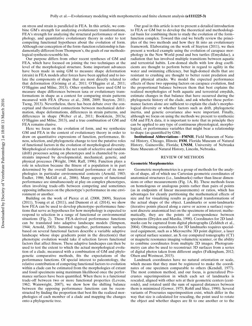
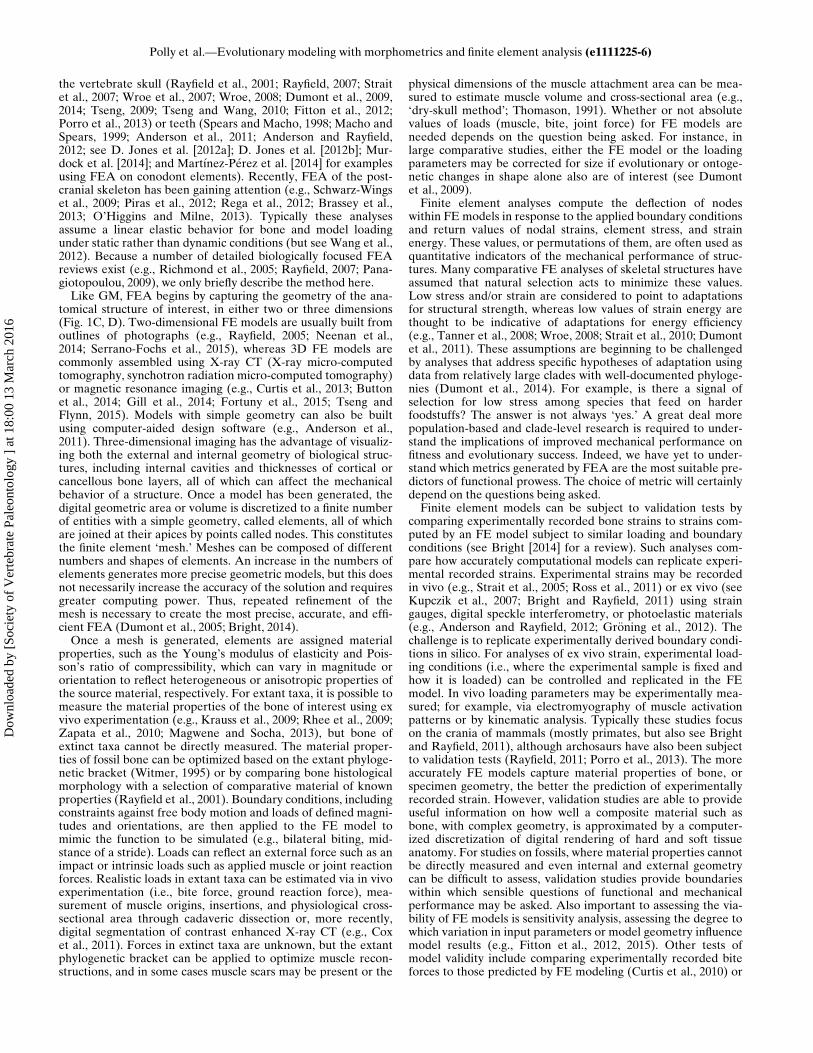
FIGURE 1. Illustrations of steps in the process of generating new FE models from landmark data and an existing FE model. Anterior is to the rightfor all figures. A, landmark data for a ‘base’ FE model (shown in C). Black lines illustrate features of the corresponding shell; gray lines show a gridassociated with the landmark coordinates; B, landmark data from another specimen of interest. Again, black lines indicate shell features; gray linesshow the deformation required to transform the ‘base’ model coordinates into the new coordinates, as interpolated by a thin-plate spline function.Note that in this case, the two-dimensional visualization is for representational purposes only and does not fully describe the shape differencesbetween the turtle shells in three dimensions. See Klingenberg (2013) for more information on visualizations in geometric morphometrics; C, the‘base’ FE model; D, a new FE model generated by applying the thin-plate spline interpolation function to the coordinates of all nodes in the ‘base’model; E, stresses resulting from the application of an anterior midline load to the new FE model. Warmer colors indicate high stresses; cooler colorsindicate low stresses.

Polly et al.—Evolutionary modeling with morphometrics and finite element analysis (e1111225-2)

Dow

nloa

ded

by [

Soci

ety

of V

erte

brat

e Pa

leon

tolo

gy ]

at 1

8:00

13

Mar

ch 2

016

on stress and strain is paralleled in FEA. In this article, we com-bine GM’s strength for analyzing evolutionary transformations,FEA’s strength for analyzing the structural performance of mor-phology, and quantitative evolutionary theory in order to testcompeting functional hypotheses about the evolution of form.Although our conception of the form–function relationship is fun-damentally different fromThompson’s, the goals of our methodo-logical synthesis resemble his.Our purpose differs from other recent syntheses of GM and

FEA, which have focused on joining the two techniques at thelevel of the morphological structure. Some important advanceshave been made in using GM to measure shape deformation(strain) in FEA models after forces have been applied and to iso-late the components of shape that are most directly related tothat deformation (Gr€oning et al., 2011; O’Higgins et al., 2011;O’Higgins and Milne, 2013). Other syntheses have used GM tomeasure shape differences between taxa or evolutionary trans-formations in shape as a context for comparing strain patternsmeasured with FEA (Pierce et al., 2008, 2009; Stayton, 2011;Tseng, 2013). Nevertheless, there has been debate over the con-ceptual and theoretical connections between mechanical defor-mation, shape deformations, differences in strain patterns, anddifferences in shape (Weber et al., 2011; Bookstein, 2013a;O’Higgins and Milne, 2013), and a true combination of GM andFEA remains elusive.Here we focus on the evolution of form, and we synthesize

GM and FEA in the context of evolutionary theory in order todraw on quantitative expressions of function, performance, fit-ness, selection, and phylogenetic change to test the putative rolesof functional factors in the evolution of morphological diversity.Morphological evolution is the net result of selective and random(drift) processes acting on phenotypes and is channeled by con-straints imposed by developmental, mechanical, genetic, andphysical processes (Wright, 1968; Raff, 1996). Function plays arole in selection because the fitness of a population is in partdetermined by the overall functional performance of its mor-phologies in particular environmental contexts (Arnold, 1983;Endler, 1986; McGill et al., 2006). Many aspects of functionalperformance are simultaneously at play on complex phenotypes,often involving trade-offs between competing and sometimesopposing influences on the phenotype’s performance in one envi-ronment or another.Building on the work of Pierce et al. (2008, 2009), Stayton

(2011), Young et al. (2011), and Dumont et al. (2014), we showhow FEA can be used to develop phenotype–performance func-tions that serve as hypotheses for how morphology is expected torespond to selection in a range of functional or environmentalsituations (Fig. 2). These FEA-derived performance functionscan be translated into adaptive landscape models (Simpson,1944; Arnold, 2003). Summed together, performance surfacesbased on several functional factors describe a variable adaptivelandscape whose slope gradients point in the direction(s) thatphenotypic evolution would take if selection favors functionalfactors that affect fitness. These adaptive landscapes can then beused to test the extent to which the actual morphological evolu-tion of a clade, measured with a combination of GM and phylo-genetic comparative methods, fits the expectations of theperformance functions. Of special interest to paleontology, therelative contribution of competing functional factors to evolutionwithin a clade can be estimated from the morphologies of extantand fossil specimens using maximum likelihood once the perfor-mance surfaces have been quantified. When there is a functionaltrade-off between two or more functional properties (Levens,1962; Wainwright, 2007), we show how the shifting balancebetween the opposing performance functions can be recon-structed by finding the proportion that best fits the realized mor-phologies of each member of a clade and mapping the changesonto a phylogenetic tree.

Our goal in this article is not to present a detailed introductionto FEA or GM but to develop the theoretical and methodologi-cal basis for combining them to study the evolution of the form–function complex. Toward this end we briefly review the princi-ples of the two methods and how they fit into an evolutionaryframework. Elaborating on the work of Stayton (2011), we thenpresent a worked example using the evolution of carapace mor-phology in the New World pond and box turtles (Emydidae), aradiation that has involved multiple transitions between aquaticand terrestrial habits. Low-domed shells with low drag coeffi-cients are thought to perform better in regard to agility in thewater and swimming efficiency, but high-domed shells that areresistant to crushing are thought to better resist predation andother physical attacks. We model the expected performanceeffects of these two opposing factors on carapace evolution, findthe proportional balance between them that best explains therealized morphologies of both aquatic and terrestrial emydids,estimate changes in that balance that have occurred during thephylogenetic history of the clade, and ask whether these perfor-mance factors alone are sufficient to explain the clade’s morpho-logical diversity or whether factors such as drift, phylogeneticinertia, and genetic covariance also were important. Finally,although we focus on using the methods we present to synthesizeGM and FEA data, it is important to note that in principle theycan be applied to any type of continuous physiological, morpho-logical, or performance variables that might bear a relationshipto shape (as quantified by GM).Institutional Abbreviations—FMNH, Field Museum of Natu-

ral History, Chicago, Illinois; FSM, Florida Museum of NaturalHistory, Gainesville, Florida; UNSM, University of NebraskaState Museum of Natural History, Lincoln, Nebraska.

REVIEWOFMETHODS

Geometric Morphometrics

Geometric morphometrics is a group of methods for the analy-sis of shape, all of which use Cartesian geometric coordinates ofanatomical structures (i.e., landmarks) rather than linear dimen-sions or other measurements (Fig. 1A, B). These methods focuson homologous or analogous points rather than pairs of points(as in endpoints of linear measurements) or ratios, which hasadvantages for cleanly partitioning the mathematical effects ofsize and for visualizing results as graphical transformations ofthe actual shape of the object. Landmarks or semi-landmarks(iterative points placed along a curve or across a surface) repre-sent discrete anatomical loci on the specimens of interest; mathe-matically, they are the points of correspondence betweenspecimens (Dryden and Mardia, 1998). Coordinates for 2D land-marks can be captured from digital photographs (Zelditch et al.,2004). Obtaining coordinates for 3D landmarks requires special-ized equipment, such as a Microscribe 3D point digitizer, a laseror optical surface scanner, an X-ray computed tomography (CT)or magnetic resonance imaging volumetric scanner, or the abilityto combine coordinates from multiple 2D images. Photogram-metry can also be used to reconstruct 3D surfaces from a seriesof digital photos taken from different angles (Falkingham, 2012;Olsen and Westneat, 2015).Landmark coordinates have no natural orientation or scale,

which means that they must be registered to make the coordi-nates of one specimen comparable to others (Kendall, 1977).The most common method, and our focus, is generalized Pro-crustes superimposition in which each set of landmarks isrescaled, aligned with other sets at their geometric centers (cent-roids), and rotated until the sum of squared distances betweenthem is minimized (Gower, 1975; Rohlf and Slice, 1990). Severalvariants of Procrustes superimposition exist, which differ in theway that size is calculated for rescaling, the point used to rotatethe object and whether shapes are fit to one another or to the


Dow

nloa

ded

by [

Soci

ety

of V

erte

brat

e Pa

leon

tolo

gy ]

at 1

8:00

13

Mar

ch 2

016

sample mean (see reviews in Zelditch et al., 2004; Slice, 2005).The removal of size, orientation, and translation reduce thedegrees of freedom of the Procrustes aligned coordinates (loss of4 degrees of freedom for 2D landmarks and 7 for 3D landmarks).The reduced dimensionality constrains variation such that shapesare distributed in a non-Euclidean mathematical space with theform of a hyperdimensional sphere or hemisphere (Kendall,1984, 1985; Dryden and Mardia, 1998; Slice, 2001). Because ofthe non-Euclidean geometry of shape space, Procrustes coordi-nates are usually projected to a Euclidean tangent space,although in practice this is often unnecessary for biologicalshapes because developmental and functional integration

typically constrains shape variation sufficiently that the non-Euclidean curvatures of shape space are inconsequential (Rohlfand Slice, 1990; Rohlf, 1999; Slice, 2001).The Procrustes superimposed coordinates are the entry

point for many multivariate analyses of shape. The coordi-nates themselves may be used as shape variables, but theircovariances and reduced degrees of freedom must be takeninto account when calculating p-values or other statistics.More commonly the coordinates are converted into one oftwo types of shape variables so that they have the propernumber of degrees of freedom. The first method is to factorthe coordinates into partial warp and uniform component

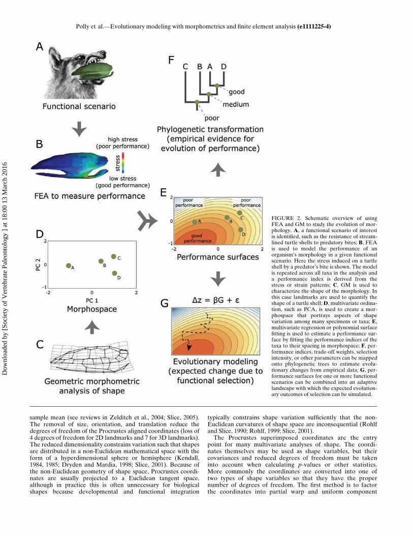
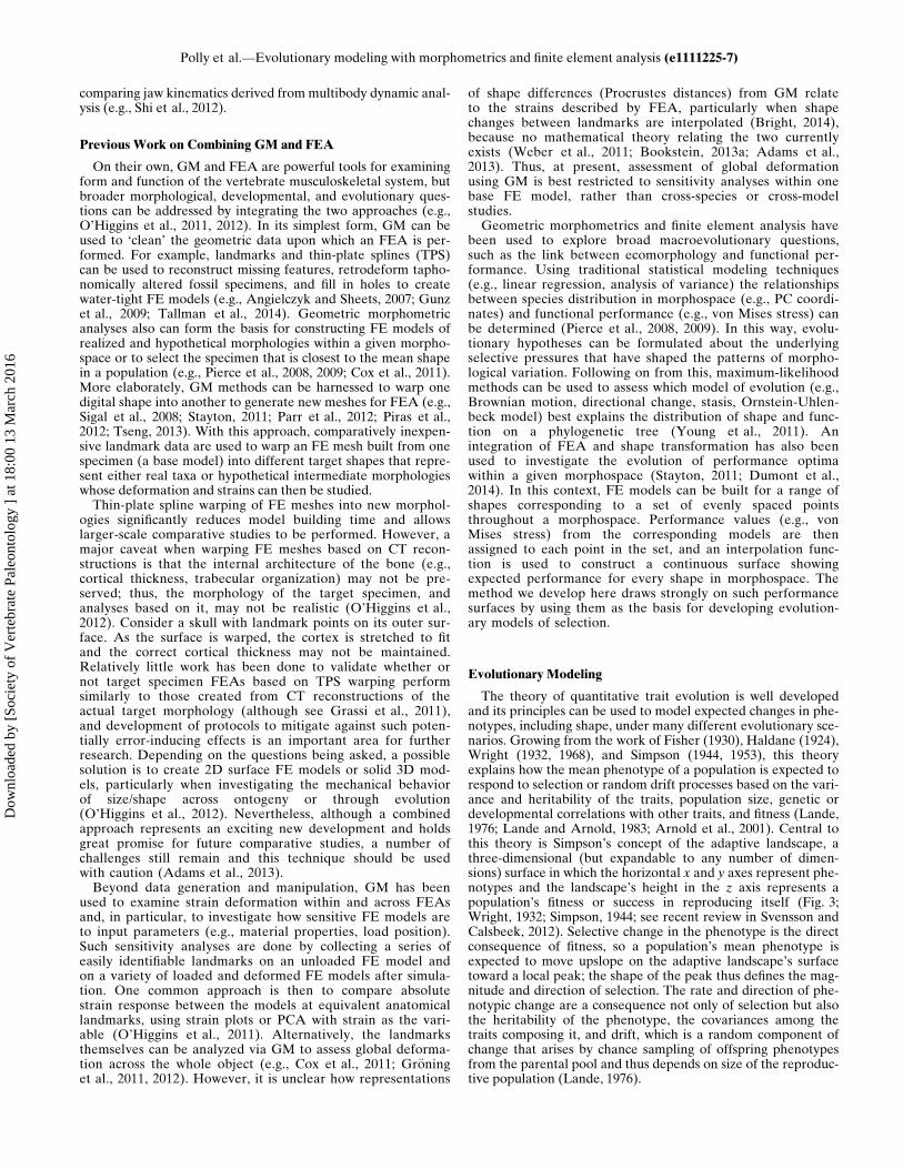
FIGURE 2. Schematic overview of usingFEA and GM to study the evolution of mor-phology. A, a functional scenario of interestis identified, such as the resistance of stream-lined turtle shells to predatory bites; B, FEAis used to model the performance of anorganism’s morphology in a given functionalscenario. Here the stress induced on a turtleshell by a predator’s bite is shown. The modelis repeated across all taxa in the analysis anda performance index is derived from thestress or strain patterns; C, GM is used tocharacterize the shape of the morphology. Inthis case landmarks are used to quantify theshape of a turtle shell;D, multivariate ordina-tion, such as PCA, is used to create a mor-phospace that portrays aspects of shapevariation among many specimens or taxa; E,multivariate regression or polynomial surfacefitting is used to estimate a performance sur-face by fitting the performance indices of thetaxa to their spacing in morphospace; F, per-formance indices, trade-off weights, selectionintensity, or other parameters can be mappedonto phylogenetic trees to estimate evolu-tionary changes from empirical data; G, per-formance surfaces for one or more functionalscenarios can be combined into an adaptivelandscape with which the expected evolution-ary outcomes of selection can be simulated.


Dow

nloa

ded

by [

Soci

ety

of V

erte

brat

e Pa

leon

tolo

gy ]

at 1

8:00

13

Mar

ch 2

016

scores using a thin-plate spline decomposition (Bookstein,1989, 1991; Rohlf, 1995; Zelditch et al., 2004). Each dimen-sion of warp scores captures shape variation on different spa-tial scales. These scores have the correct number of degreesof freedom, but the different scales are still intercorrelated.The second and more common method of producing shapescores is to project the Procrustes coordinates onto their prin-cipal component (PC) axes (eigenvectors; Rohlf, 1993; Dry-den and Mardia, 1998). Each dimension of PC shaperepresents a module of correlated variation in landmark coor-dinates that is orthogonal to other dimensions. Scores of theobjects on the PC axes are shape variables that have boththe proper number of degrees of freedom and are uncorre-lated. Note that principal component decomposition of thepartial warp and uniform component scores, known as rela-tive warps analysis, produces identical shape variables solong as all the partial and uniform components are weightedequally (Rohlf, 1993). Standard multivariate statistical proce-dures such as multivariate regression and multivariate analy-sis of variance can be performed on the shape variables, butnonparametric permutation-based tests are recommendedover traditional tests based on parametric F-distributions orWilks’ lambda because shape variation seldom meets therequired assumptions of normality and sample sizes are sel-dom balanced (Manly, 1991; Zelditch et al., 2004; Mitter-oecker and Gunz, 2009; Kowalewski and Novack-Gottshall,2010). Nonparametric Procrustes analysis of variance testsbased on multivariate distance between objects rather thanon shape variables are also available (Klingenberg and McIn-tyre, 1998; Klingenberg, 2015).The thin-plate spline can be used as a device for visualizing

shape differences, decomposing shape variation by spatial scale,and (of particular interest for this study) morphing one digitalobject into the form of another using landmarks as tie points(Fig. 1; Bookstein, 1989). A spline function is fit to the displace-ments of landmarks caused by transforming a reference shapeinto a target shape and is used to interpolate the displacement ofpoints that lie between the object’s landmarks. The spline func-tion is frequently used to deform a square grid placed on the ref-erence object into a D’Arcy Thompson-like diagram of theshape transformation. The thin-plate spline also can be used todecompose shape differences into geometric components. Theuniform (or affine) component describes shape differences thataffect a target specimen equally across the whole specimen,whereas the nonuniform component describes localized shapedifferences (e.g., Bookstein, 1989, 1991, 1996b). Thin-plate splinevisualizations are usually used with two-dimensional data, butthey also can be applied to three-dimensional shapes (Bookstein,1996b; Rohlf and Bookstein, 2003). Importantly, thin-platesplines can be used to transform larger grids or blocks of coordi-nate data based on a selected set of homologous landmarks(Bookstein, 1991; Zelditch et al., 2004; Wiley et al., 2005). Thespline functions are fit to either two- or three-dimensional land-marks that have been placed on more complete digital objects,such as a photograph or 3D scan. The spline functions are thenused to interpolate all the data points from the reference to thetarget object. Stayton (2009) showed how this procedure couldbe used to morph a reference FEA model into the forms of sev-eral target specimens, alleviating the need for an independentoriginal scan of each specimen.Important for our own analysis, principal component analysis

(PCA) of Procrustes coordinates also produces a multivariateshape space, or morphospace (Fig. 2; Rohlf, 1993; Mardia andDryden, 1998; Mitteroecker and Huttegger, 2009). Each point inmorphospace represents a unique shape and each axis of thespace represents an aspect of shape variation that is mathemati-cally independent of variation on other axes. The distribution ofreal objects in morphospace is based on their shape similarity,

the distances between them being identical to their Procrustesshape distances (the summed distances between correspondinglandmarks) in the non-Euclidean geometry of shape space. Notethat when shapes belonging to a time series, such as an ontoge-netic series, evolutionary lineage, or serially repeated structures,are projected into PC space, the trajectory connecting them canbe highly nonlinear (Mitteroecker et al., 2004; Adams andCollyer, 2009; Collyer and Adams, 2013), forming predictablecurves that describe increasingly smaller subdivisions of theentire series (Bookstein, 2013b). Multivariate regression ofshape onto continuous independent factors such as body size,age, stress for a given load, or fitness yields prediction equationsthat can be visualized as lines, contour maps, surfaces, or hyper-dimensional surfaces within the morphospace. In this article wevisualize the relationship between shell shape and its functionalproperties by using such surfaces, whose contours show the path-ways that shape evolution is expected to take if it is influencedby those functional factors.Readers interested in Procrustes-based shape analysis can

refer to recent reviews of the history of the technique (Book-stein, 1996a; 1998; Adams et al., 2004; Slice, 2005), associatedanalytical methodologies (Rohlf and Marcus, 1993;O’Higgins, 2000; Mitteroecker and Gunz, 2009; Klingenberg,2013; Bookstein, 2014), and practical applications (Slice,2007; Klingenberg, 2010; Lawing and Polly, 2010; Adamset al., 2013). Several book-length introductions to methodsand theory are also available (Dryden and Mardia, 1998;Claude, 2008; Weber and Bookstein, 2011; Zelditch et al.,2004, 2012). Procrustes-based analysis can also be carried outon curves and surfaces using semi-landmarks (Bookstein,1991, 1997; Gunz et al., 2005). Different methods exist forsuperimposing semi-landmarks, based on minimizing distan-ces between individuals and the reference form (Sampsonet al., 1996) or minimizing the bending energy of the thin-plate spline describing the difference between a specimenand the reference form (Green, 1996; Bookstein, 1997), withminor implications for the statistical properties of the super-imposed data (see review in Zelditch et al., 2012).Geometric morphometrics has become a standard tool in ver-

tebrate paleontology. Recent examples of its application includestudies of developmental patterns and mechanisms (B€ohmeret al., 2015; Bhullar et al., 2015; Head and Polly, 2015), morpho-logical integration (Goswami et al., 2015), intraspecific variationand sexual dimorphism (Cullen et al., 2014; Drake et al., 2015),taxonomy and phylogenetics (Abdala et al., 2014; Geraads, 2014;Benoit et al., 2015; Sansalone et al., 2015), functional morphol-ogy (Fabre et al., 2014; Mart�ın-Serra et al., 2014; Fearon andVarricchio, 2015; Piras et al., 2015), responses to climate change(Meachen et al., 2014; O’Keefe et al., 2014), paleoecology (K. E.Jones et al., 2014; Mallon and Anderson, 2014; Dieleman et al.,2015; Meloro et al., 2015), and ichnology (Castanera et al., 2015;Ledoux and Boudadi-Maligne, 2015), as well as advances in mor-phometric methodology (Arbour and Brown, 2014; Hethering-ton et al., 2015).

Finite Element Analysis

Finite element analysis is a computational technique thatinvokes the mathematical principles of the finite element methodto predict the behavior of a structure with defined material prop-erties in response to user-determined loads and constraints. Thetechnique is commonplace in engineering analysis (see review ofits early development in Clough, 1990) and has been used exten-sively in orthopedic medicine and implant studies for a numberof decades (Zienkiewicz et al., 1983). Since the early 2000s, FEAhas gained traction as a technique for studying the mechanicalbehavior and performance of extinct and extant organisms, mostcommonly vertebrates, with particular emphasis on studies of


Dow

nloa

ded

by [

Soci

ety

of V

erte

brat

e Pa

leon

tolo

gy ]

at 1

8:00

13

Mar

ch 2

016

the vertebrate skull (Rayfield et al., 2001; Rayfield, 2007; Straitet al., 2007; Wroe et al., 2007; Wroe, 2008; Dumont et al., 2009,2014; Tseng, 2009; Tseng and Wang, 2010; Fitton et al., 2012;Porro et al., 2013) or teeth (Spears and Macho, 1998; Macho andSpears, 1999; Anderson et al., 2011; Anderson and Rayfield,2012; see D. Jones et al. [2012a]; D. Jones et al. [2012b]; Mur-dock et al. [2014]; and Mart�ınez-P�erez et al. [2014] for examplesusing FEA on conodont elements). Recently, FEA of the post-cranial skeleton has been gaining attention (e.g., Schwarz-Wingset al., 2009; Piras et al., 2012; Rega et al., 2012; Brassey et al.,2013; O’Higgins and Milne, 2013). Typically these analysesassume a linear elastic behavior for bone and model loadingunder static rather than dynamic conditions (but see Wang et al.,2012). Because a number of detailed biologically focused FEAreviews exist (e.g., Richmond et al., 2005; Rayfield, 2007; Pana-giotopoulou, 2009), we only briefly describe the method here.Like GM, FEA begins by capturing the geometry of the ana-

tomical structure of interest, in either two or three dimensions(Fig. 1C, D). Two-dimensional FE models are usually built fromoutlines of photographs (e.g., Rayfield, 2005; Neenan et al.,2014; Serrano-Fochs et al., 2015), whereas 3D FE models arecommonly assembled using X-ray CT (X-ray micro-computedtomography, synchotron radiation micro-computed tomography)or magnetic resonance imaging (e.g., Curtis et al., 2013; Buttonet al., 2014; Gill et al., 2014; Fortuny et al., 2015; Tseng andFlynn, 2015). Models with simple geometry can also be builtusing computer-aided design software (e.g., Anderson et al.,2011). Three-dimensional imaging has the advantage of visualiz-ing both the external and internal geometry of biological struc-tures, including internal cavities and thicknesses of cortical orcancellous bone layers, all of which can affect the mechanicalbehavior of a structure. Once a model has been generated, thedigital geometric area or volume is discretized to a finite numberof entities with a simple geometry, called elements, all of whichare joined at their apices by points called nodes. This constitutesthe finite element ‘mesh.’ Meshes can be composed of differentnumbers and shapes of elements. An increase in the numbers ofelements generates more precise geometric models, but this doesnot necessarily increase the accuracy of the solution and requiresgreater computing power. Thus, repeated refinement of themesh is necessary to create the most precise, accurate, and effi-cient FEA (Dumont et al., 2005; Bright, 2014).Once a mesh is generated, elements are assigned material

properties, such as the Young’s modulus of elasticity and Pois-son’s ratio of compressibility, which can vary in magnitude ororientation to reflect heterogeneous or anisotropic properties ofthe source material, respectively. For extant taxa, it is possible tomeasure the material properties of the bone of interest using exvivo experimentation (e.g., Krauss et al., 2009; Rhee et al., 2009;Zapata et al., 2010; Magwene and Socha, 2013), but bone ofextinct taxa cannot be directly measured. The material proper-ties of fossil bone can be optimized based on the extant phyloge-netic bracket (Witmer, 1995) or by comparing bone histologicalmorphology with a selection of comparative material of knownproperties (Rayfield et al., 2001). Boundary conditions, includingconstraints against free body motion and loads of defined magni-tudes and orientations, are then applied to the FE model tomimic the function to be simulated (e.g., bilateral biting, mid-stance of a stride). Loads can reflect an external force such as animpact or intrinsic loads such as applied muscle or joint reactionforces. Realistic loads in extant taxa can be estimated via in vivoexperimentation (i.e., bite force, ground reaction force), mea-surement of muscle origins, insertions, and physiological cross-sectional area through cadaveric dissection or, more recently,digital segmentation of contrast enhanced X-ray CT (e.g., Coxet al., 2011). Forces in extinct taxa are unknown, but the extantphylogenetic bracket can be applied to optimize muscle recon-structions, and in some cases muscle scars may be present or the

physical dimensions of the muscle attachment area can be mea-sured to estimate muscle volume and cross-sectional area (e.g.,‘dry-skull method’; Thomason, 1991). Whether or not absolutevalues of loads (muscle, bite, joint force) for FE models areneeded depends on the question being asked. For instance, inlarge comparative studies, either the FE model or the loadingparameters may be corrected for size if evolutionary or ontoge-netic changes in shape alone also are of interest (see Dumontet al., 2009).Finite element analyses compute the deflection of nodes

within FE models in response to the applied boundary conditionsand return values of nodal strains, element stress, and strainenergy. These values, or permutations of them, are often used asquantitative indicators of the mechanical performance of struc-tures. Many comparative FE analyses of skeletal structures haveassumed that natural selection acts to minimize these values.Low stress and/or strain are considered to point to adaptationsfor structural strength, whereas low values of strain energy arethought to be indicative of adaptations for energy efficiency(e.g., Tanner et al., 2008; Wroe, 2008; Strait et al., 2010; Dumontet al., 2011). These assumptions are beginning to be challengedby analyses that address specific hypotheses of adaptation usingdata from relatively large clades with well-documented phyloge-nies (Dumont et al., 2014). For example, is there a signal ofselection for low stress among species that feed on harderfoodstuffs? The answer is not always ‘yes.’ A great deal morepopulation-based and clade-level research is required to under-stand the implications of improved mechanical performance onfitness and evolutionary success. Indeed, we have yet to under-stand which metrics generated by FEA are the most suitable pre-dictors of functional prowess. The choice of metric will certainlydepend on the questions being asked.Finite element models can be subject to validation tests by

comparing experimentally recorded bone strains to strains com-puted by an FE model subject to similar loading and boundaryconditions (see Bright [2014] for a review). Such analyses com-pare how accurately computational models can replicate experi-mental recorded strains. Experimental strains may be recordedin vivo (e.g., Strait et al., 2005; Ross et al., 2011) or ex vivo (seeKupczik et al., 2007; Bright and Rayfield, 2011) using straingauges, digital speckle interferometry, or photoelastic materials(e.g., Anderson and Rayfield, 2012; Gr€oning et al., 2012). Thechallenge is to replicate experimentally derived boundary condi-tions in silico. For analyses of ex vivo strain, experimental load-ing conditions (i.e., where the experimental sample is fixed andhow it is loaded) can be controlled and replicated in the FEmodel. In vivo loading parameters may be experimentally mea-sured; for example, via electromyography of muscle activationpatterns or by kinematic analysis. Typically these studies focuson the crania of mammals (mostly primates, but also see Brightand Rayfield, 2011), although archosaurs have also been subjectto validation tests (Rayfield, 2011; Porro et al., 2013). The moreaccurately FE models capture material properties of bone, orspecimen geometry, the better the prediction of experimentallyrecorded strain. However, validation studies are able to provideuseful information on how well a composite material such asbone, with complex geometry, is approximated by a computer-ized discretization of digital rendering of hard and soft tissueanatomy. For studies on fossils, where material properties cannotbe directly measured and even internal and external geometrycan be difficult to assess, validation studies provide boundarieswithin which sensible questions of functional and mechanicalperformance may be asked. Also important to assessing the via-bility of FE models is sensitivity analysis, assessing the degree towhich variation in input parameters or model geometry influencemodel results (e.g., Fitton et al., 2012, 2015). Other tests ofmodel validity include comparing experimentally recorded biteforces to those predicted by FE modeling (Curtis et al., 2010) or


Dow

nloa

ded

by [

Soci

ety

of V

erte

brat

e Pa

leon

tolo

gy ]

at 1

8:00

13

Mar

ch 2

016

comparing jaw kinematics derived from multibody dynamic anal-ysis (e.g., Shi et al., 2012).

Previous Work on Combining GM and FEA

On their own, GM and FEA are powerful tools for examiningform and function of the vertebrate musculoskeletal system, butbroader morphological, developmental, and evolutionary ques-tions can be addressed by integrating the two approaches (e.g.,O’Higgins et al., 2011, 2012). In its simplest form, GM can beused to ‘clean’ the geometric data upon which an FEA is per-formed. For example, landmarks and thin-plate splines (TPS)can be used to reconstruct missing features, retrodeform tapho-nomically altered fossil specimens, and fill in holes to createwater-tight FE models (e.g., Angielczyk and Sheets, 2007; Gunzet al., 2009; Tallman et al., 2014). Geometric morphometricanalyses also can form the basis for constructing FE models ofrealized and hypothetical morphologies within a given morpho-space or to select the specimen that is closest to the mean shapein a population (e.g., Pierce et al., 2008, 2009; Cox et al., 2011).More elaborately, GM methods can be harnessed to warp onedigital shape into another to generate new meshes for FEA (e.g.,Sigal et al., 2008; Stayton, 2011; Parr et al., 2012; Piras et al.,2012; Tseng, 2013). With this approach, comparatively inexpen-sive landmark data are used to warp an FE mesh built from onespecimen (a base model) into different target shapes that repre-sent either real taxa or hypothetical intermediate morphologieswhose deformation and strains can then be studied.Thin-plate spline warping of FE meshes into new morphol-

ogies significantly reduces model building time and allowslarger-scale comparative studies to be performed. However, amajor caveat when warping FE meshes based on CT recon-structions is that the internal architecture of the bone (e.g.,cortical thickness, trabecular organization) may not be pre-served; thus, the morphology of the target specimen, andanalyses based on it, may not be realistic (O’Higgins et al.,2012). Consider a skull with landmark points on its outer sur-face. As the surface is warped, the cortex is stretched to fitand the correct cortical thickness may not be maintained.Relatively little work has been done to validate whether ornot target specimen FEAs based on TPS warping performsimilarly to those created from CT reconstructions of theactual target morphology (although see Grassi et al., 2011),and development of protocols to mitigate against such poten-tially error-inducing effects is an important area for furtherresearch. Depending on the questions being asked, a possiblesolution is to create 2D surface FE models or solid 3D mod-els, particularly when investigating the mechanical behaviorof size/shape across ontogeny or through evolution(O’Higgins et al., 2012). Nevertheless, although a combinedapproach represents an exciting new development and holdsgreat promise for future comparative studies, a number ofchallenges still remain and this technique should be usedwith caution (Adams et al., 2013).Beyond data generation and manipulation, GM has been

used to examine strain deformation within and across FEAsand, in particular, to investigate how sensitive FE models areto input parameters (e.g., material properties, load position).Such sensitivity analyses are done by collecting a series ofeasily identifiable landmarks on an unloaded FE model andon a variety of loaded and deformed FE models after simula-tion. One common approach is then to compare absolutestrain response between the models at equivalent anatomicallandmarks, using strain plots or PCA with strain as the vari-able (O’Higgins et al., 2011). Alternatively, the landmarksthemselves can be analyzed via GM to assess global deforma-tion across the whole object (e.g., Cox et al., 2011; Gr€oninget al., 2011, 2012). However, it is unclear how representations

of shape differences (Procrustes distances) from GM relateto the strains described by FEA, particularly when shapechanges between landmarks are interpolated (Bright, 2014),because no mathematical theory relating the two currentlyexists (Weber et al., 2011; Bookstein, 2013a; Adams et al.,2013). Thus, at present, assessment of global deformationusing GM is best restricted to sensitivity analyses within onebase FE model, rather than cross-species or cross-modelstudies.Geometric morphometrics and finite element analysis have

been used to explore broad macroevolutionary questions,such as the link between ecomorphology and functional per-formance. Using traditional statistical modeling techniques(e.g., linear regression, analysis of variance) the relationshipsbetween species distribution in morphospace (e.g., PC coordi-nates) and functional performance (e.g., von Mises stress) canbe determined (Pierce et al., 2008, 2009). In this way, evolu-tionary hypotheses can be formulated about the underlyingselective pressures that have shaped the patterns of morpho-logical variation. Following on from this, maximum-likelihoodmethods can be used to assess which model of evolution (e.g.,Brownian motion, directional change, stasis, Ornstein-Uhlen-beck model) best explains the distribution of shape and func-tion on a phylogenetic tree (Young et al., 2011). Anintegration of FEA and shape transformation has also beenused to investigate the evolution of performance optimawithin a given morphospace (Stayton, 2011; Dumont et al.,2014). In this context, FE models can be built for a range ofshapes corresponding to a set of evenly spaced pointsthroughout a morphospace. Performance values (e.g., vonMises stress) from the corresponding models are thenassigned to each point in the set, and an interpolation func-tion is used to construct a continuous surface showingexpected performance for every shape in morphospace. Themethod we develop here draws strongly on such performancesurfaces by using them as the basis for developing evolution-ary models of selection.

Evolutionary Modeling

The theory of quantitative trait evolution is well developedand its principles can be used to model expected changes in phe-notypes, including shape, under many different evolutionary sce-narios. Growing from the work of Fisher (1930), Haldane (1924),Wright (1932, 1968), and Simpson (1944, 1953), this theoryexplains how the mean phenotype of a population is expected torespond to selection or random drift processes based on the vari-ance and heritability of the traits, population size, genetic ordevelopmental correlations with other traits, and fitness (Lande,1976; Lande and Arnold, 1983; Arnold et al., 2001). Central tothis theory is Simpson’s concept of the adaptive landscape, athree-dimensional (but expandable to any number of dimen-sions) surface in which the horizontal x and y axes represent phe-notypes and the landscape’s height in the z axis represents apopulation’s fitness or success in reproducing itself (Fig. 3;Wright, 1932; Simpson, 1944; see recent review in Svensson andCalsbeek, 2012). Selective change in the phenotype is the directconsequence of fitness, so a population’s mean phenotype isexpected to move upslope on the adaptive landscape’s surfacetoward a local peak; the shape of the peak thus defines the mag-nitude and direction of selection. The rate and direction of phe-notypic change are a consequence not only of selection but alsothe heritability of the phenotype, the covariances among thetraits composing it, and drift, which is a random component ofchange that arises by chance sampling of offspring phenotypesfrom the parental pool and thus depends on size of the reproduc-tive population (Lande, 1976).


Dow

nloa

ded

by [

Soci

ety

of V

erte

brat

e Pa

leon

tolo

gy ]

at 1

8:00

13

Mar

ch 2

016

Evolutionary change in the average phenotype of a species(Dz) on an adaptive landscape (Arnold et al., 2001) can bedescribed as

DzDGbCG/N ; (1)

where G is the genetic covariance matrix, which is the heritablecomponent of the phenotypic variances of two or more traits; Nis the reproductive population size (G/N is the amount of changeby genetic drift); and b is the vector of selection gradientsdefined by the slope of the adaptive landscape surface W evalu-ated at the trait mean:

bD @lnW

@z: (2)

If N or b is large, then drift becomes a negligible component ofchange and the second term of Eq. (1) can be ignored (Fig. 3).Evolutionary patterns that emerge on a topographically com-

plex and changing adaptive landscape can be varied and multi-faceted, but they can often be classified into one of threestereotypical modes of evolution: stabilizing processes (includingstasis or Ornstein-Uhlenbeck processes), directional evolution,and Brownian motion (random change; Bookstein, 1987; McKin-ney, 1990; Gingerich, 1993; Hunt, 2006). The classic adaptivepeak model of evolution is an example of a stabilizing processbecause the selection gradients on the slopes point upward, drop-ping to zero at the top of the peak (Fig. 3). The adaptive peakthus carries the mean phenotypes in populations from their posi-tions on the slopes to a stable point at the peak. Once the peakhas been attained, evolutionary change ceases until external

forces provide opportunities for selection to come into play onceagain. The paths often follow curved trajectories that are definedby the direction of the selection gradient vectors, which are inturn defined by the curvature of the adaptive landscape (Fig. 3;Supplementary Data Movie 1). Directional selection is either ashort-lived phenomenon that occurs while the phenotype isbeing selected toward the peak or it is driven by an adaptivepeak whose optimum is changing in a uniform direction. Brow-nian motion corresponds to random change, which can be gener-ated by several distinct processes. Neutral drift, also known asgenetic drift, is a Brownian motion process that occurs by chancesampling of one generation from the previous and is a functionof population size (small populations are more prone to driftthan large ones). Randomly changing directional selection canalso produce a Brownian motion pattern, a process known asselective drift (Kimura, 1954). These two processes can be distin-guished by estimating the rate of evolutionary change. The rateof true drift should be small, equal to the heritable component ofthe population-level phenotypic variance divided by the breed-ing population size, whereas selective drift may be much faster(Lande, 1976; Polly, 2004). For animated examples of pheno-types evolving under each of these three modes using geometricmorphometrics, see Polly (2004).If evolution occurs according to one of these three simple

modes, the outcomes are statistically predictable if parameterssuch as the rate of change at each step in the evolutionary pro-cess, the phenotypic variances of the populations, the heritabil-ity, and the shape of the adaptive surface are known. UnderBrownian motion, for example, the average outcome of a singleevolving lineage will have the same phenotypic mean as theancestor and a variance equal to the squared step rate (step vari-ance) times the number of temporal steps (Raup, 1977;

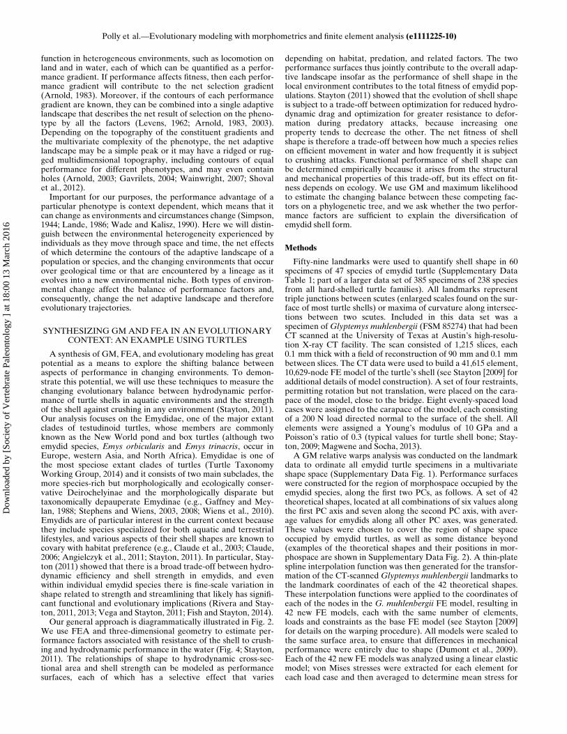
FIGURE 3. Evolution on an adaptive peak for a bivariate quantitative morphological trait, defined here as the first two principal components of tur-tle shell shape (x and y axes). Orange is the area of highest fitness and blue is the area of lowest fitness. Arrows show the direction and strength ofselection defined by the gradient of the landscape’s surface (Eq. (2)). Evolutionary pathways are shown in black. Stars mark the starting points; blackdots mark the peaks. Evolutionary change occurs by selection plus drift (Eq. (1)).A, when the drift component is zero, selection moves the phenotypedirectly to the peak following the contours defined by the selection gradients; B, when drift is small relative to the selection gradients, the phenotypeclimbs erratically to the peak and wanders around it in close proximity; C, when drift is equal in magnitude to selection, the phenotype wanders widelyaround the peak.


Dow

nloa

ded

by [

Soci

ety

of V

erte

brat

e Pa

leon

tolo

gy ]

at 1

8:00

13

Mar

ch 2

016

McKinney, 1990; Berg, 1993). On a phylogenetic tree, the sameoutcomes apply to each branch and the variance among the tiptaxa is a function of the squared step rate, the time since com-mon ancestry, and the covariances expected from the topologyof the tree (Felsenstein, 1988). These properties can be used toestimate the rate of trait evolution and the ancestral trait valuesat nodes within trees, or they can be used to remove confoundingeffects of phylogeny from statistical analyses of traits and inde-pendent factors (Felsenstein, 1988; Martins and Hansen, 1997).Each mode of evolution has known statistical properties, so thesame techniques can be applied to situations other than Brow-nian motion. In fact, rates, modes, and other parameters can beestimated from data on a phylogeny or within a single lineage by

finding the values that maximize the likelihood under each modeand then selecting the best mode using the Akaike informationcriterion or similar model selection criteria (Butler and King,2004; Hunt, 2006; Slater et al., 2011).Adaptive landscapes are often used to represent the fitness

effects of a single selective factor, but they can also be used torepresent the net outcome of many selective factors that affectthe phenotype (Arnold, 1983, 2003). Complex traits, such as theskeletal elements frequently preserved in the fossil record, per-form in more than one functional context and their net perfor-mance is a trade-off between competing demands (Fig. 4;Wainwright, 2007). Trade-offs may involve fundamentally differ-ent functions, such as locomotion and prey capture, or the same

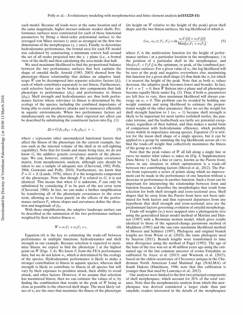
FIGURE 4. Performance surfaces definedby A, shell strength (resistance to crushing)and B, shell cross-sectional area, a compo-nent of hydrodynamic efficiency. Orange isthe area of strongest performance (greateststrength and smallest cross-sectional area,respectively) and blue is the area of weakestperformance. Arrows show selection gra-dients associated with optimization of eachfunction. Insets show optimal shell morpholo-gies; C, the adaptive landscape that resultsfrom combining the two surfaces, with selec-tion for hydrodynamic performance weighted0.2 relative to selection for shell strength andD, with hydrodynamic performance weighted1.2 relative to selection for shell strength.The selective optimum (black dot) alwayslies along the Pareto front. Note that theadaptive peak in Fig. 2 is the combination ofthe two performance surfaces weightedequally.


Dow

nloa

ded

by [

Soci

ety

of V

erte

brat

e Pa

leon

tolo

gy ]

at 1

8:00

13

Mar

ch 2

016

function in heterogeneous environments, such as locomotion onland and in water, each of which can be quantified as a perfor-mance gradient. If performance affects fitness, then each perfor-mance gradient will contribute to the net selection gradient(Arnold, 1983). Moreover, if the contours of each performancegradient are known, they can be combined into a single adaptivelandscape that describes the net result of selection on the pheno-type by all the factors (Levens, 1962; Arnold, 1983, 2003).Depending on the topography of the constituent gradients andthe multivariate complexity of the phenotype, the net adaptivelandscape may be a simple peak or it may have a ridged or rug-ged multidimensional topography, including contours of equalperformance for different phenotypes, and may even containholes (Arnold, 2003; Gavrilets, 2004; Wainwright, 2007; Shovalet al., 2012).Important for our purposes, the performance advantage of a

particular phenotype is context dependent, which means that itcan change as environments and circumstances change (Simpson,1944; Lande, 1986; Wade and Kalisz, 1990). Here we will distin-guish between the environmental heterogeneity experienced byindividuals as they move through space and time, the net effectsof which determine the contours of the adaptive landscape of apopulation or species, and the changing environments that occurover geological time or that are encountered by a lineage as itevolves into a new environmental niche. Both types of environ-mental change affect the balance of performance factors and,consequently, change the net adaptive landscape and thereforeevolutionary trajectories.

SYNTHESIZING GMAND FEA IN AN EVOLUTIONARYCONTEXT: AN EXAMPLE USING TURTLES

A synthesis of GM, FEA, and evolutionary modeling has greatpotential as a means to explore the shifting balance betweenaspects of performance in changing environments. To demon-strate this potential, we will use these techniques to measure thechanging evolutionary balance between hydrodynamic perfor-mance of turtle shells in aquatic environments and the strengthof the shell against crushing in any environment (Stayton, 2011).Our analysis focuses on the Emydidae, one of the major extantclades of testudinoid turtles, whose members are commonlyknown as the New World pond and box turtles (although twoemydid species, Emys orbicularis and Emys trinacris, occur inEurope, western Asia, and North Africa). Emydidae is one ofthe most speciose extant clades of turtles (Turtle TaxonomyWorking Group, 2014) and it consists of two main subclades, themore species-rich but morphologically and ecologically conser-vative Deirochelyinae and the morphologically disparate buttaxonomically depauperate Emydinae (e.g., Gaffney and Mey-lan, 1988; Stephens and Wiens, 2003, 2008; Wiens et al., 2010).Emydids are of particular interest in the current context becausethey include species specialized for both aquatic and terrestriallifestyles, and various aspects of their shell shapes are known tocovary with habitat preference (e.g., Claude et al., 2003; Claude,2006; Angielczyk et al., 2011; Stayton, 2011). In particular, Stay-ton (2011) showed that there is a broad trade-off between hydro-dynamic efficiency and shell strength in emydids, and evenwithin individual emydid species there is fine-scale variation inshape related to strength and streamlining that likely has signifi-cant functional and evolutionary implications (Rivera and Stay-ton, 2011, 2013; Vega and Stayton, 2011; Fish and Stayton, 2014).Our general approach is diagrammatically illustrated in Fig. 2.

We use FEA and three-dimensional geometry to estimate per-formance factors associated with resistance of the shell to crush-ing and hydrodynamic performance in the water (Fig. 4; Stayton,2011). The relationships of shape to hydrodynamic cross-sec-tional area and shell strength can be modeled as performancesurfaces, each of which has a selective effect that varies

depending on habitat, predation, and related factors. The twoperformance surfaces thus jointly contribute to the overall adap-tive landscape insofar as the performance of shell shape in thelocal environment contributes to the total fitness of emydid pop-ulations. Stayton (2011) showed that the evolution of shell shapeis subject to a trade-off between optimization for reduced hydro-dynamic drag and optimization for greater resistance to defor-mation during predatory attacks, because increasing oneproperty tends to decrease the other. The net fitness of shellshape is therefore a trade-off between how much a species relieson efficient movement in water and how frequently it is subjectto crushing attacks. Functional performance of shell shape canbe determined empirically because it arises from the structuraland mechanical properties of this trade-off, but its effect on fit-ness depends on ecology. We use GM and maximum likelihoodto estimate the changing balance between these competing fac-tors on a phylogenetic tree, and we ask whether the two perfor-mance factors are sufficient to explain the diversification ofemydid shell form.

Methods

Fifty-nine landmarks were used to quantify shell shape in 60specimens of 47 species of emydid turtle (Supplementary DataTable 1; part of a larger data set of 385 specimens of 238 speciesfrom all hard-shelled turtle families). All landmarks representtriple junctions between scutes (enlarged scales found on the sur-face of most turtle shells) or maxima of curvature along intersec-tions between two scutes. Included in this data set was aspecimen ofGlyptemys muhlenbergii (FSM 85274) that had beenCT scanned at the University of Texas at Austin’s high-resolu-tion X-ray CT facility. The scan consisted of 1,215 slices, each0.1 mm thick with a field of reconstruction of 90 mm and 0.1 mmbetween slices. The CT data were used to build a 41,615 element,10,629-node FE model of the turtle’s shell (see Stayton [2009] foradditional details of model construction). A set of four restraints,permitting rotation but not translation, were placed on the cara-pace of the model, close to the bridge. Eight evenly-spaced loadcases were assigned to the carapace of the model, each consistingof a 200 N load directed normal to the surface of the shell. Allelements were assigned a Young’s modulus of 10 GPa and aPoisson’s ratio of 0.3 (typical values for turtle shell bone; Stay-ton, 2009; Magwene and Socha, 2013).A GM relative warps analysis was conducted on the landmark

data to ordinate all emydid turtle specimens in a multivariateshape space (Supplementary Data Fig. 1). Performance surfaceswere constructed for the region of morphospace occupied by theemydid species, along the first two PCs, as follows. A set of 42theoretical shapes, located at all combinations of six values alongthe first PC axis and seven along the second PC axis, with aver-age values for emydids along all other PC axes, was generated.These values were chosen to cover the region of shape spaceoccupied by emydid turtles, as well as some distance beyond(examples of the theoretical shapes and their positions in mor-phospace are shown in Supplementary Data Fig. 2). A thin-platespline interpolation function was then generated for the transfor-mation of the CT-scanned Glyptemys muhlenbergii landmarks tothe landmark coordinates of each of the 42 theoretical shapes.These interpolation functions were applied to the coordinates ofeach of the nodes in the G. muhlenbergii FE model, resulting in42 new FE models, each with the same number of elements,loads and constraints as the base FE model (see Stayton [2009]for details on the warping procedure). All models were scaled tothe same surface area, to ensure that differences in mechanicalperformance were entirely due to shape (Dumont et al., 2009).Each of the 42 new FE models was analyzed using a linear elasticmodel; von Mises stresses were extracted for each element foreach load case and then averaged to determine mean stress for


Dow

nloa

ded

by [

Soci

ety

of V

erte

brat

e Pa

leon

tolo

gy ]

at 1

8:00

13

Mar

ch 2

016

each model. Because all loads were at the same location and ofthe same magnitude, higher stresses indicate weaker shells. Per-formance surfaces were constructed for each of these functionalparameters by fitting a third-order polynomial surface to theaveraged von Mises stresses (z axis) as arranged on the first twodimensions of the morphospace (x, y axes). Finally, to determinehydrodynamic performance, the frontal area for each FE modelwas calculated by constructing a minimum convex hull aroundthe set of all nodes projected into the y, z plane (i.e., a frontalview of the shell) and then calculating the area inside that hull.We used maximum likelihood to find the proportional balance

between the two performance surfaces that best explains theshape of emydid shells. Arnold (1983, 2003) showed how thephenotype–fitness relationship that defines an adaptive land-scape W can be decomposed into separate selective factors (bi),each of which contributes separately to net fitness. Furthermore,each selective factor can be broken into components that linkphenotype to performance (bFi) and performance to fitness(bWi). Shell strength and hydrodynamics are thus both perfor-mance factors whose relevance to fitness is determined by theecology of the species, including the combined importance ofbeing able to resist predatory attacks and to maneuver efficientlyin aquatic environments. When two performance factors actsimultaneously on the phenotype, their expected net effect canbe described by substituting the constituent factors into Eq. (1):

DzDG bF1bW1CbF2bW2ð Þ C e ; (3)

where e represents other unconsidered functional factors thataffect the fitness of the phenotype (in the current example, fac-tors such as the internal volume of the shell or its self-rightingcapability). Note that for fossils and many living taxa, we do notknow G, the additive genetic covariance matrix of the pheno-type. We can, however, estimate P, the phenotypic covariancematrix, from morphometric analysis, although care should betaken to use a sample of adequate size (Cheverud, 1982; Polly,2004; Goswami and Polly, 2010). Furthermore, we know thatP D G C E (Lande, 1976), where E is the nongenetic componentof the phenotype. Note that though P is related to G, it is notidentical. This means that when G is unknown, P can only besubstituted by considering E to be part of the net error term(Cheverud, 1988). In fact, we can make a further simplificationby transferring all of the phenotypic covariances to the errorterm, allowing us to focus purely on the effects of the perfor-mance surfaces Fi, whose slopes and curvatures define the direc-tion and magnitude of bFi.With those simplifications, the adaptive landscape surface can

be described as the summation of the two performance surfacesweighted by their relative fitness w,

W Dw1F1Cw2F2C e : (4)

Equation (4) is the key to estimating the trade-off betweenperformance in multiple functions: hydrodynamics and shellstrength in our example. Because selection is expected to maxi-mize fitness, we expect to find the phenotype z at the highestpoint on W (Figs. 3, 4). We know Fi from the FEA performancedata, but we do not know wi, which is determined by the ecologyof the species. Hydrodynamic performance is likely to make astronger contribution to fitness in aquatic species, whereas shellstrength is likely to contribute to fitness in all species but willvary by their exposure to predator attack, their ability to avoidattack, and other factors. However, if we assume that selectionhas maximized fitness, then we can estimate the values of wi byfinding the combination that results in the peak of W being asclose as possible to the observed shell shape. The most likely val-ues of wi are the ones that maximize the fitness of the phenotype

(its height on W relative to the height of the peak) given shellshape and the two fitness surfaces, the log likelihood of which is

l w1;w2 j z;F1;F2ð ÞD lnw1F1[z]Cw2F2[z]

Max[w1F1Cw2F2]; (5)

where Fi is the multivariate function for the height of perfor-mance surface i at a particular location in the morphospace, z isthe position of a particular shell in the morphospace, andMax[w1F1CF2F2] is the optimum, or peak, of the combined per-formance surfaces. For a given value of wi, the log likelihood willbe zero at the peak and negative everywhere else; maximizingthis function for a given shell shape (z) thus finds the wi for whichz is nearest the height of the peak. Note that as both wi valuesdecrease, the adaptive peak becomes lower and broader. In fact,if w1 D w 2 D 0, then W flattens into a plane and all phenotypesbecome equally likely under Eq. (5). Thus, if both wi parametersare left free to vary, then maximum likelihood will always con-verge on wi D 0. This problem can be avoided by holding oneweight constant and using likelihood to estimate the propor-tional weight of the other parameter. Here we set the weight forshell strength function to 1 (w1 D 1) because shell strength islikely to be important for most turtles (softshell turtles, the pan-cake tortoise, and the leatherback sea turtle are potential excep-tions), regardless of their habitat, and thus makes a useful basisof comparison with hydrodynamic efficiency, which probablyvaries widely in importance among species. Equation (5) is writ-ten for the mean shell shape of a single species, but it can beapplied to a group by summing the log likelihoods across all z tofind the trade-off weight that collectively maximizes the fitnessof the group as a whole.Note that the peak values of W all fall along a single line or

curve no matter what values wi takes on (Fig. 4; SupplementaryData Movie 1). Such a line or curve, known as the Pareto front,arises in any situation in which optimization is a trade-offbetween two contributing factors (Shoval et al., 2012). The Par-eto front represents a series of points along which no improve-ment can be made in the performance of one function without adecrease in performance in another function. Such a front can beimportant for interpreting the relationship between form andfunction because it describes the morphologies that result fromselection for both shell strength and cross-sectional area. Shellshapes that lie away from the Pareto front have not been opti-mized for both factors and thus represent departures from anyhypothesis that shell strength and cross-sectional area are thepredominant factors governing evolution of emydid morphology.Trade-off weights (w2) were mapped onto a phylogenetic tree

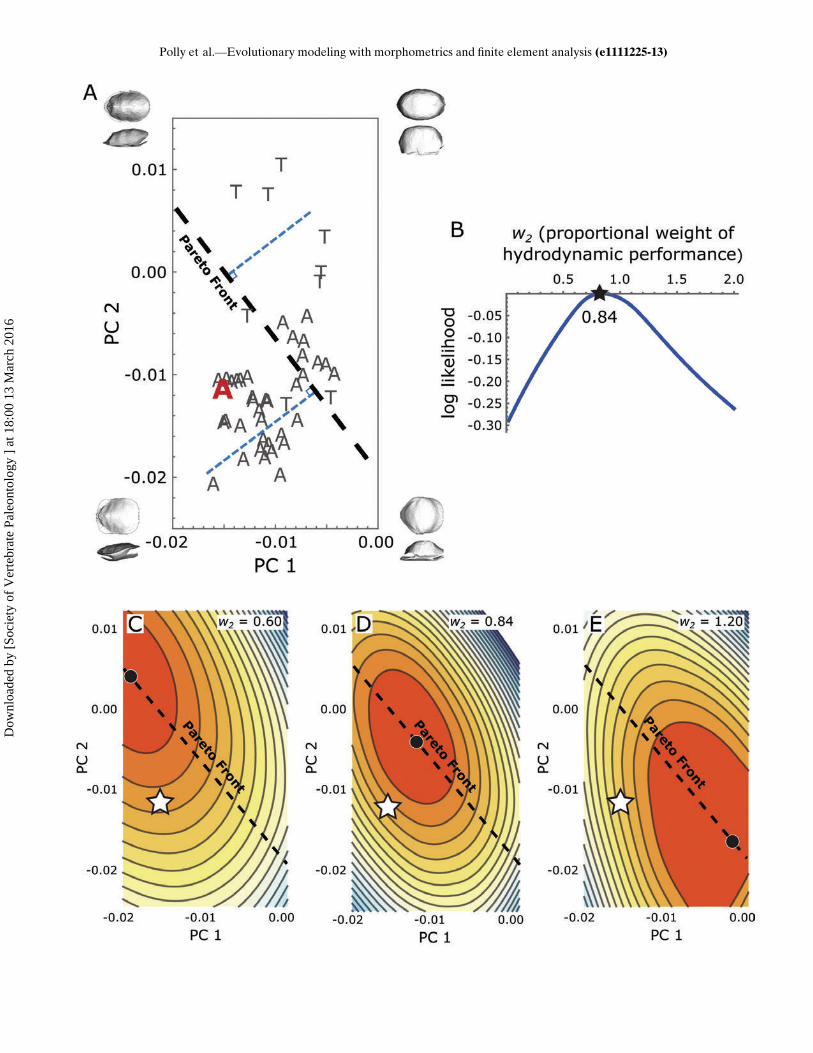
using the generalized linear model method of Martins and Han-sen (1997) with a Brownian motion model, which gives resultsidentical to those of the squared-change parsimony method ofMaddison (1991) and the one-rate maximum likelihood methodof Mooers and Schluter (1997). Phylogeny and original branchlengths are from Wiens et al. (2010), the same phylogeny usedby Stayton (2011). Branch lengths were transformed to timesince divergence using the method of Pagel (1992). The age ofthe base of the tree was set at 40 million years ago using the esti-mated age of the last common ancestor of crown Emydidae ascalibrated by Joyce et al. (2013) and Warnock et al. (2015),based on the oldest occurrence of Chrysemys antiqua in the Cha-dronian North American Land Mammal Age (NALMA) ofSouth Dakota (Hutchison, 1996; note that this calibration isyounger than that used by Lourenco et al., 2012).Our analyses were limited to the first two principal components

of shell morphospace, which account for 26% of the total vari-ance. Note that the morphometric analysis from which this mor-phospace was derived considered a larger clade than justemydids; readers interested in the details of the morphospace


Dow

nloa

ded

by [

Soci

ety

of V

erte

brat

e Pa

leon

tolo

gy ]

at 1

8:00

13

Mar

ch 2

016

construction and patterns of shape variation in the full clade arereferred to the original paper (Stayton, 2011). Ideally, our analy-ses could (and should) be carried out on the full multidimensionalmorphospace, but the analytical and conceptual complexityincreases enormously with three or more dimensions because theperformance surfaces become multidimensional manifolds thatare not easily illustrated or described (Arnold, 2003). Two dimen-sions serve better for demonstrating the principle, which is ourintention here. Our results should be interpreted with this limita-tion in mind. Customized permutation and Monte Carlo testswere used to assess statistical significance as needed (Manly,1991; Kowalewski and Novack-Gottshall, 2010). Each test isdescribed along with the corresponding results below.

Evolution of Functional Trade-offs in Emydidae

Here we apply the quantitative evolutionary frameworkdescribed above to test hypotheses about the role of functionalmorphology in the evolution of form that cannot be tested usingeither GM or FEA in isolation. Although we use the roles ofshell strength and hydrodynamic performance in the evolutionof shell shape in emydid turtles as an example, the followingquestions are of a form that can be generalized to almost anyclade.Can Shell Shape be Explained by the Two Functional

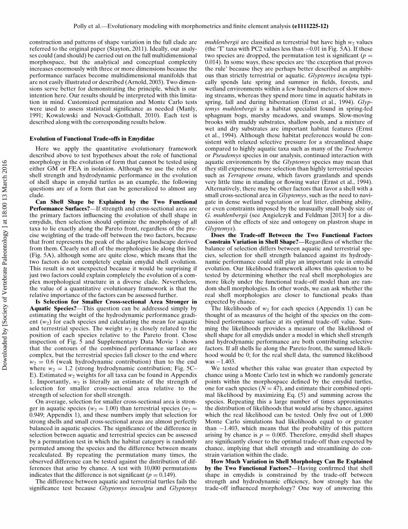
Performance Surfaces?—If strength and cross-sectional area arethe primary factors influencing the evolution of shell shape inemydids, then selection should optimize the morphology of alltaxa to lie exactly along the Pareto front, regardless of the pre-cise weighting of the trade-off between the two factors, becausethat front represents the peak of the adaptive landscape derivedfrom them. Clearly not all of the morphologies lie along this line(Fig. 5A), although some are quite close, which means that thetwo factors do not completely explain emydid shell evolution.This result is not unexpected because it would be surprising ifjust two factors could explain completely the evolution of a com-plex morphological structure in a diverse clade. Nevertheless,the value of a quantitative evolutionary framework is that therelative importance of the factors can be assessed further.Is Selection for Smaller Cross-sectional Area Stronger in

Aquatic Species?—This question can be addressed simply byestimating the weight of the hydrodynamic performance gradi-ent (w2) for each species and calculating the mean for aquaticand terrestrial species. The weight w2 is closely related to theposition of each species relative to the Pareto front. Closeinspection of Fig. 5 and Supplementary Data Movie 1 showsthat the contours of the combined performance surface arecomplex, but the terrestrial species fall closer to the end wherew2 D 0.6 (weak hydrodynamic contribution) than to the endwhere w2 D 1.2 (strong hydrodynamic contribution; Fig. 5C–E). Estimated w2 weights for all taxa can be found in Appendix1. Importantly, w2 is literally an estimate of the strength ofselection for smaller cross-sectional area relative to thestrength of selection for shell strength.On average, selection for smaller cross-sectional area is stron-

ger in aquatic species (w2 D 1.00) than terrestrial species (w2 D0.949; Appendix 1), and these numbers imply that selection forstrong shells and small cross-sectional areas are almost perfectlybalanced in aquatic species. The significance of the difference inselection between aquatic and terrestrial species can be assessedby a permutation test in which the habitat category is randomlypermuted among the species and the difference between meansrecalculated. By repeating the permutation many times, theobserved difference can be tested against the distribution of dif-ferences that arise by chance. A test with 10,000 permutationsindicates that the difference is not significant (p D 0.149).The difference between aquatic and terrestrial turtles fails the

significance test because Glyptemys insculpta and Glyptemys

muhlenbergii are classified as terrestrial but have high w2 values(the ‘T’ taxa with PC2 values less than ¡0.01 in Fig. 5A). If thesetwo species are dropped, the permutation test is significant (p D0.014). In some ways, these species are ‘the exception that provesthe rule’ because they are perhaps better described as amphibi-ous than strictly terrestrial or aquatic. Glyptemys inculpta typi-cally spends late spring and summer in fields, forests, andwetland environments within a few hundred meters of slow mov-ing streams, whereas they spend more time in aquatic habitats inspring, fall and during hibernation (Ernst et al., 1994). Glyp-temys muhlenbergii is a habitat specialist found in spring-fedsphagnum bogs, marshy meadows, and swamps. Slow-movingbrooks with muddy substrates, shallow pools, and a mixture ofwet and dry substrates are important habitat features (Ernstet al., 1994). Although these habitat preferences would be con-sistent with relaxed selective pressure for a streamlined shapecompared to highly aquatic taxa such as many of the Trachemysor Pseudemys species in our analysis, continued interaction withaquatic environments by the Glyptemys species may mean thatthey still experience more selection than highly terrestrial speciessuch as Terrapene ornata, which favors grasslands and spendsvery little time in standing or flowing water (Ernst et al., 1994).Alternatively, there may be other factors that favor a shell with asmall cross-sectional area inGlyptemys, such as the need to navi-gate in dense wetland vegetation or leaf litter, climbing ability,or even constraints imposed by the unusually small body size ofG. muhlenbergii (see Angielczyk and Feldman [2013] for a dis-cussion of the effects of size and ontogeny on plastron shape inGlyptemys).Does the Trade-off Between the Two Functional Factors

Constrain Variation in Shell Shape?—Regardless of whether thebalance of selection differs between aquatic and terrestrial spe-cies, selection for shell strength balanced against its hydrody-namic performance could still play an important role in emydidevolution. Our likelihood framework allows this question to betested by determining whether the real shell morphologies aremore likely under the functional trade-off model than are ran-dom shell morphologies. In other words, we can ask whether thereal shell morphologies are closer to functional peaks thanexpected by chance.The likelihoods of w2 for each species (Appendix 1) can be

thought of as measures of the height of the species on the com-bined performance surface at its optimal trade-off value. Sum-ming the likelihoods provides a measure of the likelihood ofshell shape for all emydids under a model in which shell strengthand hydrodynamic performance are both contributing selectivefactors. If all shells lie along the Pareto front, the summed likeli-hood would be 0; for the real shell data, the summed likelihoodwas ¡1.403.We tested whether this value was greater than expected by

chance using a Monte Carlo test in which we randomly generatepoints within the morphospace defined by the emydid turtles,one for each species (N D 47), and estimate their combined opti-mal likelihood by maximizing Eq. (5) and summing across thespecies. Repeating this a large number of times approximatesthe distribution of likelihoods that would arise by chance, againstwhich the real likelihood can be tested. Only five out of 1,000Monte Carlo simulations had likelihoods equal to or greaterthan ¡1.403, which means that the probability of this patternarising by chance is p D 0.005. Therefore, emydid shell shapesare significantly closer to the optimal trade-off than expected bychance, implying that shell strength and streamlining do con-strain variation within the clade.How Much Variation in Shell Morphology Can Be Explained

by the Two Functional Factors?—Having confirmed that shellshape in emydids is constrained by the trade-off betweenstrength and hydrodynamic efficiency, how strongly has thetrade-off influenced morphology? One way of answering this


Dow

nloa

ded

by [

Soci

ety

of V

erte

brat

e Pa

leon

tolo

gy ]

at 1

8:00

13

Mar

ch 2

016


Dow

nloa

ded

by [

Soci

ety

of V

erte

brat

e Pa

leon

tolo

gy ]

at 1

8:00

13

Mar

ch 2

016

question is to measure the proportion of variance in shell shapethat is correlated with the Pareto front (R2), which representsthe expected position of shells in morphospace if they were opti-mized by the two functional factors.The functional trade-off as measured by the Pareto front

explains 54.6% of the variance in shell shape (R2 D 0.564), whichis only marginally significant (p D 0.0662). R2 was estimated as 1¡ RSSPareto/SSTotal, where RSSPareto is the residual sum ofsquares around the Pareto front line and SSTotal is the total sumof squares of the PC1 and PC2 scores. Note that residual distan-ces are calculated orthogonal to the Pareto front, similar to anorthogonal or reduced major axis regression, because variationaround the line occurs along both the x and y axes. The p-valueswere derived from a Monte Carlo distribution of R2 for 10,000sets of random points in morphospace, each with N D 47. Thisresult suggests that an unknown factor or factors is systematicallycausing deviation of shell shape from the optimal trade-off valuebetween strength and cross-sectional area.Note, however, that because of the curvature of the combined

performance surfaces, points that are seemingly far from the cen-ter of the peak can still be near the top and thus in a favorableposition in terms of functional optimization (cf. SupplementaryData Movie 1). This nonlinearity between the location of thePareto front and the contours of the performance surface com-plicates interpretation of this particular result.What Factors Prevent Shell Shape from Being Optimized by

the Two Performance Factors?—The results so far show thatshell shape is optimized for a trade-off between strength andhydrodynamic efficiency more than expected by chance but thatthe variance explained by the trade-off is less than expected bychance. Furthermore, terrestrial and aquatic taxa do not differsignificantly in the extent to which they are optimized for hydro-dynamic performance (primarily because of the hydrodynamicshapes of the two terrestrialGlyptemys species). Possible explan-ations for the departure include genetic drift, phylogenetic iner-tia, the influence of genetic covariances, and the operation ofadditional unknown selective factors. We consider each of thesepossibilities in turn.In principle, drift is unlikely to explain the departure of shell

morphology from the strength–hydrodynamic trade-off becausethe variation away from the optimum is not random. Above weshowed that less variance was explained by the Pareto front thanexpected for random shell shapes because more variation in thedata set is orthogonal to the front than expected by chance. Driftis an example of a chance process and will produce a fairly circu-lar distribution of phenotypes (Fig. 3C).Note, however, that drift is more than fast enough to

explain some of the observed divergence among emydid shellshapes, though probably not all of it. The rate of drift pergeneration is a function of the genetic variance G and popu-lation size N (Eq. (1)). The genetic variance is the product ofthe phenotypic variance P and heritability h2. The amount ofphenotypic variance that will accumulate by drift alone in theabsence of selection can be estimated as h2Pt/N , where t is thetime in generations (Lande, 1976). We do not know the truevalues any of these parameters for emydids, but we can makereasonable estimates. The relevant population size parameterof interest is the average size of the breeding population ofeach entire species (not local population size) over the timespan that the group has been evolving. Local population sizesof Chrysemys picta often exceed 1,000 (Wilbur, 1975), and the

minimum viable population size of the species has been esti-mated at about 7,500 individuals (Reed et al., 2003). The cladehas been evolving for about 40 million years (Warnock et al.,2015) and generation length in C. picta is on average about10 years (Wilbur, 1975). If we start with these values andassume h2 to be about 0.5 (Cheverud, 1988), then a phenotypicvariance of about 2 £ 10¡7, or a total range of within-speciesvariation of about 0.001, is needed on each PC axis in order toaccount for the variation among species (Fig. 6A). Real within-species variation in shell shape is probably larger than this.Angielczyk et al.’s (2011) study of variation in emydid plastronshape found that within-species variation in several speciesmarginally overlapped with other species on the first two PCsof morphospace (e.g., Emys blandingii and Emys orbicularis).If carapace shape is proportionally as variable, then we can esti-mate a within-species range of variation of about 0.01 for eachspecies, which is equivalent to a phenotypic variance of about6 £ 10¡6. Our value of 7,500 individuals is likely a gross under-estimate of the breeding population for C. picta across its range,however. If heritability is higher at h2 D 0.75 and if populationsize is a more reasonable 100,000 breeding individuals per spe-cies, then drift could have produced a wider range of pheno-types than is observed (ca. 0.05 units on each PC axis; Fig. 6).The estimated rate of drift therefore suggests that selection is

acting to keep emydid shell shape closer to the Pareto front thanexpected from drift alone, similar to the scenario depicted inFig. 3C. In that scenario, selection gradients are relatively weakcompared to drift, allowing for substantial departure from theoptimum value while still keeping the distribution near the peak.Selection plus drift in nearly equal proportions would thereforebe enough to explain the observed shell shapes if it were not forthe observation that they are not distributed randomly withrespect to the Pareto front.Phylogenetic inertia is unlikely to explain the departure of

shell shape from the Pareto front. Phylogenetic inertia refers tothe inheritance of traits from an ancestor, implying that selectionhas not had the opportunity to transform the ancestral form toits current functional optimum. Given favorable conditions ofhigh heritability and small population size, drift alone canaccount for the occupation of all of the morphospace in our PCAplots without selection. This suggests that selection (which bydefinition is faster than drift) has had ample time to optimizespecies along the Pareto front if it was going to do so. Further-more, the Pareto front has not only been reached but crossedindependently at least 11 times by different branches (Fig. 6A).Finally, there is little phylogenetic structure to trade-off weight-ing (w2; Fig. 6B), contrary to what would be expected if selectionwere acting slowly enough that species had not had time to reachthe optimum. Common ancestry alone, therefore, does notexplain why some taxa lie away from the Pareto front.Within-species phenotypic and genetic covariances influence

the path of phenotypic evolution (Arnold et al., 2001) and cantherefore affect the distribution of species around the optimum.Such covariances can arise from developmental integration ormodularity, pleiotropy, or correlated selection. Within-speciescovariance structures are unknown for our taxa (they form partof the error term in Eq. (4)), but they are insufficient to explainthe failure of species to reach the optimum. Although thesecovariances would affect the path taken by the phenotype as itapproaches the selective peak (cf. Fig. 3A, Supplementary DataMovie 1), they do not prevent the phenotype from reaching the

FIGURE 5. Estimating trade-offs for real taxa using maximum likelihood. A, positions of aquatic (A) and terrestrial (T) species in morphospace.Chrysemys picta is highlighted in red (see Supplementary Data Fig. 1 for key to taxa). Two hypothetical selective factors are shown in blue at rightangles to the Pareto front; B, likelihood curve of the proportional weight of the cross-sectional area performance surface (w

2from Eq. (5)) for C. picta.

At the optimal value of w2 D 0.84, C. picta (star) is higher on the peak, D, than for other values of w

2(C, E). Black dots mark the peaks. Insets show

shell morphology at each corner of the morphospace.


Dow

nloa

ded

by [

Soci

ety

of V

erte

brat

e Pa

leon

tolo

gy ]

at 1

8:00

13

Mar

ch 2

016

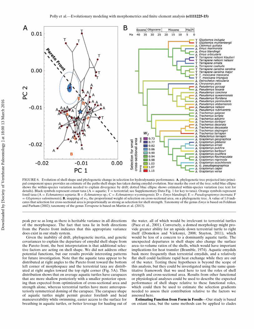
peak per se as long as there is heritable variance in all directionsof the morphospace. The fact that taxa lie in both directionsfrom the Pareto front indicates that this appropriate variancedoes exist in our study system.Given the inability of drift, phylogenetic inertia, and genetic

covariances to explain the departure of emydid shell shape fromthe Pareto front, the best interpretation is that additional selec-tive factors are acting on shell shape. We did not address otherpotential functions, but our results provide interesting patternsfor future investigation. Note that the aquatic taxa appear to bedistributed at right angles to the Pareto front toward the bottomleft corner of morphospace and the terrestrial taxa are distrib-uted at right angles toward the top right corner (Fig. 5A). Thisdistribution shows that on average aquatic turtles have carapacesthat are more shallow posteriorly with a smaller posterior open-ing than expected from optimization of cross-sectional area andstrength alone, whereas terrestrial turtles have more anteropos-teriorly symmetrical doming of the carapace. The carapace shapeof aquatic turtles might permit greater forelimb and headmaneuverability while swimming, easier access to the surface forbreathing in aquatic turtles, or better leverage for hauling out of

the water, all of which would be irrelevant to terrestrial turtles(Pace et al., 2001). Conversely, a domed morphology might pro-vide greater ability for an upside down terrestrial turtle to rightitself (Domokos and V�arkonyi, 2008; Stayton, 2011), whichwould be less of a concern to a dominantly aquatic turtle. Theunexpected departures in shell shape also change the surfacearea–to-volume ratios of the shells, which would have importantimplications for heat transfer (Bramble, 1974). Aquatic emydidsbask more frequently than terrestrial emydids, and a relativelyflat shell could facilitate rapid heat exchange while they are outof the water. Testing these hypotheses is beyond the scope ofthis analysis, but they could be investigated using the same quan-titative framework that we used here to test the roles of shellstrength and cross-sectional area. Results from other functionalor physiological analyses could be used to describe the expectedperformance of shell shape relative to these functional roles,which could then be used to estimate the selection gradientsneeded to assess their contribution relative to the factors weassessed here.Estimating Function from Form in Fossils—Our study is based

on extant taxa, but the same methods can be applied to clades

FIGURE 6. Evolution of shell shape and phylogenetic change in selection for hydrodynamic performance.A, phylogenetic tree projected into princi-pal component space provides an estimate of the paths shell shape has taken during emydid evolution. Star marks the root of the tree; solid blue ellipseshows the within-species variation needed to explain divergence by drift; dotted blue ellipse shows estimated within-species variation (see text fordetails). Black symbols represent extant taxa (A D aquatic; T D terrestrial; see Supplementary Data Fig. 1 for key to taxa). Orange symbols representfossil taxa (A D Echmatemys septaria; B D Echmatemys sp.; C D Echmatemys wyomingensis; D D Emys blandingii; E D Pseudograptemys inornata; FD Glyptemys valentinensis); B, mapping of w2, the proportional weight of selection on cross-sectional area, on a phylogenetic tree. A value of 1.0 indi-cates that selection for cross-sectional area is proportionally as strong as selection for shell strength. Taxonomy of the genus Emys is based on Feldmanand Parham (2002); taxonomy of the genus Terrapene is based on Martin et al. (2013).


Dow

nloa

ded

by [

Soci

ety

of V

erte

brat

e Pa

leon

tolo

gy ]

at 1

8:00

13

Mar

ch 2

016

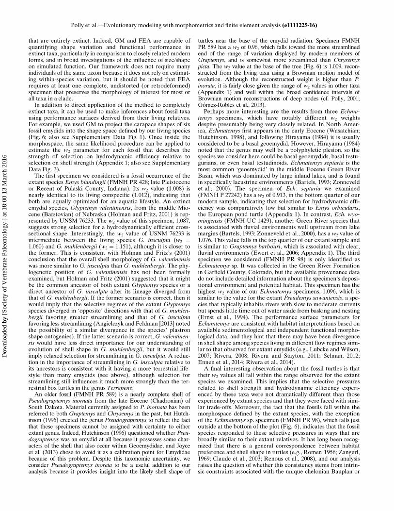
that are entirely extinct. Indeed, GM and FEA are capable ofquantifying shape variation and functional performance inextinct taxa, particularly in comparison to closely related modernforms, and in broad investigations of the influence of size/shapeon simulated function. Our framework does not require manyindividuals of the same taxon because it does not rely on estimat-ing within-species variation, but it should be noted that FEArequires at least one complete, undistorted (or retrodeformed)specimen that preserves the morphology of interest for most orall taxa in a clade.In addition to direct application of the method to completely

extinct taxa, it can be used to make inferences about fossil taxausing performance surfaces derived from their living relatives.For example, we used GM to project the carapace shapes of sixfossil emydids into the shape space defined by our living species(Fig. 6; also see Supplementary Data Fig. 1). Once inside themorphospace, the same likelihood procedure can be applied toestimate the w2 parameter for each fossil that describes thestrength of selection on hydrodynamic efficiency relative toselection on shell strength (Appendix 1; also see SupplementaryData Fig. 3).The first specimen we considered is a fossil occurrence of the

extant species Emys blandingii (FMNH PR 428; late Pleistoceneor Recent of Pulaski County, Indiana). Its w2 value (1.008) isnearly identical to its living conspecific (1.012), indicating thatboth are equally optimized for an aquatic lifestyle. An extinctemydid species, Glyptemys valentinensis, from the middle Mio-cene (Barstovian) of Nebraska (Holman and Fritz, 2001) is rep-resented by UNSM 76233. The w2 value of this specimen, 1.087,suggests strong selection for a hydrodynamically efficient cross-sectional shape. Interestingly, the w2 value of USNM 76233 isintermediate between the living species G. insculpta (w2 D1.060) and G. muhlenbergii (w2 D 1.151), although it is closer tothe former. This is consistent with Holman and Fritz’s (2001)conclusion that the overall shell morphology of G. valentinensiswas more similar to G. insculpta than G. muhlenbergii. The phy-logenetic position of G. valentinensis has not been formallyexamined, but Holman and Fritz (2001) suggested that it mightbe the common ancestor of both extant Glyptemys species or adirect ancestor of G. insculpta after its lineage diverged fromthat of G. muhlenbergii. If the former scenario is correct, then itwould imply that the selective regimes of the extant Glyptemysspecies diverged in ‘opposite’ directions with that of G. muhlen-bergii favoring greater streamlining and that of G. insculptafavoring less streamlining (Angielczyk and Feldman [2013] notedthe possibility of a similar divergence in the species’ plastronshape ontogenies). If the latter scenario is correct, G. valentinen-sis would have less direct importance for our understanding ofevolution of shell shape in G. muhlenbergii, but it would stillimply relaxed selection for streamlining in G. insculpta. A reduc-tion in the importance of streamlining in G. insculpta relative toits ancestors is consistent with it having a more terrestrial life-style than many emydids (see above), although selection forstreamlining still influences it much more strongly than the ter-restrial box turtles in the genus Terrapene.An older fossil (FMNH PR 589) is a nearly complete shell of

Pseudograptemys inornata from the late Eocene (Chadronian) ofSouth Dakota. Material currently assigned to P. inornata has beenreferred to both Graptemys and Chrysemys in the past, but Hutch-inson (1996) erected the genus Pseudograptemys to reflect the factthat these specimens cannot be assigned with certainty to eitherextant genus. Indeed, Hutchinson (1996) questioned whether Pseu-dograptemys was an emydid at all because it possesses some char-acters of the shell that also occur within Geoemydidae, and Joyceet al. (2013) chose to avoid it as a calibration point for Emydidaebecause of this problem. Despite this taxonomic uncertainty, weconsider Pseudograptemys inorata to be a useful addition to ouranalysis because it provides insight into the likely shell shape of

turtles near the base of the emydid radiation. Specimen FMNHPR 589 has a w2 of 0.96, which falls toward the more streamlinedend of the range of variation displayed by modern members ofGraptemys, and is somewhat more streamlined than Chrysemyspicta. The w2 value at the base of the tree (Fig. 6) is 1.009, recon-structed from the living taxa using a Brownian motion model ofevolution. Although the reconstructed weight is higher than P.inorata, it is fairly close given the range of w2 values in other taxa(Appendix 1) and well within the broad confidence intervals ofBrownian motion reconstructions of deep nodes (cf. Polly, 2001;G�omez-Robles et al., 2013).

Perhaps more interesting are the results from three Echma-temys specimens, which have notably different w2 weightsdespite presumably being very closely related. In North Amer-ica, Echmatemys first appears in the early Eocene (Wasatchian;Hutchinson, 1998), and following Hirayama (1984) it is usuallyconsidered to be a basal geoemydid. However, Hirayama (1984)noted that the genus may well be a polyphyletic plesion, so thespecies we consider here could be basal geoemydids, basal testu-gurians, or even basal testudinoids. Echmatemys septaria is themost common ‘geoemydid’ in the middle Eocene Green RiverBasin, which was dominated by large inland lakes, and is foundin specifically lacustrine environments (Bartels, 1993; Zonneveldet al., 2000). The specimen of Ech. septaria we examined(FMNH P 27242) has a w2 of 0.913, in the bottom quarter of ourmodern sample, indicating that selection for hydrodynamic effi-ciency was comparatively low but similar to Emys orbicularis,the European pond turtle (Appendix 1). In contrast, Ech. wyo-mingensis (FMNH UC 1429), another Green River species thatis associated with fluvial environments well upstream from lakemargins (Bartels, 1993; Zonneveld et al., 2000), has a w2 value of1.076. This value falls in the top quarter of our extant sample andis similar to Graptemys barbouri, which is associated with clear,fluvial environments (Ewert et al., 2006; Appendix 1). The thirdspecimen we considered (FMNH PR 98) is only identified asEchmatemys sp. It was collected in the Green River Formationin Garfield County, Colorado, but the available provenance datado not include detailed information about the specimen’s deposi-tional environment and potential habitat. This specimen has thehighest w2 value of our Echmatemys specimens, 1.096, which issimilar to the value for the extant Pseudemys suwaniensis, a spe-cies that typically inhabits rivers with slow to moderate currentsbut spends little time out of water aside from basking and nesting(Ernst et al., 1994). The performance surface parameters forEchamtemys are consistent with habitat interpretations based onavailable sedimentological and independent functional morpho-logical data, and they hint that there may have been divergencein shell shape among species living in different flow regimes simi-lar to that observed for extant emydids (e.g., Lubcke and Wilson,2007; Rivera, 2008; Rivera and Stayton, 2011; Selman, 2012;Ennen et al., 2014; Rivera et al., 2014).A final interesting observation about the fossil turtles is that

their w2 values all fall within the range observed for the extantspecies we examined. This implies that the selective pressuresrelated to shell strength and hydrodynamic efficiency experi-enced by these taxa were not dramatically different than thoseexperienced by extant species and that they were faced with simi-lar trade-offs. Moreover, the fact that the fossils fall within themorphospace defined by the extant species, with the exceptionof the Echmatemys sp. specimen (FMNH PR 98), which falls justoutside at the bottom of the plot (Fig. 6), indicates that the fossilspecies responded to these selective pressures in ways that arebroadly similar to their extant relatives. It has long been recog-nized that there is a general correspondence between habitatpreference and shell shape in turtles (e.g., Romer, 1956; Zangerl,1969; Claude et al., 2003; Renous et al., 2008), and our analysisraises the question of whether this consistency stems from intrin-sic constraints associated with the unique chelonian Bauplan or


Dow

nloa

ded

by [

Soci

ety

of V

erte

brat

e Pa

leon

tolo

gy ]

at 1

8:00

13

Mar

ch 2

016

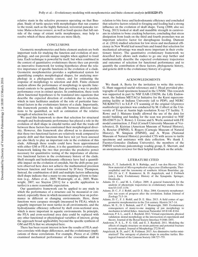
relative stasis in the selective pressures operating on that Bau-plan. Study of turtle species with morphologies that run counterto the trend, such as the highly flattened, terrestrial pancake tor-toiseMalacochersus tornieri, as well as fossil species that fall out-side of the range of extant turtle morphospace, may help toresolve which of these alternatives are more likely.

CONCLUSIONS

Geometric morphometrics and finite element analysis are bothimportant tools for studying the function and evolution of mor-phology, and can provide unique insights when applied to fossiltaxa. Each technique is powerful by itself, but when combined inthe context of quantitative evolutionary theory they can providean innovative framework for testing hypotheses about the rela-tive importance of specific functions in the evolution of a clade.Geometric morphometrics provides a sophisticated system forquantifying complex morphological shapes, for analyzing mor-phology in a phylogenetic context, and for estimating theresponse of morphology to selection and drift. Finite elementanalysis allows the performance of morphology in specific func-tional contexts to be quantified, thus providing a way to predictperformance even in extinct species. In combination, these toolsallow functional hypotheses to be translated into equations thatdescribe the expected direction of evolution due to selection,which in turn facilitates analysis of the role of particular func-tional factors in the evolutionary history of a clade. Importantly,this framework permits the trade-offs between different func-tions to be quantified, as well as estimation of the relativestrength of selection for each.We used this framework to show that selection for structural

strength and hydrodynamic performance has played a role in theevolution of shell shape in emydid turtles and that the trade-offbetween these factors has constrained their morphological diver-sity. However, this framework also allowed us to demonstratethat these two functional factors are relatively weak compared togenetic drift and that functions that have not yet been assessedare also likely to play an important role in the evolution of thisclade. Although these results could have been approximatedwith either GM or FEA alone, it is the quantitative evolutionaryframework linking the two that provides the predictive powernecessary for quantitative testing of the importance of alterna-tive functional factors in the evolutionary history of the clade.Shell strength and hydrodynamic efficiency have had a quantifi-able impact on the evolution of emydids, but the drift-prone pat-tern observed here does not achieve the mathematical precisionbetween function and form envisioned by D’Arcy Thompson.Instead, the combination of drift and multiple factors influencingshell shape indicate that a many-to-one mapping of form to func-tion (e.g., Alfaro et al., 2005; Wainwright, et al., 2005; Wain-wright, 2007; see Stayton [2011] for a specific application toturtles) is a more reasonable expectation.Our quantitative framework can be applied to any study in

which the performance of a structure can be measured or esti-mated, especially those in which measured values bear on perfor-mance in different or changing environments. Here, thosefunctions were carapace strength (measured by FEA), which isarguably important for most turtles in all environments, and thehydrodynamic efficiency reflected by shell cross-sectional area,which is more important in aquatic environments. In principle,the FEA and cross-sectional area data could be replaced withany other functional or physiological variables of interest, givingthe approach broad applicability beyond the specific synthesis ofGM and FEA that we attempted here.There has been recent interest in how the results of FEA anal-

yses correlate with shape differences, and the evolutionary impli-cations of those correlations. For example, Pierce et al. (2008)examined mechanical performance of the crocodilian skull in

relation to bite force and hydrodynamic efficiency and concludedthat selective factors related to foraging and feeding had a stronginfluence on the evolution of skull shape. Tseng (2008; also seeTseng, 2013) looked at skull and mandible strength in carnivor-ans in relation to bone cracking behaviors, concluding that stressdissipation from loads on the third and fourth premolars was animportant selective factor for durophagous feeding. Dumontet al. (2014) studied selection for low stress and mechanical effi-ciency in NewWorld leaf-nosed bats and found that selection formechanical advantage was much more important in their evolu-tionary history. The quantitative evolutionary framework wedescribed here allows such studies to go one step further andmathematically describe the expected evolutionary trajectoriesand outcomes of selection for functional performance and toquantify the contribution of these factors, phylogenetic history,and genetic drift to the evolutionary history of a group.

ACKNOWLEDGMENTS

We thank A. Berta for the invitation to write this review.G. Hunt suggested useful references and J. Head provided pho-tographs of fossil specimens housed in the UNSM. This researchwas supported in part by NSF EAR-1338298, the Lilly Endow-ment, the Indiana METACyt Initiative for the Karst supercom-puting facility at Indiana University (all to PDP), and NERCNE/K004751/1 to S.E.P. CT scanning of the original Glyptemysmuhlenbergii specimen was conducted by M. Colbert at the Uni-versity of Texas at Austin high resolution X-ray CT facility. T.Rowe and J. Maisano kindly allowed the use of the data formodel building and funding for the scan was provided to NSFIIS-028675 (to T. Rowe). I. Grosse and S. Werle assisted with FEmodel construction. J. Friel (Cornell University Museum of Ver-tebrates), D. Kizirian (American Museum of Natural History),A. Resetar (FMNH), S. Rogers (Carnegie Museum of NaturalHistory), W. Simpson (FMNH), and A. Wynn (NationalMuseum of Natural History) provided CTS with access to turtlespecimens and assistance with data collection. We thank J.Fuentes-Gonzalez (Indiana University), the members of theFMNH vertebrate paleontology reading group, E. Sherratt, andan anonymous reviewer for their helpful feedback on the article.

LITERATURE CITED

Abdala, F., T. Jashashvili, B. S. Rubidge, and J. van den Heever. 2014.New material of Microgomphodon oligocynus (Eutherapsida, Ther-ocephalia) and the taxonomy of southern African Bauriidae; pp.209–231 in C. F. Kammerer, K. D. Angielczyk, and J. Fr€obisch(eds.), Early Evolutionary History of the Synapsida. Springer,Dordrecht.

Adams, D. C., and M. L. Collyer. 2009. A general framework for theanalysis of phenotypic trajectories in evolutionary studies. Evolu-tion 63:1143–1154.

Adams, D. C., F. J. Rohlf, and D. E. Slice. 2004. Geometric morphomet-rics: ten years of progress after the revolution. Italian Journal ofZoology 71:5–16.

Adams, D. C., F. J. Rohlf, and D. E. Slice. 2013. A field comes of age:geometric morphometrics in the 21st century. Hystrix 24:7–14.

Alfaro, M. E., D. I. Bolnick, and P. C. Wainwright. 2005. Evolutionaryconsequences of many-to-one mapping of jaw morphology tomechanics in labrid fishes. American Naturalist 165:E140–E164.

Anderson, P. S. L., and E. J. Rayfield. 2012. Virtual experiments, physicalvalidation: dental morphology at the intersection of experiment andtheory. Journal of the Royal Society Interface 9:1846–1855.

Anderson, P. S. L., P. G. Gill, and E. J. Rayfield. 2011. Modeling theeffects of cingula structure on strain patterns and potential fracturein tooth enamel. Journal of Morphology 272:50–65.

Angielczyk, K. D., and C. R. Feldman. 2013. Are diminutive turtles mini-aturized? The ontogeny of plastron shape in emydine turtles. Bio-logical Journal of the Linnean Society 108:727–755.


Dow

nloa

ded

by [

Soci

ety

of V

erte

brat

e Pa

leon

tolo

gy ]

at 1

8:00

13

Mar

ch 2

016

Angielczyk, K. D., and H. D. Sheets. 2007. Investigation of simulated tec-tonic deformation in fossils using geometric morphometrics. Paleo-biology 33:125–148.

Angielczyk, K. D., C. R. Feldman, and G. R. Miller. 2011. Adaptive evo-lution of plastron shape in emydine turtles. Evolution 65:377–394.

Arbour, J. H., and C. M. Brown. 2014. Incomplete specimens in geometricmorphometric analyses.Methods inEcology andEvolution 5:16–26.

Arnold, S. J. 1983. Performance surfaces and adaptive landscapes. Amer-ican Zoologist 23:347–361.

Arnold, S. J. 2003. Performance surfaces and adaptive landscapes. Inte-grative and Comparative Biology 43:367–375.

Arnold, S. J., M. E. Pfrender, and A. G. Jones. 2001. The adaptive land-scape as a conceptual bridge between micro- and macroevolution.Genetica 112–113:9–32.

Bartels, W. S. 1993. Niche separation of fluvial and lacustrine reptilesfrom the Eocene Green River and Bridger Formations of Wyoming.Journal of Vertebrate Paleontology 13(3, Supplement):25A.

Benoit, J., T. Lehmann, M. Vatter, R. Lebrun, S. Merigeaud, L. Costeur,and R. Tabuce. 2015. Comparative anatomy and three-dimensionalgeometric morphometric study of the bony labyrinth of Bibymala-gasia (Mammalia, Afrotheria). Journal of Vertebrate Paleontology35:e930043, DOI:10.1080/02724634.2014.930043.

Berg, H. C. 1993. Random Walks in Biology. Princeton University Press,Princeton, New Jersey, 142 pp.

Bhullar, B.-A., Z. S. Morris, E. M. Sefton, A. Tok, M. Tokita, B. Nam-koong, J. Camacho, D. A. Burnham, and A. Abzhanov. 2015. Amolecular mechanism for the origin of a key evolutionary innova-tion, the bird beak and palate, revealed by an integrative approachto major transitions in vertebrate history. Evolution 69:1665–1677.

B€ohmer, C., O. W. M. Rauhut, and G. W€orheide. 2015. Correlationbetween Hox code and vertebral morphology in archosaurs. Pro-ceedings of the Royal Society B Biological Sciences 282:20150077.

Bookstein, F. L. 1987. Random walk and the existence of evolutionaryrates. Paleobiology 13:446–464.

Bookstein, F. L. 1989. Principal warps: thin-plate splines and the decom-position of deformations. IEEE Transactions on Pattern Analysisand Machine Intelligence 11:567–585.

Bookstein, F. L. 1991. Morphometric Tools for Landmark Data. Cam-bridge University Press, Cambridge, U.K., 435 pp.

Bookstein, F. L. 1996a. Biometrics, biomathematics and the morphomet-ric synthesis. Bulletin of Mathematical Biology 58:313–365.

Bookstein, F. L. 1996b. Standard formulae for the uniform shape compo-nent in landmark data; pp. 153–168 in L. F. Marcus, M. Corti, A.Loy, G. J. P. Naylor, and D. E. Slice (eds.), Advances in Morpho-metrics. Plenum Press, New York.

Bookstein, F. L. 1997. Landmark methods for forms without landmarks:localizing group differences in outline shape. Medical Image Analy-sis 1:225–243.

Bookstein, F. L. 1998. A hundred years of morphometrics. Acata Zoolog-ica Academiae Scientiarum Hungaricae 44:7–59.

Bookstein, F. L. 2013a. Allometry for the twenty-first century. BiologicalTheory 7:10–25.

Bookstein, F. L. 2013b. Random walks as a null model for high-dimen-sional morphometrics of fossil series: geometrical considerations.Paleobiology 39:52–74.

Bookstein, F. L. 2014. Measuring and Reasoning: Numerical Inference inthe Sciences. Cambridge University Press, Cambridge, U.K., 535 pp.

Bramble, D. M. 1974. Emydid shell kinesis: biomechanics and evolution.Copeia 1974:707–727.

Brassey, C. A., R. N. Holdaway, A. G. Packham, J. Ann�e, P. L.Manning, andW. I. Sellers. 2013.More than oneway of being aMoa: differences in legbone robustness map divergent evolutionary trajectories in Dinornithi-dae andEmeidae (Dinornithiformes). PLoSONE8(12):e82668.

Bright, J. A. 2014. A review of paleontological finite element models andtheir validity. Journal of Paleontology 88:760–769.

Bright, J. A., and E. J. Rayfield. 2011. Sensitivity and ex vivo validation offinite element models of the domestic pig cranium. Journal of Anat-omy 219:456–471.

Butler, M. A., and A. A. King. 2004. Phylogenetic comparative analysis: amodeling approach for adaptive evolution. American Naturalist164:683–695.

Button, D. J., E. J. Rayfield, and P. M. Barrett. 2014. Cranial biomechan-ics underpins high sauropod diversity in resource-poor environ-ments. Proceedings of the Royal Society B Biological Sciences281:1795. DOI: 10.1098/rspb.2014.2114.

Castanera, D., J. Colmenar, V. Sauqu�e, and J. I. Canudo. 2015. Geomet-ric morphometric analysis applied to theropod tracks from theLower Cretaceous (Berriasian) or Spain. Palaeontology 58:183–200.

Cheverud, J. M. 1982. Phenotypic, genetic, and environmental morpho-logical integration in the cranium. Evolution 36:499–516.

Cheverud, J. M. 1988. A comparison of genetic and phenotypic correla-tions. Evolution 42:958–968.

Claude, J. 2006. Convergence induced by plastral kinesis and phyloge-netic constraints in Testudinoidea: a geometric morphometricassessment. Fossil Turtle Research, Volume 1. Russian Journal ofHerpetology 13(Supplement):34–45.

Claude, J. 2008. Morphometrics in R. Springer, New York, 317 pp.Claude, J., E. Paradis, H. Tong, and J. C. Auffray. 2003. A geometric

morphometric assessment of the effects of environment and clado-genesis on the evolution of the turtle shell. Biological Journal of theLinnean Society 79:485–501.

Clough, R. W. 1990. Original formulation of the finite element method.Finite Elements in Analysis and Design 7:89–101.

Collyer, M. L., and D. C. Adams. 2013. Phenotypic trajectory analysis:comparison of shape change patters in evolution and ecology. Hys-trix 24:75–83.

Cox, P. G., M. J. Fagan, E. J. Rayfield, and N. Jeffery. 2011. Finite ele-ment modelling of squirrel, guinea pig and rat skulls: using geomet-ric morphometrics to assess sensitivity. Journal of Anatomy219:696–709.

Cullen, T. M., D. Fraser, N. Rybczynski, and C. Schr€oder�Adams. 2014.Early evolution of sexual dimorphism and polygyny in Pinnipedia.Evolution 68:1469–1484.

Curtis, N., M. E. H. Jones, S. E. Evans, P. O’Higgins, and M. J. Fagan.2013. Cranial sutures work collectively to distribute strain through-out the reptile skull. Journal of the Royal Society Interface 10:86.DOI:10.1098/rsif.2013.0442.

Curtis, N., M. E H. Jones, A. K. Lappin, S. E. Evans, P. O’Higgins,and M. J. Fagan. 2010. Comparison between in vivo and theo-retical bite performance: using multi-body modelling to predictmuscle and bite forces in a reptile skull. Journal of Biomechan-ics 43:2804–2809.

Dieleman, J., B. Van Bocxlear, C. Manntschke, D. W. Nyingi,D. Adriaens, and D. Verschuren. 2015. Tracing functional adapta-tion in African cichlid fishes through morphometric analysis of fossilteeth: exploring methods. Hydrobiologia 755:73–88.

Domokos, G., and P. V�arkonyi. 2008. Geometry and self-righting of tur-tle shells. Proceedings of the Royal Society B Biological Sciences275:11–17.

Drake, A. G., M. Coquerelle, and G. Colombeau. 2015. 3D Morphomet-ric analysis of fossil canid skulls contradicts the suggested domesti-cation of dogs during the late Paleolithic. Scientific Reports 5:8299.DOI:10.1038/srep08299.

Dryden, I. L., and K. V. Mardia. 1998. Statistics Shape Analysis. JohnWiley & Sons, Chichester, U.K., 376 pp.

Dumont, E. R., I. R. Grosse, and G. L. Slater. 2009. Requirements forcomparing the performance of finite element models of biologicalstructures. Journal of Theoretical Biology 256:96–103.

Dumont, E. R., J. Piccirillo, and I. R. Grosse. 2005. Finite-element analy-sis of biting behavior and bone stress in the facial skeletons of bats.Anatomical Record A 283A:319–330.

Dumont, E. R., J. L. Davis, I. R. Grosse, and A. M. Burrows. 2011. Finiteelement analysis of performance in the skulls of marmosets andtamarins. Journal of Anatomy 218:151–162.

Dumont, E. R., K. Samedevam, I. Grosse, O. M. Warsi, B. Baird, and L.M. Davalos. 2014. Selection for mechanical advantage underliesmultiple cranial optima in New World leaf-nosed bats. Evolution68:1436–1449.

Endler, J. A. 1986. Natural Selection in the Wild. Princeton UniversityPress, Princeton, New Jersey, 336 pp.

Ennen, J. R., M. E. Kalis, A. L. Patterson, B. R. Kreiser, J. E. Lovich, J.Godwin, and C. P. Qualls. 2014. Clinal variation or validation of asubspecies? A case study of the Graptemys nigrinoda complex(Testudines: Emydidae). Biological Journal of the Linnean Society111:810–822.

Ernst, C. H., J. E. Lovich, and R. W. Barbour. 1994. Turtles of the UnitedStates and Canada. Smithsonian Institution Press, Washington,D.C., 578 pp.

Ewert, M. A., P. C. H. Pritchard, and G. E. Wallace. 2006. Graptemysbarbouri, Barbour’s Map Turtle; pp. 260–272 in P. A. Meylan (ed.),


Dow

nloa

ded

by [

Soci

ety

of V

erte

brat

e Pa

leon

tolo

gy ]

at 1

8:00

13

Mar

ch 2

016

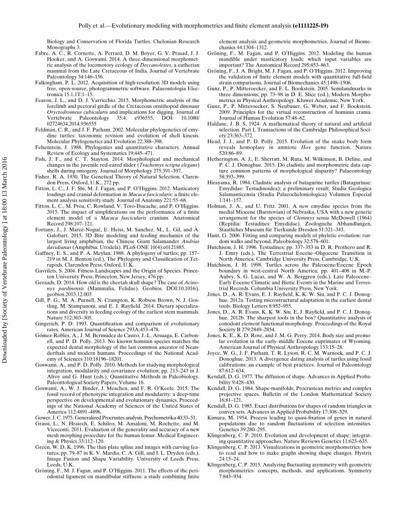
Biology and Conservation of Florida Turtles. Chelonian ResearchMonographs 3.

Fabre, A. C., R. Cornette, A. Perrard, D. M. Boyer, G. V. Prasad, J. J.Hooker, and A. Goswami. 2014. A three-dimensional morphomet-ric analysis of the locomotory ecology of Deccanolestes, a eutherianmammal from the Late Cretaceous of India. Journal of VertebratePaleontology 34:146–156.

Falkingham, P. L. 2012. Acquisition of high-resolution 3D models usingfree, open-source, photogrammetric software. Palaeontologia Elec-tronica 15.1.1T:1–15.

Fearon, J. L., and D. J. Varricchio. 2015. Morphometric analysis of theforelimb and pectoral girdle of the Cretaceous ornithopod dinosaurOryctodromeus cubicularis and implications for digging. Journal ofVertebrate Paleontology 35:4, e936555, DOI: 10.1080/02724634.2014.936555

Feldman, C. R., and J. F. Parham. 2002. Molecular phylogenetics of emy-dine turtles: taxonomic revision and evolution of shell kinesis.Molecular Phylogenetics and Evolution 22:388–398.

Felsenstein, J. 1988. Phylogenies and quantitative characters. AnnualReview of Ecology and Systematics 19:445–471.

Fish, J. F., and C. T. Stayton. 2014. Morphological and mechanicalchanges in the juvenile red-eared slider (Trachemys scripta elegans)shells during ontogeny. Journal of Morphology 275:391–397.

Fisher, R. A. 1930. The Genetical Theory of Natural Selection. Claren-don Press, Oxford, U.K., 272 pp.

Fitton, L. C., J. F. Shi, M. J. Fagan, and P. O’Higgins. 2012. Masticatoryloadings and cranial deformation inMacaca fascicularis: a finite ele-ment analysis sensitivity study. Journal of Anatomy 221:55–68.

Fitton, L. C., M. Proa, C. Rowland, V. Toro-Ibacache, and P. O’Higgins.2015. The impact of simplifications on the performance of a finiteelement model of a Macaca fascicularis cranium. AnatomicalRecord 298:107–121.

Fortuny, J., J. Marc�e-Nogu�e, E. Heiss, M. Sanchez, M., L. Gil, and �A.Galobart. 2015. 3D Bite modeling and feeding mechanics of thelargest living amphibian, the Chinese Giant Salamander Andriasdavidianus (Amphibia: Urodela). PLoS ONE 10(4):e0121885.

Gaffney, E. S., and P. A. Meylan. 1988. A phylogeny of turtles; pp. 157–219 in M. J. Benton (ed.), The Phylogeny and Classification of Tet-rapods. Clarendon Press, Oxford, U.K.

Gavrilets, S. 2004. Fitness Landscapes and the Origin of Species. Prince-ton University Press, Princeton, New Jersey, 476 pp.

Geraads, D. 2014. How old is the cheetah skull shape? The case ofAcino-nyx pardinensis (Mammalia, Felidae). Geobios. DOI:10.1016/j.geobios.2013.12.003

Gill, P. G., M. A. Purnell, N. Crumpton, K. Robson Brown, N. J. Gos-tling, M. Stampanoni, and E. J. Rayfield. 2014. Dietary specializa-tions and diversity in feeding ecology of the earliest stem mammals.Nature 512:303–305.

Gingerich, P. D. 1993. Quantification and comparison of evolutionaryrates. American Journal of Science 293A:453–478.

G�omez-Robles, A., J. M. Berm�udez de Castro, J.-L. Arsuaga, E. Carbon-ell, and P. D. Polly. 2013. No known hominin species matches theexpected dental morphology of the last common ancestor of Nean-derthals and modern humans. Proceedings of the National Acad-emy of Sciences 110:18196–18201.

Goswami, A., and P. D. Polly. 2010. Methods for studying morphologicalintegration, modularity and covariance evolution; pp. 213–243 in J.Alroy and G. Hunt (eds.), Quantitative Methods in Paleobiology.Paleontological Society Papers, Volume 16.

Goswami, A., W. J. Binder, J. Meachen, and F. R. O’Keefe. 2015. Thefossil record of phenotypic integration and modularity: a deep-timeperspective on developmental and evolutionary dynamics. Proceed-ings of the National Academy of Sciences of the United States ofAmerica 112:4891–4896.

Gower, J. C. 1975.Generalized Procrustes analysis. Psychometrika 40:33–51.Grassi, L., N. Hraiech, E. Schileo, M. Ansaloni, M. Rochette, and M.

Viceconti. 2011. Evaluation of the generality and accuracy of a newmesh morphing procedure for the human femur. Medical Engineer-ing & Physics 33:112–120.

Green, W. D. K. 1996. The thin-plate spline and images with curving fea-tures; pp. 79–87 in K. V. Mardia, C. A. Gill, and I. L. Dryden (eds.),Image Fusion and Shape Variability. University of Leeds Press,Leeds, U.K.

Gr€oning, F., M. J. Fagan, and P. O’Higgins. 2011. The effects of the peri-odontal ligament on mandibular stiffness: a study combining finite

element analysis and geometric morphometrics. Journal of Biome-chanics 44:1304–1312.

Gr€oning, F., M. Fagan, and P. O’Higgins. 2012. Modeling the humanmandible under masticatory loads: which input variables areimportant? The Anatomical Record 295:853–863.

Gr€oning, F., J. A. Bright, M. J. Fagan, and P. O’Higgins. 2012. Improvingthe validation of finite element models with quantitative full-fieldstrain comparisons. Journal of Biomechanics 45:1498–1506.

Gunz, P., P. Mitteroecker, and F. L. Bookstein. 2005. Semilandmarks inthree dimensions; pp. 73–98 in D. E. Slice (ed.), Modern Morpho-metrics in Physical Anthropology. Kluwer Academic, New York.

Gunz, P., P. Mitteroecker, S. Neubauer, G. Weber, and F. Bookstein.2009. Principles for the virtual reconstruction of hominin crania.Journal of Human Evolution 57:48–62.

Haldane, J. B. S. 1924. A mathematical theory of natural and artificialselection. Part I. Transactions of the Cambridge Philosophical Soci-ety 23:363–372.

Head, J. J., and P. D. Polly. 2015. Evolution of the snake body formreveals homoplasy in amniote Hox gene function. Nature520:86–89.

Hetherington, A. J., E. Sherratt, M. Ruta, M. Wilkinson, B. Deline, andP. C. J. Donoghue. 2015. Do cladistic and morphometric data cap-ture common patterns of morphological disparity? Palaeontology58:393–399.

Hirayama, R. 1984. Cladistic analysis of batagurine turtles (Batagurinae:Emydidae: Testudinoidea); a preliminary result. Studia GeologicaSalamanticensia (Studia Palaeocheloniologica) Volumen Especial1:141–157.

Holman, J. A., and U. Fritz. 2001. A new emydine species from themedial Miocene (Barstovian) of Nebraska, USA with a new genericarrangement for the species of Clemmys sensu McDowell (1964)(Reptilia: Testudines: Emydidae). Zoologische Abhandlungen,Staatliches Museum f€ur Tierkunde Dresden 51:321–343.

Hunt, G. 2006. Fitting and comparing models of phyletic evolution: ran-dom walks and beyond. Paleobiology 32:578–601.

Hutchison, J. H. 1996. Testudines; pp. 337–353 in D. R. Prothero and R.J. Emry (eds.), The Terrestrial Eocene–Oligocene Transition inNorth America. Cambridge University Press, Cambridge, U.K.

Hutchison, J. H. 1998. Turtles across the Paleocene/Eocene Epochboundary in west-central North America; pp. 401–408 in M.-P.Aubry, S. G. Lucas, and W. A. Berggren (eds.), Late Paleocene–Early Eocene Climatic and Biotic Events in the Marine and Terres-trial Records. Columbia University Press, New York.

Jones, D., A. R. Evans, E. J. Rayfield, K. K. W. Siu, and P. C. J. Donog-hue. 2012a. Testing microstructural adaptation in the earliest dentaltools. Biology Letters 8:952–955.

Jones, D., A. R. Evans, K. K. W. Siu, E. J. Rayfield, and P. C. J. Donog-hue. 2012b. The sharpest tools in the box? Quantitative analysis ofconodont element functional morphology. Proceedings of the RoyalSociety B 279:2849–2854.

Jones, K. E., K. D. Rose, and J. M. G. Perry. 2014. Body size and premo-lar evolution in the early–middle Eocene euprimates of Wyoming.American Journal of Physical Anthropology 153:15–28.

Joyce, W. G., J. F. Parham, T. R. Lyson, R. C. M. Warnock, and P. C. J.Donoghue. 2013. A divergence dating analysis of turtles using fossilcalibrations: an example of best practices. Journal of Paleontology87:612–634.

Kendall, D. G. 1977. The diffusion of shape. Advances in Applied Proba-bility 9:428–430.

Kendall, D. G. 1984. Shape-manifolds, Procrustean metrics and complexprojective spaces. Bulletin of the London Mathematical Society16:81–121.

Kendall, D. G. 1985. Exact distributions for shapes of random triangles inconvex sets. Advances in Applied Probability 17:308–329.

Kimura, M. 1954. Process leading to quasi-fixation of genes in naturalpopulations due to random fluctuations of selection intensities.Genetics 39:280–295.

Klingenberg, C. P. 2010. Evolution and development of shape: integrat-ing quantitative approaches. Nature Reviews Genetics 11:623–635.

Klingenberg, C. P. 2013. Visualizations in geometric morphometrics: howto read and how to make graphs showing shape changes. Hystrix24:15–24.

Klingenberg, C. P. 2015. Analyzing fluctuating asymmetry with geometricmorphometrics: concepts, methods, and applications. Symmetry7:843–934.


Dow

nloa

ded

by [

Soci

ety

of V

erte

brat

e Pa

leon

tolo

gy ]

at 1

8:00

13

Mar

ch 2

016

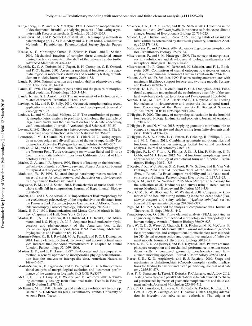
Klingenberg, C. P., and G. S. McIntyre. 1998. Geometric morphometricsof developmental instability: analyzing patterns of fluctuating asym-metry with Procrustes methods. Evolution 52:1363–1375.

Kowalewski, M., and P. Novack-Gottshall. 2010. Resampling methods inpaleontology; pp. 19–54 in J. Alroy and G. Hunt (eds.), QuantitativeMethods in Paleobiology. Paleontological Society Special Papers16.

Krauss, S., E. Monsongeo-Ornan, E. Zelzer, P. Fratzl, and R. Shahar.2009. Mechanical function of complex three-dimensional suturejoining the bony elements in the shell of the red-eared slider turtle.Advanced Materials 21:407–412.

Kupczik, K., C. A. Dobson, M. J. Fagan, R. H. Crompton, C. E. Oxnard,and P. O’Higgins. 2007. Assessing mechanical function of the zygo-matic region in macaques: validation and sensitivity testing of finiteelement models. Journal of Anatomy 210:41–53.

Lande, R. 1976. Natural selection and random drift in phenotypic evolu-tion. Evolution 30:314–334.

Lande, R. 1986. The dynamics of peak shifts and the pattern of morpho-logical evolution. Paleobiology 12:343–354.

Lande, R., and S. J. Arnold. 1983. The measurement of selection on cor-related characters. Evolution 37:1210–1226.

Lawing, A. M., and P. D. Polly. 2010. Geometric morphometrics: recentapplications to the study of evolution and development. Journal ofZoology 280:1–7.

Ledoux, L., and M. Boudadi-Maligne. 2015. The contribution of geomet-ric morphometric analysis to prehistoric ichnology: the example oflarge canid tracks and their implication for the debate concerningwolf domestication. Journal of Archaeological Science 61:25–35.

Levens, R. 1962. Theory of fitness in a heterogeneous environment. I. The fit-ness set and adaptive function.AmericanNaturalist 891:361–373.

Lourenco, J. M., J. Claude, N. Galtier, Y. Chiari. 2012. Dating crypto-diran nodes: origin and diversification of the turtle superfamily Tes-tudinoidea. Molecular Phylogenetics and Evolution 62:496–507.

Lubcke, G. M., and D. S. Wilson. 2007. Variation in shell morphology ofthe Western Pond Turtle (Actinemys marmorata Baird and Girard)from three aquatic habitats in northern California. Journal of Her-petology 41:107–114.

Macho, G. A., and I. R. Spears. 1999. Effects of loading on the biochemi-cal behavior of molars ofHomo, Pan, and Pongo. American Journalof Physical Anthropology 109:211–227.

Maddison, W. P. 1991. Squared-change parsimony reconstruction ofancestral states for continuous-valued characters on a phylogenetictree. Systematic Biology 40:304–314.

Magwene, P. M., and J. Socha. 2013. Biomechanics of turtle shell: howwhole shells fail in compression. Journal of Experimental Biology319:86–98.

Mallon, J. C., and J. S. Anderson. 2014. Implications of beak morphology forthe evolutionary paleoecology of the megaherbivorous dinosaurs fromthe Dinosaur Park Formation (upper Campanian) of Alberta, Canada.Palaeogeography, Palaeoclimatology, Palaeoecology 394:29–41.

Manly, B. F. J. 1991. Randomization and Monte Carlo Methods in Biol-ogy. Chapman and Hall, New York, 281 pp.

Martin, B. T., N. P. Bernstein, R. D. Birkhead, J. F. Koukl, S. M. Muss-mann, and J. S. Placyk, Jr. 2013. Sequence-based molecular phylo-genetics and phylogeography of the American box turtles(Terrapene spp.) with support from DNA barcoding. MolecularPhylogenetics and Evolution 68:119–134.

Mart�ınez-P�erez, C., E. J. Rayfield, M. A. Purnell, and P. C. J. Donoghue.2014. Finite element, occlusal, microwear and microstructural anal-yses indicate that conodont microstructure is adapted to dentalfunction. Palaeontology 57:1059–1066.

Martins, E. P., and T. F. Hansen. 1997. Phylogenies and the comparativemethod: a general approach to incorporating phylogenetic informa-tion into the analysis of interspecific data. American Naturalist149:646–667.

Mart�ın-Serra, A., B. Figueirido, and P. Palmqvist. 2014. A three-dimen-sional analysis of morphological evolution and locomotor perfor-mance of the carnivoran forelimb. PloS ONE 9:e85574.

McGill, B. J., B. J. Enquist, E. Weiher, and M. Westoby. 2006. Rebuild-ing community ecology from functional traits. Trends in Ecologyand Evolution 21:178–185.

McKinney, M. L. 1990. Classifying and analysing evolutionary trends; pp.28–58 in K. J. McNamara (ed.), Evolutionary Trends. University ofArizona Press, Tucson.

Meachen, J. A., F. R. O’Keefe, and R. W. Sadleir. 2014. Evolution in thesabre-tooth cat, Smilodon fatalis, in response to Pleistocene climatechange. Journal of Evolutionary Biology 27:714–723.

Meloro, C., A. Hudson, and L. Rook. 2015. Feeding habits of extant andfossil canids as determined by their skull geometry. Journal of Zool-ogy 295:178–188.

Mitteroecker, P., and P. Gunz. 2009. Advances in geometric morphomet-rics. Evolutionary Biology 36:235–247.

Mitteroecker, P., and S. M. Huttegger. 2009. The concept of morphospa-ces in evolutionary and developmental biology: mathematics andmetaphors. Biological Theory 4:54–67.

Mitteroecker, P., P. Gunz, M. Bernhard, K. Schaefer, and F. L. Book-stein. 2004. Comparison of cranial ontogenetic trajectories amonggreat apes and humans. Journal of Human Evolution 46:679–698.

Mooers, A. Ø., and D. Schulter. 1999. Reconstructing ancestor states withmaximum likelihood support for one- and two-rate models. System-atic Biology 48:623–633.

Murdock, D. J. E., E. J. Rayfield, and P. C. J. Donoghue. 2014. Func-tional adaptation underpinned the evolutionary assembly of the ear-liest vertebrate skeleton. Evolution and Development 16:354–361.

Neenan, J. M., M. Ruta, J. A. Clack, and E. J. Rayfield. 2014. Feedingbiomechanics in Acanthostega and across the fish-tetrapod transi-tion. Proceedings of the Royal Society B Biological Sciences281:20132689. DOI: 10.1098/rspb.2013.2689.

O’Higgins, P. 2000. The study of morphological variation in the hominidfossil record: biology, landmarks and geometry. Journal of Anatomy197:103–120.

O’Higgins, P., and N. Milne. 2013. Applying geometric morphometrics tocompare changes in size and shape arising from finite elements anal-yses. Hystrix 24:126–132.

O’Higgins, P., S. N. Cobb., L. C. Fitton, F. Gr€oning, R. Phillips, J. Liu,and M. J. Fagan. 2011. Combining geometric morphometrics andfunctional simulation: an emerging toolkit for virtual functionalanalyses. Journal of Anatomy 218:3–15.

O’Higgins, P., L. C. Fitton, R. Phillips, J. Shi, J. Liu, F. Gr€oning, S. N.Cobb, and M. J. Fagan. 2012. Virtual functional morphology: novelapproaches to the study of craniofacial form and function. Evolu-tionary Biology 39:521–535.

O’Keefe, F. R., W. J. Binder, S. R. Frost, R. W. Sadlier, and B. Van Val-kenburgh. 2014. Cranial morphometrics of the dire wolf, Canisdirus, at Rancho La Brea: temporal variability and its links to nutri-ent stress and climate. Palaeontologia Electronica 17.1.17A:1–23.

Olsen, A. M., and M. W. Westneat. 2015. StereoMorph: an R package forthe collection of 3D landmarks and curves using a stereo cameraset-up. Methods in Ecology and Evolution 6:351–356.

Pace, C. M., R. W. Blob, and M. W. Westneat. 2001. Comparative kine-matics of the forelimb during swimming in the red-eared slider (Tra-chemys scripta) and spiny softshell (Apalone spinifera) turtles.Journal of Experimental Biology 204:3261–3271.

Pagel, M. D. 1992. A method for analysis of comparative data. Journal ofTheoretical Biology 156:431–442.

Panagiotopoulou, O. 2009. Finite element analysis (FEA): applying anengineering method to functional morphology in anthropology andhuman biology. Annals of Human Biology 36:609–623.

Parr, W. C. H., S. Wroe, U. Chamoli, H. S. Richards, M. R. McCurry, P.D. Clausen, and C. McHenry. 2012. Toward integration of geomet-ric morphometrics and computational biomechanics: new methodsfor 3D virtual reconstruction and quantitative analysis of finite ele-ment models. Journal of Theoretical Biology 310:1–14.

Pierce, S. E., K. D. Angielczyk, and E. J. Rayfield. 2008. Patterns of mor-phospace occupation and mechanical performance in extant croco-dilian skulls: a combined geometric morphometric and finiteelement modeling approach. Journal of Morphology 269:840–864.

Pierce, S. E., K. D. Angielczyk, and E. J. Rayfield. 2009. Shape andmechanics in thalattosuchian (Crocodylomorpha) skulls: implica-tions for feeding behaviour and niche partitioning. Journal of Anat-omy 215:555–576.

Piras, P., G. Sansalone, L. Teresi, T. Kotsakis, P. Colangelo, andA. Loy. 2012.Testing convergent and parallel adaptations in talpids humeralmechani-cal performance by means of geometric morphometrics and finite ele-ment analysis. Journal ofMorphology 273:696–711.

Piras, P., G. Sansalone, L. Teresi, M. Moscato, A. Profico, R. Eng, T. C.Cox, A. Loy, P. Colangelo, and T. Kotsakis. 2015. Digging adapta-tion in insectivorous subterranean eutherians. The enigma of


Dow

nloa

ded

by [

Soci

ety

of V

erte

brat

e Pa

leon

tolo

gy ]

at 1

8:00

13

Mar

ch 2

016

Mesoscalops montanensis unveiled by geometric morphometricsand finite element analysis. Journal of Morphology 276:1157–1171.

Polly, P. D. 2001. Paleontology and the comparative method: ancestralnode reconstructions versus observed node values. American Natu-ralist 157:596–609.

Polly, P. D. 2004. On the simulation of the evolution of morphologicalshape: multivariate shape under selection and drift. PalaeontologiaElectronica 7.2.7A:1–28.

Porro, L. B., K. A. Metzger, J. Iriarte-Diaz, and C. F. Ross. 2013. In vivobone strain and finite element modeling of the mandible ofAlligatormississippiensis. Journal of Anatomy 223:195–227.

Raff, R. A. 1996. The Shape of Life: Genes, Development, and the Evo-lution of Animal Form. University of Chicago Press, Chicago, 520pp.

Raup, D. M. 1977. Stochastic models in evolutionary paleobiology; pp.59–78 in A. Hallam (ed.), Patterns of Evolution as Illustrated in theFossil Record. Elsevier Science, Amsterdam.

Rayfield, E. J. 2005. Aspects of comparative cranial mechanics in the the-ropod dinosaurs Coelophysis, Allosaurus and Tyrannosaurus. Zoo-logical Journal of the Linnean Society 144:309–316.

Rayfield, E. J. 2007. Finite element analysis and understanding the bio-mechanics and evolution of living and fossil organisms. AnnualReview of Earth and Planetary Sciences 35:541–576.

Rayfield, E. J. 2011. Strain in the ostrich mandible during simulated peck-ing and validation of specimen-specific finite element models. Jour-nal of Anatomy 218:47–58.

Rayfield, E. J., D. B. Norman, C. C. Horner, J. R. Horner, P. M. Smith, J.J. Thomason, and P. Upchurch. 2001. Cranial design and function ina large theropod dinosaur. Nature 409:1033–1037.

Reed,D.H., J. J.O’Grady,B.W.Brook, J.D.Ballou, andR.Frankham. 2003.Estimates of minimum viable population sizes for vertebrates and fac-tors influencing those estimates. Biological Conservation 113:23–34.

Rega, E. A., K. Noriega, S. S. Sumida, A. Huttenlocker, A. Lee, and B.Kennedy. 2012. Healed fractures in the neural spines of an associ-ated skeleton of Dimetrodon: implications for dorsal sail morphol-ogy and function. Fieldiana Life and Earth Sciences 5:104–111.

Renous, S., F. de Lapparent de Broin, M. Depecker, J. Davenport, andV. Bels. 2008. Evolution of locomotion in aquatic turtles; pp. 97–138 in J. Wyneken, M. H. Godfrey, and V. Bels (eds.), Biology ofTurtles. CRC Press, Boca Raton, Florida.

Rhee, H., M. F. Horstemeyer, Y. Hwang, H. Lim, H. El Kadiri, and W.Trim. 2009. A study on the structure and mechanical behavior ofthe Terrapene carolina carapace: a pathway to design bio-inspiredsynthetic composites. Materials Science and Engineering C29:2333–2339.

Richmond, B. G., B. W. Wright, I. Grosse, P. C. Dechow, C. F. Ross, M.A. Spencer, and D. S. Strait. 2005. Finite element analysis in func-tional morphology. Anatomical Record A 283:259–274.

Rivera, G. 2008. Ecomorphological variation in shell shape of the fresh-water turtle Pseudemys concinna inhabiting different aquatic flowregimes. Integrative and Comparative Biology 48:769–787.

Rivera, G., and C. T. Stayton. 2011. Finite element modeling of shellshape in the freshwater turtle Pseudemys concinna reveals a trade-off between mechanical strength and hydrodynamic efficiency.Journal of Morphology 272:1192–1203.

Rivera, G., and C. T. Stayton. 2013. Effects of asymmetry on the strengthof the chelonian shell: a comparison of three species. Journal ofMorphology 274:901–908.

Rivera, G., J. N. Davis, J. C. Godwin, and D. C. Adams. 2014. Repeat-ability of habitat-associated divergence in shell shape of turtles.Evolutionary Biology 41:29–37.

Rohlf, F. J. 1993. Relative warp analysis and an example of its applicationto mosquito wings; pp. 131–159 in L. F. Marcus, E. Bello, and AGarc�ıa-Valdecasas (eds.), Contributions to Morphometrics. Mono-grafias del Museo Nacional de Ciencias Naturales, Madrid.

Rohlf, F. J. 1995. Multivariate analysis of shape using partial-warp scores;pp. 154–158 in K. V. Mardia and C. A. Gill (eds.), Proceedings inCurrent Issues in Statistical Shape Analysis. Leeds University Press,Leeds, U.K.

Rohlf, F. J. 1999. Shape statistics: Procrustes superimpositions and tan-gent spaces. Journal of Classification 16:197–223.

Rohlf, F. J., and F. L. Bookstein. 2003. Computing the uniform compo-nent of shape variation. Systematic Biology 52:66–69.

Rohlf, F. J., and L. F. Marcus. 1993. A revolution in morphometrics.Trends in Ecology and Evolution 8:129–132.

Rohlf, F. J., and D. E. Slice. 1990. Extensions of the Procrustes methodfor the optimal superimposition of landmarks. Systematic Zoology39:40–59.

Romer, A. S. 1956. Osteology of the Reptiles. University of ChicagoPress, Chicago, 772 pp.

Ross, C. F., M. A. Berthaume, P. C. Dechow, J. Iriarte-Diaz, L. B. Porro,B. G. Richmond, M. Spencer, and D. S. Strait. 2011. In vivo bonestrain and finite-element modeling of the craniofacial haft in catar-rhine primates. Journal of Anatomy 218:112–141.

Sampson, P. D., F. L. Bookstein, H. Sheean, and E. L. Bolson. 1996.Eigenshape analysis of left ventricular outlines from contrast ventri-culograms; pp. 131–152 in L. F. Marcus, M. Corti, A. Loy, G. J. P.Naylor, and D. E. Slice (eds.), Advances in Morphometrics. NATOASI Series, Series A: Life Science, New York.

Sansalone, G., T. Kotsakis, and P. Piras. 2015. Talpa fossilis or Talpaeuropaea? Using geometric morphometrics and allometric trajecto-ries of humeral moles remains from Hungary to answer a taxonomicdebate. Palaeontologia Electronica 18.2.42A:1–17.

Schwarz-Wings, D., A. C. Meyer, E. Frey, H.-R. Manz-Steiner, and R.Schumacher. 2009. Mechanical implications of pneumatic neck ver-tebrae in sauropod dinosaurs. Proceedings of the Royal Society B277:11–17.

Selman, W. 2012. Intradrainage variation in population structure, shapemorphology, and sexual dimorphism in the Yellow-blotched Saw-back, Graptemys flavimaculata. Herpetological Conservation Biol-ogy 7:427–436.

Serrano-Fochs, S., S. De Esteban-Trivigno, J. Marc�e-Nogu�e, J. Fortuny,and R. A. Fari~na. 2015. Finite element analysis of the Cingulatajaw: an ecomorphological approach to armadillo’s diets. PLoS ONE10(4):e0120653.

Shi, J., N. Curtis, L. C. Fitton, P. O’Higgins, and M. J. Fagan. 2012.Developing a musculoskeletal model of the primate skull: predict-ing muscle activations, bite force, and joint reaction forces usingmultibody dynamics analysis and advanced optimisation methods.Journal of Theoretical Biology 310:21–30.

Shoval, O., H. Sheftel, G. Shinar, Y. Hart, O. Ramote, A. Mayo, E.Dekel, K. Kavanagh, and U. Alon. 2012. Evolutionary trade-offs,Pareto optimality, and the geometry of phenotypic space. Science336:1157–1160.

Sigal, I. A., M. R. Hardisty, and C. M. Whyne. 2008. Mesh-morphingalgorithms from specimen-specific finite element modeling. Journalof Biomechanics 41:1381–1389.

Simpson, G. G. 1944. Tempo and Mode in Evolution. Columbia Univer-sity Press, New York, 237 pp.

Simpson, G. G. 1953. The Major Features of Evolution. Columbia Uni-versity Press, New York, 434 pp.

Slater, G. J., L. J. Harmon, D. Wegmann, P. Joyce, L. J. Revell, and M. E.Alfaro. 2011. Fitting models of continuous trait evolution to incom-pletely sampled comparative data using approximate Bayesian com-putation. Evolution 66:752–762.

Slice, D. E. 2001. Landmark coordinates aligned by Procrustes analysisdo no lie in Kendall’s shape space. Systematic Biology 50:141–149.

Slice, D. E. 2005. Modern morphometrics; pp. 1–45 in D. E. Slice (ed.),Modern Morphometrics in Physical Anthropology. Kluwer Aca-demic, New York.

Slice, D. E. 2007. Geometric morphometrics. Annual Review of Anthro-pology 36:261–281.

Spears, I. R., and G. A. Macho. 1998. Biomechanical behavior of modernhuman molars: implications for interpreting the fossil record. Amer-ican Journal of Physical Anthropology 106:467–482.

Stayton, C. T. 2009. Application of thin-plate spline transformations tofinite element models or, how to turn a bog turtle into a spotted tur-tle and analyze both. Evolution 63:1348–1355.

Stayton, C. T. 2011. Biomechanics on the half shell: functional perfor-mance influences patterns of morphological variation in the emydidturtle carapace. Zoology 114:213–223.

Stephens, P. R., and J. J. Wiens. 2003. Ecological diversification and phy-logeny of emydid turtles. Biological Journal of the Linnean Society79:577–610.

Stephens, P. R., and J. J. Wiens. 2008. Testing for evolutionary trade-offsin a phylogenetic context: ecological diversification and evolution oflocomotor performance in emydid turtles. Journal of EvolutionaryBiology 21:77–87.

Strait, D. S., B. G. Richmond, M. A. Spencer, C. F. Ross, P. C. Dechow,and B. A. Wood. 2007. Masticatory biomechanics and its relevance


Dow

nloa

ded

by [

Soci

ety

of V

erte

brat

e Pa

leon

tolo

gy ]

at 1

8:00

13

Mar

ch 2

016

to early hominid phylogeny: an examination of palatal thicknessusing finite-element analysis. Journal of Human Evolution 52:585–599.

Strait, D. S., Q. Wang, P. C. Dechow, C. F. Ross, B. G. Richmond, M. A.Spencer, and B. A. Patel. 2005. Modeling elastic properties in finite-element analysis: how much precision is needed to produce an accu-rate model? The Anatomical Record 283A:275–287.

Straight, D. S., I. R. Grosse, P. C. Dechow, A. L. Smith, Q. Wang, G. W.Weber, S. Neubauer, D. E. Slice, J. Chalk, B. G. Richmond, P. W.Lucas, M. A. Spencer, C. Schrein, B. W. Wright, C. Byron, and C. F.Ross. 2010. The structural rigidity of the cranium of Australopithe-cus africanus: implications for diet, dietary adaptations, and theallometry of feeding biomechanics. Anatomical Record 293:583–593.

Svensson, E., and R. Calsbeek. 2012. The Adaptive Landscape in Evolu-tionary Biology. Oxford University Press, Oxford, U.K., 376 pp.

Tallman, M., N. Amenta, E. Delson, S. R. Frost, D. Ghosh, Z. S. Kluk-kert, A. Morrow, and G. J. Sawyer. 2014. Evaluation of a newmethod of fossil retrodeformation by algorithmic symmetrization:crania of papionins (Primates, Cercopithecidae) as a test case. PloSOne 9(7):e0100833.

Tanner, J. B., E. R. Dumont, S. T. Sakai, B. L. Lundrigan, and K. E.Holekamp. 2008. Of arcs and vaults: the biomechanics of bone-cracking in spotted hyaenas (Crocuta crocuta). Biological Journal ofthe Linnean Society 95:246–255.

Thomason, J. J. 1991. Cranial strength in relation to estimated biting forcesin somemammals. Canadian Journal of Zoology 69:2326–2333.

Thompson, D’A. W. 1917. On Growth and Form. Cambridge UniversityPress, Cambridge, U.K., 793 pp.

Tseng, Z. J. 2008. Bone-cracking capability in the skull of Dinocrocutagigantea (Carnivora, Mammalia) reveals biomechanical conver-gence between hyaenids and percrocutids. Journal of VertebratePaleontology 28(3, Supplement):153A.

Tseng, Z. J. 2009. Cranial function in a late Miocene Dinocrocutagigantean (Mammalia: Carnivora) revealed by comparative finiteelement analysis. Biological Journal of the Linnean Society96:51–67.

Tseng, Z. J. 2013. Testing adaptive hypotheses of convergence with func-tional landscapes: a case study of bone-cracking hypercarnivores.PloS ONE 8:e65305.

Tseng, Z. J., and J. J. Flynn. 2015. Are cranial biomechanical simulationdata linked to known diets in extant taxa? A method for applyingdiet–biomechanics linkage models to infer feeding capability ofextinct species. PLoS ONE 10(4):e0124020.

Tseng, Z. J., and X. Wang. 2010. Cranial morphology of fossil dogs andadaptation for durophagy in Borophagus and Epicyon (Carnivora,Mammalia). Journal of Morphology 271:1386–1398.

Turtle TaxonomyWorking Group [Van Dijk, P. P., J. B. Iverson, A. G. J.Rhodin, H. B. Shaffer, and R. Bour]. 2014. Turtles of the world, 7thedition: annotated checklist of taxonomy, synonymy, distribution,with maps, and conservation status. Chelonian Research Mono-graphs 5:329–479.

Vega, C., and C. T. Stayton. 2011. Dimorphism in shell shape andstrength in two species of emydid turtle. Herpetologica 67:397–405.

Wade, M. J., and S. Kalisz. 1990. The causes of natural selection. Evolu-tion 44:1947–1955.

Wainwright, P. C. 2007. Functional versus morphological diversity inmacroevolution. Annual Review of Ecology, Evolution, and Sys-tematics 39:381–401.

Wainwright, P. C., M. E. Alfaro, D. I. Bolnick, and C. D. Hulsey. 2005.Many-to-one mapping of form to function: a general principle inorganismal design? Integrative andComparative Biology 45:256–262.

Wang, Q., S. A. Wood., I. R. Grosse, C. F. Ross, U. Zapata, C. D. Byron,B. W. Wright, and D. S. Straight. 2012. The role of sutures in bio-mechanical dynamic simulation of a macaque cranial finite elementmodel: implications for the evolution of craniofacial form. The Ana-tomical Record 295:278–288.

Warnock, R. C. M., J. F. Parham, W. G. Joyce, T. R. Lyson, and P. C. J.Donoghue. 2015. Calibration uncertainty in molecular dating analy-ses: there is no substitute for the prior evaluation of time priors.Proceedings of the Royal Society B Biological Sciences282:20141013. DOI: 10.1098/rspb.2014.1013.

Weber, G. W., and F. L. Bookstein. 2011. Virtual Anthropology: AGuide to a New Interdisciplinary Field. Springer, Vienna, Austria,423 pp.

Weber, G. W., F. L. Bookstein, and D. S. Strait. 2011. Virtual anthropol-ogy meets biomechanics. Journal of Biomechanics 44:1429–1432.

Wiens, J. J., C. A. Kuczynski, and P. R. Stephens. 2010. Discordant mito-chondrial and nuclear gene phylogenies in emydid turtles: implica-tions for speciation and conservation. Biological Journal of theLinnean Society 99:445–461.

Wilbur, H. M. 1975. The evolutionary and mathematical demography ofthe turtle Chrysemys picta. Ecology 56:64–77.

Wiley, D. F., N. Amenta, D. A. Alcantara, D. Ghosh, Y. J. Kil, E. Del-son, W. Harcourt-Smith, F. J. Rohlf, K. St. John, and B. Hamann.2005. Evolutionary morphing; pp. 431–438 in Visualization, 2005.Papers presented at IEEE VIS 05, Minneapolis, MN. Institute ofElectrical and Electronics Engineers, New York, New York, U.S.A.

Witmer, L. M. 1995. The Extant Phylogenetic Bracket and the impor-tance of reconstructing soft tissues in fossils; pp. 19–33 in J. Thoma-son (ed.), Functional Morphology in Vertebrate Paleontology.Cambridge University Press, Cambridge, U.K.

Wolff, J. 1892. Das Gesetz der Transformation der Knochen. HirschwaldVerlag, Berlin, 152 pp.

Wright, S. 1932. The roles of mutation, interbreeding, crossbreeding, andselection in evolution. Proceedings of the 6th International Con-gress on Genetics 1:356–366.

Wright, S. 1968. Evolution and the Genetics of Populations, Volume 1:Genetic and Biometric Foundations. University of Chicago Press,Chicago, 469 pp.

Wroe, S. 2008. Cranial mechanics compared in extinct marsupial andextant African lions using a finite-element approach. Journal ofZoology 274:332–339.

Wroe, S., P. Clausen, C. McHenry, K. Moreno, and E. Cunningham.2007. Computer simulation of feeding behavior in the thylacine anddingo as a novel test for convergence and niche overlap. Proceed-ings of the Royal Society B Biological Sciences 274:2819–2828.

Young, M. T., M. A. Bell, and S. L. Brusatte. 2011. Craniofacial form andfunction in Metriorhynchidae (Crocodylomorpha: Thalattosuchia):modelling phenotypic evolution with maximum-likelihood methods.Biology Letters 7:913–916.

Zangerl, R. F. 1969. The turtle shell; pp. 311–339 in C. Gans, A. D. Bel-lairs, and T. S. Parsons (eds.), The Biology of the Reptilia, Volume1. Academic Press, London.

Zapata, U., K. Metzger, Q. Wang, R. M. Elsey, C. F. Ross, and P. C.Dechow. 2010. Material properties of mandibular cortical bone inthe American alligator,Alligator mississippiensis. Bone 46:860–867.

Zelditch, M. L., D. L. Swiderski, and H. D. Sheets. 2012. Geometric Mor-phometrics for Biologists: A Primer, second edition. AcademicPress, Amsterdam, 478 pp.

Zelditch, M. L., D. L. Swiderski, H. D. Sheets, and W. L. Fink. 2004.Geometric Morphometrics for Biologists: A Primer. Elsevier,Amsterdam, 443 pp.

Zienkiewicz, O. C., J. P. De S. R. Gago, and D. W. Kelly. 1983. The hier-archical concept in finite element analysis. Computers and Struc-tures 16:53–65.

Zonneveld, J.-P., G. F. Gunnell, and W. S. Bartels. 2000. Early Eocenefossil vertebrates from the southwestern Green River Basin, Lin-coln and Uinta Counties, Wyoming. Journal of Vertebrate Paleon-tology 20:369–386.

Submitted May 30, 2015; revisions received September 15, 2015;accepted October 16, 2015.Handling editor: Richard Butler.


Dow

nloa

ded

by [

Soci

ety

of V

erte

brat

e Pa

leon

tolo

gy ]

at 1

8:00

13

Mar

ch 2

016

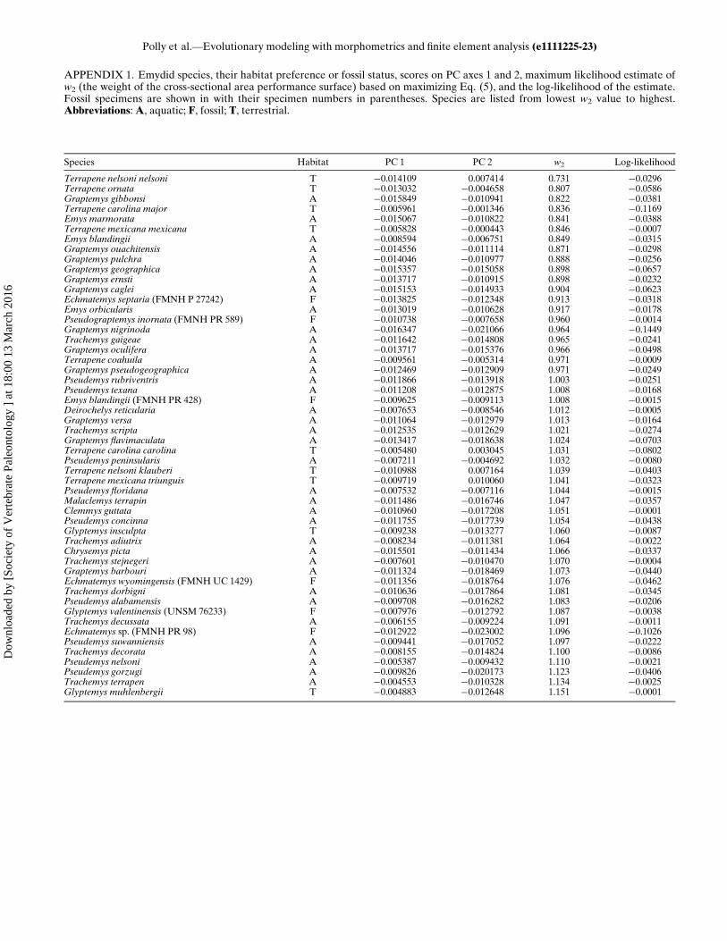
APPENDIX 1. Emydid species, their habitat preference or fossil status, scores on PC axes 1 and 2, maximum likelihood estimate ofw2 (the weight of the cross-sectional area performance surface) based on maximizing Eq. (5), and the log-likelihood of the estimate.Fossil specimens are shown in with their specimen numbers in parentheses. Species are listed from lowest w2 value to highest.Abbreviations:A, aquatic; F, fossil; T, terrestrial.

Species Habitat PC 1 PC 2 w2 Log-likelihood

Terrapene nelsoni nelsoni T ¡0.014109 0.007414 0.731 ¡0.0296Terrapene ornata T ¡0.013032 ¡0.004658 0.807 ¡0.0586Graptemys gibbonsi A ¡0.015849 ¡0.010941 0.822 ¡0.0381Terrapene carolina major T ¡0.005961 ¡0.001346 0.836 ¡0.1169Emys marmorata A ¡0.015067 ¡0.010822 0.841 ¡0.0388Terrapene mexicana mexicana T ¡0.005828 ¡0.000443 0.846 ¡0.0007Emys blandingii A ¡0.008594 ¡0.006751 0.849 ¡0.0315Graptemys ouachitensis A ¡0.014556 ¡0.011114 0.871 ¡0.0298Graptemys pulchra A ¡0.014046 ¡0.010977 0.888 ¡0.0256Graptemys geographica A ¡0.015357 ¡0.015058 0.898 ¡0.0657Graptemys ernsti A ¡0.013717 ¡0.010915 0.898 ¡0.0232Graptemys caglei A ¡0.015153 ¡0.014933 0.904 ¡0.0623Echmatemys septaria (FMNH P 27242) F ¡0.013825 ¡0.012348 0.913 ¡0.0318Emys orbicularis A ¡0.013019 ¡0.010628 0.917 ¡0.0178Pseudograptemys inornata (FMNH PR 589) F ¡0.010738 ¡0.007658 0.960 ¡0.0014Graptemys nigrinoda A ¡0.016347 ¡0.021066 0.964 ¡0.1449Trachemys gaigeae A ¡0.011642 ¡0.014808 0.965 ¡0.0241Graptemys oculifera A ¡0.013717 ¡0.015376 0.966 ¡0.0498Terrapene coahuila A ¡0.009561 ¡0.005314 0.971 ¡0.0009Graptemys pseudogeographica A ¡0.012469 ¡0.012909 0.971 ¡0.0249Pseudemys rubriventris A ¡0.011866 ¡0.013918 1.003 ¡0.0251Pseudemys texana A ¡0.011208 ¡0.012875 1.008 ¡0.0168Emys blandingii (FMNH PR 428) F ¡0.009625 ¡0.009113 1.008 ¡0.0015Deirochelys reticularia A ¡0.007653 ¡0.008546 1.012 ¡0.0005Graptemys versa A ¡0.011064 ¡0.012979 1.013 ¡0.0164Trachemys scripta A ¡0.012535 ¡0.012629 1.021 ¡0.0274Graptemys flavimaculata A ¡0.013417 ¡0.018638 1.024 ¡0.0703Terrapene carolina carolina T ¡0.005480 0.003045 1.031 ¡0.0802Pseudemys peninsularis A ¡0.007211 ¡0.004692 1.032 ¡0.0080Terrapene nelsoni klauberi T ¡0.010988 0.007164 1.039 ¡0.0403Terrapene mexicana triunguis T ¡0.009719 0.010060 1.041 ¡0.0323Pseudemys floridana A ¡0.007532 ¡0.007116 1.044 ¡0.0015Malaclemys terrapin A ¡0.011486 ¡0.016746 1.047 ¡0.0357Clemmys guttata A ¡0.010960 ¡0.017208 1.051 ¡0.0001Pseudemys concinna A ¡0.011755 ¡0.017739 1.054 ¡0.0438Glyptemys insculpta T ¡0.009238 ¡0.013277 1.060 ¡0.0087Trachemys adiutrix A ¡0.008234 ¡0.011381 1.064 ¡0.0022Chrysemys picta A ¡0.015501 ¡0.011434 1.066 ¡0.0337Trachemys stejnegeri A ¡0.007601 ¡0.010470 1.070 ¡0.0004Graptemys barbouri A ¡0.011324 ¡0.018469 1.073 ¡0.0440Echmatemys wyomingensis (FMNHUC 1429) F ¡0.011356 ¡0.018764 1.076 ¡0.0462Trachemys dorbigni A ¡0.010636 ¡0.017864 1.081 ¡0.0345Pseudemys alabamensis A ¡0.009708 ¡0.016282 1.083 ¡0.0206Glyptemys valentinensis (UNSM 76233) F ¡0.007976 ¡0.012792 1.087 ¡0.0038Trachemys decussata A ¡0.006155 ¡0.009224 1.091 ¡0.0011Echmatemys sp. (FMNH PR 98) F ¡0.012922 ¡0.023002 1.096 ¡0.1026Pseudemys suwanniensis A ¡0.009441 ¡0.017052 1.097 ¡0.0222Trachemys decorata A ¡0.008155 ¡0.014824 1.100 ¡0.0086Pseudemys nelsoni A ¡0.005387 ¡0.009432 1.110 ¡0.0021Pseudemys gorzugi A ¡0.009826 ¡0.020173 1.123 ¡0.0406Trachemys terrapen A ¡0.004553 ¡0.010328 1.134 ¡0.0025Glyptemys muhlenbergii T ¡0.004883 ¡0.012648 1.151 ¡0.0001


Dow

nloa

ded

by [

Soci

ety

of V

erte

brat

e Pa

leon

tolo

gy ]

at 1

8:00

13

Mar

ch 2

016

invited article combining geometric morphometrics and ...mypage.iu.edu/~pdpolly/papers/polly et al,...

Documents