G404 Geobiology Fall 2013

Name __________________________________

Lab 10 – Geometric morphometrics

Geometric morphometrics is a type of quantitative analysis of shape that is frequently used in paleontology. This technique allows shapes of structures such as bones to be represented as landmark points and analyzed. The main goals of geometric morphometrics are to study how specimens are similar or different in shape and to perform statistical analyses of shape.

In this lab you will learn to do a basic geometric morphometric analysis of Osteostracan head shields. The image data set comes from the following paper, which is one of the optional readings for yesterday’s lecture:

Sansom, R. S. 2009. Phylogeny, classification, and character polarity of the Osteostraci (Vertebrata). Journal of Systematic Paleontology, 7: 95-115.

In this lab you will collect the x,y coordinates of 13 landmarks from images of the head shields of 11 species of Osteostraci. You will import these into a geometric morphometric program called MorphoJ and create a “morphospace” plot to show similarities and differences among the fish and create a “shape model” that shows how individual Osteostracans differ from the rest.

Assignment: Perform the following steps. Turn in (1) a copy of the morphospace produced by your analysis (similar to Figure 4 below); (2) a series of five shape models (similar to Figure 5 below) representing the steps from 0.4 to -0.4 on Principal Component 2 of your morphospace (the vertical axis) (see Figure 6 below for example based on Principal Component 1).

A. Install ing programs

You should download and install the following programs, plugins, and data:

ImageJ – open-source software for image processing http://rsbweb.nih.gov/ij/download.html

Point Picker plugin for ImageJ http://bigwww.epfl.ch/thevenaz/pointpicker/

To install Point Picker follow these steps:

Mac OS X

1. Download the install image 2. Open the PointPicker.dmg 3. Copy the folder PointPicker to Applications -> ImageJ -> Plugins

Windows

1. Download the installation package

2

2. Unzip it 3. Copy the folder PointPicker to C:/Program Files/ImageJ/Plugins

Instructions for operating Point Picker are on the same page as the download files.

MorphoJ – Program package for geometric morphometrics from Chris Klingenberg http://www.flywings.org.uk/MorphoJ_page.htm

Image Fi les – Images of the head shields of Osteostraci from Sansom (2009). Unzip and place in a convenient place on your computer: Oncourse -> G404 -> Resources -> Misc -> Osteostraci Images for Lab 11

B. Collecting Landmark Coordinates

To collect landmark coordinates Using ImageJ, perform the following steps:

1. Place all your images in a single folder by themselves 2. Start ImageJ 3. open the first image

Repeat the following steps for each image

4. Start the PointPicker plugin: Plugins -> PointPicker -> PointPicker 5. Choose the pen tool (the one with a +) to add points 6. Carefully place each of your points on the image, always in the same order. If you

need to adjust the position, choose the move tool 7. When all points are placed, click the output button (the one with a piece of paper as

the icon). Use the Show option. 8. Highlight all the data, copy it, paste it into Excel with one blank line above, and one

blank line below 9. The x and y coordinates of your points are in the 2nd and 3rd columns. 10. Above the x-coordinates, enter the text "LM=" followed by the number of points (e.g.

LM=5) 11. Below the x-coordinates, enter the text "ID=" followed by the taxon name (e.g.

ID=Ateleaspis) 12. Clear the data window (by closing or clicking the red circle (MAC)) 13. Click the Return to ImageJ button (microscope icon) 14. Open next image 15. Repeat from Step 4 until all images are finished

3

Figure 1: screen shot from Excel showing what data look like at step 11 above.

C. Landmark Scheme for Osteostraci head shields

Use the following landmark scheme for your analysis. If you would like to modify it you may, but you must turn in a figure and description of the landmarks you used as an optional part of the assignment.

Figure 2: thirteen landmarks on the osteostracan head shield.

1. Anteriormost point on the midline of the head shield 2. Anteriormost point of olfactory pit 3. Pineal foramen (midline between eyes) 4. Posterior end of posterior field 5. Posteriormost point on the midline of the head shield 6. Posteriormost point on the left cornual plate 7. Posteriormost point of the left lateral field

1

2

3

4

5

6

7

811

910

12

13

4

8. Anteriormost point of the left lateral field 9. Center of left eye 10. Posteriormost point on the right cornual plate 11. Posteriormost point of the right lateral field 12. Anteriormost point of the right lateral field 13. Center of right eye

D. Reformatting landmark coordinates for MorphoJ

1. In Excel, highlight columns 2 & 3 from the first “LM=13” to the last “ID=Zenaspis_salweyi” and copy. For this lab that should be 165 rows with two columns.

2. In Word, use Paste Special to paste these rows as plain text. 3. Save the Word document as a plain text document somewhere convenient.

Figure 3: screen shot from Word showing what data look like in “TPS” form at step 2 above.

E. Getting Started in the MorphoJ program

1. Start MorphoJ and choose New Project from the file menu 2. Give the project a name on the first line and give your data set a name (e.g.,

Osteostraci landmarks. 3. Choose the TPS file type and choose the file you saved from Word in Step D

above.

F. Performing Geometric Morphometric Analysis in MorphoJ

1. Do Procrustes analysis to align the landmarks of your Osteostraci specimens. This step centers them on the same point, removes the differences in size, and

5

rotates the landmarks until they fit together. To do this, choose Preliminaries -> New Procrustes Fit Choose the option “Align by principal axes” Push the button “Perform Procrustes Fit” You will see a graphic showing the aligned specimens. The mean value of each landmark is numbered and the tiny dots scattered around are the landmarks of the individual Osteostracans.

2. Create a covariance matrix for your data. This is a necessary step for doing a Principal Components plot. To do this choose Preliminaries -> Generate Covariance Matrix Select Procrustes coordinates under data types Click the Execute button You won’t see any visible sign that anything happened

3. Perform a principal components analysis to show the similarities and differences between the Osteostracans in “morphospace”. To do this choose Variation -> Principal Components Anaysis Click the PC scores button on the graphics window that pops up Right click in the background and choose “Label Data Points” Points that cluster together have similar shapes, those that are far removed have different shapes.

Figure 4: morphospace plot should look something like this.

6

G. Visualizing shapes in morphospace with MorphoJ

Suppose you want to know what Boreaspis ceratops looks like relative to the others. Note that species is located at position -0.40 on principal component 1 (the main axis of the shape space).

To visualize this position in shape space, return to the PC shape changes frame Right click in background and “Change type of graph” to “Transformation Grid” Right click again and choose Change Scaling Factor and set to -0.40 (the position of Boreaspis) The lines show the difference between the landmarks in Boreaspsis (ends of the blue sticks) and the average Osteostracan shape (the numbered blue points). The grid is bent as though you had deformed the average Osteostracan shape into Boreaspsis. Note the right-click option called “Choose PC to Display”. You will need to change this to complete the assignment about modeling the shape differences along PC 2

This kind of plot is known as a “shape model”

Figure 5: Boreaspis shape model superimposed in Photoshop over the original image of Boreaspis ceratops to demonstrate how the lines and grid represent the transformation of an average Osteostracan into the shape of Boreaspsis ceratops.

7

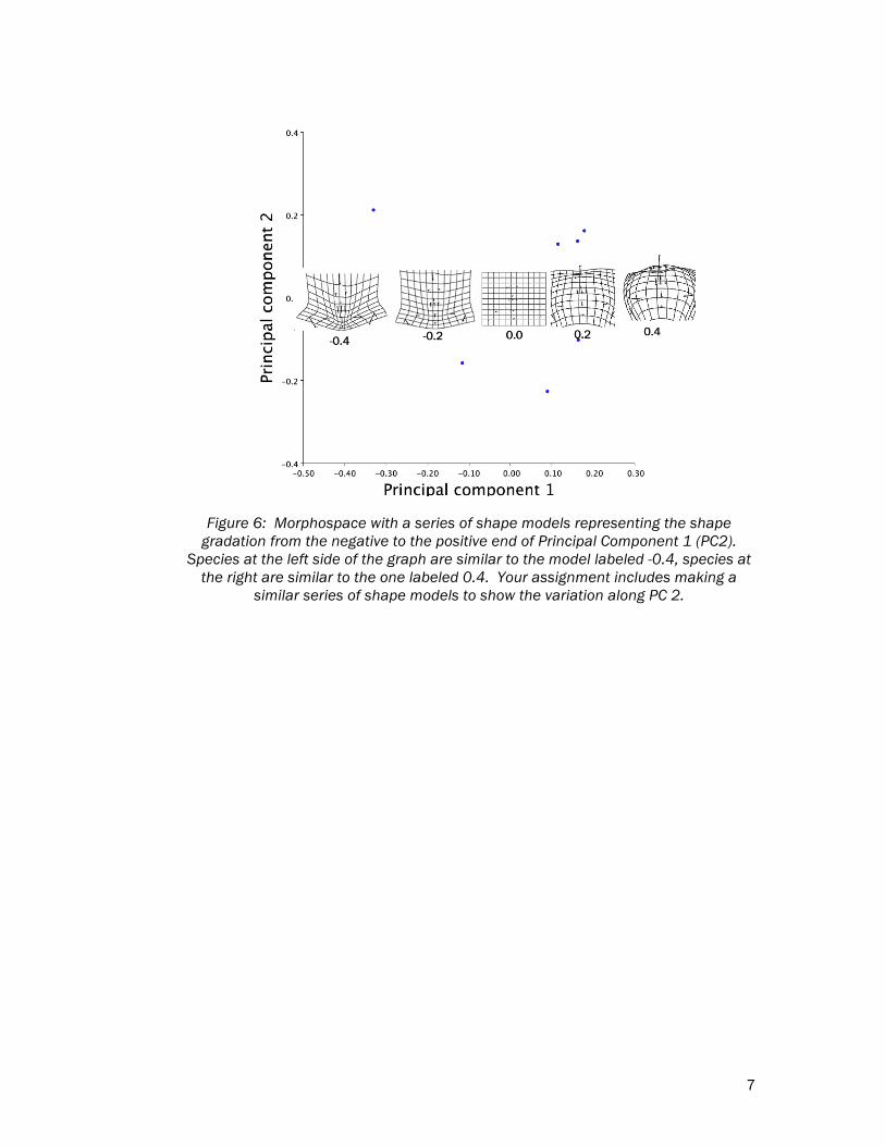
Figure 6: Morphospace with a series of shape models representing the shape gradation from the negative to the positive end of Principal Component 1 (PC2).

Species at the left side of the graph are similar to the model labeled -0.4, species at the right are similar to the one labeled 0.4. Your assignment includes making a

similar series of shape models to show the variation along PC 2.