io guide final - economicmodeling.com · emsi input-output guidebook, 2009 4. i. regional economics...

Input-OutputGuidebookEconomic Modeling Specialists Inc1187 Alturas DriveMoscow, ID 83843www.economicmodeling.com208.883.3500

contact information: Rob Sentz ([email protected])

A practical guide for regional economic impact analysisBy: M. Henry Robison, Founder and Senior Economist, EMSI

http://www.economicmodeling.com/

http://www.economicmodeling.com/

mailto:[email protected]

mailto:[email protected]

2 April, 2009

IntroductionOur nation’s economic woes have led to many ideas for the best way to transform our

economy and get it back on track. Many of these ideas are rooted in “Keynesian” eco-

nomic theory, which advocates for monetary and fiscal policy responses by the govern-

ment to stabilize and control the business cycle. The most significant instance of this is

the current American Recovery and Reinvestment Act1 (aka the “stimulus pack-

age”), which aims to spend unprecedented amounts of money on everything from infra-structure to health care to educational programs in order to create demand and spur

stagnant markets. There is much debate over the true effectiveness of this sort of inter-

vention, which is beyond the scope of this paper. For now we want to provide a practical

guide to make sure local planners know how to evaluate projects and programs based

on their importance to the region and especially on their potential return on investment.

Because of the sheer enormity and pervasive nature of the spending, the federal gov-

ernment would like to see a high level of accountability for organizations, institutions,

and programs that will be receiving this money.

A primary tool for this accountability and evaluating where spending might produce the greatest regional benefit is the input-output (IO) model. This tool is often misunderstood

and misused. However, if approached and applied correctly, IO can be a very powerful

and helpful tool for informing decisions—allowing planners to determine where dollars

will have their highest economic and workforce impacts.

In this paper we aim to provide an overview of IO for non-economists, provide some

useful illustrations and definitions, and serve as a basic orientation for local, state, fed-

eral planners so they can take advantage of this resource. While some of the material is

applicable to many economic models, we focus on the capabilities of EMSI’s Economic

Impact model.

If you have more questions about using IO modeling for your region, or would like

assistance, please feel free to contact us.

Hank Robison

EMSI Input-Output Guidebook, 2009 2

1 http://www.recovery.gov/

http://www.recovery.gov/

http://www.recovery.gov/

About the author

Dr. Henry Robison is a senior economist and co-principal of Economic Modeling Specialists Inc. (EMSI). He has over twenty years of experi-ence and a significant publications record in regional economic impact modeling and analysis. He is recognized for theoretical work blending regional input-output and spatial trade theory, and for development of community-level input-output modeling and analysis. He served 10 years as faculty member and consultant to the University of Idaho, where he secured a wide array of grants and contract research.

Dr. Robison's major EMSI consulting projects include design of the Utah Multiregional Input-Output (UMRIO) Model; work in partnership with Rutgers and Princeton University for the U.S. Department of Commerce Economic Development Administration (EDA) to assess the

effectiveness of EDA regional economic development grants; partner with New Jersey Institute of Technology and Rutgers University to develop the Federal Highway Administration's TELUS trans-portation project impact model; and extensive work with the U.S. Forest Service in ten western states on measuring the economic impacts of federal land management planning. He is also cur-rently working on a project to develop regional labor market analysis for the Middle East and North Africa.

A retrospective published in the journal of the Regional Science Association International listed Dr. Robison number eighteen on a list of the top one hundred "intellectual leaders of regional science" for the decade of the nineties (Papers in Regional Science, 83(1), 2004).


Table of Contents.....................................................................................................I. Regional Economics 101 5

.....................................................................................A. What is an input-output (IO) model? 6

.................................................................................................B. How are these models built? 7

............................................................................................................C. Why is IO Important? 8

...............................................................................................D. How are Multipliers Involved? 8

.............................................................................................II. Practical Applications of IO 10

.........................................................................................A. Descriptive and Predictive Uses 10

...................................................................B. Steps for Approaching IO Modeling & Analysis 10

...............................................................................................III. Understanding Multipliers 16

...................................................................................A. So where do multipliers come from? 17

.............................................................................................................B. Types of Multipliers 19

..........................................................................................C. Can multipliers get out of date? 21

................................................................D. Do multipliers depend on the size of the region? 21

..................................................................................IV. Avoiding Impact Modeling Pitfalls 22

............................................................A. Expressing impacts in terms of sales, not earnings 22

........................................................................B. Using total sales rather than trade margins 23

...................................................................................C. Failing to calculate true net impacts 23

............................................V. Using Input-Output for Economic Development Analysis 25

..................................................................................................A. Analyzing Economic Base 26

........................................................................B. Using IO to Conduct Industry Gap Analysis 30

........................................................................................VI. Defining Appropriate Regions 32

............................................................................................A. Functional Economic Regions 32

..........................................................................................................B. Central Place Theory 32

..........................................................................................................C. Complicating Factors 34

...............................................................................................................................Conclusion 36


I. Regional Economics 101This paper is for regional workforce and economic development professionals, education providers, regional policy makers, and others with an interest in regional workforce and economic development. Our first task is to introduce the study of regional economics in a way that is clear and relatively free of jargon.

We will begin with an illustration. Think of a drip falling into a bucket of water. When it hits the water it creates a splash. Very quickly the splash turns into ripples that radiate out, bounce, rebound, and eventually settle back to equilibrium. Overall, the bucket will gain or lose water depending on the rate of water dripping into it and the rate of water escaping through leaks.

Regional economies are a lot like this, in that money flows in and out of them, and the new flow creates “ripples” of economic growth. Households, businesses, and govern-ments are connected in a complex web of interdependent relationships based on produc-ing, selling, purchasing, and taxing goods and services, and each activity in one place tends to have effects on other places—just like the ripples caused by a drip falling into the bucket.

Regional economists seek to understand and, as much as possible, explain these interac-tions and how a change (especially an increase or decrease in jobs and earnings) in one area might affect other areas.

Let’s take an example at the national (not regional) level:1. A sharp decline in auto sales will quickly lead to a decline in auto dealerships and auto

manufacturing (e.g. less demand for cars = less production of cars). 2. A decline in auto manufacturing will lead to a decline in business by those that supply

goods and services to the manufacturers (e.g. parts suppliers). 3. If sales continue to fall, some car dealerships, parts suppliers, and possibly even manu-

facturers will go out of business, which means a loss of jobs and money they generate from their sales, purchases, and salaries.

4. With these jobs gone there will be less money circulating throughout the community and region.

5. The ultimate effect will be less money being spent on all kinds of goods and services: groceries, doctors, houses, and countless other services, which means that local indus-tries and services will eventually feel the effect of the downturn.


Each change in an economy produces additional ripples—sometimes large, sometimes small, that reverberate throughout the region and nation. If the ripples are small, many businesses will never actually notice them, or will be able to adjust to the fluctuations easily. However, if the ripples are large enough, many businesses could be capsized, which is where we find ourselves now.

Because we are talking about regions (not the entire nation) in this document, we’ll de-scribe modeling initial events and their effects only inside one region at a time. In other words, we have to define where the walls of the bucket are. This is where the bucket analogy breaks down a bit, because the reality is so much more complex. We might in-stead imagine the flow of money among businesses as a network of water tanks and pipes, and regional boundaries are like walls that the pipes may or may not pass through. Some stay inside the regional “room” and others go straight out through the wall, but the vast majority divide into many small pipes, some of which feed back into tanks (which represent businesses, government, and consumers) within the room, while the rest go out-side.

Regional economists have to decide where the walls are drawn, and then estimate and account for all the different flows in order to predict what the regional effect of a certain scenario will be—how much any new flow (or lack of flow) in one place will affect flows in other places, as well as the total amount of water (or wealth) in the room (region). A primary tool they use to do this is the regional input-output model.

A. What is an input-output (IO) model? An input-output model is a way of representing the flow of money in an economy, pri-marily among industries, while also accounting for government, households, and regional imports and exports. An industry is a group of business establishments that share similar end-products (or services) and processes for creating those products/services. Once the flow is represented in the model, a user can introduce events that change the flow (such as loss or gain of jobs/sales in one industry) and simulate its effects on each industry in the region, as well as the region as a whole.

This complex web of transactions can be arranged according to a particular accounting system called “input-output accounts.” They are called “input-output” because a portion of the output (i.e., sales) of one industry will appear as the input (i.e., purchases) of other industries. These accounts track the flow of money from one entity to the next, and from them we can get a sense of the interconnectedness of the industries, households, and government entities that occupy a given geographic space and build models to automati-


cally simulate and display these relationships. The input-output model therefore indi-cates how a change in one part of the economy will ultimately affect other parts based on these purchasing and selling relationships.

B. How are these models built? The main source of all IO models in the United States is the Industry Economic Ac-counts—especially the Annual and Benchmark Input-Output Accounts—produced by the Bureau of Economic Analysis (BEA), which in turn depends on data from other federal agencies. These tables provide a summary of how industries produce and consume com-modities at the national level, showing which industries produce and consume which commodities (including services), and how much. There are also some other rows and columns that account for money flows that are not strictly among industries, such as household consumption, government consumption, changes in inventories, exports and imports, compensation of employees, taxes, profits, and so on. In simple terms, these ta-bles are a form of accounting—like a business’s balance sheet. They show how various sales and expenses add up.

These tables are then manipulated, combined, and customized for smaller regions of the country using each region’s own industry mix and other information. This process is called “regionalizing” the model, and it is crucial because we need to estimate how much of each industry’s inputs are obtained locally (within the region), and how much of each industry’s outputs are exported outside the region. Without a good estimate of this, we have no idea what kind of feedback loops are occurring. To use our previous illustration, we wouldn’t know how many pipes are directing water flow back to tanks inside the room and how many are going out through the wall. If a local widget maker purchases all or most of its inputs from outside the region, then the region will not benefit as much when that company grows. But if there is a local supplier network, the benefits (and the downsides, too, if the company were to fail) will be amplified locally.

The ideal regionalization method, of course, would be to survey every business in the re-gion and ask about its suppliers and major clients, then classify and add up the responses by industry. But this is never feasible for many reasons, from cost to privacy concerns. So all the major models today depend heavily on non-survey techniques that use various re-gional data sources, including its industry mix, to estimate these values. Most models also allow some degree of additional customization if partial survey data are available.

The regionalization process results in a customized table for a region which shows what percentages of each industry’s “inputs” depend on the “outputs” from other industries. This table is the heart of any regional IO model.


C. Why is IO Important? Any sort of regional planning, spending, or investment requires stakeholders to

1. Express their goals clearly (i.e. create jobs, build new infrastructure, up-skill our workforce, attract new employers in industry A/B/C, etc.), and

2. Assess the effectiveness of alternative actions in achieving those goals.

Furthermore, common goals for development projects include:• increasing average earnings• increasing economic diversity• keeping more money in the local economy• expanding various industry clusters• increasing the overall quality of life• developing new industry or occupational areas.

These needs are always present for long-term regional development. But they are particu-larly important in our current economic situation, with so many job losses and so much money being spent on projects and programs meant to spur economic growth and help people find new employment.

In each case an IO model should be an essential part of the region’s toolkit, allowing stakeholders to discover areas where the economy might benefit most efficiently from new investment, and conversely, areas where additional attention is likely to be of less importance.

With development goals in place, IO is used to identify the best approach. For example, suppose there are several groups competing for various infrastructure improvements within a state. The IO model is used to simulate the potential impact of each decision (in terms of job, area industry impacts, and increased revenues). With the model you can be-gin to determine which project would have the best impact on the region—based on in-creased regional earnings, job creation, and how well the investment complements the current economic base. As a result, alternative uses of existing resources or investments, and the impact of declining or growing industries can be assessed in a data-driven, objec-tive way.

D. How are Multipliers Involved? You’ll sometimes hear the term “multiplier” used in discussions of economic policy and modeling, usually in the context of job creation. Basically, a multiplier represents how much some aspect of a model will change in response to changes coming from “outside” the model. Going back to our “pipes” analogy, suppose we have a model of the flow


among the water tanks and pipes in the room. The rate of flow from Tank A to Tank B in the room is a variable that’s entirely “inside” the model. But the model also depends on “outside” variables—in particular, how much total water is coming in. And if we change that amount permanently, we’ll change various rates of flow and water levels inside the room as well. We could then create multipliers to describe those effects in terms of the original change (final effect = the original change times the multiplier).

Economists use a lot of different multipliers to describe the effects of new private in-vestment, government spending, and even tax cuts. In this document, we’re interested in industry-by-industry sales, jobs, and earnings multipliers in the context of regional economies. We’ll discuss more details in Section III.


II. Practical Applications of IOA. Descriptive and Predictive UsesThe practical uses of input-output are of two kinds—descriptive and predictive.

In descriptive uses, the model simply informs users about the current regional economy:• Which industries have how many jobs and how much in earnings• What portion of an industry’s supply needs are likely purchased inside and outside

the region• Whether any industry clusters are present, and how well they are developed• What are the main sources of residents’ income• What is the composition of the region’s economic base (industries that tend to

bring money into the region rather than recycling money already there)

Using a model descriptively can reveal new knowledge about an area’s economy that would be impossible to get otherwise, or it may confirm anecdotal evidence. In either case, when correctly interpreted it provides a great starting point for community discus-sion.

Predictive uses are just as important, if not more so. The model can estimate the total impact of a hypothetical or actual looming event in one industry. The event and its impact are described in terms of changes in jobs, earnings, or sales. For example, entering into the model a loss of 100 jobs in a local industry might reveal a loss of 75 additional jobs based on multiplier effects in several other local industries. Without the model, planners would not have been as well prepared for these indirect effects on the local economy.

B. Steps for Approaching IO Modeling & AnalysisThe general steps involved in using a regional input-output model for policy analysis are:

Step 1: Define the region to be analyzedThe preparation and results of IO models depend greatly on how you choose to define the “region” to be analyzed. Do we analyze the “core” of a city, or should we include suburbs and bedroom communities too? In the case of “twin cities” do we isolate one, or treat them together as a single region? These issues are addressed in detail in Section VI, “De-fining Appropriate Regions.” The basic principle, however, is that you should not artifi-cially split up closely neighboring areas that have strong economic ties with each other—especially if there is a lot of commuting among them. Metropolitan Statistical Areas


(MSAs) are generally good boundaries for analyzing city economies, while smaller communities are often better defined using one or more ZIP codes.

Step 2a: Inform researchers and community stakeholders Regional input-output models convey a tremendous amount of baseline information right out of the box, before you’ve even started to run hypothetical scenarios (this is their “de-scriptive” function). As a result, it is always wise for policy makers to take stock of the current industry/occupation make-up of the region’s workforce, the relative magnitude of residents’ outside versus inside incomes, the importance of central functions (e.g., being a retail or transport hub), the leading industry clusters, and so on.

Some examples:• Your region has a big enough industry base to have $50 million in demand for en-

gineering services, but the local engineering services industry only has an output of $5 million. Using this as a basis for on-the-ground research, you could go on to discover which specific types of services are most needed, and then find out how your areas might attract more engineers.

• You discover that wineries are an emerging regional industry. However, the model shows that few or none of the key industries it is likely to purchase from—such as glass bottle manufacturers, fertilizer manufacturers, wholesalers, freight trucking, commercial printers, and cardboard packaging manufacturers—are located re-gionally. You decide it is feasible to recruit businesses in some of these categories into the area, and the result is that the region captures more of the wealth being generated by the wineries.

• You have anecdotal evidence that your town is becoming a “bedroom commu-nity” for a nearby city. But what is the economic effect of this? A look at the model shows that, on the positive side, outcommuters are earning an estimated $250 million, which they spend on services and retailers in your town. On the negative side, your town as a result has a disproportionate number of jobs in low-paying sectors like Services and Retail, bringing average earnings per job well below the state average. Your community then decides to create more good-paying job opportunities in the town itself, while also seeking to preserve the quality of life that has drawn commuters to live there.

This informational step can also generate good feedback from stakeholders with addi-tional local knowledge that can be used to customize the model (see next step).


Step 2b (Optional): Customize the model with local knowledgeRecall that most IO models are calibrated for a specific region with estimates for impor-tant variables such as the percentage of each industry’s requirements that come from in-region firms. This calibration is entirely mathematical and uses secondary (that is, non-survey) data sources, which may be incomplete. For detailed industry categories in smaller regions, even data such as the total jobs or earnings in some industries have been estimated in the model, since these numbers are often “suppressed” by government agen-cies to prevent their statistics from breaching the privacy of a particular business.

So, it is a good idea to spend some time with on-the-ground research (to whatever extent you can) in order to customize your model, especially if:

1. You are analyzing relatively small region (town or small city), especially a ZIP-code based region. The accuracy of any model’s estimates will decrease as the size of the region decreases.

2. Your region has a handful of important businesses that employ a significant por-tion of the area’s workforce (especially if your analysis involves the industries or related industries that these businesses are categorized under).

3. You intend to study the economic impact of a specific business’s expansion or contraction. IO models are intended to represent industries, or whole categories of similar businesses, not specific businesses. A particular business may have a sup-ply chain and production processes that differ from the average and that will af-fect the model’s results.

Some important variables to nail down with local knowledge and research include:1. Jobs and earnings by industry—you may need to refine exact figures for total

jobs and labor earnings in the region’s most important industries (and industries you specifically want to study), especially if there are only one or two big em-ployers in each of those industries.

2. Exports/imports—what percentage of each industry’s sales are to out-of-region vs. in-region customers? This also helps the model determine how much each in-dustry purchases from in-region vs. out-of-region suppliers. Industries that both (a) produce a lot of exports, and (b) purchase a lot of their requirements in the re-gion, will have greater multiplier effects and thus be more beneficial to the region.

3. Profits—the percentage of key industries’ profits that remain in the region (extent of local ownership). Locally-owned firms tend to keep all profits in the region, boosting their multiplier effect, while firms owned out-of-region will “leak” this income elsewhere.


Step 3: Translate policy issues/alternatives or looming events into direct effectsMost people want to use IO models not just for their descriptive features—they want to predict the effects of a looming event or policy alternative. To do this, we need to trans-late the situation facing us into a “direct effect,” which is a change caused by factors out-side the model, and which serves as the input to the model. The most common form of a direct effect is a positive or negative change in the jobs, sales, or earnings of one or more specific industries.

Here are some examples of specifying direct effects:• Translating policy issues to direct effects – It is not always immediately obvious

how a certain policy alternative can be translated into direct effects, but it is essen-tial that the modeler do it correctly. For instance, as the US government redefines building standards to make them more energy efficient and environmentally friendly, there will be a direct impact on industry—particularly construction, build-ing retrofitting, architecture, and building materials manufacturing. Policy makers can use IO models to simulate the impact of these projects at the local level and visualize how this could impact the region. In this case, local construction and retro-fitting companies would likely have more sales, and thus hire more workers.

• A construction/infrastructure project – A construction project will generate sales to the appropriate regional construction industry(ies), but it will also generate pur-chases of building materials like concrete, gravel, asphalt, steel, and so on. The re-searcher’s job is to delineate these dollar figures and find out how many will go to in-region vs. out-of-region industries. The result will be a set of direct effects that can all be entered into the model. However, it is also important to remember that jobs created by such projects, and predicted by the model, will only last as long as the project itself. More advanced and customized analysis is needed to figure out the more far-reaching effects of an infrastructure project. For example, a road im-provement project may allow more people to commute into the city center, which could cause residential construction growth in the suburbs and matching decline in the city center. Or a new fiber optic project may allow your town to attract a data center that will create 250 new jobs—but the model wouldn’t be able to predict those jobs simply based on the construction effort involved in laying the cables. Similarly, “quality-of-life” projects like a new park, aquarium, stadium, downtown revitalization, etc. are too complex to be judged with an IO model alone—it cannot predict, for instance, that more mobile young entrepreneurs and the jobs they create will move to your area (or stay there instead of moving elsewhere), just because of your downtown is now more attractive.


• Industry expansion or contraction – When your area is faced with the arrival/departure or contraction/expansion of a specific employer, the task of estimating direct effects is a lot easier. If a company announces that it will be laying off 100 workers or adding 100 workers, you can run this number through the model, in that company’s primary industry, to predict the direct and indirect impacts of a change in that industry on the region. Or if a prospective new employer wants $5 million in incentives from local governments, an IO model (with optional fiscal impact com-ponents) can help you determine the cost per job likely to be created, and the possi-ble return on investment of providing those incentives.

• An itemized purchases approach – If you have specific knowledge about an event or project, it may be more accurate to apportion out the total spending to multiple specific industries, rather than merely entering the lump sum as new sales in one industry. For example, if a textile factory is closing down, you could simply enter a loss of 100 jobs in the textile industry into the model. Or, you could manually ap-portion the value of the factory’s regional input purchases and workers’ earnings to the specific regional industries where they actually go—putting in a long list of smaller direct effects rather than one big one. This is especially useful if the fac-tory’s production processes and inputs are quite different from the national average. This approach is also often useful when evaluating construction projects.

Step 4: Enter direct effects into the modelNow let’s talk about how to run the analysis. First, we add in the estimated direct effects in terms of jobs, earnings, or sales gained or lost. There may be multiple changes in mul-tiple industries. The model runs millions of calculations in a few seconds and displays total impact of the chosen direct effect. The model also breaks down the change (positive or negative) in regional jobs and earnings by industry, and provides other information such as the different multipliers associated with the event.

ExampleLet’s look at an example that involves both construction and long-term job impacts. Sup-pose our area has a successful IT company that is considering moving some of its opera-tions outside the region. After some negotiation with local governments, the company decides to expand locally instead. The expansion will involve the construction of a new $20 million building, and is projected to save and create a total of 500 jobs in the region.

Construction Phase ImpactsSuppose the new building will take two years to complete, thus pumping $10 million a year for each of the two years into the regional construction sector. Using the IO model we first discover that the regional construction sector currently has about $225 million in


total sales. Running the model, we find that the addition of $10 million in sales in this sector should produce about 80 jobs in that sector, as well as about 65 additional jobs in other sectors. The jobs multiplier for commercial construction in our region is thus (80+65)/80 = 1.81. So for every one job from the initial change, another .81 jobs are cre-ated. The other industry areas most impacted by the addition of these jobs are local gov-ernment, restaurants, health care, and retail. There will also be an impact in construction materials manufacturing industries, like concrete products and fabricated metal products. The model also shows that the building phase will mean an influx of $6.3 million of earn-ings (labor income) into the area (note that earnings are very different from sales—not all of the original $10 million in sales will result in local earnings).

In-Place or Recurring ImpactsOnce the construction phase in our example is complete, these jobs and the resultant spending will most likely disappear, move elsewhere, or possibly be sustained by effects from other future projects. Remember—construction projects tend to have short-term im-pacts, unless there is solid evidence that they will create or save jobs in other industries that aren’t directly in the construction supply chain (e.g., new infrastructure needed to attract a major new employer to the area).

Next, let’s take a look at some of the potential long-term impacts of the event. In this case, we are creating/saving 500 jobs in a particular industry—e.g., “Computer facilities management services.” This needs no translation in order to become a “direct effect” we can enter into the model. When we do, we find that the addition of these jobs (with a jobs multiplier of about 1.57) will produce an additional 285 jobs throughout the region. The total annual impact of these new jobs could be $31 million worth of new earnings per year—much higher than the construction phase and also having the potential of staying in the economy for a much longer period of time.

Again, the IO model makes this a very straightforward exercise. The model will show the change, positive or negative, in regional jobs and earnings by industry (with detail down to the 6-digit NAICS code level if you are using EMSI’s EI model).


III. Understanding MultipliersIntroductionIn previous sections we have briefly introduced the concept of multipliers. Let’s take a minute to explain these and how they are very important to IO models. Although econo-mists talk about many kinds of multipliers, we are only concerned with regional multipli-ers in this guide.

For the purposes of regional IO, a multiplier is a number showing how changes (jobs, earnings, or sales) in one industry will propagate to other industries in a regional econ-omy. For example, a jobs multiplier of 3 means that a change of 100 jobs in that industry would lead to a total change of 300 jobs (3 x 100 = 300) in the whole economy. Note that this 300 includes the original 100 jobs, meaning the additional change is 200. In the study of IO, the original jobs are called the “direct” effect, while the additional jobs are called “indirect” effects.2

Let’s look at a real-life example to see how multipliers work in a region. Suppose a new company appears in a region, and begins making some product, the majority of which is exported outside the region. All these export sales result in “outside” money being brought into the region. This money enables the company to purchase local supplies and pay utilities, local taxes, local employee’s salaries, and so on, which means the total in-come in the region has increased, and local suppliers have more business which means they are likely to hire employees and spend more on their own inputs. As this new in-come passes from hand to hand, some is spent in the region and some “leaks out” at each stage. Adding up the amount spent inside the region at each stage of these transactions gives us the total effect of the original “outside income” of the new company. This effect can be expressed in either jobs or earnings. Suppose the new company’s payroll $2 mil-lion in earnings, but the total effect (including the original amount) is $2.8 million in earnings. The multiplier would then be 2.8 / 2 = 1.4.

Let’s take a simple example to illustrate the mechanics of multipliers. Suppose I’m part of the new company described above. For every $1,000 of total company sales, the com-pany uses the money in the following ways:


2 Strictly speaking, “indirect” effects involve the industries in the supply chain, while “induced” effects involve industry sales stimulated by added consumer spending. For convenience, in this guide we will refer to both kinds as simply “indirect” effects.

$500 Purchasing materials and supplies used to produce its goods$250 Payment of labor earnings in the form of salaries/wages, benefits, and other

compensation to employees$150 Taxes$100 Profits (also called “operating surplus”)

The earnings, taxes, and profits all represent the total value that the company has added to its inputs. This represents the wealth it has created and is also called value-added, out-put, or productivity.

Now let’s look at the “indirect” effects of these sales. Of the $500 spent on the company’s “inputs,” $200 is spent on in-region suppliers. Those suppliers then spend $50 on other local suppliers (as well as $50 on employee compensation, $25 on taxes, and $25 goes to profits), and these other suppliers do the same to their suppliers in an ongoing cycle, until the “leakage” of money from the region has reduced the original amount to zero.

Similarly, there are “induced” effects from the $250 in earnings that goes to the com-pany’s employees (we’ll assume they all live in the region). They spend these earnings on houses, food, utility bills, entertainment, and so on, with always a portion of the money staying in the region and a portion leaking out. These household-serving industries then spend a portion of this new income on their suppliers, employees, and so on, until “leak-age” again has reduced the amount remaining in the region to zero.

The multiplier comes from adding up the total amount remaining in the region during each cycle of spending, until it finally disappears through “leaks.” So, in one sense we do “re-count” the same money as it benefits each recipient in turn. But in addition, this money is creating new wealth at every step (just like planting a seed or making an in-vestment), since it allows each recipient to add more value by applying more labor to more materials. In the end, the original amount allows more goods to be produced and more services to be provided than otherwise, and the region as a whole is better off.

A. So where do multipliers come from? Regional multipliers arise naturally out of regional IO models, so we need to review the process of creating a regional IO model.

First, because of the lack of comprehensive local data, all regional models are created by “regionalizing” national values calculated by the Bureau of Economic Analysis. So mod-els primarily come from (a) the BEA’s national input-output accounts, and (b) regional purchase coefficients (RPCs).


Using the national input-output accounts we can create a table that quantifies, for each major industry, how much of the outputs from other industries is needed in order to pro-duce its own output. There are additional non-industry entities in this table too, like household consumption, profits, and taxes, which are used to complete the balance sheet. Every major model uses these national IO accounts in some way. Before applying it to a specific region, we have to generalize it by converting total national dollar amounts to percentages of total output, as well as account for the region’s actual industry mix. Then regional purchase coefficients (RPCs) are applied to each transaction to translate each industry’s “total inputs” to “only inputs purchased locally.”

RPCs represent the percentage of local demand that is satisfied by local supply. If your local construction industry has a $500 million total demand for ready-mix concrete, and it purchases $450 million of it locally, then that particular RPC would be 90%. If your local agriculture industry has a $500 million demand for tractors, but satisfies none of it from local manufacturers (which is quite common since there are relatively few places where tractors are manufactured), then that particular RPC would be 0%. High RPCs will result in higher multiplier effects since money spent on input requirements is being retained lo-cally. RPCs can be estimated in several ways by looking at each region’s industry mix (how much demand could possibly be supplied locally, and how much of that is actually likely to be supplied locally). While the details are beyond the scope of this document, suffice to say that EMSI uses a variation of the well-known Stevens technique3 for esti-mating RPCs, which has been widely discussed in the academic literature of regional IO for more than 20 years.

This whole accounting system tracks many links in the supply chain. As one dollar goes to one industry, portions of it are passed off to other local industries and another portion “leaks out” of the region completely. Then we look at all the other industries that got a piece of the original dollar and look at how much of those pieces go to other regional in-dustries or leak out. We continue this indefinitely until the portion of the original dollar still remaining in the region approaches zero. At each step, we sum up the amount that stayed in the region during that step. The grand total (plus the original dollar) is the final multiplier. In EMSI’s IO models, we use an earnings multiplier as our foundational mul-tiplier. This dollar-based earnings multiplier can also be converted to jobs or sales by us-ing the jobs-to-earnings and sales-to-earnings ratios in each industry.


3 Stevens, B.H., G.I. Treyz, D.J. Ehrlich, and J.R. Bower, 1983. “A New Technique for the Con-struction of Non-Survey Regional Input-Output Models,” International Regional Science Review, 8(3), 271-286.

B. Types of MultipliersThere are many types of multipliers depending on the model you use and what you are trying to measure. Following are the three main types of multipliers used in EMSI’s re-gional IO models.

1. Sales MultipliersSales multipliers show a change in total sales for one industry will change total sales in other industries. EMSI advises caution when using sales multipliers, since there is some double-counting involved. Instead, we prefer to express impacts in terms of jobs or earn-ings.

Here’s an example that illustrates the problem with sales multipliers. Suppose a consult-ing firm lands a $100,000 contract. Deciding that it could do the work more efficiently by using outside help, it does a portion of the work, keeps $20,000, and passes off $80,000 to another consultant to complete the rest of the work. This second consultant keeps $40,000 and passes off the other $40,000 to a third consultant, who completes the work alone. In terms of sales, we have this situation:

Consultant SalesFirst $100000Second $80000Third $40000Total $220000

This is misleading because we’re double-counting part of the sales at each step. However, in terms of earnings, the situation makes a lot more sense:

Consultant EarningsFirst $20000Second $40000Third $40000Total $100000

In this case, a sales multiplier would artificially inflate the impact, which is why we ad-vise caution when using sales multipliers and recommending using jobs or earnings mul-tipliers instead.


2. Jobs (Employment) MultipliersA jobs multiplier indicates how important an industry is in regional job creation. A jobs multiplier of 3, for example, would mean that for every new “direct” job in that industry, 2 more jobs would be created in other industries (for a total of 3 jobs). Typically, these additional jobs include many “fractions” of jobs spread over many industries.

Jobs multipliers are easily misinterpreted—jobs multipliers of 17 or higher are sometimes seen—but a high jobs multiplier for a set of one or more industries in an added-jobs sce-nario does not necessarily mean that attracting businesses in those industries to the region is the best or most viable option for regional economic growth.

Jobs multipliers are primarily tied to the type of industries in the scenario—indus-tries with a high capital/labor ratio typically have a high jobs multiplier, and vice versa. For example, a nuclear power plant might have only 20 workers, but “behind” each of those workers there are millions of dollars of equipment costs and millions of dollars of electricity being generated. Thus, if we bring 20 more nuclear power jobs into a region, that would involve a huge amount of investment flooding into the region (to build another nuclear power plant or increase the size of a current one) and millions of dollars in new sales and profits—which means more jobs.

Some of that money would go to the employees’ salaries, some would go to local con-struction companies, real estate, janitorial services, etc. The overall jobs multiplier would be impressive—each new job in nuclear power might support 14 other jobs scattered throughout the rest of the economy (i.e. a jobs multiplier of 15). However, the effort it takes to attract 20 jobs in nuclear power (with all the necessary infrastructure) is substan-tially more than to attract dozens more jobs in an industry with a lower jobs multiplier.

3. Earnings MultipliersIndustry earnings are the total amount of employee compensation paid out by employers in the industry. An earnings multiplier of 1.5 means that for every dollar of compensation entered as a “direct effect” in a new scenario, an additional $1.50 is paid out in wages, salaries, and other compensation throughout your economy. This is important for under-standing how a given scenario will effect not the number of jobs in your region, but the income-quality of those jobs. A scenario whose ripple effect brought two dozen lawyers and accountants into your region would have a much higher earnings multiplier than if that scenario brought the same number of indirect jobs mostly in food services and hotels.

Note that there is a tendency for industries with low earnings multipliers to have high jobs multipliers, and vice versa. In other words, it is a basic rule-of-thumb tradeoff that


industries tend to either create a lot of jobs with lower than average earnings, or fewer jobs with higher than average earnings.

C. Can multipliers get out of date?Yes, multipliers can get out of date, which is why you should use a regional IO model that uses the most recent data possible. Multipliers depend on the underlying IO model, which is always constructed using annual data for a single “base year.” Regional models in turn depend on the national input-output accounts and detailed information about a specific region’s industry mix, both of which change over time. The national accounts are released in detailed (“benchmark”) format every five years, along with a low-detail an-nual version. Regional data depend primarily on the BEA’s State and Local Personal In-come reports, the BLS’s Quarterly Census of Employment and Wages, and the Census Bureau’s County Business Patterns. These data sources have lots of industry and geo-graphic detail, but they also have a lag time of 6 months to 2 years. More current data sources (such as the Current Employment Survey) have a lag of only about 1 month, but have significantly less detail.

To produce our IO model, EMSI uses over 90 federal and state data sources and creates an integrated data set that balances accuracy with up-to-date relevance. We release new annual-average data on a quarterly schedule, constantly updating our model with new in-formation.

D. Do multipliers depend on the size of the region?Yes, multipliers are heavily influenced by region size because larger regions tend to sat-isfy more regional demand inside the region, simply because they are more economically diverse and transportation costs increase with region size. Small rural regions, on the other hand, tend to have low multipliers, because fewer goods and services can be pro-vided locally and so money “leaks out” much more quickly.

Because of this, it is very important to define regional boundaries in a way that is appro-priate to the analysis, and also never to use national or state-level multipliers for smaller regions. See part VI of this document, “Defining Appropriate Regions.”


IV. Avoiding Impact Modeling PitfallsIntroductionWhile the methods of conducting an IO analysis are straightforward, there are several common pitfalls that tend to overstate impacts, either because they fail to account for monies that leak outside of the region, or because they ignore monies that may be with-drawn or lost from the economy.

This is not meant to be a complete list, but three of the most common pitfalls in economic impact analysis are:

• Expressing impacts in terms of sales, not earnings• Using total sales rather than trade margins for retail and similar industries • Failing to calculate true net impacts

A. Expressing impacts in terms of sales, not earn-ings Sales comprise the total dollar amount collected in return for goods and services, while “earnings” refers to total wages, salaries, and other employment-related compensation. At the regional level, sales figures tend to be larger than income, thereby making impacts appear to be greater than they really are.

Consider the following example. Two visitors each spend $40,000 in a region. One visits a local auto dealer and purchases a new automobile. The other undergoes a medical pro-cedure at the local hospital. While both transactions amount to $40,000, they have widely different impacts on the local economy. Of the $40,000 spent for the automobile, perhaps $3,000 remain in the region as salesperson commissions and auto dealer income, while the other $37,000 leave the area for Detroit or Tokyo as wholesale payment for the new automobile. The hospital expenditure, on the other hand, retains perhaps $37,000 as wages for physicians, nurses, and assorted hospital employees (part of the region’s over-all income), while only $3,000 leave the area to pay for hospital supplies or help amortize building and equipment loans.

In terms of sales, both the automobile purchase and the medical procedure have the same impact. When expressed in terms of income, however, the former has a much smaller im-pact than the latter. As a true evaluation of regional impact, therefore, the use of earnings rather than sales is a far more accurate measure.


B. Using total sales rather than trade marginsThis pitfall is related to the previous one, because it deals with output in the retail, whole-sale, and related industries that primarily “re-sell” things they’ve purchased. When I buy a television from a local store, the store keeps a small percentage of the purchase price while the majority goes to pay the product’s wholesale and transportation costs. The TV is not a product of the store; rather, the store’s major “product” is actually a service—the service of selecting TVs, buying them in large quantities, transporting them, and display-ing them for purchase by consumers like me. So, we measure the total output of such in-dustries by their trade margins—or the difference between the cost of their products from the wholesaler and the cost to the consumer—not by their gross receipts. This is reflected in the model as well. In EMSI’s model, which shows estimated sales by industry, the “sales” shown are actually only the trade margin portion of sales.

So, when you are modeling purchases from these industries and want to enter the direct effect in terms of an increase in sales, you actually should enter the total increase in the trade margin. If automobile dealers have a 5% trade margin, for example, you would mul-tiply their gross sales increase or decrease by 5% to get the trade margin amount to enter into the model. Note: if you enter direct effects in terms of jobs or earnings, you do not run into this issue.

Finally, if in the rare case that any manufacturers of the type of product sold are also lo-cated in the region, you could allocate the remainder of the increase in sales (after trade margins are taken out) to the manufacturer’s industry.

C. Failing to calculate true net impactsWhile an economic event may generate direct regional impacts, failure to account for the money withdrawn from the economy as a result of that event results in overstatement of the impacts. As such, gross impacts must be adjusted to account for impacts that would have been generated had the event not taken place, and/or an alternative event had taken place.

Economists often explain this with the “Broken Window Fallacy.”4 When an errant baseball breaks a window pane on a house, the good news is that the local building sup-ply store benefits from the sale of a replacement window—a plus side for the economy. From one point of view, therefore, this visible transaction has not only contributed posi-tively and directly to economic growth, but also indirectly through a multiplier effect as


4 The name of the fallacy, and the whole explanation in this section, is summarized from Chapter 2 of Henry Hazlitt’s Economics in One Lesson (2nd edition; NY: Arlington House, 1979).

the supply store and its employees spend the added income from the sale of the replace-ment window. Given this reasoning, the careless batter could be naively regarded as a public benefactor, having created additional economic growth by breaking the window.

What’s missing is the invisible impact. The biggest loser is the owner of the broken win-dow and the biggest beneficiary is the building supply store. The store benefits but the homeowner loses because he now has less money to spend on other things. For example, the local clothing retailer loses because he didn’t receive an order for that new suit the homeowner had wanted but now can’t afford. Likewise, all the other vendors who would have benefited from the money earned and spent by the clothing retailer if the suit had been procured are also losers because the money was instead spent on replacing the bro-ken window. In the end, the errant baseball incident does not really add to economic growth at all. The clothing retailer and all of the vendors not benefiting from his business are the “invisible” losers. So at best, there’s no net effect; at worst, economic growth is actually hindered because the invisible loss could be greater than the visible gain.

The broken window fallacy illustrates the difference between gross and net impacts. Measuring only the gross—the transaction between the homeowner and the building sup-ply store—is only half the story. The other half is the adjustment needed to account for the money withdrawn from the economy to make that transaction, money that could have been spent elsewhere had the window not been broken. For the homeowner, that money is what he would have spent at the clothing retailer’s for a new suit, and the subsequent ripple effect that would have occurred as the clothing retailer spent the money earned. These effects should be subtracted from the effect created by the broken window to de-termine its net impacts.

So, make sure that the regional project you are evaluating is not a giant broken window. Always ask, what are the alternatives to this scenario, and what would their impacts be? An IO model alone cannot tell you this. It requires additional insight and knowledge of the local region and the specific project(s) involved.

And of course, pure dollar-value economic impact is not the only way to evaluate a pro-ject, especially public works projects. For example, a public park may have a negative impact because it costs money to maintain and supports only one or two jobs. However, citizens expect government to fund such projects to maintain quality of life in their com-munities, since the private sector would not undertake them given the conditions put on them by the public (e.g., free use of the park). And quality of life has indirect economic consequences as well—even if those consequences cannot be captured in an IO model.


V. Using Input-Output for Economic Development AnalysisIntroductionInput-output has not been used to its maximum potential in economic development. Often it is merely a political tool that helps to justify incentives for recruiting and retaining spe-cific companies in a region. By running impact scenarios and estimating multipliers, an IO model will tell you approximately how much one employer is “worth” to the regional economy.

But IO has far more potential to help economic development efforts, because of its ability to capture and analyze the structure of a regional economy, which is invaluable for meas-uring the economy’s health and potential. IO can identify the region’s most important in-dustries (not just those with a lot of jobs), regional industry clusters, and gaps in the re-gional supply chain, to name a few applications.

Much of the thought and investment that is going into current issues like green jobs5 (which are at this point primarily middle- to low-skill construction-related occupations) and energy efficiency really are not thought of as “basic” industries, or those industries that bring money into the region. So, before any of these development projects take place, and a lot of money is spent on systems or structures that need a lot of maintenance, it is vital for regions to understand which development projects could compliment the current base of the economy. Development professionals also need to make sure that investments make sense and are actually feasible for the region. If this is not done, projects with posi-tive short term impacts might actually have a negative long-term impacts (e.g. increased taxes, increase maintenance, lack of economic structure to support and utilize the im-provements).

An important summary of economic structure is an economic base analysis. By taking into account key industries and their multiplier effects, rather than simply total jobs by industry, you can get a much clearer picture of the importance of various sectors in your economy. We cannot stress how important it is for you to know and understand these foundations of your regional economy before development decisions are made. Lately our nation has experienced many shifts in many well established industry sectors. For in-stance, manufacturing, which has historically been the backbone of many regional economies across the Unites States, has experienced radical employment decline due to


5http://www.economicmodeling.com/resources/811_data-spotlight-a-look-at-green-occupations-part-1/

http://www.economicmodeling.com/resources/811_data-spotlight-a-look-at-green-occupations-part-1/




globalization and technology. As a result, many local economies, particularly in places like Michigan and Ohio, have shaky foundations and risk losing the jobs and earnings that drive regional prosperity. Again, these manufacturing industries have very high mul-tipliers—meaning that for every 1 job lost in this sector there could actually be as many as 5-10 other jobs in the region that are threatened. Regional planners should first under-stand what industries drive the local economy and understand how to incorporate this fac-tor into broader development plans.

After structure is identified, you can begin to look for “gaps” and opportunities to strengthen the linkages among your region’s industries, which can lead to a short list of important industries you should try to attract into the area.

A. Analyzing Economic Base

Introduction: Basic vs. Non-Basic Industries Discussion of economic base hinges on the difference between “basic” and “non-basic” industries, since the economic base is made up of contributions from basic industries only. Basic industries are those which export products/services, generating income from outside the region which they bring into the region. Non-basic industries are those which generally support or sell to residents and businesses that are already in the region. Economic development theory indicates that basic industries first take root in a region, followed by non-basic industries. For example, the California gold rush started with a basic industry—gold mining—but generated a lot of non-basic industries to supply the gold miners with food, clothing, tools, housing, entertainment, and so on. As time goes on, original basic industries may go into decline and be replaced by others. Economic de-velopment theory thus emphasizes the importance of basic industries as the “pillars” of a region’s economy that support non-basic industries. Basic industries are often natural re-sources or manufacturing based. However, basic industries can also be more intangible, like information services, financial services, tourism, and even government (e.g., in a university town or state capitol).

Going back to our original water-tank illustration, basic industries are like tanks with big inflow pipes that bring water directly into the room (the region). But the majority of pipes going into non-basic industries are coming from other tanks in the room—they mostly handle water that has already been brought in.

Note that many industries are partially basic and partially non-basic. A manufacturer that sells 10% of its products locally and 90% non-locally is one example. A restaurant that


serves 80% locals and 20% visitors/tourists can also be considered partially basic and partially non-basic, because it is bringing in some outside income.

Using IO Data to Generate Economic Base AnalysisThere are many ways of determining economic base, including (1) simple assumption (assuming certain industries are always basic to some de-

gree—like agriculture, mining, or manufacturing), (2) location quotients6 (LQs significantly higher than 1.0 indicate basic industries), and(3) using input-output models to see the multiplier effects of industries’ export sales.

EMSI recommends and uses the IO method for economic base analysis.

Any economic base analysis should show which broad sectors, industries, and other sources are ultimately responsible for bringing income to the region. Industries generally do this by exporting products and services to non-regional purchasers, but there are other ways that a region can bring in money: for example, the income of out-commuters in a bedroom community, or residents’ Social Security payments from the federal govern-ment. (Where these “other” sources are significant, they should be identified as part of the region’s economic base.) To create our Economic Base report, EMSI’s EI model esti-mates how much of each industry’s jobs and earnings rely on its out-of-region exports and other outside income, then uses multiplier effects to attribute jobs and earnings from other industries to the original “basic” industry. Additional data is used to calculate non-industry sources of income.

So, an EMSI economic base report might show that the Manufacturing sector is “respon-sible” for 40% of the jobs and 37% of the earnings in your region. Note that this includes ripple effects: the 40% of jobs that Manufacturing supports are more than the jobs on the payroll of manufacturing establishments. This is because manufacturing workers take their pay home from factories and buy food, clothes, housing, entertainment, etc., which supports jobs in the industries that provide those goods and services. Those jobs are thus included in the Manufacturing sector of the region’s economic base because Manufactur-ing is “responsible” for those jobs through its jobs multiplier.

So, if all regional Manufacturing industries suddenly went out of business, 40% of the jobs and 37% of the earnings in your economy would be lost. This is because there would be less of nearly all goods and services (e.g., food, clothing, housing, entertainment, etc.)


6 A location quotient measures the relative size of an industry in a region, compared to the relative size of the same industry in a larger area (such as the whole nation). If the LQ is greater than 1, it means that the industry has an above-average presence, or concentration, in the region’s economy. This usually also indicates that the industry has an export orientation.

bought, and so layoffs would occur in those areas as well. Notice that the Manufacturing sector in our example supports slightly lower-than-average paying jobs—it drives 40% of the jobs but only 37% of the earnings in your region.

Moreover, note that the “Services” sector tends to play a smaller role in a region’s eco-nomic base than it does in terms of total jobs. Service industries may hold 30% of the re-gion’s actual jobs, but only account for 10% of jobs in the region’s economic base. This is because service industries tend to be non-basic to a region’s economy—that is, they serve local residents and circulate money that was already brought into the region by another industry. For example, a large restaurant may be next door to a custom software devel-opment firm. Though both are in the “services” industry (food services and custom pro-gramming services), the consulting firm brings in large amounts of income from clients outside the region while the restaurant mostly serves residents of the region. This means that the software firm contributes to the region’s economic base while the restaurant does not, and the closure of the software firm would have a much more negative impact than the closure of the restaurant. In a tourism-heavy region, however, most of a restaurant’s sales may be to non-residents, which would make the restaurant contribute to the region’s economic base.

Defining Economic Base SectorsWhen analyzing economic base, we need to create different categories or sectors of eco-nomic activity to represent basic activities. These major groups of industries are called economic base sectors—not to be confused with industry sectors (NAICS7 definitions) or industry clusters. Economic base sectors are merely groupings of broadly related indus-tries with no claims made about their inter-dependence; in contrast, NAICS sectors are grouped by similar products and production processes, and industry cluster definitions assume a much tighter supply chain and/or labor market inter-dependence. Economic base sectors are created for convenience to describe any broad type of activity that brings money into a region, for example, “Manufacturing,” or “Visitors.” As such, they are somewhat arbitrary and can be redefined using local knowledge: a town might even allo-cate an economic base sector to a single large employer. In addition, some of them are not “industries” at all, but various non-industrial sources of outside regional income.

In EMSI’s default economic base report, we use the following top-level economic sec-tors. Most of them are collections of NAICS industries.

• Agriculture, Mining, Manufacturing, Construction, Communications, Serv-ices, Finance, and Government: These super-sectors are familiar and fairly self-


7 North American Industry Classification System. All recent federal statistics use this system to categorize businesses.

explanatory, since they closely match top-level NAICS categories. Note that the size of each of these sectors depends more on each one’s export orientation than on each one’s total employment.

• Residents’ Outside Income: This sector includes various sources of income from outside the region, which residents in turn spend in the regional economy. Exam-ples of outside income include outside earnings (e.g., income of residents who commute or telecommute to an employer outside the region), capital or property income (investment dividends, royalties, rents), and transfer payments (unem-ployment benefits, welfare, Social Security payments, etc.)

• Exogenous Investment: Capital investments in the region from sources outside the region; e.g., federal transportation projects, new factory or plant, or a state government office complex.

• Visitors: Non-residents are an important source of income for many regions, and this sector helps quantify the jobs and earnings attributable to visitors in the re-gion. Note that a region need not be centered on tourism to profit from visitors. For example, cities frequently draws visitors from surrounding towns and rural areas because they need to use the cities' unique amenities, or "central functions" (shopping centers, airport, county courthouse, and so on).

• All Other: All other industries or other sources of money entering the region not included in other sectors.

Note again that these are somewhat arbitrary categories that can be rearranged to suit the area being analyzed. If, for example, we drill down in “manufacturing” and discover that one industry in that sector (Aluminum sheet, plate, and foil manufacturing) is responsible for 10% of the region’s economic base. Furthermore, we know that there is only one local employer in this industry (ACME Aluminum). We could then create a new economic base sector and call it “ACME Aluminum” to better inform community stakeholders about the area’s economic base—it means more to say that “ACME Aluminum is ulti-mately responsible for 10% of our jobs; the rest of our manufacturing accounts for 25%” than just to say “Manufacturing as a whole is responsible for 35% of our jobs.” To take another example, suppose a small town has a large public university. A researcher could estimate how much of each default sector’s jobs and earnings could be attributed to that single entity (e.g., the university may be responsible for 75% of the jobs currently as-signed to the generic sector “Government”). The researcher could then create a new eco-nomic base sector called “The University,” and even subdivide it further into “University-related visitors,” “University-related real estate activity,” “Tech transfer spinoffs,” and so on. This can make analysis and presentation of data more customized and meaningful to the area.


Interpreting and Acting on Economic Base AnalysisOnce broad sectors are identified, the region needs to make sure its broad economic de-velopment strategy and government policies are designed to support, retain, and recruit industries that make up and/or complement its economic base structure. Recent and pro-jected job growth or decline in key industries should be monitored closely to detect po-tentially disastrous declines in basic industries. Emerging basic industries should also be identified as those having relatively fewer jobs but a relatively high share of economic base.

Finally, most of this discussion has focused on “region-building” industries, or industries that make up the economic base. Also important are “region-filling” industries, which support basic industries and residents’ needs. While the former are absolutely necessary for economic growth, the latter also play an important role. Region-filling industries can form a supplier network for basic industries, thus making them more competitive. They can also create higher quality of life for residents, by providing goods and services that they demand. If for some reason there are obstacles to region-filling industries, it can harm the region-building industries. So to that extent, region-filling industries can also be considered as targets for economic development efforts.

B. Using IO to Conduct Industry Gap AnalysisBecause IO models capture inter-industry purchasing relationships, they can identify overall supply/demand gaps in a given region. For example, many regional industries might require commercial printing services, but the model may indicate that existing commercial printing services in the region do not have nearly enough output to satisfy the demand, so the other industries purchase these services elsewhere. If it is feasible and cost-effective to increase the in-region availability of commercial printing services, then more money would remain in the region rather than “leaking” out, contributing to eco-nomic growth.

Such information not only helps to identify the gap, but also provides additional persua-sion when courting prospective employers to the region. The ability to say “there is $20 million in unmet demand for your services in our region” gives your economic develop-ment team an edge.

Scans like this can look at the requirements (demand) of the whole economy, or of one particular industry in particular. EMSI’s EI model interface has made some key innova-tions in this area, offering “push-button” reports that use its IO model to scan for gaps in regional industry requirements.


Remember: because IO models include many mathematically-generated estimates, it is always a good idea to confirm important parts of the data with some primary research.

Here are some issues you might run into:• The size of input gaps depends on assumptions about how much of their inputs that in-

dustries will buy in-region versus outside the region. Cost of the inputs is the biggest factor.

• It may not be cost-effective or even feasible for a certain gap-filling industry to locate in the region. For example, key raw materials may not be located close by, or regional labor with the relevant skill sets may be too expensive, or lack of economies of scale may not make the venture profitable.

• Some firms may have specialized input needs not captured by the model, which uses average data for the whole industry.

Because of these issues, it is advisable to use the data as a starting point for further survey-based investigation.


VI. Defining Appropriate RegionsIntroductionBefore you begin to conduct input-output analysis it is important to establish “bounda-ries” that in some sense reflect functioning economic regions. Though at first the concept of “region” or “community” might seem obvious, defining one for economic modeling purposes is not always so easy. This section will therefore serve as an introduction to un-derstanding how to capture your functioning economy.

A. Functional Economic RegionsFor the purpose of economic modeling what do we mean by communities or regions? We first might think of political regions such as states and counties. However, when trying to determine functional economies political and administrative boundaries are not sufficient because they are simply drawn to serve some narrow political or administrative task and do not necessarily represent any economic relationship. We might also think of areas that share some similar characteristic (e.g., Silicon Valley, North Carolina Research Triangle, Appalachia, the Rust Belt, or the Corn Belt). This is a little closer, but still not quite what we are looking for.

Basically, when working to accurately portray a regional economy, one must avoid being influenced by political boundaries and/or other shared-feature regions. Instead, the area should reflect a spatial exchange of goods, services, and labor which are, incidentally, all types of exchange tracked in input-output models (Fox and Kumar, 1965). A region de-fined by such economic exchange is referred to as a functional economic region. The key characteristic of functional economic regions is that they have a cohesive, semi-closed market for goods, services, and labor.

B. Central Place TheorySo what is a “semi-closed market for goods, services and labor?” Perhaps the best way to understand that is through the concept of Central Place Theory (CPT), which provides a description of how com-munities (e.g. places) are economically linked. This spatial linkage is simple to understand and marks essentially what are functional economic areas. By tracing linkages, CPT also describes the trade hier-archy among the various places in a region. The idea is most easily conveyed with a simple graphic.


In its simplest form, a single “highest-order place” (i.e., Metropolitan areas, which offer the widest array of goods and services) “dominates” some collection of lower-order places. The figure presents a four-order hierarchy, with a single “metro area” economi-cally dominating a pair of “cities,” which in turn dominate “small towns,” which domi-nate “hamlets.” The analysis is completed by specifying that each place (or “node”) dominates peripheral areas populated with isolated homesteads. Notice that a political region (such as a state or county boundary) may cut through central place regions regard-less of trade links. The figure below illustrates this idea and reinforces the difference be-tween functional and non-functional regions.

An alternative way of presenting the concept of CPT is presented in the table below.

Here it is seen that the lowest-order places provide goods that are available everywhere (in our case, post offices and restaurants), and that additional goods and services are added as one ascends the hierarchy. The highest-order place offers a unique subset of goods and services that is only regionally available.


Post offic

e

Resta

ura

nt/ta

vern

Bank

Mort

uary

Weekly

new

spaper

Gro

cery

sto

re

Radio

sta

tion

Hospital

Superm

ark

et

Depart

ment sto

re

Daily n

ew

spaper

Schedule

d a

ir s

erv

ice

Univ

ers

ity

Larg

e s

hoppin

g m

alls

National/In

t'l air s

erv

ice

Hig

h-r

ise b

uildin

gs

Metro area x x x x x x x x x x x x x x x x

City x x x x x x x x x x x x

Small town x x x x x x x

Hamlet x x

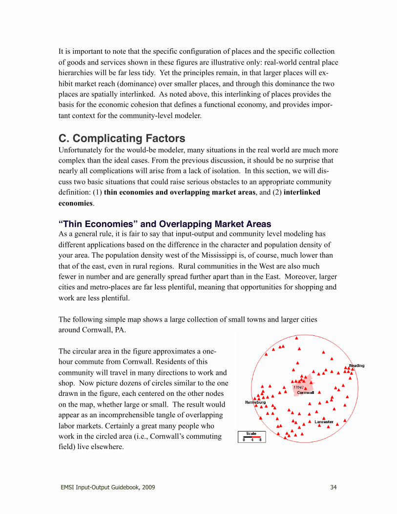
It is important to note that the specific configuration of places and the specific collection of goods and services shown in these figures are illustrative only: real-world central place hierarchies will be far less tidy. Yet the principles remain, in that larger places will ex-hibit market reach (dominance) over smaller places, and through this dominance the two places are spatially interlinked. As noted above, this interlinking of places provides the basis for the economic cohesion that defines a functional economy, and provides impor-tant context for the community-level modeler.

C. Complicating FactorsUnfortunately for the would-be modeler, many situations in the real world are much more complex than the ideal cases. From the previous discussion, it should be no surprise that nearly all complications will arise from a lack of isolation. In this section, we will dis-cuss two basic situations that could raise serious obstacles to an appropriate community definition: (1) thin economies and overlapping market areas, and (2) interlinked economies.

“Thin Economies” and Overlapping Market AreasAs a general rule, it is fair to say that input-output and community level modeling has different applications based on the difference in the character and population density of your area. The population density west of the Mississippi is, of course, much lower than that of the east, even in rural regions. Rural communities in the West are also much fewer in number and are generally spread further apart than in the East. Moreover, larger cities and metro-places are far less plentiful, meaning that opportunities for shopping and work are less plentiful.

The following simple map shows a large collection of small towns and larger cities around Cornwall, PA.

The circular area in the figure approximates a one-hour commute from Cornwall. Residents of this community will travel in many directions to work and shop. Now picture dozens of circles similar to the one drawn in the figure, each centered on the other nodes on the map, whether large or small. The result would appear as an incomprehensible tangle of overlapping labor markets. Certainly a great many people who work in the circled area (i.e., Cornwall’s commuting field) live elsewhere.


If we compare Cornwall to another example of rural western town (Grangeville, ID) the contrast is stark (below).

Cornwall (approximate population 3,500) and Grangeville (approximate population 3,200) are comparable in size, but Grangeville is isolated while Cornwall is not. Whereas the total population within a one-hour commute of Grangeville is approximately 10,000, that figure might be upwards of 1 million in Cornwall’s radius (these are very rough estimates, but good enough to make the point). The density around Cornwall creates very open markets and a web of “thin” economies with uncertain inter-community/inter-industry linkages. Even if a major event (the opening or closure of a large retail store, for example) occurred in one of these towns, the employment and other market effects would be too fleeting, easily leaking to surrounding areas.

In light of this, it does not make sense to speak of “Cornwall’s labor market” in any closed sense. Workers from Cornwall compete with workers well beyond the commute field shown in map, and similarly, job opportunities within Cornwall’s commute field are affected by business conditions beyond that field. Similar market overlap occurs in consumer and business goods and services markets.

It is therefore difficult to define or otherwise make sense of a “Cornwall economy.” One might draw the commute field shown in the figure and call this “Cornwall’s labor market,” but it would be scarcely useful due to the fact that there are so many overlapping labor markets in this same field. Narrow community boundaries, for instance Cornwall’s city limits or ZIP code, might be proposed, but this is an extremely open economy, with many goods (e.g., perhaps as common as hardware or supermarket) and services available in abundance in nearby communities. Crosshauling, which is the inflow and outflow of the same goods or services, including labor, is doubtless very prevalent.

As a result, it makes more sense to speak of a large-scale regional economy such as “the South Central Pennsylvania economy,” or perhaps a metro-area economy such as “the Harrisburg area economy.” The lesson is that because of complex trade hierarchies input-output modeling is more well suited to either larger multi-county regions around a metropolitan area, or closed economies such as can be found in the rural western states.


Interlinked EconomiesIn the previous example, we saw that community definition for the sake of modeling pur-poses, can be impossible due to extreme regional interconnection. For our next case study we turn to a much less radical situation which nonetheless exhibits a complicating lack of isolation. Consider the two communities shown in the following map: Moscow, Idaho, and Pullman, Washington.

Moscow and Pullman are located just 8 miles apart on either side of the Idaho-Washington state line. Excluding each other, these two communities are considerably iso-lated—the nearest larger cities are Lewiston-Clarkston (35 minutes), Coeur d’Alene-Post Falls (2 hours), and Spokane (2 hours), and few residents commute to or from those places. Thus the case is easily made that Moscow and Pullman represent a single, albeit bi-nodal, functioning economy: there is considerable intercommunity commuting and head-to-head competition among like businesses, e.g., restaurants, retail stores, professional services, consumer services, and so on.

That said, the existence of a state boundary means that these two communities could be modeled as a single functioning economy or as separate, though highly interlinked, com-munities. Commuting and other trade, which links these two communities, might be tracked using economic base principles, or they might be formally linked as a two-community interregional IO model (beyond the scope of this document). The choice would depend somewhat on the goals of the analysis, and how important political boundaries are in it (if taxes or local government policy are involved, modeling them separately would make more sense).

ConclusionThis chapter has presented some background theory and general advice about defining communities for modeling purposes. The advice can be summarized in three basic points:

1. Functional economic areas must take precedence over political regions when attempting to accurately model a regional economy;

2. The appropriate scale is that of a city-region; and 3. Be aware of complicating factors, which generally arise from lack of isola-

tion.


It is hoped that this chapter provides a solid foundation for the community modeler, but it should be emphasized that community definition, like region definition, is by no means a simple task that can be accomplished with only a handful of all-purpose rules. Rather, the specific geography and economics of a community or area can greatly alter a commu-nity’s boundaries for modeling purposes. Moreover, the purpose of the model being built will certainly affect the appropriate scale, and therefore the way boundaries are drawn. A model intended to examine the impact of new road construction in Idaho will likely re-quire a different focus than a model aimed at examining the impact of a mill closure in Wyoming or a commuter rail line in Pennsylvania.


io guide final - economicmodeling.com · emsi input-output guidebook, 2009 4. i. regional economics...

Documents