Iowa Bridge Backwater Software

Users Manual

Version 1.0

September 2003

Iowa DOT Bridge Backwater Program Version 1.00 Software Users Manual September 2003 Acknowledgements The Iowa Highway Research Board and the Iowa Department of Transportation funded the development of this software through Research Project TR-476, “PCVAL: A Computer Program for Valley Stage-Discharge Curves and Bridge Backwater Calculations”. Dave Claman of the Iowa DOT Office of Bridge & Structures served as the project manager. LaDon Jones was the project manager for Digital Control, Inc. The opinions, findings, and conclusions expressed in this publication are those of the author and not necessarily those of the Iowa Department of Transportation. Disclaimer: Although the Iowa Bridge Backwater (Iowa DOT Bridge Backwater Program) software and users manual have been carefully prepared and tested, the Iowa Department of Transportation and Digital Control, Inc. makes no representation or warranty regarding the accuracy, correctness, or completeness of the computer program or of the information contained in the users manual. The Iowa Department of Transportation and Digital Control, Inc. shall not be liable for any direct, indirect, consequential, or incidental damages resulting from the use of the software or the information contained herein.

Table of Contents Introduction ................................................................................................................................... 1

Applicability............................................................................................................................... 1 Installing the Software .............................................................................................................. 2 Saving/Opening Files ................................................................................................................ 2 Selecting a Printer ..................................................................................................................... 3 Exiting the Program.................................................................................................................. 3

Tutorial........................................................................................................................................... 3 Site Identification ...................................................................................................................... 3 Design-Q’s .................................................................................................................................. 3

USGS, Lara – 1987 ................................................................................................................ 4 USGS, Eash – 2001 ................................................................................................................ 5

Valley Computations................................................................................................................. 8 The Valley Cross-Section...................................................................................................... 8 The Valley Rating Curve .................................................................................................... 10 Valley Q-Stage Calculations ............................................................................................... 11 Valley Floodway .................................................................................................................. 13

Bridge Backwater .................................................................................................................... 22 Introduction ......................................................................................................................... 22 Valley Cross-Section ........................................................................................................... 23 Bridge Cross-Section........................................................................................................... 24 Bridge Piers.......................................................................................................................... 25 Bridge – River – Valley Relationship ................................................................................ 28 Compute Backwater (Without Roadway Overtopping) .................................................. 34 Backwater with Roadway Overtopping ............................................................................ 41 Road Grade Profile (For Overtopping)............................................................................. 42 Compute Backwater (With Roadway Overtopping)........................................................ 42

References .................................................................................................................................... 44 Appendix A: Copying and Pasting Values ................................................................................ 45 Appendix B: Valley Stage-Discharge Computations ............................................................... 46 Appendix C: Floodway Encroachment Limits ......................................................................... 47 Appendix D: Computing Roadway Overflow........................................................................... 49 Appendix E: Numbered Figures ................................................................................................ 50 Appendix F: Selected Information from Lara (1987) .............................................................. 58 Appendix G: USGS Regression Equations – Eash 2001 .......................................................... 61

1

Iowa Bridge Backwater Software Users Manual Introduction This manual describes how to use the Iowa Bridge Backwater software. It also documents the methods and equations used for the calculations. The main body describes how to use the software and the appendices cover technical aspects. The Bridge Backwater software performs 4 main tasks:

Design Discharge Estimation

Stream Rating Curves

Floodway Encroachment

Bridge Backwater Design discharge estimation: Design discharges are estimated by 2 methods, both from USGS reports for flood frequency in Iowa (Lara, 1987, Eash, 2001). Stream Rating Curves: Stage versus discharge relationships for streams are estimated using the Manning Equation and assuming uniform flow. This is a user friendly replacement for the PC VAL program previously used in Iowa. Floodway: Floodway encroachments can be computed, using the methods and assumptions of the Iowa Department of Natural Resources, Water Resources Division. Bridge Backwater: The estimation of backwater from bridges is a major portion of the software. The methods used by the Iowa Department of Transportation (IDOT) and Iowa Department of Natural Resources (IDNR) for Bridge Backwater Estimation are used. These methods are based on methodology from Hydraulic Design Series 1 (HDS-1), Hydraulics of Bridge Waterways, Federal Highway Administration (FHWA), 1970. Hydraulic Design Series 1 will be referenced throughout the manual, as HDS-1. Applicability

1) The intent of this program is to provide a simplified method for analysis of bridge backwater for rural structures located in areas with low flood damage potential.

2) It is recommended that this software not be used for locations with a detailed Flood Insurance Study or where the upstream floodplain has a high damage potential.

3) If the design flow inundates the superstructure, without road grade overtopping, other methodologies should be used for backwater estimation. This is a pressure flow situation and this is not modeled in the software.

2

Installing the Software The software is written in Microsoft Visual Basic 6.0. It will run under Windows 95 or newer versions (i.e. Windows 98, NT, 2000, XP). It will not run under Windows 3.11 or earlier versions of Windows. Instructions for installing the software will be included when you receive the software installation files. Saving/Opening Files When the software is installed a menu item will be placed in the Windows “Start” menu. To start the software click “Start” on the Windows Task Bar and select “Iowa Bridge Backwater”. While you are working on a project you can save the information to a file at any time using “File”, “Save”. If there is not currently an “active” file name, the “Save As” dialogue box will open, and you can select a File Name and save the current information in the program to the file. By default an extension of “ibh” is added to the file name (short for Iowa Bridge Hydraulics). You do not need to type this extension as part of the file name, it will be automatically added. I suggest you use the default extension. When you open a file, files with the default extension will be displayed automatically. After you save the data to a file, the “active” file name is automatically displayed on the top menu bar, after the program name, “Iowa Bridge Backwater v1.00”. For example, Iowa Bridge Backwater v1.00/C:\Example\Example.ich. When there is an active file name, if you click “File”, “Save” the active file is automatically updated with the current information in the program. To reduce the loss of information in the event of a software or operating system crash it is recommended you save the data to a file on a regular basis while you are working on a project. If you wish to save the information to a different file use “File”, “Save As”. To open a previously saved file, use “File”, “Open”. When you open a file any existing information in the program in replaced with the data in the file. If you are working on a project make sure you save the current information before you open a file. Selecting “File”, “New” will clear all the information from the program (it does not affect information that has been saved to a file). You might use this if you are done with a bridge design project, have saved the information to a file, and wish to start on a new project without exiting and restarting the program.

3

Selecting a Printer The software will print to the default printer. You can view or select the default printer for Windows by going to the Windows Taskbar, selecting “Start”, “Setting, “Printers” (in XP this may be “Start”, “Printers and Faxes”. You can also view or select the printer the program will print to from the software. Select “File”, “Select Printer”. This form is not used to Print from the program, but to select the printer the software will send printouts to. Exiting the Program To exit the program select “File”, “Exit”. A message box will appear for you to confirm your choice to exit. Any unsaved data will be lost when you exit the program. Data that has been saved to a file will not be lost. Tutorial The rest of the manual will go through the elements of the software, step by step. The user manual is in tutorial form, using an example problem for illustration. It is recommended you open the example problem file and follow along. If you have installed the software, select “File”, “Open” and select “Example Problem 1”. Site Identification Click “Site” on the top menu, and then click “Identification” to display the “Site Identification” form. Use this form to enter the information required to identify your site and project. You can print the information (click the “Print” button) on the form to include with your report. DATE: For a new project the current date is shown by default. You can click on the down arrow to select a date from a calendar, or type the date in directly using mm/dd/yyyy. COUNTY: Select the county from the drop down list box with the 99 counties in Iowa. ADDITIONAL COMMENTS: You can add any additional information you wish for your site. Design-Q’s Two methods for estimating design discharges are built into the software. Both are based on USGS reports on flood frequency in Iowa. One method is from the 1987 report by Lara and the other is from the 2001 report by Eash. The hydrologic regions for the 2 reports are not the same. Refer to the reports (referred below) and Appendix F and G for details on how the hydrologic regions are defined for each method. You can use these methods to estimate your design Q’s or you may enter the design Q’s directly into the software for rating curve estimation, floodway or bridge backwater calculations.

4

USGS, Lara – 1987 Click “Design-Q’s”, then click “USGS, Lara – 1987” to display the form for “USGS Flood Frequency, Lara -1987”. The discharges in this form are computed using the equations from: Method for Estimating the Magnitude and Frequency of Floods at Ungaged Sites on Unregulated Rural Streams in Iowa, U.S. Geological Survey, Water-Resources Investigation Report 87-4132, In cooperation with the Iowa Department of Transportation, Highway Division, Highway Research Board, Iowa City, Iowa, by Oscar G. Lara, 1987. This report is referred to as Lara (1987). Appendix F contains the regional equations and a map of the 5 hydrologic regions. The user is encouraged to reference a copy of the report for details on the methods and equations. Five hydrologic regions are defined for Iowa (see Appendix F and Lara-1987 for details). For each region, flood frequency and regression analysis was used to estimate equations for floods with return periods of 2, 5, 10, 25, 50 and 100 years. For example, for hydrologic region 3 the equation for the 100 year flood is:

53.0100 851AQ =

where A is the watershed drainage area in square miles, and Q100 is the 100 year discharge estimate, in cubic feet per second (cfs). As an example, if the watershed is entirely in region 3 and the drainage area is 5.2 square miles, then

2,0392,038.97)2.5(851851 53.053.0100 ≅=== AQ

You can test this example in the software by inputting 5.2 for the “Drainage area in Region 3” and clicking the “Compute Q’s” button. The Q results shown are always rounded off to whole numbers. Practical Steps To compute the Q’s using Lara -1987: For your watershed, determine the area that lies in each hydrologic region, in square miles. Type in the area in each region in the “Watershed Drainage Area” frame. If a region does not have any area in the watershed, you can leave the entry blank or input 0. The software will determine the “Total Drainage Area”, you do not type in the “Total Drainage Area”. Click the “Compute Q’s” button. The software will determine the “Total Drainage Area” from the values you entered for the Regions, then compute the estimated discharge and display the results in the grid under the “Q” column.

5

Copying the Values You can copy the values in the Q table for pasting into other sections of the software or into other programs. See appendix A for instructions on copying and pasting. You can not paste values into the Q grid in this form. Multiple Region Calculation Method The regression equations in Lara (1987) are defined for individual regions. If your watershed contains multiple regions the software computes the Q’s using a weighted area approach. For example, suppose your watershed consists of: 4 squares miles in region 1, and 12 square miles in region 2, and you wish to find the Q50 estimate. The total drainage area is 16 square miles. First, the Q50 for each region is determined using the total drainage area. For region 1:

cfsAQ 7917)16(15001500 6.060.050 ===

For region 2:

cfsAQ 4434)16(10201020 53.053.050 ===

The Q is determined by adding together the results from each region, weighted by the fraction of total area in the region,

cfsQ 53054434*)16/12(7917*)16/4(50 =+= You can test this example using the software. USGS, Eash – 2001 In addition to the Lara (1987) estimates, the software implements the results from the most recent report: Techniques for Estimating Flood Frequency Discharges for Streams in Iowa, U.S. Geological Survey, Water Resources Investigations Report 00-4233, David A. Eash, Iowa City Iowa, 2001. The software implements the methods for ungaged sites on ungaged streams. Appendix G contains the regional equations for the hydrologic regions defined by Eash, and 2 maps defining the regions. For more detailed information see the above-mentioned report (Eash, 2001). You can download a copy of the Flood-Frequency report over the Internet, in PDF format, from the web site: http://webdiaiwc.cr.usgs.gov/pubs/online.html

6

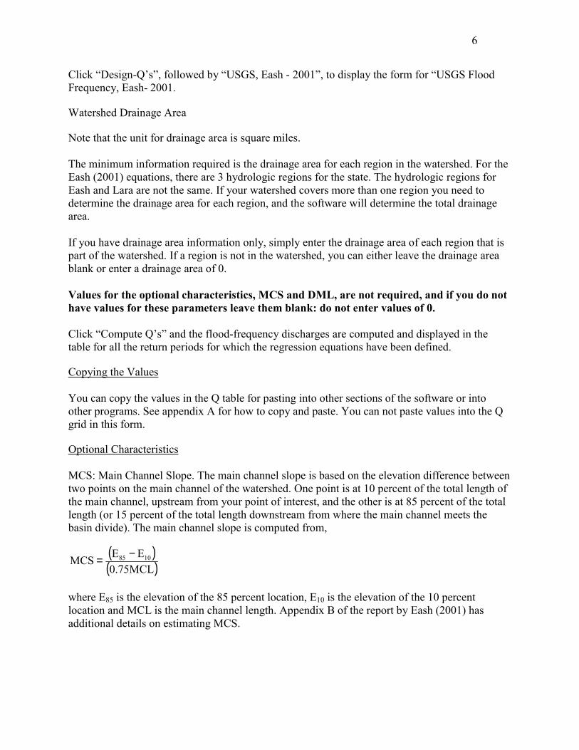
Click “Design-Q’s”, followed by “USGS, Eash - 2001”, to display the form for “USGS Flood Frequency, Eash- 2001. Watershed Drainage Area Note that the unit for drainage area is square miles. The minimum information required is the drainage area for each region in the watershed. For the Eash (2001) equations, there are 3 hydrologic regions for the state. The hydrologic regions for Eash and Lara are not the same. If your watershed covers more than one region you need to determine the drainage area for each region, and the software will determine the total drainage area. If you have drainage area information only, simply enter the drainage area of each region that is part of the watershed. If a region is not in the watershed, you can either leave the drainage area blank or enter a drainage area of 0. Values for the optional characteristics, MCS and DML, are not required, and if you do not have values for these parameters leave them blank: do not enter values of 0. Click “Compute Q’s” and the flood-frequency discharges are computed and displayed in the table for all the return periods for which the regression equations have been defined. Copying the Values You can copy the values in the Q table for pasting into other sections of the software or into other programs. See appendix A for how to copy and paste. You can not paste values into the Q grid in this form. Optional Characteristics MCS: Main Channel Slope. The main channel slope is based on the elevation difference between two points on the main channel of the watershed. One point is at 10 percent of the total length of the main channel, upstream from your point of interest, and the other is at 85 percent of the total length (or 15 percent of the total length downstream from where the main channel meets the basin divide). The main channel slope is computed from,

( )( )MCL75.0

EEMCS 1085 −=

where E85 is the elevation of the 85 percent location, E10 is the elevation of the 10 percent location and MCL is the main channel length. Appendix B of the report by Eash (2001) has additional details on estimating MCS.

7

A report by Eash (2003) has graphs for the “Main-Channel Slope of Selected Streams in Iowa for Estimation of Flood-Frequency Discharges”. See the references for more details on the report. A copy of the report can be downloaded from http://webdiaiwc.cr.usgs.gov/pubs/online.html DML is the fraction of the watershed area in the Des Moines Lobe landform region. You enter the area of the watershed, if any, in the Des Moines Lobe landform region and the software will calculate the fraction of the watershed in the Des Moines Lobe region. Note that if you choose to measure and input the optional parameters (MCS, DML) their values are based on the entire watershed. For example, if the watershed has areas in region 1 and region 2, the MCS is the MCS for the entire watershed, not the MCS for one of the regions. Regional Regression Equations For region 1 there is only one set of regression equations, with drainage area as the only parameter. MCS and DML values have no effect on discharge estimates for region 1. For region 2 there are two sets of equations, a one-variable set of equations using drainage area only and a three-variable set of equations using drainage area, MCS and DML. The software automatically selects the equations to use based on the parameters you have input. If you have input a drainage area for region 2, along with values for MCS and DML, the software will use the three-variable equations for region 2. Otherwise, the one-variable equations are used. Note that to use the three variable equations you must input a value for DML (even if the value is zero). If you leave DML blank the one variable equation is used, even if you have input a value for MCS. However, if you do not actually know what the DML or MCS is, you should leave them empty or blank. For region 3 there are two sets of equations, a set of one-variable equations using drainage area only, and a set of two-variable equations using drainage area and MCS. If your watershed has a drainage area in region 3 the software will use the two-variable equations if you have entered a value for MCS (> 0), otherwise the one-variable equations will be used. Appendix G contains the regional equations. Multiple-region watershed If your watershed has drainage areas in more than one region the watershed discharge is computed using an area-weighted average of the regional runoff estimates,

it

i QDADAQ �=

where Qi is the runoff estimate for region i (computed using the total watershed drainage area), DAi is the drainage area for region i and DAt is the total watershed drainage area. This is the same methodology as that used for Lara (1987).

8

Valley Computations The Valley Cross-Section The valley cross-section information is used to generate valley rating curves, and to estimate discharge versus depth for floodway encroachment and for bridge backwater estimation. All the computations (except for design Q estimation) in the software require a valley cross-section. Note that for bridge backwater calculations the valley cross-section should be a “typical” or representative cross-section for the valley in the vicinity of the bridge. You may need to edit or modify the measured cross-section if it contains features (i.e. local scour hole) that are not representative of the typical valley cross-section. You can reach the valley cross-section form two ways. You can Click “Valley”, then “Valley Cross-Section”, or click “Backwater”, then “Valley Cross-Section” to display the “Valley Cross-Section” form. Both methods display the same form. You can reach it from 2 locations for convenience, in case you are doing a valley rating curve or a bridge backwater, but not both. You use this form to enter the data describing the valley cross-section. Channel Slope: Channel Slope is the slope of the channel bottom in the direction of flow. Always enter the slope as a positive (>0) value. Valley Cross-Section Data: Use the grid or table on the left of the form to enter the valley cross-section data. Station values are not in transportation station notation. For example, if the station location is 1256 feet, you must enter 1256, not 12+56. Normally, the station values are entered left to right assuming you are looking upstream. However, they can be entered with another orientation, but if you use the bridge backwater section, the valley cross-section and bridge cross-section must use the same orientation. Station values must be entered in ascending (increasing) order, although the first station does not need to be zero, and can be negative. Elevation is the elevation of the channel bottom at the station. The first station must have a Manning n value. Manning n values apply from the station they are entered at until another Manning n value is entered. Hence, you do not need to enter Manning n values for each station. You need to enter a Manning n for the first station and then at each station where there is a change in Manning n value. The example problem only has Manning n values where there is a change in value. Overbanks

9

The “Left Overbank Station” and “Right Overbank Station” only affect the calculations for Floodway Encroachment. However, you must enter a Left Overbank and Right Overbank Station even if you are not doing floodway encroachment. Overbank stations are sometimes called top of bank (TOB) stations. The left overbank station must have a station value less than the right overbank station. The over bank station does not have to be equal to one of the valley stations. You can use an overbank station between valley stations and the software will interpolate the valley cross-section data to find the valley bottom elevation at that point. Inserting Rows If you need to insert rows in the grid place the mouse cursor over the grid and click the right mouse button. On the pop-up menu click “Insert Rows”. Enter the number of rows you wish to insert, and select whether you want the insertion before or after the current row. Deleting Rows To delete rows of data, first select the rows you want to delete. To select rows, place the mouse cursor on the grid, then click the left mouse button and hold it down while you drag over the rows you want to delete. Release the left mouse button and click the right mouse button. Select “Delete Selected Rows” from the pop-up menu. You will then be asked to confirm that you want to delete the selected rows. You can also select rows by clicking on the click, pressing and holding down the “Shift” key, and using the arrow keys. Deleting Data If you need to delete data from the grid, without inserting or deleting rows, select the information you wish to delete, then press the Delete (Del) key on your keyboard. To select information you can press and hold down the left mouse button and drag the mouse over the area you wish to select, then release the mouse button. Or use the “Shift” and arrow keys. Copying and Pasting Data You can copy and/or paste data to the grid. See appendix A. An alternative to Ctrl-C and Ctrl-V is to right click when the mouse cursor is on the grid and select “Copy” or “Paste” from the pop-up menu. You need to select the area you wish to copy from or paste to before you click “Copy” or “Paste” from the pop-up menu. Printing the Valley Cross-Section Data To send the Valley Cross-Section Data to the printer, simply click the “Print the Data” button at the top left of the form. Plotting the Valley Cross-Section

10

Click the “Plot the Cross-Section” button to plot the Valley cross-section. The Manning n values and their range of coverage are shown at the top of the plot. The channel bottom is shown with a red line. The Left Overbank Station is shown as “LOB” and the Right Overbank Station is shown as “ROB”. The “O” in LOB is centered at the Left Overbank Station and the “O” in ROB is centered at the Right Overbank Station. The scaling for the x and y axes are chosen automatically by the software. The right vertical axis shows depth, computed treating the lowest elevation in the valley cross-section data as a depth of 0. Printing the Valley Cross Section To send a copy of the valley cross-section to the printer click the “Print the Plot” button. The scaling and placement of the cross-section is automatically selected by the software. The plot is always printed with a landscape format. The Valley Rating Curve Click “Valley”, “Valley Rating Curve” to display the “Rating Curve for Valley Cross-Section” form. You can use this form to generate a table and plot of discharge versus water surface elevation (and depth), a so-called Rating Curve. The water surface elevation is called the “Stage”. For a given Stage (water surface elevation) the discharge (Q) is computed. The computations use the channel slope and valley cross-section information you have entered in the “Valley Cross-Section” form, discussed above. The only parameters you need to enter in this form are the “Starting Stage”, “Ending Stage” and the “Step Size”. The flowrates are computed for water surface elevations from the “Starting Stage” to the “Ending Stage”, in increments of “Step Size”. For example, if you enter a “Step Size” of 1 foot the flowrate (Q) will be computed for the “Starting Stage” and at one-foot elevation increments of stage until the “Ending Stage” is reached. The computation stages do not have to fall evenly on the “Ending Stage”. The discharge for the Ending Stage will be computed, regardless. For example, if you have: Starting Stage = 100.0 Ending Stage = 103.5 Step Size = 1.0 The discharge will be computed for 100.0, 101.0, 102.0, 103.0 and 103.5 After you have entered a “Starting Stage”, “Ending Stage” and “Step Size”, click the “Compute/Plot Rating Curve” button to compute the rating curve. This will fill the table with the results of the computations and also plot discharge (Q) versus water surface elevation (stage) and water surface depth. The depth is the depth of water above the lowest elevation in the valley cross-section.

11

You can send a copy of the table to the printer using the “Print the Data” button, and print a copy of the plot using the “Print the Plot” button. The table results and plot are not saved when you save the data to a file, but all the information needed to reproduce the results are saved. So if you open a previously saved file, you only need to click “Compute/Plot Rating Curve” to reproduce the results. The rating curve table shows: Stage: The elevation of the water surface. Depth: Depth of the water surface. The depth of water above the lowest elevation in the valley cross-section. Q: The flowrate or discharge, computed using the Manning Equation. Velocity: The average velocity, computed from the discharge (Q) divided by the cross-sectional area of flow (Area). Area: The cross-sectional area of flow at the given stage. Conveyance: The conveyance at the given stage, which can be found from Q divided by S0.5. The computations use the Manning Equation,

nSAR49.1Q

2/13/2

=

where n is the Manning coefficient, A is the cross-sectional area of flow, R is the hydraulic radius and S is the slope of the energy grade line. The slope of the energy grade line (S) is assumed equal to the channel slope (the value you entered for channel slope in the “Valley Cross-Section” form). The Manning Equation can be written as,

2/1KSQ = where K is the conveyance,

2/1

3/249.1SQ

nARK ==

Appendix B contains additional information on the Stage-Discharge computations. Valley Q-Stage Calculations

12

Click “Valley”, “Valley Q-Stage Calcs” to display the “Stage-Q Calculations for Valley Cross-Section” form. You can use this form to compute the stages for discharges you select. This may be more convenient than interpolating values from a rating curve. Or you can have the discharges computed for stages you select. All computations use the Valley Cross-Section and Channel Slope information you have entered in the “Valley Cross-Section” form. The Manning equation is used, and it is assumed the slope of the energy grade line is equal to the slope of the channel bottom (uniform flow). Calculator Pad The grid on the left is a “calculator” pad you can use as needed. The computation options are shown in the “Select Calculation Option” frame below the grid. For example, if you enter Q values in the “Q” column, set the option below the grid to “Given Q, Find Stage and Depth”, then click “Compute”, the software will compute the water surface stage and depth for the Q’s in the “Q” column, and display the computed Stages and Depths in the appropriate columns. If the option is set to “Given Stage, Find Q and Depth”, when “Compute” is clicked the Stage values will be read from the table, and the computed Q’s and Depths for the given Stages will be displayed in the table. If the option is set to “Given Depth, Find Q and Stage”, when “Compute” is clicked the Depth values will be read from the table, and the computed Q’s and Stages for the given Depths will be displayed in the table. You can type values directly into the table, or copy Q values into the table (See Appendix A for additional information about copying). You can also use Ctrl-C and Ctrl-V to copy/paste to and from this table. For example, you could go to the Eash-2001 Design Q table, copy the values to the clipboard using Ctrl-C, then select the cells in the “Return Period” and “Q” column and paste the values in using “Ctrl-V” If you click on the table with the right mouse button you can also use the pop-up menu to add or delete rows, or copy and paste. Printing the Results To print the results in the calculator pad grid, click the “Print the Table” button in the “Select Calculation Option” frame below the grid. Plotting/Printing a Selected Stage To plot a selected stage, you must first select the row in the calculator pad with the stage value you want to plot. To select a row in the grid, simply click on any column in the row with the left mouse button. Then click “Plot Selected Stage”. This will produce a plot of the valley cross-

13

section with the stage shown with a blue line, and the notation “Valley Stage”. To send a copy of the plot to the printer, click “Print the Plot”. All the plot does is take the stage value in the selected row of the grid and plot it against the valley cross-section. It also displays the other information in the row (Return Period, Q, and Depth) on the plot. It is assumed that the data in the table was generated using the software (using “Compute”), which means it is assumed it was generated using the valley cross-section entered into the software. Valley Floodway Click “Valley”, then “Valley Floodway” to display the “Floodway for the Valley Cross-Section” form. This form can used to estimate the encroachment floodway limits for the valley. These limits are established by allowing encroachment on the flood plain of a stream, subject to the maximum backwater from encroachment not exceeding the stage for the natural conditions for a 100 year flood by more than an allowable limit (usually 1 foot). The methods for floodway encroachment, and regulation of floodway encroachment, are defined as part of the floodplain management program of the Water Resource Section of the Iowa Department of Natural Resources. Appendix C is a copy of information from the Water Resource Section used as the basis for the computations in this form. You are encouraged to review this information. The floodway encroachment is applied to the valley cross-section. If you have not already done so, you will need to first enter a valley cross-section (“Valley”, Valley Cross-Section”). Design Q’s You will need to enter your floodway Design Q’s in the Design Q’s grid at the top left of the form. If you have entered or computed the appropriate values at other locations in the software, you can copy the values (Ctrl-C) and paste them into this grid (Ctrl-V), or type the values in directly. Normally, the 100 year flood discharge is used as the Design Q. Auto Mode In “Auto Mode” the software automatically finds the encroachment limits that meet the allowable rise due to encroachment. You need to enter the “Allowable rise due to encroachment”. This is normally 1.0 foot, and this is the default value. “Auto Mode” is specified by selecting “Find Encroachment Stations (Auto Mode)” as the “Specify Computation Option”. With this selection, click the “Compute Floodway” button to have the software find the encroachment limits for the Design Q’s, subject to the allowable rise. Floodway Results for Auto Mode

14

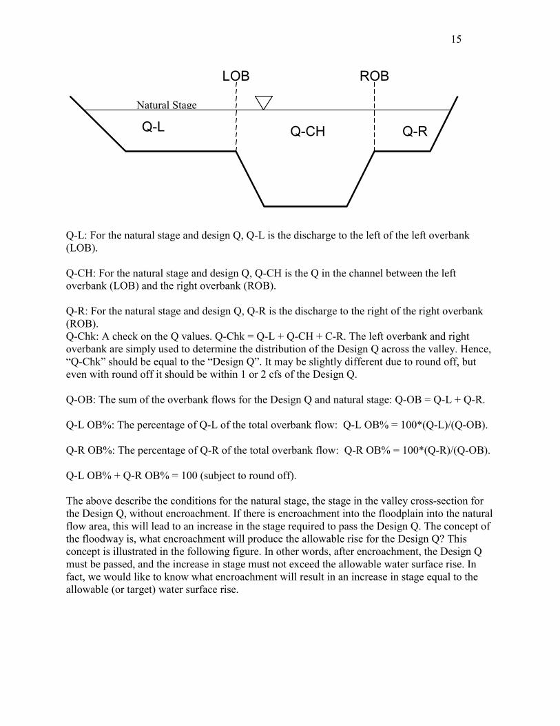
We will use the example problem to discuss the floodway results. After you click “Compute Floodway”, the results are shown in the frame and grid beneath the button. The “Computation Option Used” shows the criteria used for the floodway results. For “Auto Mode”, the “Mode” will be “Automatic”. The “Allowable Rise” used for the computations are shown. The grid (table) shows the results of the computations, in column format: that is, a single column shows the results for a single design Q. There is a column for each design Q in the design Q grid. We will discuss the results shown in the table, using the results for the example problem for the 100 year flood (Return Period = 100, Design Q = 21800). Again, all computations are applied to the valley cross-section. The rows in the table are: Return Period: The return period, in years. This is simply a copy of the value you entered in the “Design Q’s” grid. Design Q: The design Q, in cfs. This is simply a copy of the value you have entered in the “Design Q’s” grid. Natural Stage: This is the computed water surface elevation (stage), for the “Design Q” applied to the valley cross-section, with no encroachment. This computation uses Manning’s equation, with the assumption of steady, uniform flow. This is the same methodology used for computing the valley rating curve. The floodway stage is actually computed to 1/1000 of a foot (0.001), but the solution is rounded off to 1/100 of a foot. Natural Depth: The depth of the natural stage above the lowest elevation of the valley cross-section. The notation that follows is that of the Water Resource Section of the IDNR, as shown in the figure below.

15

LOB ROB

Natural Stage

Q-L Q-CH Q-R

Q-L: For the natural stage and design Q, Q-L is the discharge to the left of the left overbank (LOB). Q-CH: For the natural stage and design Q, Q-CH is the Q in the channel between the left overbank (LOB) and the right overbank (ROB). Q-R: For the natural stage and design Q, Q-R is the discharge to the right of the right overbank (ROB). Q-Chk: A check on the Q values. Q-Chk = Q-L + Q-CH + C-R. The left overbank and right overbank are simply used to determine the distribution of the Design Q across the valley. Hence, “Q-Chk” should be equal to the “Design Q”. It may be slightly different due to round off, but even with round off it should be within 1 or 2 cfs of the Design Q. Q-OB: The sum of the overbank flows for the Design Q and natural stage: Q-OB = Q-L + Q-R. Q-L OB%: The percentage of Q-L of the total overbank flow: Q-L OB% = 100*(Q-L)/(Q-OB). Q-R OB%: The percentage of Q-R of the total overbank flow: Q-R OB% = 100*(Q-R)/(Q-OB). Q-L OB% + Q-R OB% = 100 (subject to round off). The above describe the conditions for the natural stage, the stage in the valley cross-section for the Design Q, without encroachment. If there is encroachment into the floodplain into the natural flow area, this will lead to an increase in the stage required to pass the Design Q. The concept of the floodway is, what encroachment will produce the allowable rise for the Design Q? This concept is illustrated in the following figure. In other words, after encroachment, the Design Q must be passed, and the increase in stage must not exceed the allowable water surface rise. In fact, we would like to know what encroachment will result in an increase in stage equal to the allowable (or target) water surface rise.

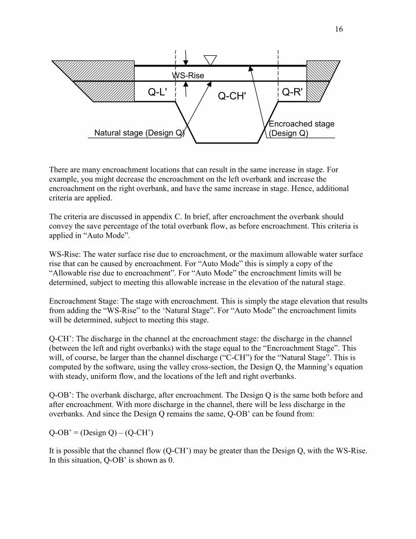
16

WS-Rise

-L' -R'Q QQ-CH'

Encroached stage(Design Q) Natural stage (Design Q)

There are many encroachment locations that can result in the same increase in stage. For example, you might decrease the encroachment on the left overbank and increase the encroachment on the right overbank, and have the same increase in stage. Hence, additional criteria are applied. The criteria are discussed in appendix C. In brief, after encroachment the overbank should convey the save percentage of the total overbank flow, as before encroachment. This criteria is applied in “Auto Mode”. WS-Rise: The water surface rise due to encroachment, or the maximum allowable water surface rise that can be caused by encroachment. For “Auto Mode” this is simply a copy of the “Allowable rise due to encroachment”. For “Auto Mode” the encroachment limits will be determined, subject to meeting this allowable increase in the elevation of the natural stage. Encroachment Stage: The stage with encroachment. This is simply the stage elevation that results from adding the “WS-Rise” to the ‘Natural Stage”. For “Auto Mode” the encroachment limits will be determined, subject to meeting this stage. Q-CH’: The discharge in the channel at the encroachment stage: the discharge in the channel (between the left and right overbanks) with the stage equal to the “Encroachment Stage”. This will, of course, be larger than the channel discharge (“C-CH”) for the “Natural Stage”. This is computed by the software, using the valley cross-section, the Design Q, the Manning’s equation with steady, uniform flow, and the locations of the left and right overbanks. Q-OB’: The overbank discharge, after encroachment. The Design Q is the same both before and after encroachment. With more discharge in the channel, there will be less discharge in the overbanks. And since the Design Q remains the same, Q-OB’ can be found from: Q-OB’ = (Design Q) – (Q-CH’) It is possible that the channel flow (Q-CH’) may be greater than the Design Q, with the WS-Rise. In this situation, Q-OB’ is shown as 0.

17

Q-L’: The left overbank flow, after encroachment. By policy, this is to have the same percentage, or fraction, of overbank flow prior to encroachment (Q-L OB%). Q-L’ is computed from: Q-L’ = (Q-OB’) * (Q-L OB%)/100 = (Q-OB’) * (Q-L)/((Q-L)+(Q-R)) Q-R’: The right overbank flow, after encroachment. By policy, this is to have the same percentage, or fraction, of overbank flow prior to encroachment (Q-R OB%). Q-R’ is computed from: Q-R’ = (Q-OB’) * (Q-R OB%)/100 = (Q-OB’) * (Q-R)/((Q-L)+(Q-R)) Q-L’ OB%: The percentage of left overbank flow (of total overbank flow), after encroachment. This provides an easy check on the criteria. Q-L’ OB % should be equal to Q-L OB%. The left overbank fraction of total overbank flow is set, by policy, to be equal before and after encroachment. Q-L’ OB% is computed from Q-L’ OB% = 100*(Q-L’)/ (Q-OB’) Q-R’ OB%: The percentage of right overbank flow (of total overbank flow), after encroachment. This provides an easy check on the criteria. Q-R’ OB % should be equal to Q-R OB%. The right overbank fraction of total overbank flow is set, by policy, to be equal before and after encroachment. Q-R’ OB% is computed from Q-R’ OB% = 100*(Q-R’)/ (Q-OB’) Q’-Chk: A check on the discharges before and after encroachment. Q’-Chk = (Q-L’) + (Q-CH’) + (Q-R’) This should be, under normal conditions, equal to the Design Q. The exception is when the new channel discharge (Q-CH’) is greater than the original Design Discharge. Finding the Encroachment Limits Having defined the discharges required in the overbanks (Q-L’ and Q-R’) after encroachment, the real work is in finding the left and right encroachment locations, such that the target discharges occur. This is done by the software by iteration. Encroachment locations are selected and adjusted until the discharge between the encroachments and overbanks match the target discharges (Q-L’ and Q-R’). Left Encroachment Limit: The station location where the discharge between this station and the left overbank is equal to (Q-L’). This is found by iteration. For an assumed left encroachment station the discharge between that station and the left overbank is computed and compared to the target discharge (Q-L’). The left encroachment limit iteration starts at the left overbank and is then moved to the left until the discharge matches the target discharge (Q-L’). Q-L’ Calc.: The actual computed discharge between the Left Encroachment Limit and the Left Overbank, rounded to the nearest cfs. This should match Q-L’. Any difference should be no more than a few cfs, due to round-off.

18

Right Encroachment Limit: The station location where the discharge between this station and the right overbank is equal to (Q-R’). This is found by iteration. For an assumed right encroachment station the discharge between that station and the right overbank is computed and compared to the target discharge (Q-R’). The right encroachment limit iteration starts at the right overbank and is then moved to the right until the discharge matches the target discharge (Q-R’). Q-R’ Calc.: The actual computed discharge between the Right Encroachment Limit and the Right Overbank, rounded to the nearest cfs. This should match Q-R’. Any difference should be no more than a few cfs, due to round-off. Left Floodway Width: The horizontal distance between the Left Encroachment and the Left overbank. Left Floodway Width = Left Overbank Station – Left Encroachment Station. The distance to the left of the left overbank that should not be encroached. RightFloodway Width: The horizontal distance between the Right Encroachment and the Right overbank. Right Floodway Width = Right Encroachment Station - Right Overbank Station. The distance to the right of the right overbank that should not be encroached. Printing the Floodway Results To send a copy of the floodway results to the printer, click “Print the Data”. This will print all results in the table, in a tabular form. Plotting the Floodway Results To plot the floodway, you must first select the results you wish to plot. To select a result, simply click with the left mouse button on the column in the grid for which you wish to plot the results. You may click on any row in your column of interest. Then click “Plot Floodway”. This will display the “Valley Floodway Plot” form, which provides a visual representation of the results. The valley cross-section is shown, with the channel bottom in red. The top of the plot shows the distribution of Manning’s n values. The left overbank (LOB) is shown with the “O” in LOB centered on the left overbank location. The right overbank (ROB) is shown with the “O” in ROB centered on the right overbank location. The “Natural Stage” is shown as a blue line. The red horizontal line above the “Natural Stage” shows the “Encroached Stage”. The vertical green lines show encroachment limits. The left vertical green line shows the “Left Encroachment Limit”. The station for the “Left Encroachment Limit” is shown at the top of the line. The right vertical green line shows the “Right Encroachment Limit”. The station for the “Right Encroachment Limit” is shown at the top of the line. To send a copy of the plot to the printer, click “Print the Plot”. To return to the floodway calculation form, click “Close”.

19

Manual Mode for Floodway Calculations In “Auto Mode”, for the Design Q the encroachment locations that will produce a target rise in the stage are determined, subject to the overbank percentages being the same for the natural and encroached stage. In Manual mode, you enter encroachment locations and the increase in stage and overbank percentages are determined. Manual mode may be useful to estimate the stage increase from a proposed or existing encroachment. To use manual mode: Enter the Floodway Design Q’s in the grid at the top left. Enter the “Allowable rise due to encroachment”. Note that this number can represent your allowable target. The actual rise will be computed, based on the encroachment stations you enter. Select “Input Encroachment Stations (Manual Mode)” for “Specify Computation Option”. Enter the “Left Encroachment Station”. Enter the “Right Encroachment Station”. Click “Compute Floodway”. The rise and overbank percentages are computed for the encroachment stations you have entered. The “Computation Option Used” shows that the results are from “Manual” mode and the encroachment stations that where used for the computations. Keep in mind that for Manual mode, the calculations are based on the encroachment stations you entered. Whereas for Auto Mode, the encroachment stations that meet the allowable rise and overbank criteria are found by the software. The rows in the results table for manual mode are: Return Period: the return period, in years. This is simply a copy of the value you entered in the “Design Q’s” grid. Design Q: the design Q, in cfs. Again, this is simply a copy of the value you have entered in the “Design Q’s” grid. Natural Stage: This is the computed water surface elevation (stage), for the “Design Q” applied to the valley cross-section. This computation uses Manning’s equation, with the assumption of steady, uniform flow. This is the same methodology used for computing the valley rating curve.

20

Natural Depth: The depth of the natural stage, measured above the lowest elevation in the valley cross-section. Q-L: For the natural stage and design Q, Q-L is the discharge to the left of the left overbank (LOB). Q-CH: For the natural stage and design Q, Q-CH is the Q in the channel, which is between the left overbank (LOB) and the right overbank (ROB). Q-R: For the natural stage and design Q, Q-R is the discharge to the right of the right overbank (ROB). Q-Chk: A check on the Q values. Q-Chk = Q-L + Q-CH + C-R. The left overbank and right overbank are simply used to determine the distribution of the Design Q. Hence, “Q-Chk” should be equal to the “Design Q”. It may be slightly different due to round off, but even with round off it should be within 1 or 2 cfs of the Design Q. Q-OB: The sum of the overbank flows for the Design Q and natural stage: Q-OB = Q-L + Q-R. Q-L OB%: The percentage of Q-L of the total overbank flow: Q-L OB% = 100*(Q-L)/(Q-OB). Q-R OB%: The percentage of Q-R of the total overbank flow: Q-R OB% = 100*(Q-R)/(Q-OB). Q-L OB% + Q-R OB% = 100 (subject to round off). The above describe the conditions for the natural stage, the stage in the valley cross-section for the Design Q, without encroachment. The encroached results are based on the encroachment locations you have entered. WS-Rise: The water surface rise due to encroachment limits you have entered. This is the computed water surface rise for the manual encroachment limits. It will not be, except by chance, equal to the “Allowable Rise”. For manual mode, using the encroachment limits you have entered, the water surface rise is the increase in stage that will result in the Design Q as the discharge between the left and right encroachment stations. Encroachment Stage: The stage with encroachment. This is simply the stage elevation that results from adding the “WS-Rise” to the ‘Natural Stage”. At the encroachment stage, the discharge is equal to the design Q between the left and right encroachment stations. Q-CH’: The discharge in the channel at the encroachment stage: the discharge in the channel (between the left and right overbanks) with the stage equal to the “Encroachment Stage”. This will, of course, be larger than the channel discharge (“C-CH”) for the “Natural Stage”. This is computed by the software, using the valley cross-section, the Design Q, the Manning’s equation with steady, uniform flow, and the locations of the left and right overbanks.

21

Q-OB’: The overbank discharge, after encroachment. The Design Q is the same both before and after encroachment. With more discharge in the channel, there will be less discharge in the overbanks. And since the Design Q remains the same, Q-OB’ can be found from: Q-OB’ = (Design Q) – (Q-CH’) Q-L’: The left overbank flow, after encroachment. The discharge between the left encroachment station and the left overbank. For manual mode, this is computed. Q-R’: The right overbank flow, after encroachment. The discharge between the left encroachment station and the left overbank. For manual mode, this is computed. Q-L’ OB%: The percentage of left overbank flow (of total overbank flow), after encroachment. For manual mode, it is not required that this be equal to Q-L OB%. You can compare this value to Q-L OB% to see how the left overbank percentage has changed for the encroachment stations you have entered. Q-R’ OB%: The percentage of right overbank flow (of total overbank flow), after encroachment. For manual mode, it is not required that this be equal to Q-R OB%. You can compare this value to Q-R OB% to see how the right overbank percentage has changed for the encroachment stations you have entered. Q’-Chk: A check on the discharges before and after encroachment. Q’-Chk = (Q-L’) + (Q-CH’) + (Q-R’) This should be equal to the Design Q, within round-off (at most a couple of cfs). Left Encroachment Limit: In manual mode, this is simply the value you entered as the left encroachment station. Q-L’ Calc.: The actual computed discharge between the Left Encroachment Limit and the Left Overbank, rounded to the nearest cfs. This should match Q-L’. In manual mode, this is somewhat redundant. Right Encroachment Limit: In manual mode, this is simply the value you entered as the right encroachment station. Q-R’ Calc.: The actual computed discharge between the Right Encroachment Limit and the Right Overbank, rounded to the nearest cfs. This should match Q-R’. In manual mode, this is somewhat redundant. Left Floodway Width: The horizontal distance between the Left Encroachment and the Left overbank. Left Floodway Width = Left Overbank Station – Left Encroachment Station. Right Floodway Width: The horizontal distance between the Right Encroachment and the Right overbank. Right Floodway Width = Right Encroachment Station - Right Overbank Station.

22

Bridge Backwater Introduction When a bridge is placed in a floodway, normally, to keep the cost down, it does not span the entire floodplain. Hence, under flood conditions, say the 100 year flood, the bridge opening is likely to restrict the area of flow, compared to the natural floodplain (See Figure 1 and Figure 2 in Appendix E). Under such conditions we need to estimate the backwater caused by the bridge, and the flow conditions through the bridge, in order to protect both the upstream area from excessive flooding (above natural conditions) and, perhaps more importantly, to insure the bridge will not be damaged. The purpose of the Bridge Backwater section of the software is to estimate the backwater due to a bridge and the flow conditions through the bridge (depth, velocity, etc.). The software implements the methodology employed by the Iowa Department of Transportation and the Iowa Department of Natural Resources for these computations. These methodologies are based on the reference: Hydraulics of Bridge Waterways, Hydraulic Design Series No. 1, published by the U.S. Department of Transportation, Federal Highway Administration, Washington, D.C., 1970. This reference is often referred to as “HDS-1” from “Hydraulic Design Series No. 1”, and we will also refer to it as HDS-1. The user who performs bridge backwater computations is encouraged to obtain a copy of this reference and read it. It makes for fascinating reading. You can download a copy of HDS-1 in pdf format from the FHWA at the link http://www.fhwa.dot.gov/bridge/hydpub.htm. The backwater of bridges is complicated. Trying to solve the full 3-dimensional flow equations is difficult. HDS-1 is an approximate method based on theory, laboratory experiments and field studies, and requires much less information than would be required for a full 3-dimensional model. On the other hand, given the uncertainties in modeling real world processes (what is the design Q?, what are the Manning’s n values?, etc.), using more sophisticated models would not guarantee a more accurate solution. When the uncertainty in the magnitude of the 100 year flood can easily be 30%, some approximations in the solution of the backwater seem reasonable. The information required for estimating the bridge backwater includes: The valley cross-section. This is the natural cross-section of the channel and floodplain, without the bridge. This cross-section is typically taken 100 or more feet downstream or upstream of the proposed bridge location. At a proposed bridge location, the valley cross-section must be surveyed outside the earthwork for the bridge. The valley cross-section should represent a “typical” cross-section in the vicinity of the bridge. If your valley cross-section contains features that are not typical (i.e. a scour hole, etc.) you may need to edit the cross-section data. The bridge cross-section. The cross-section at the bridge, taken along the road centerline. This is a survey of the bridge opening. Bridge abutments and piers. The type of bridge abutments and the types and locations of the piers need to be defined.

23

Location of the bridge opening with respect to the valley cross-section. The horizontal and vertical location of the bridge opening with respect to the valley cross-section must be defined. The distribution and amount of flow that must contract to pass through the bridge opening has a major, usually the largest, impact on the magnitude of the backwater. Bridge to river skew. The angle of the river flow direction with respect to the bridge opening, abutments and piers will affect the backwater. The Design Discharges (Q). All the forms for bridge backwater are under the “Backwater” menu at the top of the main form. Although you can access the forms in any order, normally you would work down the menu. In order to compute the bridge backwater, you must have entered in the required information for the: “Valley Cross-Section”, “Bridge Cross-Section”, “Bridge Piers “Bridge-River-Valley Relationship” You can then compute the bridge backwater, using the menu item, “Compute Backwater (Without Roadway Overtopping)” If you wish to “Computer Backwater (With Roadway Overtopping)”, you will also need to define the “Road Grade Profile (For Overtopping). Valley Cross-Section Click “Backwater”, then “Valley Cross-Section” to display the “Valley Cross-Section” form. There is only one valley channel cross-section form in the software. The same form is displayed when you select “Valley”, “Valley Cross-Section”. The valley cross-section data form can be reach from both places for convenience. You may have already entered the appropriate valley cross-section data. If not, you need to do it here. Again, I want to emphasize the cross-section represents the natural channel conditions that exist without the bridge, and should be “typical” of the valley in the vicinity of the bridge. Entering information into this form has already been covered in The Valley Cross-Section, under Valley Computations. Please refer to this section, if you need additional information on using this form for entering you valley cross-section data (it is the same form).

24

Bridge Cross-Section Click “Backwater”, then “Bridge Channel Cross-Section” to display the “Bridge Cross-Section” form. This is where you enter the information needed to define the water way opening through the bridge. In the grid (table) to the left of the form, enter the station and elevations defining the sides and bottom of the bridge opening, along the centerline of the roadway. You should start at the top of the left bridge abutment (looking upstream) at the bottom of the bridge deck and define the bottom elevation of the bridge opening to the top of the right bridge abutment at the bottom of the bridge deck. Bridge Deck Enter the station and elevation for the bottom of the bridge deck at the left and right abutments, in the “Bottom of Bridge Deck Location” frame. Use the same stationing origin as used for the bridge channel cross-section. This data is mainly used to plot the approximate location of the bridge deck. Even if the bottom of the bridge deck is curved, you are only entering the two end points of the bridge deck, and it will be plotted as a straight line. Low Structure Elevation Enter the elevation of the lowest deck structure between the abutments. This is sometimes referred to as the “low steel”. This elevation is used to determine the freeboard: the vertical distance between the water surface elevation and the low structure elevation. Bridge Abutment Type Select the bridge abutment type from the drop-down list in the “Bridge Abutment Type” frame. Most bridge abutments in Iowa are spill through, but if you have a wingwall, select the closest degree angle from the list. Plotting the Bridge Cross-Section After you have entered all the bridge information you can plot the data by clicking the “Plot the Cross-Section” button. This will give you a visual display of the bridge cross-section. Keep in mind that the vertical and horizontal scales are selected by the software to make the plot as large as possible, so the plot may not appear have the same relative x-y appearance as the site plans, and will almost certainly have a vertical exaggeration. To send a copy of the plot to your printer, click “Print the Plot”. Printing the Data To send a copy of the data you have entered to your printer, click the “Print the Data” button at the top-left corner of the form.

25

Bridge Piers The backwater is affected by the type and angle of the piers. You need to enter the information for the piers. Click “Backwater”, then “Bridge Piers” to display the “Piers” form. You use this form to define the piers for you bridge. The table at the top-left of the form displays the piers you have entered. This table is used only for display; you do not enter or edit data directly in this form. To enter, edit or delete piers you use the buttons (“Add A New Pier”, “Edit this Pier”, “Delete a Pier(s)”) and the “Pier Information” frame below the table. To “Add A New Pier” To add a new pier, click the “Add A New Pier” button. You enter the pier information in the boxes in the frame below the button, the “Pier Information” frame. This information includes: Pier #: This is selected automatically by the software. There is nothing for you to enter here. Station: This is the station location for the center of the pier, relative to bridge cross-section stationing, and along the centerline of the bridge road deck. You must use the correct station location, relative to the bridge cross-section. The pier will be plotted against the bridge cross-section, and the software will automatically locate where the pier intersects the bridge channel bottom, using the bridge cross-section data you have entered, and the station you have entered for the pier. Elevation at Top of Pier: Enter the elevation for the top of the pier, using the datum for the bridge cross-section. Pier Type: Select the pier type from the “Pier Type” drop-down list box. The Pier Types are:

Frame Pier Pile Bent Encased Pile Bent-Round Pile Bent-Square Pile Bent-Steel H Round Nose Elongated Single Round Column T Pier Two Round Columns

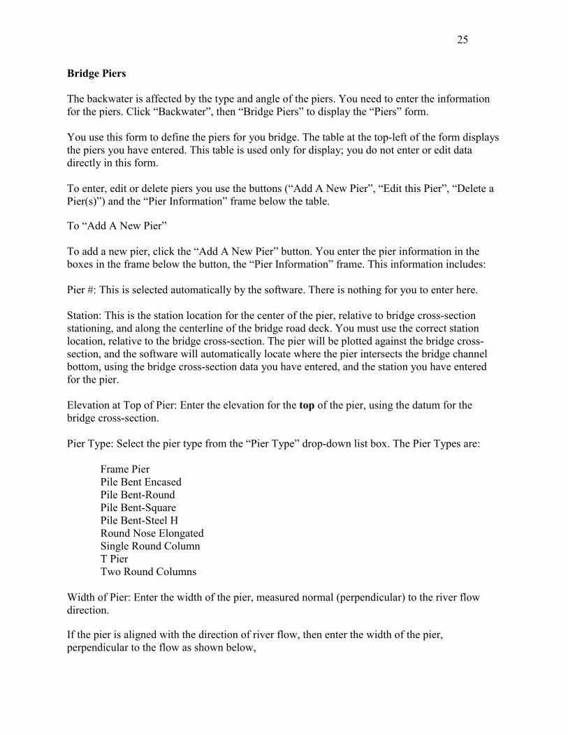
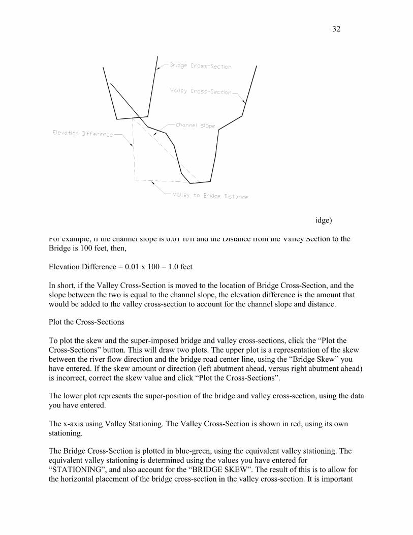
Width of Pier: Enter the width of the pier, measured normal (perpendicular) to the river flow direction. If the pier is aligned with the direction of river flow, then enter the width of the pier, perpendicular to the flow as shown below,

26

River Flow Direction

Pier Width

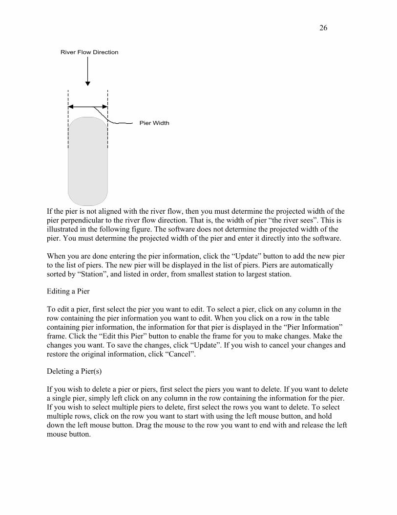
If the pier is not aligned with the river flow, then you must determine the projected width of the pier perpendicular to the river flow direction. That is, the width of pier “the river sees”. This is illustrated in the following figure. The software does not determine the projected width of the pier. You must determine the projected width of the pier and enter it directly into the software. When you are done entering the pier information, click the “Update” button to add the new pier to the list of piers. The new pier will be displayed in the list of piers. Piers are automatically sorted by “Station”, and listed in order, from smallest station to largest station. Editing a Pier To edit a pier, first select the pier you want to edit. To select a pier, click on any column in the row containing the pier information you want to edit. When you click on a row in the table containing pier information, the information for that pier is displayed in the “Pier Information” frame. Click the “Edit this Pier” button to enable the frame for you to make changes. Make the changes you want. To save the changes, click “Update”. If you wish to cancel your changes and restore the original information, click “Cancel”. Deleting a Pier(s) If you wish to delete a pier or piers, first select the piers you want to delete. If you want to delete a single pier, simply left click on any column in the row containing the information for the pier. If you wish to select multiple piers to delete, first select the rows you want to delete. To select multiple rows, click on the row you want to start with using the left mouse button, and hold down the left mouse button. Drag the mouse to the row you want to end with and release the left mouse button.

27

River Flow Direction

Pier Width

After selecting the row or rows for the piers you want to delete, click the “Delete a Pier(s)” button. A message box will show the pier #’s you have selected for deletion, and confirm you want to delete. Plotting the Piers To plot the Bridge Cross-Section with the Piers, click the “Plot the Cross-Section” button. You need have previously entered the bridge cross-section information. The piers are plotted at the station location you have entered. The software determines where the piers intersect the bridge channel bottom by interpolating the pier station against the bridge cross-section. The width of the pier is shown to scale, using the horizontal scaling shown at the bottom of the plot. To send a copy of the plot to your printer, click “Print the Plot”. Printing the Data To print a copy of the pier data, in tabular form, click “Print the Data”.

28

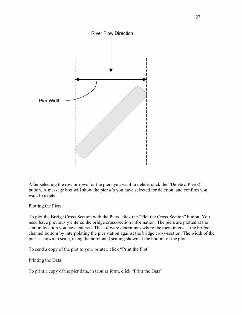
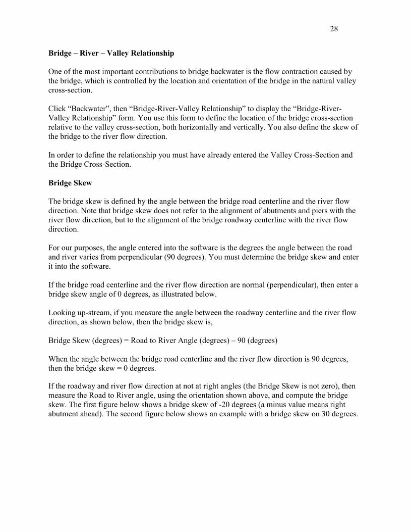
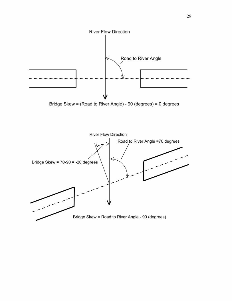
Bridge – River – Valley Relationship One of the most important contributions to bridge backwater is the flow contraction caused by the bridge, which is controlled by the location and orientation of the bridge in the natural valley cross-section. Click “Backwater”, then “Bridge-River-Valley Relationship” to display the “Bridge-River-Valley Relationship” form. You use this form to define the location of the bridge cross-section relative to the valley cross-section, both horizontally and vertically. You also define the skew of the bridge to the river flow direction. In order to define the relationship you must have already entered the Valley Cross-Section and the Bridge Cross-Section. Bridge Skew The bridge skew is defined by the angle between the bridge road centerline and the river flow direction. Note that bridge skew does not refer to the alignment of abutments and piers with the river flow direction, but to the alignment of the bridge roadway centerline with the river flow direction. For our purposes, the angle entered into the software is the degrees the angle between the road and river varies from perpendicular (90 degrees). You must determine the bridge skew and enter it into the software. If the bridge road centerline and the river flow direction are normal (perpendicular), then enter a bridge skew angle of 0 degrees, as illustrated below. Looking up-stream, if you measure the angle between the roadway centerline and the river flow direction, as shown below, then the bridge skew is, Bridge Skew (degrees) = Road to River Angle (degrees) – 90 (degrees) When the angle between the bridge road centerline and the river flow direction is 90 degrees, then the bridge skew = 0 degrees. If the roadway and river flow direction at not at right angles (the Bridge Skew is not zero), then measure the Road to River angle, using the orientation shown above, and compute the bridge skew. The first figure below shows a bridge skew of -20 degrees (a minus value means right abutment ahead). The second figure below shows an example with a bridge skew on 30 degrees.

29

River Flow Direction

Road to River Angle

Bridge Skew = (Road to River Angle) - 90 (degrees) = 0 degrees

River Flow DirectionRoad to River Angle =70 degrees

Bridge Skew = 70-90 = -20 degrees

Bridge Skew = Road to River Angle - 90 (degrees)

30

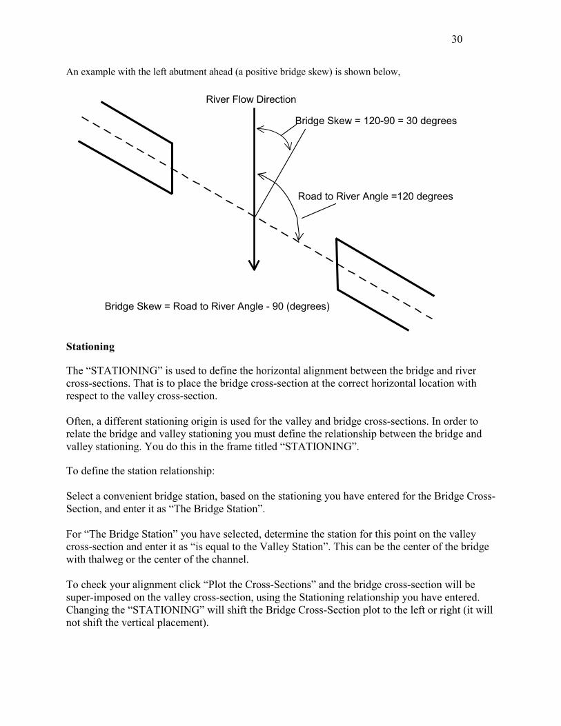
An example with the left abutment ahead (a positive bridge skew) is shown below,

River Flow Direction

Road to River Angle =120 degrees

Bridge Skew = Road to River Angle - 90 (degrees)

Bridge Skew = 120-90 = 30 degrees

Stationing The “STATIONING” is used to define the horizontal alignment between the bridge and river cross-sections. That is to place the bridge cross-section at the correct horizontal location with respect to the valley cross-section. Often, a different stationing origin is used for the valley and bridge cross-sections. In order to relate the bridge and valley stationing you must define the relationship between the bridge and valley stationing. You do this in the frame titled “STATIONING”. To define the station relationship: Select a convenient bridge station, based on the stationing you have entered for the Bridge Cross-Section, and enter it as “The Bridge Station”. For “The Bridge Station” you have selected, determine the station for this point on the valley cross-section and enter it as “is equal to the Valley Station”. This can be the center of the bridge with thalweg or the center of the channel. To check your alignment click “Plot the Cross-Sections” and the bridge cross-section will be super-imposed on the valley cross-section, using the Stationing relationship you have entered. Changing the “STATIONING” will shift the Bridge Cross-Section plot to the left or right (it will not shift the vertical placement).

31

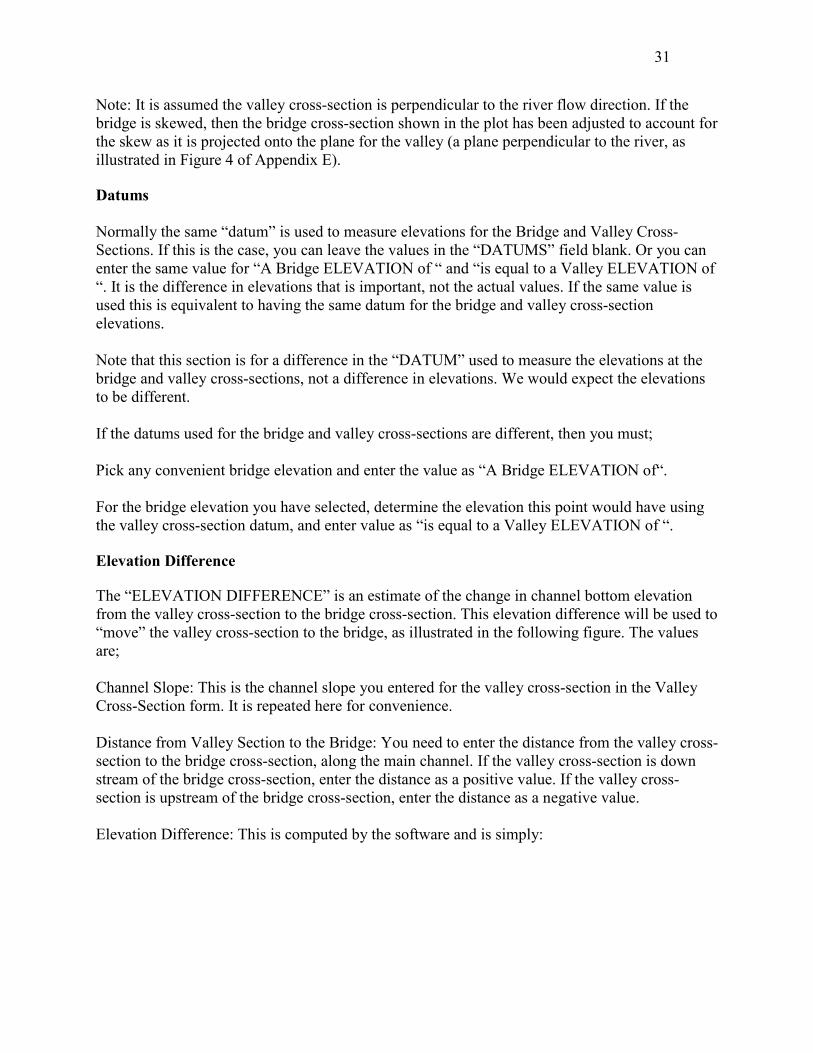
Note: It is assumed the valley cross-section is perpendicular to the river flow direction. If the bridge is skewed, then the bridge cross-section shown in the plot has been adjusted to account for the skew as it is projected onto the plane for the valley (a plane perpendicular to the river, as illustrated in Figure 4 of Appendix E). Datums Normally the same “datum” is used to measure elevations for the Bridge and Valley Cross-Sections. If this is the case, you can leave the values in the “DATUMS” field blank. Or you can enter the same value for “A Bridge ELEVATION of “ and “is equal to a Valley ELEVATION of “. It is the difference in elevations that is important, not the actual values. If the same value is used this is equivalent to having the same datum for the bridge and valley cross-section elevations. Note that this section is for a difference in the “DATUM” used to measure the elevations at the bridge and valley cross-sections, not a difference in elevations. We would expect the elevations to be different. If the datums used for the bridge and valley cross-sections are different, then you must; Pick any convenient bridge elevation and enter the value as “A Bridge ELEVATION of“. For the bridge elevation you have selected, determine the elevation this point would have using the valley cross-section datum, and enter value as “is equal to a Valley ELEVATION of “. Elevation Difference The “ELEVATION DIFFERENCE” is an estimate of the change in channel bottom elevation from the valley cross-section to the bridge cross-section. This elevation difference will be used to “move” the valley cross-section to the bridge, as illustrated in the following figure. The values are; Channel Slope: This is the channel slope you entered for the valley cross-section in the Valley Cross-Section form. It is repeated here for convenience. Distance from Valley Section to the Bridge: You need to enter the distance from the valley cross-section to the bridge cross-section, along the main channel. If the valley cross-section is down stream of the bridge cross-section, enter the distance as a positive value. If the valley cross-section is upstream of the bridge cross-section, enter the distance as a negative value. Elevation Difference: This is computed by the software and is simply:

32

Elevation Difference = (Channel Slope) x (Distance from Valley Section to the Bridge) For example, if the channel slope is 0.01 ft/ft and the Distance from the Valley Section to the Bridge is 100 feet, then, Elevation Difference = 0.01 x 100 = 1.0 feet In short, if the Valley Cross-Section is moved to the location of Bridge Cross-Section, and the slope between the two is equal to the channel slope, the elevation difference is the amount that would be added to the valley cross-section to account for the channel slope and distance. Plot the Cross-Sections To plot the skew and the super-imposed bridge and valley cross-sections, click the “Plot the Cross-Sections” button. This will draw two plots. The upper plot is a representation of the skew between the river flow direction and the bridge road center line, using the “Bridge Skew” you have entered. If the skew amount or direction (left abutment ahead, versus right abutment ahead) is incorrect, correct the skew value and click “Plot the Cross-Sections”. The lower plot represents the super-position of the bridge and valley cross-section, using the data you have entered. The x-axis using Valley Stationing. The Valley Cross-Section is shown in red, using its own stationing. The Bridge Cross-Section is plotted in blue-green, using the equivalent valley stationing. The equivalent valley stationing is determined using the values you have entered for “STATIONING”, and also account for the “BRIDGE SKEW”. The result of this is to allow for the horizontal placement of the bridge cross-section in the valley cross-section. It is important

33

that this horizontal alignment is correct. The horizontal alignment has a large impact on the backwater calculations, and the horizontal placement of the bridge in the valley cross-section must be a reasonable approximation for your site conditions. The horizontal placement affects the computation of the flow distribution upstream of the bridge, as illustrated as Qa, Qb and Qb in Figures 1 and 2 in Appendix E. In turn, the values of Qa, Qb and Qc affect the amount of backwater. The y-axis uses the “Elevation at the Bridge”. The bridge cross-section is plotted using the elevations you have entered for the bridge cross-section. The valley elevations are plotted as if the valley “has been moved” to the bridge. That is, the computed “Elevation Difference” has been added to the valley elevations and these adjusted valley elevations values are plotted to present the valley elevations at the bridge, if the valley is moved to the bridge, using the channel slope and distance from the valley to the bridge. If the computed “Elevation Difference” is equal to the elevation difference between the lowest elevations in the valley and bridge cross-section then the valley and channel bottoms will have the same elevation on this plot. In practice, this is seldom the case. Often the bridge cross-section is taken at an existing bridge and the channel bottom has been reshaped by flow or man, and no longer presents the natural channel conditions. It may be that the valley cross-section is also not typical, and needs to be edited. Also, the channel slope estimated for the river in the vicinity of the bridge may not be representative of the channel slope between the bridge and valley cross-section. You can expect the bridge channel bottom and valley channel bottom not to line up exactly (vertically), but should be concerned if the difference is large. If, after moving the valley to the bridge the lowest bridge channel elevation and adjusted lowest valley channel elevation differs by more than 1 foot, you are alerted to this by a message box. If you get this message, you may want to review you valley cross-section data and bridge cross-section data to ensure they are reasonable. Printing the Data and Plots To print a copy of the data you have used to define the bridge – valley –river relationship, click the “Print the Data” button at the top-left of the form. This will also print copy of the bridge-river skew plot. To print a copy of the super-imposed bridge-valley plot, click the “Print the Plot” button.

34

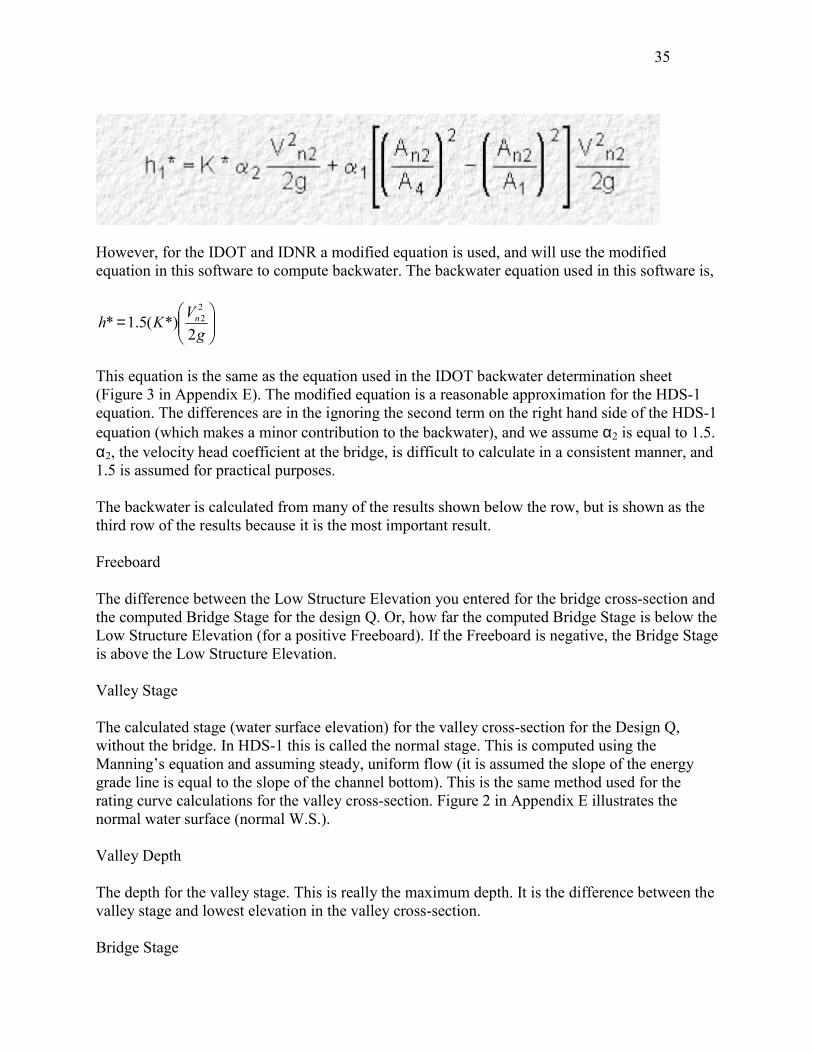
Compute Backwater (Without Roadway Overtopping) Click “Backwater”, followed by “Compute Backwater (Without Roadway Overtopping)” to display the “Bridge Backwater – No Overtopping” form. You use this form to compute the Bridge Backwater. Roadway overtopping is not considered. For many sites, this may be sufficient. The methodology for computing backwater is essentially the same methodology that is used by the IDOT for doing hand calculations. An example of calculation worksheet is shown as Figure 3 in Appendix E. In order to compute the backwater you need to have entered: The Valley Cross-Section The Bridge Cross-Section The Piers The Bridge-River-Valley Relationship Design Q’s Enter the Design Q’s in the upper-left table. The backwater will be computed for each Design Q value in the table. You can type the Q values directly into table. You can also copy Q values from other locations and paste them into the table. For example, you could copy selected values from the USGS – Eash or USGS – Lara form and paste them into the table. See appendix A for more information on copying and pasting. Compute Backwater To compute the backwater results click the “Compute Backwater” button. The backwater will be computed for each Design Q in the table and the results displayed in the table beneath the “Compute Backwater” button. The results are displayed in columns. There will one column for each design Q. The results displayed in the table for each Q, starting with the top row are: Return Period This is simply a copy of the value you entered for the return period in the Design Q’s table. Design Q A copy of the value you entered into the Design Q table, rounded to the nearest integer value. (If example, if you entered 10,000.99 this would be shown as 10,001). The results in the column are the results for this Design Q. Backwater: h* The calculated bridge backwater for the Design Q. In HDS-1 backwater is calculated from

35

However, for the IDOT and IDNR a modified equation is used, and will use the modified equation in this software to compute backwater. The backwater equation used in this software is,

���

����

�=

gVKh n

2*)(5.1*

22

This equation is the same as the equation used in the IDOT backwater determination sheet (Figure 3 in Appendix E). The modified equation is a reasonable approximation for the HDS-1 equation. The differences are in the ignoring the second term on the right hand side of the HDS-1 equation (which makes a minor contribution to the backwater), and we assume α2 is equal to 1.5. α2, the velocity head coefficient at the bridge, is difficult to calculate in a consistent manner, and 1.5 is assumed for practical purposes. The backwater is calculated from many of the results shown below the row, but is shown as the third row of the results because it is the most important result. Freeboard The difference between the Low Structure Elevation you entered for the bridge cross-section and the computed Bridge Stage for the design Q. Or, how far the computed Bridge Stage is below the Low Structure Elevation (for a positive Freeboard). If the Freeboard is negative, the Bridge Stage is above the Low Structure Elevation. Valley Stage The calculated stage (water surface elevation) for the valley cross-section for the Design Q, without the bridge. In HDS-1 this is called the normal stage. This is computed using the Manning’s equation and assuming steady, uniform flow (it is assumed the slope of the energy grade line is equal to the slope of the channel bottom). This is the same method used for the rating curve calculations for the valley cross-section. Figure 2 in Appendix E illustrates the normal water surface (normal W.S.). Valley Depth The depth for the valley stage. This is really the maximum depth. It is the difference between the valley stage and lowest elevation in the valley cross-section. Bridge Stage

36

The maximum depth at the valley and bridge is assumed to be the same. That is the depth of water at the bridge is assumed to be the same as the normal valley water surface without the bridge. If you examine Figure 2 in Appendix E you can see that the stage at the bridge (at Sect. 2) is approximately equal to normal stage (the stage without the bridge). Of course, because of the bridge a backwater is created upstream of the bridge to generate sufficient energy to force the design Q through the reduced flow area created by the bridge. To get the bridge stage the valley depth is added to the lowest elevation in the bridge cross-section. In HDS-1, the stage at the bridge is equal to the natural stage at the bridge (the stage without the bridge). An2 The gross cross-sectional area (including the area occupied by the piers) of flow in the bridge cross-section at the bridge stage. Section C in Figure 2 in Appendix E provides an illustration. Projected An2 If the bridge is skewed from the perpendicular this is the area of flow projected onto the plane perpendicular to the river flow direction. This is the water flow area that “the river sees” at the bridge. If the bridge skew is 0, then the Projected An2 is equal to An2. If the bridge is skewed then the Projected An2 will be less than An2. Figure 4 in Appendix E illustrates the projection of the bridge opening on a plane perpendicular to the river cross-section. Vn2 The average velocity in the bridge cross-section.

2Pr2

AnojectedQDesignVn =

b-width estimation (this heading is not a row in the table) The b-width is an estimate of the effective width of the bridge opening for the purpose of passing the design flow, as illustrated in Figures 1 and 2 in Appendix E. For vertical wingwalls the b-width is simply the distance between the wingwalls. For spillthrough abutments the b-width must be estimated to account for the fact that the flow area above the spillthrough abutments does not convey the full depth of flow. The flowing items are used to estimate the b-width. Bridge b-Width Elev. The bridge b-width elevation. The “b” points are used to determine the distribution of flow upstream of the bridge. That is, the distribution of upstream flow between the main channel (the bridge opening) and left and right of the effective bridge opening. The bridge b-width elevation is assumed to be equal to 2/3 of the depth water at the bridge. This is illustrated in the following figure.

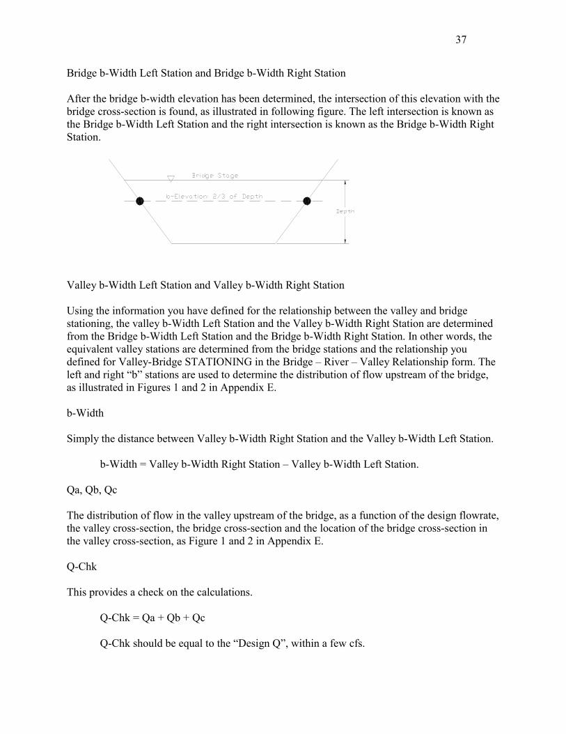
37

Bridge b-Width Left Station and Bridge b-Width Right Station After the bridge b-width elevation has been determined, the intersection of this elevation with the bridge cross-section is found, as illustrated in following figure. The left intersection is known as the Bridge b-Width Left Station and the right intersection is known as the Bridge b-Width Right Station.

Valley b-Width Left Station and Valley b-Width Right Station Using the information you have defined for the relationship between the valley and bridge stationing, the valley b-Width Left Station and the Valley b-Width Right Station are determined from the Bridge b-Width Left Station and the Bridge b-Width Right Station. In other words, the equivalent valley stations are determined from the bridge stations and the relationship you defined for Valley-Bridge STATIONING in the Bridge – River – Valley Relationship form. The left and right “b” stations are used to determine the distribution of flow upstream of the bridge, as illustrated in Figures 1 and 2 in Appendix E. b-Width Simply the distance between Valley b-Width Right Station and the Valley b-Width Left Station. b-Width = Valley b-Width Right Station – Valley b-Width Left Station. Qa, Qb, Qc The distribution of flow in the valley upstream of the bridge, as a function of the design flowrate, the valley cross-section, the bridge cross-section and the location of the bridge cross-section in the valley cross-section, as Figure 1 and 2 in Appendix E. Q-Chk This provides a check on the calculations. Q-Chk = Qa + Qb + Qc

Q-Chk should be equal to the “Design Q”, within a few cfs.

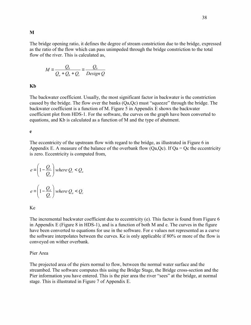
38

M The bridge opening ratio, it defines the degree of stream constriction due to the bridge, expressed as the ratio of the flow which can pass unimpeded through the bridge constriction to the total flow of the river. This is calculated as,

QDesignQ

QQQQM b

cba

b =++

=

Kb The backwater coefficient. Usually, the most significant factor in backwater is the constriction caused by the bridge. The flow over the banks (Qa,Qc) must “squeeze” through the bridge. The backwater coefficient is a function of M. Figure 5 in Appendix E shows the backwater coefficient plot from HDS-1. For the software, the curves on the graph have been converted to equations, and Kb is calculated as a function of M and the type of abutment. e The eccentricity of the upstream flow with regard to the bridge, as illustrated in Figure 6 in Appendix E. A measure of the balance of the overbank flow (Qa,Qc). If Qa = Qc the eccentricity is zero. Eccentricity is computed from,

aca

c QQwhereQQe <��

�

����

�−= 1

cac

a QQwhereQQe <��

�

����

�−= 1

Ke The incremental backwater coefficient due to eccentricity (e). This factor is found from Figure 6 in Appendix E (Figure 8 in HDS-1), and is a function of both M and e. The curves in the figure have been converted to equations for use in the software. For e values not represented as a curve the software interpolates between the curves. Ke is only applicable if 80% or more of the flow is conveyed on wither overbank. Pier Area The projected area of the piers normal to flow, between the normal water surface and the streambed. The software computes this using the Bridge Stage, the Bridge cross-section and the Pier information you have entered. This is the pier area the river “sees” at the bridge, at normal stage. This is illustrated in Figure 7 of Appendix E.

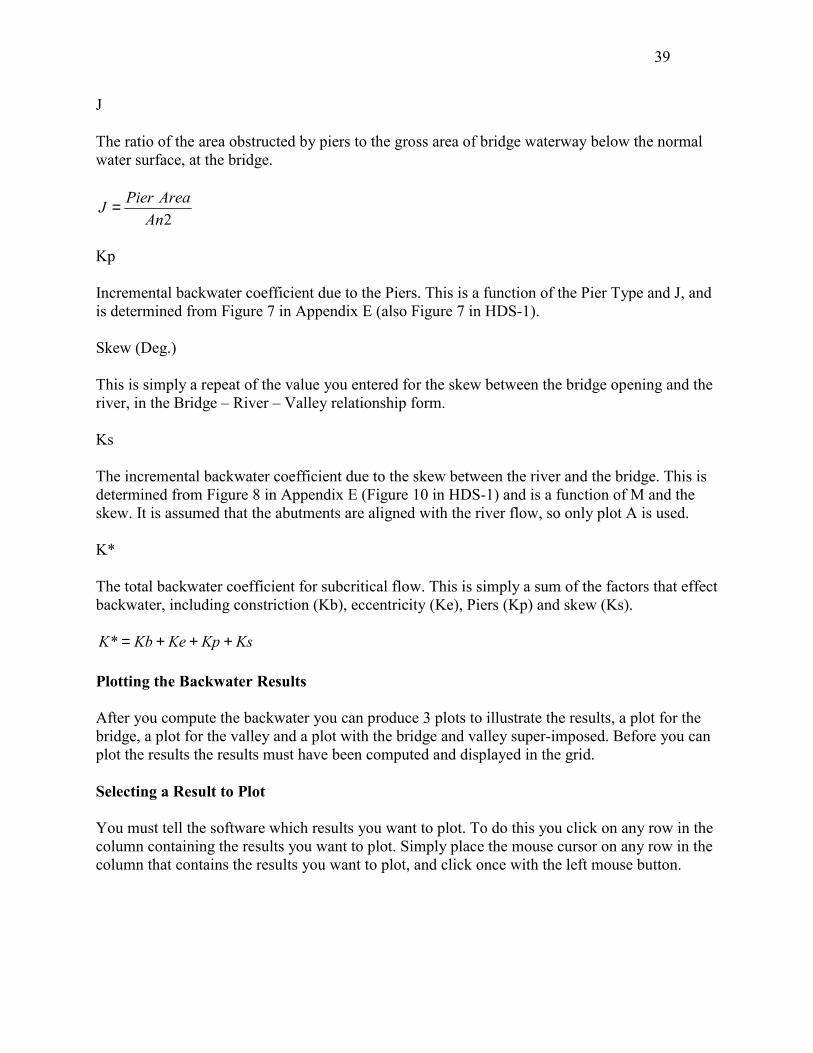
39

J The ratio of the area obstructed by piers to the gross area of bridge waterway below the normal water surface, at the bridge.

2AnAreaPierJ =

Kp Incremental backwater coefficient due to the Piers. This is a function of the Pier Type and J, and is determined from Figure 7 in Appendix E (also Figure 7 in HDS-1). Skew (Deg.) This is simply a repeat of the value you entered for the skew between the bridge opening and the river, in the Bridge – River – Valley relationship form. Ks The incremental backwater coefficient due to the skew between the river and the bridge. This is determined from Figure 8 in Appendix E (Figure 10 in HDS-1) and is a function of M and the skew. It is assumed that the abutments are aligned with the river flow, so only plot A is used. K* The total backwater coefficient for subcritical flow. This is simply a sum of the factors that effect backwater, including constriction (Kb), eccentricity (Ke), Piers (Kp) and skew (Ks).

KsKpKeKbK +++=* Plotting the Backwater Results After you compute the backwater you can produce 3 plots to illustrate the results, a plot for the bridge, a plot for the valley and a plot with the bridge and valley super-imposed. Before you can plot the results the results must have been computed and displayed in the grid. Selecting a Result to Plot You must tell the software which results you want to plot. To do this you click on any row in the column containing the results you want to plot. Simply place the mouse cursor on any row in the column that contains the results you want to plot, and click once with the left mouse button.

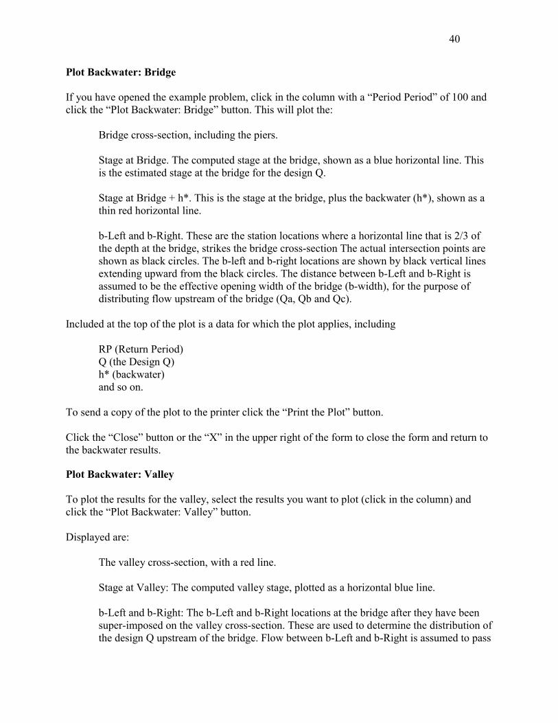
40

Plot Backwater: Bridge If you have opened the example problem, click in the column with a “Period Period” of 100 and click the “Plot Backwater: Bridge” button. This will plot the:

Bridge cross-section, including the piers. Stage at Bridge. The computed stage at the bridge, shown as a blue horizontal line. This is the estimated stage at the bridge for the design Q. Stage at Bridge + h*. This is the stage at the bridge, plus the backwater (h*), shown as a thin red horizontal line. b-Left and b-Right. These are the station locations where a horizontal line that is 2/3 of the depth at the bridge, strikes the bridge cross-section The actual intersection points are shown as black circles. The b-left and b-right locations are shown by black vertical lines extending upward from the black circles. The distance between b-Left and b-Right is assumed to be the effective opening width of the bridge (b-width), for the purpose of distributing flow upstream of the bridge (Qa, Qb and Qc).

Included at the top of the plot is a data for which the plot applies, including

RP (Return Period) Q (the Design Q) h* (backwater) and so on.

To send a copy of the plot to the printer click the “Print the Plot” button. Click the “Close” button or the “X” in the upper right of the form to close the form and return to the backwater results. Plot Backwater: Valley To plot the results for the valley, select the results you want to plot (click in the column) and click the “Plot Backwater: Valley” button. Displayed are: The valley cross-section, with a red line. Stage at Valley: The computed valley stage, plotted as a horizontal blue line.

b-Left and b-Right: The b-Left and b-Right locations at the bridge after they have been super-imposed on the valley cross-section. These are used to determine the distribution of the design Q upstream of the bridge. Flow between b-Left and b-Right is assumed to pass

41

directly through the bridge opening. Flow to the left of b-Left and the right of b-Right must be diverted in order to pass through the bridge opening. Qa: The portion of the design Q to the left of b-Left. This is the valley flow left of the bridge opening which must contract in order to pass through the bridge opening. Qb: The portion of the design Q between b-Left and b-Right. This is considered main channel flow and will pass directly through the effective bridge opening without having to contract. Qc: The portion of the design Q to the right of b-Right. This is the valley flow to the right of the effective bridge opening which must contract in order to pass through the bridge opening.

Plot Backwater: Bridge and Valley To plot the results with the Bridge and Valley super-imposed, click the “Plot Backwater: Bridge and Valley” button to display the “Backwater: Bridge – Valley Plot” form. This plot can be busy because it shows all the essential elements of the computed results. The Bridge Cross-Section (blue-green) is shown super-imposed with the valley cross-section (red). This is the relationship as shown in the plot for the Bridge – River – Valley relationship. Valley stationing is used for the x-axis, and bridge elevation for the y-axis. For plotting elevation the valley has been “moved” to the bridge, using the channel slope and distance entered for the Bridge – River – Valley relationship. The Bridge Stage is shown as the thicker blue horizontal line. The Bridge Stage + h* (backwater) is shown as the horizontal red line. The normal stage at the valley, translated to the bridge, is shown as the thin blue horizontal line, with the title “Valley Stage at Bridge” shown just below the line. If, after translation, the lowest elevation of the Bridge Cross-Section and Valley Cross-Section were equal, then the “Valley Stage at Bridge” and “Bridge Stage” would have the same elevation. As discussed in section x, the Bridge – River – Valley Relationship section, these are unlikely to match exactly and the plot gives some idea of the difference. For the purposes of computation the depth at the bridge is assumed to be the same as the depth of the normal valley stage. Backwater with Roadway Overtopping You may compute the backwater for the case where there could be road grade overflow. With road grade overflow if the backwater elevation exceeds the lowest elevation of the road grade the design discharge is balanced between flow through the bridge and flow overtopping the road grade. If the road grade is not overtopped, then the backwater results will be the same as the no road grade overtopping since the entire design Q passes though the bridge.

42

Road Grade Profile (For Overtopping) To enter a road profile to check for overtopping click “Backwater”, followed by “Road Grade Profile (For Overtopping)” to display the “Road Grade Profile for Overflow” form. You enter the road profile as a series of Station and Elevation points. Note that the road profile is not necessarily the profile for the bridge. The road profile you should enter is the profile for the first location that would be overtopped by the backwater. This would often be one of the bridge approaches. Enter the stage and elevation data that describes the profile. The roadway is assumed straight line between points, so enter as many points as you feel are necessarily to capture the vertical curvature of the road. To plot the profile, click the “Plot the Profile” button. Keep in mind the profile will have a vertical exaggeration. To print a copy of the profile, click the “Print the Profile” button. Compute Backwater (With Roadway Overtopping) To compute the backwater with consideration of roadway overtopping, click “Backwater”, then “Compute Backwater (With Roadway Overtopping)” to display the “Bridge Backwater – With Roadway Overtopping” form. Backwater is computed here with consider of possible overtopping of the road grade profile that has been entered. You first need to enter the Design Q’s. You may copy these values from the Backwater without Overtopping form and paste the values into this form, or enter the values directly. See appendix A for more information on copying and pasting. After entering the Design Q’s, click the “Compute Backwater (With Overtopping)” button to compute the backwater with consideration of overtopping. How It Works The software distributes the design Q as flow through the bridge and flow overtopping the road grade profile. First, it is assumed the entire design Q passes through the Bridge and the backwater is computed. Then the elevation of the Bridge Stage + h* (backwater) is compared to the lowest elevation of the Road Grade Profile you have entered. If elevation does not exceed the lowest road grade elevation, then no overtopping will take place and the solution is displayed (which will the same as the solution without overtopping since no overtopping takes place). If the Bridge Stage + h* elevation is greater than the lowest elevation then overtopping will take place, and the overtopping Q is computed, treating the roadway as a broad crested weir (See appendix D for more information on overtopping computations). However, with flow overtopping the road grade, the Q that passes through the Bridge will be reduced, reducing the backwater, which will reduce the overtopping, etc. The software iterates until convergence is reached: the Q passing through the bridge (called the Q-Bridge) plus the Q overtopping the road (due to the backwater from the Bridge Q) is equal to the design Q.

43

The description of many of the items shown in the results grid are the same as the grid without overtopping (although the values may be different). We will only discuss the differences in the results tables for overtopping and no overtopping. Q-Overtop This is the Q overtopping the road, at the Overtop Stage. This is computed treating the road profile as a broad crested weir. If Q-Overtop is “0”, this means no overtopping occurred at the Design Q. The Q that overtops the road grade is assumed to not pass through the bridge opening. Overtop Stage This is the stage at the roadway. The stage at the roadway is assumed to be equal to the bridge stage plus the backwater increment. Hence, Overtop Stage = Bridge Stage + h* Maximum Overtop Depth The maximum depth of flow at the roadway. This is simply the overtop stage minus the lowest elevation of the roadway profile. If the Overtop Stage is less than or equal the lowest elevation of the roadway profile, this value is shown as “0.00”. This means there was no overtopping for the Design Q, and Q-Overtop will be “0”. Q-Bridge The portion of the design Q passing through the bridge. Design Q = Q-Bridge + Q-Overtop Or Q-Bridge = (Design Q) – (Q-Overtop) The remainder of the results grid is the same as the backwater grid without overtopping, except the results are for Q-Bridge; that is the backwater computations are for the flow passing through the bridge. At convergence, Q-Overtop is going over the roadway and Q-Bridge is passing though the bridge. It is assumed the flow overtopping the road grade will not pass through the bridge. All the backwater computations in this form are made using Q-Bridge as the flowrate. In fact, if you go to the backwater form without overtopping and enter Q-Bridge as a Design Q, you will get the same backwater results as for Bridge Backwater with overtopping. If there is overtopping, this will reduce the backwater due to the bridge (without overtopping) since Q-Bridge will be less than the Design Q. Plotting The Results

44

The first 3 plots have the same format as for backwater without overtopping, except that the results are for the flowrate that passes through the Bridge, Q-Bridge. An additional plot for overtopping has been added. Click on the column with the results you want to plot, and click the “Plot Road Grade Overflow” button to display the “Road Grade Overflow Plot” form. This form shows the road grade profile, and the stage at the road grade as a blue horizontal line with the title “Overflow Stage (Bridge Stage + h*)”. This stage results in the “Q-Overflow” value shown at the top of the plot. If there is no overflow, the blue line will be shown on the x-axis and “Q-Overflow” will be equal to 0. This completes the user manual. References Eash-2001: Eash, David A., Techniques for estimating flood-frequency discharges for streams in Iowa. U.S. Geological Survey, Water-Resources Investigation Report 00-4233, Iowa Department of Transportation and the Iowa Highway Research Board (Project HR-395A), Iowa City, Iowa 2001. Eash-2003: Eash, David A., Main-Channel Slopes of Selected Streams in Iowa for Estimation of Flood-Frequency Discharges. U.S. Geological Survey, Water-Resources Investigation Report 03-4120, Iowa Department of Transportation and the Iowa Highway Research Board (Project HR-456), Iowa City, Iowa 2003. HDS-1: Hydraulic Design Series No. 1, Hydraulics of Bridge Waterways, U.S. Department of Transportation, Federal Highway Administration, Bureau of Public Roads, Washington, D.C., 1970. Revised 1978 Edition with Errata Sheet. Lara-1987: Lara, Oscar G., Method for estimating the magnitude and frequency of floods at ungaged sites on unregulated rural streams in Iowa. U.S. Geological Survey, Water-Resources Investigation Report 87-4132, Iowa Department of Transportation, Highway Division, Highway Research Board, Iowa City, Iowa, 1987.

45

Appendix A: Copying and Pasting Values You may often find it convenient to copy and paste values from one grid to another. For example, you may want to copy the design Q values you have generated into the rating curve or backwater grid. To Copy: First, select the values you want to copy. Click on a cell, click and hold down the left mouse button, move the mouse over the area you want to copy, then release the mouse button. Press Ctrl-C (this means press and down the Ctrl key, then press the C key, then release both) to copy the selection to the clip board. To Paste: Go to the grid where you wish to paste the copied data. Select the area to paste to. To select an area, click the cell at the upper left of the area you want to copy to, click and hold down the left mouse button, move the mouse over the area you want to paste to, then release the left mouse button. Press Ctr-V (this means press and down the Ctrl key, then press the this means press and down the Ctrl key, then press the V key, then release both) to paste the data from the clipboard to the selected area.

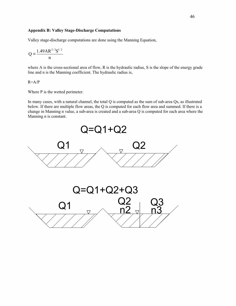
46

Appendix B: Valley Stage-Discharge Computations Valley stage-discharge computations are done using the Manning Equation,

nSAR49.1Q

2/13/2

=

where A is the cross-sectional area of flow, R is the hydraulic radius, S is the slope of the energy grade line and n is the Manning coefficient. The hydraulic radius is, R=A/P Where P is the wetted perimeter. In many cases, with a natural channel, the total Q is computed as the sum of sub-area Qs, as illustrated below. If there are multiple flow areas, the Q is computed for each flow area and summed. If there is a change in Manning n value, a sub-area is created and a sub-area Q is computed for each area where the Manning n is constant.

Q=Q1+Q2

Q1 Q2

Q=Q1+Q2+Q3Q2n2

Q3n3Q1

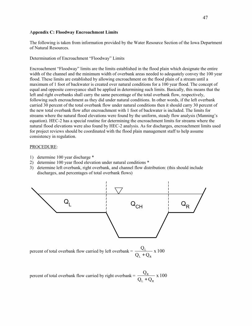
47

Appendix C: Floodway Encroachment Limits The following is taken from information provided by the Water Resource Section of the Iowa Department of Natural Resources. Determination of Encroachment “Floodway” Limits Encroachment “Floodway” limits are the limits established in the flood plain which designate the entire width of the channel and the minimum width of overbank areas needed to adequately convey the 100 year flood. These limits are established by allowing encroachment on the flood plain of a stream until a maximum of 1 foot of backwater is created over natural conditions for a 100 year flood. The concept of equal and opposite conveyance shall be applied in determining such limits. Basically, this means that the left and right overbanks shall carry the same percentage of the total overbank flow, respectively, following such encroachment as they did under natural conditions. In other words, if the left overbank carried 30 percent of the total overbank flow under natural conditions then it should carry 30 percent of the new total overbank flow after encroachment with 1 foot of backwater is included. The limits for streams where the natural flood elevations were found by the uniform, steady flow analysis (Manning’s equation). HEC-2 has a special routine for determining the encroachment limits for streams where the natural flood elevations were also found by HEC-2 analysis. As for discharges, encroachment limits used for project reviews should be coordinated with the flood plain management staff to help assume consistency in regulation. PROCEDURE: 1) determine 100 year discharge * 2) determine 100 year flood elevation under natural conditions * 3) determine left overbank, right overbank, and channel flow distribution: (this should include

discharges, and percentages of total overbank flows)

Q Q QL CH R

percent of total overbank flow carried by left overbank = 100xQQ

Q

RL

L

+

percent of total overbank flow carried by right overbank = 100xQQ

Q

RL

R

+

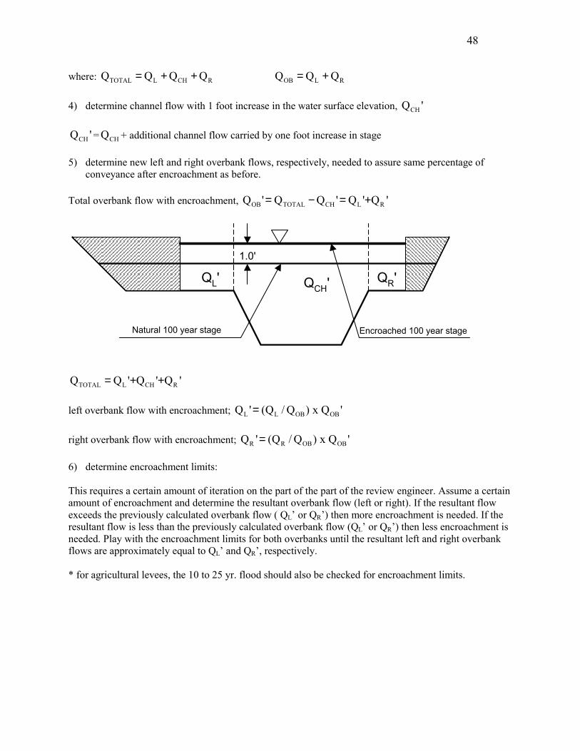
48

where: RCHLTOTAL QQQQ ++= RLOB QQQ += 4) determine channel flow with 1 foot increase in the water surface elevation, 'QCH

'QCH = CHQ + additional channel flow carried by one foot increase in stage 5) determine new left and right overbank flows, respectively, needed to assure same percentage of

conveyance after encroachment as before. Total overbank flow with encroachment, 'Q'Q'QQ' RLCHTOTALOB +=−=Q

QL' QCH' QR'1.0'

Natural 100 year stage Encroached 100 year stage

'Q'Q'QQ RCHLTOTAL ++= left overbank flow with encroachment; 'Qx)Q/Q('Q OBOBLL = right overbank flow with encroachment; 'Qx)Q/Q('Q OBOBRR = 6) determine encroachment limits: This requires a certain amount of iteration on the part of the part of the review engineer. Assume a certain amount of encroachment and determine the resultant overbank flow (left or right). If the resultant flow exceeds the previously calculated overbank flow ( QL’ or QR’) then more encroachment is needed. If the resultant flow is less than the previously calculated overbank flow (QL’ or QR’) then less encroachment is needed. Play with the encroachment limits for both overbanks until the resultant left and right overbank flows are approximately equal to QL’ and QR’, respectively. * for agricultural levees, the 10 to 25 yr. flood should also be checked for encroachment limits.

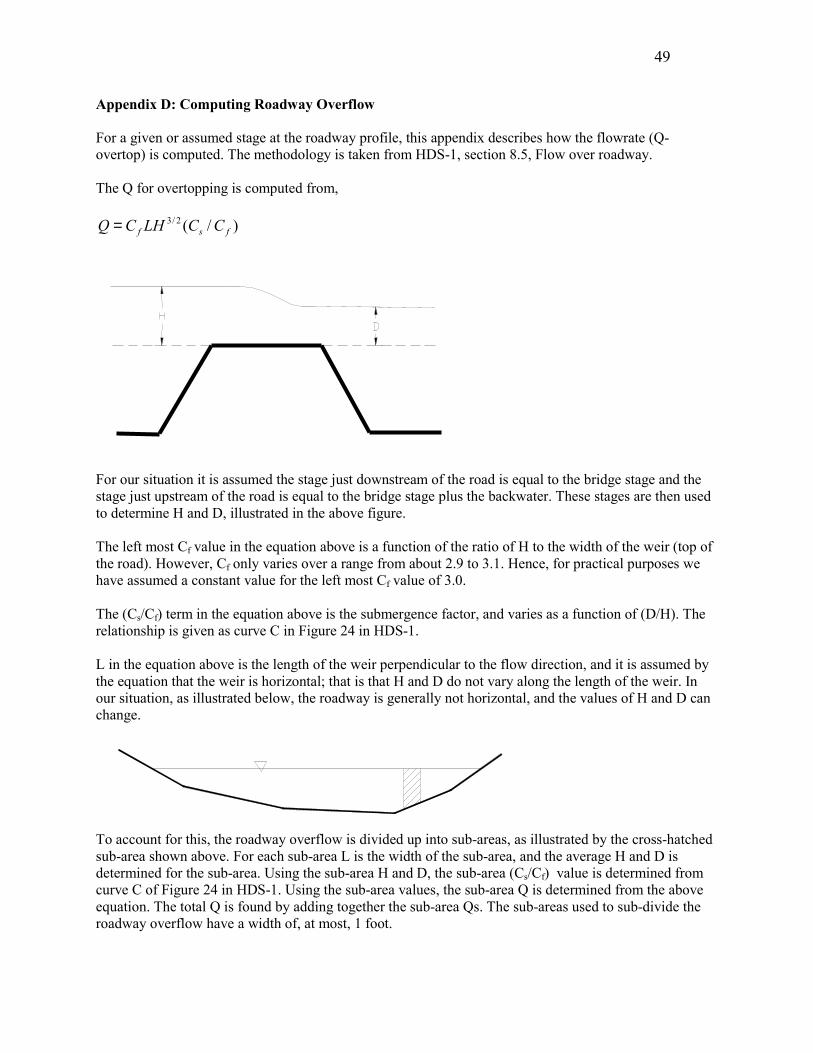
49

Appendix D: Computing Roadway Overflow For a given or assumed stage at the roadway profile, this appendix describes how the flowrate (Q-overtop) is computed. The methodology is taken from HDS-1, section 8.5, Flow over roadway. The Q for overtopping is computed from,

)/(2/3fsf CCLHCQ =

For our situation it is assumed the stage just downstream of the road is equal to the bridge stage and the stage just upstream of the road is equal to the bridge stage plus the backwater. These stages are then used to determine H and D, illustrated in the above figure. The left most Cf value in the equation above is a function of the ratio of H to the width of the weir (top of the road). However, Cf only varies over a range from about 2.9 to 3.1. Hence, for practical purposes we have assumed a constant value for the left most Cf value of 3.0. The (Cs/Cf) term in the equation above is the submergence factor, and varies as a function of (D/H). The relationship is given as curve C in Figure 24 in HDS-1. L in the equation above is the length of the weir perpendicular to the flow direction, and it is assumed by the equation that the weir is horizontal; that is that H and D do not vary along the length of the weir. In our situation, as illustrated below, the roadway is generally not horizontal, and the values of H and D can change.

To account for this, the roadway overflow is divided up into sub-areas, as illustrated by the cross-hatched sub-area shown above. For each sub-area L is the width of the sub-area, and the average H and D is determined for the sub-area. Using the sub-area H and D, the sub-area (Cs/Cf) value is determined from curve C of Figure 24 in HDS-1. Using the sub-area values, the sub-area Q is determined from the above equation. The total Q is found by adding together the sub-area Qs. The sub-areas used to sub-divide the roadway overflow have a width of, at most, 1 foot.

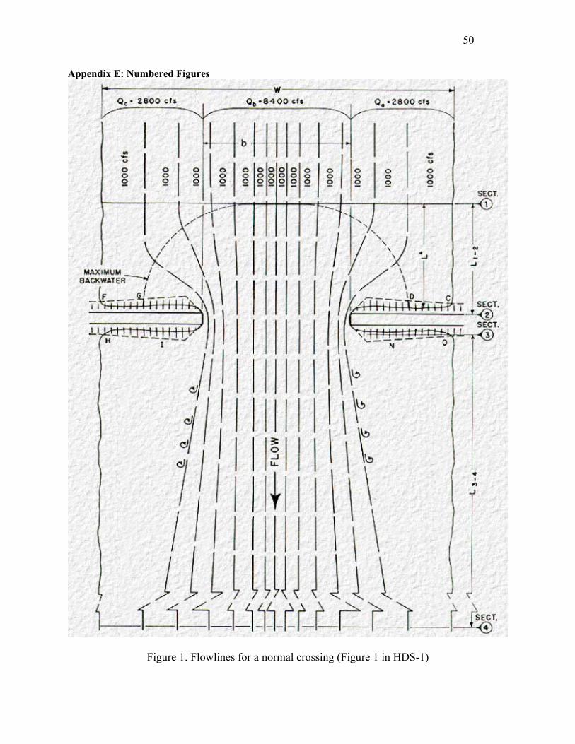
50

Appendix E: Numbered Figures

Figure 1. Flowlines for a normal crossing (Figure 1 in HDS-1)

51

Figure 2. Normal crossings: Spillthrough abutments (Figure 3 in HDS-1)

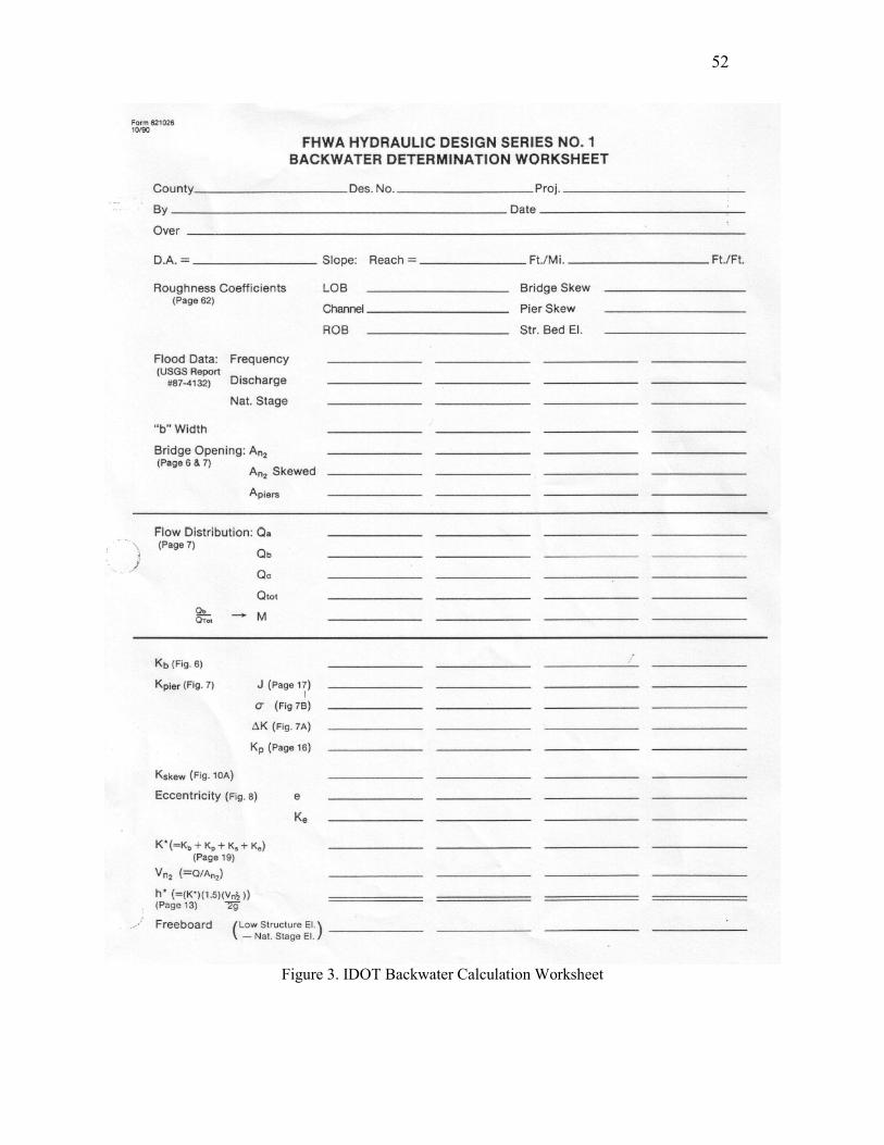
52

Figure 3. IDOT Backwater Calculation Worksheet

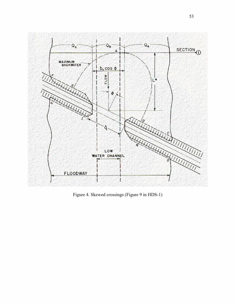
53

Figure 4. Skewed crossings (Figure 9 in HDS-1)

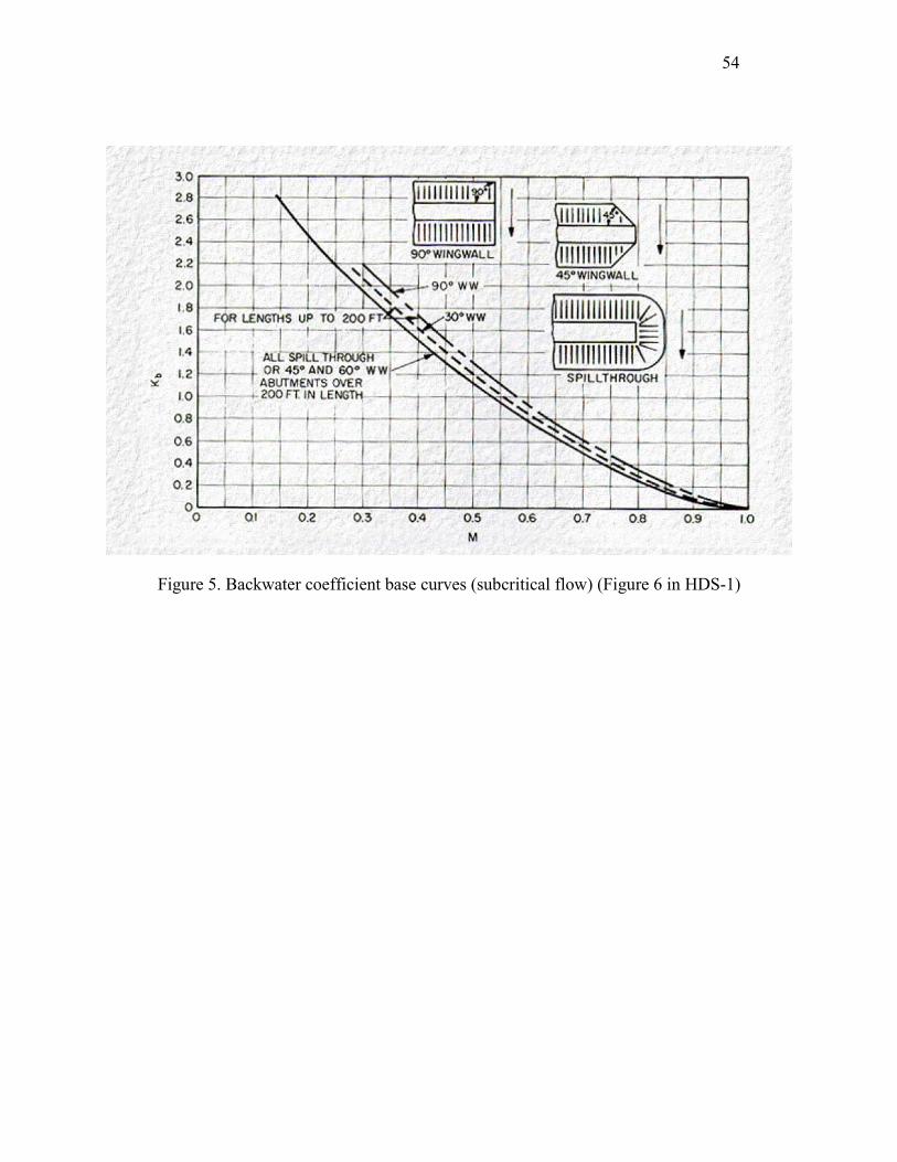
54

Figure 5. Backwater coefficient base curves (subcritical flow) (Figure 6 in HDS-1)

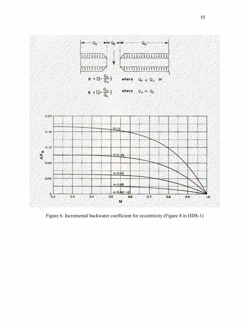
55

Figure 6. Incremental backwater coefficient for eccentricity (Figure 8 in HDS-1)

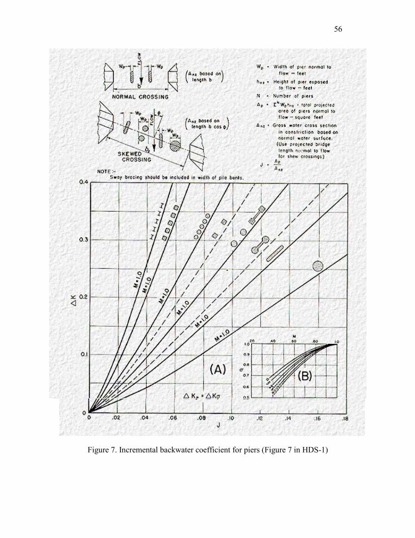
56

Figure 7. Incremental backwater coefficient for piers (Figure 7 in HDS-1)

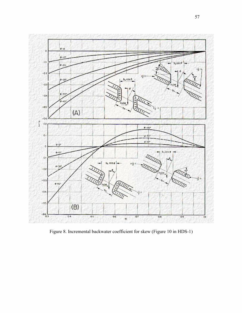
57

Figure 8. Incremental backwater coefficient for skew (Figure 10 in HDS-1)

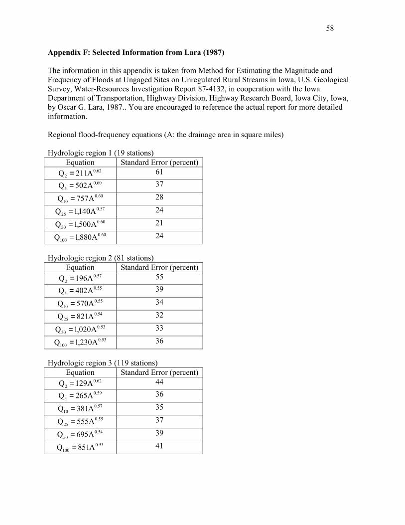
58

Appendix F: Selected Information from Lara (1987) The information in this appendix is taken from Method for Estimating the Magnitude and Frequency of Floods at Ungaged Sites on Unregulated Rural Streams in Iowa, U.S. Geological Survey, Water-Resources Investigation Report 87-4132, in cooperation with the Iowa Department of Transportation, Highway Division, Highway Research Board, Iowa City, Iowa, by Oscar G. Lara, 1987.. You are encouraged to reference the actual report for more detailed information. Regional flood-frequency equations (A: the drainage area in square miles) Hydrologic region 1 (19 stations)

Equation Standard Error (percent) 62.0

2 A211Q = 61 60.0

5 A502Q = 37 60.0

10 A757Q = 28 57.0

25 A140,1Q = 24 60.0

50 A500,1Q = 21 60.0

100 A880,1Q = 24 Hydrologic region 2 (81 stations)

Equation Standard Error (percent) 57.0

2 A196Q = 55 55.0

5 A402Q = 39 55.0

10 A570Q = 34 54.0

25 A821Q = 32 53.0

50 A020,1Q = 33 53.0

100 A230,1Q = 36

Hydrologic region 3 (119 stations) Equation Standard Error (percent)

62.02 A129Q = 44

59.05 A265Q = 36

57.010 A381Q = 35

55.025 A555Q = 37

54.050 A695Q = 39

53.0100 A851Q = 41

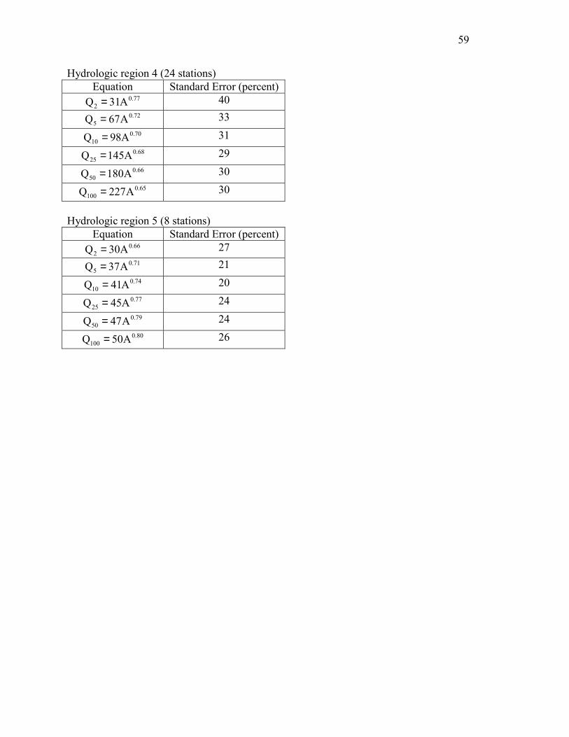
59

Hydrologic region 4 (24 stations) Equation Standard Error (percent)

77.02 A31Q = 40

72.05 A67Q = 33

70.010 A98Q = 31

68.025 A145Q = 29

66.050 A180Q = 30

65.0100 A227Q = 30

Hydrologic region 5 (8 stations)

Equation Standard Error (percent) 66.0

2 A30Q = 27 71.0

5 A37Q = 21 74.0

10 A41Q = 20 77.0

25 A45Q = 24 79.0

50 A47Q = 24 80.0

100 A50Q = 26

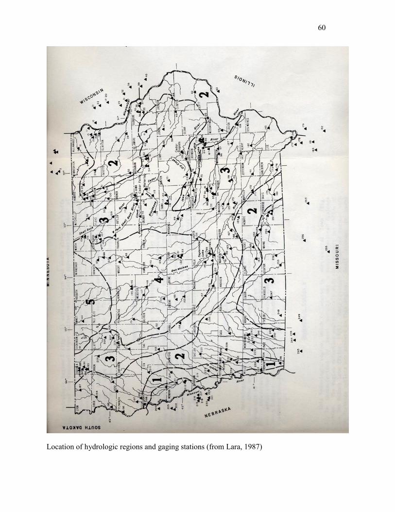
60

Location of hydrologic regions and gaging stations (from Lara, 1987)

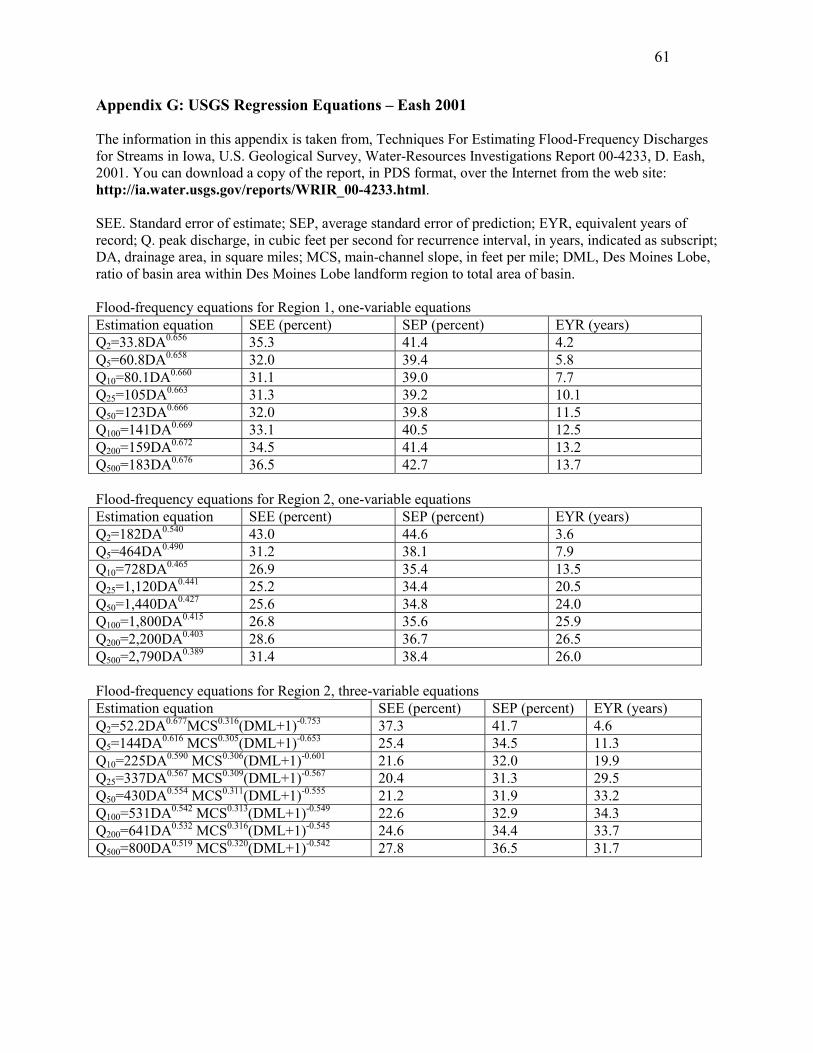
61

Appendix G: USGS Regression Equations – Eash 2001 The information in this appendix is taken from, Techniques For Estimating Flood-Frequency Discharges for Streams in Iowa, U.S. Geological Survey, Water-Resources Investigations Report 00-4233, D. Eash, 2001. You can download a copy of the report, in PDS format, over the Internet from the web site: http://ia.water.usgs.gov/reports/WRIR_00-4233.html. SEE. Standard error of estimate; SEP, average standard error of prediction; EYR, equivalent years of record; Q. peak discharge, in cubic feet per second for recurrence interval, in years, indicated as subscript; DA, drainage area, in square miles; MCS, main-channel slope, in feet per mile; DML, Des Moines Lobe, ratio of basin area within Des Moines Lobe landform region to total area of basin. Flood-frequency equations for Region 1, one-variable equations Estimation equation SEE (percent) SEP (percent) EYR (years) Q2=33.8DA0.656 35.3 41.4 4.2 Q5=60.8DA0.658 32.0 39.4 5.8 Q10=80.1DA0.660 31.1 39.0 7.7 Q25=105DA0.663 31.3 39.2 10.1 Q50=123DA0.666 32.0 39.8 11.5 Q100=141DA0.669 33.1 40.5 12.5 Q200=159DA0.672 34.5 41.4 13.2 Q500=183DA0.676 36.5 42.7 13.7 Flood-frequency equations for Region 2, one-variable equations Estimation equation SEE (percent) SEP (percent) EYR (years) Q2=182DA0.540 43.0 44.6 3.6 Q5=464DA0.490 31.2 38.1 7.9 Q10=728DA0.465 26.9 35.4 13.5 Q25=1,120DA0.441 25.2 34.4 20.5 Q50=1,440DA0.427 25.6 34.8 24.0 Q100=1,800DA0.415 26.8 35.6 25.9 Q200=2,200DA0.403 28.6 36.7 26.5 Q500=2,790DA0.389 31.4 38.4 26.0 Flood-frequency equations for Region 2, three-variable equations Estimation equation SEE (percent) SEP (percent) EYR (years) Q2=52.2DA0.677MCS0.316(DML+1)-0.753 37.3 41.7 4.6 Q5=144DA0.616 MCS0.305(DML+1)-0.653 25.4 34.5 11.3 Q10=225DA0.590 MCS0.306(DML+1)-0.601 21.6 32.0 19.9 Q25=337DA0.567 MCS0.309(DML+1)-0.567 20.4 31.3 29.5 Q50=430DA0.554 MCS0.311(DML+1)-0.555 21.2 31.9 33.2 Q100=531DA0.542 MCS0.313(DML+1)-0.549 22.6 32.9 34.3 Q200=641DA0.532 MCS0.316(DML+1)-0.545 24.6 34.4 33.7 Q500=800DA0.519 MCS0.320(DML+1)-0.542 27.8 36.5 31.7

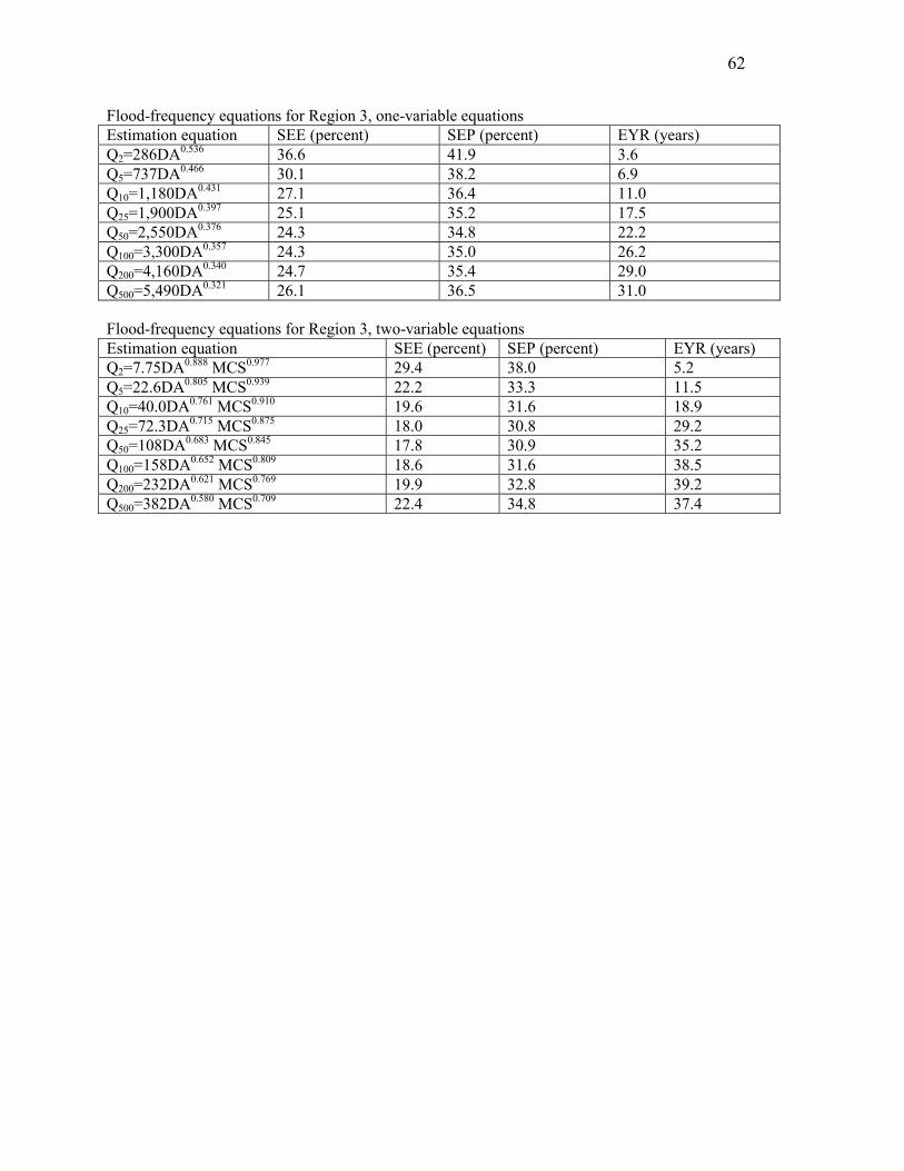
62

Flood-frequency equations for Region 3, one-variable equations Estimation equation SEE (percent) SEP (percent) EYR (years) Q2=286DA0.536 36.6 41.9 3.6 Q5=737DA0.466 30.1 38.2 6.9 Q10=1,180DA0.431 27.1 36.4 11.0 Q25=1,900DA0.397 25.1 35.2 17.5 Q50=2,550DA0.376 24.3 34.8 22.2 Q100=3,300DA0.357 24.3 35.0 26.2 Q200=4,160DA0.340 24.7 35.4 29.0 Q500=5,490DA0.321 26.1 36.5 31.0 Flood-frequency equations for Region 3, two-variable equations Estimation equation SEE (percent) SEP (percent) EYR (years) Q2=7.75DA0.888 MCS0.977 29.4 38.0 5.2 Q5=22.6DA0.805 MCS0.939 22.2 33.3 11.5 Q10=40.0DA0.761 MCS0.910 19.6 31.6 18.9 Q25=72.3DA0.715 MCS0.875 18.0 30.8 29.2 Q50=108DA0.683 MCS0.845 17.8 30.9 35.2 Q100=158DA0.652 MCS0.809 18.6 31.6 38.5 Q200=232DA0.621 MCS0.769 19.9 32.8 39.2 Q500=382DA0.580 MCS0.709 22.4 34.8 37.4

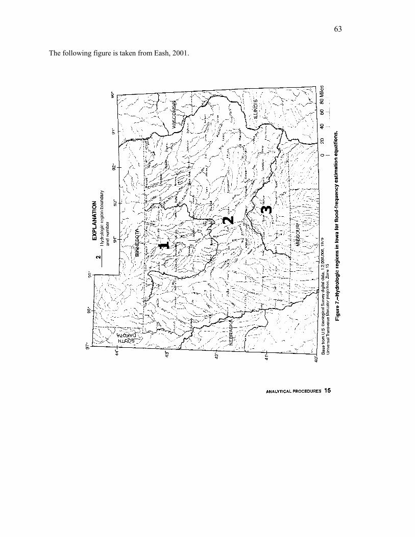
63

The following figure is taken from Eash, 2001.

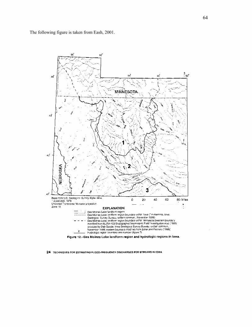
64

The following figure is taken from Eash, 2001.