is it worth it? quantifying the value of risk-managed · pdf fileis it worth it? quantifying...

Is It Worth It?

Quantifying the Value of Risk-Managed Investing

By Jerry Miccolis, CFA®, CFP®, FCAS, MAAA, CERA; Marina Goodman, CFA®, CFP®; Rohith Eggidi

Executive Summary

To meet their long-range financial goals, most investors need a sizeable allocation to

“risk assets” such as equities in their portfolio, but large drawdowns in these assets are

quite frequent. The S&P 500 Total Return Index, for example, has suffered drawdowns

of -10% or worse 29 times since 1935, a frequency of once every 2.7 years on average.

Risk-managed investing (RMI) attempts to take traditional portfolio management —

typified by diversification, asset allocation, and rebalancing — to the next level by

explicitly dampening portfolio volatility and/or limiting downside potential.

This paper addresses fundamental questions about RMI, including why it should be

considered, and how low its cost needs to be to add long-term value.

Qualitative considerations and an array of quantitative demonstrations document the

potential economic value of RMI.

Volatility-dampening is shown to add value by reducing risk drag, mitigating sequence

risk, exploiting tax effects, and capturing the economic benefit long recognized by

institutional investors.

Downside protection is shown to add value by taking advantage of return asymmetry;

even a modestly effective RMI strategy can support a cost — in terms of performance

drag in rising markets — of several hundred basis points of return per year.

The quantitative techniques in the paper can be used by investment professionals to

objectively test the efficacy of proposed RMI solutions in the marketplace.

Is It Worth It?


Introduction

There is considerable interest throughout the investment community in the subject of portfolio

risk management. And much debate.

Some believe that going beyond traditional approaches — primarily, strategic asset allocation

and rebalancing — to more explicitly manage portfolio risk may be the next great conceptual

breakthrough in the science and practice of investment management. Others maintain that this

attempt — whether through tactical portfolio adjustments, quantitative strategies, or

sophisticated hedging techniques — is a waste of time and effort, and may mislead a

susceptible public. The risk management advocates typically base their belief on the premise

that improving the risk/return profile of a portfolio is always in the long-term best interests of

the investor. The skeptics argue that the costs of risk management — both direct costs and the

apparent need to sacrifice some upside potential — are doomed to make the whole enterprise

a breakeven proposition, or worse.

In recent years, there has been a proliferation of products and solutions that have made

attempts at explicit investment risk management, and depending upon which of those you

examine, either side of the debate can be right. This paper will not address any particular

product or solution. Instead, it will address the question more broadly and conceptually, but

also with quantitative rigor, so that the efficacy of any proposed solution might be assessed in

an informed, objective way.

Specifically, in this paper we will critically evaluate the rationale for considering risk-managed

investing (RMI). In the process, we will attempt to quantify the economic value, if any, of

improving the return stream of an investment or portfolio by:

Dampening its volatility; and/or

Limiting its downside potential.

Through this quantification, we will estimate an upper bound on the acceptable cost of RMI

devices aimed at delivering these improvements.

Is It Worth It?


We hope that this paper helps establish a sound scientific foundation for investment

professionals to fairly evaluate developments in this critical area.

Fundamental Questions

Much of the dialogue on risk-managed investing (RMI) can be captured in three key questions:

Why should I consider it?

How much should I be willing to pay for it?

If I have a long-term investment horizon and little concern for short-term volatility, is it

even relevant to me?

So, let’s address them directly.

Reasons One Might Consider Risk-Managed Investing

As it turns out, there are a number of compelling reasons, both qualitative and quantitative,

that a prudent investor might wish to explore RMI.

On the qualitative side, many investors place high emotional value on predictability and peace

of mind, often above most other considerations. This, by itself, may be sufficient cause for

some people to embrace RMI. But there is also a much broader group of people for whom a

similar sentiment more subtly holds sway.

Virtually all investors, however conservative or aggressive, need a healthy dose of “risk assets”

(see note1) in their portfolio. Why? Because higher-risk investments tend to carry higher-

return expectations. And without them, the low-risk/low-return investments that are left are

simply not, in general, sufficient to preserve the purchasing power of the portfolio. In other

words, the actual economic value of the portfolio, even if its nominal value stays stable or

slightly increases, will tend to decline over time as inflation eats away at it. Inflation may not

1 We will use “risk assets” to denote any asset that exhibits volatility higher than that of cash and investment grade

bonds. Risk assets typically include equities, real estate, commodities, and other alternative investments.

Is It Worth It?


seem like much at any given moment, but over the time horizon of most investors — which is

measured in decades — inflation is the single biggest financial threat they face.

The best defense (and offense) against inflation? Risk assets. A well-diversified portfolio held

over a long period can help investors capture the high returns associated with risk assets while

mitigating their risks at the portfolio level. Indeed, that is the whole point behind asset

allocation. But, many investors simply cannot tolerate the volatility in those risk assets long

enough for the benefits to play out. Their fear of uncertainty denies them access to one of the

most potent tools they have to best secure their financial future.

RMI can be a way for these investors to become comfortable enough with risk assets that they

will stick with them when they should. It can help these individuals control their fear, and let

asset allocation work for them. The value of that result, while qualitative, can be immense.

That last statement cannot be overemphasized. Consider, for example, that some investors

were so traumatized by the market collapse of late 2008/early 2009 that they exited the

markets altogether in 2009. By the time they returned, long into the inevitable rebound, they

had forfeited forever the “wealth re-creation” that the markets delivered to those who stayed

the course. If RMI had helped keep those investors from making ill-informed, fear-driven

decisions, the positive difference in their long-term financial future would have been enormous

— of a magnitude that might easily outstrip any other impact we discuss in this paper.

There is another consideration in the qualitative realm, though this is more of a stretch. To the

extent that someone is comfortable that the risk to his/her nest egg is well managed, to the

point of supreme sleep-at-night serenity, then that person may be more willing to explore and

undertake unrelated prudently-risky endeavors that may have high-reward potential in his/her

life or career. Fear can be limiting; lack of fear can be liberating, and foster higher quality of

life.

Is It Worth It?


Quantitative Considerations — Volatility-Dampening

Let’s tackle the quantitative side of the discussion in two parts. We’ll first assess the economic

value of volatility-dampening. We’ll then do the same for downside protection.

A Very Simple Example

What’s better, a stable 8% return or a volatile 9%? The answer, as you might imagine, depends

on how volatile the 9% is. In the simple example below (Exhibit 1), we compare a rock-steady

8% annual return with a fairly erratic return stream that happens to average 9%.

Exhibit 1

The 9%-return portfolio results in lower ending wealth than the 8%-return portfolio. It seems

clear from this that there is demonstrable economic value in stability of returns. This can be

quantified more generally.

The mathematically astute reader may recognize the difference between the 9.0% average

return and the 7.6% compound annual return in Portfolio B of the above example as the

difference between the arithmetic mean return (AMR) and the geometric mean return (GMR),

Portfolio A Portfolio B

Annual Account Annual Account

Return Balance Return Balance

Beginning Balance $100 $100

Year 1 8% $108 23% $123

Year 2 8% $117 -14% $106

Year 3 8% $126 -7% $98

Year 4 8% $136 20% $118

Year 5 8% $147 16% $137

Year 6 8% $159 14% $156

Year 7 8% $171 -18% $127

Year 8 8% $185 27% $162

Year 9 8% $200 -2% $158

Year 10 8% $216 32% $208

Ending Balance $216 $208

Average Return 8.0% 9.0%

Compound Annual Return 8.0% 7.6%

Standard Deviation 0.0% 18.0%

Is It Worth It?


respectively. GMR is the measure that corresponds to ending wealth, and so should be the

measure most relevant to investors. It is a mathematical fact that, for a given return stream,

GMR is always less than or equal to AMR. The difference between the two grows with volatility

(a phenomenon some call “risk drag”), and a crude approximation formula is GMR ≈ AMR – V/2,

where V is the variance (standard deviation squared) of the return stream (see note2).

Thus, if volatility can be dampened (i.e., if the V in the approximation formulas can be reduced),

we can calculate the value added very directly, in terms of increased compound return (GMR)

and, therefore, ending wealth.

Sequence Risk

Return stability has additional economic benefits. One relates to a phenomenon called

“sequence risk.” Sequence risk occurs when the specific sequence of periodic returns is such

that it impairs the financial condition of the investor, relative to a more favorable sequence of

the same periodic returns.

Suppose, for example, that a severe market downturn occurs immediately before the investor

needs to make a significant portfolio withdrawal to cover a major living expense, such as a

house purchase. This has worse long-term consequences than if the downturn occurred after

the withdrawal. In the first case, the investor had to withdraw a larger percentage of the now-

diminished portfolio than he/she would otherwise have needed to, leaving relatively fewer

assets in the portfolio to enjoy any subsequent market recovery. In the second case, the

withdrawal actually protected a meaningful part of the portfolio from harm, and the house was

purchased with “pre-depreciated” assets.

2

See, for example, Diversification, Rebalancing, and the Geometric Mean Frontier, William J. Bernstein and David Wilkinson (1997) and On the Relationship between Arithmetic and Geometric Returns, Dimitry Mindlin (2011), which also offer the following approximations (using Excel notation):

GMR ≈ AMR – V / (2*(1 + AMR)), and

GMR ≈ (1 + AMR)*(1 + V*(1 + AMR)^(-2))^(-0.5) - 1 Another is: GMR ≈ (1 + AMR)*(1 + V/(1 + AMR)^2)^((1-N)/(2*N)) - 1, where N is the number of compounding periods.

Is It Worth It?


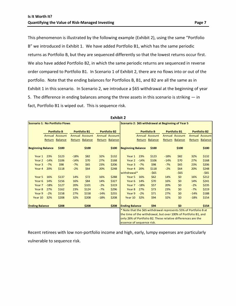
This phenomenon is illustrated by the following example (Exhibit 2), using the same “Portfolio

B” we introduced in Exhibit 1. We have added Portfolio B1, which has the same periodic

returns as Portfolio B, but they are sequenced differently so that the lowest returns occur first.

We also have added Portfolio B2, in which the same periodic returns are sequenced in reverse

order compared to Portfolio B1. In Scenario 1 of Exhibit 2, there are no flows into or out of the

portfolio. Note that the ending balances for Portfolios B, B1, and B2 are all the same as in

Exhibit 1 in this scenario. In Scenario 2, we introduce a $65 withdrawal at the beginning of year

5. The difference in ending balances among the three assets in this scenario is striking — in

fact, Portfolio B1 is wiped out. This is sequence risk.

Exhibit 2

Recent retirees with low non-portfolio income and high, early, lumpy expenses are particularly

vulnerable to sequence risk.

Scenario 1: No Portfolio Flows Scenario 2: $65 withdrawal at Beginning of Year 5

Portfolio B Portfolio B1 Portfolio B2 Portfolio B Portfolio B1 Portfolio B2

Annual Account Annual Account Annual Account Annual Account Annual Account Annual Account

Return Balance Return Balance Return Balance Return Balance Return Balance Return Balance

Beginning Balance $100 $100 $100 Beginning Balance $100 $100 $100

Year 1 23% $123 -18% $82 32% $132 Year 1 23% $123 -18% $82 32% $132

Year 2 -14% $106 -14% $70 27% $168 Year 2 -14% $106 -14% $70 27% $168

Year 3 -7% $98 -7% $65 23% $206 Year 3 -7% $98 -7% $65 23% $206

Year 4 20% $118 -2% $64 20% $248 Year 4 20% $118 -2% $64 20% $248

withdrawal* -$65 -$65 -$65

Year 5 16% $137 14% $72 16% $288 Year 5 16% $62 14% $0 16% $212

Year 6 14% $156 16% $84 14% $327 Year 6 14% $70 16% $0 14% $241

Year 7 -18% $127 20% $101 -2% $319 Year 7 -18% $57 20% $0 -2% $235

Year 8 27% $162 23% $124 -7% $296 Year 8 27% $73 23% $0 -7% $219

Year 9 -2% $158 27% $158 -14% $255 Year 9 -2% $71 27% $0 -14% $188

Year 10 32% $208 32% $208 -18% $208 Year 10 32% $94 32% $0 -18% $154

Ending Balance $208 $208 $208 Ending Balance $94 $0 $154

* Note that the $65 withdrawal represents 55% of Portfolio B at

the time of the withdrawal, but over 100% of Portfolio B1, and

only 26% of Portfolio B2. These relative differences are the

essence of sequence risk.

Is It Worth It?


There are a few ways to mitigate sequence risk. One is to have no flows — deposits or

withdrawals — into or out of the portfolio (see note3). But this is patently unrealistic for most

investors. Another way is to successfully avoid making withdrawals for a time after a significant

decline in the portfolio’s value. This might be accomplished by keeping a sizeable cash reserve

outside the portfolio to cover this contingency. However, the size of the reserve necessary to

achieve meaningful immunization against contingencies of unknown frequency and severity is

large that the long-term “cash drag” on performance tends to outweigh the benefits, as a

number of studies in the financial literature have demonstrated (see note4).

The most productive way to control sequence risk is to not have an erratic series of returns —

the more stable the return stream, the less the sequence risk. A perfectly smooth return

stream, such as that of Portfolio A in Exhibit 1, has precisely zero sequence risk. (This is a given,

since all sequencings of identical periodic returns are indistinguishable from each other.) It

does not matter when deposits or withdrawals occur in such a portfolio. While no practical RMI

technique can totally eliminate return volatility, every step in that direction adds value from a

sequence risk perspective.

To recap, the value of stability to mitigate sequence risk is very clear, and can be quantified

using the approach in Exhibit 2.

Tax Effects

If the investments in question are in a taxable account, and the investor is subject (as in the

U.S.) to a progressive tax rate structure, then there may be additional quantitative value in

stability. Without getting into the vagaries of the tax code (and the treatment of different

categories of gains and income, let alone deductions, loss carry-forwards, etc., etc.), this value

3 By the way, we have found that this is not well understood, even by professional investors. If there are no flows

into or out of the portfolio, the sequence of returns does not matter — there is no effect on ending wealth. This should be clear from Scenario 1 of Exhibit 2. In fact, you can rearrange the sequence of returns in any way you like, and you will get the identical end result. 4 See, for example, "Sustainable Withdrawal Rates: The Historical Evidence on Buffer Zone Strategies" by Walter

Woerheide and David Nanigan, Journal of Financial Planning, May 2012; and “Research Reveals Cash Reserve Strategies Don't Work... Unless You're A Good Market Timer” by Michael Kitces, Retirement Planning, June 2012.

http://www.fpanet.org/journal/Home/SustainableWithdrawalRates/

http://www.kitces.com/blog/archives/341-Research-Reveals-Cash-Reserve-Strategies-Dont-Work...-Unless-Youre-A-Good-Market-Timer.html

http://www.kitces.com/blog/archives/341-Research-Reveals-Cash-Reserve-Strategies-Dont-Work...-Unless-Youre-A-Good-Market-Timer.html

Is It Worth It?


is readily appreciated by considering that downward deviations in investment returns save less

in avoided tax liabilities than upward deviations generate in additional tax liabilities. The

example below (Exhibit 3) illustrates this effect, using two three-year return streams that each

total the same pre-tax amount — one stable, and one volatile. The stable return stream

generates a higher after-tax result.

Exhibit 3

Since tax effects are very specific to each individual, generic quantification cannot be done. All

that can be said in a tax context is that the economic benefit provided by stability is non-

negative, and can be considered “icing on the cake.”

Institutional Investor Perspectives

There are a number of quantitative studies of institutional investor behavior that support the

premise that return stability adds economic value.

The Casualty Actuarial Society (see note5) has attempted to quantify the value of risk

management in a number of ways. We will not recite the various methodologies here, but

suffice it to say that the notion of risk management providing economic value is rigorously

established.

5 See, for example, Assessing the Value of Risk Reduction, Gary Venter and Alice Underwood, Casualty Actuarial

Society (2014).

Stable Return Stream Volatile Return Stream

Investment Income Net Investment Income Net

Gain Tax Result Gain Tax Result

Year 1 $100 $15 $85 $100 $15 $85

Year 2 $100 $15 $85 $50 $5 $45

Year 3 $100 $15 $85 $150 $30 $120

3-Year Total $300 $45 $255 $300 $50 $250

hypothetical tax rate table:

10% of first $50

20% of next $50

30% of excess

Is It Worth It?


In studies conducted by the international consulting firm Towers Perrin (see note6), it was

documented that publicly traded companies that exhibited stable earnings enjoyed higher

relative market valuations than companies that did not, even after normalizing for other

valuation drivers such as return on capital and earnings growth. This, despite the conventional

notion that such stability is not assigned positive value by the market under the premise that

single-company volatility can be diversified away.

These studies, and others like them, repeatedly demonstrate that knowledgeable investors

indeed place measurable value on volatility dampening.

Quantitative Considerations — Downside Protection

If more stable returns — which enjoy both upside and downside volatility dampening — add

demonstrable value, then it stands to reason that a return stream with strictly downside

dampening should add even more value, as upside variations remain unimpeded. This

proposition is dealt with in the balance of this paper.

Return Asymmetry

Let’s start very simply. It is a well-known but underappreciated fact that positive and negative

returns are asymmetric — that is, every -1% decline requires greater than a +1% recovery to get

the investor back to break-even. On an initial investment of $100, for example, a -10% loss (to

$90) requires a subsequent +11% gain ($100/$90 – 1) to get back to $100. The larger the

percentage, the more pronounced the asymmetry. This is generalized in the following table

(Exhibit 4).

6 See, for example RiskValueInsights: Creating Value Through Enterprise Risk Management, a Tillinghast—Towers

Perrin monograph (2002).

Is It Worth It?


Exhibit 4

The immediate takeaway from this observation is that it is more valuable to avoid a decline

than it is to capture a gain of the same magnitude. This has major ramifications, which we

explore below.

A Look at Equity Market History

The capital markets are characterized by recurring periods of decline and recovery. Taking the

U.S. equity market, as represented by the S&P 500 Total Return Stock Index, as our example in

this section, the long-term average annual return is approximately +10.5%. This overall upward

tendency has been interrupted fairly often by periods of substantial decline.

As the Appendix and Exhibit 5 below show, over the 78-year period from the beginning of 1936

through the end of 2013, there have been 29 separate, non-overlapping episodes of market

declines that were each worse than -10%. Note that this equates to a frequency of once every

2.7 years, on average.

negative necessary offsetting

return positive return

-10% +11%

-20% +25%

-30% +43%

-40% +67%

-50% +100%

Is It Worth It?


Exhibit 5

The average decline during those peak-to-trough periods (the red regions of Exhibit 5) has been

approximately -21%, and the average episode has persisted for about eight months.

Representatively, the subsequent trough-to-peak upswing (the combined light- and dark-green

regions of the exhibit) has been roughly +65% cumulatively, and has lasted around 24 months

(i.e., before the next -10%-or-worse downswing began) (see note7). Assuming a $100.00 initial

investment in this market at the beginning of a representative downdraft, it would decline to

$79.00 over the first eight months, and then rebound to $130.35 over the next 24 months.

Note, as a consistency check, that these figures are consistent with a long-term annual average

return of approximately +10.5%, as cited above (see note8).

Quantifying the Impact of RMI Strategies

Now let’s consider a downside RMI strategy that succeeds in modestly reducing the decline on

the initial $100.00 investment, from -21% to -15.5% (i.e., by half the excess decline beyond -

10%), net of the cost of the strategy. In that case, if the subsequent +65% upturn is unimpeded, 7 Does the average 32-month term of the full cycle sound short? It initially did to us. But if it were any longer,

there could not have been 29 of them in the last 78 years. 8 Using Excel notation: ((1 - 0.21)*(1 + 0.65))^(12/(8+24)) - 1 ≈ 0.105.

Alternatively, ($130.35/$100.00) ^(12/(8+24)) - 1 ≈ 0.105

1

10

100

1000

10000

100000

-60%

-50%

-40%

-30%

-20%

-10%

0%

S&P

50

0 T

/R In

dex

-Lo

g S

cale

Dra

wd

ow

n

Peak to Trough Trough to Recovery Recovery to Next Peak Drawdown (left scale)

Is It Worth It?


the result after the full 32-month cycle would be $139.43, a much better result than $130.35,

and one that would imply a long-term average annual return of +13.3% instead of +10.5%.

Here is the interesting, and most practical, part. It is unrealistic to assume that an RMI strategy

could successfully reduce the downside, however modestly, and not have some cost, in terms

of a performance drag on the upside. The simple 32-month model above gives us an excellent

way to estimate how large that upside performance drag could be without negating the benefit

of the downside protection. Specifically, if the 8-month decline on the $100.00 investment is -

15.5% (net of the cost of the strategy) instead of -21%, then the subsequent 24-month bull

market run need only be +54.3% cumulatively instead of +65% to achieve the breakeven value

of $130.35.

What does the above result mean in terms of the annual tolerable cost? Well, the annualized

version of the +65% 24-month return is +28.5%, while the annualized version of the +54.3%

return is +24.2%. The difference is 425 basis points. So, finally, here is the result we’ve been

seeking: an RMI strategy that reduces only large declines in the equity markets (i.e., those

worse than -10%), and reduces them only modestly (i.e., by half their excess beyond -10%),

adds measurable value as long as its cost (i.e., its performance drag during bull markets) does

not exceed 425 basis points per annum. This kind of RMI strategy is not a stretch by any

means — it is quite realistically achievable. RMI strategies such as this seem well worth

pursuing.

To give some additional texture to this result, consider an RMI strategy that reduces the impact

of portfolio downturns by 50% of the excess downturn beyond -10% (as in the example above)

whose cost amounts to an annual performance drag of 325 basis points — that is, 100 basis

points better than the 425 basis point breakeven level derived above. And consider its impact

over the investment horizon of a newly-married couple just leaving college. The probability of

at least one spouse living into his/her late nineties is sizeable enough that prudent financial

planning should consider a horizon of 75 to 80 years. If these years are anything like the last 78

Is It Worth It?


years, every dollar invested by the newlyweds in the RMI portfolio will have grown to roughly

twice as much as it would have in a non-RMI portfolio over that horizon.

Generalizing the Results

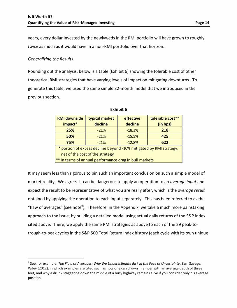
Rounding out the analysis, below is a table (Exhibit 6) showing the tolerable cost of other

theoretical RMI strategies that have varying levels of impact on mitigating downturns. To

generate this table, we used the same simple 32-month model that we introduced in the

previous section.

Exhibit 6

It may seem less than rigorous to pin such an important conclusion on such a simple model of

market reality. We agree. It can be dangerous to apply an operation to an average input and

expect the result to be representative of what you are really after, which is the average result

obtained by applying the operation to each input separately. This has been referred to as the

“flaw of averages” (see note9). Therefore, in the Appendix, we take a much more painstaking

approach to the issue, by building a detailed model using actual daily returns of the S&P index

cited above. There, we apply the same RMI strategies as above to each of the 29 peak-to-

trough-to-peak cycles in the S&P 500 Total Return Index history (each cycle with its own unique

9 See, for example, The Flaw of Averages: Why We Underestimate Risk in the Face of Uncertainty, Sam Savage,

Wiley (2012), in which examples are cited such as how one can drown in a river with an average depth of three feet, and why a drunk staggering down the middle of a busy highway remains alive if you consider only his average position.

RMI downside

impact*

typical market

decline

effective

decline

tolerable cost**

(in bps)

25% -21% -18.3% 218

50% -21% -15.5% 425

75% -21% -12.8% 622

* portion of excess decline beyond -10% mitigated by RMI strategy,

net of the cost of the strategy

** in terms of annual performance drag in bull markets

Is It Worth It?


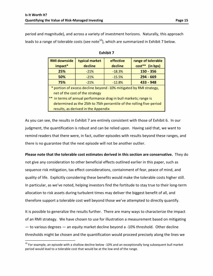
period and magnitude), and across a variety of investment horizons. Naturally, this approach

leads to a range of tolerable costs (see note10), which are summarized in Exhibit 7 below.

Exhibit 7

As you can see, the results in Exhibit 7 are entirely consistent with those of Exhibit 6. In our

judgment, the quantification is robust and can be relied upon. Having said that, we want to

remind readers that there were, in fact, outlier episodes with results beyond these ranges, and

there is no guarantee that the next episode will not be another outlier.

Please note that the tolerable cost estimates derived in this section are conservative. They do

not give any consideration to other beneficial effects outlined earlier in this paper, such as

sequence risk mitigation, tax effect considerations, containment of fear, peace of mind, and

quality of life. Explicitly considering these benefits would make the tolerable costs higher still.

In particular, as we’ve noted, helping investors find the fortitude to stay true to their long-term

allocation to risk assets during turbulent times may deliver the biggest benefit of all, and

therefore support a tolerable cost well beyond those we’ve attempted to directly quantify.

It is possible to generalize the results further. There are many ways to characterize the impact

of an RMI strategy. We have chosen to use for illustration a measurement based on mitigating

— to various degrees — an equity market decline beyond a -10% threshold. Other decline

thresholds might be chosen and the quantification would proceed precisely along the lines we

10

For example, an episode with a shallow decline below -10% and an exceptionally long subsequent bull market period would lead to a tolerable cost that would be at the low end of the range.

RMI downside

impact*

typical market

decline

effective

decline

range of tolerable

cost** (in bps)

25% -21% -18.3% 150 - 356

50% -21% -15.5% 294 - 669

75% -21% -12.8% 433 - 948

* portion of excess decline beyond -10% mitigated by RMI strategy,

net of the cost of the strategy

** in terms of annual performance drag in bull markets; range is

determined as the 25th to 75th percentile of the rolling five-period

results, as derived in the Appendix

Is It Worth It?


have outlined above (see note11). Some RMI techniques, however, may not lend themselves to

measurement along those lines. For example, some may follow the same general risk

management approach (i.e., protection beyond a threshold), but their impact may be less

precise or certain than implied above. Those situations can easily be modeled following our

example — that is, by applying the strategy directly to the relevant historical episodes and

deriving the tolerable performance drag during the succeeding or preceding bull market period.

Whichever way a particular RMI strategy may deliver its mitigating effect, we hope our

quantification approach provides a rough roadmap to measuring the economic value of that

effect.

Summary and Conclusions

Let’s return to our fundamental questions, and recap our answers to them.

Why should I consider RMI? We uncovered a number of qualitative reasons to strongly

consider RMI. Whether the RMI strategies under review have impact on dampening portfolio

volatility, limiting downside potential, or both, these reasons include predictability, peace of

mind, fortitude to fight inflation with higher-risk assets, freedom to take other prudent chances

in life and career, success in mitigating sequence risk, and opportunity to minimize tax effects.

Sophisticated institutional investors concur that RMI has material value. We also documented

an array of quantitative analyses to demonstrate the value of RMI.

How much should I be willing to pay for RMI? The detailed quantitative modeling we have done

indicates that a cost of several hundred basis points per year, in terms of performance drag

during bull markets, is justified by RMI. The tolerable cost can be calibrated specifically,

depending on the mitigating impact a particular RMI strategy may have on downside market

moves. The non-quantified, but very real, qualitative benefits outlined above render this

calibration conservative.

11

Directionally, at least, those results can be predicted. At the risk of stating the obvious, a threshold of -5% instead of -10%, for example, would lead to higher tolerable cost levels, while a threshold of -15% would result in lower levels.

Is It Worth It?


If I have a long-term investment horizon and little concern for short-term volatility, is RMI even

relevant to me? In a word, yes. Even the most aggressive investor, who does not customarily

view investments through a risk-management lens, should be interested in an approach that

increases long-term returns, as RMI can. Moreover, since the value of RMI is realized most fully

over several bull-and-bear market cycles, the longer an investor’s investment horizon, the more

value is potentially added by RMI.

We hope that, with this paper, we have helped establish a solid foundation for the fair

evaluation of products and solutions that have been, and will be, brought to market in this

important area.

Based on our work to date, it is our firm conclusion that RMI should be utilized as a potent

weapon in the arsenal of every serious investment professional.

Is It Worth It?


APPENDIX — Historical Model

To provide the raw data to support the quantitative analyses of downside protection, we

compiled the history of one of the longest-recorded and most-closely-followed risk assets, U.S.

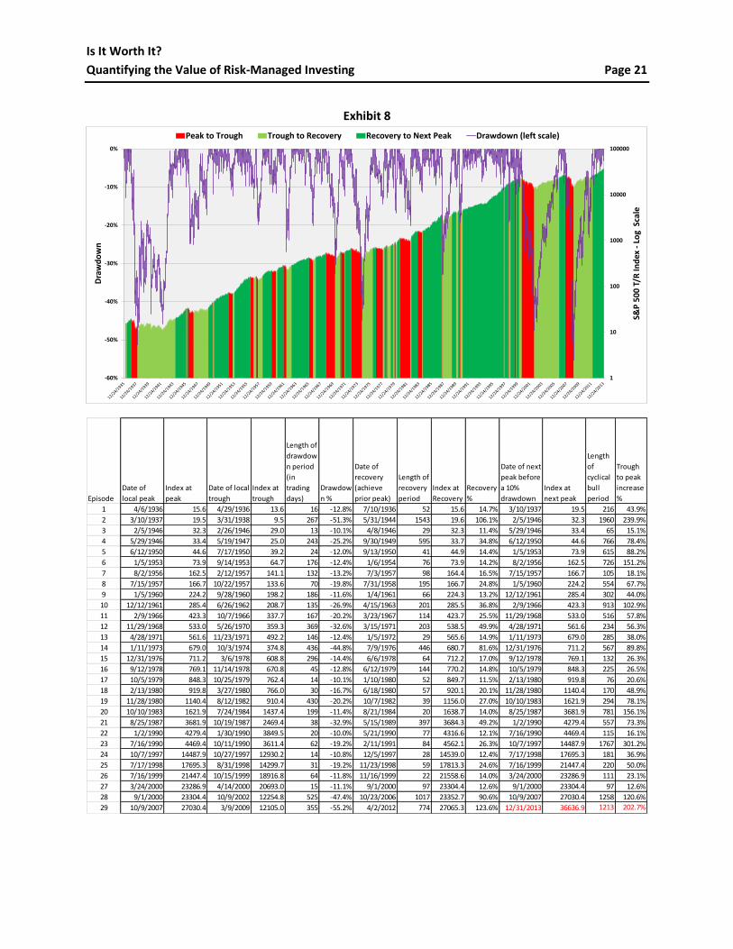
large-cap stocks, as measured by the S&P 500 Total Return Index (see note12). In Exhibit 8,

below, we reproduce the graph we introduced in Exhibit 5, and include below it a table which

contains key information on each of the 29 episodes (shaded red in the graph) during which the

index suffered a drawdown of -10% or worse. Specifically, for each episode, we note the date

of the local peak of the index; the index value at that peak; the date of the subsequent local

trough (i.e., after the -10%-or-worse decline); the index value at that trough; the length of

drawdown (peak-to-trough) period; the percentage drawdown; the date of recovery (when the

index re-achieves its prior peak); the length of that recovery period; the recovery percentage;

the date of the next local peak (i.e., just prior to its beginning its next -10%-or-worse decline);

the index value at that peak; the length of cyclical bull (trough-to-peak) period; and, finally, the

percentage increase during the bull period. Note that the recovery period is a subset of the bull

period (in terms of the graph, the recovery period is shaded light green, and the bull period is

the combined light- and dark-green-shaded sections). Note also that the figures in red at the

end of the table denote that the final bull period is not yet complete — we simply terminated

the series at 12/31/2013.

The detailed table in Exhibit 8 allows the evaluation of any number of RMI strategies; we can

apply a given RMI strategy to each episode separately, calculate its impact, summarize the

results over several episodes, and draw conclusions.

Consistent with the main text, let’s first focus on an RMI strategy that is successful in reducing

the impact of a drawdown by half of its extent beyond -10%, net of the cost of the strategy. For

example, a -30% drawdown would be reduced to -20%, a -20% drawdown would be reduced to

-15%, and a -10% drawdown would be reduced not at all and remain at -10%. In Exhibit 9, we

apply this strategy to each of the 29 episodes. It is a straightforward matter to then calculate

12

Source: Bloomberg

Is It Worth It?


the tolerable performance drag during the subsequent bull period of each episode, such that

the resulting performance over the episode’s full cycle is no worse than would have been the

case without the RMI strategy. These calculations are spelled out in the notes to Exhibit 9.

Column H of the exhibit shows the tolerable performance drag for each episode in isolation.

Since the length of each episode’s full cycle is generally much shorter than a typical investor’s

investment horizon, we show the results of successive rolling-five-episode periods in column I.

From column I, we derive the 25th and 75th percentiles shown in Exhibit 7 of the text.

We performed similar analyses for RMI strategies that provide different levels of protection

(namely, 25% and 75%) of the drawdown below -10%. These calculations are not reproduced

here, but are straightforward versions of those just described, and the results are summarized

in Exhibit 7 of the text.

Note that we have not included an RMI strategy that protects 100% of the downside below -

10%. This is because we believe it is a practical impossibility. While a 10%-out-of-the-money

put option on the S&P 500 Total Return Index may appear to provide such protection, it does

not. To provide true 100% protection against any drawdown worse than -10%, the put strike

would need to be revised upwards each day that the index rises above its prior peak.

Furthermore, any time that the put was exercised (and, to provide true 100% protection, it

would need to be exercised immediately on the day that the index falls -10% from its prior

peak), it would need to be replaced seamlessly with another put, but this put would need be at-

the-money. The chance of needing to exercise that put in the near future is almost a certainty

— at which point it would need to be replaced with another at-the-money-put, and so on.

Aside from being extremely expensive, this method of protection is not feasible as a practical

matter. In contrast, RMI strategies that deliver protection of less than 100% are indeed feasible

— examples include the tail risk hedges described in “Integrated Tail Risk Hedging: The Last Line

of Defense in Investment Risk Management” (see note13).

It may be instructive to graph some key results.

13

Journal of Financial Planning, June 2012

http://www.brintoneaton.com/wp-content/uploads/2012/07/JAM-JFP-June-2012-Tail-Risk-Hedging-00061935.pdf

http://www.brintoneaton.com/wp-content/uploads/2012/07/JAM-JFP-June-2012-Tail-Risk-Hedging-00061935.pdf

Is It Worth It?


In the text (and in Exhibit 6), we estimated that a particular RMI strategy — i.e., one that

reduces equity market declines by half of the excess decline below -10% — adds value as long

as its “cost” (performance drag during bull markets) does not exceed 425 basis points per

annum.

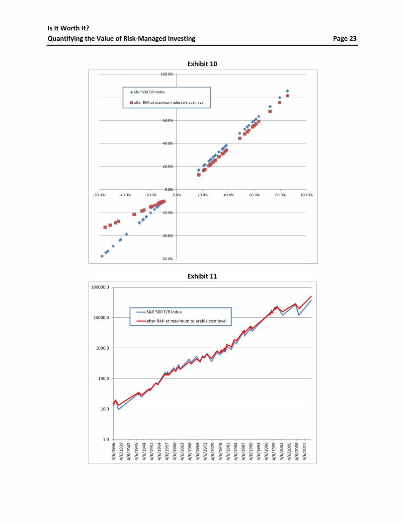
Exhibit 10 shows the “payoff profile” (see note14) of such an RMI strategy whose cost is

precisely 425 basis points. On the left side of the graph, we plot — for each of the 29

drawdowns in our historical record — the net returns of a portfolio with this RMI strategy (in

red), compared to the corresponding returns of the same portfolio without the strategy (in

blue). On the right side of the graph, we plot — for each of the 29 subsequent bull periods —

the annualized returns of the corresponding portfolios.

In our final graph, in Exhibit 11, we show the cumulative performance (on log scale) of the same

two portfolios described immediately above.

14

The “payoff profile” graph is commonly used in visualizing various option strategies (calls, puts, collars, straddles, etc.), and we assume the reader is familiar with its interpretation.

Is It Worth It?


Exhibit 8

1

10

100

1000

10000

100000

-60%

-50%

-40%

-30%

-20%

-10%

0%

S&P

50

0 T

/R In

dex

-Lo

g S

cale

Dra

wd

ow

n

Peak to Trough Trough to Recovery Recovery to Next Peak Drawdown (left scale)

Episode

Date of

local peak

Index at

peak

Date of local

trough

Index at

trough

Length of

drawdow

n period

(in

trading

days)

Drawdow

n %

Date of

recovery

(achieve

prior peak)

Length of

recovery

period

Index at

Recovery

Recovery

%

Date of next

peak before

a 10%

drawdown

Index at

next peak

Length

of

cyclical

bull

period

Trough

to peak

increase

%

1 4/6/1936 15.6 4/29/1936 13.6 16 -12.8% 7/10/1936 52 15.6 14.7% 3/10/1937 19.5 216 43.9%

2 3/10/1937 19.5 3/31/1938 9.5 267 -51.3% 5/31/1944 1543 19.6 106.1% 2/5/1946 32.3 1960 239.9%

3 2/5/1946 32.3 2/26/1946 29.0 13 -10.1% 4/8/1946 29 32.3 11.4% 5/29/1946 33.4 65 15.1%

4 5/29/1946 33.4 5/19/1947 25.0 243 -25.2% 9/30/1949 595 33.7 34.8% 6/12/1950 44.6 766 78.4%

5 6/12/1950 44.6 7/17/1950 39.2 24 -12.0% 9/13/1950 41 44.9 14.4% 1/5/1953 73.9 615 88.2%

6 1/5/1953 73.9 9/14/1953 64.7 176 -12.4% 1/6/1954 76 73.9 14.2% 8/2/1956 162.5 726 151.2%

7 8/2/1956 162.5 2/12/1957 141.1 132 -13.2% 7/3/1957 98 164.4 16.5% 7/15/1957 166.7 105 18.1%

8 7/15/1957 166.7 10/22/1957 133.6 70 -19.8% 7/31/1958 195 166.7 24.8% 1/5/1960 224.2 554 67.7%

9 1/5/1960 224.2 9/28/1960 198.2 186 -11.6% 1/4/1961 66 224.3 13.2% 12/12/1961 285.4 302 44.0%

10 12/12/1961 285.4 6/26/1962 208.7 135 -26.9% 4/15/1963 201 285.5 36.8% 2/9/1966 423.3 913 102.9%

11 2/9/1966 423.3 10/7/1966 337.7 167 -20.2% 3/23/1967 114 423.7 25.5% 11/29/1968 533.0 516 57.8%

12 11/29/1968 533.0 5/26/1970 359.3 369 -32.6% 3/15/1971 203 538.5 49.9% 4/28/1971 561.6 234 56.3%

13 4/28/1971 561.6 11/23/1971 492.2 146 -12.4% 1/5/1972 29 565.6 14.9% 1/11/1973 679.0 285 38.0%

14 1/11/1973 679.0 10/3/1974 374.8 436 -44.8% 7/9/1976 446 680.7 81.6% 12/31/1976 711.2 567 89.8%

15 12/31/1976 711.2 3/6/1978 608.8 296 -14.4% 6/6/1978 64 712.2 17.0% 9/12/1978 769.1 132 26.3%

16 9/12/1978 769.1 11/14/1978 670.8 45 -12.8% 6/12/1979 144 770.2 14.8% 10/5/1979 848.3 225 26.5%

17 10/5/1979 848.3 10/25/1979 762.4 14 -10.1% 1/10/1980 52 849.7 11.5% 2/13/1980 919.8 76 20.6%

18 2/13/1980 919.8 3/27/1980 766.0 30 -16.7% 6/18/1980 57 920.1 20.1% 11/28/1980 1140.4 170 48.9%

19 11/28/1980 1140.4 8/12/1982 910.4 430 -20.2% 10/7/1982 39 1156.0 27.0% 10/10/1983 1621.9 294 78.1%

20 10/10/1983 1621.9 7/24/1984 1437.4 199 -11.4% 8/21/1984 20 1638.7 14.0% 8/25/1987 3681.9 781 156.1%

21 8/25/1987 3681.9 10/19/1987 2469.4 38 -32.9% 5/15/1989 397 3684.3 49.2% 1/2/1990 4279.4 557 73.3%

22 1/2/1990 4279.4 1/30/1990 3849.5 20 -10.0% 5/21/1990 77 4316.6 12.1% 7/16/1990 4469.4 115 16.1%

23 7/16/1990 4469.4 10/11/1990 3611.4 62 -19.2% 2/11/1991 84 4562.1 26.3% 10/7/1997 14487.9 1767 301.2%

24 10/7/1997 14487.9 10/27/1997 12930.2 14 -10.8% 12/5/1997 28 14539.0 12.4% 7/17/1998 17695.3 181 36.9%

25 7/17/1998 17695.3 8/31/1998 14299.7 31 -19.2% 11/23/1998 59 17813.3 24.6% 7/16/1999 21447.4 220 50.0%

26 7/16/1999 21447.4 10/15/1999 18916.8 64 -11.8% 11/16/1999 22 21558.6 14.0% 3/24/2000 23286.9 111 23.1%

27 3/24/2000 23286.9 4/14/2000 20693.0 15 -11.1% 9/1/2000 97 23304.4 12.6% 9/1/2000 23304.4 97 12.6%

28 9/1/2000 23304.4 10/9/2002 12254.8 525 -47.4% 10/23/2006 1017 23352.7 90.6% 10/9/2007 27030.4 1258 120.6%

29 10/9/2007 27030.4 3/9/2009 12105.0 355 -55.2% 4/2/2012 774 27065.3 123.6% 12/31/2013 36636.9 1213 202.7%

Is It Worth It?


Exhibit 9

A B C D E F G H I

Episode

Drawdown

%

Adj'd

Drawdown

%

Trough to

peak

increase %

Adj'd

(breakeven

) trough to

peak

increase %

Length of

cyclical bull

period

Annualized

Trough to

peak

increase %

Annualized

Adj'd

(breakeven

) trough to

peak

increase %

breakeve

n cost in

bps p.a.

rolling 5-

period

avg

1 -12.8% -11.4% 43.9% 41.6% 216 52.4% 49.6% 275

2 -51.3% -30.7% 239.9% 138.6% 1960 16.9% 11.7% 516

3 -10.1% -10.1% 15.1% 15.1% 65 72.0% 71.6% 39

4 -25.2% -17.6% 78.4% 61.9% 766 20.8% 17.0% 376

5 -12.0% -11.0% 88.2% 86.1% 615 29.3% 28.7% 59 253

6 -12.4% -11.2% 151.2% 147.8% 726 37.3% 36.7% 64 211

7 -13.2% -11.6% 18.1% 16.0% 105 48.6% 42.3% 628 233

8 -19.8% -14.9% 67.7% 58.1% 554 26.3% 22.9% 334 292

9 -11.6% -10.8% 44.0% 42.7% 302 35.2% 34.2% 100 237

10 -26.9% -18.4% 102.9% 81.9% 913 21.4% 17.8% 358 297

11 -20.2% -15.1% 57.8% 48.3% 516 24.7% 21.0% 369 358

12 -32.6% -21.3% 56.3% 33.9% 234 61.1% 36.6% 2457 724

13 -12.4% -11.2% 38.0% 36.1% 285 32.6% 31.1% 154 688

14 -44.8% -27.4% 89.8% 44.3% 567 32.6% 17.5% 1510 970

15 -14.4% -12.2% 26.3% 23.2% 132 55.7% 48.4% 731 1044

16 -12.8% -11.4% 26.5% 24.5% 225 29.8% 27.5% 226 1016

17 -10.1% -10.1% 20.6% 20.6% 76 85.4% 84.9% 44 533

18 -16.7% -13.4% 48.9% 43.1% 170 79.5% 69.4% 1014 705

19 -20.2% -15.1% 78.1% 67.5% 294 63.4% 55.0% 835 570

20 -11.4% -10.7% 156.1% 154.2% 781 35.1% 34.8% 33 430

21 -32.9% -21.5% 73.3% 48.0% 557 28.0% 19.2% 875 560

22 -10.0% -10.0% 16.1% 16.1% 115 38.3% 38.3% 7 553

23 -19.2% -14.6% 301.2% 279.6% 1767 21.7% 20.8% 95 369

24 -10.8% -10.4% 36.9% 36.3% 181 54.2% 53.3% 89 220

25 -19.2% -14.6% 50.0% 41.9% 220 58.5% 48.9% 965 406

26 -11.8% -10.9% 23.1% 21.9% 111 59.7% 56.1% 361 304

27 -11.1% -10.6% 12.6% 11.9% 97 35.8% 33.6% 222 346

28 -47.4% -28.7% 120.6% 62.7% 1258 17.0% 10.2% 687 465

29 -55.2% -32.6% 202.7% 101.1% 1213 25.6% 15.5% 1015 650

Notes to Exhibit 9:

Columns A, C, and E are from Exhibit 8

Column B is derived by applying the RMI strategy to column A

Column D is calculated as (using Excel notation): (1+C)*((1+A)/(1+B))-1

Columns F and G are annualized versions of columns C and D, respectively. E.g., column F is

calculated as: (1+C)^(250/E), since there are approx. 250 trading days per annum

Column H is the difference between columns F and G, expressed in terms of basis points

per annum

Column I is the rolling-five-episode average of column H

Is It Worth It?


Exhibit 10

Exhibit 11

-60.0%

-40.0%

-20.0%

0.0%

20.0%

40.0%

60.0%

80.0%

100.0%

-60.0% -40.0% -20.0% 0.0% 20.0% 40.0% 60.0% 80.0% 100.0%

S&P 500 T/R Index

after RMI at maximum tolerable cost level

1.0

10.0

100.0

1000.0

10000.0

100000.0

4/6

/19

36

4/6

/19

39

4/6

/19

42

4/6

/19

45

4/6

/19

48

4/6

/19

51

4/6

/19

54

4/6

/19

57

4/6

/19

60

4/6

/19

63

4/6

/19

66

4/6

/19

69

4/6

/19

72

4/6

/19

75

4/6

/19

78

4/6

/19

81

4/6

/19

84

4/6

/19

87

4/6

/19

90

4/6

/19

93

4/6

/19

96

4/6

/19

99

4/6

/20

02

4/6

/20

05

4/6

/20

08

4/6

/20

11

S&P 500 T/R Index

after RMI at maximum tolerable cost level

Is It Worth It?


This whitepaper is limited to the dissemination of general information pertaining to investment services and general

economic market conditions. The information contained herein should not be construed as personalized investment

advice and should not be considered as a solicitation to buy or sell any security or engage in a particular investment

strategy. The views expressed are for commentary purposes only and do not take into account any individual

personal, financial, or tax considerations. There is no guarantee that the views and opinions expressed in this

whitepaper will come to pass. There are risks involved with investing, including the possible loss of principal that

investors should be prepared to bear. Past performance does not guarantee future results.

This material represents an assessment of the market environment at a specific point in time, is subject to change

without notice, and should not be relied upon by the reader as research or investment advice. With regard to sources

of information, certain of the economic and market information contained herein has been obtained from published

sources and/or prepared by third parties. While such sources are believed to be reliable, Giralda Advisors, LLC,

(“Giralda”) or their respective affiliates, employees, or representatives do not assume any responsibility for the

accuracy of such information.

Giralda is an SEC registered investment adviser with its principal place of business in the State of New Jersey.

Giralda and its representatives are in compliance with the current registration and notice filing requirements imposed

upon registered investment advisers by those states in which such registration or notice filing is required. Giralda

may only transact business in those states in which it is notice filed, or qualifies for an exemption or exclusion from

notice filing requirements. Any subsequent, direct communication by Giralda with a prospective client shall be

conducted by a representative that is either registered or qualifies for an exemption or exclusion from registration in

the state where the prospective client resides. For additional information about Giralda, including fees and services,

send for our disclosure statement as set forth on Form ADV using the contact information herein or refer to the

Investment Adviser Public Disclosure web site (www.adviserinfo sec.gov). Please read the Disclosure Brochure

carefully before you invest or send money.

is it worth it? quantifying the value of risk-managed · pdf fileis it worth it? quantifying...

Documents