is-lm model model.pdflm curve to the right, ... is-lm model takes into account the fall in private...

IS-LM Model

1

IS-LM model: Hicks and Hansen

Integration of the real and money markets

Department of Economics and Foundation Course, R.A.P.C.C.E.

2

The Derivation of the IS Curve:

The aggregate demand is determined by consumption

demand and investment demand. Thus IS curve relates

different equilibrium levels of national income with

various rates of interest.

With a fall in the rate of interest, the planned investment

will increase which will cause an upward shift in

aggregate demand function resulting in goods market

equilibrium at a higher level of national income. Department of Economics and Foundation Course, R.A.P.C.C.E.

Goods Market Equilibrium-

3


Derivation of IS Curve

4


Derivation of IS Curve

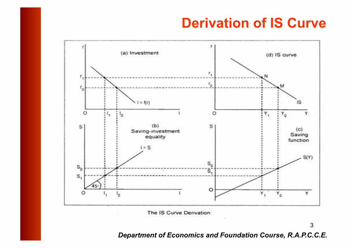
The derivation of IS curve can be made in terms of a

four-part diagram.

In part (a), we have drawn investment function that

shows the inverse relationship between investment

and the rate of interest.

Part (c) plots the saving function that represents direct

relationship between income and saving.

Part (b) is simply a 45° identity line, and

part (d) plots the IS curve.

5

Slope of IS Curve- IS curve is negatively sloped. This is because increase

in interest rate causes investment spending to rise

which shifts the aggregate demand curve up and raises

the equilibrium income level. Also, increase in interest

rate causes investment to fall, which shifts aggregate

demand curve down and lowers the equilibrium income

level.

Department of Economics and Foundation Course, R.A.P.C.C.E

IS Curve

6

Shifts in IS curve-

Changes in factors apart from interest rate that would

shift the aggregate demand would shift the IS curve.

E.g. Increase in autonomous investment will shift the IS

curve to the right , while decrease in autonomous

investment will shift the IS curve to the left.


IS Curve

7


Derivation of LM Curve-

The demand for money is a demand for real balances

because people hold money for what it will buy. The

demand for real balances depends on real income

and rate of interest.

Money Market Equilibrium-

8

LM Curve-

9

Derivation of LM Curve

A four-part diagram may be used to derive the LM curve.

In above Fig. part(a) shows a proportional relationship

between money income and transaction demand for

money (Mt= kPY).

Part (c) represents speculative demand for money [MS =

f(r)].

The schedule in (b) is an identity line that mechanically

divides money supply into transaction and speculative

elements.

Part (d) represents the LM curve.

10

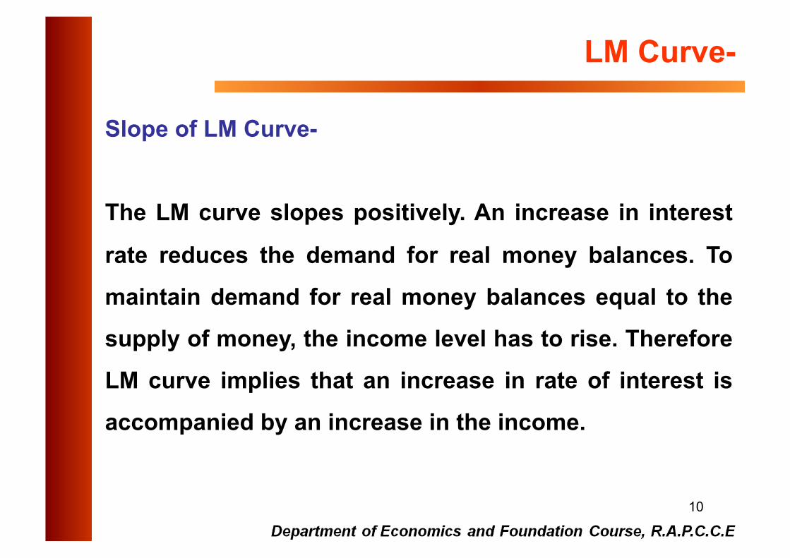
Slope of LM Curve-

The LM curve slopes positively. An increase in interest

rate reduces the demand for real money balances. To

maintain demand for real money balances equal to the

supply of money, the income level has to rise. Therefore

LM curve implies that an increase in rate of interest is

accompanied by an increase in the income.

LM Curve-

11

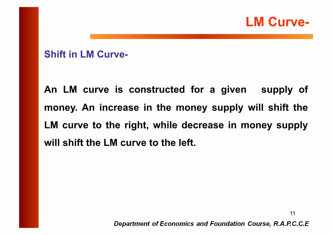
Shift in LM Curve-

An LM curve is constructed for a given supply of

money. An increase in the money supply will shift the

LM curve to the right, while decrease in money supply

will shift the LM curve to the left.

LM Curve-

12

Equilibrium of the IS-LM curve-

13

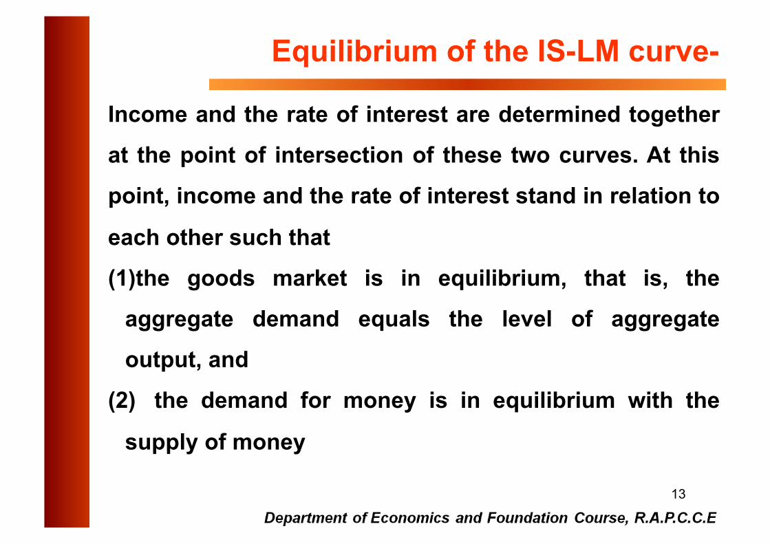
Equilibrium of the IS-LM curve-

Income and the rate of interest are determined together

at the point of intersection of these two curves. At this

point, income and the rate of interest stand in relation to

each other such that

(1) the goods market is in equilibrium, that is, the

aggregate demand equals the level of aggregate

output, and

(2)  the demand for money is in equilibrium with the

supply of money

14

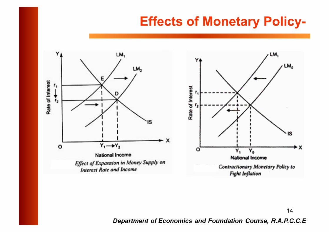
Effects of Monetary Policy-

15

IS-LM model can be used to show the effect of

expansionary and tight monetary policies.

A change in money supply causes a shift in the LM

curve

Expansion in money supply shifts it to the right and

decrease in money supply shifts it to the left.

Effects of Monetary Policy-

16

Effects of Fiscal Policy-

17

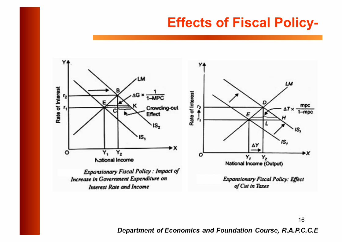
Increase in Government expenditure which is of

autonomous nature raises aggregate demand for goods

and services and thereby causes an outward shift in IS

curve which increases the rate of interest.

IS-LM model takes into account the fall in private

investment due to the rise in interest rate that takes

place with the increase in Government expenditure.


18

That is, increase in Government expenditure crowds out

some private investment.

An alternative measure of expansionary fiscal policy

that may be adopted is the reduction in taxes which

through increase in disposable income of the people

raises consumption demand of the people. As a result,

cut in taxes causes a shift in the IS curve to the right.


is-lm model model.pdflm curve to the right, ... is-lm model takes into account the fall in private...

Documents