is the franc zone an optimal currency area?

Is the Franc Zone an Optimal Currency Area?*

by

David Fielding

Kalvinder Shields

Department of Economics,

University of Leicester**

First Draft: October 1999

Abstract

In this paper we modify the method of Blanchard and Quah (1989) in order to estimate a

structural VAR model appropriate for a small open economy. In this way we identify shocks

to output and prices in the members of the two monetary unions that make up the African

CFA Franc Zone. The costs of monetary union membership will depend on the extent to

which price and output shocks are correlated across countries, and the degree of similarity in

the long run effects of the shocks on the macro-economy. The policy conclusions depend on

the relative importance of different macroeconomic variables to policymakers, and the speed

with which a policymaker is able to respond to a shock.

JEL categories: O11, O23, F33, F42

Keywords: Franc Zone, Optimal Currency Areas, Structural VAR Models

* We are grateful to Kevin Lee, David Vines and seminar participants at the Centre for the Study of African

Economies, University of Oxford for helpful comments and advice; all errors are our own.

** Address for correspondence: Dr Kalvinder Shields, Department of Economics, University of Leicester,

University Road, Leicester LE1 7RH; tel. +44-116-252-5368; fax +44-116-252-2908; e-mail [email protected].

2

1. Introduction

The 1990s have seen a growing interest in the adoption of “hard fixed” exchange rates in

LDCs as a possible way of making a credible commitment to a low domestic inflation rate

(Edwards, 1993). An irrevocable commitment to a fixed exchange rate may help to solve the

time inconsistency problems raised in Kydland and Prescott (1977) and Barro and Gordon

(1983); it may also prevent self-fulfilling currency crises (Davies and Vines, 1995). Recent

research indicates that countries that have made a realistic commitment to a fixed exchange

rate policy do have lower average inflation rates (Ghosh et al., 1995; Anyadike-Danes, 1995;

Fielding and Bleaney, 1999). The realism of the commitment depends on the institutional

framework within which the exchange rate is fixed. In the recent past the most successful

unilateral attempts to adhere to a fixed exchange rate have involved the introduction of

currency boards, as for example in Argentina or Estonia. This has led to a renewed interest in

currency boards as a stabilization tool (Bennett, 1992; Schwartz, 1993; Hanke, 1996; Balino

et al., 1997; Gulde, 1997; Ghosh et al., 1998; Edwards, 1999).

The credibility of commitment that comes with a currency board results from that fact

that any devaluation is impossible without destroying the whole system. However, there are

alternative ways of gaining credibility. In Africa the CFA Franc Zone consists of two monetary

unions between different African states. The two CFA currencies have been pegged to the

French Franc (and now the ECU1) since 1948, with the French treasury guaranteeing to

exchange French currency for CFA currency at a fixed rate (Vizy, 1989). This rate can be

adjusted for either of the two monetary unions, but only by the mutual consent of all the

members of the union and France. In fact, the rate has been adjusted only once, in January 1994.

The system preserves some flexibility with the option of devaluation in extremis: joining the

CFA is not tantamount to ECU-ization. The credibility of the peg comes from the fact that such

a devaluation is never a unilateral option, and can only be achieved by the unanimous agreement

of the partner countries.

The disadvantage of Franc Zone membership is that there can only be a single

monetary policy in each monetary union. Suppose that two countries experience

heterogeneous shocks (by “shocks” we mean those innovations in macroeconomic variables

that are not induced by changes in policy). The only country-specific response available to

their governments is through fiscal policy; but in francophone Africa fiscal instruments are

1 The fixed exchange rate is a budgetary agreement between France and its former colonies, so France’s membership of the EMU has not prejudiced the system (Hadjimichael and Galy, 1997).

3

often too unwieldy for them to be used as stabilization tools (Chambas, 1994). So CFA

members commit themselves to stabilization policy that is determined by some cross-country

aggregate welfare function, a policy that may differ sharply from the optimal policy for any

one individual country.2

In this paper we will not attempt to answer the grand question of whether, for each

member of the CFA, the benefits of low inflation outweigh the costs of giving up monetary

independence. But we will do some groundwork for an answer to this question by looking in

more detail at the nature of the shocks experienced by Franc Zone countries. We will estimate

the degree of cross-country correlation between shocks to different macroeconomic variables,

and look at the degree of similarity in the effect these shocks eventually have on the economy.

1.1 The current composition of the Franc Zone

The two CFA monetary unions are the West African Economic and Monetary Union (UEMOA)

and the region of the Central Bank of Equatorial Africa (BEAC). The countries that will appear

in this paper are Benin (denoted in the tables below as ben), Burkina Faso (bfa), Cote d’Ivoire

(civ), Senegal (sen), Togo (tgo), Mali (mli) and Niger (ner) – all UEMOA members - plus

Cameroon (cmr), Congo Republic (cgo), Gabon (gab), Centrafrique (car) and Chad (tcd) – all

BEAC members. There are two recent additions to the CFA missing from our paper because of

inadequate data: Equatorial Guinea and Guinea-Bissau. With the exception of these two

countries, the members of the CFA were all part of the French Empire in Africa, and the

division between the UEMOA and the BEAC region corresponds to an imperial administrative

division.

For the current structure of the CFA to be optimal the degree of similarity within each

monetary union ought to be at least as great as the degree of similarity between any one

country and the countries of the other monetary union. Otherwise, it would reduce the costs of

monetary union membership to redraw the boundaries between the two unions. The two

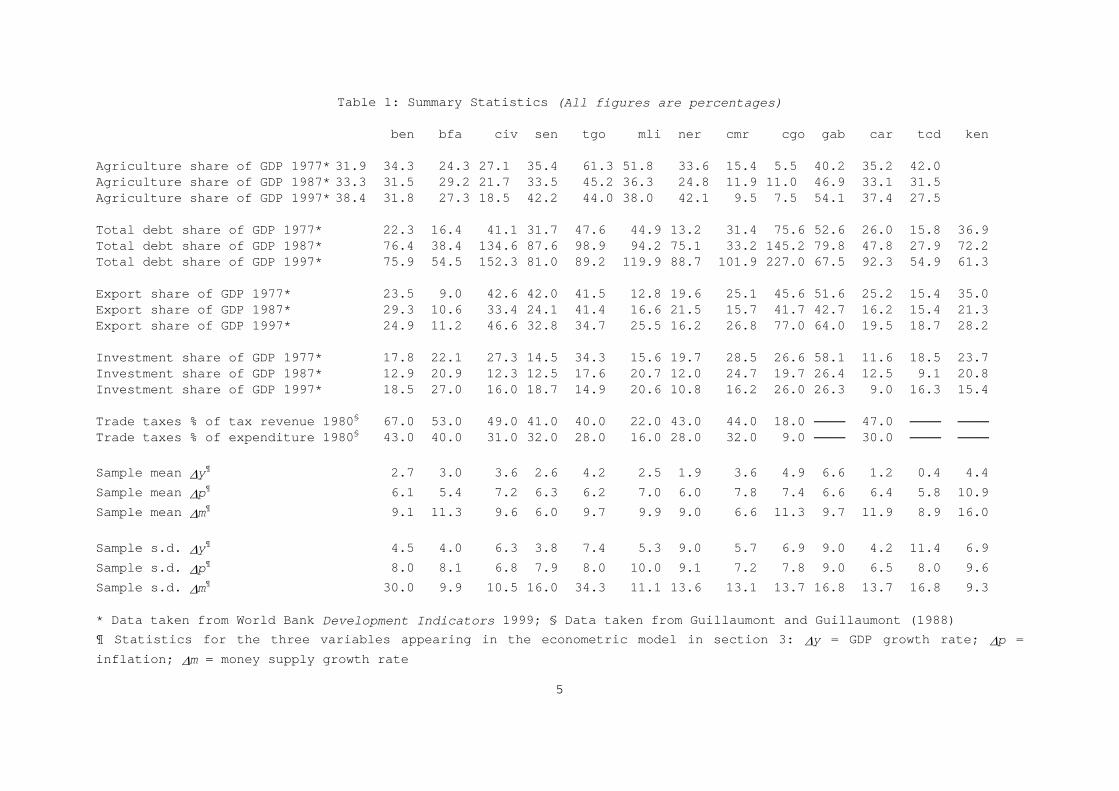
existing groups of countries, bound together largely by historical accident, embody a wide

variety of economic structures, as illustrated in Table 1. The BEAC region includes three

petroleum exporters (Cameroon, Congo Republic and Gabon) alongside three very poor

countries exporting cash crops (Centrafrique, Chad and Equatorial Guinea). The UEMOA

2 The form of the social welfare function will depend on the voting or lobbying power of each country in the Adminstrative Council of each central bank. In the UEMOA central bank each member state plus France has two votes, regardless of their relative size. In the BEAC Cameroon has four votes, France three, Gabon two and the other member states one. In both unions the weights given to the interests of each African country are unlikely

4

includes two relatively large economies (Cote d’Ivoire and Senegal) alongside six much

smaller ones. Within this region there is some cross-border labour mobility, notably

migration between Mali and Cote d’Ivoire, and to a lesser extent between Burkina Faso /

Togo and Cote d’Ivoire. But Senegal and Guinea-Bissau are separated from their partner

countries by the desert of western Mali, across which there is relatively little movement of

labour.3 It would be a very happy accident if the current partitioning of the Franc Zone turned

out to be optimal.

A related question is whether there is a greater degree of similarity of shocks within

the Franc Zone than there is between the Franc Zone and the rest of Africa. If it turns out that

there is not, then the case for an exclusively francophone monetary area is much weaker. The

monetary stability of the CFA is a positive externality generated by the European Monetary

Union, which could in principle be extended to anglophone African countries. This question

is difficult to answer because the nature of the shocks experienced by Franc Zone countries

may partly be a consequence of their monetary and exchange rate system. Even if one controls

for quantitative measures of monetary policy (as we intend to do), it is unlikely that the

shocks experienced by a country with a floating exchange rate or a crawling peg will be the

same as those experienced by a CFA country, ceteris paribus. There are not that many

anglophone countries for which adequate macroeconomic data are available and which have

maintained a fixed currency peg for any length of time, and with which one might therefore

compare the CFA countries. In this paper we will compare shocks to the Franc Zone with

shocks to Kenya, a coffee exporter with an economic structure similar to, for example, Cote

d’Ivoire and with an historical inflation rate low by anglophone African standards (see Table

1). However, the comparison must be interpreted with a large caveat: Kenya’s financial

system is not the same as that of the CFA, and for long periods its currency peg was

maintained at the expense of foreign exchange rationing (Adam, 1992).

1.2 Measuring and interpreting shocks

The aim of this paper is to identify and compare macroeconomic shocks to different members of the CFA, and to Kenya. We will focus on shocks to aggregate output growth and to aggregate consumer price inflation, which are the two variables that appear most often in analyses of the potential cost and benefits of CFA membership (Devarajan, 1991). We will

to be uniform, but neither are the weights given to the interests of the smaller countries likely to be zero.

5

Table 1: Summary Statistics (All figures are percentages)

ben bfa civ sen tgo mli ner cmr cgo gab car tcd ken

Agriculture share of GDP 1977* 31.9 34.3 24.3 27.1 35.4 61.3 51.8 33.6 15.4 5.5 40.2 35.2 42.0 Agriculture share of GDP 1987* 33.3 31.5 29.2 21.7 33.5 45.2 36.3 24.8 11.9 11.0 46.9 33.1 31.5 Agriculture share of GDP 1997* 38.4 31.8 27.3 18.5 42.2 44.0 38.0 42.1 9.5 7.5 54.1 37.4 27.5

Total debt share of GDP 1977* 22.3 16.4 41.1 31.7 47.6 44.9 13.2 31.4 75.6 52.6 26.0 15.8 36.9 Total debt share of GDP 1987* 76.4 38.4 134.6 87.6 98.9 94.2 75.1 33.2 145.2 79.8 47.8 27.9 72.2 Total debt share of GDP 1997* 75.9 54.5 152.3 81.0 89.2 119.9 88.7 101.9 227.0 67.5 92.3 54.9 61.3

Export share of GDP 1977* 23.5 9.0 42.6 42.0 41.5 12.8 19.6 25.1 45.6 51.6 25.2 15.4 35.0 Export share of GDP 1987* 29.3 10.6 33.4 24.1 41.4 16.6 21.5 15.7 41.7 42.7 16.2 15.4 21.3 Export share of GDP 1997* 24.9 11.2 46.6 32.8 34.7 25.5 16.2 26.8 77.0 64.0 19.5 18.7 28.2

Investment share of GDP 1977* 17.8 22.1 27.3 14.5 34.3 15.6 19.7 28.5 26.6 58.1 11.6 18.5 23.7 Investment share of GDP 1987* 12.9 20.9 12.3 12.5 17.6 20.7 12.0 24.7 19.7 26.4 12.5 9.1 20.8 Investment share of GDP 1997* 18.5 27.0 16.0 18.7 14.9 20.6 10.8 16.2 26.0 26.3 9.0 16.3 15.4

Trade taxes % of tax revenue 1980§ 67.0 53.0 49.0 41.0 40.0 22.0 43.0 44.0 18.0 47.0 Trade taxes % of expenditure 1980§ 43.0 40.0 31.0 32.0 28.0 16.0 28.0 32.0 9.0 30.0

Sample mean ∆y¶ 2.7 3.0 3.6 2.6 4.2 2.5 1.9 3.6 4.9 6.6 1.2 0.4 4.4 Sample mean ∆p¶ 6.1 5.4 7.2 6.3 6.2 7.0 6.0 7.8 7.4 6.6 6.4 5.8 10.9 Sample mean ∆m¶ 9.1 11.3 9.6 6.0 9.7 9.9 9.0 6.6 11.3 9.7 11.9 8.9 16.0

Sample s.d. ∆y¶ 4.5 4.0 6.3 3.8 7.4 5.3 9.0 5.7 6.9 9.0 4.2 11.4 6.9 Sample s.d. ∆p¶ 8.0 8.1 6.8 7.9 8.0 10.0 9.1 7.2 7.8 9.0 6.5 8.0 9.6 Sample s.d. ∆m¶ 30.0 9.9 10.5 16.0 34.3 11.1 13.6 13.1 13.7 16.8 13.7 16.8 9.3

* Data taken from World Bank Development Indicators 1999; § Data taken from Guillaumont and Guillaumont (1988) ¶ Statistics for the three variables appearing in the econometric model in section 3: ∆y = GDP growth rate; ∆p = inflation; ∆m = money supply growth rate

6

assume nothing about the relative weights ascribed to hitting output and inflation targets: any

policy conclusions drawn from the comparison of output and inflation shocks are conditional on

the weights in the policymaker’s social welfare function.

We will also be agnostic about the speed with which a monetary policy response to a

shock is feasible. If an immediate response is possible then the prime concern will be the

degree of similarity in the shocks hitting the economy (and therefore the degree of similarity

in the monetary policy response most appropriate for each country), regardless of the degree

of similarity in their consequent long run effects. When the policymaker can neutralize any

shocks with a timely policy response their potential long run effects are not a prime concern.

But if an immediate response is not possible then the long run effects are as important as the

characteristics of the initial shocks, so we will look at both.

Many existing papers on the identification and cross-country comparison of

macroeconomic shocks follow the method of Blanchard and Quah (1989). Examples are

Bayoumi and Eichengreen (1994, 1996) and Funke (1995). This involves estimating a

reduced form VAR for inflation and output growth, and identifying structural shocks to each

variable by imposing a set of restrictions that includes the theory-based assumption that in the

long run output shocks can affect inflation but not vice versa. We will adopt the general

modelling strategy of Blanchard and Quah in this paper, but within the framework of a

different theoretical model. We do not assume that output growth is independent of inflation

in the long run, because there is evidence from empirical work on growth and investment in

LDCs that high inflation can have deleterious consequences for long run growth (Fischer,

1993).4 This could be either because high inflation is associated with a higher degree of price

uncertainty, depressing investment (as in, for example, Green and Villanueva, 1990), or because

larger and more frequent price changes increase search costs. Moreover, the motivation for the

paper comes from the identification of those country-specific shocks that are not the result of

innovations in monetary policy. So we need to identify shocks to output growth and inflation

conditional on money supply growth in the CFA and Kenya and on common foreign price

shocks. For this reason, our VAR will include four variables, not two. The theoretical model

that provides the identifying restrictions in this VAR will be described in the next section; this

will be followed by a discussion of the econometric modeling framework. Section 3 presents

and interprets the econometric results, and Section 4 concludes.

4 Bruno and Easterly (1998) contest the link between inflation and long run growth. But in the face of conflicting evidence, we choose not to impose the a priori restriction that inflation has no impact on long run growth.

7

2. The Modeling Framework

Our aim is to construct a structural VAR representation of the macro-economy of each member

of the CFA for which data is available, plus Kenya. The estimated innovations in this VAR will

be interpreted as macroeconomic shocks. Inference about the degree of similarity between the

shocks to two countries will be based on the magnitude of the correlation of the innovations in

their respective VARs, and on the degree of similarity in the impact of these innovations on the

rest of the economy. We will focus particularly on shocks to domestic prices and output,

conditional on domestic monetary policy and common foreign price shocks. So the VAR needs

to include domestic money and foreign prices alongside domestic prices and output. The

structural model will be estimated by imposing exactly identifying restrictions on a reduced

form VAR. These restrictions will be imposed on the long run equilibrium in the model, in the

style of Blanchard and Quah (1989), not on short run coefficients. However, the macroeconomic

model we employ is larger than the one used in the traditional Blanchard-Quah framework, and

the restrictions embodied in it have a different theoretical motivation. We begin with a

description of the theory, and then relate this to the econometric model to be estimated in the

following section.

2.1 The theoretical framework

The theoretical model from which the restrictions are derived is a description of the

macroeconomic steady state. The dependent variables in the model are ∆r (real interest rate

growth) ∆m (nominal money stock growth) ∆y (income growth) and ∆p (inflation in domestic

consumer prices). There is one independent variable, ∆pfr (foreign consumer price inflation

times the rate of nominal exchange rate depreciation). In the steady state, the dependent

variables in each economy are determined as follows:5

∆[m - p] = a0 + a1⋅∆y, + a2⋅∆r, a1 ≥ 0 ≥ a2 Money Demand (1)

∆p = b0 + b1⋅∆pfr, b1 ≥ 0 Relative PPP (2)

∆y = c0 + c1⋅∆p + c2⋅∆r, c1 ≤ 0, c2 ≤ 0 Aggregate Supply (3)

5 There is no uncovered interest parity condition in the model. I.e., capital does not flow freely across the borders of the Franc Zone. See Vizy (1989) for a discussion of the institutional restrictions on capital movement between France and the CFA (including multiple taxes on such transfers), and Fielding (1993) for evidence on the absence of interest parity between the CFA and France.

8

∆r = f0 + f1⋅∆y + f2⋅∆[pfr - p], f1≤ 0 ≤ f2 Aggregate Demand (4)

Equation (1) states that long run real money demand growth (with a reasonably wide definition

of money) is a function of real income growth and real interest rate changes. In the steady state,

the nominal money stock is assumed to adjust to clear the money market for a given level of

nominal money demand, and the monetary authorities do not restrict the formation of bank

deposits. There is some evidence for this assumption in Lowrey (1995).

Equation (2) embodies a weak version of the assumption of relative PPP. We do not

assume that domestic and foreign consumer price inflation rates converge in the long run

(although this is possible, if b0 = [1 - b1] = 0). Rather, we assume that if there is any

divergence, it is at least at a constant rate. Lowrey (1995) provides some evidence for this weak

form of relative PPP amongst CFA members, whereas Nuven (1994) is able to reject the

hypothesis of strong PPP for most Franc Zone countries.

Equation (3) allows the growth of aggregate supply to depend on the growth of

aggregate domestic prices, even in the long run. The introduction of the term c1⋅∆p is not

intended to suggest that there is long run money illusion, or that nominal wages are permanently

rigid. Rather, it allows for the possibility that high inflation can have deleterious consequences

for long run growth, as discussed in section 1.2. The coefficient c2 allows interest rate increases

to depress capital stock growth and hence income growth in the long run.

Equation (4) is an inverted aggregate demand curve, in which the growth of aggregate

demand depends on the growth of the interest rate (which will affect domestic demand for

consumption and investment goods) and real exchange rate appreciation (which will affect net

export growth).

The one dependent variable which is difficult to measure in the CFA is the interest rate,

r. The only rate reported consistently throughout the sample period is the official central bank

discount rate, which is unlikely to equal the marginal cost of loanable funds. So we do not

attempt to model ∆r, and instead express equations (3-4) in reduced form:

∆y = [c0 + c2⋅f0 + (c1 - c2⋅f1)⋅∆p + c2⋅f2⋅∆pfr]/[1 - c2⋅f1] (5)

Since c2⋅f1 ≥ 0, the denominator of this expression, and therefore the impact of increases in ∆p

and ∆pfr on ∆y, are ambiguous. For the same reason the term [c1 - c2⋅f1] is ambiguously signed,

9

but c2⋅f2 ≤ 0; so the effects on ∆p and ∆pfr on ∆y could work in the same or in opposite

directions. The “normal” case is when an increase in inflation decreases output growth,

because of its efficiency-reducing effects. However, there is also a “perverse” case when both

the elasticity of aggregate supply with respect to the interest rate and the slope of the IS curve

are greater than unity (c2⋅f1 > 1), so the response of long run growth to inflation flips sign.

Since equation (5) is constructed by substituting the aggregate demand curve into the

aggregate supply curve, the shocks to output in our model are not to be interpreted as “aggregate

demand” or “aggregate supply” shocks. They are more readily interpreted as aggregate “real” (as

opposed to price or nominal money) shocks.

Our equation for money demand growth is also expressed in reduced form:

∆m = a0 + a2⋅f0 + [a1 + a2⋅f1]⋅∆y + a2⋅f2⋅∆pfr + [1 - a2⋅f2]⋅ ∆p (6)

Implicit in equations (5-6) is the equilibrium adjustment of the real marginal cost of loanable

funds. At times both the two central banks of the CFA area and the Central Bank of Kenya have

controlled nominal lending rates on certain types of loan, so it would be very heroic to assume

the equilibrium adjustment of the formal financial sector loan rate. We are rather relying on the

assumption that if the formal sector loans market does not clear, there is at the margin a flexible

curb market interest rate that adjusts endogenously.

The steady state for each economy is described by the values of the parameters in

equations (2) and (5-6) plus a statement of the long run level of ∆pfr:

∆pfr = ∆pfr0 (7)

With a fixed / managed nominal exchange rate ∆pfr is independent of the other variables in the

model.

If we estimate the dynamics of the four variables (∆pfr, ∆p, ∆y, ∆m) within a VAR

framework for which equations (2) and (5-7) describe the steady-state, then there are six long

run restrictions to be imposed. These are the absence of ∆m in equation (5); the absence of ∆y

and ∆m in equation (2); and the absence of ∆p, ∆y and ∆m in equation (7).6 These six

restrictions will be used to identify the system. Note that in this model of a fixed exchange rate

6 There will also be short run restrictions on the equation for ∆pfr, since this variable is strictly exogenous to the other three.

10

economy with relative PPP in the long run, and with a long run aggregate supply function that

includes inflation, shocks to inflation will have a long run impact on output, but shocks to

output will have no impact on inflation. In this way we differ from other papers that use long

run restrictions to identify a macroeconomic model, in which output shocks typically have a

long run impact on inflation, but inflation shocks have no impact on output.

We do not impose corresponding short run restrictions on equations (2) and (5). We

allow changes in ∆m to influence ∆y in the short run, because a disequilibrium in the money

market might well affect aggregate demand, as consumers respond to excess supply of or

demand for money by increasing or reducing their spending. We also allow changes in ∆m and

∆y to affect ∆p in the short run because short run deviations from PPP are possible, and in the

short run prices rather than nominal money may adjust to clear the money market in response to

changes in ∆y or ∆m.

There is no long run restriction on the money growth equation, equation (6). We are

assuming that in the long run, the nominal value of bank deposits can adjust to satisfy people’s

demand, and that this demand depends on inflation, income and the interest rate. In the short

run, when PPP does not have to hold, it may be that money market equilibrium is achieved (at

least partially) by the adjustment of domestic prices. In this case, a shock to the money base

could impact on ∆m in the short run. This does not mean that ∆m can be assumed to be weakly

exogenous to ∆p and ∆y. Central bank decisions about narrow money creation are likely to

depend on the current state of the macro-economy: there is evidence for this with respect to

Cote d’Ivoire and Kenya in Fielding (1999). ∆m is likely to depend on ∆p and ∆y in both the

short run and the long run, but for different reasons.

In the absence of any short run restrictions in our model (except for the strict exogeneity

of ∆pfr) the dynamics of inflation, output growth and money growth can be described by a

system of the form:

B11(L) ∆pfrt = ε1t (7a)

B21(L) ∆pfrt + B22(L) ∆pt + B23(L) ∆yt + B24(L) ∆mt = ε2t (2a)


11


where equation (xa) corresponds to equation (x) above, the Bij(L) are lag polynomials

embodying restrictions to ensure that equations (2) and (5-7) hold in the long run, and the εit are

orthogonal shocks to foreign inflation, domestic inflation, output growth and money growth

respectively. The output growth shocks ε3t combine shocks to aggregate demand with shocks to

aggregate supply, separate identification of the two components being impossible in the absence

of appropriate interest rate data. To the extent that ε3t is dominated by productivity shocks, we

might expect economies with similar production structures to have a relatively high correlation

in ε3t. In the context of the Franc Zone such a group might be formed by the petroleum exporters

(Cameroon, Congo Republic and Gabon) versus the petroleum importers (the rest); or by the

semi-arid Sahelian economies (Burkina Faso, Senegal, Mali, Niger and Chad) versus the other

countries with more tropical climates. But it is also possible that that ε3t is dominated by

aggregate demand shocks. In the absence of any obvious differences in the structure of private

sector demand across the CFA, the most likely reason for differences or similarities in aggregate

demand shocks among Franc Zone members is government behavior. CFA governments differ

in the extent to which their budget deficit is subject to large shocks, because some rely on a

much narrower tax base than others (Bergougnoux, 1988; Chambas, 1994). A government that

is less reliant on import duties or export taxes to finance its expenditure is less likely to have a

highly variable deficit, or at least its deficit is less likely to vary with the international prices of

primary commodities. In Table 1 Congo Republic and Mali stand out from the rest in this

regard. However, if a government is prepared to make use of external borrowing in order to

cushion the domestic economy from shocks to its deficit, such shocks need not translate into

aggregate demand shocks. So governments which have relied on a relatively large amount of

deficit financing and so become highly indebted may differ from the rest. As indicated in Table

1, Congo Republic, Mali and Cote d’Ivoire have the highest debt levels.

2.2 The econometric framework

The identification of the system is based on the methodological framework introduced by

Blanchard and Quah (1989), although our macroeconomic model differs from theirs. For each

country we estimate a reduced form VAR:

12

Xt = A(L)Xt-1 + et = (I – A(L))-1et (8)

where A(L) is a 4 x 4 matrix of lag polynomials and Xt denotes the 4 x 1 vector of stationary

variables:

Xt = [∆pfrt, ∆pt, ∆yt, ∆mt]’ (9)

and we impose the restriction that A12, A13 and A14 = 0, i.e., ∆pfr is strictly exogenous. This four-

variable model corresponds to the system represented by equations (2) and (5-7) above.

Appendix 1 presents evidence that the variables we are dealing with are stationary. et represents

the vector of reduced form residuals. We impose no a priori restrictions on the reduced form

residual covariance matrix. Moreover, the et are likely to be correlated across countries, so all

the VARs must be estimated simultaneously.

In the absence of any theoretical restrictions the reduced form innovations et have no

obvious economic interpretation. Such an interpretation will depend on the derivation of an

alternative moving average representation to equation (8), which formulates variable

movements as a function of past structural shocks, εt:

Xt = C(L)εt (10)

where, in terms of the theoretical model represented by equations (2a) and (5a-7a), C = B-1 and

the matrix εt contains the structural shocks to each equation in the system. The elements of εt are

mutually uncorrelated. This will allow us to estimate the cross-country correlation coefficients

for each element of εt. Moving from equation (8) to equation (10) requires the identification of a

non-singular matrix S that links the reduced form and structural innovations, i.e.:

et = Sεt (11)

where, in terms of equation (10), S = C(0). In an n-variable model identification requires n2

restrictions: in our case, n2 = 16. Following the Blanchard-Quah framework, we assume that the

structural shocks are orthogonal and have unit variance, i.e. Var(εt) = I. This gives us (n+1)n/2 =

13

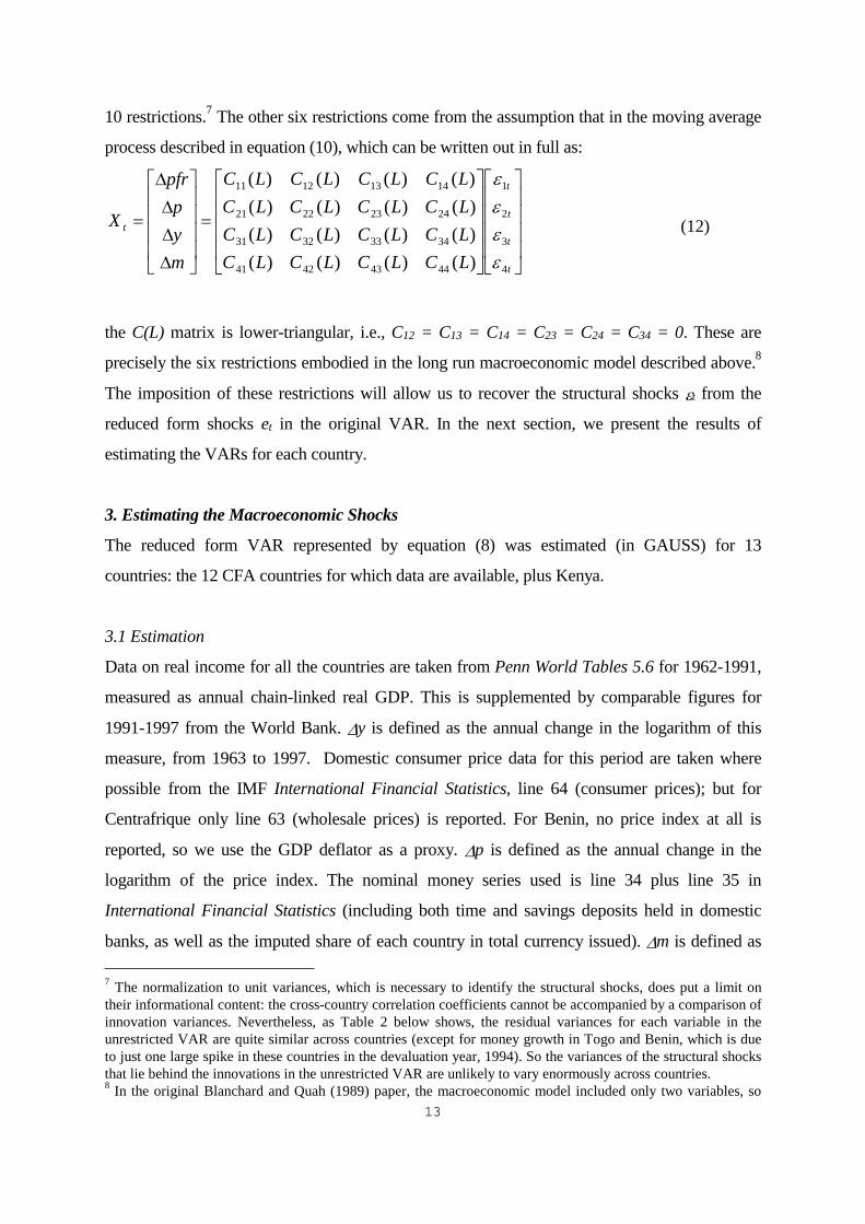
10 restrictions.7 The other six restrictions come from the assumption that in the moving average

process described in equation (10), which can be written out in full as:

)()()()()()()()()()()()()()()()(

4

3

2

1

44434241

34333231

24232221

14131211

⎥⎥⎥⎥

⎦

⎤

⎢⎢⎢⎢

⎣

⎡

⎥⎥⎥⎥

⎦

⎤

⎢⎢⎢⎢

⎣

⎡

=

⎥⎥⎥⎥

⎦

⎤

⎢⎢⎢⎢

⎣

⎡

∆

∆

∆

∆

=

t

t

t

t

t

LCLCLCLCLCLCLCLCLCLCLCLC

LCLCLCLC

myp

pfr

X

ε

ε

ε

ε

(12)

the C(L) matrix is lower-triangular, i.e., C12 = C13 = C14 = C23 = C24 = C34 = 0. These are

precisely the six restrictions embodied in the long run macroeconomic model described above.8

The imposition of these restrictions will allow us to recover the structural shocks εt from the

reduced form shocks et in the original VAR. In the next section, we present the results of

estimating the VARs for each country.

3. Estimating the Macroeconomic Shocks

The reduced form VAR represented by equation (8) was estimated (in GAUSS) for 13

countries: the 12 CFA countries for which data are available, plus Kenya.

3.1 Estimation

Data on real income for all the countries are taken from Penn World Tables 5.6 for 1962-1991,

measured as annual chain-linked real GDP. This is supplemented by comparable figures for

1991-1997 from the World Bank. ∆y is defined as the annual change in the logarithm of this

measure, from 1963 to 1997. Domestic consumer price data for this period are taken where

possible from the IMF International Financial Statistics, line 64 (consumer prices); but for

Centrafrique only line 63 (wholesale prices) is reported. For Benin, no price index at all is

reported, so we use the GDP deflator as a proxy. ∆p is defined as the annual change in the

logarithm of the price index. The nominal money series used is line 34 plus line 35 in

International Financial Statistics (including both time and savings deposits held in domestic

banks, as well as the imputed share of each country in total currency issued). ∆m is defined as

7 The normalization to unit variances, which is necessary to identify the structural shocks, does put a limit on their informational content: the cross-country correlation coefficients cannot be accompanied by a comparison of innovation variances. Nevertheless, as Table 2 below shows, the residual variances for each variable in the unrestricted VAR are quite similar across countries (except for money growth in Togo and Benin, which is due to just one large spike in these countries in the devaluation year, 1994). So the variances of the structural shocks that lie behind the innovations in the unrestricted VAR are unlikely to vary enormously across countries. 8 In the original Blanchard and Quah (1989) paper, the macroeconomic model included only two variables, so

14

the annual change in the logarithm of this measure. The foreign price series is measured as the

French consumer price index multiplied by the CFA Franc – French Franc exchange rate (or in

the case of Kenya by the Shilling – French Franc exchange rate); ∆pfr is defined as the change

in the logarithm of this series. In this way the evolution of domestic income, money and prices

is conditioned on the same foreign price shock in all countries. Adjusting the definition of ∆pfr

to include a trade-weighted basket of currencies did not make a substantial difference to the

results. The full data set is available on request. Appendix 1 discusses stationarity tests for the

variables are interest; in all cases a null hypothesis of non-stationarity can be rejected.

If we were estimating a VAR for a single country then an OLS estimate would be

efficient, since lags of all the endogenous variables appear in all of the equations, and we would

not need to bother to estimate a residual covariance matrix. But in a model with several

countries there is a potential efficiency gain from using a SUR estimator to capture cross-

country residual correlations. It is not possible to estimate a complete covariance matrix for the

residuals from every equation using annual data for 1963-97: altogether in our model there are

39 time series for domestic income, money and price growth. Nevertheless, we can estimate

cross-country covariance matrices for each variable in the model by stacking the ∆p equations

for each country and estimating them by SUR, and then doing the same for ∆y and ∆m. This will

be asymptotically more efficient than OLS, but does not allow for correlation between, say, ∆p

in one country and ∆y in another.

Table 2 presents summary diagnostic statistics for equations estimated in this way. In

each of the three SUR estimates (for ∆p, ∆y and ∆m) the equations have been estimated with a

lag order of two; this choice is made on the basis of the Akaike Information Criterion. The

regression R2s vary considerably, but are is typically between one third and one half, and are

greater for ∆p than for ∆y and ∆m. These proportions are perhaps a little smaller than the figures

one might expect for a typical OECD country or NIC: the Franc Zone is made up of very small

open economies which suffer from large shocks. There is no significant autocorrelation in any

of the reduced form residuals. Table 2 also reports summary statistics for the foreign price

inflation equation, which is modeled as an autoregressive process. For each individual country

VAR, the set of regressors is jointly significant at the 1% level, though individual coefficients

are sometimes insignificant; the same is true of each stack of variables across countries.9

the C(L) matrix was 2 x 2 and only one theoretical restriction was required to make it lower-triangular. 9 The corresponding F-statistics are not reported in Table 2, but are available on request.

15

Table 2: Regression Diagnostic Statistics

y Equation R2 S.E. D.W. ben 0.01 0.05 1.95 bfa 0.36 0.03 2.26 civ 0.30 0.05 1.84 sen 0.52 0.03 2.13 tgo 0.08 0.06 1.93 mli 0.36 0.03 1.84 ner 0.20 0.08 2.04 cmr 0.46 0.04 1.51 cgo 0.31 0.06 1.54 gab 0.30 0.08 2.25 car 0.03 0.04 1.37 tcd 0.35 0.10 2.13 ken 0.30 0.06 2.08

p Equation R2 S.E. D.W. ben 0.32 0.06 2.08 bfa 0.42 0.06 2.28 civ 0.35 0.05 1.63 sen 0.61 0.05 1.93 tgo 0.55 0.05 1.90 mli 0.60 0.06 2.08 ner 0.48 0.06 1.66 cmr 0.45 0.05 1.92 cgo 0.41 0.04 1.81 gab 0.75 0.04 1.77 car 0.64 0.04 2.02 tcd 0.60 0.04 1.77 ken 0.50 0.07 1.79

m Equation R2 S.E. D.W. ben 0.42 0.24 2.34 bfa 0.22 0.09 1.53 civ 0.22 0.09 1.80 sen 0.28 0.13 2.24 tgo 0.33 0.29 2.30 mli 0.12 0.11 1.63 ner 0.29 0.11 2.11 cmr 0.46 0.09 2.39 cgo 0.20 0.11 2.37 gab 0.58 0.10 2.25 gar 0.08 0.12 1.70 tcd 0.16 0.16 2.24 ken 0.10 0.08 1.98

pfr Equation R2 S.E. D.W. cfa 0.82 0.02 2.02 ken 0.04 0.11 2.01

16

These estimates are used to construct the reduced form innovation matrix et for each

country. Imposing the restrictions outlined in the previous section allows us to construct the

corresponding normalized structural innovation matrix εt. We do not report detailed estimates of

each equation in each country, but these are available on request. In each country the asymptotic

impulse responses implicit in the estimated model (that is, the estimated elements of the lower-

triangular matrix C(L) in equation (12)) are theory-consistent in the sense that they either have a

value consistent with the signs of the parameters of the theoretical model represented by

equations (2) and (5-7), or are insignificantly different from zero.

In the rest of this section we present three features of interest in the regression results:

the cross-country correlation coefficients for the price shocks in the structural model, the

corresponding coefficients for the income shocks, and the corresponding impulse responses in

the different countries.10

3.2 Price shock correlation coefficients

The full set of cross-country correlation matrices for each element of εt is reported in full in

Appendix 2, along with corresponding t-ratios and cross-country correlation coefficients for et.

Tables 3-8 summarize the information in Appendix 2.

For the ith member of the UEMOA, or of the BEAC region, one can compute

coefficients of the correlation of each element of εt with the corresponding element for another

country. For each element, averaging over the correlation coefficients with respect to that

member’s partners (six in the UEMOA, four in the BEAC region) gives a measure of the degree

of similarity of between shocks to that element in the ith country and shocks in its partners. Such

averages are shown in the right-hand columns of Tables 3-4. Averages are shown for the two

elements of εt relevant to the questions raised in Section 1: the innovations in ∆p and ∆y. The

number of significant correlation coefficients (“+” for positive correlations and “-” for negative

ones) is shown in parenthesis. If there are both significantly positive and significantly negative

correlation coefficients, the term “mixed” appears in parenthesis. The reduced form et

correlation averages are also noted in the left-hand columns for comparison.

Tables 5-6 show similar average correlation figures, but for the average correlation

between a shock to one country and shocks to countries in the other monetary union. If these are

larger (positive) numbers than in Tables 3-4, then the country is in some sense more similar to

10 Since the shocks in the εt matrix are normalized with a unit variance we do not report the standard errors of structural shocks.

17

the members of the other union than it is to its existing partners. If the numbers are the same,

then the country is as similar to the members of the other union as it is to its existing partners.

Tables 7-8 show correlation coefficients for each CFA member vis a vis Kenya, to give a sense

of the extent to which the CFA countries exhibit more similarity amongst themselves than any

does to a representative non-CFA member.

For all CFA members, the averages of the price innovation correlation coefficients are

large – mostly around 0.7 - and significantly different from zero. (And they are generally bigger

than the correlation coefficients from the reduced-form price equation, so a structureless VAR

tends to underestimate the degree of similarity in price shocks.) In other words, if we put a lot of

weight on the importance of initial price shocks in assessing the costs and benefits of a

monetary union, and less weight on initial income shocks or on the eventual impact of a price

shock on the whole economy, then the CFA comes out quite well. Price shocks tend to be quite

highly correlated across member states, and on average a monetary policy response based on the

average price shock to member states in one particular period will be appropriate for all

countries individually. This conclusion would still be true if policy were weighted towards the

largest members of the CFA (Cote d’Ivoire in the UEMOA and Cameroon in the BEAC region).

As shown in Table A3 in Appendix 2, these two countries’ price innovation correlation

coefficients with respect to their partner states are all around 0.9, with two exceptions discussed

below.

Moreover, there is generally no significant difference between a country’s average price

innovation correlation with its existing partners (Tables 3-4) and the average with the members

of the other monetary union (Tables 5-6). There is no particular economic need for the border

between the UEMOA and the BEAC region: a single monetary union would do as well.

There are however two countries for which the average correlation coefficients are a

little lower than the rest, though still significantly positive: Niger in the UEMOA and Chad in

the BEAC region. For Niger the average correlation coefficient is about 0.4 and for Chad about

0.5. These are both Sahelian economies on the northern edge of the CFA area with very little in

the way of industry or mineral exports. In these countries a monetary policy response tailored to

the cross-country average shock to the monetary union, or to the shock in its dominant

member(s), would typically only roughly correspond to the ideal policy for the country.

For no CFA member is it possible to reject the null that its structural price innovations

are orthogonal to those of Kenya (Tables 7-8). These innovations have been estimated in a

18

model which conditions on money supply growth and foreign prices, so the result cannot be

explained by the fact that a common monetary policy was pursued in CFA members that was

different from the policy in Kenya. However, it is not possible to determine whether the

differences between the CFA and Kenya are due to differences in the underlying economic

structure of the Kenyan economy that would not have arisen had it been part of a CFA-style

monetary union. The Kenyan economy has at times exhibited characteristics (such as extreme

financial repression) that have not arisen in the CFA. All that can be said is that given the

existing structure of the Kenyan economy, its price shocks, controlling for shocks to the money

supply, are unlike those of the CFA.

3.3 Output innovation correlation coefficients

The correlation coefficients for structural innovations to income growth are rather different. In

both the UEMOA and the BEAC region there are some significantly negative and some

significantly positive coefficients for within-union shocks (Tables 3-4). The full correlation

matrix is shown in Table 9, which shows the source of this asymmetry. There are two groups of

CFA countries within which all the coefficients are significantly positive, and between which all

the coefficients are significantly negative. The two groups are:

(i) Benin, Burkina Faso, Senegal, Togo, Niger, Cameroon, Gabon, Centrafrique, Chad

(ii) Cote d’Ivoire, Mali, Congo Republic

Within these groups, the correlation coefficients are mostly in the range 0.5 to 0.9; between the

groups, the correlation coefficients are mostly in the range –0.5 to –0.9. The second, smaller

group contains the two most indebted UEMOA members: Cote d’Ivoire, and its economically

small neighbor Mali, which lies on the northern border of Cote d’Ivoire and provides the Ivorian

economy with many migrant workers. It is not entirely surprising that Cote d’Ivoire and its

northern satellite should exhibit some similarity in terms of shocks to aggregate supply and

aggregate demand, and differ from the other members of their monetary union.

It is a little more surprising that the third member of the group is Congo Republic, a

petroleum exporter and BEAC member at the southern edge of the Franc Zone. It is certainly

difficult to see why Congo’s aggregate supply shocks should exhibit more similarity with Cote

d’Ivoire than with Gabon and Cameroon. The features that Congo has in common with the other

19

Table 3

UEMOA Countries: Average Innovation Correlations with the Rest of their Union

(Number and sign of significant correlations in parenthesis)

∆p reduced form ∆p structural model

ben 0.30 (3+) 0.61 (6+) bfa 0.34 (5+) 0.66 (6+) civ 0.31 (3+) 0.69 (6+) sen 0.19 (2+) 0.68 (6+) tgo 0.34 (4+) 0.70 (6+) mli 0.08 (0+) 0.67 (6+) ner 0.30 (3+) 0.39 (6+)

∆y reduced form ∆y structural model

ben -0.12 (2-) 0.07 (mixed) bfa -0.03 (1-) 0.17 (mixed) civ 0.01 (1-) -0.38 (mixed) sen 0.07 (0+) 0.14 (mixed) tgo 0.06 (1+) 0.14 (mixed) mli 0.17 (1+) -0.40 (mixed) ner 0.09 (0+) 0.17 (mixed)

Table 4

BEAC Countries: Average Innovation Correlations with the Rest of their Union



cmr 0.26 (1+) 0.69 (4+) cgo 0.25 (2+) 0.69 (4+) gab 0.18 (1+) 0.69 (4+) car 0.29 (3+) 0.69 (4+) tcd 0.17 (1+) 0.51 (4+)


cmr -0.01 (0+) 0.27 (mixed) cgo -0.04 (1-) -0.64 (4-) gab 0.07 (1+) 0.27 (mixed) car 0.12 (1+) 0.25 (mixed) tcd -0.14 (0+) 0.25 (mixed)

20

Table 5

UEMOA Countries: Average Innovation Correlations with BEAC Countries



ben 0.37 (3+) 0.74 (5+) bfa 0.32 (2+) 0.79 (5+) civ 0.37 (4+) 0.85 (5+) sen 0.24 (2+) 0.87 (5+) tgo 0.27 (2+) 0.84 (5+) mli 0.20 (0+) 0.87 (5+) ner 0.19 (1+) 0.35 (5+)


ben -0.11 (mixed) 0.22 (mixed) bfa 0.21 (1+) 0.38 (mixed) civ 0.09 (1+) -0.34 (mixed) sen -0.07 (0+) 0.29 (mixed) tgo 0.28 (1+) 0.44 (mixed) mli 0.16 (2+) -0.41 (mixed) ner 0.05 (mixed) 0.38 (mixed)

Table 6

BEAC Countries: Average Innovation Correlations with UEMOA Countries



cmr 0.23 (1+) 0.78 (6+) cgo 0.37 (3+) 0.81 (7+) gab 0.21 (2+) 0.82 (7+) car 0.37 (4+) 0.82 (7+) tcd 0.23 (2+) 0.56 (6+)


cmr 0.04 (1+) 0.26 (mixed) cgo 0.09 (1+) -0.29 (mixed) gab 0.03 (1-) 0.28 (mixed) car 0.18 (mixed) 0.22 (mixed) tcd 0.09 (mixed) 0.22 (mixed)

21

Table 7

UEMOA Countries: Innovation Correlations with Kenya

(t-ratios in parenthesis)


ben -0.06 (-0.32) -0.15 (-0.83) bfa 0.07 ( 0.36) 0.07 ( 0.39) civ -0.07 (-0.35) 0.02 ( 0.10) sen -0.00 (-0.00) 0.04 ( 0.19) tgo -0.17 (-0.92) -0.04 (-0.23) mli -0.34 (-1.94) -0.08 (-0.41) ner -0.23 (-1.25) 0.05 ( 0.26)


ben -0.22 (-1.21) -0.32 (-1.78) bfa 0.32 ( 1.81) -0.02 (-0.08) civ -0.28 (-1.54) 0.17 ( 0.90) sen -0.18 (-0.95) -0.07 (-0.37) tgo -0.27 (-1.47) -0.18 (-0.99) mli 0.01 ( 0.07) 0.09 ( 0.49) ner -0.46 (-2.78) -0.25 (-1.39)

Table 8

BEAC Countries: Innovation Correlations with Kenya

(t-ratios in parenthesis)


cmr -0.41 (-2.37) -0.09 (-0.46) cgo -0.24 (-1.32) -0.01 (-0.05) gab -0.20 (-1.08) -0.01 (-0.07) car -0.22 (-1.19) -0.01 (-0.05) tcd -0.23 (-1.23) -0.31 (-1.72)


cmr 0.03 ( 0.16) -0.04 (-0.22) cgo -0.56 (-3.54) 0.10 ( 0.53) gab 0.13 ( 0.68) -0.05 (-0.25) car -0.19 (-1.00) 0.06 ( 0.33) tcd 0.33 ( 1.87) 0.25 ( 1.37)

22

Table 9: Output Shock Correlations

ben bfa sen tgo ner cmr gab car tcd civ mli cgo

ben 1 0.47 0.13 0.56 0.38 0.52 0.48 0.31 0.28 -0.58 -0.48 -0.5 bfa 0.47 1 0.68 0.78 0.76 0.69 0.84 0.54 0.67 -0.73 -0.77 -0.83 sen 0.13 0.68 1 0.58 0.79 0.56 0.63 0.4 0.55 -0.56 -0.64 -0.68 tgo 0.56 0.78 0.58 1 0.85 0.81 0.9 0.67 0.77 -0.87 -0.93 -0.93 ner 0.38 0.76 0.79 0.85 1 0.76 0.82 0.58 0.65 -0.8 -0.83 -0.9 cmr 0.52 0.69 0.56 0.81 0.76 1 0.87 0.62 0.69 -0.74 -0.76 -0.83 gab 0.48 0.84 0.63 0.9 0.82 0.87 1 0.69 0.75 -0.82 -0.88 -0.93 car 0.31 0.54 0.4 0.67 0.58 0.62 0.69 1 0.61 -0.42 -0.57 -0.66 tcd 0.28 0.67 0.55 0.77 0.65 0.69 0.75 0.61 1 -0.61 -0.79 -0.8

civ -0.58 -0.73 -0.56 -0.87 -0.8 -0.74 -0.82 -0.42 -0.61 1 0.86 0.87 mli -0.48 -0.77 -0.64 -0.93 -0.83 -0.76 -0.88 -0.57 -0.79 0.86 1 0.94 cgo -0.5 -0.83 -0.68 -0.93 -0.9 -0.83 -0.93 -0.66 -0.8 0.87 0.94 1

countries in group (ii) are a high debt level and a low reliance on trade taxes for government

expenditure (see Table 1). In the light of the discussion at the end of Section 2.1, it may be that

these features reflect a commonality in the nature of shocks to aggregate demand.

In the absence of interest rate data it has not been possible to identify aggregate demand

shocks separately from aggregate supply shocks: the estimated innovations in ∆y are the sum of

both together. One interpretation of the results here is that aggregate demand shocks dominate

aggregate supply shocks (otherwise we should see commonality in the shocks to ∆y in the

petroleum exporters), and that the nature of aggregate demand shocks is linked to indebtedness.

The VAR modeling framework is not well suited to picking out the structure of such links, but

suggests a potentially fruitful line of complementary country-specific research into the links

between fiscal policy and aggregate demand shocks.

Nevertheless, the results here suggest that if we put a lot of weight on the importance of

initial output shocks in assessing the costs and benefits of a monetary union, and less weight on

initial price shocks, then the CFA should be reorganized. It would be more appropriate for Cote

d’Ivoire and Mali to form one monetary union (possibly joined by Congo Republic), and for the

other existing CFA members to join together to form another.

3.4 Long Run Impulse Responses

The information in Tables 3-9 relates to the characteristics of structural shocks to the economies

23

of the CFA. In a world where monetary authorities respond in a timely way to price and output

shocks to their economies the long run effect of shocks is not of immediate concern: the shock

will have been sterilized before its long run effect is realized. In a world where monetary

authorities are slower to respond this is no longer true, and we must examine the impact of price

and output shocks on the economic system over a longer time horizon.

Using the structural VAR we have estimated, it is possible to draw an impulse response

function for the impact of each shock on each variable in each of the 13 countries. Rather than

reproducing all of these charts, we will focus on the asymptotic effect of each shock on each

variable. Table 10 summarizes the information in the impulse response functions by listing the

long run responses to each shock, i.e., the total area underneath each impulse response curve.

The points we have to make below would not be substantially altered if we instead reported

figures for the areas below the impulse response curves up to a finite time horizon.

So Table 10 shows the long run effects on each economy of both a unit shock to

inflation and a unit shock to output growth. Given the structure of our model, inflation shocks

have a long run impact on both prices and output, whereas output growth shocks have an

effect only on prices, so there are three columns of figures in Table 10.11 The figures show the

eventual impact of a one-period shock to inflation and output growth on the level of prices

and output; for example, a figure of 0.1 implies that the level will increase by 10%.

The most striking aspect of Table 10 is the large cross-country variance in the

estimated impulse responses. It is true that the long run effects of inflation shocks on

inflation, and of output growth shocks on output growth, are all positive, and that the long run

effect of a shock is smaller than the initial impact: all the figures in the first and third columns

of Table 10 are in the interval [0,1]. However, the size of the inflation effect varies between

0.08 (Cameroon) and 0.73 (Benin), and the size of the output growth effect varies between

0.13 (Senegal, Congo Republic) and 0.48 (Chad). In some countries the initial shock is

quickly dissipated, so that the long run effect on the level of the variable is very small; in

others, the rate of dissipation is much slower, so the long run effect is quite large. If monetary

authorities responded to shocks only after a considerable delay, response appropriate in each

country would vary widely across the Franc Zone. In other words, the costs of CFA

membership in terms of lost monetary autonomy will be much larger than in a world where

the monetary response to a shock is immediate.

This conclusion is reinforced by the figures in the second column of Table 10, which

is the franc zone an optimal currency area?

Documents