Discussion Papers No. 166 • Statistics Norway, February 1996

John K. Dagsvik

Consumer Demand withUnobservable Product AttributesPa rt I: Theory

Abstract:Th is paper develops a new framework for empirical modelling of consumer demand with particular referenceto products that are differentiated with respect to quality and location attributes. The point of departure is aflexible representation of the distribution of product attributes and consumer tastes. From this representationand additional behavioral assumptions we derive a structural model for the distribution of the chosenproduct attributes and the associated quantities. Furthermore, an explicit relationship between thedistribution of prices and unit values is obtained.

Keywords: Price distribution, differentiated products, quality attributes, hedonic price indexes.

JEL classification: C25, C43, D11

Acknowledgement Thanks to R. Aaberge, J. Aasness and T.J. Klette for valuable comments and AnneSkoglund for correcting typos.

Address: John K. Dagsvik, Statistics Norway, Research Department,P.O.Box 8131 Dep., N-0033 Oslo, Norway. E-mail: jda@ssb.no

.

1. Introduction

The textbook theory of consumer demand assumes that the products consumed are

homogeneous. This is obviously a rather stylized setting since a typical feature is that

products are differentiated with respect to quality attributes. Also prices may vary with respect

to these attributes as well as with respect to geographical location of the stores. This paper

develops a new framework for analyzing consumer demand for differentiated products in the

presence of quality- and location attributes when some of these attributes are unobservable

to the analyst.

Following Lancaster (1979), p. 16; "the problem of analyzing economic systems in

which the goods (or many of them) can be infinitely varied in design and specification has

always been that of finding a workable framework of analysis." The traditional way of dealing

with quality aspects is either simply to increase the number of goods or to apply Hicks

aggregation. Unfortunately, in practice it turns out to be difficult to treat each variant as a

separate observable commodity category. This is related to the fact that it is problematic to

quantify quality precisely. In other words, quality is typically a latent variable which only to

a limited extent can be accounted for by classifying variants of the product under

consideration into a large number of categories. Although many variants can in principle be

classified in observable categories, there will, in practice, be a limit to how many variants one

can treat as separate goods in a demand system. To aggregate goods into composite ones is

also problematic. If consumers have heterogeneous preferences the corresponding price

indexes will be individual specific and can therefore not readily be implemented in empirical

demand analyses!

When unobserved quality attributes are present the econometrician faces a simultaneity

problem. The reason for this is that the random terms in the demand system depend on latent

quality attributes, which in turn are correlated with prices. It is known (see for example

Trajtenberg (1989)) that ignoring this simultaneity problem can lead to upward sloping

demand curves. Moreover, the aggregate demand function in the presence of differentiated

products may depend on the whole distribution of prices—not only on the mean price across

all variants of each product.

It seems that some authors, such as Chamberlin (1933), p. 79, have thought it impossible to carry through afull formal analysis of variable product design: ...."product variations are in this essence quantitative; they cannot,therefore, be measured along an axis and displayed in a single diagram".

3

Early studies that discuss this problem are the contributions by Houthakker and Prais

(1952 and 1955). While most early work was concerned with practical problems of

econometrics within a simple theoretical framework, contributions such as Fisher and Shell

(1971), Muellbauer (1974) and Lancaster (1979) have dealt with the theoretical foundations.

Rosen (1974), Bartik (1987), Epple (1987), Brown and Rosen (1982) and Berry et al. (1995),

analyse the econometric problems related to estimating demand and supply of differentiated

products. Deaton (1987, 1988) analyses demand in the presence of price variation due to

heterogeneity with respect to latent quality aspects and spatial location of stores, with

particular reference to developing countries. The reason why spatial variation in prices may

occur is because transportation is expensive and it may also be the case that different stores

offer different types of services.

The approach taken here differs from the contributions above. First, the choice setting

is viewed as a discrete/continuous one where the discrete dimension corresponds to the

product variants. Thus, in contrast to the framework which is commonly used (see for

example Rosen (1974)) we perceive the consumer as making his choice from a set of discrete

"packages" of attribute combinations. Second, the random variables associated with

unobserved product attributes and taste-shifters are, similarly to Dagsvik (1994), treated as

integral parts of the choice model. The basic idea of the approach is as follows: Consumers

face a variety of product variants and locations, each of which is characterized by its price

and a variable that may be interpreted as a "quality" index, cf. Lancaster (1977). This quality

index may depend on observable product characteristics (attributes). We thus represent a

consumer's set of feasible variants/locations by a collection of pairs of prices and quality

indexes. Specifically, this set of prices and quality indexes may be summarized in a

distribution function which represents the fraction of feasible variants/locations with prices

and quality indexes less than or equal to a given level of price and quality. As mentioned

above, the consumers are assumed to have preferences over variants/locations which governs

their choice of products and the corresponding quantities. To this end a particular

discrete/continuous random utility choice model is developed, in which the probability

distribution of the prices and quality indexes of the chosen variants/locations is expressed as

a function of parameters of the consumers utility functions and the distribution of prices and

quality indexes associated with the feasible location/variants. In other words, the fraction of

(observational identical) consumers who choose variants/locations with a given price and

4

quality is in this model expressed as a function of the distribution of preferences and offered

prices and quality attributes. In the presence of latent quality/location attributes and

unobserved heterogeneity in preferences, the distribution of unit values, i.e., expenditure to

quantity for each commodity, may differ from the distribution of prices. That is, the number

of (latent) variants in the market within a commodity group (observable) with prices below

a given level may differ from the corresponding number of variants purchased by the

consumers. This is due to a selection effect that arises from consumers having preferences

over the variants. By means of the model developed below it is possible to derive a

convenient expression for the distribution of unit values as a function of the distribution of

prices and parameters related to preferences. Furthermore, one can construct price indexes

(which we denote virtual prices) for each (observational) commodity group which account for

the possibility that consumers have preferences over variants/locations that are unobservable

to the analyst. As a result, it follows that the chosen quantities, within the commodity groups,

can be expressed as in a conventional demand system with prices replaced by virtual prices.

Although the virtual prices are unobservable random variables it is possible to identify and

estimate their probability distribution function. Accordingly, one can identify and estimate

parameters of the demand system. In Put II of this paper we discuss estimation issues related

to the framework developed in Part I.

Among the contributions mentioned above, the paper by Berry et al. (1995) is the one

which is the closer to the present paper. However, in contrast to this paper, Berry et al. only

consider the discrete choice case and they also assume that the classification of product

variants relevant to the consumer is observable to the analyst.

The paper is organized as follows: In Sections 2 and 3 we present the theoretical

model and we derive the distribution function for the demand and for the unit values. In

Section 4 we discuss identification in a modified AIDS demand system, cf. Deaton and

Muellbauer (1980). The final section is devoted to the case where consumers only buy one

unit of a product at a time. In this section we also introduce observable (nonpecuniary)

product attributes.

5

2. A model for individual purchase that accounts for horizontal and vertical productdifferentiation: The basic assumptions

A major problem the analyst faces when dealing with the demand for differentiated

products is that taste-shifters and quality attributes that affect preferences are unobservable.

Below we shall introduce a particular framework that enables us to analyze consumer demand

under aggregation of quality/location attributes.

Consider a consumer (household) which faces a set of products characterized by

quality attributes and price. There are m categories of goods indexed by j, j=1,2,...,m. Within

each category, let z=1,2,..., index an infinite set of stores (location of the stores) and product

variants that are offered for sale in the market. For example, the categories may be beer and

cereals in which case the corresponding variants are the brands of beer and cereals. Let Q(z)

be the quantity of observable type j and unobservable location and variant z and let Ti(z)>O,

be an unobservable quality/location attribute associated with good (j,z), The attributes

{Ti(z)} are objectively measured in the sense that all consumers' perceptions about

aggregation and ranking of characteristics embodied in each good are identical. Consistent

with Lancaster (1979), p. 27, the T-attributes correspond to the notion of vertical product

differentiation. If some characteristics associated with the variants are observable, {Ti(z)} can

be specified as a function of z-specific observable attributes. In this case Tj will be a

(hedonic) quality index. Let P(z) be the price of variant/location z of type j. As regards the

spatial dimension, a natural "unit" is the store because prices of a given variant do not vary

within stores. In general, Pi(z) and Ti(z) may be correlated, cf. Stiglitz (1987). How the

distribution of prices and T-attributes is determined in the market will briefly be discussed

below. The consumer is assumed to be perfectly informed about the distributions of product

locations, variants and prices.

Let

(Q*,T*) p i (1),T 1 (1),Q 1 (2),T 1 (2),...,Q2(1),T2(1),Q2(2), T2(2), ...,Qm(

represent the bundle of quantities and quality attributes of different types and variants.

Without loss of generality we may rearrange the components of (Q* ,T*) as

6

(Q, x p i (z), T (z),Q2(z),T2(z), ..,Qm(z), T.(z))

which is notationally more convenient than (Q*,T*). The setup above is analogous to the

characteristics approach of Lancaster (1966), where {T(z)} represents the characteristics

dimension. The enumeration in different commodity categories are of course totally

indpendent.

Let U(Q,T) be the associated utility of a (particular) consumer. We make the

following assumption:

Assumption Al

The utility function has the structure U(Q,T) = u(S1,S2,...,S„), where

= E Q/z)7;(z)Vz), (2.1)

u() is a mapping, u:R.--->k, that is increasing and quasi-concave, and ( k(z), z=1,2,...) are

random positive- taste-shifters that account for unobservable variables that reflect

heterogeneity in consumer taste.

Note that the interpretation of the taste-shifters, { k(z)}, is also consistent with

psychological choice theories in which the decision maker is seen as having difficulties with

assessing the precise value (to him) of the consumption bundle. Thus, this notion accounts

for unobserved variables that affect preferences and are known to the household as well as

factors that affect preferences and are random to the household.

The utility structure (2.1) implies that within subgroup j the different qualities are

perfect substitutes, cf. Haneman (1984), p. 548. A consequence of (2.1) is thus that the

consumer will only buy one quality variant at a time, i.e., for a given set of taste-shifters,

7

{ ti(z), z=1,2,..., j=1,...}, only one variant will be chosen.2 Thus this setup is a version of the

"Ideal Variety Approach" proposed by Lancaster (1979). Krugman (1989) argues that the

Ideal Variety Approach is more realistic than the "Love of Variety Approach" proposed by

Spence (1976), and Dixit and Stiglitz (1977). The structure in (2.1) is also analogous to the

models investigated by Fisher and Shell (1971), and Gorman (1976). According to Lancaster,

op cit. the taste-shifters, { i(z)}, correspond to the notion of horizontal product differentiation.

In the special case where the only latent choice variable is associated with location,

i.e., z indexes the stores, then the assumption that the consumer only chooses one z at a time

seems natural since it may be fair to view the consumer as choosing a single store each time

he goes shopping.

Yet another interpretation is possible: We may think of z as an indexation of (latent)

"categories", or "baskets", of which basket z, say, consists of "similar" commodities.

Examples of baskets are; sports gear and breakfast menus.

Now let us return to the general analysis, where we shall proceed to derive the

structure of the demand functions. The budget constraint is given by

E E Q(z)P(z) y.z (2.2)

In order to link the present setup to conventional demand theory we shall now introduce some

additional notation that will facilitate the formal analysis. Let

Rj(z) = Pi(z)/(ti(z)Tj(z)) . (2.3)

If (2.3) is inserted into (2.2) we can express the budget constraint as

2The formulation postulated in (2.1) is less restrictive than it appears: We may namely interpret (2.1) asrepresenting the consumer's preferences at a specific moment of purchase — where we allow the set of taste-shifters change each time the consumer goes shopping — or fixed within a short period of time. Of course, thisinterpretation entails questions about aggregation over time and about the consumers planning horizon. Theproblem of assessing a realistic planning horizon is also important for the interpretation of data fromconventional expenditure surveys since these surveys typically contain data on household expenditure based onshort periods of observation (one to three weeks), while a more reasonable notion of "period" in a (static) modelis perhaps one year. In Appendix B we outline a possible simple approach for modifying the model so as toallow for savings/borrowing within a year.

E E Si(z)Ri(z) y (2.4)

z

where

S( z) Qi(z) Ti(z);(z).

Note that maximizing u(S i ,S2,...,Sm) subject to (2.2) is equivalent to maximizing

u(E s l (z),E sm(z))1,

subject to (2.4). Moreover, this optimizing problem is formally equivalent to a conventional

consumer demand problem where Sj(z), z=1,2,..., are perfect substitutes with corresponding

"prices", {Rj(z)}. Thus, we realize that this implies that the consumer will choose only one

(unobservable) quality variant within each observable category. Let 2 be the index of the

chosen store and variant within category j. Clearly, Zi is determined by

R.(2.) = min Ri(z),J J (2.5)

which mean that 2j is the variant with the lowest "price". For notational simplicity, let ki

R(î), 4 = Qi(2j), Šj = S() and Pi = Pj(2j). Let Ri(r,y) be the expenditure of type j that

follows from maximizing

subject to

UtS S S2"*"

E r.s. 5_ y,J

(2.6a)

(2.6b)

where r=(r 1 ,r2,..., . Evidently, we have that

š.k. 7(..(fi, y)= =

P. P.J

.1 J(2.7)

where

= (Apkr..- , Am).

Thus, from (2.7) we realize that formally, we can account for the heterogeneity in quality and

prices by replacing prices in an ordinary demand (expenditure) system by the corresponding

components of k. We shall call {Ri } virtual prices. The virtual price vector, is endogenous

since by (2.5) it is the result from the consumer's choice of location and quality (2). The

virtual prices are taste-and-quality-adjusted-prices in the sense that if these virtual prices were

known, consumer behavior could be represented by an ordinary demand system that does not

depend on quality attributes nor taste-shifters. Note that the virtual prices are unobservable.

Note also that {f} represent unit values, i.e., the respective ratios of expenditure to quantity

for each commodity, and they therefore depend on the consumer's choice.

To obtain analytic expressions we need to make further assumptions about the

distribution of the unobservables. Recall that according to the setup above each

variant/location z of type j is characterized by the attribute vector (Pi(z),Ti(z),4i(z)) where

(Pi(z),Ti(z)) are objectively perceived attributes in the sense that they have the same value

relative to any consumer, while 4i(z), (for fixed (j,z)) may vary across consumers — or over

time for a given consumer. Let

pi = Oi(z),Ti(z),;(z)), = 1,2,. ..}

denote the (consumer-specific) collection of prices, quality attributes and taste-shifters

associated with the feasible variants/stores. To make the setup above operational we need to

introduce assumptions about the distribution of the elements in p i . The next assumption is a

convenient representation of the distribution of taste-shifters and feasible attributes (prices and

quality attributes).

Assumption A2

The vectors in Pi, j=1,2,...,m, are points of independent inhomogeneous Poisson

processes on R34. with intensity measure associated with Pi equal to

10

Gi(dp,dt) pi(e)dE. (2.8)

Moreover, the Poisson points associated with different consumers are realizations from

independent copies of the Poisson process.

Recall that the Poisson process framework means that the (vector) points in Pj are

independently distributed and the probability that there is a point in Pj for which

Pi(z)e (p,p+dp), Ti(z)E (t,t+dt) and tj(z)e (E,e+de) is equal to Gi(dp,d0pi(E)cle.

The reason why the Poisson points differ across consumers is because the taste-shifters

ki(z)} are individual specific: Different consumers evaluate the variants differently and the

tastes of a given consumer may also fluctuate randomly over time. The fact that the value of

a store to a given consumer may depend on the distance between him and the store is also

captured in this formulation. Note that this formulation allows prices to vary across products

with given quality. As mentioned in the introduction, a rationale for this is that prices may

vary across stores because different stores/producers have different cost functions due to

transportation and the quality of the services offered by the stores.

In Dagsvik (1994) it is demonstrated that Gi(p,t) can be interpreted as the distribution

of feasible prices and quality attributes. This means that Gi(p,t) is the fraction of all variants

of type j in the market that have prices and quality attributes less than or equal to (p,t). The

multiplicative structure of (2.8) means that the taste-shifters are independent of the prices,

location and quality attributes. A justification for assuming the prices and quality attributes

be independent of the taste-shifters stems from the view that the market forces operate on an

aggregate level in the sense that the respective distributions of supply and demand are

dependent. This means that the intensity measure (2.8) has a functional form that depends

both on the systematic parts of the consumers' utility functions and the producers' profit

functions. However, the distribution of supply and demand may not necessarily coincide

because the firms may have limited information about the distribution of demands when (and

if) they set prices. To perform policy analyses (in a rigorous sense) requires a structural

specification of the price distribution as a function of parameters that characterize both

consumers utility functions and the producers' profit functions.

An interesting point of departure for developing a structural version of the distribution

Gi(p,t) is the approach discussed in Anderson et al. (1992), ch. 6 and 7. The typical argument

11

goes as follows: Each firm produces a single variant of a differentiated product. Firms are

uncertain about consumer demand in the market. It is assumed that the firms know the

probability distribution of the aggregate demand for each variant within each commodity

group. From this distribution they can calculate the expected profit conditional on the T-

attributes and the prices. Each firm maximizes the expected profit function with respect to

own price and T-attributes, taking the prices and quality attributes of the variants produced

by other firms as given. Anderson et al. demonstrate that a price equilibrium exists under

general assumptions. It is, however, beyond the scope of the present paper to discuss the

existence and the structure of G.

The assumptions about the Poisson process above are rather weak. Specifically, the

independence between Poisson points means that there is a random device that influence the

distribution of points — say in each period — but that on average the distribution of points

is precisely determined by the intensity measure (2.8).

Assumption A2 is, however, too general to produce useful apriori restrictions. The next

assumption regards the functional form of gi(e) and the problem of its theoretical justification.

Assumption A3

The structure of pi is given by

P (c) = C'c3 2.9)

where c3>0 and ai>0 are constants. Moreover, the Poisson processes Pi, j=1,2,.. .,m, are

independent.

The structure of (2.9) can be justified as follows: Consider the choice of

variant/location within category j. This choice Zi is determined by

= argmin Ri(z) = argmax {;(z) v Rj(z), Pj(z))} (2.10)

where v(x,y) = x/y. But (2.10) shows that this maximization problem corresponds to a version

of the pure choice-of-attribute model in Dagsvik (1994), p. 1196. In particular, Dagsvik

demonstrates that (2.9) follows from a particular version of the "Independence from Irrelevant

12

Alternatives" assumption, (IIA), (cf. Dagsvik (1994), Theorem 2 and Remark 1, p. 1185).

As discussed in Dagsvik (1994), (2.9) implies that there are (with probability one) a

finite number of points of the Poisson process for which the taste-shifters are bounded from

below. We realize from (2.9) that the intensity measure tends towards infinity when c-->0. We

may interpret this as follows: Although any combination of price and quality attributes that

are generated from the Gio are feasible, most of the corresponding variants/stores (in fact

infinitely many) are not perceived as "interesting" to the consumer due to the low values of

the associated taste-shifters. Only a finite number of the variants/stores is therefore taken into

account in the consumer's decision process.3

It can easily be demonstrated that (2.9) implies that the dispersion of {ki(z)} increases

when oci decreases. On the other hand, when oci--+.0, then {4i(z)} converges towards one in

probability.

3. Aggregate relations

In this section we shall discuss the implications from the general setting introduced

above with particular reference to the distributions of the quality attributes, prices and the

virtual prices associated with the chosen variants. Recall that the prices associated with the

chosen variants are, in the present setting, equivalent to unit values.

Let 6i(p,t) be the c.d.f. of (PA), given that a variant of type j is demanded, and let

g;(p,t) be the corresponding density. In other words, 6i(p,t) is the probability that an agent

shall make a choice such that (15.0, tj.5..t) given that he purchases a positive quantity of

commodity, type j.

Theorem 1

Under assumptions Al to A3, the virtual price, hi, for any j, is stochastically

independent of the set t(I5k,i'k, k=1,2,...,m). Furthermore, are independent with

c.d.f.

3 A more rigorous argument can be given. By Lemma 1 in Appendix A it follows that for any open set A thereis, with probability one, a Poisson point z in sg ; such that (Pi(z),Ti(z))e A. Esentially, this means that any priceand quality attribute drawn from qo is feasible.

13

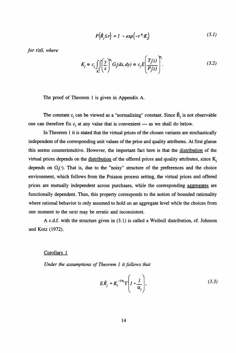
for r>.0, where

P(15_r) =1 - exp(-r a, K)

(3.1)

K. LS' CJ

X*7-1 G(dx, dy) ciE

J j

(3.2)

The proof of Theorem 1 is given in Appendix A.

The constant cj can be viewed as a "normalizing" constant. Since ki is not observable

one can therefore fix ci at any value that is convenient — as we shall do below.

In Theorem 1 it is stated that the virtual prices of the chosen variants are stochastically

independent of the corresponding unit values of the price and quality attributes. At first glanse

this seems counterintuitive. However, the important fact here is that the distribution of the

virtual prices depends on the distribution of the offered prices and quality attributes, since KJ

depends on Gio. That is, due to the "noisy" structure of the preferences and the choice

environment, which follows from the Poisson process setting, the virtual prices and offered

prices are mutually independent across purchases, while the corresponding aggregates are

functionally dependent. Thus, this property corresponds to the notion of bounded rationality

where rational behavior is only assumed to hold on an aggregate level while the choices from

one moment to the next may be erratic and inconsistent.

A c.d.f. with the structure given in (3.1) is called a Weibull distribution, cf. Johnson

and Kotz (1972).

Corollary 1

Under the assumptions of Theorem I it follows that

IC -"aT (3.3)

14

(3.7)Vark.

1= .

(Eki)2

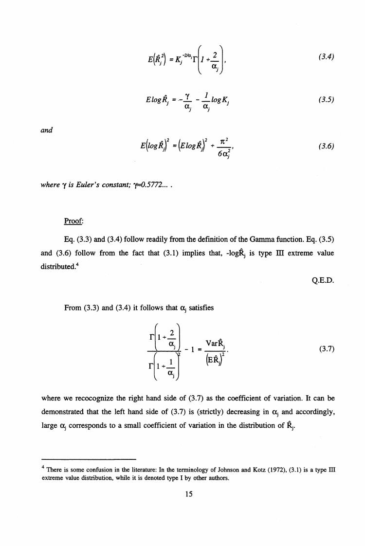
k 2= KJ -2 t / +--a.

'

ElogI = - 1 logK.a

.1. a. )

and

0°002 41°002 Tc2 (3.6)6a.f

where y is Euler's constant; .

Proof:

Eq. (3.3) and (3.4) follow readily from the definition of the Gamma function. Eq. (3.5)

and (3.6) follow from the fact that (3.1) implies that, -logki is type III extreme value

distributed.4

Q.E.D.

From (3.3) and (3.4) it follows that ai satisfies

(3.4)

(3.5)

where we recocognize the right hand side of (3.7) as the coefficient of variation. It can be

demonstrated that the left hand side of (3.7) is (strictly) decreasing in ai and accordingly,

large al corresponds to a small coefficient of variation in the distribution of

4 There is some confusion in the literature: In the terminology of Johnson and Kotz (1972), (3.1 ) is a type IIIextreme value distribution, while it is denoted type I by other authors.

15

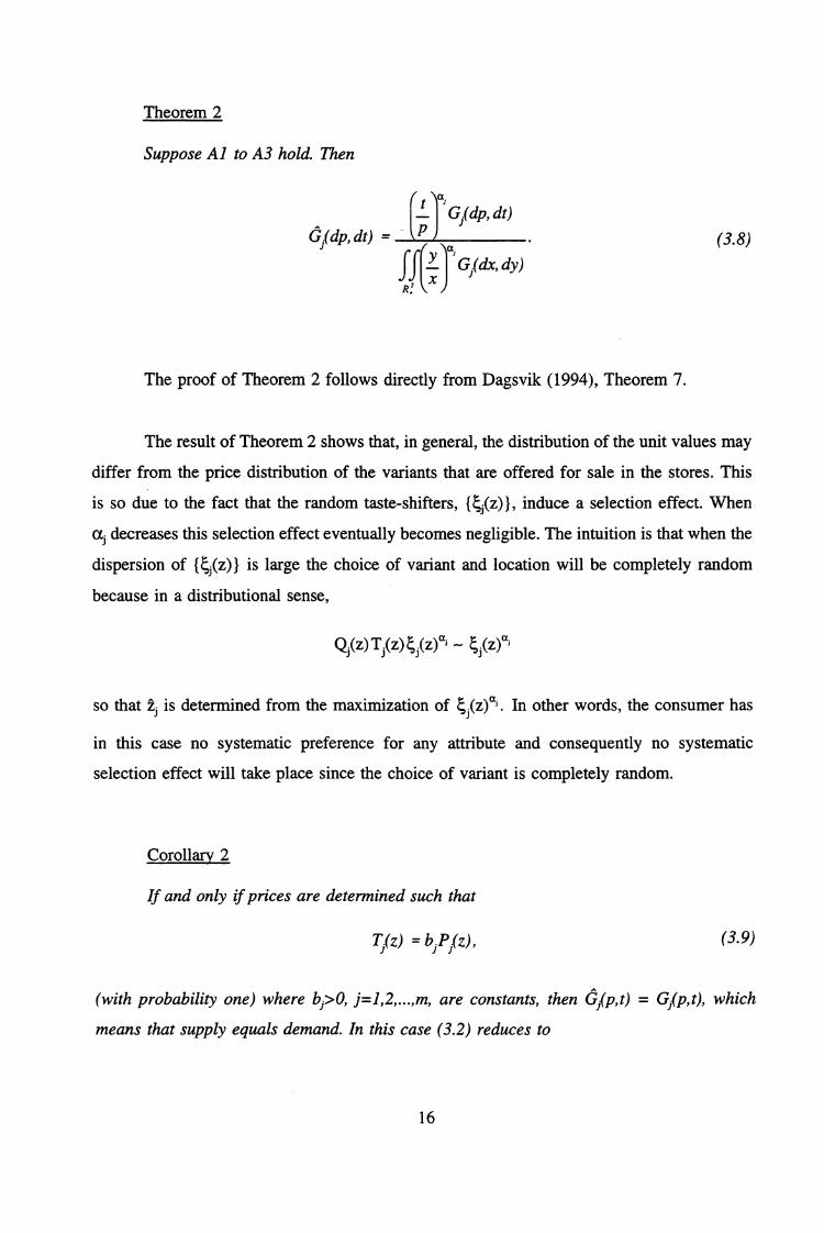
Theorem 2

Suppose Al to A3 hold. Then

j(dp, dt) = P

15(2-7,) G fdx, dy)x

a

Gi(dp, dt)

(3.8)

The proof of Theorem 2 follows directly from Dagsvik (1994), Theorem 7.

The result of Theorem 2 shows that, in general, the distribution of the unit values may

differ from the price distribution of the variants that are offered for sale in the stores. This

is so due to the fact that the random taste-shifters, { ti(z)}, induce a selection effect. When

ai decreases this selection effect eventually becomes negligible. The intuition is that when the

dispersion of {ti(z)} is large the choice of variant and location will be completely random

because in a distributional sense,

Qj(z)Tj(z)ti(z)a,

so that ; is determined from the maximization of ti(z)a' . In other words, the consumer has

in this case no systematic preference for any attribute and consequently no systematic

selection effect will take place since the choice of variant is completely random.

Corollary 2

If and only if prices are determined such that

Ti(z) = biPi(z), (3.9)

(with probability one) where b3>0, j=1,2,...,m, are constants, then 61p,t) = Glp,t), which

means that supply equals demand. In this case (3.2) reduces to

16

K. =.1 .1 •

(3.10)

Proof:

Assumption (3.9) means that Gi(dp10=1, when t/bj E (p,p+dp) and zero otherwise,

where Gi(plt) is the conditional distribution of prices in category j given that Ti(z)=.4. From

Theorem 2 and Theorem 1 the result of Corollary 2 follows.

Q.E.D.

If both prices, Ti-attributes as well as unit values and chosen attributes, { (f)i,t) }, were

observed then (3.8) could be utilized to estimate aj without additional assumptions about

gj •). Moreover, one could test the utility specification indirectly by testing the particular

functional form of (3.8) on the basis of non-parametric estimates of qo and 4().Unfortunately, the quality attributes are rarely observable and accordingly (3.8) is not readily

applicable for empirical analyses. To this end the next result is useful.

Corollary 3

Let

X.i(p) E(7;(z)a) I Piz) (3.11)

and assume that the density, gip), of the marginal price distribution exists. Eq. (3.8) implies

that the marginal density of unit values can be expressed as

-05 2‘• (n n.

VP) = Jr1611"

jf:

x -a, 2(x) gi(x)dx(3.12)

Moreover,

17

K. = c.fx -a, X.(x)g.(x)dx.JJ JJ

R .

(3.13)

The result of Corollary 3 demonstrates that when {T i(z)} is unobservable then a most p Xj(p)

can be identified from the relationship between the respective distribution of prices and unit

values.

Proof:

By (3.8) we can express gi(p) as

p -aig1)) =

g(p) E(Tj(z)ai Pi(z) =p-(

fx -ai gi(x) E(Ti(z)ai I Pi(z) = dxR,

Eq. (3.12) now follows immediately and (3.13) follows from (3.2).

Q.E.D.

The function A.,i() is in fact a (preference-adjusted) conditional aggregate quality ,

index. Specifically, 2t.,j(p) expresses the conditional mean value across variants of the

quality/location attributes given price level p. It is adjusted for heterogeneity in tastes through

the parameter a. In general it is desirable to link 2Li(p) to observable attributes of the product

variants. For simplicity, we shall defer the introduction of observable nonpecuniary attributes

till Section 6. From the discussion there it will become evident that the approach in Section

6 also applies to the present case with divisible products.

From Corollary 3 the next result is immediate.

18

Corollary 4

If

*pa' IP(z) =P) w (3.14)

where w3>0 is a constant, then by (3.12) the distribution of unit values equals the distribution

of prices.

Note, however, that ki(p) = gi(p) does not necessarily mean that the equilibirum

condition, ki(p,t) = gi(p,t) holds, cf. Corollary 2.

Corollary 5

The parameter Ki of the virtual price distribution can be expressed as

cE(T (z)a)K. c,E _ . , J.1 piz) jT iz) = c..E(Plz)-aiXJ(Plz))) = (^ a)E P.J

1 1 -1 = / EJ

(3.15)

Moreover,

(3.16)

Proof:

The first and second equality of (3.15) follow from (3.2) and (3.13). From (3.12) we

Kj g;(1))P = Op) ci2■,;(p)

(3.17)

get

19

which implies that

K. fx aj k'.(x) dx K. E(15 .ai) = c. fk.(x) g.(x) dx c. E (Pi(z))) = ci E T.(z)ajJ J J J J J J J k J

R.

3.18)

and

X ai g .( x) dx.f J = K E

A(x)J (3.19)

J )

and thus the last equality in (3.15) has been proved. Also (3.16) follows from (3.17) and

(3.18).

Q.E.D.

Corollary 5 demonstrates that once aj and Xi() have been estimated it is sufficient to

have observations on unit values to obtain an estimate of N.Although it is not of primary focus in this paper the results concerning the c.d.f. of

virtual prices can be applied to obtain price indexes. From Theorem 1, Corollary 2 and

Corollary 5 it follows that ilc" can be interpreted as a price index. By (3.15) we can

express this price index as

-1/a ( JJ

KR

A(x) g(x) dxJ J J J J

•

(3.20)

where ci can be chosen so as to adjust the level of the index to be equal to the corresponding

price level in a reference year. In contrast to the conventional price indexes, (3.20) is in fact

a price index functional, since is depends on the whole probability distribution of prices.

A fundamental question is to which extent we can identify the distribution of the

virtual prices and the corresponding demand system.

20

P -°52;(13) = X.i(1) gi(p) gi(1)

gi(p)fti(1)

Corollary 6

Assume that (p) and gip) are known. Under the assumptions of Theorem i it follows

that p --c5 k.(p) is non-parametrically identified apart from a multiplicative constant.

Proof:

From (3.12) we get

which yields the above results.

Q.E.D.

We found above that i(p)p -a, is only identified up to a multiplicative constant.

Unless we impose additional structure on X(p) or on the corresponding utility function

introduced in Al we cannot pursue this matter further. We shall next introduce an additional

assumption and examine the implications thereof.

Assumption A4

For each commodity group j,

?L(p) *Pa' 'Piz) =PaiKiE(Tiz)a)

(3.21)E(Pj(z)al

where Ki is a constant (possible time dependent).

Before we discuss the interpretation of A4 we state an immediate result.

21

Corollary 7

Under A4, (3.12) and (3.13) reduce to

a .x. -a. )p Tip

CCAg j( x) dx

(3.22)

and

T( z)1 EKi = cj

E(P/Z)al(3.23)

Under Assumption A4 it follows that

a2 E(rj(z)cs 1 1);(z)Œi =3') (ici -1) y 2 E (T;(z)1 a y 2

E(Pj(z) )

Consequently, under A4 the function X.6,111 is convex when Kj>1 and concave when K. 1J l<

The interpretation is that when Kj<1, then the dependence between Ti( ) and Pi(z)a, is

weakened when the price level increases, while when ici>1 this dependence is strenghtened

when the price level increases. The latter case means that price is perceived as an increasingly

more "reliable" proxy for quality as the price level increases. Without real loss of generality,

suppose now that the probability mass of prices less than one is negligible. From (3.22) we

realize that Kj<1 implies that ki(p) is more skew to the left than gi(p), while the opposite is

true when K>1. The reason is of course that when Kj>l, increasing prices do not reduce the

attractiveness of the product variants as much as when because high prices are perceived

as a strong indication of high quality, and vice versa.

As regards identification, Assumption A4 is not sufficient to fully resolve the issue

unless we are willing to make assumptions about how E(Ti(z)1 j=1,2,...,m, changes over

time (cf. (3.23)).

22

4. A special case: AIDS demand system

Let wj, denote the budget share of type j for a particular consumer in period 't and

let {k}, {Pit(z)} and {Pit } be the corresponding virtual prices, prices and unit values. Now

assume that the appropriate demand system is an AIDS model given by

= hj E B iklogk + fl i log(y,/qt)k

and

log + E hk logRk^ !E Ej=1 S jk log R., logk

111

where y, is total expenditure for the consumer in period T, {f3j }, {hk } and {8ik ) are unknown

parameters which satisfy

J = 1, 8 jk 8 kj

and

E 8 1 = E 8 - "-= E 13 - = 05k j

(cf. Deaton and Muellbauer, 1980). For simplicity, we rule out the possibility of corner

solutions. By Corollary 1 we have

(4.1)

(4.2)

Ew. = h. -it J A-. 5 i

k=1

(

ak

N1- log Kkr ß j Elogy i, P j Elogqi,ak

(4.3)

where

E log cir - E hk

k=1

+ _1 log Kk,

ak akjk2 k= 1 j= 1

(4.4)(

+ - log K., + 1 logKk,7 1oc. oc. al oc ocJ J A k k

23

and y=0.5772..., is Euler's constant. Provided one is willing to assume that E Tit( )1 is

constant over time, there is no loss of generality in assuming that

ciE(Tit(z)ai) = 1

which by (3.15) imply that

itlog Kit = -logE )• ai

The identification and estimation of this — and the linear expenditure system will be

discussed in Part II of this paper.

The analysis in this section can, as mentioned above, easily be extended to the case

in which nonpecuniary attributes are present. We refer to the next section for details about

this extension.

5. Discrete choice

In the context of qualitative choice — such as the demand for durables, choice among

jobs and schooling decisions — the set of feasible alternatives is typically discrete. Berry et

al. (1995) have developed a discrete choice technique to analyze demand with latent quality

attributes. Their approach differs from the one described below in that Berry et al. assume

that the classification of product variants relevant to the consumers is observable. In addition,

their assumptions about the stochastic elements of the model differ from the assumptions

invoked here.

In this section we shall modify the analysis above so as to apply in the discrete choice

setting in which the consumer only purchases one unit of a product variant at a time. Thus

the vector of quantities, Q, has components that are either zero or one.

Specifically, we now assume the following:

(4.5)

(4.6)

24

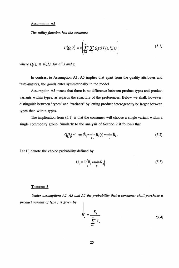
Assumption A5

The utility function has the structure

u(Q, =u[E z Q(z)Tlz) (z)

where Qj(z) E (0,. 1], for all j and z.

In contrast to Assumption Al, A5 implies that apart from the quality attributes and

taste-shifters, the goods enter symmetrically in the model.

Assumption A5 means that there is no difference between product types and product

variants within types, as regards the structure of the preferences. Below we shall, however,

distinguish between "types" and "variants" by letting product heterogeneity be larger between

types than within types.

The implication from (5.1) is that the consumer will choose a single variant within a

single commodity group. Similarly to the analysis of Section 2 it follows that

Q(î) = i 4=> ki =min Rk(r) = min ftkk,r k

Let H denote the choice probability defined by

H. P R. =minkkk

Theorem 3

Under assumptions A2, A3 and AS the probability that a consumer shall purchase a

product variant of type j is given by

K.H =

J

E Kr

(5.1)

(5.2)

(5.3)

(5.4)

25

Proof:

Let yi -ailoglkj . From (3.1) it follows that Vi has c.d.f.

= P(Iki >e = exp(-e (5.5)

But this means that yi logKj + Ili , where 11012,...,im, are independent with extreme value

c.d.f., exp( -e-Y). But then (5.4) follows immediately from a familiar result in discrete choice

theory (cf. Ben-Akiva and Lerman, 1985), because minimization of I is equivalent to

maximization of

Q.E.D.

In many fields of discrete choice, such as choice of housing, residential location,

tourist destinations, etc., the consumer faces many product variants of each type, and it is

often the case that in addition to prices, nonpecuniary attributes associated with the chosen

variants are observable to the analyst. We shall now extend the framework developed above

to take into account observable attributes that characterize the variants. Let X(z) denote the

observable nonpecuniary attribute (possible vector-valued) associated with variant z of type

J.

To focus on the potential for empirical applications we shall express the choice

probabilities under additional assumptions about the distribution of {Ti(z)}.

Assumption A6

The vectors in id [(Plz),7iz),Xlz),(z)), j=1,2,...,m, are points of

independent inhomogeneous Poisson processes on R+3 xRxR, with intensity measure associated

with pi equal to

G .(dp, dt clx) e -II, c .de , (5.6)

where ocj>0, c3>0.

Clearly, A6 is an immediate extension of A2 and A3.

26

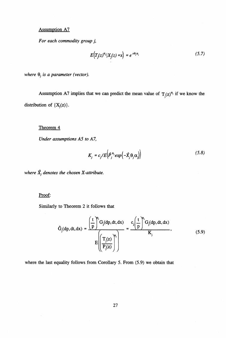
Assumption A7

For each commodity group j,

Efri(z)a, Wiz) =x) = e x

(5.7)

where Oj is a parameter (vector).

Assumption A7 implies that we can predict the mean value of Ti(z)a, if we know the

distribution of { Xj(z) } .

Theorem 4

Under assumptions A5 to A7,

C i/E 15;5 exp(A0i(5.8)

where if denotes the chosen X-attribute.

Proof:

Similarly to Theorem 2 it follows that

6j(dp, dt. dx)Gi(dp, dt. dx)

(5.9)

where the last equality follows from Corollary 5. From 5.9 we obtain that

27

p aidtdx) = c. t ai G (dp, dt, dx)

, Ki

(5.10)

which together with A7 implies that

E(Piaiexp(-kj O. oci)) = EE(Pia'exp(-ki ej ai) I ki)

j E (exp ( -Xj(z) 0 E (zT. )cs X.(z)= E (exp ( -kJ ei ai) E (f) icS lkj)) =

cJ

Ki K. .J

Q.E.D.

Theorems 3 and 4 suggest that it may be possible to estimate faj l and { ej } solely

from observations on unit values and chosen X-attributes without imposing restrictions on the

conditional moment, Efri(z)ai IPj(z),Xj(z)). However, for the purpose of analyzing the effect

from a change in the distribution of prices and nonpecuniary attributes, it is necessary also

to make assumptions about the conditional moment. A direct extension from Assumption A4

would be to make the following assumption:

Assumption A8

For each commodity group j,

E(7iejlPj(z) =p, X3(z) =xcc.x.p

E(P Zr(5.11)

where ej and Ki are parameters.

From Assumption A8 it follows that we can express Ki as

28

K.(x) c.EJ J

f( ■05

T J.(z)I Xi(z) = x

P.(z)

(5.14)

E (1) .(z)ai lci exp(X :(z) O. a.))K. J J D

JE(Pi(z)csKi)

(5.12)

Let us finally consider the relevance of the present setup for the theory and estimation

of hedonic price indexes. Recall from the discussion following Theorem 1 that within the

Poisson process framework proposed in this paper, dependence between virtual prices and

attributes and prices must be understood in a "distributional sense". Consequently, we shall

interpret the hedonic price index as the mean virtual price when the set of feasible attributes

and prices are generated by the conditional distributions, Gi(p,t1x), given x, j=1,2,...,m. The

corresponding virtual price distributions (cf. Theorem 1) thus take the form

P (ki(x) = 1 - exp (-r ai Ki(X))

(5.13)

where

Similarly to (3.3) we get

Efki(x) = K.(x) -uaiFJ

(5.15)

We shall interpret (5.15) as our hedonic price index. Recall that Eki may also be interpreted

as a price index. To distinguish the two price index definitions we may call Eki(x) and EP.i

the conditional and unconditional hedonic price indexes, respectively. While Eki(x) depends

on the conditional distribution of offered prices given level x of the nonpecuniary attributes,

Eki depends on the unconditional distribution of offered prices and attributes.

When Assumption A8 holds we get immediately from (5.14) and (5.10) that

29

_1/a,

E(Pj(z)ai ls)

_ci E(Pi(z)ai )s -ai)

(r 1 =e

a.Eft(x) = e

-1/ar+,

__ •Cia.I

1/a, (5.16)

6. Conclusions

When consumer goods differ by quality and location, traditional demand analysis is

no longer appropriate. In this paper we have demonstrated that by means of a particular

probabilistic framework for discrete and continuous choice, it is possible to modify standard

consumer theory to accommodate a rather general environment with a rich variety of product

variants with product characteristics that may partly be unobservable to the analyst.

Finally, we present the corresponding analysis for the case of demand for indivisible

goods of which some of the attributes may be observable and we also outline how hedonic

price indexes can be established.

30

Appendix A

Lemma 1

Suppose that A2 holds and that

E,

fi.i.(e)dE = 0.c,10 j

Then with probability one there exists a point z in pjfor which (Plz),Ti(z)E A), where A is an

arbitrary open Borel set in le

Proof:

Recall first that if A is a Borel set in R.2, the probability density of the number of

points within A A x [e 1 ,e2], Ni(Ä), for e i<E2, is given by

Kik n

13 (1\1j(Ä.- ) =11) exp(-1\40n!

where

M(Ã) = fGi(dp,dt) pi(E) de .

Hence, it follows that for A = [p,p+dp] x [t,t+dt] we get

(

P(NjCik )>. 1) = i - exp

£2

- Gi(dp,dt) fl.tj(E) deE,

Now suppose that 1.1j has the property that

£2

lim de ---400 .

31

Then it follows that P(Ni(Ä)>A) converges towards one as e l -> O.

Q.E.D.

Proof of Theorem 1:

Recall that (15i,t) is defined by Pi=Pi(;), ti=Tj(2) where

( (T(z)

2. a= rgmaxz a.log j

J J P(z)\

(A.1)

where 4;(z)=ailogj(z). Let A be a Borel set in R2. and define

f

1,j(A) = maxi ai log(p,(z), Ti(z)) e A

(T :(z)

J +4;(z)P.(z)\ J j

(A.2)

and

)L.(A = maxi ai logJ(1),(z),Ti(z))e A \

Tj(z)

P.(z)-1 I

(A.3)

It follows that Li(A) and Li(A) are stochastically independent because maximum is taken over-

Poisson points in disjoint sets, A and A. Moreover, it can be demonstrated that Li(A) and

L(A) are extreme value distributed (type 111) i.e.

P(Li(C)...x) = exp(-Di(C)e -x)

for C equal to A and A, respectively, where

D i(C) = cv

. g(j ,x,y) dx dy.

, xkx,y)ec

(See Dagsvik (1994), for a proof of this.) We have

(A.4)

(A.5)

32

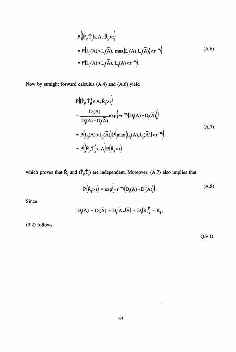
P ((15j, ti) E A, kj

= 141,j(A)>Li(A-.), max(Li(A),Lj A -a,

= P(Li(A)>Lj(A),_Li(A)<r

Now by straight forward calculus (A.4) and (A.6) yield

P ((f)j, ti) E A, kj >

Dj(A) exp(-r --°`'ODi A Di ADi(A) +Di(A)

= P(Li(A)>Li(A .))P(max(Li(A),Li(A1))

= P ti) E P >r)

which proves that Ñ. and (f,î') are independent. Moreover, (A.7) also implies that

P(!>r) = exp(- -a, (Dj(A) +Dj( ))).

Since

D.(A) + Di(Ä) = NAUÄ) = Di (R+2) =

(3.2) follows.

(A.6)

(A.7)

A.8)

Q.E.D.

33

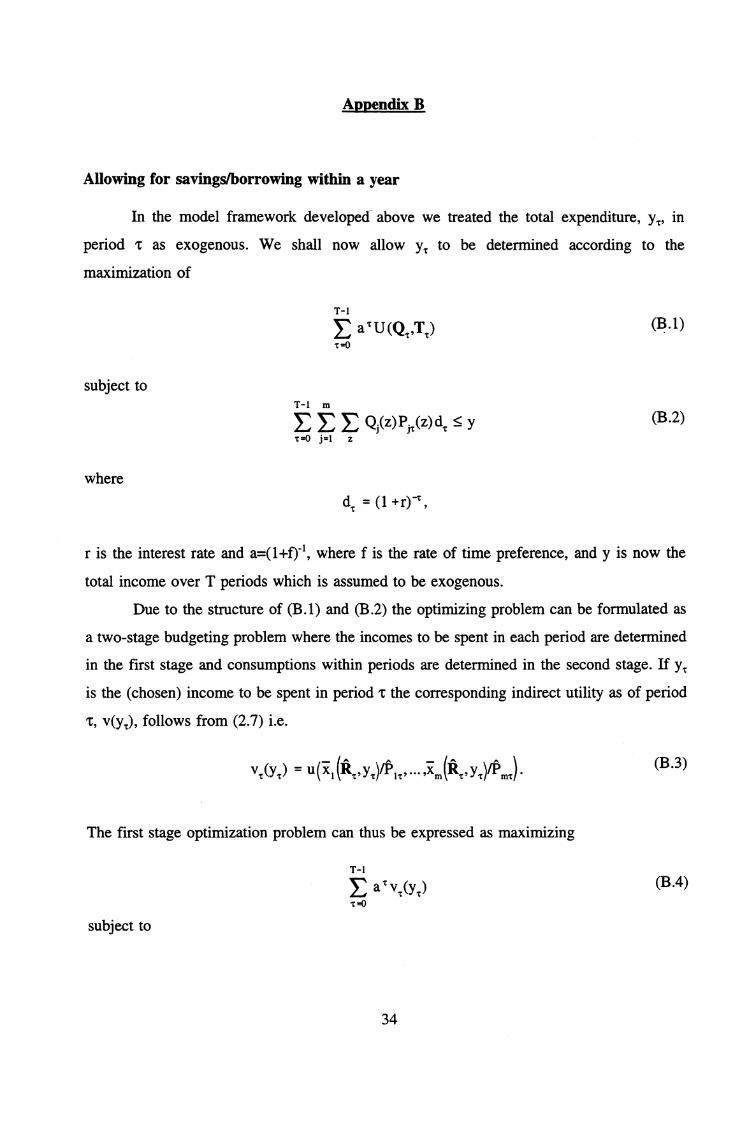
Appendix B

Allowing for savings/borrowing within a year

In the model framework developed above we treated the total expenditure, yt, in

period 't as exogenous. We shall now allow yt to be determined according to the

maximization of

T-1

E a T U(Q,,T)v=o

subject toT-1 m

E EE Q;(z)pit(z)dt y;=, z

(B.2)

where

d, = (1 +r)',

r is the interest rate and a=(1+0-1 , where f is the rate of time preference, and y is now the

total income over T periods which is assumed to be exogenous.

Due to the structure of (B.1) and (B.2) the optimizing problem can be formulated as

a two-stage budgeting problem where the incomes to be spent in each period are determined

in the first stage and consumptions within periods are determined in the second stage. If yt

is the (chosen) income to be spent in period it the corresponding indirect utility as of period

v(y), follows from (2.7) i.e.

v(y) = u (11,, y„)/P i , ytytemT) .

The first stage optimization problem can thus be expressed as maximizing

T-1

E a 't vt(yt)

subject to

(B.3)

(B.4)

34

yd (8.5)

In the case where the demand system has the structure (5.1) it follows that the period-

specific indirect utility is given by

\

[m m

v(y) = log yt -E yi ki, - E f3 logÑ.i=1 j j=1

(B.6)

From (B.4), (8.5) and (B.6) it follows readily that the corresponding first stage solution is

given by

T-1

E

(

T-1 m

a 't y-E d E 1 -a)k 'j R kj=1

(1a T)d,,

In the particular case when r=0 and a=1, (B.7) reduces to

(

1 1

(B.7)

= EJ .1 '

T-1 m

-E Ek=0 j=1

(B.8)jk

35

References

Anderson, S.P., A. de Palma and J.F. Thisse (1992): Discrete Choice Theory of ProductDifferentiation. MIT Press, Cambridge.

Bartik, T.J. (1987): The Estimation of Demand Parameters in Hedonic Price Models. Journalof Political Economy, 95, 81-88.

Ben-Akiva, M. and S.R. Lerman (1985): Discrete Choice Analysis. MIT Press, Cambridge.

Berry, S. J.A. Levinsohn and A. Pakes (1995): Automobile Prices in Market Equilibrium.Econometrica, 63, 841-890.

Brown, J.N. and H.S. Rosen (1982): On the Estimation of Structural Hedonic Price Models.Econometrica, 55, 765-768.

Chamberlin, E.H. (1933): The Theory of Monopolistic Competition. Harvard University Press,Cambridge.

Dagsvik, J.K. (1994): Discrete and Continuous Choice, Max-stable Processes andIndependence from Irrelevant Attributes. Econometrica, 62, 1179-1205.

Dagsvik, J.K. (1995): Consumer Demand with Unobservable Product Attributes. Part II:Inference. Discussion Paper, Statistics Norway.

Deaton, A. (1987): Estimation of Own- and Cross-Price Elasticities from Household SurveyData. Journal of Econometrics, 36, 7-30.

Deaton, A. (1988): Quality, Quantity, and Spatial Variation of Price. American EconomicReview, 78, 418-430.

Deaton, A.S. and J. Muellbauer (1980): An Almost Ideal Demand System. AmericanEconomic Review, 70, 312-336.

Dixit, A., and J.E. Stiglitz (1977): Monopolistic Competition and Optimum Product Diversity.Journal of Political Economy, 74, 221-237.

Epple, D. (1987): Hedonic Prices and Implicit Markets: Estimating Demand and SupplyFunctions for Differentiated Products. Journal of Political Economy, 95, 59-80.

Fisher, F.M. and K. Shell (1971): Taste and Quality Change in the Pure Theory of the TrueCost of Living Index. In Z. Griliches (eds.), Price Indexes and Quality Changes: Studies Inthe New Methods of Measurement. Harvard University Press, Cambridge.

Gorman, W.M. (1976): Tricks with Utility Functions. In M. Artis and R. Nobay (eds.), Essaysin Economic Analysis, Cambridge University Press, Cambridge.

36

Haneman, W.M. (1984): Discrete/Continuous Choice of Consumer Demand. Econometrica,52, 541-561.

Houthakker, H.S. and S.J. Prais (1952): Les Variations de Qualité dans les Budgets deFamille. Economie Appliquée, 5, 65-78.

Houthakker, H.S. and S.J. Prais (1955): - The Analysis of Family Budgets. CambridgeUniversity Press, New York.

Johnson, N.L. and S. Kotz (1972): Distributions in Statistics: Continuous UnivariateDistributions. Wiley, New York.

Krugman, P. (1989): Industrial Organization and International Trade. In R. Schmalensee andR.D. Willig (eds.), Handbook of Industrial Organization, Vol. II, Elsevier Science Publishers,Amsterdam.

Lancaster, K.J. (1966): A New Approach to Consumer Theory. Journal of Political Economy,74, 132-157.

Lancaster, K. (1977): The Measurement of Changes in Quality. Review of Income and Wealth,23, 157-172.

Lancaster, K.J. (1979): Variety, Equity and Efficiency. Columbia University Press, New Yak

Muellbauer, J. (1974): Household Production Theory, Quality, and the "Hedonic Technique".American Economic Review, 64, 977-994.

Rosen, S. (1974): Hedonic Prices and Implicit Markets: Product Differentiation in PureCompetition. Journal of Political Economy, 82, 35-55.

Spence, M.E. (1976): Product Selection, Fixed Costs, and Monopolistic Competition. Rev.Economic Studies, 43, 217-236.

Stiglitz, J.E. (1987): The Causes and Consequences of the Dependence of Quality on Price.Journal of Economic Literature, 25, 1-48.

Trajtenberg, M. (1989): Product Innovations, Price Indices and (Miss)Measurement ofEconomic Performance. Working Paper, 26-89, Foerder Institute for Economic Research, TelAviv.

37

Issued in the series Discussion Papers

42 R. Aaberge, O. Kravdal and T. Wennemo (1989): Un-observed Heterogeneity in Models of Marriage Dis-solution.

43 K.A. Mork, H.T. Mysen and O. Olsen (1989): BusinessCycles and Oil Price Fluctuations: Some evidence for six-OECD countries.

44 B. Bye, T. Bye and L. Lorentsen (1989): SIMEN. Studiesof Industry, Environment and Energy towards 2000.

45 0. Bjerkholt, E. Gjelsvik and O. Olsen (1989): GasTrade and Demand in Northwest Europe: Regulation,Bargaining and Competition.

46 L.S. Stambøl and K.O. Sorensen (1989): MigrationAnalysis and Regional Population Projections.

47

V. Christiansen (1990): A Note on the Short Run VersusLong Run Welfare Gain from a Tax Reform.

48 S. Glomsrød, H. Vennemo and T. Johnsen (1990): Sta-bilization of Emissions of CO2: A Computable GeneralEquilibrium Assessment.

49 J. Aasness (1990): Properties of Demand Functions forLinear Consumption Aggregates.

50 J.G. de Leon (1990): Empirical EDA Models to Fit andProject Time Series of Age-Specific Mortality Rates.

51 J.G. de Leon (1990): Recent Developments in ParityProgression Intensities in Norway. An Analysis Based onPopulation Register Data

52 R. Aaberge and T. Wennemo (1990): Non-StationaryInflow and Duration of Unemployment

53 R. Aaberge, J.K. Dagsvik and S. Strom (1990): LaborSupply, Income Distribution and Excess Burden ofPersonal Income Taxation in Sweden

54 R. Aaberge, J.K. Dagsvik and S. Strøm (1990): LaborSupply, Income Distribution and Excess Burden ofPersonal Income Taxation in Norway

55 H. Vennemo (1990): Optimal Taxation in Applied Ge-neral Equilibrium Models Adopting the ArmingtonAssumption

56 N.M. Stolen (1990): Is there a NAIRU in Norway?

57 A. Cappelen (1991): Macroeconomic Modelling: TheNorwegian Experience

58 J.K. Dagsvik and R. Aaberge (1991): HouseholdProduction, Consumption and Time Allocation in Peru

59

R. Aaberge and J.K. Dagsvik (1991): Inequality inDistribution of Hours of Work and Consumption in Peru

60 T.J. Klette (1991): On the Importance of R&D andOwnership for Productivity Growth. Evidence fromNorwegian Micro-Data 1976-85

61 K.H. Alfsen (1991): Use of Macroeconomic Models inAnalysis of Environmental Problems in Norway andConsequences for Environmental Statistics

62 H. Vennemo (1991): An Applied General EquilibriumAssessment of the Marginal Cost of Public Funds inNorway

63 H. Vennemo (1991): The Marginal Cost of PublicFunds: A Comment on the Literature

64 A. Brendemoen and H. Vennemo (1991): A climateconvention and the Norwegian economy: A CGE as-sessment

65 K.A. Brekke (1991): Net National Product as a WelfareIndicator

66 E. Bowitz and E. Storm (1991): Will Restrictive DemandPolicy Improve Public Sector Balance?

67 A. Cappelen (1991): MODAG. A Medium TermMacroeconomic Model of the Norwegian Economy

68 B. Bye (1992): Modelling Consumers' Energy Demand

69 K.H. Alfsen, A. Brendemoen and S. Glomsrød (1992):Benefits of Climate Policies: Some Tentative Calcula-tions

70 R. Aaberge, Xiaojie Chen, Jing Li and Xuezeng Li(1992): The Structure of Economic Inequality amongHouseholds Living in Urban Sichuan and Liaoning,1990

71 K.H. Alfsen, K.A. Brekke, F. Brunvoll, H. Lurås, K.Nyborg and H.W. Sæbø (1992): Environmental Indi-cators

72 B. Bye and E. Holmøy (1992): Dynamic EquilibriumAdjustments to a Terms of Trade Disturbance

73 0. Aukrust (1992): The Scandinavian Contribution toNational Accounting

74 J. Aasness, E. Eide and T. Skjerpen (1992): A Crimi-nometric Study Using Panel Data and Latent Variables

75 R. Aaberge and Xuezeng Li (1992): The Trend inIncome Inequality in Urban Sichuan and Liaoning, 1986-1990

76 J.K. Dagsvik and S. Strom (1992): Labor Supply withNon-convex Budget Sets, Hours Restriction and Non-pecuniary Job-attributes

77 J.K. Dagsvik (1992): Intertemporal Discrete Choice,Random Tastes and Functional Form

78 H. Vennemo (1993): Tax Reforms when Utility isComposed of Additive Functions

79 J.K. Dagsvik (1993): Discrete and Continuous Choice,Max-stable Processes and Independence from IrrelevantAttributes

80 J.K. Dagsvik (1993): How Large is the Class of Gen-eralized Extreme Value Random Utility Models?

81 H. Birkelund, E. Gjelsvik, M. Aaserud (1993): Carbon/energy Taxes and the Energy Market in WesternEurope

82 E. Bowitz (1993): Unemployment and the Growth in theNumber of Recipients of Disability Benefits in Norway

83 L. Andreassen (1993): Theoretical and EconometricModeling of Disequilibrium

84 K.A. Brekke (1993): Do Cost-Benefit Analyses favourEnvironmentalists?

85 L. Andreassen (1993): Demographic Forecasting with aDynamic Stochastic Microsimulation Model

86 G.B. Asheitn and K.A. Brekke (1993): Sustainabilitywhen Resource Management has Stochastic Conse-quences

87 0. Bjerkholt and Yu Zhu (1993): Living Conditions ofUrban Chinese Households around 1990

88 R. Aaberge (1993): Theoretical Foundations of LorenzCurve Orderings

89 J. Aasness, E. Morn and T. Skjerpen (1993): EngelFunctions, Panel Data, and Latent Variables - withDetailed Results

38

90 I. Svendsen (1993): Testing the Rational ExpectationsHypothesis Using Norwegian Microeconomic DataTesting the REH. Using Norwegian MicroeconomicData

91 E. Bowitz, A. Rødseth and E. Storm (1993): FiscalExpansion, the Budget Deficit and the Economy: Nor-way 1988-91

92 R. Aaberge, U. Colombino and S. Strøm (1993): LaborSupply in Italy

93 T.J. Klette (1993): Is Price Equal to Marginal Costs? AnIntegrated Study of Price-Cost Margins and ScaleEconomies among Norwegian Manufacturing Estab-lishments 1975-90

94 J.K. Dagsvik (1993): Choice Probabilities and Equili-brium Conditions in a Matching Market with FlexibleContracts

95 T. Kornstad (1993): Empirical Approaches for Ana-lysing Consumption and Labour Supply in a Life CyclePerspective

96 T. Kornstad (1993): An Empirical Life Cycle Model ofSavings, Labour Supply and Consumption withoutIntertemporal Separability

97 S. Kvemdokk (1993): Coalitions and Side Payments inInternational CO2 Treaties

98 T. Eika (1993): Wage Equations in Macro Models.Phillips Curve versus Error Correction Model Deter-mination of Wages in Large-Scale UK Macro Models

99 A. Brendemoen and H. Vennemo (1993): The MarginalCost of Funds in the Presence of External Effects

100 K.-G. Lindquist (1993): Empirical Modelling ofNorwegian Exports: A Disaggregated Approach

101 A.S. Jorn, T. Skjerpen and A. Rygh Swensen (1993):Testing for Purchasing Power Parity and Interest RateParities on Norwegian Data

102 R. Nesbaldcen and S. Strøm (1993): The Choice of SpaceHeating System and Energy Consumption in NorwegianHouseholds (Will be issued later)

103 A. Aaheim and K. Nyborg (1993): "Green NationalProduct": Good Intentions, Poor Device?

104 K.H. Alfsen, H. Birkelund and M. Aaserud (1993):Secondary benefits of the EC Carbon/ Energy Tax

105 J. Aasness and B. Holtsmark (1993): Consumer Demandin a General Equilibrium Model for EnvironmentalAnalysis

106 K.-G. Lindquist (1993): The Existence of Factor Sub-stitution in the Primary Aluminium Industry: A Multi-variate Error Correction Approach on Norwegian PanelData

107 S. Kverndokk (1994): Depletion of Fossil Fuels and theImpacts of Global Warming

108 K.A. Magnussen (1994): Precautionary Saving and Old-Age Pensions

109 F. Johansen (1994): Investment and Financial Con-straints: An Empirical Analysis of Norwegian Firms

110 K.A. Brekke and P. Boring (1994): The Volatility of OilWealth under Uncertainty about Parameter Values

111 Mi. Simpson (1994): Foreign Control and NorwegianManufacturing Performance

112 Y. Willassen and Ti. Klette (1994): CorrelatedMeasurement Errors, Bound on Parameters, and a Modelof Producer Behavior

113 D. Wetterwald (1994): Car ownership and private caruse. A microeconometric analysis based on Norwegiandata

114 K.E. Rosendahl (1994): Does Improved EnvironmentalPolicy Enhance Economic Growth? Endogenous GrowthTheory Applied to Developing Countries

115 L. Andreassen, D. Fredriksen and O. Ljones (1994): TheFuture Burden of Public Pension Benefits. AMicrosimulation Study

116 A. Brendemoen (1994): Car Ownership Decisions inNorwegian Households.

117 A. Langørgen (1994): A Macromodel of LocalGovernment Spending Behaviour in Norway

118 K.A. Brekke (1994): Utilitarism, Equivalence Scales andLogarithmic Utility

119 K.A. Brekke, H. Luis and K. Nyborg (1994): SufficientWelfare Indicators: Allowing Disagreement inEvaluations of Social Welfare

120 T.J. Klette (1994): R&D, Scope Economies and Com-pany Structure: A "Not-so-Fixed Effect" Model of PlantPerformance

121 Y. Willassen (1994): A Generalization of Hall's Speci-fication of the Consumption function

122 E. Holmoy, T. Hægeland and O. Olsen (1994): EffectiveRates of Assistance for Norwegian Industries

123 K. Mohn (1994): On Equity and Public Pricing inDeveloping Countries

124 J. Aasness, E. Eide and T. Skjerpen (1994): Crimi-nometrics, Latent Variables, Panel Data, and DifferentTypes of Crime

125 E. BiOrri and T.J. Klette (1994): Errors in Variables andPanel Data: The Labour Demand Response to PermanentChanges in Output

126 I. Svendsen (1994): Do Norwegian Firms FormExtrapolative Expectations?

127 T.J. Klette and Z. Griliches (1994): The Inconsistency ofCommon Scale Estimators when Output Prices areUnobserved and Endogenous

128 K.E. Rosendahl (1994): Carbon Taxes and the PetroleumWealth

129 S. Johansen and A. Rygh Swensen (1994): TestingRational Expectations in Vector Autoregressive Models

130 T.J. Klette (1994): Estimating Price-Cost Margins andScale Economies from a Panel of Microdata

131 L. A. Grünfeld (1994): Monetary Aspects of BusinessCycles in Norway: An Exploratory Study Based onHistorical Data

132 K.-G. Lindquist (1994): Testing for Market Power in theNorwegian Primary Aluminium Industry

133 T. J. Klette (1994): R&D, Spillovers and Performanceamong Heterogenous Firms. An Empirical Study UsingMicrodata

134 K.A. Brekke and H.A. Gravningsmyhr (1994): AdjustingNNP for instrumental or defensive expenditures. Ananalytical approach

135 T.O. Thoresen (1995): Distributional and BehaviouralEffects of Child Care Subsidies

136 T. J. Klette and A. Mathiassen (1995): Job Creation, JobDestruction and Plant Turnover in NorwegianManufacturing

137 K. Nyborg (1995): Project Evaluations and DecisionProcesses

138 L. Andreassen (1995): A Framework for EstimatingDisequilibrium Models with Many Markets

39

139 L. Andreassen (1995): Aggregation when Markets donot Clear

140 T. Skjerpen (1995): Is there a Business Cycle Com-ponent in Norwegian Macroeconomic Quarterly TimeSeries?

141 J.K. Dagsvik (1995): Probabilistic Choice Models forUncertain Outcomes

142 M. ROnsen (1995): Maternal employment in Norway, Aparity-specific analysis of the return to full-time andpart-time work after birth

143 A. Bruvoll, S. Glomsrod and H. Vennemo (1995): TheEnvironmental Drag on Long- term Economic Perfor-mance: Evidence from Norway

144 T. Bye and T. A. Johnsen (1995): Prospects for a Com-mon, Deregulated Nordic Electricity Market

145 B. Bye (1995): A Dynamic Equilibrium Analysis of aCarbon Tax

146 T. O. Thomsen (1995): The Distributional Impact of theNorwegian Tax Reform Measured by Disproportionality

147 E. Holm:1y and T. Hægeland (1995): Effective Rates ofAssistance for Norwegian Industries

148 J. Aasness, T. Bye and H.T. Mysen (1995): WelfareEffects of Emission Taxes in Norway

149 J. Aasness, E. BiOrn and Terje Skjerpen (1995):Distribution of Preferences and Measurement Errors in aDisaggregated Expenditure System

150 E. Bowitz, T. F3e11/1, L A. Grünfeld and K. Mown(1995): Transitory Adjustment Costs and Long TermWelfare Effects of an EU-membership — The NorwegianCase

151

I. Svendsen (1995): Dynamic Modelling of DomesticPrices with Time-varying Elasticities and RationalExpectations

152

I. Svendsen (1995): Forward- and Backward LookingModels for Norwegian Export Prices

153

A. Langorgen (1995): On the SimultaneousDetermination of Current Expenditure, Real Capital, FeeIncome, and Public Debt in Norwegian LocalGovernment

154 A. Katz and T. Bye(1995): Returns to Publicly OwnedTransport Infrastructure Investment. A CostFunction/Cost Share Approach for Norway, 1971-1991

155 K. O. Aarbu (1995): Some Issues About the NorwegianCapital Income Imputation Model

156 P. Boug, K. A. Mork and T. Tjemsland (1995): FinancialDeregulation and Consumer Behavior: the NorwegianExperience

157 B. E. Naug and R. Nymoen (1995): Import PriceFormation and Pricing to Market: A Test on NorwegianData

158 R. Aaberge (1995): Choosing Measures of Inequality forEmpirical Applications.

159 T. J. Klette and S. E. FOrre: Innovation and Job Creationin a Small Open Economy: Evidence from NorwegianManufacturing Plants 1982-92

160 S. Holden, D. Kolsrud and B. VikOren (1995): NoisySignals in Target Zone Regimes: Theory and MonteCarlo Experiments

161 T. Hægeland (1996): Monopolistic Competition,Resource Allocation and the Effects of Industrial Policy

162 S. Grepperud (1996): Poverty, Land Degradation andClimatic Uncertainty

163 S. Grepperud (1996): Soil Conservation as anInvestment in Land

164 K. A. Brekke, V. Iversen and J. Aune (1996): SoilWealth in Tanzania

165 J. K. Dagsvik, D.G. Wetterwald and R. Aaberge (1996):Potential Demand for Alternative Fuel Vehicles

166 J.K. Dagsvik (1996): Consumer Demand withUnobservable Product Attributes. Part I: Theory

40

Discussion Papers

Statistics NorwayResearch DepartmentP.O.B. 8131 Dep.N-0033 Oslo

Tel.: +47 -22864500Fax: + 47 - 22 11 12 38

ISSN 0803-074X

OW Statistics Norway140 Research Department