isotopic and hydrologic responses of small, closed lakes

Available online at www.sciencedirect.com

www.elsevier.com/locate/gca

Geochimica et Cosmochimica Acta 105 (2013) 455–471

Isotopic and hydrologic responses of small, closed lakes toclimate variability: Comparison of measured and modeled

lake level and sediment core oxygen isotope records

Byron A. Steinman a,⇑, Mark B. Abbott a, Daniel B. Nelson b, Nathan D. Stansell c,Bruce P. Finney d,e, Daniel J. Bain a, Michael F. Rosenmeier a

a Department of Geology and Planetary Science, University of Pittsburgh, Pittsburgh, PA, United Statesb School of Oceanography, University of Washington, Seattle, WA, United States

c Byrd Polar Research Center, The Ohio State University, Columbus, OH, United Statesd Department of Geosciences, Idaho State University, Pocatello, ID, United States

e Department of Biological Sciences, Idaho State University, Pocatello, ID, United States

Received 5 October 2011; accepted in revised form 15 November 2012; available online 1 December 2012

Abstract

Simulations conducted using a coupled lake-catchment isotope mass balance model forced with continuous precipitation,temperature, and relative humidity data successfully reproduce (within uncertainty limits) long-term (i.e., multidecadal) trendsin reconstructed lake surface elevations and sediment core oxygen isotope (d18O) values at Castor Lake and Scanlon Lake,north-central Washington. Error inherent in sediment core dating methods and uncertainty in climate data contribute to dif-ferences in model reconstructed and measured short-term (i.e., sub-decadal) sediment (i.e., endogenic and/or biogenic carbon-ate) d18O values, suggesting that model isotopic performance over sub-decadal time periods cannot be successfullyinvestigated without better constrained climate data and sediment core chronologies. Model reconstructions of past lake sur-face elevations are consistent with estimates obtained from aerial photography. Simulation results suggest that precipitation isthe strongest control on lake isotopic and hydrologic dynamics, with secondary influence by temperature and relative humid-ity. This model validation exercise demonstrates that lake-catchment oxygen isotope mass balance models forced with instru-mental climate data can reproduce lake hydrologic and isotopic variability over multidecadal (or longer) timescales, andtherefore, that such models could potentially be used for quantitative investigations of paleo-lake responses to hydroclimaticchange.� 2012 Elsevier Ltd. All rights reserved.

1. INTRODUCTION

Hydrologic and isotope mass balance models have longbeen used to quantitatively describe lake responses to cli-mate forcing. In early predictive models (e.g., Dinc�er,1968; Gat, 1970) the common equations describing lakewater and isotope (oxygen and hydrogen) mass balancewere solved at steady state using analytical methods. For

0016-7037/$ - see front matter � 2012 Elsevier Ltd. All rights reserved.

http://dx.doi.org/10.1016/j.gca.2012.11.026

⇑ Corresponding author.E-mail address: [email protected] (B.A. Steinman).

many applications such steady state models are an adequateapproximation of the lake system (e.g., when simulatingisotopic responses to climate forcing in terminal andthrough-flow lakes with minimal intra- and inter-annualvolumetric changes) (Gibson et al., 2002). However, whensimulating transient lake responses to climate forcing ormodeling more complex lake-catchment systems, steady-state approaches are not appropriate and should bereplaced by non steady-state methods. To address these is-sues, past researchers have developed systems of ordinaryor partial differential equations solved using numerical


mailto:[email protected]


456 B.A. Steinman et al. / Geochimica et Cosmochimica Acta 105 (2013) 455–471

methods (e.g., Hostetler and Benson, 1990, 1994; Bensonand Paillet, 2002).

In seasonal hydroclimatic settings such as the PacificNorthwest, hydrologic regimes are largely controlled bydry season (i.e., summer) evapotranspiration and wet sea-son (i.e., late fall through early spring) precipitation andchanges from year to year in these climate variables. Thisproduces large intra- and inter-annual volumetric fluxes inlake catchment systems and a persistent hydrologic and iso-topic disequilibrium. Models of lakes in seasonal climatesshould therefore incorporate non-steady state equationsthat can simulate intra-annual hydrologic and isotopedynamics as well as longer-term inter-annual to multideca-dal lake responses to climate change. Such models shouldsimulate variations in the mean state (i.e., multi-decade tocentury) and the stochastic (i.e., random, inter-annual) var-iability of climate.

To achieve these objectives (i.e., simulating lake dynam-ics on a wide range of timescales using non-steady statemethods), model complexity must be increased by addingequations, variables and parameters that provide a moredetailed description of both the lake and its environmentalsetting. Implicitly, each component of a lake model is onlyan approximation of a certain aspect of lake-environmentphysics and as such contributes some amount of error tomodel simulation results. To quantify the gain (or loss) inaccuracy resulting from increasing model complexity, vali-dation experiments that account for uncertainty in the pri-mary model variables and that involve direct comparison toobservations of lake dynamics should be conducted.

This manuscript is the first (along with Steinman andAbbott, 2012) in a two part series that demonstrates howlake model simulations can be used to investigate lakehydrologic and isotopic responses to climate forcing, andhow modeling exercises combined with sediment core datacan potentially be used to produce probabilistic, quantita-tive paleo-reconstructions of specific climate variables.The development of quantitative estimates of past hydrocli-matic conditions is important for establishing sound watermanagement strategies in drought prone regions whereboth population and economic expansion are placing great-er demands on water supplies. Producing quantitative pa-leo-interpretations (Steinman and Abbott, 2012) firstrequires validation exercises (which we present here) to en-sure that model predictions of lake behavior correspondwith observations (or measurements) of lake hydrologicand isotopic changes. The overall objective of these papersis to provide a template for producing quantitative interpre-tations of lake sediment paleorecords, and to demonstratehow characterizing uncertainty (e.g., in physical parametersof the lake-catchment system or in climate datasets) isessential for constraining error in model predictions of lakegeochemical dynamics.

The model experiments presented here build upon thework of Steinman et al. (2010a,b) as well as many other cli-mate modeling studies (e.g., Donovan et al., 2002; Joneset al., 2005; Shapley et al., 2008) and are intended to estab-lish a general method for validating model isotopic andhydrologic predictions through comparison to measuredsediment core oxygen isotope values and lake level changes.

As part of this study, we reconstruct recent lake surface ele-vations and sediment (i.e., endogenic and biogenic carbon-ate mineral) oxygen isotope values (d18O) in Castor andScanlon Lakes, north-central Washington using a modifiedversion of the lake-catchment hydrologic and isotope massbalance model of Steinman et al. (2010a). Model simula-tions were conducted using continuous temperature andprecipitation datasets spanning the instrumental period(1900–2007) and validated using georeferenced aerial pho-tographs and lake sediment core records. Uncertainty inmodel simulations was imparted by several factors includ-ing the timing of carbonate mineral formation (for whichlimited observational data exist) and small climatic differ-ences between Castor Lake and the nearby weather stationsapplied in this study. To account for these uncertainties, weconducted a series of Monte Carlo simulations in whichclimate data and the timing of carbonate mineralformation were randomly varied within limits defined bystatistical analysis and observations of other, similar lakes,respectively.

2. METHODS

2.1. Study sites and regional climate

Scanlon Lake (SL) (48.542N, 119.582W) and CastorLake (CL) (48.539N, 119.561W) are located in north-cen-tral Washington on a bedrock plateau adjacent the Okano-gan River (Figs. 1 and 2). This region, known as the“Limebelt”, is topographically higher than the borderingriver valley and is therefore isolated from regional ground-water. Both CL and SL have small catchments (<1 km2)that are characterized by brush-steppe vegetation with ever-green and secondary deciduous forest at higher elevations.Climate in this region is seasonal and semi-arid (Fig. 3), lar-gely controlled by the interaction between the Pacificwesterlies and the Aleutian low- and north Pacific high-pressure systems. Winter precipitation and temperatureare strongly influenced by ENSO (The El Nino SouthernOscillation) and the PDO (The Pacific Decadal Oscillation)(Nelson et al., 2011; Steinman et al., 2012), which makesthis region particularly important for paleoclimate investi-gations of longer-term Pacific Ocean influences on regionalwater supplies. Both CL and SL are closed lakes, althoughCL does occasionally overflow along the northeasternshoreline during pluvial events. Additional detail on thestudy sites and regional climate can be found in Steinmanet al. (2010a).

2.2. CL sediment core recovery and sampling

In January 2004, an undisturbed sediment–water inter-face core was recovered from a depth of �11.5 m (Fig. 2)at CL using a freeze core assembly. The core was trans-ported on dry ice to the University of Pittsburgh and sam-pled at 1–3 mm intervals for carbonate mineral oxygenisotope (d18O) and X-ray diffraction analyses. A descriptionof sediment core processing and analyses methods isprovided by Nelson et al. (2011) and is summarized inElectronic Annex EA-1.

Fig. 1. Regional basemap (A) showing the location of Castor Lake and Scanlon Lake in north-central Washington, USA. Catchmenttopography and land cover map of Castor Lake (B) and Scanlon Lake (C) adapted from aerial photographs taken on July 1st, 2006(Electronic Annex EA-1). Catchment maps are in UTM coordinates expressed in meters. Five meter elevation contours (above mean sea level)are displayed.

B.A. Steinman et al. / Geochimica et Cosmochimica Acta 105 (2013) 455–471 457

2.3. CL sediment core chronology

Near-surface sediment chronology and sediment accu-mulation rates were determined by 14C and 137Cs dating.210Pb and 137Cs activities were measured at the FreshwaterInstitute at the University of Manitoba in Winnipeg, Can-ada. Details of the CL core chronology are provided byNelson et al. (2011) and are summarized in Electronic An-nex EA-1.

2.4. SL sediment core recovery and sampling

Surface sediments were collected from a depth of �2.5 m(Fig. 2) at SL in July 2007 using a piston corer designed toretrieve undisturbed sediment–water interface profiles. Thecore was extruded in the field at 2 mm intervals (to a depth

of 22.6 cm) by upward extrusion into a sampling tray fittedto the top of the core barrel.

Sediment samples were disaggregated in 7% H2O2 for�24 h and washed through a 63 lm sieve. Coarse material(>63 lm) was collected on filter paper and dried for �12 hat 60 �C. Adult valves of Limnocythere staplini ostracodswere picked under magnification from the dried samplesand cleaned by hand using deionized water before drying.Oxygen isotopic ratios were measured on aggregate samplesof �20 ostracod valves from each 2 mm sediment sample.Only fully intact, thoroughly clean valves without discolor-ation or evidence of dissolution were selected for analysis.Isotopic ratios were measured at the University of ArizonaEnvironmental Isotope Laboratory using an automatedcarbonate preparation device (KIEL-III) coupled to agas-ratio mass spectrometer (Finnigan MAT 252).

Fig. 2. Aerial photographs of Castor Lake (top) and Scanlon Lake (bottom) on 07/03/1952 and 07/01/2006 superimposed with catchmenttopography and lake bathymetry. The “O” in the 1952 image marks active overflow at the northeastern corner of CL. The solid lines marklake surface elevation measurements. The dashed lines mark maximum and minimum possible lake surface elevations. Closed circles depict thecoring locations. Elevation contours in 0.5 meter intervals (above mean sea level) are displayed.


Powdered samples were reacted with dehydrated phospho-ric acid under vacuum at 70 �C. Due to backlogs, somesamples were run at the University of Pittsburgh using adual-inlet GV Instruments, Ltd. (now IsoPrime, Ltd.) Iso-Prime stable isotope ratio mass spectrometer and Multi-Prep inlet module. Isotopic values are expressed inconventional delta (d) notation as the per mil (&) deviationfrom Vienna PeeDee Belemnite (VPDB). Analytical preci-sion (based on repeated measurements of NBS-18 andNBS-19 carbonate standard materials) was better than0.1& at both laboratories for each sample run. Noadjustments of d18O values were required to establish

inter-laboratory consistency. X-ray diffractometry wascompleted at the University of Pittsburgh’s Materials Mi-cro-Characterization Laboratory using a Phillips X’PertPowder Diffractometer over a 2h range of 10� to 80�.

2.5. SL sediment core chronology

Sediment chronology and sediment accumulation ratesat SL were determined by 210Pb dating using the ConstantRate of Supply (CRS) method (Appleby and Oldfield, 1978,1983; Oldfield and Appleby, 1984). Radioisotope (210Pb,137Cs and 226Ra) activities were determined by direct

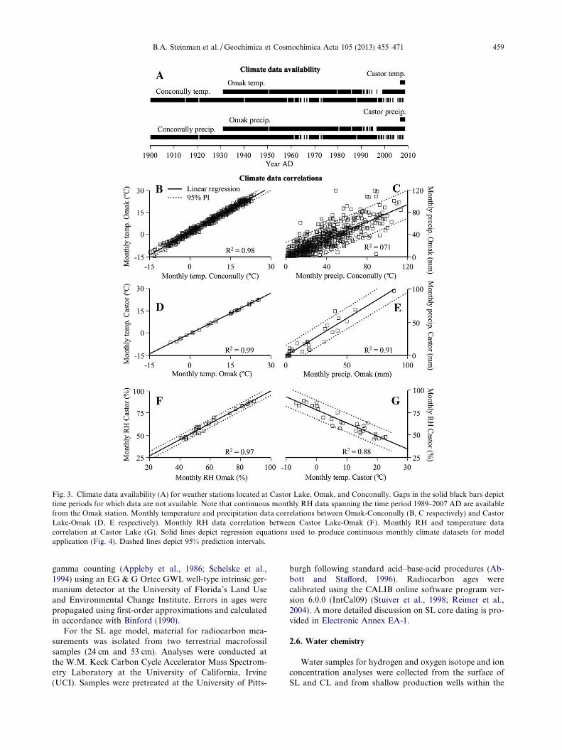
Fig. 3. Climate data availability (A) for weather stations located at Castor Lake, Omak, and Conconully. Gaps in the solid black bars depicttime periods for which data are not available. Note that continuous monthly RH data spanning the time period 1989–2007 AD are availablefrom the Omak station. Monthly temperature and precipitation data correlations between Omak-Conconully (B, C respectively) and CastorLake-Omak (D, E respectively). Monthly RH data correlation between Castor Lake-Omak (F). Monthly RH and temperature datacorrelation at Castor Lake (G). Solid lines depict regression equations used to produce continuous monthly climate datasets for modelapplication (Fig. 4). Dashed lines depict 95% prediction intervals.


gamma counting (Appleby et al., 1986; Schelske et al.,1994) using an EG & G Ortec GWL well-type intrinsic ger-manium detector at the University of Florida’s Land Useand Environmental Change Institute. Errors in ages werepropagated using first-order approximations and calculatedin accordance with Binford (1990).

For the SL age model, material for radiocarbon mea-surements was isolated from two terrestrial macrofossilsamples (24 cm and 53 cm). Analyses were conducted atthe W.M. Keck Carbon Cycle Accelerator Mass Spectrom-etry Laboratory at the University of California, Irvine(UCI). Samples were pretreated at the University of Pitts-

burgh following standard acid–base-acid procedures (Ab-bott and Stafford, 1996). Radiocarbon ages werecalibrated using the CALIB online software program ver-sion 6.0.0 (IntCal09) (Stuiver et al., 1998; Reimer et al.,2004). A more detailed discussion on SL core dating is pro-vided in Electronic Annex EA-1.

2.6. Water chemistry

Water samples for hydrogen and oxygen isotope and ionconcentration analyses were collected from the surface ofSL and CL and from shallow production wells within the

Fig. 4. Monthly average precipitation (A) temperature (B) and RH (C) for the instrumental period (1900–2007). Average November–February, March–June, and July–October values are depicted by the blue, green, and red dashed lines, respectively. Black squares (A and B)and range bars (C) depict standard deviations. Continuous precipitation (D) and temperature (E) datasets (applied in model simulations)produced using the linear regression equations depicted in Fig. 3. Uncertainty in monthly values of relative humidity (F) temperature (G) andprecipitation (H) over the instrumental period. These values represent the maximum possible range (±) of variation from the estimatedclimate variable value in the Monte Carlo simulations. (For interpretation of the references to colour in this figure legend, the reader isreferred to the web version of this article.)


lake catchments at irregular intervals between 2003 and2011. Isotope samples were collected in 30 mL polyethylenebottles by rinsing three times with sample water and thenfilling and capping the bottle underwater to remove trappedair. Ion samples were filtered through acid-cleaned 0.45 lmcellulose nitrate filters to remove suspended organic andinorganic solids. Cation samples were collected in acid-washed, 125 mL polyethylene bottles and were acidifiedwith 2 mL of ultrapure nitric acid. Anion samples were col-lected in 125 mL polyethylene bottles that were not acidwashed. All samples were stored in a cooler immediatelyafter sampling and kept refrigerated until analysis.

Isotopic ratios of lake water oxygen were measured atthe University of Arizona Environmental Isotope Labora-tory by CO2 equilibration with a Finnigan Delta S isotoperatio mass spectrometer. For hydrogen, samples were re-acted at 750 �C with Cr metal using a Finnigan H/devicecoupled to the mass spectrometer. The reported precisionis better than 0.1& for d18O and 1.0& for dD. Elementalcation concentrations were determined using InductivelyCoupled Plasma-Atomic Emission Spectrometry (ICP-AES) (Spectro Modula EOP) at the University of Pitts-

burgh. The estimated uncertainties (external reproducibil-ity) for all elements was better than ±10% of measuredvalues, based on repeated measurements of a calibrationverification standard throughout the analyses. Anion spe-cies (Cl�, F�, SO2�

4 and NO�3 ) were measured on both di-luted and undiluted samples by ion chromatography (IC)(Dionex ICS-2000) at the University of Pittsburgh. Esti-mated uncertainties on anion concentrations are lessthan ± 10% of measured values. Total alkalinityHCO�3 þ CO2�

3

� �concentrations were calculated in the field

by titration with 1.6N H2SO4 and BGMR powder indica-tors. Sulfate concentrations were directly measured usingthe IC and were inferred on the basis of molar conversionof sulfur concentrations obtained using ICP-AES.

2.7. Historical lake level estimates

Three-dimensional catchment representations for SLand CL were constructed from 1=3 arc second (�10 m reso-lution) National Elevation Data (NED) raster images, aswell as near-lake catchment survey and bathymetric data(Fig. 1). Measurements of historical lake level were ob-


tained by overlaying eleven georeferenced aerial photo-graphs and satellite images (dating between 1945 and2006) onto the lake-catchment topographic-bathymetricmaps (Fig. 2). Additional detail on the methods used toproduce the catchment maps and historical lake level esti-mates can be found in Electronic Annex EA-1.

2.8. Instrumental weather datasets

Monthly precipitation and temperature datasets span-ning the periods 1900–2007 and 1931–2007 were obtainedfrom the Conconully and Omak National Climatic DataCenter (NCDC) weather stations, respectively (Fig. 3).The datasets are largely continuous, although considerablegaps exist in both that prevent the exclusive use of either inmodel simulations. Both of these weather stations are lo-cated within 14 km and �300 m elevation of CL and SL(Fig. 1). Monthly relative humidity (RH) data collectedfrom 1989 to 2007 were obtained from the Pacific North-west Cooperative Agricultural Weather Network (AgriMet)weather station (also located in Omak). In May 2006, aCampbell Scientific weather station was installed on thenorthwestern shoreline of CL, �2 m above the lake surface.Since that time it has measured precipitation, temperature,RH, solar short wave radiation, barometric pressure andwind speed at 30 s intervals and recorded the average valueof measurements every 30 min. Precipitation amounts weremeasured using a Campbell Scientific tipping bucket withan antifreeze, snowfall adaptor installed during wintermonths. Data collected by the CL station between May2006 and October 2008 were post-processed to producemonthly values (i.e., data collected at 30 min intervals wereaveraged or, in the case of precipitation, summed).

To develop continuous century-long precipitation andtemperature datasets, the monthly Conconully and Omakweather station data were adjusted on the basis of stronglinear correlations to the monthly CL data (Fig. 3). Uncer-tainty in climate datasets was estimated on the basis of the95% prediction limits of the linear regression equationsrelating climate data from different stations (Fig. 4). Thereliance on the Conconully data to produce estimates forthe 1900–1930 time period led to a relatively large uncer-tainty range in both precipitation and temperature over this

F OF ¼ðRESSL þ RESDL � 424562 m3Þ � dt�1 RESSL þ RESDL > 424562 m3

0 RESSL þ RESDL 6 424562 m3

(ð3Þ

interval. For example, the 95% prediction limit range ofprecipitation values between Conconully and Omak is�25 mm; whereas the prediction limit range between Omakand CL is �15 mm. The sum of these two values (±40 mm/mon), was applied over the 1900–1930 period to character-ize the full range of potential uncertainty. Likewise, temper-ature values were most indeterminate over the 1900–1930period although no uncertainty was assumed thereafter

due to the very strong correlation (and correspondinglynarrow 95% prediction limit range) between temperatureat Omak and CL. Combined uncertainties (as in the1900–1930 precipitation data) were not applied to precipita-tion and temperature data in the months during the 1990swhen the Omak station did not record data. For all monthsprior to 1989, RH was calculated as a function of tempera-ture, with uncertainties determined by the 95% tempera-ture-RH prediction limit range. For all months after1989, RH values were determined using the Omak AgriMetweather station data adjusted on the basis of the linearregression with the CL station data. Electronic AnnexEA-1 contains additional detail on the methods applied toproduce the continuous weather station datasets.

2.9. Model structure

CL and SL hydrologic and isotope dynamics were simu-lated using the lake-catchment model of Steinman et al.(2010a). This model describes the hydrologic and isotopemass-balance of a lake using modified forms of the follow-ing equations:

dV L

dt¼ RI� RO ð1Þ

dðV LdLÞdt

¼ RIdI � ROdO ð2Þ

where VL is lake volume, RI and RO are the total surfaceand below ground inflows to and outflows from a lake,and d is the isotopic composition of the inflows and out-flows. The hydrologic model is defined by six separate dif-ferential equations, each corresponding to a differenttheoretical water reservoir (e.g., catchment groundwater,snowpack, shallow and deep lake volumes). Model sub-rou-tines for lake stratification, soil moisture availability, snow-pack, and surficial and subsurface inflow control volumetricfluxes to the reservoirs.

To accommodate overflow at CL (Fig. 2), which was notincluded in earlier versions of the model, a flux variable(FOF) was added to the model differential equation describ-ing the hydrologic balance of the surface lake reservoir(RESSL) (see Steinman et al., 2010a, Eq. (3)):

where RESDL (deep lake reservoir) + RESSL = total lakevolume and 424562 m3 represents the overflow volume ata depth of 13.46 m measured from the deepest part of thebasin. The complimentary differential equation describingthe oxygen isotope mass balance of RESSL was alsomodified.

Subroutines that calculate sediment d18O values on theVPDB scale were also added to the model, in order to

Fig. 5. Castor Lake (A) and Scanlon Lake (B) age-depth models. Small closed and open squares depict rejected and accepted 210Pb dates,respectively. Large open squares depict dates inferred using 137Cs. The large closed square represents a date obtained using 14C. The dashedlines represent the age models applied in this study. Horizontal bars depict the estimated age model error range. Note that the applied SL agemodel is very similar to the accepted 210Pb age model and that it passes through the 2r error range of the 14C derived age.

Fig. 6. Local meteoric water line (LMWL), local evaporation line(LEL), d18O and dD values for Castor Lake (open triangles) andScanlon Lake (open squares) surface waters, local meteoric waters(LMW) (i.e., well waters from the catchments) (open circles), andmonthly (open diamonds) and annual (cross) precipitation (esti-mated using the waterisotopes.org online calculator; Bowen andRevenaugh, 2003).


simulate the isotopic composition of endogenic andbiogenic carbonate sediments forming at CL and SL,respectively. The CL model calculates the equilibriumfractionation factor for the aragonite water system inaccordance with the equation of Kim et al. (2007):

1000 ln aAragonite-H2O ¼ 17:88ð103T�1W Þ � 31:14 ð4Þ

where aAragonite-H2O is the equilibrium fractionation factor foraragonite and water and Tw is the water temperature in de-grees Kelvin. The SL model determines the equilibriumfractionation factor for ostracod bio-calcite using the equa-tion of Kim and O’Neil (1997):

1000 ln aCalcite-H2O ¼ 18:03ð103T�1W Þ � 32:42 ð5Þ

where aCalcite-H2O is the equilibrium fractionation factor forcalcite and water. In both cases values for a are related tolake water d18O values on the Vienna Standard MeanOcean Water (VSMOW) scale in accordance with the stan-dard isotope fractionation relationship:

aCalcite=Aragonite ¼1000þ dC

1000þ dLð6Þ

where aCalcite=Aragonite is the fractionation factor of either thecalcite-water or aragonite-water systems, dC is the isotopiccomposition of either aragonite or calcite, and dL is the iso-topic composition of lake water. The model converts theo-retical aragonite and calcite d18O values from the VSMOWto the VPDB scale using the following standard equation:

dVSMOW ¼ 1:03092� dVPDB þ 30:92 ð7Þ

The SL model also applies an isotopic offset of +0.8&

(identified by von Grafenstein et al., 1999 for L. inopinata)to bio-calcite d18O values to simulate the vital isotopic effectassociated with carapace production of the Limnocytherid

ostracods. STELLA versions of the models with an accom-panying model variable and parameter table are availableas part of Electronic Annex EA-2.

2.10. Instrumental period simulations

Model simulations utilized continuous monthly temper-ature, precipitation and RH datasets spanning at least part

Table 1Castor Lake and Scanlon Lake water chemistry data.

Date Castor Lake Castor Lake Castor Lake Castor Well 2 Castor Well 1 Castor Lake Scanlon Lake Scanlon Lake Scanlon Lake Scanlon Lake5/4/06 10/1/06 7/26/07 8/20/07 8/20/07 8/21/07 5/04/06 9/30/06 7/25/07 8/21/07

Cation mg/l

Mg 242.8 450.2 487.3 80.7 44.4 499.5 473.9 2175.4 2124.3 2254.7K 34.3 60.1 57 6.8 0.8 59.4 96.8 534.7 522.9 588.6Sr 0.3 0 0.1 3.2 0.2 0.1 0.1 0.1 0.1 0.1Al 0.1 0.1 0.2 0 0.1 0.1 0.1 1 0.1 0.1Si 8.4 11.5 9.4 5.7 5.5 9.8 6.1 3.4 3.6 3.9Na 87 153.3 172.8 40.1 3.3 166.9 224.3 1184.3 1252.1 1376.6Ca 44.4 10.9 14.8 173.3 88.6 14 33.8 25.8 25 25.7Fe 0 0 0 0 0 0 0 0.1 0.1 0S No data 537.4 513.2 170.8 7.1 513.3 No data 3611.1 3271.8 3487

Anion mg/l

F 0.4 0.6 0.3 0.3 0.1 0 0 0 0 0Cl 12.9 22.7 21.3 2 0.8 36.7 34.8 161.4 135.5 136.2SO4 901.2 1594.9 1461 455.8 22.2 1522.2 2179.3 10368.3 9070.5 9706.4NO3 0 0 0 1.2 3.2 0 0 0 0 0ALK* 450 550 560 303 331 575 485 1100 1090 1130

TDS 1781.8 2854.3 2784.2 1072.1 500.2 2883.7 3534.2 15554.5 14224.2 15222.3

Cation meq/l

Mg 20 37 40.1 6.6 3.7 41.1 39 179 174.8 185.5K 0.9 1.5 1.5 0.2 0 1.5 2.5 13.7 13.4 15.1Sr 0 0 0 0.1 0 0 0 0 0 0Al 0 0 0 0 0 0 0 0.1 0 0Si 0.6 0.8 0.7 0.4 0.4 0.7 0.4 0.2 0.3 0.3Na 3.8 6.7 7.5 1.7 0.1 7.3 9.8 51.5 54.5 59.9Ca 2.2 0.5 0.7 8.6 4.4 0.7 1.7 1.3 1.2 1.3Fe 0 0 0 0 0 0 0 0 0 0

Anion meq/l

F 0 0 0 0 0 0 0 0 0 0Cl 0.4 0.6 0.6 0.1 0 1 1 4.6 3.8 3.8SO4 18.8 33.2 30.4 9.5 0.5 31.7 45.4 215.8 188.8 202.1NO3 0 0 0 0 0.1 0 0 0 0 0SO4

** No data 33.5 32 10.6 0.4 32 No data 225.2 204 217.5ALK* 9 11 11.2 6.1 6.6 11.5 9.7 22 21.8 22.6

Mg/Ca 9.1 74.0 57.3 0.8 0.8 58.7 22.9 137.7 145.7 142.7ALK/Ca 4.1 22.0 16.0 0.7 1.5 16.4 5.7 16.9 18.2 17.4Ln(ALK/Ca) 1.4 3.1 2.8 �0.3 0.4 2.8 1.7 2.8 2.9 2.9

Charge balance

Cat/An 0.98 1.04 1.2 1.13 1.21 1.16 0.95 1.01 1.14 1.15Cat/An** No data 1.03 1.15 1.05 1.21 1.15 No data 0.98 1.06 1.07

* Alkalinity measurements expressed in terms of equivalent CaCO3 (mg/l) and CO2�3 (meq/l).

** SO4 concentration inferred from S data. Cat/An** calculated using SO4 derived from S data.

B.A

.S

teinm

anet

al./G

eoch

imica

etC

osm

och

imica

Acta

105(2013)

455–471463


of the instrumental period (Fig. 4) as inputs to reconstructlake hydrologic and isotopic variations for comparison tomeasurements of lake level change and sediment core oxy-gen isotope values. To simulate climate variables for whichno long-term (i.e., multidecadal) continuous datasets exist(e.g., insolation and wind speed), monthly average valueswere applied as model inputs. In all simulations, catchmentand lake parameters such as soil available water capacitywere held constant. Each simulation (conducted on amonthly time step) lasted 128 years of which the first twentywere a model equilibration period in which averagemonthly values for all climate variables were continuouslyapplied and the remaining 108 years represented the period1900–2007.

To simulate uncertainty in the timing of carbonatemineral formation, the model was adapted to recordeither aragonite (in the case of CL) or biocalcite (in thecase of SL) theoretical d18O values at a randomly chosentime between the beginning of April and the end of Juneand to stop recording values between the beginning ofJuly and the end of August in each year of the simula-tions. The choice of April through June as the startingpoint was based on observations of whiting events madeby local residents (in the case of CL) and a generalunderstanding of ostracod life-cycles (in the case of SL,with important caveats noted in Section 3.5, below).The average of the recorded d18O values was then appliedas the carbonate mineral d18O value for that simulationyear. For both CL and SL, one-hundred model simula-tions were conducted in which climate data (Figs. 3and 4) and the timing of carbonate mineral formationwere randomized (within statistically and seasonally de-fined limits, respectively) to account for the effect ofuncertainty in these variables on simulated lake leveland sediment d18O values over the instrumental period(1900–2007). Unless otherwise noted, all modeled lakesurface elevation, depth, and d18O values discussed hereinrepresent the average of an ensemble of one-hundred dis-tinct model simulations.

3. RESULTS AND DISCUSSION

3.1. CL age model

The 210Pb age model for CL produced using the CRSmethod does not include the 137Cs peak at 1964 within a2r error range (Oldfield and Appleby, 1984) (Fig. 5). It isunlikely that 137Cs is mobile at CL, given the relativelylow organic matter content (10–20%) in the upper sequenceof the core and the well preserved laminations (see Elec-tronic Annex EA-1 for images of the CL and SL sedimentcores, age model data tables, and supplementary discussionon age model justification). The 137Cs profile was thereforeapplied instead of the ambiguous 210Pb profile to producethe upper section of the CL age model. The estimated errorrange for the time period 1900–1950 is ±10 years on the ba-sis of estimated error in the SL age model and differences inthe ages of modeled and measured variations in CL arago-nite d18O values.

3.2. SL age model

Calibration of the uppermost radiocarbon sample(24 cm) produced 5 possible ages, of which only one passedthrough the 2r error ranges of the CRS derived 210Pb dates.Therefore, to produce the SL age model, a linear functionwas applied to connect the 137Cs peak at 10.5 cm with theminimum possible age within the 2r error range of theradiocarbon sample at 24 cm (Fig. 5). This linear functionpasses through the 2r error ranges of all 210Pb measure-ments below 10.5 cm, and therefore represents the best pos-sible compromise between the 210Pb and 14C data. Anadditional linear function was applied that connects theestimated age at 24 cm with the radiocarbon date at54 cm to extend the age model through 1900. Support forthe SL age model is provided by an additional 210Pb chro-nology developed by assuming very small, non-zero unsup-ported 210Pb activities for several of the lowermost samples(Electronic Annex EA-1).

It is difficult to determine why the 210Pb measurementsof SL sediment produced a reasonable age model whenthe 210Pb data from the CL core did not, although differ-ences in coring and sediment processing methods may haveplayed a role. For example, CL 210Pb samples were ob-tained from a freeze core (rather than extruded, bagged sed-iments in the case of SL) which could have producedinaccurate bulk density measurements, on which the CRSmethod relies heavily to produce an accurate age model(Oldfield and Appleby, 1984). Differences in sediment com-position, density, and rates of deposition may also accountfor some of the discrepancy in 210Pb geochemistry betweenthe two sites.

3.3. Water chemistry measurements

CL and SL water sample isotopic values exhibited con-siderable seasonal variability (with d18O values rangingfrom �0.4 to �8.1& for CL and �13.7 to 2.7& for SL)and plot on a local evaporation line with a slope of �4.3(Fig. 6). SL waters were in almost all cases more isotopi-cally enriched than CL waters collected on the same or sim-ilar dates (Electronic Annex EA-1) indicating that SL has ahigher degree of hydrologic closure than CL. The approxi-mate water table depths in CL Well 1, CL Well 2, and theSL well were 8.5 m, 17 m, and 2.5 m below the well surface,respectively, which correspond to elevations that arehydraulically upgradient from CL and SL. Isotopic valuesof waters collected from the wells plot at the intersectionpoint of the local evaporation line (LEL) and the localmeteoric water line (LMWL) (estimated using the valuesof Bowen and Revenaugh, 2003; waterisotopes.org), rein-forcing the assertion that both lakes experience significantevaporative losses, in accordance with results from other,similar sites (Henderson and Shuman, 2009). The coherencebetween isotopic values of CL and SL catchment ground-water and theoretical meteoric values (suggested by theLMWL) indicates that no substantial isotopic enrichmentof catchment groundwater occurs as a result of surficialevaporation from soils.


In accordance with the water isotope results, ion concen-trations were higher at SL (which has summer TDS valuesof �15,000 mg/L) than at CL (which has summer TDS val-ues of �2700 mg/L) (Table 1). The proportional ion com-position of both lakes is similar as well, indicating thatCL and SL evolve along a common solute pathway thatproduces high alkalinity and Ca2+ limitation for carbonatemineral precipitation (Eugster and Jones, 1979). This maybe due in part to alkalinity generation resulting from thebacterial reduction of SO2�

4 in the water column (note thatboth CL and SL bottom water smelled strongly of H2S ineach year of the study). Water samples collected from wellsin the CL catchment have higher Ca2+ concentrations andlower alkalinity values than the lake water, further support-ing these assertions. The lack of isotopic enrichment in CLwell water combined with ion concentrations and composi-tions that are not reflective of fresh, meteoric water (i.e.,well waters contained substantial TDS concentrations) sug-gests that catchment waters likely acquire dissolved solidswhen passing through soils into the catchment aquifer.Notably, the disparity between CL well water ion concen-trations indicates a lack of spatial homogeneity in the solutecomposition of CL catchment water. A piezometer basedsampling and groundwater level monitoring programwould provide a more thorough understanding of catch-ment hydrology and groundwater composition (includingthe source of the SO2�

4 ) and could potentially provide adataset with which to validate future model predictions ofCL and SL salinity responses to climate forcing.

3.4. CL endogenic carbonate formation

At CL, aragonite precipitation from the water columnlikely occurs in the spring and early summer (April–August)as a result of physico-chemical and climatic control of thearagonite solubility product (Ksp) and Ca2+ ion concentra-tions and through biological control of dissolved inorganiccarbon (DIC) equilibria and carbonate species concentra-tions. Aragonite precipitates when the degree of saturation(X) exceeds a value of one:

X ¼ aCaaCO3

Ksp> 1 ð8Þ

where a represents the ion activity of either Ca2+ or CO2�3 .

If seed crystals are not present in solution, however, arago-nite precipitation will not occur until a critical level ofsupersaturation is reached at which the formation energyof new phase aragonite is exceeded (Koschel et al., 1983;Raidt and Koschel, 1988; Koschel, 1997).

Climate can influence aragonite formation through sea-sonal and inter-annual temperature and precipitationamount variations. Temperature influences aragonite for-mation via two interrelated mechanisms: first, by control-ling Ksp (higher temperatures result in lower Ksp values),and second, through control of primary productivity, whichtypically increases at higher temperatures resulting in re-moval of CO2 and an increase in pH (with a correspondingshift in the DIC equilibria toward the CO2�

3 species) (Keltsand Hsu, 1978). Rain/snowfall amounts can influence ara-gonite formation by controlling the delivery of Ca2+ ions

to the lake through runoff and baseflow (Shapley et al.,2005). In Ca2+ limited lakes similar to CL (Table 1), car-bonate production is limited by Ca2+ ion concentrations(Sanford and Wood, 1991) such that increased rain/snow-fall results in larger Ca2+ ion fluxes to the lake and conse-quently greater ion availability for endogenic carbonatemineral production in the water column.

The biological mechanism that relates aragonite precip-itation and primary productivity is not entirely understoodbut is thought to involve a combination of the both directand indirect influences of picoplankton. In the former case,picoplankton blooms can alter pH and induce inorganicmineral precipitation. In the latter case, they can providenucleation points that reduce the formation energy of ara-gonite crystals (Thompson et al., 1997; Hodell et al.,1998; Sondi and Juracic, 2010). At CL, biomediated arago-nite formation therefore most likely occurs in the late springafter ice breakup and the initiation of thermal stratificationof the water column. Subsequently, aragonite formsthroughout the summer months as a result of physicochem-ical effects including evaporative concentration of Ca2+ andDIC species until the Ca2+ concentration drops below thesaturation level (see Section 2.10).

XRD results indicate that aragonite is the only detect-able carbonate mineral in the CL sediment and thereforethat d18O variations in the CL core are not a result ofchanges in the carbonate mineral composition (Nelsonet al., 2011). Further, the oxygen isotopic composition ofendogenic carbonate material captured by a sediment trapdeployed in CL at a depth of �8 m from July 2005 throughMay 2006 (Nelson et al., 2011) is similar to both measuredvalues from the sediment core and theoretical estimates pre-dicted by model simulations (see Section 3.9, below), indi-cating that the proposed spring/summer aragoniteprecipitation mechanism is likely valid.

3.5. SL biogenic carbonate formation

XRD analysis of SL sediment revealed mixed carbonatemineralogy, which complicates the use of endogenic car-bonates for reconstructions of lake water oxygen isotopecomposition. Instead, ostracod carapaces, which are abun-dant in SL sediment, were used for isotopic analyses.Ostracods of the species Limnocythere staplini were identi-fied on the basis of carapace morphology (using SEM imag-ery) and studies of ostracod water chemistry tolerances(Smith, 1993; Curry, 1999; NANODe online database). Amore detailed discussion of methods used to identify thespecies living at SL (including the SEM imagery) can befound in Electronic Annex EA-1.

Ostracod molting and reproductive cycles are triggeredby changes in water temperature, food availability, and sol-ute composition and concentration. At SL, L. staplini mostlikely hatch in the spring, molt and shed their calcite carap-aces eight times until reaching adulthood in the late spring/early summer, although this cannot be confirmed withoutdirect observation of the ostracod life cycle over at least ayear. Limnocytherids form carapaces quickly, typically overseveral hours (up to 24 h in some cases), and proceedthrough growth stages to adulthood within 4–6 weeks


(Palacios-Fest et al., 2002). The short life cycle of Limnocy-

therids can potentially lead to several generations in oneyear, although the high alkalinity (>10 meq/L) and sulfate(>100 meq/L) concentrations of SL waters likely inhibitstheir growth past late summer.

All ostracod species form carapaces in isotopic disequi-librium with surrounding water, with an approximatelyconstant isotopic offset (or vital effect) from the equilibriumd18O value that is largely temperature and instar indepen-dent (see Eqs. (5)–(7), above) (von Grafenstein et al.,1999). Studies have demonstrated (De Deckker et al.,1999; Ito and Forester, 2009), however, that geochemicalvariability in ostracod carapaces can occur even in con-trolled, in vitro experiments, suggesting that this isotopicoffset likely varies (albeit by a small amount) in nature.For Lymnocythere inopinata von Grafenstein et al. (1999)determined a value of �0.8&, which we apply here to theSL ostracods, in light of the observed consistency betweenvital offsets within other families and genera.

3.6. Modeled carbonate mineral formation

The model algorithms that simulate the timing of car-bonate mineral formation at SL and CL are undoubtedlyoversimplified, as aragonite formation in the water columnand ostracod reproduction and molting cycles are largelytemperature and water chemistry dependent. By randomiz-ing this process, however, a large proportion of the uncer-tainty contributed by the timing of carbonate mineralformation is accounted for in model simulations, a muchbetter alternative than assuming constant carbonate min-eral formation over a specific time range in each year. Fu-ture efforts could focus on applying temperature or waterchemistry controls to the timing of carbonate mineralformation in the model structure, collecting additional

Fig. 7. Castor Lake (A) and Scanlon Lake (B) modeled (lines) and measuand minimum possible values of measured lake surface elevations. The gradistinct model simulations.

material using sediment traps to provide a more robustobservational dataset at CL, and directly monitoring theostracod life cycle at SL.

3.7. Comparison of measured and modeled lake surface

elevation

CL and SL lake surface elevation reconstructions basedon georeferenced aerial photographs and lake-catchmentcontour maps demonstrate considerable variability in in-ter-annual water levels (Fig. 7, Electronic Annex EA-1).At CL minimum inferred lake elevation (592.5 m) occursin 1991, with maximum lake elevation (595.5 m) duringyears of overflow in 1952, 1975, 1983 and 1998. At SL min-imum inferred lake elevation (700 m) occurs in 1973, withmaximum lake elevation (702.5 m) during 1983 and 1987.No long-term (multi-decadal) trends in lake-level changeat CL or SL are apparent between 1945 and 2006. CLand SL surface elevations of 594.25 m and 701.5 m, respec-tively, inferred using the July 2006 orthophotograph are inboth cases within 0.3 m of lake-level measurements ob-tained using Solinst Leveloggers (Steinman et al., 2010a).

Model experiments utilizing instrumental weather obser-vations from 1945 to 2007 resulted in a minimum lake sur-face elevation (�592.2 m) at CL in 1992 and maximumvalues (�595.5 m) in 1952, 1975, 1983, and 1998 (Fig. 7,Electronic Annex EA-1). The average error between in-ferred and modeled lake surface elevation at CL was�0.3 m with all but one inferred elevation (in the year1945) falling within the 2r prediction limits of model re-sults. For SL, minimum modeled lake surface elevation(�699.3 m) was reached in 1992 with the highest lake sur-face elevation (�702.5 m) occurring in 1999. The averageerror between inferred and modeled lake volume and sur-face elevation at SL was �0.5 m; however, the 1987 aerial

red (squares) water surface elevations. Error bars depict maximumy shading represents the 2r prediction intervals calculated using 100


photograph for SL is of poor quality and is the likely rea-son for the exceptionally large error measured for this year.If results from 1987 are removed, the average error de-creases to �0.4 m. In all but 4 years at SL the aerial photo-graph inferred lake surface elevations overlapped with the2r prediction limits of model simulation data.

Model estimates for lake surface elevation change from1945 to 2007 were largely consistent with observations fromaerial photographs (Fig. 7, Electronic Annex EA-1) with aslightly better correspondence at CL than at SL. The reasonsfor the discrepancy in the predictive accuracy of the CL andSL models are not entirely clear. One potential explanationlies in the conspicuous fact that, after 1980 for SL, the modelestimates for lake surface elevation are in most cases lowerthan observations. This underestimate could be related toseveral factors including inaccuracy in lake morphometrymeasurements (which would, in turn, lead to inaccuracy inthe resulting contour maps and lake level observations) orsubtle differences in precipitation, temperature, or relativehumidity at the lake, relative to the weather station-derivedvalues used within the model simulations. The latter explana-tion is more likely given that precipitation amounts, the mosthydrologically significant climate variable in the lake models,exhibits a spatial incoherence that is uncharacteristic of tem-perature and RH. The relatively low correlation of the pre-cipitation data (Fig. 3) and the correspondingly largeprediction limits suggest that precipitation amounts can varyconsiderably on monthly timescales over short distancessuch as the �14 km separating the CL and Omak weatherstations, or the�1.5 km separating CL and SL. Another pos-sible explanation lies in the fact that SL is over 100 m higherthan CL and is subject to slightly lower temperatures that re-sult in less evapotranspiration, greater snowpack amounts,and increased spring runoff, all of which lead to higher aver-age lake levels. These issues, coupled with the strong (relativeto CL) control of evaporation on SL hydrology (Steinmanet al., 2010a; Steinman and Abbott, 2012) may explain SLmodel underestimates of lake surface elevation after 1980.

3.8. The influence of precipitation amount and temperature

on lake level

Between 1900 and 1945 (i.e., prior to the period of aerialphotograph based lake level reconstruction) modeled lakelevels and volumes were on average lower than during theperiod of observation (1945–2007) (Fig. 7), an expected re-sult given that average annual precipitation amounts wereappreciably lower prior to 1945 (Fig. 4, Electronic AnnexEA-1). Model simulations predicted high lake-stands be-tween 1940 and 1950 and lake low-stands between 1920and 1940. In both cases, decadal average precipitationamounts were commensurate with the extent of the lake le-vel and volume changes. For example, in the period of pro-tracted lake low stands (1920–1940), the lowest averagedecadal precipitation amounts of the simulation period(1900–2007) occurred. Conversely, during the protractedhigh stands (1940–1950), the highest average decadal pre-cipitation amounts of the simulation period occurred. After�1975, simulated lake level varied between relative highand low points on an approximately decadal basis in

response to roughly proportionate changes in precipitationamount.

The effect of temperature on lake level and volume isnot as clear as that of precipitation. Highest average tem-peratures (and inferred increases in evaporation) occurredbetween 1980 and 1990 while the lowest lake levels oc-curred between 1930 and 1940 (Figs. 4 and 7). Similarly,average annual temperature over the period of observa-tion was higher than over the period prior to observationwhen the lowest modeled lake surface elevations oc-curred. These results support the assertions of Steinmanet al. (2010a) that CL and SL hydrologic variability ondecadal timescales is primarily controlled by variationsin precipitation amount with secondary control by tem-perature and RH.

For both lakes the relatively large uncertainty in precip-itation, temperature, and relative humidity between 1900and 1930 (Fig. 4) resulted in a comparatively large rangeof modeled depth values (Fig. 7). After �1935 the standarddeviation of depth measurements decreased substantiallyfor SL, in response to smaller climate data prediction limits.For CL the range of modeled depth values decreased andremained largely constant after 1935 except during periodsof overflow (e.g., 1952) when maximum lake level wasmaintained for longer periods of time. The relatively largestandard deviation of modeled lake depths in the early partof the 20th century illustrates the considerable hydrologicvariance imparted to lake-catchment model simulationsby uncertainties in climate data.

3.9. Comparison of measured and modeled d18O records

Measured CL sediment core d18O values vary between�6.7& (�1960) and �3.2& (�1927) over the instrumentalperiod (Fig. 8) with an average d18O value (calculated usinginterpolated data) of �4.9&. For CL, model predicted an-nual spring/summer d18O values varied between �8.6&

(2006) and �1.1& (1991) with five-year averages of the an-nual values reaching a minimum of �6.9& (1974) and amaximum of �2.8& (1992). The average modeled d18O va-lue of aragonite at CL for the entire simulation period was�5.2&, which is similar to the average value measured insediment cores. In addition, the isotopic composition ofaragonite collected using a sediment trap (Nelson et al.,2011) falls within the 2r range of model predictions, pro-viding additional support for model based estimates of lakesediment d18O values.

For SL, measured ostracod d18O values (without correc-tion for a vital offset) vary between �4.9& (�1953) and2.1& (�1926) (Fig. 8) with an average d18O value (calcu-lated using interpolated data) of �1.2&. Model predictedannual spring/summer d18O values ranged between�6.0& (1974) and 3.8& (1992) with five-year averagesreaching a minimum of �4.1& (1999) and peaking at2.5& (1992). The average modeled d18O value of biocalciteat SL for the entire simulation period was �1.2& (includ-ing the vital offset), a value that exactly matches the averagevalue measured in sediment cores. Note that an error rangeestimate has been applied to all ostracod d18O values in or-der to account for statistical variance resulting from the

Fig. 8. Modeled (gray) and measured (black) aragonite d18O values for Castor Lake (A) and Scanlon Lake (B). Thick and thin vertical graylines depict the 1r and 2r prediction intervals, respectively, of 100 distinct simulations averaged to produce the modeled values. Five yearaverages of modeled data are shown. The fine dashed lines in (B) depict the confidence interval for d18O measurements of Scanlon Lakeostracods. The closed square represents the average d18O value of sediment trap aragonite collected at CL in 2005–2006.


random sampling of �20 ostracods from each sedimentsample. A description of the methods used to produce thiserror estimate can be found in Electronic Annex EA-1.

In 77 of the 98 years of comparison, measured CL sedi-ment core d18O values are within the 2r uncertainly rangeof model predictions. For SL, a similar correspondence ex-ists, with 74 of 106 years overlapping. Effectively, thismeans that one or more model realizations exist that canreproduce the majority of measured sediment core d18Ovariations, and therefore that the model is a reasonableapproximation of the physical processes controlling lakehydrologic and isotope dynamics. Interestingly, the mostnotable time periods of inconsistency between measuredand modeled d18O values are the same for both lakes,namely, the earliest part of both records (i.e., from 1900to �1935) where model predictions are consistently lowerthan measured values, and the 1980–1990 period in whichmodel predictions for both CL and SL overestimate d18Ovalues.

The generally consistent overestimation of sedimentd18O by the model over the 1900–1935 time period canpotentially be explained by uncertainty in precipitation,which is considerably more influential than temperaturein controlling lake hydrologic and isotopic fluxes (primarilythrough changes in precipitation-evaporation balance)(Steinman and Abbott, 2012) (Figs. 4 and 8). It is possible,for example, that precipitation amounts during this timewere less than statistically derived values, and that lake lev-els were correspondingly lower and d18O values were high-er. The fact that both the CL and SL sediment cores are

more enriched in oxygen-18 during this time supports thisassertion.

Uncertainly in climate data does not, however, provide apotential explanation for the incoherence between mea-sured and modeled d18O values over the 1980–2000 timeperiod when precipitation amounts have much smaller pre-diction limits (Figs. 4 and 8). Likewise, dating uncertainties(which can explain offsets in the timing of isotopic shifts,but not the magnitude) do not provide a viable explanationgiven the smaller error range within the age models overthis interval (Fig. 5). Possible explanations are that eitherthe sediment d18O values are not reflective of water d18Ovalues during this time, or that under certain lake sedimentand water geochemical conditions (or climatic scenarios)the model fails to approximate reality. The first of thesetwo explanations is perhaps the simplest, in that a smallamount of mixing in the uppermost sediment likely oc-curred during core retrieval such that the temporal resolu-tion of the core is lower than that of in situ sediment.This could explain only part of the disparity, however, gi-ven that the average modeled (�4.7& and �0.8&, forCL and SL, respectively) and measured (�5.4& and�1.4&) sediment d18O values over the 1980–2000 intervalare considerably different. It is more likely, therefore, thatthe model predictions for this interval are incorrect. Onepossibility that is not accounted for is the incursion of airmasses from the north that are more isotopically depleted(due to transcontinental rainout) than the much more com-mon air masses from the west. This scenario would haveproduced rainfall that was more isotopically depleted along

Fig. 9. Modeled (gray) and measured (black) aragonite d18O values for Castor Lake (A) and Scanlon Lake (B) from simulations with disabledtemperature-precipitation d18O coupling. Thick and thin vertical gray lines depict the 1r and 2r prediction intervals, respectively, of 100distinct simulations averaged to produce the modeled values. Five year averages of modeled data are shown. The fine dashed lines in (B) depictthe confidence interval for d18O measurements of SL ostracods.


with correspondingly lower lake water and sediment d18Ovalues. Another possibility lies in the potential for changesin the influence of temperature on the isotopic compositionof precipitation. Several studies have shown that this as-sumed relationship (i.e., a shift of +0.6&/�C) is not neces-sarily constant through time and that it can vary spatially(Rozanski et al., 1993; Johnson and Ingram, 2004; Schmidtet al., 2007), which could explain a large proportion of thedisparity between the modeled and measured sediment d18Ovalues. To test this idea, we conducted a series of simula-tions in which the temperature-precipitation d18O controlalgorithm was disabled (i.e., turned off). Results from thesetests (Fig. 9) correlate more strongly to measured d18O val-ues over the 1980–2000 interval but do not entirely explainthe discrepancy, suggesting that either more isotopically de-pleted air masses or inaccuracy derived from some aspect ofthe lake-catchment model (or both) are the reason(s) for thedifferences.

In general, limitations in sediment core processing anddating as well as potential variation in the timing of carbon-ate mineral formation reduce the covariance between mod-eled and measured sediment core d18O values over shorter(i.e., subdecadal) time periods (Figs. 8 and 9). Further,uncertainty in climate data produces a range of possiblerealizations of modeled lake hydrologic and isotopic statesrather than just one value for each time period (i.e., manypossible depths and sediment d18O values exist for eachyear) making direct comparisons even more difficult. Thegenerally strong coherence (within age model errors),

however, between modeled and measured d18O values ondecadal timescales demonstrates that over longer time peri-ods, the model captures lake sediment isotopic variationswith reasonable accuracy. This implies that sediment oxy-gen isotope records lacking annually (or nearly annually)resolved age control, cannot be expected to strongly covarywith model isotopic predictions over the short term (i.e.,5–10 years) because of dating, climate data, and modeluncertainties, but can be expected to covary over longertime periods when comparing averaged values.

4. CONCLUSIONS

We have demonstrated that lake-catchment modelsforced with continuous, instrumental climate data are capa-ble of reproducing observed lake level changes and mea-sured sediment d18O values on decadal timescales. Thisfinding has important implications for the use of lake geo-chemical (i.e., isotope and ion) models in investigations ofmodern, future, and paleo lake responses to climate change.Of considerable importance to water management strate-gies, quantitative estimates of average, multidecadal hydro-climatic conditions spanning thousands of years couldpotentially be developed through model analyses of multi-decadal (or longer) average sediment core d18O and dD val-ues in lake systems for which modern climate andcatchment data are available as model inputs (and forwhich catchment hydrology has not significantly changed,e.g., through stream piracy). Model simulations designed


to produce such solutions would have to include stochasticas well as mean state variations in the hydroclimaticvariables and could be used to estimate, for example, pastprecipitation amounts within probabilistic limits definedby variance in the climatic variables and additional influ-ences on the lake-catchment system (e.g., catchment vegeta-tion on soil available water capacity or the effects of basininfill and morphology change through time). To success-fully conduct such a study, however, several additionalrequirements should be met such as assessment of the rela-tive influence of model initial conditions (i.e., lake hydro-logic and isotopic states prior to the initiation ofinstrumental climatic data), piezometer studies of ground-water hydrology and geochemistry, and comparison ofmodel derived, quantitative predictions of hydroclimaticvariables to direct climatological observations (e.g., weath-er station data spanning multiple decades). In the secondpaper in this series (Steinman and Abbott, 2012), we ad-dress several of these issues and explore the potential ofusing lake sediment d18O records from CL to reconstructseasonal precipitation amounts in north-centralWashington.

ACKNOWLEDGEMENTS

We thank Jeremy Moberg, Chris Helander, Broxton Bird, andJon Riedel for assistance in the field. Neil Tibert (University ofMary Washington) provided SEM images and identified ostracods.This work was funded by the US National Science FoundationAGS-PRF (AGS-1137750) and Paleo Perspectives on ClimateChange (P2C2) programs.

APPENDIX A. SUPPLEMENTARY DATA

Supplementary data associated with this article can befound, in the online version, at http://dx.doi.org/10.1016/j.gca.2012.11.026.

REFERENCES

Abbott M. B. and Stafford T. W. (1996) Radiocarbon geochemistryof ancient and modern arctic lakes. Baffin Island. Quaternary

Res. 45, 300–311.

Appleby P. G. and Oldfield F. (1978) The calculation of lead-210dates assuming a constant rate of supply of unsupported 210Pbto the sediment. Catena 5, 1–8.

Appleby P. G. and Oldfield F. (1983) The assessment of 210Pb datafrom sites with varying sediment accumulation rates. Hydrobi-

ologia 103, 29–35.

Appleby P. G., Nolan P. J., Gifford D. W., Godfrey M. J.,Oldfield F., Anderson N. J. and Battarbee R. W. (1986) 210Pbdating by low background gamma counting. Hydrobiologia 143,

21–27.

Benson L. and Paillet F. (2002) HIBAL: a hydrologic-isotopic-balance model for application to paleolake systems. Quaternary

Sci. Rev. 21, 1521–1539.

Binford M. W. (1990) Calculation and uncertainty of 210Pb datesfor PIRLA project sediment cores. J. Paleolimnol. 3, 253–267.

Bowen G. J. and Revenaugh J. (2003) Interpolating the isotopiccomposition of modern meteoric precipitation. Water Resour.

Res. 39, 1299.

Curry B. B. (1999) An environmental tolerance index for ostra-codes as indicators of physical and chemical factors in aquatichabitats. Palaeogeogr. Palaeocl. 148, 51–63.

De Deckker P., Chivas A. R. and Shelley J. M. G. (1999) Uptake ofMg and Sr in the euryhaline ostracod Cyprideis determinedfrom in vitro experiments. Palaeogeogr. Palaeocl. 148, 105–116.

Dinc�er T. (1968) The use of oxygen 18 and deuterium concentra-tions in the water balance of lakes. Water Resour. Res. 4, 1289–

1306.

Donovan J. J., Smith A. J., Panek V. A., Engstrom D. R. and ItoE. (2002) Climate-driven hydrologic transients in lake sedimentrecords: calibration of groundwater conditions using 20thCentury drought. Quat. Sci. Rev. 21, 605–624.

Eugster H. P. and Jones B. F. (1979) Behavior of major solutesduring closed-basin brine evolution. Am. J. Sci. 279, 609–631.

Gat J. R. (1970) Environmental isotope balance of Lake Tiberias.In Isotopes in hydrology. IAEA. pp. 109–127.

Gibson J. J., Prepas E. E. and McEachern P. (2002) Quantitativecomparison of lake throughflow, residency, and catchmentrunoff using stable isotopes: Modeling and results from aregional survey of Boreal lakes. J. Hydrol. 262, 128–144.

Henderson A. K. and Shuman B. N. (2009) Hydrogen and oxygenisotopic compositions of lake water in the western UnitedStates. Geol. Soc. Am. Bull. 121, 1179–1189.

Hodell D. A., Schelske C. L., Fahnenstiel G. L. and Robbins L. L.(1998) Biologically induced calcite and its isotopic compositionin Lake Ontario. Limnol. Oceanogr. 43, 187–199.

Hostetler S. and Benson L. (1990) Paleoclimatic implications of thehigh stand of Lake Lahontan derived from models of evapo-ration and lake level. Clim. Dynam. 4, 207–217.

Hostetler S. W. and Benson L. V. (1994) Stable isotopes of oxygenand hydrogen in the Truckee River-Pyramid Lake surface-water system. 2. A predictive model of d18O and d2H inPyramid Lake. Limnol. Oceanogr. 39, 356–364.

Ito E. and Forester R. M. (2009) Changes in continental ostracodeshell chemistry; uncertainty of cause. Hydrobiologia 620, 1–15.

Johnson K. R. and Ingram B. L. (2004) Spatial and temporalvariability in the stable isotope systematics of modern precip-itation in China: implications for paleoclimate reconstructions.Earth Planet. Sci. Lett. 220, 365–377.

Jones M. D., Leng M. J., Roberts N., Turkes M. and Moyeed R.(2005) A coupled calibration and modeling approach to theunderstanding of dry-land lake oxygen isotope records. J.

Paleolimnol. 34, 391–411.

Kelts K. and Hsu K. J. (1978) Freshwater carbonate sedimenta-tion. In Lakes – Chemistry, Geology, Physics (ed. A. Lerman).New York, Heidelberg, Berlin. pp. 295–323.

Kim S. and O’Neil J. R. (1997) Equilibrium and nonequilibriumoxygen isotope effects in synthetic carbonates. Geochim. Cos-

mochim. Acta 61, 3461–3475.

Kim S., O’Neil J. R., Hillaire-Marcel C. and Mucci A. (2007)Oxygen isotope fractionation between synthetic aragonite andwater: influence of temperature and Mg2+ concentration.Geochim. Cosmochim. Acta 71, 4704–4715.

Koschel R., Benndorf J., Proft G. and Recknagel F. (1983) Calciteprecipitation as a natural control mechanism of eutrophication.Arch. Hydrobiol. 98, 380–408.

Koschel R. (1997) Structure and function of pelagic calciteprecipitation in lake ecosystems. Verh. Internat. Verein. Limnol.

26, 343–349.

Nelson D. B., Abbott M. B., Steinman B. A., Polissar P. J., StansellN. D., Ortiz J. D., Rosenmeier M. F., Finney B. P. and RiedelJ. (2011) A 6000 year lake record of drought from the PacificNorthwest. P. Natl. Acad. Sci. USA 108, 3870–3875.

Oldfield F. and Appleby P. G. (1984) Empirical testing of 210Pb-dating models for lake sediments. In Lake Sediments and




Environmental History (eds. E. Y. Haworth and W. G. Lund).University of Minnesota Press, Minneapolis, Minnesota. pp.93–124.

Palacios-Fest M. R., Carreno A. L., Ortega-Ramirez J. R. andAlvarado-Valdez G. (2002) A paleoenvironmental reconstruc-tion of Laguna Babicora, Chihuahua, Mexico based onostracode paleoecology and trace element shell chemistry. J.

Paleolimnol. 27, 185–206.

Raidt H. and Koschel R. (1988) Morphology of calcite crystals inhardwater lakes. Limnologica 19, 3–12.

Reimer P. J., Baillie M. G. L., Bard E., Bayliss A., Beck J. W., BertrandC. J. H., Blackwell P. G., Buck C. E., Burr G. S., Cutler K. B., DamonP. E., Edwards R. L., Fairbanks R. G., Friedrich M., Guilderson T.P., Hogg A. G., Hughen K. A., Kromer B., McCormac F. G.,Manning S. W., Ramsey C. B., Reimer R. W., Remmele S., SouthonJ. R., Stuiver M., Talamo S., Taylor F. W., van der Plicht J. andWeyhenmeyer C. E. (2004) IntCal04 Terrestrial radiocarbon agecalibration, 26–0 ka BP. Radiocarbon 46, 1029–1058.

Rozanski K., Araguas-Araguas L. and Gonfiantini R. (1993)Isotopic patterns in modern global precipitation. In Climate

Change in Continental Isotopic Records (eds. P. K. Swart, K. L.Lohmann, J. McKenzie, S. Savin). American GeophysicalUnion, Washington, DC. pp. 1–37.

Sanford W. E. and Wood W. (1991) Brine evolution and mineraldeposition in hydrologically open evaporite basins. Am. J. Sci.

291, 687–710.

Schelske C. L., Peplow A., Brenner M. and Spencer C. N. (1994)Low-background gamma counting: applications for 210Pbdating of sediments. J. Paleolimnol. 10, 115–128.

Schmidt G. A., LeGrande A. N. and Hoffmann G. (2007) Waterisotope expressions of intrinsic and forced variability in acoupled ocean–atmosphere model. J. Geophys. Res. Atmos. 112.

http://dx.doi.org/10.1029/2006JD007781.

Shapley M. D., Ito E. and Donovan J. J. (2005) Authigenic calciumcarbonate flux in groundwater-controlled lakes: implicationsfor lacustrine paleoclimate records. Geochim. Cosmochim. Acta

69, 2517–2533.

Shapley M. D., Ito E. and Donovan J. J. (2008) Isotopic evolutionand climate paleorecords: modeling boundary effects in ground-water-dominated lakes. J. Paleolimnol. 39, 17–33.

Smith A. (1993) Lacustrine ostracodes as hydrochemical indicatorsin lakes of the north-central United States. J. Paleolimnol. 8,

121–134.

Sondi I. and Juracic M. (2010) Whiting events and the formation ofaragonite in Mediterranean karstic marine lakes: new evidenceon its biologically induced inorganic origin. Sedimentology 57,

85–95.

Steinman B. A., Rosenmeier M. F., Abbott M. B. and Bain D. J.(2010a) The isotopic and hydrologic response of small, closed-basin lakes to climate forcing from predictive models: applica-tion to paleoclimate studies in the upper Columbia River basin.Limnol. Oceanogr. 55, 2231–2245.

Steinman B. A., Rosenmeier M. F. and Abbott M. B. (2010b) Theisotopic and hydrologic response of small, closed-basin lakes toclimate forcing from predictive models: simulations of stochas-tic and mean-state precipitation variations. Limnol. Oceanogr.

55, 2246–2261.

Steinman B. A., Abbott M. B., Mann M. E., Stansell N. D. andFinney B. P. (2012) 1500 year quantitative reconstruction ofwinter precipitation in the Pacific Northwest. P. Natl. Acad.

Sci. USA 109, 11619–11623.

Steinman B. A. and Abbott M. B. (2012) Isotopic and hydrologicresponses of small, closed lakes to climate variability: Hydro-climate reconstructions from lake sediment oxygen isotoperecords and mass balance models. Geochim. Cosmochim. Acta,105, 342–359.

Stuiver M., Reimer P. J. and Braziunas T. F. (1998) High-precisionradiocarbon age calibration for terrestrial and marine samples.Radiocarbon 40, 1127–1151.

Thompson J. B., Schultze-Lam S., Beveridge T. J. and Des MaraisD. J. (1997) Whiting events: Biogenic origin due to thephotosynthetic activity of cyanobacterial picoplankton. Lim-nol. Oceanogr. 42, 133–141.

von Grafenstein U., Erlernkeuser H. and Trimborn P. (1999)Oxygen and carbon isotopes in modern fresh-water ostracodvalves: assessing vital offsets and autecological effects of interestfor paleoclimate studies. Palaeogeogr. Palaeocl. 148, 133–152.

Associate editor: Josef P. Werne

http://dx.doi.org/10.1029/2006JD007781


isotopic and hydrologic responses of small, closed lakes

Documents