issn 1725-3187 european...
TRANSCRIPT

EUROPEAN ECONOMY
Economic Papers 460 | July 2012
Fiscal Multipliers and Public Debt Dynamics in Consolidations
Jocelyn Boussard, Francisco de Castro and Matteo Salto
Economic and Financial Aff airs
ISSN 1725-3187

Economic Papers are written by the Staff of the Directorate-General for Economic and Financial Affairs, or by experts working in association with them. The Papers are intended to increase awareness of the technical work being done by staff and to seek comments and suggestions for further analysis. The views expressed are the author’s alone and do not necessarily correspond to those of the European Commission. Comments and enquiries should be addressed to: European Commission Directorate-General for Economic and Financial Affairs Publications B-1049 Brussels Belgium E-mail: [email protected] This paper exists in English only and can be downloaded from the website ec.europa.eu/economy_finance/publications A great deal of additional information is available on the Internet. It can be accessed through the Europa server (ec.europa.eu) KC-AI-12-460-EN-N ISBN 978-92-79-22981-7 doi: 10.2765/26914 © European Union, 2012

1
Fiscal Multipliers and Public Debt Dynamics in Consolidations
Jocelyn Boussard§ Francisco de Castro
† Matteo Salto
‡
European Commission European Commission European Commission
Abstract
The success of a consolidation in reducing the debt ratio depends crucially on the value of the multiplier, which
measures the impact of consolidation on growth, and on the reaction of sovereign yields to such a consolidation.
We present a theoretical framework that formalizes the response of the public debt ratio to fiscal consolidations
in relation to the value of fiscal multipliers, the starting debt level and the cyclical elasticity of the budget
balance. We also assess the role of markets confidence to fiscal consolidations under alternative scenarios. We
find that with high levels of public debt and sizeable fiscal multipliers, debt ratios are likely to increase in the
short term in response to fiscal consolidations. Hence, the typical horizon for a consolidation during crises
episodes to reduce the debt ratio is two-three years, although this horizon depends critically on the size and
persistence of fiscal multipliers and the reaction of financial markets. Anyway, such undesired debt responses
are mainly short-lived. This effect is very unlikely in non-crisis times, as it requires a number of conditions
difficult to observe at the same time, especially high fiscal multipliers.
Keywords: Fiscal consolidation; fiscal multipliers; confidence; public debt.
JEL codes: E62; H63.
§ E-mail: [email protected]
† E-mail: [email protected]
‡ E-mail: [email protected]

2
1. INTRODUCTION
EU countries have seen large debt increases since the onset of the crisis. In most EU countries debt is
now at an unprecedented level in the last fifty years. In some cases, the increases since 2007 have exceeded 20
percentage points of GDP starting from an already high level. The impact of the crisis has, for a number of
countries, compounded the dynamics of a structural deficit. The EU Member States have now started
consolidating their government finances. The increased levels of debt have led to pressure being placed on a
number of countries by the financial markets, especially in absence of sovereign bonds purchases by central
banks in secondary markets. Moreover, the recognition that insufficient attention to debt levels during "good"
economic times led to amendments of the Stability and Growth Pact (SGP), to put debt on an equal footing with
the deficit. New provisions in the SGP require EU members with a debt to GDP ratio higher than 60% to act to
put it on a downward path such that the excess of the debt ratio over this 60% value decreases by 1/20th per year
on average over three years.
A vast public debate is taking place both in the press and within the economics profession on the
effectiveness of fiscal consolidation in the current situation, centred on the question of whether "austerity can be
self-defeating". In this context, "self-defeating" would mean that "a reduction in government expenditure leads
to such a strong fall in activity that fiscal performance indicators actually get worse" This formulation stems
from Gros (2011), who refutes such a claim at the same time (for further contributions, see for example the
debate taking place on www.voxEU.org: among many Buti and Pench (2012), Cafiso and Cellini (2012), Gros
(2011), Corsetti and Müller (2012b), Cottarelli (2012) and Krugman (2012)). The debate is reflected also in the
academic literature where new research on the effects of fiscal consolidations has mushroomed.
Given the renewed relevance of the debt, both in the financial markets where financing needs are
covered and in the context of the fiscal governance in the EU, the public discussion has centred on the debt-to-
GDP ratio as the key fiscal policy indicator. The present paper aims to discuss the possibility of public debt
increases in response to fiscal consolidations and to define precisely the conditions under which such an
outcome can happen. The main result in this respect is that such a possibility is concrete, but mostly in the short
to medium term and its persistence depends on the effects on sovereign yields.
The success of a consolidation in reducing the debt ratio depends crucially on the first-year value of the
multiplier, which measures the impact of consolidation on growth, and on the reaction of sovereign yields to
such a consolidation. A cursory literature review shows that estimates or assessments of the value of the
multipliers vary enormously depending on the type of model used, the econometric technique, the economic
conditions assumed for the estimate, the conduct of monetary policy and other factors influencing the interest
rates, the composition of the adjustment and various institutional factors (from the exchange rate to credit and
labour market arrangements.)
The present paper finds a general condition that describes the impact of the adoption of consolidation
measures – compared to the situation without consolidation considered as the baseline – on the final debt ratio
as a function of starting debt ratio, cyclical budgetary semi-elasticities and fiscal multipliers. Quite intuitively
the basic condition shows that in the presence of a high starting debt ratio and a high cyclical semi-elasticity,
relatively average values of the multipliers are needed to have undesired effects of consolidations in the short
term. We also show how this conclusion changes when account is taken of the effect on yields, a particularly
relevant condition in the current sovereign crisis.
The rest of the paper is organized as follows; Section 2 discusses the factors that influence fiscal
multipliers according to theory and presents a review of the empirical literature assessing the value thereof,
jointly with existing estimates of effects of government debt and deficit on government yields. Section 3
presents the analytical framework that formalizes the debt dynamics following a consolidation shock and its
relationship with fiscal multipliers. Section 4 analyses the conditions influencing the number of years that, in
case of a short-term consolidation-induced debt-increase, are needed for a consolidation to show its effects on
the debt ratio. Finally, section 5 presents a set of conclusions and some policy implications.

3
2. LITERATURE REVIEW ON FISCAL MULTIPLIERS
The value of fiscal multipliers depends on many factors relative to the fiscal shock itself (its permanent
or temporary nature and its composition), to the economic environment (the economic situation, the economic
situation of the partner countries, the stress in the financial market or even the cyclical conditions) and to
economic policy regime (monetary and exchange rate policy). The estimated values of the fiscal multipliers are
also conditioned by the technique used to gauge them. For example, empirical estimates using Vector Auto-
Regression techniques (VAR) concern most of the times very specific fiscal shocks in terms of composition, and
always consider temporary fiscal shocks – which are not purely temporary in that fiscal variables have an
autoregressive component, while model-based evaluations like evaluations based on Dynamic Stochastic
General Equilibrium (DSGE) models can vary in this respect from purely temporary measures to fully
permanent so that comparisons are not always correct.
Given the relevance of fiscal multipliers in the discussion concerning consolidation it is however useful
to provide an overview of existing results, in particular in the two main areas of the literature which study
effects of fiscal shocks.
2.1. DSGE-BASED FISCAL MULTIPLIERS
There are different factors that affect the multipliers obtained with these models. They can be grouped
as follows: i) factors that force consumers to base consumption choices on current revenues only, such as
financial frictions; ii) factors concerning the nature of the fiscal shock, in particular the credibility of the shock
and/or its permanent or temporary nature; iii) the composition of the fiscal shock; iv) structural features of the
economy, like the presence of nominal or real rigidities; v) the type of monetary policy, and vi) the exchange
rate regime and the degree of openness of the economy. In most of these models responses to shocks are
symmetric, for which the discussion of the effects of expansionary fiscal shocks is equivalent to that of fiscal
consolidations with the reverse sign.
In general, fiscal shocks entail a negative wealth effect on households that reduces consumption and
increases labour supply, which tends to reduce real wages and consumption further. This decline in private
demand offsets most of the increased public demand, causing output to increase by less than the increase in
government consumption (see for instance Hall (2009) and Woodford (2011)). In this framework, the
consumption and investment multipliers are negative and the output spending multiplier is lower than one, even
if its value depends on the relative increase in the labour supply relative to the fall in consumption. However, the
values of the multipliers depend critically on other features of the model.
Baxter and King (1993) show that a model in which a large (permanent) stimulus causes a large wealth
effect and a large increase in labour supply can have a spending multiplier near to one as the consequent boom
in the marginal product of capital and investment compensates for the effect on consumption. However, in
general, Real Business Cycle (RBC) models in which prices are flexible and competition is perfect indicate that
the effects of fiscal policy on output pass mainly via supply effects and generate small spending multipliers,
very often below 0.5.
New Keynesian DSGE models embed frictions that affect significantly the multipliers drawn with
them. Galí et al. (2007) allow for some share of financially constrained (Rule-of-Thumb, or RoT) consumers,
which establish a closer link between current income and current consumption, thereby leading to a
consumption increase in response to a government spending rise and thus to higher multipliers.
Permanent fiscal expansions yield lower fiscal multipliers as the negative wealth effect associated to
such shocks is higher. The same mechanism holds if fiscal measures are credible. For example, QUEST
multipliers from permanent fiscal stimulus can increase from 0.3/0.4 to 0.7/0.8 if the measures taken are non-
credible or temporary (see Roeger and in't Veld (2010)).
The composition of the fiscal shock also matters. In general, short-term multipliers are found to be
higher for government expenditure shocks than for tax shocks (e.g. Coenen et al. (2012)). For instance,

4
multipliers in Roeger and in't Veld (2010) amount to 1 for government wages and government investments, to
0.5 for government purchases and to below 0.4 for transfers and taxes. Multipliers associated to government
purchases amount to 1.6 in Romer and Bernstein (2009), to 0.7 in Cogan et al. (2010). The corresponding
multiplier for temporary government expenditure shocks in QUEST is 0.8 which increases to 1.2 if monetary
policy is at the zero lower bound.1 In turn, Barrel et al. (2012) show values oscillating between 0.5 for Germany
and 1.1 for the US.
It is worth noting, however, that taxes and expenditures imply also very different long-term multipliers.
QUEST results2 show that fiscal consolidations generally involve a fundamental trade-off between short-run
pain and long-run gain. The pain arises from the negative multiplier effects of lower spending or higher taxes,
while the gain stems from the lower world interest rates and lower distortionary taxes associated with lower debt
levels. The results on both pain and gain are subject to important qualifications such as the design of a fiscal
package and the credibility thereof.
The presence of real frictions like the presence of investment adjustment costs and constraints to adapt
capacity utilisation (Burnside et al. (2004)) reduce multipliers because the presence of those frictions slows the
reaction of firms to changes in interest rates (see also (Monacelli and Perotti (2008)). According to Leeper et al.
(2011) the quantitative impact of the presence of frictions is reduced. Nominal rigidities like price or wage
rigidities have the opposite effect though (see Woodford (2011)). Price rigidities increase multipliers because
firms respond to increases in aggregate demand not by increasing prices but rather increasing output.
The role of monetary policy is one of the most important factors determining the size of government
spending multipliers. Leeper et al. (2011) show that the parameter which represents the reaction of interest rates
to expected inflation in the Taylor rule is particularly important, accounting for about 10 percent of impact
multipliers. In turn, Christiano, et al. (2011) also show that this effect is magnified in situations near to the
Keynesian liquidity trap, in which the nominal interest rate remains at the so-called "zero lower bound". In these
cases government spending multipliers amount to well above 1.
As regards the external side of the economy the degree of openness and the exchange rate regime are
key factors to explain fiscal multipliers. The fixed exchange rate regime magnifies the fiscal multiplier in
presence of capital mobility because of the monetary accommodation necessary to keep the exchange rate at
parity. Erceg and Lindé (2012a) show that spending-based consolidations in an open economy yield smaller
multipliers than tax-based ones when monetary policy is unable to adjust the exchange rate. However, the
reverse holds for small members in currency unions, or if the other members of the currency union are
consolidating and monetary policy is in a liquidity trap. Finally, a high degree of openness of the economy
reduces the multipliers as part of the effects of the fiscal shock leaks abroad via increased imports and reduced
exports (see for instance Corsetti and Mueller (2012a)).
2.2. VAR-BASED FISCAL MULTIPLIERS IN THE LITERATURE
An increasing number of empirical studies assessing the macroeconomic effects of fiscal shocks was
produced in the last decade. While the most prominent papers have focused on the U.S., there has also been a
growing body of evidence on other countries, especially European Union ones. Table 1 gathers part of the
available empirical evidence in the literature on fiscal multipliers to government expenditure shocks.
The different estimates are far from conclusive in view of the marked differences across specifications
and methodologies. For the US the literature typically finds short-term (usually 1-year) multipliers that usually
rank between 0.4 and 1, though in some studies multipliers above 1 are also obtained, while for longer horizons
the dispersion is even larger. For European countries cumulative multipliers3 over the same horizon are usually
found to be above unity. However, Burriel et al. (2010) for the euro area as a whole obtain multipliers below,
although close to unity in the short term, while after 3 years it shrinks to some 0.6. These estimates fall within
1 This range can be compared to values for government investment multipliers presented in Coenen et al. (2012) which proposes a range
of 0.9 and 1.3 or 1.1 to 2.2 depending on the model discussed. 2 This is the case for most DSGE models see for example Clinton et al. (2010). 3 The cumulative multiplier at a given period is obtained as the ratio of the cumulative response of GDP and the cumulative response of
government expenditure.

5
range of previous empirical evidence for other European countries as well as for the available evidence for the
US.
Table 1. VAR-based expenditure multipliers
[1] We define "short-term" as a time gap ranging from simultaneous effects to one year distance from the fiscal
shock.
[2] By medium-run is broadly intended a period going from 1 to 3 years after the time fiscal shock took place.
[3] Perotti (2004) distinguished four basic approaches in the literature to identify fiscal shocks in VAR: 1.
Setting a dummy variable accounting for specific episodes such as wars; 2. Imposing sign restrictions on IRFs
(pioneered in an "agnostic" way by Mountford and Uhlig (2009); 3. Exploiting Choleski ordering; 4.
Considering decision lags in policy making and fiscal variables' elasticity to economic activity (narrative).
[4] Cumulative multiplier between the 4th and 8th quarter.
[5] Impact multiplier.
[6] These two numbers are referred to expenditure multiplier respectively at the 4th and 8th quarters.
The 2012 European Commission Public Finance Report (see European Commission (2012b)) estimates
VAR models for Germany, Italy and Spain, as well as for the euro area as a whole. Except for Italy, 1-year
government spending multipliers are estimated at above 1. The same is true for the cumulative multipliers after
Studies Sample Short-term multiplier[1] Medium-term Multiplier [2] Identification strategy[3]
Blanchard and Perotti (2002) US (1947:1-1997:4) 0.5 0.5[4]
Decision lags in policy
making and imposition of
contemporaneous GDP
elasticities
US (1960:1-1979:4) 1.29 1.4
US (1980:1-2001:4) 0.36 0.28
Galí et al. (2007) US (1954:1-2003:4) 0.7 1.74 Cholesky decomposition
Ramey (2011) US (1939:1-2008:4) 0.6 to 1.2 No estimate Narrative approach
Mountford and Uhlig (2009) US (1955:1-2000:4) 0.65[5]
; 0.46; 0.28[6] -0.22
Sign restrictions on
impulse responses
Fatas and Mihov (2001) US (1960:1 - 1996:4) Similar to Galí et al. (2007) Similar to Galí et al.(2007) Cholesky decomposition
Perotti (2004) Germany (1960:1-1974:4) 0.36 0.28 Blanchard-Perotti
Germany (1975:1-1989:4)
Heppke - Falk et al. (2006) Germany (1974:1-2004:4) 0.62 1.27 Blanchard-Perotti
Baum and Koester (2011) Germany (1976:1-2009:4) 0.7 0.69Blanchard-Perotti and
Threshold VAR
Benassy-Quere and
Cimadomo (2006)Germany (1971:1-2004:4) 0.23 -0.23
FVAR and Blanchard-
Perotti
Biau and Girard (2005) France (1978:1-2003:4) 1.9 1.5 Blanchard-Perotti
Giordano et al. (2007) Italy (1982:1-2004:4) 1.2 1.7 Blanchard-Perotti
De Castro (2006) Spain (1980:1-2001:2) 1.14-1.54 0.58-1.04 Cholesky decomposition
De Castro and Hernández de
Cos (2008)Spain (1980:1-2004:4) 1.3 1 Blanchard-Perotti
De Castro and Fernández
(2011)Spain (1981:1-2008:4) 0.94 0.55 Blanchard-Perotti
IMF (2005) Portugal (1995:3-2004:4) 1.32 1.07 Blanchard-Perotti
Perotti (2004) UK (1963:1-1979:4) 0.48 0.27 Blanchard-Perotti
UK (1980:1-2001:2) -0.27 -0.6
Benassy-Quere and
Cimadomo (2006)UK (1971:1-2004:4) 0.12 -0.3
FVAR and Blanchard-
Perotti
Burriel et al. (2010) Euro Area (1981:1-2007:4) 0.87 0.85 Blanchard-Perotti
Perotti (2004) Blanchard-Perotti

6
two and three years. In the cases of Spain and the euro area as a whole, fiscal multipliers two years after the
shock seem to have increased in the most recent years.
One criticism often levied at the VAR literature, is that VAR models cannot properly account for the
fact that changes in government spending and taxes can be anticipated due to legislative and implementation
lags (Leeper, et al. (2008)) because in this case the effects of the fiscal shock would appear in the economy as
from the moment agents anticipate the government decisions. If agents are forward looking Structural VAR
(SVAR) models may fail to correctly estimate fiscal shocks, thereby leading to biased estimates of their effects
and in particular of fiscal multipliers. This is the so-called "fiscal foresight problem". The debate on this issue is
open in that if Ramey (2011) finds that fiscal foresight is a relevant issue inducing a bias on estimates of fiscal
multipliers contrary to the previous findings of Perotti (2004,) Bouakez et al. (2010) show that Ramey's results
are most likely driven by the data points relative to the Korean War episode only and should thus be not
considered of a general relevance.4
As in the case of government expenditure shocks, the bulk of the available empirical evidence on tax
multipliers refers to the United States. Results are not conclusive as even differences in the sign of multipliers
are observed. In any case, most of the empirical estimates reveal that tax shocks usually entail lower effects on
GDP than public expenditure. Table collects some of the available empirical evidence.
Table 2. VAR-based multipliers to an increase in net taxes
4 Technically, while Ramey (2011) provides evidence that SVAR-based innovations in the US as identified in Blanchard and Perotti
(2002) can be anticipated and Granger-caused by Ramey and Shapiro (1998) war episodes. However, Perotti (2004) finds little evidence that SVAR-based innovations are predictable. In turn, Bouakez et al. (2010) show that, the fiscal foresight problem is not severe enough
to preclude the use of SVAR innovations as correct measures of unanticipated fiscal shocks as Ramey's results are driven by the Korean
War episode.
Studies Sample Short-term multiplier Medium-term multiplier Identification strategy
Blanchard and Perotti (2002) US (1947:1-1997:4) Within range -0.7 and -1.3 Within range -0.4 and -1.3
Decision lags in policy
making and imposition
of contemporaneous
GDP elasticities
US (1960:1-1979:4) -1.41 -23.87
US (1980:1-2001:4) 0.7 1.55
Favero and Giavazzi (2007) US (1980:1-2006:4) 0.29 0.65 Narrative approach
Mountford and Uhlig (2009) US (1955:1-2000:4) -0.16 -2.35Sign restrictions on
impulse responses
Romer and Romer (2010) US (1945:1-2007:4) -3 Narrative approach
Germany (1960:1-1974:4) 0.29 -0.05
Germany (1975:1-1989:4) -0.04 0.59
Baum and Koester (2011) Germany (1976:1-2009:4) -0.66 -0.53Blanchard-Perotti and
TVAR
Benassy-Quere and
Cimadomo (2006)Germany (1971:1-2004:4) -1.17 -1.08
FVAR and Blanchard-
Perotti
Biau and Girard (2005) France (1978:1-2003:4) -0.5 -0.8 Blanchard-Perotti
Giordano et al. (2007) Italy (1982:1-2004:4) 0.16 Blanchard-Perotti
De Castro (2006) Spain (1980:1-2001:2) 0.05 0.39Cholesky
decomposition
Afonso and Sousa (2009) Portugal (1979:1-2007:4) + + Blanchard-Perotti
UK (1963:1-1979:4) -0.23 -0.21
UK (1980:1-2001:2) 0.43 0.7
Benassy-Quere and
Cimadomo (2006)UK (1971:1-2004:4) -0.23 -0.07
FVAR and Blanchard-
Perotti
Cloyne (2011) UK (1945-2010) Between -0.5 and -1.0 -2.5 Narrative approach
Burriel et al. (2010) Euro Area (1981-2007) -0.63 -0.49 Blanchard-Perotti
Perotti (2004) Blanchard-Perotti
Perotti (2004) Blanchard-Perotti
Perotti (2004) Blanchard-Perotti

7
The results in Blanchard and Perotti (2002) imply tax increases lead to multipliers ranging between -
0.7 and -1.3 for the first two years and somewhat lower in absolute value for the third one. For the sample
between 1980 and 2001, Perotti (2004) estimates cumulative multipliers of similar magnitude. However, Favero
and Giavazzi (2007) obtain positive (non-cumulative) multipliers to an increase of taxes for the sample 1980-
2006. The increase of output in response to a tax increase is rather counterintuitive, although this result is also
observed in other studies and for other countries (see, for instance Perotti (2004) for the cases of Germany or the
UK).
Romer and Romer (2010) employ a narrative approach for the US post-World War II period and find
very high negative tax multipliers, of almost -3% over the next three years following the shock. This contrasts
significantly with the lower multipliers calculated on the basis of tax shocks identified within VARs with the
Blanchard-Perotti methodology. Favero and Giavazzi (2010) argue that such difference is not explained by a
difference in the shocks (VAR versus narrative) but by the different models used to estimate their effects on
macro variables. They show that when the effects of shocks identified by the narrative method are analysed in
the context of a multivariate VAR (rather than using a limited information, single-equation approach),
multipliers with both methodologies turn out to be rather similar and are estimated at about unity.
As far as European countries are concerned, Blanchard and Perotti tax shocks usually lead to very low,
mostly non-significant multipliers, whereas Cloyne (2011) identifies fiscal shocks with a narrative approach à la
Romer and Romer and obtains impact multipliers to negative tax shocks between 0.5 and 1 per cent, depending
on the model specification, which rise significantly after 10-12 quarters. For the euro area as a whole, Burriel et
al. (2010) gauge net-tax multipliers between -0.6 and -0.5 for the first three years.
2.3. FISCAL MULTIPLIERS IN CRISIS PERIODS
One of the main issues discussed within the context of the "self-defeating consolidations" debate is the
non-linearity of the multipliers and specifically the fact that multipliers are expected to be larger in crisis
periods.
With DSGE models assessing the value of multipliers in crisis situations can mostly be done in an
heuristic way, by assessing the value that reasonably can be taken by the crucial parameters in crisis times as
opposed to the values that those parameters can take under normal circumstances. Among these, the factors with
highest impact on multipliers are the percentage of financially constrained agents and monetary policy being at
the so-called zero lower bound i.e. in a situation akin to the Keynesian liquidity trap. Even if DSGE models do
not make endogenous the share of consumers that are liquidity constrained, it is a reasonable assumption that
during crisis, especially crisis originated in the financial sector as the present one, the fraction of consumers that
are financially constrained increases.
Another key factor of relevance is the stance of monetary policy: the more accommodative monetary
policy, the larger the multipliers, via the impact on real interest rates. Moreover Christiano, et al. (2011) show
that multipliers are higher the larger the percentage of spending implemented under a liquidity trap, with peak
multipliers that can be larger than two while Leeper et al. (2011) find one-year spending multipliers at 1.5-1.6.
The main exceptions to linear models are constituted by Erceg and Lindé (2012b) which build a new-
Keynesian DSGE model showing that the duration of a liquidity trap is endogenous and is shorter the larger the
fiscal stimulus provided by an increase in government spending. Given that multipliers are larger the longer the
period in which the economy remains in the liquidity tap, in Erceg and Lindé the size of the multiplier is
inversely related to spending levels. The second exception is Canzoneri et al. (2012), which build on the
previous reasoning and introduce costly financial intermediation allowing financial frictions to vary counter-
cyclically. The model can thus generate impact spending multipliers which are between two and three in
recessions and 0.9 in expansions. Yearly cumulative multipliers are almost 1 and roughly two thirds
respectively. It should be noticed that these results are obtained with persistence of government shock of 0.97.

8
Recent empirical analysis tends to find that multipliers are larger in crisis periods. Auerbach and
Gorodnichenko (2010) using a regime switching structural VAR find peak values for spending multipliers of 1
and for tax multipliers of -1 in the US. When a distinction is made between expansions and recessions spending
multipliers are found respectively around 0.6 and up to 2.5, while tax multipliers become smaller but still
differentiated at -0.5 and -0.1 in recessions and expansions, respectively. Caprioli and Momigliano (2012) use a
STVAR technique on a sample of quarterly data for Italy in 1982-2011 and find multipliers that amount to 0.16
in expansions and 0.61 in recessions.
Afonso et al. (2011) use similar techniques on data from a quarterly dataset for the period 1980:4-
2009:4 for the U.S., the U.K., Germany and Italy to estimate the differences in multipliers in high financial
stress versus low financial stress regimes. They find that 3-year multipliers in high stress regimes can be twice
as large as in low stress regimes. In turn, Baum and Koester (2011) with a Threshold VAR show that public
expenditure multipliers vary depending on the size of the shock, its sign and the level of the output gap. Hence,
in low regimes or crisis periods they observe that the higher the size of the shock, the higher the spending
multiplier when government expenditure increases. Hence, a government expenditure increase of 5% may lead
to a multiplier of around 1.3, whereas when the spending increase only amounts to 2% the multiplier diminishes
to around 1. In good times though multipliers are lower and seem to behave more linearly. Finally,
Bouthevillain and Dufrenot (2011) estimate a Markov switching model on quarterly data on France for the
period 1970:1-2009:4.5 Increasing government expenditures is effective in raising GDP in recessions but not in
expansions, and similarly for a decrease in government revenues.
2.4. FISCAL MULTIPLIERS: A SUMMARY
The review of the literature presented above allows drawing the following conclusions, despite the
large variation in estimates and the difficulty in comparing them. Assessing the current size of fiscal multipliers
is complex, in that the value taken depends on its composition, its permanent nature, and on the economic
environment at large. The large majority of estimates of first-year spending multipliers in normal times are
located in the range of 0.4 to 1.2. The values are lower – quite often below 0.7 - for tax multipliers. Therefore, if
the composition of observed consolidation is taken as a guide, multipliers are expected in general to be lower
than the highest estimates: using observed changes in revenues and expenditures to GDP ratios as proxies for the
composition of the adjustment shows that in 2012 consolidation is equally shared in revenue and expenditure
measures. In the same direction also go the indications that comes from the mostly permanent nature of the
consolidation in the EU.
However, it is likely that in the current juncture impact multipliers are higher than normal because 1)
the literature stresses that in situations of crisis, and of financial crisis in particular, with many agents
constrained in the financial markets, multipliers are larger than average; and 2) monetary policy is unable or
unwilling to offset the deflationary effect of a consolidation. The specificity of the EU and of the euro area, with
high trade integration, fixed exchange rates and the necessity of consolidating at the same time and during a
period in which the rest of the world is growing well below potential add to the probability that first year fiscal
multipliers are relatively high.
The European Commission's QUEST model yields first-year output multipliers of around 0.7 and 0.4
for the Euro Area for a balanced consolidation in normal economic times, which is perceived respectively as
temporary/not credible or permanent/credible by consumers. These multipliers can become larger in a crisis
period (by a factor of one half) and even larger in a crisis period in which trade partners consolidate when they
can be multiplied roughly by a factor of 5/3.
5 True fiscal policy data at quarterly frequency are computed in France only for recent years. Data used in Bouthevillain and Dufrenot are
based on yearly time series interpolation by the OECD.

9
3. THE DEBT DYNAMICS FOLLOWING FISCAL SHOCKS
In the absence of any stock-flow adjustments,6 the government debt to GDP ratio (b) evolves according
to the following formula:7
( ) ( ) (1)
where bal represents the budget balance to GDP ratio, pbal the primary budget balance, r the average effective
interest rate on government debt and g nominal GDP growth, all in real terms. The evolution of the debt ratio
can therefore be understood as being driven by the primary balance and the snowball effect, which is the
difference between the average effective interest rate and the growth rate of the economy. Over the medium-
term, the snowball effect is of particular importance as it drives the magnitude of primary balances that are
necessary in order to ensure that government debt remains sustainable.
By definition the general government balance is the sum of a structural component and a cyclical
component. Taking ratios to GDP the balance, expressed as the sum of cyclically adjusted balance and cyclical
balance is
(2)
where is the cyclically-adjusted general government balance and is the cyclical component of the
balance. The cyclical part of the budget varies proportionally to the percentage difference of GDP to baseline,
with a coefficient equal to the semi-elasticity of budget balance .
The annual structural effort is represented by a diminution in the cyclically-adjusted primary balance,
. A permanent consolidation is thus a change in which is constant in terms of ratio of GDP, i.e.
where the notation means that the change in capb has been put in place at the first
period so that the variation of the cyclically-adjusted primary balance remains constant with respect to baseline
throughout all years onwards.
The fiscal multiplier of year i is defined as the variation of GDP over the decrease in structural
primary balance i.e. -
For the sake of notational simplicity it is also useful to define, first, the adjusted fiscal multiplier as
the percentage variation of GDP over the decrease in structural primary balance-to-GDP ratio, i.e.
-
-
Notice that corresponds to the impulse-response function used to analyse the effects of fiscal (or other)
shocks in VAR or DSGE models.
The fiscal multiplier of the growth rate, , representing the variation of growth from baseline growth
over the decrease in structural primary balance-to-GDP ratio, i.e. -
( )( - - ) with the
convention that so that the fiscal multiplier growth rate in the period in which the consolidation
6 The stock-flow adjustment is the difference between the change in government debt and the government deficit/surplus for a given
period. The main categories of stock-flow adjustments are net acquisitions of financial assets, items that do not directly affect the
Maastricht definition of debt and effects of face valuation, comprising also effects of exchange rate variation. See
http://epp.eurostat.ec.europa.eu/cache/ITY_PUBLIC/STOCK_FLOW_2011/EN/STOCK_FLOW_2011-EN.PDF 7 This formula is derived from the identity ( ) , where B represents government debt in cash terms, PBal
primary government balance and stock-flow adjustments are assumed to equal zero. The formula in the text is derived by expressing all variables as a ratio to GDP (Y)
( )
and simply rewriting
( )
and approximating
( )
with ( ) gives the
formula in the text.

10
measures are taken depends only on the first year fiscal multiplier. If the structural primary balance of the basic
scenario is small, and given that the growth rate is usually small enough, this implies that as well as in the
first period are well approximated by the fiscal multiplier as usually defined, and that in the following periods
can be approximated by the change in the multipliers.
If stock-flow adjustments are null, debt-to-GDP ratio evolves with the following dynamics:
( )
( ) (3)
Without loss of generality, assuming that the year of consolidation is year 0 and solving (3) forward
yields the debt-to-GDP ratio at the end of period n.
∏ ( - - ) - ∑ ∏ ( - - )
(4)
3.1. EXOGENOUS INTEREST RATES
It is thus possible to compute the variation of debt-to-GDP ratio in year n following a permanent
consolidation made in year 1, where as a first approximation it has been assumed that interest rates do no not
vary with consolidation.
- ∑ ∏ ( - - )
-∑ ∏ ( - - )
∑ ∑ ∏ (
- - ) (5)
Notice that since is constant and the derivative of the cyclical balance to the structural
adjustment can be computed to be
, if the baseline GDP is assumed to be close to potential GDP,
the derivative of government primary balance-to-GDP ratio with respect to the annual structural adjustment is
(6)
Substituting (6) into (5) yields the derivative of debt-to-GDP ratio at the end of year n with respect to
the annual structural adjustment.
∑ ∏ ( - - )
-∑ ( - )∏ ( - - )
-
∑ ∑ ∏ ( - - )
(7)
Let's assume that the economy was at the steady-state before the adjustment was made, meaning that
initial balance is constant, nominal growth is constant and equal to potential growth and the apparent interest
rate is constant. The marginal impact of consolidation on the debt-to-GDP ratio at the end of year n becomes:
∑ ( - )
- -∑ ( - )( - )
- - ∑ ∑ ( - )
- -
(8)
and after some algebraic manipulation:
( )
[ ( )
] ( )∑ ( ) ⏟
∑ ( ) ⏟
⏟
(9)

11
Equation (9) shows that the change in the debt-to-GDP ratio in response to a consolidation shock is the
sum of three effects: the first term is the cumulative effect of the change in growth during n years to the debt
ratio evolution; the second term is the cumulative effect of the change in balance on debt-to-GDP ratio; the third
is the cumulative effect of the consolidation. It is important to notice that (9) calculates the deviation of debt
with respect to the baseline scenario – considered here as the steady-state scenario – due to the permanent
variation in structural primary balance. It takes into account variations in growth rates, primary balance and
GDP level that the permanent consolidation – or stimulus – entails.
The short-term case corresponds to n = 1, in which case (9) becomes:
( )
- ( ( - )- ) (
( )
- ) - ( ( ) ) - (10)
Equation (10) shows that in the short-term, a consolidation affects the debt ratio both via its effect on
the primary balance and via its effect on the rate of growth of GDP. First, the debt ratio is affected by the change
in the primary balance, which, in turn affected both directly and indirectly by the consolidation measures. The
direct effect is given by the fact that consolidation measures reduce the deficit, while the indirect effect is again
given via the effect on growth; the primary balance is also affected by the growth rate of the economy via the
automatic stabilizers. The government balance is therefore given as being increased by the direct effect of
consolidation measures but reduced by the impact that these measures have on the economic growth
rate. Second, the debt ratio is increased, because if there is no significant impact of a consolidation on the
interest rate, the dynamics of the debt ratio are driven by the effect of economic growth. As consolidations
typically have a (short-term) negative impact on the economic growth rate, this leads to an increase in the debt
ratio.
Equation (10) unveils that i) a high starting level of debt leads to a large and negative impact of
consolidation on debt. The same holds for the elasticity of the government balance to the cycle; and ii) the larger
the short-term multiplier, the bigger the negative impact of consolidations on the debt ratio. Hence, from (10)
the critical multiplier can be defined as the value of the short-term fiscal multiplier beyond which a fiscal
contraction actually leads the ratio to increase on impact:
( ) (11)
where for small g can be approximated by
(12)
Table 3 shows the estimated critical multipliers for the EU27, for the 2011 levels of Maastricht debt
and using estimated cyclical semi-elasticities of government balance to the output gap to measure the reaction of
automatic stabilisers to the change in growth induced by consolidation.
Comparing the critical multipliers given in Table 3 with the results of literature referred to in Section 2
indicates that Greece is the only country where short-run debt increases could be observed even in normal times
and if consolidation is balanced. However, given the high debt levels now present in the EU and given that large
government sectors induce large cyclical semi-elasticities, around one third of the EU countries are likely to see
their debt ratio increasing compared to the baseline in the first year when a consolidation process is
implemented depending on the composition of consolidation. This is especially true if consolidation is
spending-based and is not completely credible so that figures from meta-studies are used and considering the
current crisis situation, in which case multipliers can be expected to be larger and a large part of EU countries
would be likely to be in the undesired effect area in the short term.
If one assumes that the shape of the impulse-response function follows the typical DSGE result, the
path of the adjusted multiplier can be approximated by
( ) (13)

12
with and no assumption on the sign of the long-run impulse response of GDP to fiscal
consolidation. Equation (13) allows representing the situation in which the effect of present consolidation
decreases through time. No assumption is made on the sign of the long-run multiplier: a negative value then
represents the situation in which consolidation is made via increased distortionary taxes or public investments
thus decreasing growth permanently and a negative value a situation in which hysteresis effects (see for example
de Long and Summers (2012)) are present. A positive one represents the situation in which consolidation is
made via cuts in government consumption or increases in property taxes or a situation in which interest rate are
lowered by consolidation.
Substituting (13) into (9) gives
( - )( )
- [ ( - )
- ] -
[ ( ) ( - )] [ ( - )
- - -
- -
( - ) -
-
- ] (14)
Table 3. Critical first year multipliers in EU Member States at constant interest rates in 2011
Source: Commission services' calculation
Elasticities Debt (2011)Critical
MultiplierBE 0.51 98.0 0.7BG 0.33 16.3 2.0CZ 0.36 41.2 1.3DK 0.65 46.5 0.9DE 0.54 81.2 0.7EE 0.30 6.0 2.8IE 0.44 108.2 0.7EL 0.42 165.3 0.5ES 0.43 68.5 0.9FR 0.53 85.8 0.7IT 0.49 120.1 0.6CY 0.43 71.6 0.9LV 0.30 42.6 1.4LT 0.29 38.5 1.5LU 0.44 18.2 1.6HU 0.44 80.6 0.8MT 0.38 72.0 0.9NL 0.62 65.2 0.8AT 0.47 72.2 0.8PL 0.38 56.3 1.1PT 0.45 107.8 0.7RO 0.32 33.3 1.5SI 0.45 47.6 1.1SK 0.33 43.3 1.3FI 0.58 48.6 0.9SE 0.61 38.4 1.0UK 0.46 85.7 0.8

13
3.2. ENDOGENOUS INTEREST RATES
It is often argued that consolidation or stimulus measures have an impact on yields, influencing the
future path of debt. Indeed, if we assume that apparent interest rates paid on the stock of debt vary with the
implementation of a variation of the structural primary balance the overall variation of the debt-to-GDP ratio at
the end of period n becomes:
( )∑
∑ ( ) ∑
⏟
(15)
where
is the variation of the apparent interest rate at period i and
is the debt-to-GDP variation
calculated in the previous section with constant interest rates. A negative
indicates that consolidation effort
improve market's confidence in government bonds and reduce yields. To describe the variation of yields, as a
function of debt, deficit, market expectations and market short-termism is expressed as
. Yields vary by
assuming that they depend on the expected solvability of the government given the level of rates. Yields depend
on the expected level of debt at a certain horizon h assuming baseline rates: a small h means that financial
markets are short-sighted and high h means that financial long-sighted. Assuming adaptive expectations in a
sense that agents revise them if the actual level of debt differs from what was expected, we thus have:
(16)
where stands for the yield sensitivity to structural primary balance, growth perspective and other external
factors that affect confidence and fort the yield sensitivity to the debt level.8
The variation of the debt-to-GDP ratio at the end of the period n then becomes
( ) ∑
∑( ) ∑
⏟
( )
[( ) ( ) ( )
( )
]
⏟
( ) ∑
∑( ) ∑
⏟
(17)
The predictions of economic theory on the effects of fiscal policy variables on interest rates are not
univocal. The traditional Keynesian analysis well represented by the IS/LM model stresses the role of deficit: an
increase in deficit tends to increase government yields and consequently interest rates via demand pressure. A
similar argument holds for New Keynesian DSGE models, that incorporate a Taylor rule by which interest rates
react positively to future inflation generated by the increased demand due to a deficit increase or a
devaluation/depreciation of the currency. These models however refer to short-term interest rates, while the
relevant rate for the economy is probably the long-term interest rate, which better reflects marginal productivity
of capital.
8 It is to be remarked the assumption that financial markets are assumed not to take into account the consequences of their own behaviour
on debt evolution. This seems coherent with the assumption of myopic behaviour.

14
Table 4. Fiscal consolidation and the cost of debt
Source: Commission services' calculation
Table 4 provides a summary of the literature documenting the effects of fiscal variables on interest
rates. Despite some dispersion in the estimates, higher fiscal deficits and public debt ratios seem to lead to
higher interest rates too. On average, the available evidence suggest that increases in public deficits and debt
ratios of around 1% of GDP may entail long-term interest rate rises of around 50 basis points and about 5 basis
points, respectively. Both estimates are compatible as a permanent increase in deficits by one point of GDP
Studies SampleShort term int. rates
(5 years)
Long term int. rates
(10 years)Approach
Engen and Hubbard (2004) US (1976-2003) Debt 0.28 Debt 0.30 Vector auto regression (VAR)
Gale and Orszag (2004) US (1956-2000) Deficit 0.3/0.7 LS and ML estimates
Eaton and Fernandez (1995) Survey of literature
Increased debt levels raise the
probability of default. Higher
public debt increases risk premia
Literature review
Manasse, Roubini and
Schimmelpfenning (2003)
47 economies with market
access (1970-2002)
Increased debt levels raise the
probability of default. Higher
public debt increases risk premia
Logit and binary recursive
tree analysis
Laubach (2010) US (1976:1-2006:2)
Deficit : 0.23
Debt : 0.032
for the 5-year-ahead 5-year
forward rate
Deficit : 0.20-0.29;
Debt : 0.022-0.044
for the 5-year-ahead 10-year
forward rate
LS and IV regression
Thomas and Wu (2009) US (1983-2005) Deficit : 0.48-0.60 Deficit : 0.30-0.46 LS regression
Dai and Philippon (2005) US (1970:1-2003:3) Deficit : 0.4-0.5
VAR that incorporates a no-
arbitrage affine term-structure
model with a set of structural
restrictions to identify fiscal
policy shocks
Ardagna et al. (2004)16 OECD countries (1960-
2002); (1975-2002)
1% of GDP increase in primary
deficit:
+10 bp (static specification)
+150 bp (P-VAR)
Non-linear effects of public debt
Panel and
Panel VAR
Ardagna (2009)16 OECD countries (1960-
2002) yearly data
Deficit : 0.24-0.42
Debt: 0.04-0.06
interest rate increases by 162
basis points in periods of
worsening primary government
balance and decreases by 124
basis points on average in
consolidation periods
Panel
Faini (2006) 10 EA members (1979-2002) Debt: 0.53 Panel
Codogno et al. (2003)9 EMU founding members
(1999-2002)
Debt: Lowest in Netherlands
0.05; highest in Portugal 0.08
Debt ratio of 50 points higher
than Germany: +47.5 b.p.
Time series inspection and
SURE estimates
Bernoth et al. (2004)13 EMU countries (1999-
2002)
Debt ratio of 25 points higher
than Germany: +30 b.p.; Panel
Barrios et al. (2009)7 Euro area countries (2003-
2009)
Government surplus: -0.024 Debt
: 0.003LS and IV regression
Schucknecht et al. (2010) 12 countries (1991-2002)
+marginal debt (benchmark
country): 0.09 b.p. before 2008;
1.18 b.p. after.
Panel
European Commission
(2010)
10 founding members (1999-
2009)Debt: 12-18 basis points Panel
Iara and Wolf (2010) 11 EA countries (1999-2009) Debt: 0.93-1.40 Panel (GMM)

15
would increase the debt to GDP ratio by the same amount and have thus a cumulative effect in interest rates of
the same order of magnitude. However, these effects may be non-linear. The effects on government yields are
expected to rise with the stock of public debt, mainly via the risk premium linked with sustainability concerns.
Accordingly, insofar as fiscal consolidations succeeded in reducing public debt, their associated short-term pain
would be lower the larger the initial stock of public debt.
4. THE RESPONSES OF PUBLIC DEBT TO FISCAL CONSOLIDATIONS
The comparison between the critical multipliers and the available empirical evidence of fiscal
multipliers in the literature shows that it is not impossible that in the current situation consolidation leads to
higher debt in the short run. This Section looks at how the multipliers affect the debt dynamics following a
consolidation, before the next Section introduces possible effects of consolidations on interest rates and moves
to look at debt dynamics from a more medium-term point of view.
As shown in equation (9) the evolution of the debt ratio, in the absence of any effect on government
yields, it is the sum of same three effects: i) the cumulative effect of growth on debt, this effect being larger the
larger initial debt stock and the higher the multipliers; ii) The cumulative effect of growth on government
balance, which increases with the size of the multipliers and the size of automatic stabilisers, and; iii) the
cumulative effect from the adjustment of government balance, with this effect being inversely related to the
number of years and the size of the consolidation implemented.
The first two effects are act to increase the debt ratio, while the third acts to decrease it. One way to
look at the medium-term effects of a consolidation, then, is to consider the number of years n* (hereafter "the
critical year")9 necessary for the consolidation to lead to a decrease in debt with respect to a baseline scenario. In
terms of equation (9) this is equivalent to the number of years necessary to bring
to zero (or be negative).
Figure 1. Critical year and underlying debt trend
Source: Commission services.
9 Notice that n*represents the number of years starting from the year of consolidation. If consolidation is implemented in year 1, n*
represents the critical year. Therefore n*=1 means that there is no debt increase at all, while n*=2 indicates that the debt increase lasts
one year and so on.
92%
94%
96%
98%
100%
102%
104%
0 1 2 3 4 5 6 7 8
year
baseline scenario deviation
94%
96%
98%
100%
102%
104%
106%
108%
110%
112%
0 1 2 3 4 5 6 7 8
year
baseline scenario deviation
16
The critical period n* is different from the number of years required for the debt to go below its starting
value in year 0 unless the baseline is the steady state of constant debt ratio. Figure 1 shows illustrative paths for
the debt under baseline and consolidation scenarios, for a constant baseline in the left-hand panel and an
increasing one in the right-hand panel. It shows that, while in the case of a stable baseline scenario n* coincides
with the year in which the debt level returns to its level in the consolidation year, this does not happen when the
baseline scenario is increasing and the solid line representing the path of debt-to-GDP ratio following a
consolidation returns to the starting level only after crossing the dotted line representing the baseline scenario (if
ever). When looking at the effects of a consolidation on the debt, the relevant comparison depends on the aim of
the exercise. The debt trajectory under a consolidation should be compared to the baseline debt if we are purely
interested in the effect of the consolidation per se; however, if there is an overall question of debt sustainability
the debt after a consolidation will also need to be compared to the actual starting level of debt.
In order to model debt dynamics and calculate the value of the critical year n* under different
consolidation scenarios, to run debt simulations under different consolidation scenarios, a clear picture of the
reaction of GDP to consolidation in future years ( ) is necessary, bearing in mind that is likely to change over
time. The higher the multipliers in the first year and the longer the change in GDP induced by the consolidation,
the larger the value of n* and the longer it will take for a consolidation to be effective.
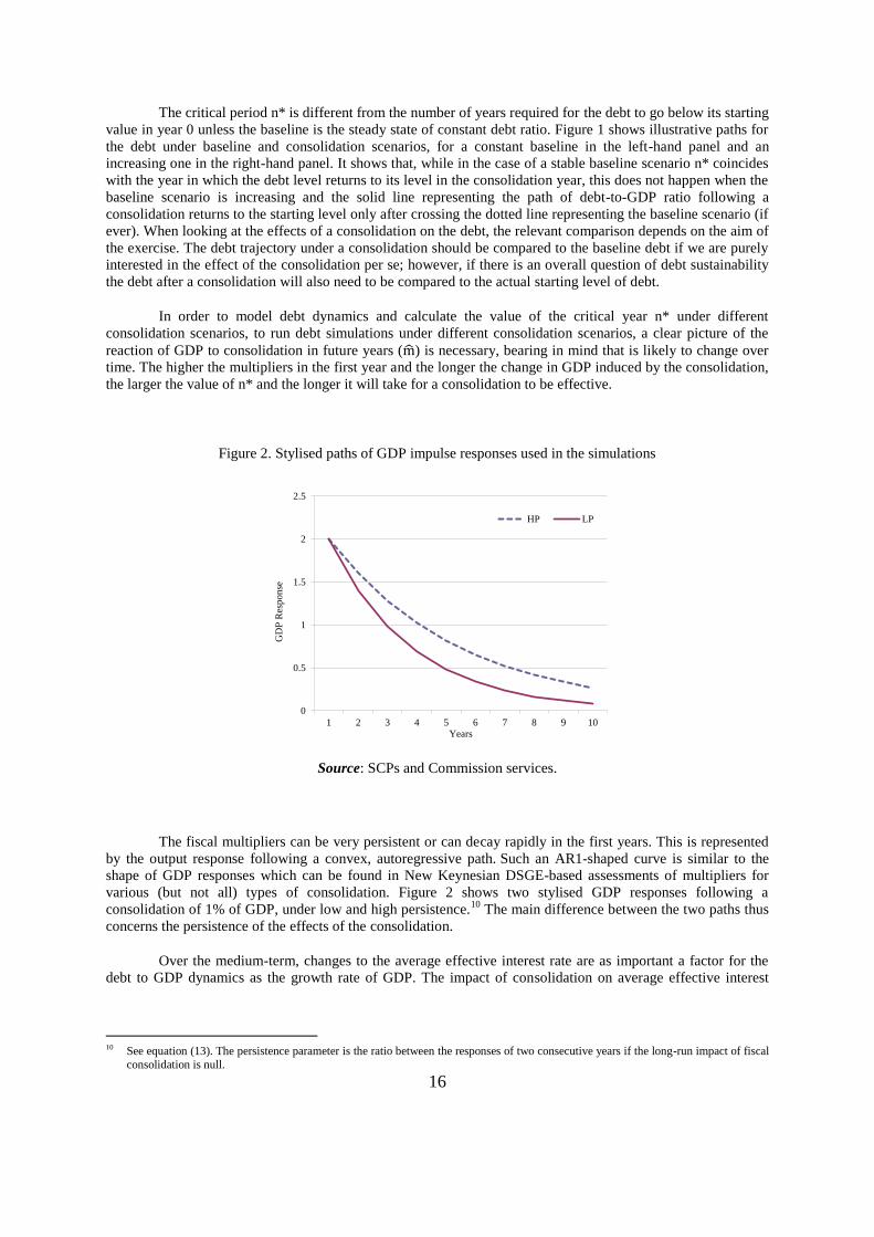
Figure 2. Stylised paths of GDP impulse responses used in the simulations
Source: SCPs and Commission services.
The fiscal multipliers can be very persistent or can decay rapidly in the first years. This is represented
by the output response following a convex, autoregressive path. Such an AR1-shaped curve is similar to the
shape of GDP responses which can be found in New Keynesian DSGE-based assessments of multipliers for
various (but not all) types of consolidation. Figure 2 shows two stylised GDP responses following a
consolidation of 1% of GDP, under low and high persistence.10
The main difference between the two paths thus
concerns the persistence of the effects of the consolidation.
Over the medium-term, changes to the average effective interest rate are as important a factor for the
debt to GDP dynamics as the growth rate of GDP. The impact of consolidation on average effective interest
10 See equation (13). The persistence parameter is the ratio between the responses of two consecutive years if the long-run impact of fiscal
consolidation is null.
0
0.5
1
1.5
2
2.5
1 2 3 4 5 6 7 8 9 10
GD
P R
esp
onse
Years
HP LP

17
rates is more visible in the medium-term than in the short-term, with limited first-year impact on the debt
level.11
As shown in equation (17), taking into account the effects of changes in apparent interest rates adds a
fourth element to the drivers of debt dynamics that affects n* critically. The interest rate effect consists of the
increased (or decreased if the interest rate diminishes) future debt burden related to the increased interest
payments on the rollover of existing debt stock, and, second, the increased payments on the new debt related to
future deficits.
The sign of this effect however is not clear cut as it depends crucially on the way market expectations
are generated.12
The normal case, in line with the results of the literature presented in Section 3, is the case in
which a consolidation improves the market's confidence in government bonds and reduces yields so that a
consolidation leads to a lower average effective interest rate r. In this case, the effect of a consolidation on debt
is reinforced and debt-to-GDP ratios are likely to decrease at a higher speed (or increase less) than with constant
yields. If, on the contrary, the market reacts to consolidation by increasing yields and consequently average
effective interest rates, the effect of this term is the opposite. Such an effect would be unusual, but by no means
just a theoretical possibility.
In the simulations ahead it is assumed that the change on average effective interest rates is driven by
the risk premium so that the change of the average effective interest rate due to a consolidation a is expressed
as
The parameter h, de horizon of financial markets, plays a key role. In particular h=1 indicates that
markets look at the debt in the year of the consolidation, which implies a high degree of myopia of financial
markets.13
In this context, a high sensitivity of interest rates to the debt ratio could actually lead to increases in
public debt levels. This could happen if a consolidation increases the debt ratio due to the denominator effect,
which then leads to increase in interest rates which then further increase the debt ratio and so on. A positive
means that the decrease in the risk premium due to the decrease in structural deficit does not offset the increase
in central bank's real rates due to deflationary pressures.
The way
is expressed allows for the impact of quantitative effects of consolidation on interest rates
to be easily factored into the analysis. Such effects can be very relevant in crisis situations and are not well
modelled in linear models. The formula does, however, have the disadvantage that it does not take into account
the spreading of the changes of government yields on the rest of the economy – or de facto it assumes that such
effects are relatively small – because the path of the multiplier is independent from the reaction of interest
rates.14
Moreover, the linear form of the interest rate function prevents from taking into account thresholds
effects, another characteristic which the literature shows being potentially relevant in crisis periods.
11 A more immediate impact can be seen on the yield of government debt, which may react more abruptly as borrowing goes up or down.
The more muted effect on the interest rate is partly driven by the fact that only a share of overall debt needs to be reissued in any one
year and so the effect on the average (or apparent) interest rate is more modest. An increase in interest rate of 50 basis points has a
modest impact in the first year if 20% of the debt is rolled over every year: for example with debt ratio at 100% and a 20% rollover, 50 basis points increase means an additional 0.1% increase in deficit/debt. Nevertheless, in difficult times, there have been sizeable
increases in the apparent interest rate that can be observed in the data. For example, between 1974 and 1975 the apparent interest rate
increased from 15.7 to 22.2 in Denmark, while it increased from 8.3 to 15.2 in Portugal between 1980 and 1981. Conversely to these large sharp increases, decreases are often more gradual even when sustained, as was the case for the countries with higher yields at the
entry in the EMU. 12 Of course, other variables such as the conduct of monetary policy also affect this term. 13 It is to be remarked the assumption that financial markets are assumed not to take into account the consequences of their own behaviour
on debt evolution. This is a simplifying assumption which has very reduced practical impact if myopia is interpreted as backward-
looking behaviour or if the horizon in question is as short as one or two years. Notice that the formula could apply to new emissions as well, without substantive
14 Notice that if interest rates decrease with consolidation, the formula for the change in r reinforces the possibility of undesired effects. In
DSGE models multipliers decrease with interest rates.

18
4.1. THE DISTRIBUTION OF n*
To study the impact of each parameter of the equation on the value of n*, we simulate a randomly
distributed vector ( ) respectively initial level of debt, impact multiplier, response
of interest rates to changes in short-term growth and fiscal outlook, persistence of the multiplier, long-run
multiplier, sensitivity of interest rates to government debt, baseline nominal growth, baseline nominal rate,
baseline primary balance and semi-elasticity of budget balance to GDP. Each parameter follow a normal
distribution except for that follows a gamma distribution to better account for the fact that it is assumed
always positive and with a higher probability of high values than with a normal distribution ("fat tail" effect).
Table 5 below summarizes the distribution of each parameter during a crisis episode:
We calculate the value of n* for each combination of these parameters and different values of the
market horizon h, and given the size of their confidence interval we estimate their marginal impact on the value
of n* in a linear equation, summarized in Table 6:
Table 5. Distribution of parameters affecting n*
b0 m µ g r pbal
min 0.16 -1.14 -0.53 0.36 -0.36 0.00 -0.05 -0.06 -0.05 0.30
max 1.82 2.78 0.74 0.94 0.34 0.44 0.10 0.09 0.03 0.68
median 1.00 1.00 0.00 0.65 0.00 0.03 0.02 0.02 -0.01 0.50
std 0.20 0.50 0.15 0.08 0.10 0.04 0.02 0.02 0.01 0.05
95% confidence
interval
[0.61;
1.40]
[0.02;
1.98]
[-0.3;
0.29]
[0.5;
0.8]
[-0.2;
0.2]
[0;
0.13]
[-0.02;
0.06]
[-0.02;
0.06]
[-0.03;
0.01]
[0.4;
0.6]
Table 6. n* and markets horizon
b0 m µ g r pbal
confidence
interval size
0.79 1.96 0.59 0.3 0.39 0.13 0.08 0.08 0.04 0.2
impact on nstar
h = 1
1.0 3.1 1.1 0.5 0.1 0.7 -0.3 0.0 -0.1 0.4
impact on nstar
h = 2
0.7 2.9 0.9 0.5 0.1 0.1 -0.1 0.0 -0.1 0.3
impact on nstar
h = 3
0.6 2.6 0.9 0.4 0.1 -0.2 -0.1 0.0 0.0 0.3
The parameters having the biggest impact on n* are, in descending order of impact : the impact
multiplier, the response of interest rate to consolidation, the initial level of debt, the sensitivity of rates to
expected debt, the multiplier persistence, the semi-elasticity of budget balance, the baseline nominal growth and
the long-run multiplier. The baseline nominal rate and primary balance have almost no impact on n*.
The relevance of the parameter that measures the reaction of interest rates to debt - γ - highly depends
on the short-termism of the markets: with short-sighted markets (low h) the higher the sensitivity of rates to
solvability, the less effective is consolidation in bringing down the debt ratio under the case in which multipliers

19
are above the critical value. On the contrary with more rational markets the higher is the sensitivity to solvability
the more efficient is consolidation. The non-significance of baseline interest rate depends on the fact that
changes induced by consolidation are large and affect n* and it should not be interpreted as a claim that
sovereign yields are irrelevant.
The value of the baseline scenario does not substantially affect the critical year: n* increases only
modestly with baseline growth, average effective rates and output gap, and decreases moderately with the
baseline primary balance. On the other hand, the multipliers are relevant. Impact multipliers have a significant
impact on debt dynamics since an increase in multipliers by one point leads to a 6 quarters increase in n*. The
long-term multiplier and the semi-elasticity of budget balance have a similar impact on n*.15
Finally, a general picture of the previous results shows that for any given debt-to-GDP ratio, the value
of n* increases with the impact multiplier when consolidation has no effect on yields. A three year horizon is
reached only with very high debt (140% of GDP) and multiplier at around 1.4.
In what follows we will try to characterize the conditional distribution of n*, the probability that debt
diverges following a consolidation and the size of the peak in debt in the cases where it does not diverge.
Indeed, as we have seen, in most cases, if the impact multiplier is higher than the critical multiplier, debt
increases on impact and slowly decreases as GDP returns to its long-run level and primary balance is higher.
In the basic case where all parameters are independent, which seems unlikely but provides a good
ground for comparison, the distribution of n* is described in Figure 3 and Table 7. The simulations yield a close
to 1 probability that consolidation becomes efficient in less than four years, with almost surely no divergence.
Debt always goes back below the baseline level in less than 4 years in most cases (ten years markets' myopia is
high), with a peak at two years: in fifty percents of the cases, debt increases on impact with respect to the
baseline but falls below baseline the year after the consolidation started. Moreover, with relatively low values of
gamma and linearity between debt and rate, it is almost impossible to generate cases of divergence, and the
value of n* does not depend on markets' degree of myopia.
Figure 3. Stylised paths of GDP impulse responses used in the simulations
15 Given these result in what follows it is assumed to set real growth, apparent rate, primary balance, output gap and long-term multiplier
at zero and the budgetary semi-elasticity at 0.5. Multiplier persistence is fixed at 0.7.
0%
5%
10%
15%
20%
25%
30%
35%
40%
45%
1 2 3 4 5 6 7 8 9 10
h=1
h=2
h=3

20
Table 7. Distribution function of n* for different markets horizon
h=1 h=2 h=3
P(n*<=4) 98.74% 99.19% 99.33%
P(n*>4) 1.26% 0.81% 0.67%
P(n*>10) 0.04% 0.00% 0.00%
P(n*=inf) 0.00% 0.00% 0.00%
Finally Figure 4 shows the distribution of the size of the peak – which is the maximum increase of debt
relative to the baseline – among cases where debt increases on impact but does not diverge. The maximum
increase in those cases is of four percentage points and the distribution is similar to the distribution of n*. For
the different values of h, the correlations between n* and the size of the peak is comprised between 0.78 and
0.81, which confirms the fact that the impact parameters are the most important parameters, the persistence and
dynamics of rates accounting for about 20% of the variation of n*.
Figure 4. Distribution of the size of the peak of increase in the debt ratio
Nevertheless it seems unlikely that the parameters are independent. Indeed there are some arguments in
favour of specific correlations. For instance, it can be argued that agents are more Ricardian when government
debt is high, thus leading to a smaller impact multiplier when debt is high (negative correlation between m and
b0). Also, markets may be more concerned about the overall sustainability of public finance when debt is high,
and thus be more inclined to welcome a reduction of the primary deficit (negative correlation between and b0)
and more sensitive to variations of debt (positive correlation between and b0). Also, a deeper analysis of
economic mechanisms gives two arguments in favour of a high positive correlation between impact multipliers
0 0.005 0.01 0.015 0.02 0.025 0.03 0.035 0.040
200
400
600
800
1000
1200
1400
1600
1800
2000
Blue : h = 1
Green : h=2
Red : h=3

21
and the response of interest rates. Firstly the IS-LM model suggests for instance that the impact on GDP of
changes in government balance highly depends on the reaction of interest rates, highly linked to the interest rate
on public debt: if rates decrease with consolidation the multiplier is likely to be low. Secondly if the multiplier is
high, markets that are sensitive to short-term growth may increase the risk-premium on government bonds.
To determine the distribution of n* one needs to make assumption on the values of these correlations.
We focused our attention one four specific pairwise correlations: the initial level of debt with the impact
multiplier, with the response of interest rates and with the sensitivity of rates to expect debt, as well as the
correlation between the impact multiplier and the response of interest rates. We first draw the results with the
following correlations:
Table 8. Parameters correlations
-0.5
-0.5
0.7
0.9
The distributions of n* stemming from the correlations in Table 8 are shown in Figure 5, while the
corresponding distribution function is summarized in Table 9. Divergence is here possible in 0.09% of the cases
when the degree of markets' myopia is high, and the distribution of n* is slightly moved to the left with more
than double the probability that n* is higher than 4. The distribution of the size of the peak resembles the basic
case's one with higher maximum values of the peak (around seven percentage points), and the correlation
between n* and the size of the peak remains high (comprised between 0.5 and 0.8)
Figure 5. Distribution function of n* from correlations in Table 8
0%
5%
10%
15%
20%
25%
30%
35%
40%
45%
1 2 3 4 5 6 7 8 9 10
h=1
h=2
h=3

22
Table 9. Distribution function of n* from correlations in Table 8
h=1 h=2 h=3
P(n*<=4) 97.06% 97.80% 98.40%
P(n*>4) 2.94% 2.20% 1.60%
P(n*>10) 0.21% 0.11% 0.04%
P(n*=inf) 0.09% 0.00% 0.00%
Figure 6. Distribution of the size of the peak of increase in the debt ratio from correlations in Table 8
4.2. DEBT RESPONSES AND n* UNDER SPECIFIC CONFIGURATIONS
The left panel of Figure 7 shows the debt-to-GDP ratio dynamics for the low-persistence multipliers
path under different assumptions about the impact multiplier. The baseline scenario is one of a constant debt
ratio of 100% of GDP. The Graph shows debt dynamics for a persistence rate of 0.5,16
with first year multipliers
of 0.5, 1 and 1.5. All values for the first-year multiplier that lie below the 0.7 level will correspond to an
improved debt ratio from the first year – this is so by construction as the 0.7 level corresponds to the critical
value for the multiplier. It should be noted that a first year multiplier of 1.5 is on the high side of existing
estimates as it is the estimate of a temporary consolidation based on government spending.
The right panel of Figure 7 shows the case for a high persistence parameter (0.8) of the GDP
response. The higher persistence of the effects of consolidation generates longer-lasting negative effects from
fiscal consolidation. If the first-year multiplier is 1.5 the consolidation-based debt increase lasts for one more
year so that three years are needed – taking into account the fact that year 1 is the year in which the
consolidation is implemented – before debt goes below baseline.
16 0.6/0.7 is the ratio of second to first year GDP responses in the case of composition-balanced permanent consolidation in European
Commission (2010a). This is the basis for the choice of 0.5 as low persistence and 0.8 as high persistence parameters. Note that the
persistence in the following years is however smaller. Values of the GDP responses broadly constant for the first three years are very commonly found in VAR estimates. This wold make raise an hump-shaped GDP response with the consequence that the debt increases
following a consolidation would be reversed only after three years for values of the impact multiplier of 1.5. This being the only
difference, the case is not developed here.
0 0.01 0.02 0.03 0.04 0.05 0.06 0.070
500
1000
1500
2000
2500
3000
3500
Blue : h = 1
Green : h=2
Red : h=3

23
Figure 7. Debt dynamics (baseline steady state, b0 = 100%), no effect on interest rates
Figure 8 show the effects for the two cases of low and high persistence of changes in the interest rate
on the critical number of years n* under the condition that the first-year multiplier is 1.5. It can be seen that the
critical number of years before the debt is reduced to below its starting level in absence of effects on the interest
rates remains the same as shown in Figure 7, for the case without interest rates, for changes in the interest rates
which are in line with empirical evidence. In the simulation, if market confidence reacts positively to a
consolidation the number of years needed to bring debt levels back to original values reduces, especially in the
case of high persistence of multipliers. Again, the persistence of the multiplier affects critically the number of
years needed for the debt ratio to resume to initial values prior to the fiscal consolidation.
The size of the consolidation effort does not affect n* though. A higher fiscal effort entails a higher
initial increase of the debt ratio. However, such a higher fiscal effort also implies that the pace of debt reduction
after the initial rise is also quicker, thereby leaving the value of n* unchanged.
Figure 8. Debt dynamics (baseline steady state, b0 = 100% and m=1.5) with effects on interest rates
93%
94%
95%
96%
97%
98%
99%
100%
101%
102%
0 1 2 3 4 5 6year
m = 0.5
m = 1
m = 1,5
baseline
High persistence
93%
94%
95%
96%
97%
98%
99%
100%
101%
102%
0 1 2 3 4 5 6year
m = 0.5
m = 1
m = 1,5
baseline
Low persistence
90%
92%
94%
96%
98%
100%
102%
0 1 2 3 4 5 6
year
µ = 0 µ = -0.3 baseline
90%
92%
94%
96%
98%
100%
102%
0 1 2 3 4 5 6
year
µ = 0 µ = -0.3 baseline
High persistenceLow persistence

24
4.3. FINANCIAL MARKETS MYOPIA
So far, the possibility of a dynamically undesired effect on debt ratios from consolidation does not
emerge out of the models presented and the likely values of key parameters. However, the presence of financial
market myopia can change this. This myopia can be seen in the contradictory requirements sometimes made by
rating agencies when they refer to the need to consolidate public finances while also noting the adverse effect of
negative short term growth prospects in their notation process, without apparently noticing the short term
negative relation between the two variables at least in the short term.
Myopia is measured by the numbers of years ahead that the markets looks at (h): if markets are very
myopic the changes in interest rates consequent to a consolidation are solely driven by the debt of the year
immediately following consolidation, while if markets are extremely rational the interest rates are solely driven
by the expected debt ratio at the steady state. Expectations are adaptive in a sense that agents revise them if the
actual level of debt differs from what was expected.
In line with the literature it is assumed that γ>0; in the analysis it will be used a value of γ=0.03 as
found in Laubach (2009) and it is assumed that μ lies between -0.3 and 0.3. Thus negative values reflect the
normal reaction of yields to consolidation, while positive values represent the case in which interest rates
increase with improvements in government balance for reasons that are not related to the debt level.
Figure 9. Debt dynamics under myopia in financial markets
Figure 9 shows how debt dynamics would evolve under different degrees of myopia and different
values for the multiplier, under a high-persistence and low-persistence specification respectively. The presence
of highly myopic financial markets can play a role in increasing the number of years after which the debt ratio
remains above baseline but that only in very extreme cases would they really lead to a debt increase in the
medium run.
In low persistence models debt increases following consolidations reinforced by the behaviour of the
markets can verify only if consolidation does not bring any benefit in terms of immediate yield reduction and
each point of increase in the debt ratio entails an increase in the average effective interest rate of 100 basis
points, a value more than 30 times larger than average estimated values.
80%
85%
90%
95%
100%
105%
0 1 2 3 4 5 6
year
µ = 0.3
h=1
h=4
baseline
80%
85%
90%
95%
100%
0 1 2 3 4 5 6
year
µ = 0.3
h=1
h=4
baseline
High persistenceLow persistence

25
In high-persistence model, n* increases by one or two years if the reaction of the financial markets to
consolidation is non-standard. However, consolidations-led debt increases happen only if myopic market
reactions are 20 times larger than average estimates, even when the first year multiplier is as high as 1.5.
The existence of undesired effects could in principle be driven by very high impact multipliers (above
two) and high persistence in presence of more standard behaviour of the financial markets. Under values for
allowing for a consolidation-led debt rise, short-termism in the financial markets can become critical and change
the critical number of years before debt-to-GDP falls below baseline through an effect on average effective
interest rates. Even with large undesired effects in the financial markets a high myopia can have relevant effects.
Under a low persistence of the effects of consolidation, when no dynamically undesired effects are generated, n*
diminishes from 4 to 2 when the financial markets adopt a medium-term horizon. The horizon of the financial
markets becomes more relevant when the persistence is high, because less myopia reduces n* to 3.17
Figure 9
takes an extreme case to show the relevance of financial-markets myopia: a case in which impact multipliers are
very high (m=2), persistence is high and financial markets react contrary to expectations. In this case, h=4 is
necessary to avoid a fully divergent debt dynamics.
4.4. COUNTRY IMPLICATIONS
The previous sections have considered debt dynamics from a medium-term point of view. However, in
order to extrapolate from the analysis presented and be able to draw conclusions about individual countries, the
underlying situation in these countries must be taken into account. Countries with high and/or rapidly increasing
debt are likely to be on a non-sustainable path of fiscal policy and need to consolidate government finances –
especially when they are under market pressure. Comparing countries on the basis of the critical year only could
be very misleading, in that the underlying situation can be extremely different, especially in terms of debt
dynamics.
In order to gain a full picture, Tables 12 and 13 present five groups of results for low persistence and
high persistence models respectively. Columns two to six show the critical number of years that allow debt
ratios to be below baseline following a 1% of GDP consolidation in the 2011 primary structural balance.
Second, columns eight to eleven – under the title "n0" – present the number of year that are necessary for the
country's debt-to-GDP ratio to return to its 2011 level following an adjustment by 1% of GDP in the primary
structural balance in 2011. Third, column seven gives an indication of the underlying debt dynamic of the EU
countries. The projections of the baseline are based on the Commission services’ 2012 Spring forecasts (up to
2013), and the macro-economic scenario of the 2012 Ageing Report (European Commission, 2012a). Column
eight indicates the first year in which debt is projected to touch again the debt level of 2011.18
Taking this baseline scenario, five possible parameter configurations are presented. The first three in
which average effective interest rates follow a normal market reaction (i.e. they decrease by 30 basis points
upon consolidation and increase by 3 basis points with debt), and multipliers are low, average or high (first-year
multiplier of 0.5, 1 and 1.5 respectively). The last two consider a high first year multiplier of 1.5 associated with
a only debt effect (and no immediate impact from consolidation) and strongly myopic reaction to consolidation
by financial markets (both effects induce undesired debt dynamics).
Using high-persistence models as a basis for analysis, it emerges that – if one believes that in this
moment first year multipliers are high, for example between 1 and 1.5 – a 1% of GDP consolidation will take
maximum three years to show its effects on the debt ratio unless there is an immediate undesired effect of
consolidation on interest rates. Countries for which n*=3 are in general high debt countries. This is in line with
what was presented in the previous Subsection. However a myopic effect of the financial markets in case of high
persistence of the effects of consolidation on GDP not only increase n* in (almost) all cases but can induce a
fully reverse dynamic in high debt countries.
These results can then be compared with the corresponding column under "n0", which provides the
information relative to the number of years required to return to the 2011 debt ratio, following a 1% of GDP
17 It should be noted that h=2 already would reduce sensibly n*.
(18) "Inf" stays for infinity, i.e. the country's debt is diverging. 1 means that the country's debt is converging.

26
permanent consolidation with respect to the baseline. All countries showing a ≥10 in the optimistic scenario
have an underlying diverging debt dynamic: it indicates that even after consolidating the primary structural
balance by one percentage point, and correspondingly decreasing debt, 10 years are not sufficient to bring the
debt ratio at the 2011 level. The behaviour of more counter-intuitive cases like Luxemburg, Netherlands,
Slovenia and Slovakia are explained by the inner dynamic of ageing costs, which will start having an impact on
government balances in the course of the next decade. It is important to note that comparing n0 with the baseline
can be misleading: the fact that many countries decrease their n0 from infinity in baseline to two simply by
improving their balance by one GDP point does not mean necessarily that these countries will have solved their
sustainability (ageing-related) problems with such a small consolidation. In fact n0 is only the first year in which
debt decreases back to the level of 2011 after a consolidation. If the dynamic of the ageing costs is increasing in
the following years the debt will start increasing again, and this is not captured in the Table.
Table 12. Potential impact of a 1% of baseline GDP consolidation on the critical year and return to 2011 debt
levels – Low persistence
Low Persistence
Member
States
n* n0
Low m,
normal
markets
Average
m,
normal
markets
High m,
normal
markets
High m,
only
debt
effect
High m,
myopic
markets
Baseline
n0
Low m,
normal
markets
Average
m,
normal
markets
High m,
normal
markets
High m,
only
debt
effect
High m,
myopic
markets
BE 1 2 2 2 4 inf 2 2 2 3 5
BG 1 1 1 1 1 inf 3 3 4 4 4
CZ 1 1 2 2 2 inf 4 5 5 5 5
DK 1 1 2 2 3 inf 5 5 6 6 6
DE 1 2 2 2 3 1 1 1 1 1 2
EE 1 1 1 1 1 inf 4 4 4 5 5
IE 1 2 2 2 5 inf ≥10 ≥10 ≥10 ≥10 ≥10
EL 1 2 2 2 ≥10 inf ≥10 ≥10 ≥10 ≥10 ≥10
ES 1 1 2 2 3 inf ≥10 ≥10 ≥10 ≥10 ≥10
FR 1 2 2 2 3 inf 4 5 5 6 7
IT 1 2 2 2 6 2 2 2 2 2 3
CY 1 1 2 2 3 inf 3 3 4 4 5
LV 1 1 1 2 2 5 1 1 2 2 2
LT 1 1 1 1 2 inf 2 3 3 3 3
LU 1 1 1 1 2 inf 6 7 ≥10 ≥10 ≥10
HU 1 1 2 2 3 1 1 1 1 2 2
MT 1 1 2 2 3 inf 1 2 2 2 7
NL 1 1 2 2 3 inf ≥10 ≥10 ≥10 ≥10 ≥10
AT 1 1 2 2 3 4 2 2 2 3 3
PL 1 1 2 2 2 1 1 1 2 2 2
PT 1 2 2 2 4 8 5 5 5 5 6
RO 1 1 1 1 2 5 2 2 2 3 3
SI 1 1 2 2 2 inf ≥10 ≥10 ≥10 ≥10 ≥10
SK 1 1 1 2 2 inf ≥10 ≥10 ≥10 ≥10 ≥10
FI 1 1 2 2 2 1 1 1 1 1 1
SE 1 1 2 2 2 1 1 1 2 2 2
UK 1 2 2 2 3 inf ≥10 ≥10 ≥10 ≥10 ≥10
Source: Commission services.

27
Table 13. Potential impact of a 1% of baseline GDP consolidation on the critical year and return to 2011 debt
levels – High persistence
High Persistence
Member
States
n* n0
Low m,
normal
markets
Average
m,
normal
markets
High m,
normal
markets
High m,
only
debt
effect
High m,
myopic
markets
Baseline
n0
Low m,
normal
markets
Average
m,
normal
markets
High m,
normal
markets
High m,
only
debt
effect
High m,
myopic
markets
BE 1 2 2 3 ≥10 inf 2 2 3 4 ≥10
BG 1 1 1 1 1 inf 3 4 4 4 5
CZ 1 1 2 2 2 inf 5 5 6 7 7
DK 1 1 3 3 5 inf 5 6 7 8 9
DE 1 2 2 3 6 1 1 1 1 1 2
EE 1 1 1 1 1 inf 4 5 6 6 6
IE 1 2 2 3 ≥10 inf ≥10 ≥10 ≥10 ≥10 ≥10
EL 1 2 2 3 ≥10 inf ≥10 ≥10 ≥10 ≥10 ≥10
ES 1 1 2 2 4 inf ≥10 ≥10 ≥10 ≥10 ≥10
FR 1 2 2 3 7 inf 5 5 6 9 ≥10
IT 1 2 2 3 ≥10 2 2 2 2 2 3
CY 1 1 2 2 4 inf 3 4 4 5 6
LV 1 1 1 2 2 5 1 1 2 2 2
LT 1 1 1 1 2 inf 2 3 3 4 4
LU 1 1 1 1 2 inf 6 ≥10 ≥10 ≥10 ≥10
HU 1 1 2 3 5 1 1 1 1 2 2
MT 1 1 2 2 4 inf 1 2 2 ≥10 ≥10
NL 1 1 2 3 5 inf ≥10 ≥10 ≥10 ≥10 ≥10
AT 1 1 2 3 5 4 2 2 3 3 4
PL 1 1 2 2 3 1 1 1 2 2 3
PT 1 2 2 3 ≥10 8 5 5 5 6 ≥10
RO 1 1 1 1 2 5 2 2 3 3 3
SI 1 1 2 2 3 inf ≥10 ≥10 ≥10 ≥10 ≥10
SK 1 1 1 2 2 inf ≥10 ≥10 ≥10 ≥10 ≥10
FI 1 1 2 2 3 1 1 1 1 1 1
SE 1 1 2 2 3 1 1 1 2 2 2
UK 1 2 2 3 6 inf ≥10 ≥10 ≥10 ≥10 ≥10
Source: Commission services.
Comparing Table 12 and Table 13 shows that higher persistence increases n* by one year in many all
cases and magnifies the impact of the underlying debt dynamic in case of myopic market behaviour, but that his
parameter has a smaller influence than the underlying debt dynamics. The required total improvement in the
structural balance over the period in order for the debt level to return to its 2011 level within nine years (for the
countries that present a diverging dynamic) is in general below three points. Table 14 presents the parameter
values assumed for the simulation.
It can be argued that the 1% of GDP fiscal consolidation in the simulations does not correspond to the
real fiscal effort being currently undertaken by a number of Member States, especially those under highest
financial market pressure. In these cases, simulating fiscal consolidations of an order of magnitude of 2-3% of
GDP would better fit the current juncture. The 1% fiscal effort was chosen for presentational and comparative
purposes. However, it is worth noting that while the size of the consolidation effort does not affect n*, it does

28
matter both for the increase in debt with respect to baseline and for the determination of n0. Indeed, a higher
fiscal effort than the 1% considered in Tables 12 and 13 entails a higher initial increase of the debt ratio but also
a quicker pace of debt reduction, thereby leaving the value of n* unchanged. However, the higher fiscal effort
keeps helping to reduce the debt ratio more rapidly beyond n* and consequently n0 would turn out to be lower.
Table 14. Parameter values assumed for the simulation
Source: Commission services.
5. CONCLUSIONS
This paper has assessed the possibility of counter-intuitive effects of consolidations, whereby
consolidations would lead to an increase rather than a decrease in the value of the debt ratio. It has shown that
the risks of such effect to arise from consolidation in the present context are overstated under plausible
assumptions, although over the short-term increases in the debt-to-GDP ratio may be likely, driven by the
denominator effect.
A simulated simple empirical model showed that the presence or absence of undesired effects from
consolidations on debt dynamics is primarily driven by the size of the GDP multiplier. According to model-
based assessments and the available empirical evidence, it is likely that one-year multipliers are larger in the
current crisis period than in normal times. We show that for normal values of estimated cyclical elasticities and
at the debt levels currently observed in most of the EU countries, with such large multipliers, debt is likely to
increase following consolidation in the short run.
However for high but plausible values of the multipliers, such counter-intuitive effects are short-lived
unless the multipliers have a high persistence, which can happen only in cases where the fiscal adjustments are
repeatedly non-credible or if effects on interest rates are high and contrary to what is normally expected in
consolidations. A fully self-defeating dynamic only occurs under very unlikely configurations, i.e. situations in
which multipliers are very large while both the reaction of interest rates to the consolidation and the reaction of
interest rates to debt developments are large. A high degree of financial market myopia is also required for these
effects to exist.
Accordingly, for plausible configurations consolidation-induced debt increases are expected to phase
out within three years or less. Longer horizons are only envisaged to hold for high-debt countries. On the other
hand, the underlying diverging debt dynamics in a number of EU Member States imply that it will take many
years, more than one decade in some cases, for debt levels to resume to current levels unless more consolidation
is implemented. However, given the peak levels of debt ratios, the choice of a ten-year horizon for the analysis
cannot be guidance for EU countries.
In this connection, it is worth noticing that the simulations of the paper do not reproduce the real fiscal
efforts undertaken by a number of Member States, especially those under close market scrutiny. Rather, in these
Low m,
normal
markets
Avearge
m, normal
markets
High m,
normal
markets
High m, no
confidence
effect
High m,
perverse
markets
m 0.5 1.0 1.5 1.5 1.5
alpha
beta
mu 0.0 0.3
gamma 0.03 0.3
h 3 13
0.5 or 0.8
0.1
-0.3
0.03

29
cases fiscal efforts of 2-3 percentage points each year, or even larger, correspond better to their current situation.
However, the size of the consolidation effort does not affect n* but affects critically the number of years needed
to bring debt ratios back to pre-crisis levels, which is especially relevant in a context of rising debt ratios. Higher
fiscal efforts entail a quicker pace of debt reduction after the initial increases. Hence, higher fiscal efforts would,
in most cases, be needed to accelerate the process of debt reduction and would actually accelerate such a process
even after the possible initial debt increase. However, in the special, peculiar cases where counter-intuitive
effects from fiscal consolidation strategies are more likely, higher and protracted fiscal tightening might in
principle also entail long-lasting divergent effects if financial markets continue to behave myopically. This
underlines that especially in such cases, the credibility of the adjustment is crucial to provide financial markets
with a long-term view.
Our paper does not answer to the question of whether there is a case in favour of immediate
consolidation. The answer would in substance rely on the belief concerning the reaction of interest rates to
consolidation and at the same time on the beliefs concerning the underlying behaviour of interest rates. If there
exist threshold levels of debt at which the market reacts with large and sudden increase in risk premia so that
baseline interest rates increase quickly, then improvements in the primary structural balance bring down the
risk-premium for normal values of the parameters and markets do not display extreme myopic behaviour.
Moreover, if multipliers are very resilient and debt is increasing, the future critical multiplier can be lower as its
value crucially depends on the debt level at the beginning of consolidation, thereby increasing the likelihood of
more pronounced undesired effects in the future. Furthermore, if there are threshold effects from the debt level,
a larger consolidation would be required in the future.
Finally, if consolidations are repeated, especially in periods where multipliers are large and persistent,
the effects on the economy tend to cumulate along the line and can, in presence of myopic behaviour of
financial markets, bring about debt increases. This could be the case, for example, if fiscal targets were set in
terms of headline variables and not in terms of cyclically adjusted or structural figures. In this situation it is
possible that the scenario consolidation-debt increase-consolidation-further debt increase takes place as far as
the current multiplier is higher than the critical multiplier. The same spiral can happen with deficits, but for
sensibly higher values of the multipliers. It is therefore relevant that policy recommendations are formulated in
terms of a (path of) structural balances so that, once measures are taken, sufficient time is left for the effects of
the consolidation measures to deploy fully.

30
References
Afonso A., J. Baxa and M. Slavík. (2011), “Fiscal developments and financial stress: a threshold VAR
analysis,” ECB Working Paper 1319.
Afonso, A. and R. M. Sousa (2009). The macroeconomic effects of fiscal policy in Portugal: a Bayesian SVAR
analysis. School of Economics and Management, Working Papers Nº 09/2009/DE/UECE.
Ardagna, S. (2009). Financial markets' behavior around episodes of large changes in the fiscal stance. European
Economic Review 53(1): 37-55.
Ardagna, S., F. Caselli, and T. Lane (2004), “Fiscal discipline and the cost of public debt service: some
estimates from OECD countries,” NBER Working Paper No. 10788.
Auerbach A. J., and Y. Gorodnichenko (2010), “Fiscal Multipliers in Recession and Expansion,” NBER
Working Papers 17447.
Barrel, R., Holland D. and Hurst I., (2012), "Fiscal Consolidation: Prt 2. Fiscal multipliers and fiscal
consolidations,” OECD Economic Department, Working Papers 933.
Barrios, S., P. Iversen, M. Lewandowska, and R. Setzer (2009), “Determinants of intra-euro area government
bond spreads during the financial crisis,” European Economy - Economic Papers 388, Brussels:
European Commission, Directorate General Economic and Financial Affairs.
Baum, A. and G.B. Koester (2011), “The impact of fiscal policy on economic activity over the business cycle –
evidence from a threshold VAR analysis,” Deutsche Bundesbank. Discussion Paper - Economic Studies
No 3/2011.
Baxter, M. and R. King (1993). Fiscal Policy in General Equilibrium. American Economic Review, Vol. 83(3),
pp. 315-334.
Bénassy-Quéré, A. and J. Cimadomo (2006), “Changing patterns of domestic and cross-border fiscal policy
multipliers in Europe and the US,” CEPII Working Paper 2006-24.
Bernoth, K., J. von Hagen, and L. Schuknecht (2004), “Sovereign risk premia in the European government bond
market,” ECB working papers no. 369.
Biau, O. and E. Girard (2005), “Politique budgétaire et dynamique économique en France: l'approche VAR
structurel,” Économie et Prévision 169–171, 1–24.
Blanchard, O. J. and R. Perotti (2002), “An empirical characterization of the dynamic effects of changes in
government spending and taxes on output,” Quarterly Journal of Economics, 117, 1329-1368.
Bouakez, H., F. Chihi and M. Normandin (2010). Measuring the effects of fiscal policy. Centre Interuniversitaire
sur le Risque, les Politiques Économiques et l'Emploi, Working Paper 10-16.
Bouthevillain C. and G. Dufrenot (2011), “Are the effects of fiscal changes different in times of crisis and non-
crisis? The French case,” Revue d'économie politique 2011/3, 121.
Burnside C., M. Eichenbaum and J. Fischer (2004), “Fiscal shocks and their consequences,” Journal of
Economic Theory, 115, 109-117.
Burriel, P., de Castro, F., Garrote, D., Gordo, E., Paredes, J. and Pérez, J.J. (2010). "Fiscal policy shocks in the
euro area and the US: an empirical assessment". Fiscal Studies 31(2), 251–285.

31
Buti, M. and Pench, L. (2012), "Fiscal austerity and policy credibility”, VoxEU.org, 20 April.
Cafiso, G and R Cellini (2012), “Fiscal consolidations for debt-to-GDP ratio containment? Maybe … but with
much care,” VoxEU.org, 20 March.
Canzoneri, M., F. Collard, H. Dellas and B. Diba (2012). "Fiscal Multipliers in Recessions,"
Diskussionsschriften dp1204, Universitaet Bern, Departement Volkswirtschaft.
Caprioli F. and Momigliano S. (2012), "The macroeconomic effects of fiscal policy shocks during good and bad
times,” mimeo.
Christiano, L., M. Eichenbaum and S. Rebelo (2011), “When is the Government Spending Multiplier Large? ,”
Journal of Political Economy 119(1), 78-121.
Clinton, K., Kumhof M., Laxton D., Mursula S., (2010), “Deficit reduction: Short-term pain for long-term
gain,” European Economic Review, 55, 118-139.
Cloyne, J. (2011), “What are the Effects of Tax Changes in the United Kingdom? New Evidence from a
Narrative Evaluation,” CESIFO Working Paper No. 3433.
Codogno, L., C. Favero, and A. Missale (2003), “Yield Spreads on EMU Government Bonds,” Economic Policy
18(37), 503–32.
Coenen, G., C. Erceg, C. Freedman, D. Furceri, M. Kumhof, R. Lalonde, D. Laxton, J. Lindé, A. Mourougane,
D. Muir, S. Mursula, C. de Resende, J. Roberts, W. Roeger, S. Snudden, M. Trabandt and J. in ‘t Veld
(2012), “Effects of Fiscal Stimulus in Structural Models,” American Economic Review, Papers and
Proceeding, forthcoming.
Cogan, J., T. Cwik, J. B. Taylor and V. Wieland (2010), "New Keynesian versus Old Keynesian Government
Spending Multipliers,” Journal of Economic Dynamics and Control, Vol. 34(3), 281–295.
Corsetti, G. and G. Müller (2012a), “International economic cooperation and the international transmission of
fiscal policy,” CEPR Discussion Paper 8748.
Corsetti, G. and G. Müller (2012b), “Has austerity gone too far?,”, VoxEU.org, 20 February.
Cottarelli, C. (2012), “Fiscal Adjustment: too much of a good thing? ,” VoxEU.org, 8 February.
Dai, Q., and T. Philippon (2005), “Fiscal policy and the term structure of interest rates,” NBER Working Paper
No. 11574.
de Castro, F and L. Fernández (2011), “The Effects of Fiscal Shocks on the Exchange Rate in Spain,” Banco de
España Working Paper No. 1121.
de Castro, F and P. Hernández de Cos (2008), “The economic effects of fiscal policy: the case of Spain,”
Journal of Macroeconomics, 30, 1005-1028.
de Castro, F. (2006), “The macroeconomic effects of fiscal policy in Spain,” Applied Economics, 38, 913-924.
DeLong, B and L. Summers (2012), “Fiscal Policy in Depressed Economy,” Brookings, 20 March,
http://www.brookings.edu/~/media/Files/Programs/ES/BPEA/2012_spring_bpea_papers/2012_spring_B
PEA_delongsummers.pdf
Eaton J and R. Fernández (1995). Sovereign Debt, NBER Working Papers No 5131, National Bureau of
Economic Research.

32
Engen, E. M., and R. G. Hubbard (2004), “Federal government debt and interest rates,” NBER Macroeconomics
Annual, 19, 83–138.
Erceg, C. J. and J. Lindé (2012a), “Fiscal consolidation in an open economy,” American Economic Review.
102(3), 186-191.
Erceg, C. J. and J. Lindé (2012b), "Is There a Fiscal Free Lunch in a Liquidity Trap?", CEPR Discussion Paper
7624.
European Commission (2010), “Public Finances in EMU 2010,” European Economy 4|2010.
http://ec.europa.eu/economy_finance/publications/european_economy/2010/pdf/ee-2010-4_en.pdf )
European Commission (2012a), “The 2012 Ageing Report. Economic and budgetary projections for the 27 EU
Member States (2010-2060),” Joint report prepared by the European Commission (DG ECFIN) and the
Economic Policy Committee (AWG), European Economy 2|2012.
European Commission (2012b), “Public Finances in EMU 2012,” European Economy 4/2012.
Faini, R. (2006), “Fiscal policy and interest rates in Europe,” Economic Policy, 21, 443–489.
Fatás, A. and I. Mihov (2001), “The effects of fiscal policy on consumption and employment: theory and
evidence,” CEPR Discussion Paper Series No. 2760.
Favero, C, and F. Giavazzi (2007), “Debt and the effects of fiscal policies,” NBER Working Paper 12822.
Favero, C.A. and F. Giavazzi (2010), “Reconciling VAR-based and Narrative Measures of the Tax-Multiplier,”
CEPR Discussion Papers 7769.
Gale, W., and P. Orszag (2004), “Budget deficits, national saving and interest rates,” Brooking Papers on
Economic Activity 2, p. 101-210.
Galí, J., D. López-Salido and J. Vallés (2007). Understanding the effects of government spending on
consumption,” Journal of the European Economic Association, 5, pp. 227-270.
Giordano, R., S. Momigliano, S. Neri and R. Perotti (2007), “The effects of fiscal policy in Italy: Evidence from
a VAR model,” European Journal of Political Economy, 23, pp. 707–733.
Gros, D (2011), “Can austerity be self-defeating? ,” VoxEU.org, 29 November.
Hall R. E. (2009), “By how much does GDP rise if government buys more output?,” Brooking Papers on
Economic Activity, Fall 2009, 183-249.
Heppke-Falk, K.H., J. Tenhofen and G.B. Wolff (2006), “The macroeconomic effects of exogenous fiscal policy
shocks in Germany: a disaggregated SVAR analysis,” Deutsche Bundesbank. Discussion Paper Series 1:
Economic Studies No 41/2006.
Iara, A. and G. B. Wolff (2010), “Rules and risk in the euro area: does rules-based national fiscal governance
contain sovereign bond spreads?,” European Economy 433/2010
http://ec.europa.eu/economy_finance/publications/economic_paper/2010/ecp433_en.htm)
IMF (2005), “Staff country report nº 05/376. October 2005.
Krugman, P. (2012), “Europe’s Economic Suicide,” New York Times April 15,
http://www.nytimes.com/2012/04/16/opinion/krugman-europes-economic-
suicide.html?src=ISMR_AP_LO_MST_FB

33
Laubach, T. (2010), “Fiscal policy and interest rates: the role of sovereign default risk,” NBER International
Seminar on Macroeconomics 2010.
Leeper, E.M.. T.B. Walker and S.S. Yang (2008). Fiscal foresight: analytics and econometrics. NBER Working
Paper Series No. 14028.
Leeper E. M., N. Traum, and T.B. Walker (2011). Clearing Up the Fiscal Multiplier Morass. NBER Working
Paper Series No. 17444.
Manasse, P., Roubini, N., and A. Schimmelpfennig (2003) “Predicting sovereign debt crises,” IMF Working
Paper 03/221.
Monacelli, T. and Perotti, R. (2008), “Fiscal policy, wealth effects and markups,” CEPR Discussion Papers
7099.
Mountford, A. and H. Uhlig (2009), “What are the effects of fiscal policy shocks?,” Journal of Applied
Econometrics, 24(6), pp 960-992.
Perotti, R. (2004), “ Estimating the effects of fiscal policy in OECD countries,”. Proceedings, Federal Reserve
Bank of San Francisco.
Ramey, V. and M.D. Shapiro (1998), “Costly Capital Reallocation and the Effects of Government Spending,”
Carnegie Rochester Conference Series on Public Policy 48, pp. 145-194.
Ramey, V.A. (2011), “Identifying Government Spending Shocks: It's all in the Timing,” The Quarterly Journal
of Economics, Vol. 126(1), pp. 1-50.
Roeger W. and in't Veld J., (2010), “Fiscal stimulus and exit strategies in the EU: a model-based analysis,”
Economic Papers 426, European Commission.
Romer, C. and Bernstein J. (2009), “The Job Impact of the American Recovery and Reinvestment Plan,”
http://otrans.3cdn.net/45593e8ecbd339d074_l3m6bt1te.pdf.
Romer, C. and D.H. Romer (2010), “The Macroeconomic Effects of Tax Changes: Estimates Based on a New
Measure of Fiscal Shocks,” American Economic Review, 100, 763-801
Schuknecht, L., J. von Hagen, and G. Wolswijk (2010), “Government bond risk premiums in the EU revisited:
the impact of the financial crisis,” ECB working papers no. 1152.
Thomas, L. T. and D. Wu (2009), “Long-term interest rates and expected future budget deficits: evidence from
the term structure,” Applied Economics Letters, 16, p. 365-368.
Woodford, M., (2011), “Simple analytics of the government spending multiplier", American Economic Journal:
Macroeconomics 3(1), 1-35.

KC-AI-12-460-EN-N